


Bahasa
Halaman
Hukum


ORI GIN AL PA PER
Mapping block-and-ash flow hazards based on Titan 2Dsimulations: a case study from Mt. Taranaki, NZ
Jonathan N. Procter Æ Shane J. Cronin Æ Thomas Platz ÆAbani Patra Æ Keith Dalbey Æ Michael Sheridan Æ Vince Neall
Received: 14 May 2008 / Accepted: 20 July 2009 / Published online: 26 August 2009� Springer Science+Business Media B.V. 2009
Abstract Numerical models for simulation of mass flows are typically focussed upon
accurately predicting the paths, travel times and inundation from a single flow or collapse
event. When considering catchment-based hazards from a volcano, this is complicated by
often being faced with several possible scenarios. Over the last 800 years at Mt. Taranaki/
Egmont, a number of dome growth and collapse events have resulted in the genesis and
emplacement of block-and-ash flows (BAFs). Each BAF was directed northwestward by a
breach in the crater rim. The latest dome collapse events in the AD 1880s and AD 1755
inundated the northwestern flank and had run-out lengths 10 km from source. Future
activity of this type could have a devastating effect on the Taranaki region’s communities,
infrastructure and economy. Hazard planning has involved constructing volcanic hazard
maps based upon the areas inundated by past volcanic flows, with little consideration of
present-day topography. Here, a numerical geophysical mass flow modelling approach is
used to forecast the hazards of future comparable BAF events on NW Mt. Taranaki. The
Titan2D programme encompasses a ‘‘shallow water’’, continuum solution-based, granular
flow model. Flow mechanical properties needed for this approach include estimates of
internal and basal friction as well as the physical dimensions of the initial collapse. Before
this model can be applied to Taranaki BAFs, the input parameters must be calibrated by
simulating a range of past collapse events. By using AD 1860 and AD 1755 scenarios,
initial collapse volumes can be well constrained and internal and basal friction angles can
be evaluated through an iterative approach from previous run-out lengths. A range of
possible input parameters was, therefore, determined to produce a suite of potentially
inundated areas under present-day terrain. A suite of 10 forecasts from a uniformly dis-
tributed range were combined to create a map of relative probabilities of inundation by
future BAF events. These results were combined in a GIS package to produce hazard zones
J. N. Procter (&) � S. J. Cronin � T. Platz � V. NeallVolcanic Risk Solutions, Institute of Natural Resources, Massey University,Private Bag 11 222, Palmerston North, New Zealande-mail: [email protected]
A. Patra � K. Dalbey � M. SheridanGeophysical Mass Flow Modelling Group, State University of New York at Buffalo,Buffalo, NY 14260, USA
123
Nat Hazards (2010) 53:483–501DOI 10.1007/s11069-009-9440-x

related to user-specified hazard thresholds. Using these input parameter constraints, future
hazard forecasts for this scale and type of event can also take into account changing
summit and topographic configurations following future eruptive or collapse events.
Keywords Block-and-ash flows � Titan2D � Mt. Taranaki (Mt. Egmont) �Volcanic hazard map � Lava dome
1 Introduction
Repeated block-and-ash flows (BAFs) formed from the partial or total collapse of vis-
cous lava domes are common and deadly hazards on many composite volcanoes with
lava domes, as shown recently at Unzen, Japan (1991–1995; Nakada and Fujii 1993),
Gunung Merapi, Indonesia (1984, 1994, 1997–1998, 2006; Schwarzkopf et al. 2005),
Colima, Mexico (1991, 1998; Saucedo et al. 2004) and Soufriere Hills on Montserrat
(1995-present-day; Sparks and Young 2002). Between eruptive events, current methods
to evaluate BAF hazards rely primarily on reconstructions from historical and strati-
graphic records to ultimately produce a hazard map. These hindcasting methods,
particularly with respect to inundation maps, are based on paleo-topography and paleo-
drainage, and it is not clear how these can be applied to current landscapes or the
prediction of future events.
Methods to define volcanic hazard zones were outlined by Crandell et al. (1984) and
Scott et al. (2001), who highlighted the use of detailed geological investigations, combined
with return period information, to produce high-quality hazard assessments. By combining
return periods of volcanic mass flows of differing inundation patterns, Crandell et al.
(1984) displayed a progressively changing risk of the likelihood of impact by using a
system of graduating colours. This process, however, was rarely transferred into practise.
With the development of Geographical Information Systems (GIS) and increasing com-
puter power, numerical simulations of volcanic events are becoming more common
(Canuti et al. 2002; Iverson et al. 1998; Bonadonna et al. 2005, Magill et al. 2006).
Typically, these methods are applied in combination with geological mapping and focus on
individual scenarios, where impacts are on restricted points of interest.
For assessment of pyroclastic flow hazards, Malin and Sheridan (1982) used the Heim
coefficient (DH/L) to identify run-out length-based hazard zones in relation to the current
topography. Sheridan et al. (2000) and Toyos et al. (2007) continued to apply computer
models to identify hazard zones based on the run out and velocity of small-volume
pyroclastic flows, yet these zones usually encompassed the entire cone and ignored con-
fining topography. Similar BAF modelling was undertaken by Saucedo et al. (2004) and
Itoh et al. (2000) on Colima and Merapi volcanoes, respectively, with the outputs from
individual scenarios being the basis for hazard assessment. Related work in lahar hazards
analysis (Canuti et al. 2002; Schilling 1998; Stevens et al. 2003) compared the effec-
tiveness of the computer simulations between FLO-2D and LAHARZ.
The varying input parameters used in this broad range of models highlight a need for
developing clearly definable constraints on the range of input parameters required for
simulations. This would ensure accurate identification of hazard and provide a robust
method of optimisation against real events. In addition, an effective display of the asso-
ciated uncertainties or sensitivity of these scenarios also needs to be devised.
Recently developed depth-averaged 2D simulation codes offer a new potential to
incorporate the effect of present (and changeable) terrain on the inundation and run out of
484 Nat Hazards (2010) 53:483–501
123

mass flows. The SUNY-Buffalo developed ‘‘Titan2D’’ granular flow code has proven
effective for modelling dry rock collapses, either in cold (Little Tahoma Peak: Sheridan
et al. 2005) or hot conditions (Volcan Colima: Rupp et al. 2003, 2006). These provided
validation information for individual scenarios. However, for long-term hazard forecasts,
considerable uncertainty exists in factors controlling future events, including: volume of
material collapsing, initiation points, triggering mechanisms and the conditions of col-
lapsing and flowing materials. Hence, a single-modelled scenario may not lead to a reliable
hazard map. In the ideal case, a map or dynamic hazard assessment should incorporate the
probability of any area being inundated by a mass flow within a range of known (or
geologically possible) events from the eruptive centre, or within a particular catchment
studied.
This problem exists for hazard assessment in the case study area of the Hangatahua
(Stony) River catchment, Mt. Taranaki, New Zealand (Fig. 1). The catchment has been
repeatedly affected over the past 800 years by BAFs resulting from dome growth and
collapse from the summit area of Mt. Taranaki (2,518 m). Hot BAFs (above Curie-point
temperatures *600�C) have travelled up to *10 km from the current summit and inun-
dated an area of up to 40 km2 with primary flow deposits (Platz et al. 2007). The range of
recent BAFs (\1,000 years) on Mt. Taranaki (Platz 2007) provide an opportunity to
compare a range of scenarios produced by numerical modelling using Titan2D. In addition,
Fig. 1 Location map, a Taranaki region and study area located along the Stony River, northwestern sectorof Mt. Taranaki/Egmont Volcano, b volcanic flow hazard zones (Neall and Alloway 1996) overlayed onshaded-relief terrain of the Taranaki peninsula. The study area is contained within the hazard zone Arepresented by 1:300 year return period of pyroclastic flows
Nat Hazards (2010) 53:483–501 485
123
techniques are explored that combine differing scenarios and lead to the development of a
method to display a collective or overall hazard forecast.
2 Mt. Taranaki mass flow hazards
The andesitic stratovolcano Mt. Taranaki (2,518 m) is situated in the western North Island
of New Zealand. Since inception at C130 ka, the cone has experienced a cyclic pattern of
growth through accumulation of lava flows and pyroclastic deposits, alternating with
destruction through debris avalanches (Alloway et al. 2005; Zernack et al. 2009). The latest
constructional phase of the stratocone (\10,000 years) is focussed around two main vents;
at the volcano’s summit and a parasitic cone (Fanthams Peak) located directly to the south
(Fig. 1). The dominant Holocene style of volcanism has involved frequent dome
emplacement and collapse events with associated tephra falls (Turner et al. 2008). The last
1,000 years of explosive and extrusive activity has produced at least ten major ash fallout-
producing episodes (Platz et al. 2007; Turner et al. 2008). In addition, Neall (1979)
identified up to 14 mass flow units (debris flow, pyroclastic flow deposits) associated with
eruptive activity during the last 500 years concentrated on the NW flanks. An update of
this work by Platz (2007) indicates that 10 separate eruptive episodes occurred, between
878 ± 39 years B.P. and c. AD 1850, almost all of which produced domes in the summit
crater and one or several mass flows (BAFs or cold rock avalanches) on the NW flanks.
The lack of a defined crater rim to the NW has resulted in mass flow hazards being directed
to the NW flanks (Platz 2007).
BAFs resulting from summit dome collapse over the past 1,000 years have travelled up
to 15 km from source (with a 2,270 m drop) and mantled areas of up to 40 km2 in area
with avalanche deposits, associated surge and fall deposits (Neall 1979; Platz 2007)
(Fig. 2). Individual depositional units range 1–6 m in thickness, depending mainly on their
position in relation to paleochannels. Estimated unit volumes range from 5 to
15 9 106 m3, however, these are almost certainly the collective deposits from many small
pulse-like collapses of Merapi-type dome collapse small-volume BAFs (c.f., Ui et al.
1999). The BAF deposits in paleochannels are very poorly sorted Breccias with minor
amounts of ash matrix containing abundant coarse block clasts of up to 2.5 m in diameter.
Clasts and matrix are composed of dense, angular to sub-angular, andesite (trachy-to
basaltic-andesite), which is typically monolithologic and grey, although in some cases
containing up to 30% of other weathered clast types. Deposits, \1 m thick, on the inter-
fluves also have ashy matrixes, which support clasts typically only up to lapilli-sized clasts.
These lateral deposits, particularly at flow margins, also contain higher proportions of
lower density vesicular clasts. Aside from these vesicular, clast–rich margins, no pure
pumice flows are found on this sector of the volcano (according to Platz et al. 2007).
The internal structures of the Mt. Taranaki BAFs are similar to those described from
many historical examples (e.g., Boudon et al. 1993; Miyabuchi 1999; Cole et al. 2002).
They commonly contain evidence of hot emplacement, including partially or fully char-
coalised wood, gas escape (pipe) structures (typically above large charcoalised logs) and
oxidised haematite-stained upper portions. Many units show poorly sorted, pinching,
bedded ash ground surge units, containing soil rip-up clasts beneath the main body of
deposit. Coarse-tail reverse grading is common (e.g., Palladino and Valentine 1995) along
with weakly developed clast trains and localised clast-supported lenses.
The bedding characteristics, relatively thin deposits and coarse-grained nature of the
Taranaki BAFs, could be produced by modified granular flows, with low internal gas
486 Nat Hazards (2010) 53:483–501
123

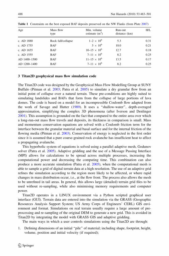
pressures (see Savage 1987; Drake 1990). Similar vertical height loss/run-out ratios of
these flows to normal rock avalanches of similar volumes (Table 1; e.g., Fisher and
Schmincke 1984; Hayashi and Self 1992) is also indicative of granular-like flow processes
with little initial energy input (in contrast with lateral blast-triggered pyroclastic flows).
Observations of the generation of these types of flows (Ui et al. 1999; Nakada and Fujii
1993) show that they typically start by the sudden break-off of large intact portions of hot
lava domes that rapidly disintegrate to generate abundant ash, gas and blocky particles as
they tumble down slope.
Fig. 2 Most recent inundation areas from dome collapse and BAFs, a recently identified ‘‘cold rockcollapse’’ of the remnant dome (Platz 2007), b most recent BAF deposited inundation area (Platz 2007;Cronin et al. 2003)
Nat Hazards (2010) 53:483–501 487
123
3 Titan2D geophysical mass flow simulation code
The Titan2D code was designed by the Geophysical Mass Flow Modelling Group at SUNY
Buffalo (Pitman et al. 2003; Patra et al. 2005) to simulate a dry granular flow from an
initial point of collapse over a natural terrain. These pre-conditions are highly suited to
simulating landslides and BAFs that form from the collapse of large portions of lava
domes. The code is based on a model for an incompressible Coulomb flow adapted from
the work of Savage and Hutter (1989). It uses a ‘‘shallow-water’’, depth-averaged
approximation, simplifying the complex 3D phenomena (after Iverson and Denlinger
2001). This assumption is grounded on the fact that compared to the entire area over which
a long-run-out mass flow travels and deposits, its thickness in comparison is small. Mass
and momentum conservation equations are solved with a Coulomb friction term for the
interface between the granular material and basal surface and for the internal friction of the
flowing media (Pitman et al. 2003). Conservation of energy is neglected in the first order
since it is assumed that a pure coarse-grained rock avalanche has insufficient heat to affect
a propagating avalanche.
This hyperbolic system of equations is solved using a parallel adaptive mesh, Godunov
solver (Patra et al. 2005). Adaptive gridding and the use of a Message Passing Interface
(MPI) allows for calculations to be spread across multiple processes, increasing the
computational power and decreasing the computing time. This combination can also
produce a more accurate simulation (Patra et al. 2005), when the computational mesh is
able to sample a grid of digital terrain data at a high resolution. The use of an adaptive grid
refines the simulation according to the region more likely to be affected, or where rapid
changes in mass distribution occur, i.e., at the flow front. The process also allows the mesh
to be unrefined in tail areas. In general, this allows large (detailed) terrain grid files to be
used without re-sampling, while also minimising memory requirements and computer
power.
Titan2D operates in a LINUX environment via a Python scripted graphical user
interface (GUI). Terrain data are entered into the simulation via the GRASS (Geographic
Resources Analysis Support System; US Army Corps of Engineers’ CERL) GIS envi-
ronment and format. Simulations on real terrain usually require a large amount of pre-
processing and re-sampling of the original DEM to generate a new grid. This is avoided in
Titan2D by integrating the model with GRASS GIS and adaptive gridding.
The main ways in which a user controls simulations using the Titan2D are through:
1. Defining dimensions of an initial ‘‘pile’’ of material; including shape, footprint, height,
volume, position and initial velocity (if required);
Table 1 Constraints on the best exposed BAF deposits preserved on the NW Flanks (from Platz 2007)
Age Mass flowtype
Min. volumeestimate (m3)
Run-outdistance (km)
H/L
c. AD 1880 Rock fall/collapse 1–2 9 106 5.3 0.31
c. AD 1755 BAF 5 9 106 10.0 0.21
c. AD 1655 BAF 10–15 9 106 12.7 0.18
c. AD 1555 BAF 7–11 9 106 8.2 0.25
AD 1400–1500 BAF 11–15 9 106 13.5 0.17
AD 1200–1400 BAF 7–11 9 106 8.2 0.25
488 Nat Hazards (2010) 53:483–501
123

2. A variable that nominally represents the angle of internal friction of the granular pile;
3. A variable that nominally represents the angle of basal friction between the granular
pile and the substrate;
4. A grid by which differing substrates (based on roughness, vegetation, slope) can be
defined, each with differing basal-friction angles (if needed);
5. Stopping criteria to halt the simulation (normally a limit on ‘‘simulated—real time’’ or
the number of computational time steps);
6. Providing a 3D grid containing topographic information (x, y, z; i.e., a Digital
Elevation Model (DEM) for the simulation area).
Outputs of the model (at user-defined time-steps) typically show for each point in
the computational mesh: x-grid coordinate, y-grid coordinate elevation, pile height,
x-momentum, y-momentum.
Titan2D has been applied to and evaluated against small-scale pyroclastic flows, BAFs
and rock avalanches on Volcan de Colima, Mexico (Pitman et al. 2003; Rupp et al. 2006),
El Misti Peru (Delaite et al. 2005) and Little Tahoma Peak (Sheridan et al. 2005). The
outcomes of these studies have highlighted the uncertainties in objectively defining model
input parameters for realistic simulation of local flow conditions. These have hence only
taken a first-order approach to hazard evaluation. For the creation of a hazard map that
encompasses all geologically reasonable possibilities, there is a need to; (1) create a more
encompassing range of probable scenarios for each of these and (2) include a range of
model controlling parameters.
4 Case study—BAF and rock avalanche scenarios at Mt. Taranaki
The last major sequence of dome building, AD 1700–1850, from Mt. Taranaki was fol-
lowed by the westward collapse of around 5 9 106 m3 of rock from the summit area
(Fig. 2), leaving a half-sectioned dome structure at the summit of approximately
2 9 106 m3 (Platz 2007). This collapse is characterised by at least two stages, one
occurring in the late AD 1880s involved pre-cooled dome rock (\Curie Point temperatures
of 350�C) and parts of the underlying hydrothermally altered crater rim. The unit was
confined to within 5.3 km planimetric distance of the summit (Platz 2007). In contrast to
this event, the penultimate eruption episode (Tahurangi episode) dated at AD 1755 was one
of the largest eruptions of the last 800 years. Hot BAF deposits (Tahurangi Breccia, a and
b) extend on the NW sector to between 8 km (b) and [10 km (a) from source (Fig. 2).
The low-energy characteristics of the recent Taranaki BAF and rock avalanche deposits
(Table 1) mean that the Titan2D approach is well suited. In addition, at Mt. Taranaki, a
well constrained fixed point for flow onsets can be assumed, with broad constraints on
potential collapse volumes given from events in the recent past. The limited record of run
out/volumes of past flows is used to determine a first-order estimate of initial volume.
4.1 Digital elevation model
The identification of the source area in the Titan2D computer simulation is one of the key
input parameters, but developing an appropriate DEM provides the basis for any realistic
flow modelling. As with all simulation studies that attempt to use existing depositional
records to evaluate model outputs, the topography representation or DEM used is normally
that of the present day, rather than the ideal of a pre-event terrain model. The only way to
Nat Hazards (2010) 53:483–501 489
123
get around this in normal conditions is to create a detailed geological model of the stra-
tigraphy of mass flow deposits and subtract these thicknesses from the current terrain (e.g.,
Daag 2003) This is made impractical by the fact that BAFs have highly variable deposit
thicknesses within a network of deep, narrow channels and interfluve areas that may
change considerably between events. Despite this, the present topography (as represented
by a 20 m DEM) at Taranaki (over the last 500 years) retains the same overall broad
morphology and channel system down the northwestern slopes into the Hangatahua River
as well as the same type of channel/erosion landforms and vegetation (Lees and Neall
1993) that existed previously. In addition, using a DEM of the current landscape is more
applicable to development of future hazard forecasting and hazard zonation.
The DEM used of Mt. Taranaki was produced from national topographic GIS datasets
(NZMS 260 series, Land Information New Zealand), containing height data as contours
and spot-heights. Using the ArcGIS TOPOGRID (ESRI 2005) command, a DEM was
created with a cell dimension of 20 m. Major drainages and distinctive geomorphic fea-
tures on the volcano are well defined on the DEM, although, in the surrounding ring plain
area with low slopes and few dominant geomorpholoical features, morphological resolu-
tion is lost. The arcgrid DEM was then imported into GRASS GIS as an ascii file and
converted to a GRASS DEM format for use in Titan2D.
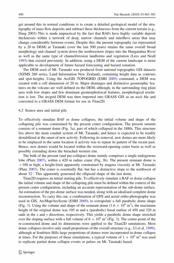
4.2 Source area and initial pile
To effectively simulate BAF or dome collapses, the initial volume and shape of the
collapsing pile was constrained by the present crater configuration. The present summit
consists of a remnant dome (Fig. 3a), part of which collapsed in the 1880s. This structure
lies above the main conduit system of Mt. Taranaki, and hence is expected to be readily
destabilised at the onset of new activity. Following its removal, new domes are more likely
to be emplaced in the same location if activity was to repeat its pattern of the recent past.
Hence, new domes would be located within the westward-opening crater basin as well as
possibly extending down the breached western rim.
The bulk of the present (and pre-collapse) dome mainly comprises a single endogenous
lobe (Platz 2007), within a 420 m radius crater (Fig. 3b). The present remnant dome is
*100 m high, a height-limit apparently constrained by magma viscosity at Mt. Taranaki
(Platz 2007). The crater is essentially flat, but has a distinctive slope to the northwest of
about 328. This apparently generated the ellipsoid shape of the last dome.
Titan2D requires an initial starting pile. To effectively simulate a BAF or dome collapse
the initial volume and shape of the collapsing pile must be defined within the context of the
present crater configuration, including an accurate representation of the sub-dome surface.
An estimation of the pre-dome surface was needed, along with an idealised complete dome
reconstruction. To carry this out, a combination of GPS and aerial ortho-photography was
used in GIS, ArcMap/ArcScene (ESRI 2005), to extrapolate a full parabolic dome shape
(Fig. 3). Using the volume and shape of the remnant dome (1.6 9 106 m3), the maximum
height of the original dome was 105 m and a (parabolic) basal outline of 450 and 320 m
radii in the x and y directions, respectively. This yields a parabolic dome shape stretched
over the sloping surface with a full volume of 6 9 106 m3 (Fig. 3). The centre-point of the
re-constructed dome and its dimensions were applied to the Titan2D simulations. Most
dome collapses involve only small proportions of the overall structure (e.g., Ui et al. 1999),
although at Soufriere Hills large proportions of domes were incorporated in dome collapse
at times. For the purposes of these simulations, a typical volume of 1 9 106 m3 was used
to replicate partial dome collapse events or pulses on Mt. Taranaki based.
490 Nat Hazards (2010) 53:483–501
123

4.3 Titan 2D parameters—basal/internal friction angle
The two ‘‘friction angle’’ parameters used in Titan2D have not been directly related to
physical parameters that can be measured in the laboratory or field. These are normally
calibrated by matching simulation travel times and inundation areas to known values (e.g.,
Schilling 1998; Oramas Dorta et al. 2007). Attempts to determine these parameters
experimentally (e.g., Iverson et al. 1998; Iverson and Denlinger 2001; Bursik et al. 2005)
have focused on the measurement of collapsing piles on tilt tables and on flume experi-
ments. Results are highly variable and it is arguable whether the laboratory conditions can
be scaled to real-world situations. The most commonly used comparator between diverse
types of mass flows is the H/L ratio (Heim friction coefficient; Heim 1932, revised by
Hayashi and Self 1992), which can be used to estimate resistance to flow of a sliding
avalanche by interaction with its underlying surface. Sheridan et al. (2005) used this
method to determine the optimal basal friction parameter for simulating the Tahoma Peak
Avalanche with Titan2D. Sensitivity analysis showed a dramatic effect on increasing
Fig. 3 The dome and reconstruction of initial pile for BAF simulations, a Mt. Taranaki, the current remnantdome, view of the northern side (note person for scale as indicated by the arrow), b ortho-photograph of thesummit and remnant dome, dashed lines indicate the current outline of the remnant dome, solid linesrepresent the reconstructed modelled dome, c GIS representation of dome, 1 Underlying summit surfacewith solid line representing the margins of the remnant dome. 2 3D representation of the current remnantdome, 2 9 106 m3. 3 Reconstructed dome used for BAF simulation 5 9 106 m3
Nat Hazards (2010) 53:483–501 491
123

run-out lengths with reductions in the basal friction angle parameter, whereas changes in
the internal friction angle have shown less dramatic or no noticeable impacts in middle-
value ranges (Sheridan et al. 2005).
For the Mt. Taranaki flows, the only comparative measures available are inundation
area, estimated volume, run-out length and minimum H/L estimates. Rather than choosing
specific values based on this imperfect dataset, a batch of 80 simulations were run for a
controlled initial volume and location with every possible combination of internal and
basal friction angle parameters at intervals of 5�.
4.4 Simulation results
Most simulated BAF deposition surfaces compared well to mapped deposits, without
anomalies, such as overtopping known major topographic barriers or crater walls and
without entering alternative catchments. All simulations exhibited a partial collapse from
the initial pile with flow to the northwest of the current amphitheatre. Within the first
2.5 km from source, simulated flows were confined to a 500 m-wide amphitheatre-like
structure. The flows either stopped on this slope (with high basal friction angles) or
continued into box-shaped gullies of major stream channels (Maero and Pyramid Streams).
After 3.5 km, these tributary flows combined in the Hangahatua (Stony) River valley for a
further 9.5 km of travel.
Each simulation output was processed using GIS to develop an inundation area map of
maximum flow (pile) thickness. With extremely low basal friction angles (58–108) a series
of ‘‘bounce footprints’’ resulted from flows that accelerated unrealistically rapidly down
slope (see Fig. 4). At the opposite end of the spectrum (80–90o basal friction) piles col-
lapsed and halted within \1 km of source. As discovered by Sheridan et al. (2005) vari-
ations in the internal friction angle had very little effect on the final inundation area and
run-out of the flow. This parameter appears to play a more important role on affecting the
velocity outputs of the simulation at particular points in time.
The inundation areas, H/L ratio and run-out planar distance from mapped BAF deposits
and those of simulated BAF’s were most similar with basal friction angles between 15–25�(Fig. 4).
4.5 Deriving hazard representations from the modelled flows
Converting Titan2D simulations of BAFs at Mt. Taranaki to an overall hazard represen-
tation required a method that combined all valid outputs. The approach developed takes
into account variation resulting from the possible range in model input parameters that
were used to infer the variation within realistic geological (or rheological) possibilities for
hot and cold flows and source regions as described earlier.
Using a single volume/source example that is representative of the most recent BAF
events, the model variation is broad with basal friction angles between 158 and 258.A Gaussian distribution was assumed for this range (median = 228) to determine a set of
new basal friction angles (Table 2) that is more representative of the range of possible
events. Using the same initial pile starting conditions, the same DEM, and a fixed internal
friction angle of 308 (based on the previous 80 runs), a series of new simulations was used
to produce a range of outputs that encompass the spectrum of inundation areas and run-outs
expected by BAFs and/or major cold rock avalanches on NW Mt. Taranaki (Fig. 5).
These simulations provide a range of scenario layers that can be further analysed in a
GIS to display estimated flow depths, velocity and discharge. Using ArcGIS (ESRI 2005),
492 Nat Hazards (2010) 53:483–501
123

Do
me0
505
Do
me0
520
Do
me0
535
Do
me1
015
Do
me1
030
Do
me1
510
Do
me1
525
Do
me2
005
Do
me2
020
Do
me2
035
Do
me2
515
Do
me2
530
Do
me2
545
Do
me3
015
Do
me3
030
Do
me3
045
Do
me3
515
Do
me3
530
Do
me3
545
Do
me4
015
Do
me4
030
Do
me4
045
Do
me4
515
Do
me4
530
Do
me4
545
0
4000
8000
12000
16000
20000
24000
Do
me0
505
Do
me0
520
Do
me0
535
Do
me1
015
Do
me1
030
Do
me1
510
Do
me1
525
Do
me2
005
Do
me2
020
Do
me2
035
Do
me2
515
Do
me2
530
Do
me2
545
Do
me3
015
Do
me3
030
Do
me3
045
Do
me3
515
Do
me3
530
Do
me3
545
Do
me4
015
Do
me4
030
Do
me4
045
Do
me4
515
Do
me4
530
Do
me4
545
0
0.2
0.4
0.6
0.8
Do
me0
505
Do
me0
520
Do
me0
535
Do
me1
015
Do
me1
030
Do
me1
510
Do
me1
525
Do
me2
005
Do
me2
020
Do
me2
035
Do
me2
515
Do
me2
530
Do
me2
545
Do
me3
015
Do
me3
030
Do
me3
045
Do
me3
515
Do
me3
530
Do
me3
545
Do
me4
015
Do
me4
030
Do
me4
045
Do
me4
515
Do
me4
530
Do
me4
545
0
20
40
60
80
100
Dis
tan
ce -
Str
aig
ht
Lin
e fr
om
S
ou
rce
(m)
H/L
Rat
io
Are
a O
verl
ap (
%)
Titan2D Runs-Dome(Internal Friction)(Basal Friction)
05 20 30 45
Basal Friction A
B
C
D
Fig. 4 Simulation outputs analysis. Yellow lines highlight best fit. a Summary of initial visual analysis,b comparison of simulations to run-out distance, c comparison of simulations to H/L ratio, d comparison ofsimulations to inundation area
Nat Hazards (2010) 53:483–501 493
123

the outputs of each simulation were processed to produce a point layer containing the
maximum pile height at each processed point. The point dataset was interpolated to create
a raster grid of pile-heights across the region. This produces a laterally and longitudinally
gradational continuous layer. Raster layers from each of the simulations were combined
into a single height/thickness layer using the ArcGIS raster calculator tool. This combined
‘‘thickness’’ layer was chosen to be directly represented as a gradational hazard zone
(Fig. 5). A similar process can also be paralleled for velocity or momentum outputs
depending on user engineering or human hazard needs.
This combined layer highlights the Stony River and catchments as areas of greatest
hazard as expected. It can be queried at user-defined points and displayed using a variety of
underlying images, maps or infrastructure networks, as well as displayed in 3D with a
shaded-relief model or ortho-image draped over a DEM (Fig. 5).
5 Discussion
5.1 Combined simulated results
The results and a 1:300 year (based on Neall and Alloway 1996, return period for hazard
zone A) hazard zone from BAFs are defined by the area (darker red central hazard zone on
Fig. 5) associated with the drainage patterns of the northwestern sector of the volcano.
These areas have been inundated by all BAFs in the past c. 800 years (Platz 2007). The
gradational zone, however, shows a lessening decrease in hazard on the interfluves between
the main drainages, indicating the lower possibility of flows inundating these (Fig. 5). Of
particular interest is the length of the hazard zone highlighting that flows would only rarely
reach lower altitudes (700 m, [10 km run-out), which is consistent with field evidence
(Platz 1997).
5.2 Mass flow hazard simulation
The majority of volcanic flow hazard maps are generalisations based solely on extrapo-
lating the past inundation areas of each type of flow (e.g., pyroclastic flow, lahar, debris
avalanche) onto present topography (Scott et al. 1995; Waitt et al. 1995; Hoblitt et al. 1998;
Table 2 Basal friction anglesused in the Titan2D simulationsfor the hazard zone model forBAFs at Mt. Taranki
Run Basal friction Gausian distribution (%)
1 17.6305 0.0333
2 18.1747 0.0747
3 19.103 0.1095
4 20.333 0.1346
5 21.7556 0.1478
6 23.2444 0.1478
7 24.667 0.1346
8 25.897 0.1095
9 26.8253 0.0747
10 27.3695 0.0333
494 Nat Hazards (2010) 53:483–501
123

Wolfe and Pierson 1995). These become redundant when either new mapping identifies
additional constraints on event frequency or inundation or when eruptions/collapses sub-
stantially change the topography. In addition, hazard maps for land-use planning, work-
place and recreational area management require more precision to reliably indicate
differing degrees of relative hazard. In addition, other information, such as flow velocity,
depth and mass flux is essential for assessing the stability of any structures in the flow path
and planning any new infrastructure. However, hazard maps showing increasingly more
complexity, including those with some probabilistic component (e.g., Nevado del Ruiz;
Parra and Cepeda 1990) are typically less well understood by users.
For current tephra fall hazards, Magill et al. (2006) used the numerical model ASH-
FALL (Hurst 1994) to forecast the probability of volcanic ashfalls from all major sources
to affect the city of Auckland. From these data, they determined and displayed tephra
inundation maps of a similar nature to those presented here. Using an alternative approach,
Bebbington and Lai (1996) and Turner et al. (2008) developed a time-variable, probabil-
isitic, ashfall forecast for Taranaki. These statistical approaches may be divorced by
varying degrees from the physical hazard generation processes, particularly those that
combine various physical models without considering their inherent uncertainties. Other
limiting factors with these methods are the ability to produce spatial representations
Fig. 5 a Hazard zone created from Titan2D computer simulations based on the a 1:300 year BAF eventfrom a dome collapse and b 3D representation of the created Hazard zone
Nat Hazards (2010) 53:483–501 495
123

(i.e., hazard maps) of the predictions that can be easily understood and applied by local
authorities, land-use planners and hazard/emergency managers.
A similar approach to the Taranaki example presented here was undertaken for mass
flows landslide and rock/debris flow hazards in the District of North Vancouver (Jacob
2005; KWL Ltd. 2003) using Flo-2D software (FLO-2D Software Inc.) to recreate the
discharge/inundation of flows of a particular recurrence period. Inundation maps of each
simulated flow in the various catchments studied were combined in a GIS to give a
representation of the hazard to downstream areas. A gradation of increasing relative hazard
was defined on the basis of the likelihood of areas being affected. The range of volumes
modelled also provides a good method for encompassing and compensating for the lack of
uncertainty around the volume of future events. This method does not, however, take into
account the variability in the physical properties of the flow and whether these can be
accounted for by the model. The recognition of the variability that may exist due to
changing or contrasting flow sediment concentrations and differing flow paths was entirely
assumed to be a factor of volume. The methods presented for the Taranaki example differ
by attempting to identify a range within the input (physical) parameters that influence the
flow rheology (largely unknown here) and resulting inundation area. This is then used as a
proxy to encompass all the realistic possible outcomes within the constraints of recent past
events. As identified by Platz et al. (2007), we can identify or infer from deposits that flows
and their behaviour (linked to emplacement processes) can vary greatly and this can have
an effect on run-out and inundation. It is assumed that in the Titan2D model friction input
values are the most influential parameters in the flow model that control the modelled flows
mobility. For the Mt. Taranaki BAFs, the rheology of the flow (rather than source con-
ditions) is one of the more dominant factors in determining the run-out and inundation.
To expand this by including the variability amongst all known or possible BAFs on
Taranaki events (such as variations in initial volume and source) would require either
having a complete event history with accurately known volumes and inundation areas, or
developing a probabilistic model to describe the known limits of variation in these that
could then be coupled to Titan2D.
Given the relative dominance of BAF and related mass flows over the last 800 years, the
simulations made are more likely to encompass the main initial hazards of the next unrest
at Mt. Taranaki. The present configuration means that collapses down the NW slope will be
highly likely if a new dome were to grow. The maximum volume that could be accom-
modated in the present crater is around *10 9 106 m3, similar to the total volume of the
largest sets of flow-packages mapped to date. It is common that only small fractions of
dome volumes collapse at any one time (Unzen Volcano (eruption c. 1991), Nakada and
Fujii 1993; Gunung Merapi Volcano (eruption c. 1993), Schwarzkopf et al. 2005), which
further reduces the probable volumetric range of flows expected.
5.3 Taranaki BAF hazard mapping
Grant-Taylor (1964) and Neall (1972) considered that potential risk from future pyroclastic
flow (BAF) activity at Mt. Taranaki would be restricted to within a 9 km radius of the
summit. This was followed by a hazard map for volcanic flows (Neall and Alloway 1996)
that defined six zones of risk, from various types of mass flows. This was based on mapped
historical and prehistoric deposits of pyroclastic flows, lahars and debris avalanches along
with their estimated return periods. The two zones relating to pyroclastic flows are defined
by a radius of 15 km from the summit, with the highest hazard zone having a 1 in 300 year
return period of impact. Recent studies (Turner et al. 2008; Platz 2007) have revealed a
496 Nat Hazards (2010) 53:483–501
123

much higher frequency of small-volume dome collapse and pyroclastic-flow producing
eruptions, necessitating a revision of the hazard zones. In addition, questions remain as to
how accurate the map remains in the context of present-day topography, particularly in
relation to a future ‘‘typical’’ sequence of dome growth and collapse with a crater area open
and sloping towards the NW.
The 15 km-circular hazard zone of Neall and Alloway (1996) incorporates the extent of
all possible pyroclastic flows that may originate from the volcano. This may be a useful
overall ‘‘exclusion zone’’ for emergency management during a volcanic crisis due to the
unpredictable nature and path of pyroclastic flows, associated surges, ballistics, tephra and
possible blast events. However, this approach does not allow distinction of varying degrees
of mass flow risk in the area for the managers of recreational area (and workplace) between
eruptions and even during prolonged eruptions. Nor does it allow identification of any key
infrastructure elements that may be affected with greatest likelihood by mass flows, such as
critical bridges, pipe lines and power cables. Given that BAFs and other mass flows since
ca. 800 years have almost exclusively affected the NW sector, this is the area of highest
apparent risk under present topographical conditions yet this is not represented in hazard
zones due to larger events (with less probability of occurrence) overshadowing this area of
higher risk. However, it must be recalled that the newly created hazard zone is scenario-
based rather than encompassing all of these events possibly originating from the summit
and considered by Neall and Alloway (1996) to have a return period of 1:300 years based
on the last 1,000 years of events.
There are few examples of applying a numerical model or computer simulation to
hazard analysis and determination of future high risk zones other than that of Saucedo et al.
(2005). The majority of computer model applications are related to the comparison of real
and modelled simulations or the optimisation of parameters within a model. The method
presented here explores this premise in relation to a scenario in which BAFs from the same
part of the volcano or sequence of dome collapses may vary greatly. It is apparent that for
the Titan2D model, friction input values are the most influential parameters, which appears
also to be the case for the Mt. Taranaki examples, where source differences matter less.
By varying these factors we can account for expected variance in future Mt. Taranaki
BAFs, during the course of a dome growth and collapse sequence. By modelling a range
around an optimally compared flow, we can account for the variation that might exist by
combining and displaying all results. The Gaussian distribution was used to encompass the
variability observed in inundation areas. These give rise to GIS layers that can be displayed
to show the gradational nature of hazard assessment, as implied by the early workers
quoted earlier in this article.
Haynes et al. (2007) provided important observations about the effectiveness of tradi-
tional hazard maps in relation to public interpretations of them. They found that respon-
dents could better orientate themselves and interpret hazard zone information in 3D format
or data that was superimposed onto photographs or aerial photographs. Titan2D outputs
and use of a GIS easily enable overlays of hazard zones onto aerial/satellite imagery or
shaded-relief models to facilitate this knowledge transfer (Fig. 5).
6 Conclusions
Titan2D provides a tool that can simulate granular flows and provide outputs that are
testable within geological mapping constraints. Multiple runs can be undertaken rapidly on
a desktop computer and allow for timely hazard assessments to be made on present-day
Nat Hazards (2010) 53:483–501 497
123

terrain, or on terrain that is rapidly changing. This case study shows that by undertaking an
initial series of Titan2D runs that incorporate all reasonable combinations of basal and
internal friction angles for BAFs while keeping the source conditions constant, best-fit
simulations can be determined by comparison to the spatial distribution of known BAF
events (Platz 2007). Here, reasonable Titan2D input parameters were 15–208 for basal
friction and 308 for internal friction. Using this, a Gaussian distribution of new input
parameters could be derived to produce a series of new titan simulations. The combination
of the inundation areas from these new simulations allowed for the creation of a graduated
zone of inundation likelihood. This method provides a means to account for uncertainty
related to differences in flow behaviour of BAFs or similar granular flows. The digital
outputs from Titan2D can be displayed in GIS and presented with aerial, satellite imagery
or in 3D to allow the user a greater understanding of the relationship between the possible
hazard and the landscape.
Iverson (2005) remarks that ample scepticism should be used when scientific inter-
pretations are made from models and all physical, mathematical and computational aspects
need to be understood. This is applicable for hazard analysis also, particularly when
volcanic flow hazard analysis methods and the display of hazard zones have developed
little since Crandell et al. (1984). Flow modelling is becoming a more common practise in
volcanic hazard analysis, but mostly in relation to single events or scenarios. Despite the
rapid use and uptake of the results produced from computer simulations of flows (par-
ticularly by local government/authority in land use planning), there has been very little
effort to transfer that information into publicly available hazard maps. This comes, how-
ever, with the danger that appropriate representation of inherent uncertainties may be
overlooked. Even in traditional hazard analysis and mapping based on geological field
identification, uncertainty exists in both the inundation area and volume of a particular
deposit as well as in the stratigraphic interpretation of the return period. However, these
uncertainties are rarely transferred onto the cartographic display of the hazard. The
identification and quantification of uncertainty and display of model simulations related to
hazard analysis is an area that requires more attention to provide both the geologist and the
user with a simple display of the potential risk.
Acknowledgments This work is supported by a NZ FRST TPMF PhD fellowship (JP), and forms part ofthe FRST PGST programme contract MAUX0401 ‘‘Learning to live with volcanic risk’’ (SJC). We alsothank the George Mason Trust and Freemasons for scholarship support and Dr. R.B. Stewart for commentson an earlier version. We also thank Prof. J-C. Thouret and Prof. C. Siebe for their thoughtful reviewcomments and assistance.
References
Alloway B, McComb P, Neall V, Vucetich C, Gibb J, Sherburn S, Stirling M (2005) Stratigraphy, age, andcorrelation of voluminous debris avalanche events from an ancestral Egmont Volcano: implications forcoastal plain construction and regional hazard assessment. J R Soc NZ 35:229–267
Bebbington MS, Lai CD (1996) Statistical analysis of New Zealand volcanic occurrence data. J VolcanolGeoth Res 74:101–110
Bonadonna C, Connor CB, Houghton BF, Connor LJ, Byrne M, Laing A, Hincks TK (2005) Probabilisticmodeling of tephra dispersal: hazard assessment of a multiphase rhyolitic eruption at Tarawera, NewZealand. J Geophys Res 110:B03203. doi:10.1029/2003JB002896
Boudon G, Camus G, Gourgand A, Lajoie J (1993) The 1984 nuee ardente deposits of Merapi volcano,Central Java, Indonesia: stratigraphy, textural characteristics, and transport mechanisms. Bull Volcanol55:327–342
498 Nat Hazards (2010) 53:483–501
123

Bursik M, Patra A, Pitman EB, Nichita C, Macias JL, Saucedo R, Girina O (2005) Advances in studies ofdense volcanic granular flows. Rep Prog Phys 68:271–301. doi:10.1088/0034-4885/68/2/R01
Canuti P, Casagli N, Catani F, Falorni G (2002) Modeling of the Guagua Pichincha volcano (Ecuador)lahars. Phys Chem Earth Parts A/B/C 27(36):1587
Cole PD, Calder ES, Sparks RJS, Clarke A, Druitt TH, Young SR, Herd RA, Harford CL, Norton GE (2002)Deposits from dome collapse and fountain collapse pyroclastic flows at Soufriere Hills Volcano,Montserrat. In: Druitt TH, Kokelaar BP (eds) The Eruption of Soufriere Hills Volcano, Montserrat,from 1995 to 1999. Memoirs, vol 21. Geological Society, London, pp 231–262
Crandell DR, Booth B, Kazumadinata K, Shimozuru D, Walker GPL, Westercamp D (1984) Source bookfor volcanic hazards zonation. UNESCO, Paris
Cronin SJ, Stewart RB, Neall VE, Platz T, Gaylord D (2003) The AD1040 to present Maero Eruptive Periodof Egmont Volcano, Taranaki, New Zealand. Geol Soc NZ Misc Publ 116A:43
Delaite G, Thouret J-C, Sheridan M, Labazuy P, Stinton A, Souriot T, Van Westen C (2005) Assessment ofvolcanic hazards of El Misti and in the city of Arequipa, Peru, based on GIS and simulations, withemphasis on lahars. Zeitschrift fur Geomorphol NF 140:209–231
Drake TG (1990) Structural features in granular flows. J Geophys Res 95(B6):8681–8696ESRI ArcGIS (2005) Environmental systems research Inc. USAFisher RV, Schmincke H-U (1984) Pyroclastic rocks. Springer, Berlin, p 472Grant-Taylor TL (1964) Geology of Egmont National Park. In: Scanlan AB (ed) Egmont National Park.
Egmont National Park Board, New Plymouth, pp 13–26Hayashi JN, Self S (1992) A comparison of pyroclastic flow and debris avalanche mobility. J Geophys Res
97:9063–9071Haynes K, Barclay J, Pidgeon N (2007) Volcanic hazard communication using maps: an evaluation of their
effectiveness. Bull Volcanol 70(2):123–138Heim A (1932) Der Bergstruz von Elm. Geol Gesell Zeitschr 34:74–115Hoblitt RP, Walder JS, Driedger CL, Scott KM, Pringle PT, Vallance JW (1998) Volcano hazards from
Mount Rainier, Washington, Revised 1998: US Geo Surv Open-File Report, 98–428Hurst AW (1994) ASHFALL—a computer program for estimating volcanic ash fallout. Report and users
guide. Institute of Geological & Nuclear Sciences Science Report 94/23. 22Itoh H, Takahama J, Takahashi M, Miyamoto K (2000) Hazard estimation of the possible pyroclastic flow
disasters using numerical simulation related to the 1994 activity at Merapi Volcano. J VolcanolGeotherm Res 100(1–4):503–516
Iverson R (2005) Debris-flow mechanics. In: Jakob M, Hungr O (eds) Debris-flow hazards and relatedphenomena. Praxis-Springer, Heidelberg, pp 105–134
Iverson RM, Denlinger RP (2001) Flow of variably fluidized granular material across three dimensionalterrain 1: Coulomb mixture theory. J Geophys Res 106:537–552
Iverson RM, Schilling SP, Vallance JW (1998) Objective delineation of lahar-inundation hazard zones. GeolSoc Am Bull 110:972–984
Jacob M (2005) Debris-flow hazards analysis. In: Jakob M, Hungr O (eds) Debris-flow hazards and relatedphenomena. Praxis-Springer, Heidelberg, pp 411–443
KWL Ltd (2003) Debris flow study and risk mitigation alternatives for Percy Creek and Vapour Creek.(Final Report, December). District of North Vancouver
Lees CM, Neall VE (1993) Vegetation response to volcanic eruptions on Egmont volcano, New Zealand,during the last 1500 years. J R Soc NZ 23:91–127
Magill C, Hurst A, Hunter L, Blong R (2006) Probabilistic tephra fall simulation for the Auckland Region,New Zealand. J Volcanol Geotherm Res 153(3–4):370–386
Malin MC, Sheridan MF (1982) Computer-assisted mapping of pyroclastic surges. Science 217:637–640Miyabuchi Y (1999) Deposits associated with the 1990–1995 eruption of Unzen volcano, Japan. J Volcanol
Geotherm Res 89:139–158Nakada S, Fujii T (1993) Preliminary report on the activity at Unzen Volcano (Japan), November 1990–
November 1991: Dacite lava domes and pyroclastic flows. J Volcanol Geoth Res 54(3–4):319–333Neall VE (1972) Tephrochronology and tephrostratigraphy of western Taranaki, New Zealand. NZ J Geol
Geophys 15:507–557Neall VE (1979) Sheets P19, P20 and P2 l New Plymouth, Egmont and Manaia, Geological Map of New
Zealand. New Zealand Department of Science and Industrial Research, Wellington, scale 1:50 000, 3sheets, 36pp
Neall VE, Alloway BE (1996) Volcanic hazard map of Western Taranaki. Massey Uni Dep Soil Sci OccReport 12
Nat Hazards (2010) 53:483–501 499
123

Oramas Dorta D, Toyos G, Oppenheimer C, Pareschi MT, Sulpizio R, Zanchetta G (2007) Empiricalmodelling of the May 1998 small debris flows in Sarno (Italy) using LAHARZ. Nat Hazards 40:381–396
Palladino DM, Valentine GA (1995) Coarse-tail vertical and lateral grading in pyroclastic flow deposits ofthe Latera Volcanic Complex (Vulsini, Central Italy): origin and implications for flow dynamics.J Volcanol Geotherm Res 69:343–364
Parra E, Cepeda H (1990) Volcanic hazard maps of the Nevado del Ruiz Volcano, Colombia. J VolcanolGeotherm Res 42:117–127
Patra AK, Bauer AC, Nichita CC, EPitman EB, Sheridan MF, Bursik M, Rupp B, Webber A, Stinton AJ,Namikawa LM, Renschler CS (2005) Parallel adaptive numerical simulation of dry avalanches overnatural terrain. J Volcanol Geotherm Res 139(1–2):89–102
Pitman EB, Nichita CC, Patra A, Bauer A, Sheridan MF, Bursik MI (2003) Computing granular avalanchesand landslides. Phys Fluids 15(12):3638–3646
Platz T (2007) Aspects of dome-forming eruptions from Andesitic Volcanoes exemplified through theMaero Eruptive Period (1000 yrs B.P. to Present) activity at Mt. Taranaki, New Zealand. UnpublishedPhD thesis, Institute of Natural Resources, Massey University, Palmerston North, New Zealand
Platz T, Cronin SJ, Cashman KV, Stewart RB, Smith IEM (2007) Transitions from effusive to explosivephases in andesite eruptions—a case-study from the AD1655 eruption of Mt. Taranaki, New Zealand.J Volcanol Geotherm Res 161:15–34
Rupp B, Bursik M, Patra A, Pitman B, Bauer A, Nichita C, Saucedo R, Macias J (2003) Simulation ofpyroclastic flows of Colima volcano, Mexico, using the TITAN2D program, AGU/EGS/EUG Spg.Meet. Geophys Res Abstracts 5:12857
Rupp B, Bursik M, Namikawa L, Webb A, Patra AK, Saucedo R, Marcias JL, Renschler C (2006) Com-putational modelling of the 1991 block-and-ash flows at Colima Volcano, Mexico. In: Seibe C,Marcias JL, Aguirre-Diaz GJ (eds) Neogene-Quaternary Continental Margin Volcanism: a perspectivefrom Mexico. Geol Soc Am Spec Paper, 402:237–250
Saucedo R, Macıas JL, Bursik MI (2004) Pyroclastic flow deposits of the 1991 eruption of Volcan deColima, Mexico. Bull Volcanol 66:291–306
Saucedo R, Macias JL, Sheridan MF, Bursik MI, Komorowski JC (2005) Modelling of pyroclastic flows ofColima Volcano, Mexico: application to hazard assessment. J Volcanol Geotherm Res 139(1):103–115
Savage SB (1987) Interparticle percolation and segregation in granular materials: a review. In: SelvaduraiAPS (ed) Developments in engineering mechanics. Elsevier, New York, pp 347–363
Savage SB, Hutter K (1989) The motion of a finite mass of granular material down a rough incline. J FluidMech 199:177–215
Schilling SP (1998) LAHARZ: GIS programs for automated mapping of Lahar-inundation hazard zones. USGeo Surv Open-File Report 98–63
Schwarzkopf LM, Schmincke H-U, Cronin SJ (2005) A conceptual model for block-and-ash flow basalavalanche transport and deposition, based on deposit architecture of 1998 and 1994 Merapi flows.J Volcanol Geotherm Res 139:117–134
Scott WE, Iverson RM, Vallance JW, Hildreth W (1995) Volcano hazards in the Mount Adams Region,Washington: US Geo Surv Open-File Report 95–492, 11pp
Scott KM, Macıas JL, Naranjo J, Rodriguez S, McGeehin JP (2001) Catastrophic debris flows transformedfrom landslides in volcanic terrains: mobility, hazard assessment and mitigation strategies. US GeolSurv Prof Pap 1630:59
Sheridan MF, Hubbard B, Carrasco-Nunez G, Siebe C (2000) GIS model for volcanic hazard assessment:pyroclastic flows at Volcan Citlaltepetl, Mexico. In: Parks BO, Clarke KM, Crane MP (eds) Pro-ceedings of the 4th international conference on integrating geographic information systems andenvironmental modeling: problems, prospects, and needs for research; 2000 September 2–8; Boulder,CO. Boulder: University of Colorado, Cooperative Institute for Research in Environmental Science
Sheridan MF, Stinton AJ, Patra AK, Bauer AC, Nichita CC, Pitman EB (2005) Evaluating TITAN2D mass-flow model using the 1963 Little Tahoma Peak avalanches, Mount Rainier, Washington. J VolcanolGeotherm Res 139(1–2):89–102
Sparks RSJ, Young SR (2002) The eruption of Soufriere Hills Volcano, Montserrat (1995–1999). In: DruittTH, Kokelaar BP (eds) The Eruption of Soufriere Hills Volcano, Montserrat, from 1995 to 1999, GeolSoc London Memoirs 21:45–69
Stevens NF, Manville V, Heron DW (2003) The sensitivity of a volcanic flow model to digital elevationmodel accuracy: experiments with digitised map contours and interferometric SAR at Ruapehu andTaranaki volcanoes, New Zealand. J Volcanol Geotherm Res 119:89–105
Toyos G, Cole P, Felpeto A, Martı J (2007) A GIS-based methodology for hazard mapping of small volumepyroclastic flows. Nat Hazards 41:99–112
500 Nat Hazards (2010) 53:483–501
123

Turner MB, Cronin SJ, Bebbington MS, Platz T (2008) Developing a probabilistic eruption forecast fordormant volcanoes; a case study from Mt. Taranaki, New Zealand. Bull Volcanol 70:507–515. doi:10.1007/s00445-007-0151-4
Ui T, Matsuwo N, Sumita M, Fujinawa A (1999) Generation of block and ash flows during the 1990–1995eruption of Unzen volcano, Japan. J Volcanol Geotherm Res 89:123–137
Waitt RB, Mastin LG, Beget JE (1995) Volcanic-hazard zonation for Glacier Peak Volcano, Washington.US Geo Surv Open-File Report 9:5–499
Wolfe EW, Pierson TC (1995) Volcanic-Hazard Zonation for Mount St. Helens, Washington, 1995. US GeoSurv Open-File Report 9:5–497
Zernack A, Procter J, Cronin SJ (2009) Sedimentary signatures of cyclic growth and destruction ofstratovolcanoes: a case study from Mt. Taranaki, New Zealand. In: Nemeth K, Manville V, Kano K(eds) Source to sink: from volcanic eruptions to volcaniclastic deposits on the Pacific Rim. IUGS,Special Volume Sedimentary Geology (in press)
Nat Hazards (2010) 53:483–501 501
123
Copyright © 2022 FDOKUMEN

