


Bahasa
Halaman
Hukum


1
Published in: Archaeology at the Interface. Edited by G. Burenhult and J. Arvidssen. ArcheoPress (Brisitish Archaeological Reports
International series). Oxford, 2002.
TTHHEE SSTTAATTIISSTTIICCSS OOFF AARRCCHHAAEEOOLLOOGGIICCAALL
DDEEFFOORRMMAATTIIOONN PPRROOCCEESSSSEESS..
AAnn aarrcchhaaeeoozzoooollooggiiccaall eexxppeerriimmeenntt
Laura MAMELI,
Juan A. BARCELO ,
Jordi ESTEVEZ,
Divisió de Prehistòria
Facultat de Lletres. Edifici B
Universitat Autònoma de Barcelona
E-08193 Bellaterra Spain
[email protected] [email protected] [email protected]
ABSTRACT
The quantification of faunal bone assemblages from archaeological sites has a long tradition. Nevertheless, in
most cases those studies are somewhat “passive”, as if the bones have always been in those conditions,
waiting for the archaeologist. There are many taphonomic studies to solve these problems, but in most
occasions, taphonomic results seem totally unrelated to archaeological research, as if the natural factors were
studied independently from social factors.
In this paper we present a case study where the natural formation process of bone assemblages is
experimented. Contrary to the usual view, when wild animals (scavengers) are the causal agent of the
assemblage, the archaeologically observable consequence is not an accumulation of bones, but a considerable
spread of them. As a result, bones enter into the archaeological record as individual items, without an
understandable spatial pattern.
We have studied 30 animal carcases scavenged by foxes in Tierra del Fuego (Argentina). A general statistical
analysis of those examples is presented in order to describe an important “archaeological de-formation
process”. The goal of the study is to discuss how to analyse de-formation process of the archaeological record,
and how they affect the quantification of faunal remains in archaeological sites.
KEY WORDS: Zooarchaeology, Spatial Archaeology, Formation Process, Correspondence
Analysis, Disturbance, Post-Depositional alteration

2

3
1. THE DEFORMATION OF ARCHAEOZOOLOGICAL ASSEMBLAGES
Archaeologists traditionally have drawn their inferences about past behaviour from dense, spatially discrete
aggregations of artefacts, bones, features, and debris. They have traditionally assumed that the main agent
responsible for creating such aggregates was only human behaviour. Even though nowadays most
archaeologists are aware of natural disturbance process and the complexities of archaeological formation,
archaeological contexts are still usually viewed as a deposit or aggregate of items, which are part of single
depositional events. We usually speak of human behaviour being fossilised in archaeological accumulations
or deposits, as if the materials of social action through time were only accumulative.
In the case of faunal processing, the “supposed” main observable consequences of social action are bone
accumulations. The underlying idea seems to be that the bones of the creatures under consideration have
survived since deposition to a more-or-less similar extent, and that the relative abundance of species is
representative of that originally deposited. However, the accumulation of animal bones in the archaeological
record not always is the result of purposeful human activity. An aggregation of bones may not reflect past
human social action, but rather post depositional processes. Loss, discard, reuse, decay, and archaeological
recovery are numbered among the diverse formation processes that in a sense, mediate between the past
behaviours of interest and their surviving traces (see among others Meadow 1976, Hassan 11998877,, Schiffer
1987). Most post-depositional processes make archaeozoological assemblages more amorphous, lower in
elements density, more homogeneous in their internal density, less distinct in their boundaries, and more
similar (or at least skewed) in composition. Those processes have the effect of disordering artefact patterning
in the archaeological record, and increasing entropy. Furthermore, some post-depositional disturbance
process may increase the degree of patterning of artefact disturbances, but towards natural arrangements
(Ascher 1968, Carr 1984). Consequently, determining whether the various frequencies of items in an
assemblage or deposit have resulted from undisturbed deposition, differential distribution, differential
preservation is the problem (Brain 1980, Lyman 1987).
Archaeological assemblages should be regarded as aggregates of individual elements, which interact with
various agents of modification in statistical fashion, with considerable potential for variation in the traces they
ultimately may show. Cowgill (1970) proposed a preliminary solution: we have to recognize three basic
populations (in the statistical sense):
(1) events in the past,
(2) material consequences created and deposited by those events, and
(3) artefacts that remain and are found by the archaeologist (“physical finds”).
By stressing the discontinuities, Cowgill states for viewing formation process as agents of bias within a
sampling framework. At the beginning, material items are organized in the archaeological record in a way
coherent with the resource management strategies and social practices that generated them. Once the location
of social action was left, those remains were subject to bio-geologic forces, which introduce a new material
organization. This new patterning of social material remains is opposite to the original pattern, and
consequently increases entropy (des-organization, chaos, and ambiguity), until the original patterning become
unrecognisable. Each population is then a potentially biased sample drawn from the previous population that
was itself a potentially biased sample. We may view these discontinuities as sampling biases in the sense that
what we recover and observe does not proportionately represent each aspect of the antecedent behaviour.
From our dialectic point of view, changes and transformations in the original patterning of activity sets are not
a simple accumulation process from low entropy sets (primary deposition) to higher entropy patterns
(disturbed deposits), but a non-linear sum of quantitative changes, which beyond a threshold, produce a
qualitative transformation. A depositional set may be thought of as a mathematical set, the organization of
which is the end product of structural transformations operating upon a previously structured set. In this
sense, the occurrence of specific formation process is determined by specific causative variables. That means,
that depending of the degree of entropy, the transformed archaeological set is not necessary a random sample
of the original population. That is, the difference between a depositional and an activity set is based on a
deep qualitative discontinuity generated by the aggregate of minor quantitative modifications (Estevez 2000).
The main point is not the recovery of the “social action direct effect” by reversing the formation process of
“depositional sets” (for definitions, see Carr 1984, Urbancyk 1986). Rather, the processes responsible for
generating organizing, preserving, and presenting the archaeological record should be viewed simply as a
dialectic formation processes. Attention should be drawn to the dynamic life history of archaeological remains

4
and the processes of different temporal frequency on the ultimate position, content, and pattern of
archaeological remains. This perspective provides a strong antidote to the facile “reconstruction of culture” by
“correcting” for apparent disturbances or distortions.
2. SUBSTRACTION AS AN ARCHAEOLOGICAL FORMATION PROCESS
In most archaeological bone assemblages, for any given species the frequencies of different skeletal elements
show at least some significant departures from the frequencies in which they would be represented in
complete skeletons. Modifications in original skeletal frequencies may appear: as a result of human actions,
as a result of subtraction by animal scavenging, or as a result of differential preservation and recovery (Klein
1980, Monahan 1998, Bartram & Marean 1999, Estevez 2000).
There is a long discussion whether the difference between primary deposition of animal bones and the
recovered bones may bear directly on the distinction of hunting from scavenging at archaeological sites. Since
the days of Efremov (1940), archaeologists are looking for regular relevant linkages –signature criteria-
between static attributes of the archaeological record and their dynamic causes and associations. A signature
criterion is a criterion that is constant and unique and that discriminates one modifying agent or set of agents
from another. The idea of some authors is to create a dictionary of material consequences of human hunting
and animal scavenging to be able to “predict” the structure of the assemblages produced by a specific action.
These predictions should be tested experimentally, that is, by evaluating the predictions in light of modern
assemblages known to have been formed by the process stipulated in the predictions (Gifford 1981, Binford
1981, Schiffer 1987, Dominguez-Rodrigo 1999). For instance, scavenged assemblages appear to be without
some bones selected by size, weight and shape according to the particular size, mechanical capacity, and
foraging range of the scavenger. Recognizable signatures therefore can be characterized by specific ranges of
taphonomic loose, generally defined through upper size and weight limits (Marean & Bertino 1994,
Stahl1996). For instance, an over-abundance of cranial and distal limb elements of middle-to-big sized game
would be characteristic of butchery sites, whereas the over-abundance of proximal limbs would be a
definitional feature of consumption sites (Binford 1981, Stahl 1999). That means that a characteristic
“human” pattern of disarticulation would be the refuse of lower legs because they lack sufficient meat to
make them desirable. The heavier and less nutritious portions of a carcass (the axial skeleton) tend to remain
at animal death sites, while the lighter and more nutritious portions of a carcass (the appendicular skeleton or
limbs) tend to be transported more extensively away from animal death sites.
But nothing is so easy. The actual combination of those variables related to causal processes that could have
given rise to specific deposits is nearly infinite, and so one cannot expect to find many simple
correspondences between a priori lists of evidences and the characteristics of specific deposits. Bone
subtraction also appears under the form of differential preservation. Under a given destructive regime, the
individual parts will survive in proportion to their robusticity. Survival may be correlated with the
compactness of the bone, expressed as specific gravity (Brain 1980). Skeletal parts of high utility tend to be
low in density, and then those bones are not resistant to damage (Lyman 1987, Rogers 2000): an assemblage
dominated by parts of low utility is also likely to be dominated by parts that are dense and therefore resistant
to scavenger gnawing. Such an assemblage could have been produced either by selective transport or by
selective destruction of low-density parts
One can hardly argue that uniformitarian principles may be formulated concerning the social scope of human
communities, given the profoundly varied, and specific exploitation strategies of resources by different
societies (Hassan 1987, Castro et al. 1993, Marciniak 1999). There are many actions and processes, both
social and natural having acted during and after a primary cause, and also primary causes act with different
intensities and in different contexts, in such a way that effects may seem unrelated with causes.
The fact that we cannot predict the degree a bone assemblage has been scavenged, does not mean we cannot
analyse an animal carcass as a by-product of a series of social actions and which has been altered by other
processes (or the reproduction of the same actions at the same place). In most real cases, we should speak
about multiple causes and complex causal relationships, rather than indeterminism or intrinsic randomness. In
this paper we are interested in measuring the probability an archaeological assemblage of animal bones can be
“deformed” by the action of scavenging. We think that the aggregate of quantitative modifications
experimented by a carcass (in content and spatial distribution) can produce a significative qualitative change
(a bone assemblage). Scavenging should be considered as a sequence of modifications which convert an
animal carcass into a disintegrated set of bones. It is no more an animal, but it contains some distorted
elements of what once was (palimpsest). Given the probabilistic nature of causal relationships, we cannot
assert that, the survival parts of a skeleton will follow an entirely predictable pattern if the destructive

5
influences are known (Brain 1980, p. 117). That means, that simple documentation of frequencies of
disarticulated and articulated joints in an assemblage may not permit the inferential identification of social
action before/after/in absence of subtraction by scavenging.
We have designed a series of controlled observations in order to be able to calculate the probability
relationship between the disturbance effect and the composition and spatial pattern of bone remains. That is,
causal significance of scavenger activity for bone assemblages composition and spatial patterning corresponds
to the difference that the presence or absence of scavenger activity makes on the features of bone
assemblages. In terms of Stochastic Interaction, the probability of existence for scavenger activity and the
features of bone assemblages are determined reciprocally. Therefore, changes in the probability of scavenger
disturbance determine changes in the probability of spatial patterning of bones and changes in the probability
of spatial patterning determine changes in the probability of scavenger activity. We want to test the
hypothesis that an increasing skeletal disorganization in terms of taphonomic loose suggests a more complex
archaeological formation history.
3. TIERRA DEL FUEGO. AN ARCHAEOZOOLOGICAL CASE STUDY
We have studied 30 carcases of “guanaco” (Lama guanicoe, a comparable middle sized herbivore) scavenged
by foxes in Tierra del Fuego (Argentina). During three years we have taken measurements from animal
carcasses produced by a catastrophic natural death in 1995. We have yet published some preliminary results
using traditional frequency approach (Mameli & Estevez 1999, Estevez & Mameli 2000).
In this study we have used the following controlled variables: presence/absence of bone elements in each
carcass, the quantity of bitted bones in each carcass, and the Euclidean distances between bones in each
carcass, according to the longitudinal axis of orientation (from head to tail).
Figure 1: Study Area
4. THE STATISTICS OF “DEFORMATION” PROCESS: general patterns
Archaeological deposits (bone and artefact) are usually described and analysed using global attributes:
the average density of attributes,
the form of arrangement of artefacts within it –clustered, random, or systematically spaced-
independent of density (Carr 1984).
6
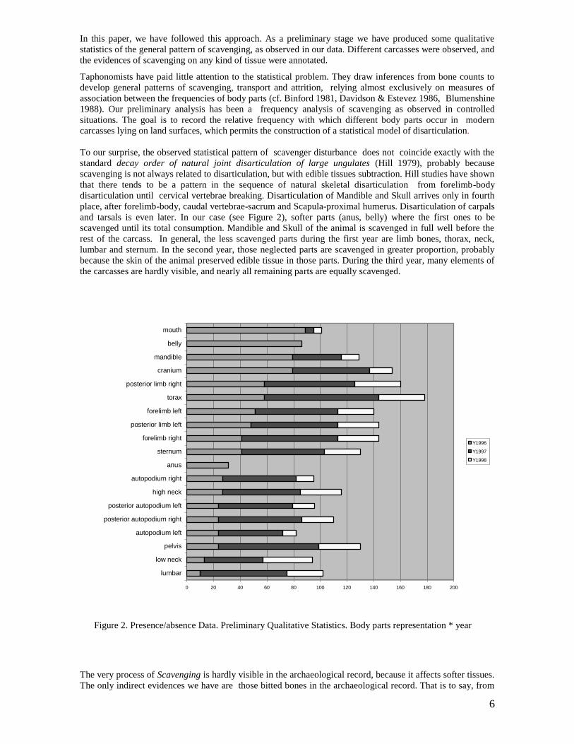
In this paper, we have followed this approach. As a preliminary stage we have produced some qualitative
statistics of the general pattern of scavenging, as observed in our data. Different carcasses were observed, and
the evidences of scavenging on any kind of tissue were annotated.
Taphonomists have paid little attention to the statistical problem. They draw inferences from bone counts to
develop general patterns of scavenging, transport and attrition, relying almost exclusively on measures of
association between the frequencies of body parts (cf. Binford 1981, Davidson & Estevez 1986, Blumenshine
1988). Our preliminary analysis has been a frequency analysis of scavenging as observed in controlled
situations. The goal is to record the relative frequency with which different body parts occur in modern
carcasses lying on land surfaces, which permits the construction of a statistical model of disarticulation.
To our surprise, the observed statistical pattern of scavenger disturbance does not coincide exactly with the
standard decay order of natural joint disarticulation of large ungulates (Hill 1979), probably because
scavenging is not always related to disarticulation, but with edible tissues subtraction. Hill studies have shown
that there tends to be a pattern in the sequence of natural skeletal disarticulation from forelimb-body
disarticulation until cervical vertebrae breaking. Disarticulation of Mandible and Skull arrives only in fourth
place, after forelimb-body, caudal vertebrae-sacrum and Scapula-proximal humerus. Disarticulation of carpals
and tarsals is even later. In our case (see Figure 2), softer parts (anus, belly) where the first ones to be
scavenged until its total consumption. Mandible and Skull of the animal is scavenged in full well before the
rest of the carcass. In general, the less scavenged parts during the first year are limb bones, thorax, neck,
lumbar and sternum. In the second year, those neglected parts are scavenged in greater proportion, probably
because the skin of the animal preserved edible tissue in those parts. During the third year, many elements of
the carcasses are hardly visible, and nearly all remaining parts are equally scavenged.
Figure 2. Presence/absence Data. Preliminary Qualitative Statistics. Body parts representation * year
The very process of Scavenging is hardly visible in the archaeological record, because it affects softer tissues.
The only indirect evidences we have are those bitted bones in the archaeological record. That is to say, from
0 20 40 60 80 100 120 140 160 180 200
lumbar
low neck
pelvis
autopodium left
posterior autopodium right
posterior autopodium left
high neck
autopodium right
anus
sternum
forelimb right
posterior limb left
forelimb left
torax
posterior limb right
cranium
mandible
belly
mouth
Y1996
Y1997
Y1998

7
the total amount of bones in a carcass, only the quantity of bitted bones can be used as evidence of the
intensity of scavenging (Mameli & Estévez, 1999, Estevez & Mameli 2000). The obvious question is then the
relationship between scavenging and morphological damage discovered on the bone surface.
If we consider now the number of bones with traces of animal scavenging (bitted bones)(Figure 3), the results
of our controlled observations suggest that cranium is the only damaged skeletal part in the first year, which
coincide with the fact of preliminary scavenging on less skin protected parts. During the second year, skulls
are still being damaged, together with scapulae, pelvic bones and ribs. Long bones, although scavenged show
very few evidences of surface modification, concentrated on epiphyses. In the third year, vertebrae are the
most damaged bones.
FFiigguurree 33.. BBiitttteedd BBoonneess ddaattaa.. PPrreelliimmiinnaarryy QQuuaalliittaattiivvee SSttaattiissttiiccss.. BBiitttteedd bboonneess rreepprreesseennttaattiioonn ** yyeeaarr
There is also a strong temporal dynamics, which prevent a proper description of the scavenging process from
archaeological remains. If we consider that archaeological record is very similar to our last year observations
–when trapping has already begun-, then we see that most bones are bitted in a similar relative frequency,
with the exception of zigopodia, sternum, ribs. But to affirm that those parts have been less scavenged than
others would be a misleading conclusion, as the results for first and second year suggest.
To go beyond this frequency description we need multivariate techniques to disentangle the multiplicity of
effects produced by different post-depositional processes. We have studied through Correspondence Analysis
the presence/absence of observed evidences for scavenging.

8
-2,94 -2,06 -1,91 -1,20 -0,55 0,19 0,22 0,28 0,46 0,56 0,72 1,13
x
-1,38
-0,48
-0,39
-0,32
-0,29
-0,13
-0,01
0,17
0,39
0,43
0,52
0,81
y
cranium
mouth
mandible
neck
torax
sternum
belly
lumbar
pelvic
anus
limb
feet
Figure 4. Presence/Absence Data. Correspondence Analysis of all carcasses during 3 years of observation.
Variables Plot.
A Bi-dimensional factorial solution accounts for a very low proportion of total variance (42%). That means
that we cannot speak about a general pattern of variation which can explain observed variation among
carcasses. 87 scavenging events have been observed, and it seems impossible to infer a regular pattern (see
Figure 4). Where the anus or belly have been scavenged, other body parts have not evidences of being
disturbed or modified as a result of scavenging. In the opposite, where limb bones or autopodia have been
scavenged, there are no evidences of disturbance in the softer parts.
When we consider all observations made during the three years of the experiment, the only pattern which
emerges is that of the influence of the softer parts scavenging, instead of disarticulation.. In figure 4, it is
interesting to observe the differences and similarities between head parts (cranium, mandible, mouth, even
neck) and limb bones (limbs and feet)
Differences between the theoretical pattern (Hill 1979) and the observed one in our case study is probably the
result of the characteristic of grey foxes scavenging (little canids) and the anatomical features of guanaco,
with very robust bones and a thick skin. We have observed that before disarticulation, little canids ravage soft
tissues from the head of the animal (eyes, tongue, etc.) or the belly. Only when other disturbance process have
acted, meat is easier to scavenge. This is why forelimb bones are mostly scavenged at later moments.
5. THE STATISTICS OF “DEFORMATION” PROCESS: Temporal Dynamics
In most taphonomic analysis of scavenged carcasses, temporal dynamics are only partially taken into account.
We think that it is impossible to understand scavenging as a disturbance process, if we do not characterize it
as a dialectical process, where a non-linear aggregation of quantitative changes, beyond a threshold, produce a
qualitative transformation. That means that a single description of some events of scavenging is not enough
for understanding the process. Scavenging is a dynamic process, introducing quantitative modifications which
eventually produces a deep discontinuity.
Why carcasses with softer parts being scavenged have no evidences of modification in other body parts?
Because scavenging is not a static event, but a continuing process. That means, what is not scavenged at first,
will be ravaged later. We have controlled three temporal stages for each case, and we have documented a
strong temporal component

9
1996 1997 1998
year
-6,00 -4,00 -2,00 0,00 2,00
Dimension 1
-4,00
0,00
4,00
8,00
Dim
en
sio
n 2
Figure 5. Presence/Absence Data. Correspondence Análisis of all carcasses during three years of observation.
Individual Scores with temporal values stratification
An opposition between first year observations, and the rest characteristically dominate dimension 1, which
accounts for 29% of total variance (see Figure 5). If we combine these results with those obtained in
preceding chapter, we can arrive at the conclusion that softer parts are much scavenged during the first year
that later in the process. It is interesting that we cannot separate the last two stages on the basis of softer parts
scavenging.
Let we process the results differentiating the effects for each temporal stage.
Variability among carcass during the first year is very great (Figure 6a). A Bi-dimensional Multiple
Correspondence Analysis only accounts for 36%. The main aspect of this variability is the relevance of low
neck. That means, carcasses with evidence of scavenging at the level of the low neck (4 items), are
significatively different from the others. In general, the same body part seems to be scavenged differently in
different carcasses. During the second year (Figure 6b), the perceived regularity only accounts for 25% of
total variance, but events are totally different. Softer parts have disappeared, and the carcasses become
disarticulated. As a consequence, the same body part is processed in the same way in different carcasses. As
the time goes, the effects of scavenging are more similar, and we can define some redundancy patterns.
During the third year (Figure 6c), most body parts have disappeared, and foxes scavenge all remains they can
find. The overall similarity increases, because the Multiple Correspondence Analysis accounts for 40 % of
total variance.

10
-3,000 -2,000 -1,000 0,000
1996x
-1,00
0,00
1,00
1996y
cranium
mouthmandible
Hneck
Lneck
torax
sternum
belly
lumbarpelvic
anus
forelimb
postlimb
forefeet
postfeet
Figure 6a. Presence/Absence Data. Correspondence Analysis. First year of observations. Variable Plotting
-4,00 -2,00 0,00
1997x
-2,00
-1,00
0,00
1,00
1997y
cranium
mandibleHneck
Lnecktoraxsternum
lumbarpelvic
forelimbpostlimb
forefeetpostfeet
Figure 6b. Presence/Absence Data. Correspondence Análisis. Second year of observations. Variable Ploting
-3,000 -2,000 -1,000 0,000 1,000
1998x
-2,000
0,000
2,000
1998y
craniummandible
Hneck
Lnecktorax
sternum
lumbar
pelvic
forelimbpostlimb
forefeet
postfeet
Figure 6c. Presence/Absence Data. Correspondence Analysis. Third year of observations. Variable Plotting

11
It is highly significative that the important differences between forelimbs and postlimbs, as between left and
right during the first year of observations (Figure 6a), diminish during the second year (Figure 6b). That
means that extremities seem to have been scavenged differently in different carcasses at the beginning of the
process, tending towards an increasing similarity. We can explain all this temporal dynamics suggesting that
the more scavenged the bones, the more disturbance, but also, the more similarity between body parts. The
primary deposition has been totally altered, but similar bones are scavenged in similar ways, when carnivores
have less edible choice, than when carcasses are complete.
We have also studied the influence of the intensity of scavenging. Figure 7 plots factor scores for individual
carcasses against a measure of intensity (number of bones displaced or modified). In all cases, the most
disturbed carcasses (cases where intensity values are the highest) are usually at the center of the distribution,
what suggests the high similarity between them. Most cases of low intensity appear everywhere in the plot,
suggesting the low degree of global similarity between the best preserved carcasses. This pattern is clearer at
later stages than an the beginning of the scavenging process.
0,00 8,50 17,00
intensity
-4,00 -2,00 0,00 2,00 4,00
Dimension 1
-4,00
-2,00
0,00
2,00
4,00
Dim
en
sio
n 2
Figure 7a. Presence/Absence Data. Correspondence Analysis Individual Scores for each carcass during the
first year of observations
0,00 8,50 17,00
intensity
-4,00 -2,00 0,00 2,00 4,00
Dimension 1
-4,00
-2,00
0,00
2,00
4,00
Dim
en
sio
n 2

12
Figure 7b. Presence/Absence Data. Correspondence Analysis Individual Scores for each carcass during the
second year of observations
0,00 8,50 17,00
intensity
-6,00 -4,00 -2,00 0,00 2,00 4,00
Dimension 1
-4,00
-2,00
0,00
2,00
4,00
Dim
en
sio
n 2
Figure7c. Presence/Absence Data. Correspondence Analysis Individual Scores for each carcass during the
third year of observations
Consequently, we cannot conclude that the only effect of scavenging is to increase entropy. In fact, although
disorder increases, the general similarity also increases. This final patterning of animal bones at butchery sites
seem to be very different to the original pattern, which becomes unrecognisable. The more disturbances
scavenging has produced in the past, the less possibilities of differential re-scavenging remains in the present.
Consequently, as the process continues, scavenging concentrates in those bone which survive, appearing some
hints of regular pattern at a later stage. In any case, this pattern does not go beyond 40% of total variance.
Temporal dynamics of scavenging are not characterised by a simple accumulative process from low entropy
sets (death animals) to higher entropy patterns (scavenged carcasses), but it should be defined as a non-linear
aggregate of quantitative changes, which beyond a threshold, produce a qualitative transformation (an
archaeological deposit). We have not identified any regular pattern that could differentiate scavenging from
other social actions, but a general pattern towards increasing qualitative deformation. This result is in strong
opposition with usual approaches trying to identify natural disturbance processes using single identifiers.
THE STATISTICS OF “DEFORMATION” PROCESS: Spatial Dynamics
In our case study, we have discovered evidence for a relationship between the intensity of scavenging, the
distance of transported elements and the relative frequency of lost material: although the intensity of
scavenging diminish as the time goes, the spatial disturbance (distance) increases .
13
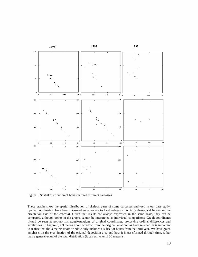
Figure 8. Spatial distribution of bones in three different carcasses
These graphs show the spatial distribution of skeletal parts of some carcasses analysed in our case study.
Spatial coordinates have been measured in reference to local reference points (a theoretical line along the
orientation axis of the carcass). Given that results are always expressed in the same scale, they can be
compared, although points in the graphs cannot be interpreted as individual comparisons. Graph coordinates
should be seen as non-normal transformations of original coordinates, preserving ordinal differences and
similarities. In Figure 8, a 3 meters zoom window from the original location has been selected. It is important
to realize that the 3 meters zoom window only includes a subset of bones from the third year. We have given
emphasis on the examination of the original deposition area and how it is transformed through time, rather
than a general exam of the total distribution (it can arrive until 30 meters).

14
We see that differences are not greater between the second and third year, than between the first and second.
That means, scavenging during the second year is still produced on relatively dense carcasses. Dispersal
seems to be a consequence of long scavenging and not a direct consequence of a single event animal action on
carcasses.
We obtain a new test of the previous hypothesis: as the time goes, the density of locations diminishes and the
spread of bones increases. That is, although scavenging is less intense after the first year, occasional
disturbance produces much more spatial dispersal than original scavenging.
Our analysis pretends to examine if the number and nature of bones in one location have anything to do with
characteristics in a neighbour location through the definition of a general model of spatial dependence. We
usually assume that “everything is related to everything else, but near things are more related than distant
things” (Tobler’s law). This assumption is based on the Neighbourhood Principle, which relates the intensity
of influences converging to a single location from the spatially neighbouring locations. This axiom is not
always true, specially when we deal with natural disturbance processes.
What we are looking is whether the location of individual bones or skeletal parts is homogeneous or
heterogeneous in the area defined by the natural disturbance process. The effects of scavenging as a
disturbance process should be explained in terms of the “influence” an action performed at a location has
over all locations in the proximity. A formation or de-formation process can generate some material effects
(quantitative and/or qualitative changes) around it, or it can prevent that effects of other processes leave
evidences in the same vicinity. Some of the processes acting in the vicinity of the location increase the
probability of some material (observable) effects and decrease the probability of others. The approach here
relies on a prior hypothesis of spatial smoothness, which considers that two neighbouring observations are
supposed to have been more likely originated from the same group than two observations lying far apart.
(Barcelo & Pallares 1998).
This can be easily computed by estimating the spatial probability density function associated to each location.
Given that locations are defined bi-dimensionally, we can calculate an interpolated surface representing the
form of a probability density distribution for two continuous random variables, Cartesian co-ordinates x and y.
The idea is to estimate this 2D dimensional density function, given a sample of known locations, by
estimating the density in that area, the relative frequency of all observations falling in a given interval is
counted. We use Kernel estimation techniques for this task (Baxter and Beardah 1997, Delicado 2000). These
techniques are characterised by the use of a weight function (the kernel function) that permits give more mass
to observed data near the point when the function is estimated.
A preliminary exam of point clouds graphs shows that as the time goes, the material effects of scavenging
(spatial disturbance) increases, the density of bone locations diminishes and the probability of inferring the
correct place for the original deposition of the carcass also diminish. We have translated this information
using a kernel density approximation. The results for carcass Number 1 appear in Figure 9.
Figure 9. Kernel Function interpolation on point cloud for Carcass No. 1

15
Contours in Black corresponds to the probability distribution of first year observations, those in grey to the
second and third year. That is, when animal bones begin to be integrated into what will become an
archaeological record (after trapped in soil) we have a disturbed spatial distribution characterised by its lower
density. Given that that distances among bones have increased, the probability of inferring the original
placement of the carcass diminish: the increase of entropy (disorder) is the cause of an increase in the
ambiguity of the archaeological record. The main effect of scavenging is then a negation of Tobler’s Law: in
an altered context, near skeletal parts are not more related than distant parts. In some cases distant skeletal
parts can even be more related than near bones. The question is then if we can discover any traces of the
original deposition even after post-depositional processes.
We have calculated a general spatial density model for all carcasses in the case study.
Figure 10. Kernel density maps for all carcasses in the sample
We use contour maps, to represent spatial densities. Probability maps should be considered a visual model of
locational features, and not an explanation of spatial causality. Contour maps as those presented here are a
graphical convention for showing changes in the probability of action as a function of disturbances generated
by scavenging at neighbouring locations. Figure 10a shows a density map corresponding to undisturbed or
only partially disturbed carcasses: all bones are in the “correct” place according to the anatomy of the dead
animal, and according to the cause of death. As the time moves on, spatial disturbance increase, and the
density of bones diminish. Fig.10c shows the global density of bone placement after three years of continuing
scavenging. It remains a core area of more dense findings, corresponding to the precise location of the
original action (animal death). It is at this level when we can affirm that the higher the density of findings, the
higher the probability of the original action. We are not calculating the probability of scavenging, but
evaluating the possibilities to infer the original action in the palimpsest generated by post-depositional
processes. Results are clearer if we use a 3D representation of the same kernel filter

16
Figure 11. A 3D view of Figure 10
CCOONNCCLLUUSSIIOONNSS
Usually, archaeologists assume that prehistoric social practices, including procurement, butchering, storage,
cooking and disposal will produce faunal assemblages distinct from those generated by natural processes
(catastrophic death, for instance). However, animal bones found in archaeological conditions have usually
been exposed to a long scavenging process, and characteristics of the original deposition are no more visible..
We have shown that scavenging increases entropy, and we have also shown that the patterning at the end of
the disturbance process may be explained in probabilistic terms.
In this paper we have argued that archaeological assemblages should be regarded as aggregates of individual
elements, interacting with various agents of modification in statistical fashion, with considerable potential for
variation. As a result, what we recover and observe does not proportionately represent each aspect of the prior
behaviour. It is not yet possible to explain scavenging in terms of a regular subtraction process characterized
by a logarithmic reduction of the amount of bones to be scavenged. Consequently it does not exist a simple
rule able to separate the effects of scavenging from primary deposition. Each bone assemblage is a
potentially biased sample drawn from an original population that was itself a potentially biased sample. We
should view these discontinuities not only as sampling biases, but as a discontinuous, and non-linear process:
an increasing skeletal disorganization in terms of taphonomic substraction and spatial disturbance is related
with complex site formation histories.
Therefore, element-abundance data cannot be used in archaeology in a simple way to investigate social
practices, like butchery, carcass-transport decisions, human nutritional needs, activity specialization, discard,
rubbish formation, and so on, without considerations of the specific formation process. Interpreting the
content and frequency of an archaeological assemblage must be grounded in an understanding of both the
social and natural events that have influenced the presence/absence, alteration, and displacement (relative to it
as a primary site of production, use or discard) of its individual components and of the assemblage as a whole.
References
ASCHER, R., 1968, “Time’s arrow and the archaeology of a contemporary community”. In Settlement archaeology,
Edited by K.C. Chang, pp. 43-52. National Press Books, Palo Alto.
BARCELO,J.A., PALLARES,M., 1998, “Beyond GIS: The archaeology of social spaces” Archeologia e Calcolatori
Num. 9, pp. 47-80
BARTRAM. L.E., MAREAN, C.W., 1999, “Explaining the Klasies Pattern: Kua Ethoarchaeology, the Die Kelders
Middle Stone Age Archaeofauna, Long Bone Fragmentation and Carnivore Ravaging” Journal of Archaeological Science
26, pp. 9-29
BAXTER,M., BEARDAH,C.C., 1997, “Some Archaeological Applications of Kernel Density Estimates”, Journal of
Archaeological Science, 24, pp. 347-354.
BINFORD, L.R., 1981, Bones. Ancient Man and modern myths. Academic Press.
BLUMENSHINE, R.J., 1988, “An Experimental Model of the Timing of Hominid and Carnivore Influence on
Archaeological Bone Assemblages” Journal of Archaeological Science 15, pp. 483-502
BRAIN, C.K., 1980, “Some criteria for the recognition of bone-collecting agencies in african caves”. In Fossils in the
Making. Vertebrate Taphonomy and Paleoecology. Edited by A.K. Behrensmeyer and A. Hill University of Chicago
Press, pp.107-130.
CARR, C., 1984, “The Nature of Organization of Intrasite Archaeological Records and Spatial Analytic Approaches to
their Investigation”. Advances in Archaeological Method and Theory. Vol. 7. Edited by M.B. Schiffer. New York,
Academic Press, pp.103-222.
CASTRO, P.V., LULL, MICO, R., 1993, “Arqueología: algo más que Tafonomía”. Arqueología Espacial vol. 16-17, pp.
19-28.
COWGILL, G.L., 1970, “Some sampling and reliability problems in archaeology”. In Archéologie et Calculateurs.
Problèmes Semiologiques et Mathematiques. Colloque International du CNRS. Editions du CNRS, Paris, pp. 161-175.

17
DAVIDSON, I., ESTEVEZ, J., 1986, “Problemas de Arqueotafonomía. Formación de yacimientos con fauna” Quaderns,
1985-1986, Homenaje Dr. J.M. Corominas. Pp. 67-87.
DELICADO,P., 2000, “Statistics in Archaeology:New Directions”. In New Techniques for Old Times. Computer
Applicxations and Quantitative Methods in Archaeology. Edited by J.A.Barcelo, I.Briz and A.Vila. Oxford, ArcheoPress
(BAR Int. Series, S757)
DOMINGUEZ-RODRIGO, M., 1999, “The Study of Skeletal Part Profiles: An Ambiguous taphonomic tool for
archaeology” Complutum 10, 15-24.
EFREMOV, I.A.., 1940 “Tafonomy: a new branch of Paleontology” Pan American Geologist 74, pp. 81-93.
ESTEVEZ, J., 2000, “Aproximación dialéctica a la Arqueología”. Revista Atlántica No. 3. Cádiz (Spain).
ESTEVEZ,J., MAMELI, L., 2000, “Muerte en el Canal: experiencias bioestratinómicas controladas sobre la acción
sustractora de cánidos” Archaeofauna, vol. 9, pp. 7-16.
GIFFORD, D.P., 1981, “Taphonomy and Paleoecology: A Critical Review of Archaeology’s Sister Disciplines. Advances
in Archaeological Method and Theory. Vol. 4. Edited by M.B. Schiffer. New York, Academic Press, pp. 365-438.
HASSAN, F.A., 1987, “Re-Forming Archaeology: A Foreword to Natural Formation Processes and the archaeological
Record”. In Natural Formation Processes and the archaeological Record. Edited by D.T.Nash and M.D. Petraglia.
Oxford, British archaeological Series S352, pp. 1-9.
HILL, A.P. 1979, “Butchery and natural disarticulation: an investigatory technique”. American Antiquity 44, pp. 739-744.
KLEIN, R., 1980, “The interpretation of Mammalian Faunas from Stone-Age Archaeological Sites, with Special
Reference to Sites in the Southern Cape Provincia, South Africa”. Fossils in the Making. Vertebrate Taphonomy and
Paleoecology. Edited by A.K. Behrensmeyer and A. Hill University of Chicago Press, pp.223-246.
LYMAN, R.L., 1987, “Archaeofaunas and Butchery Studies: A Taphonomic Perspective”. Advances in Archaeological
Method and Theory. Vol. 10. Edited by M.B. Schiffer. New York, Academic Press, pp.249-337.
MAMELI,L., ESTEVEZ, J., 1999, “Procesos Post-deposicionales. Un caso de experimentación tafonómica en un área
arqueológica” Reunión de Experimentación en Arqueología. Edited by L. Mameli and J. Pijoan. UAB-Prehistory Series.
“Treballs d’Arqueologia”, Special Issue.
MARCINIAK, A., 1999, “Faunal Materials and Interpretive Archaeology. Epistemology Reconsidered” Journal of
Archaeological Method and Theory No. 6, (4), pp. 293-320
MAREAN, C.W., BERTINO, L.W., 1994, “Intrasite spatial analysis of Bone: subtracting the effect of secondary
carnivore consumers” American Antiquity 59(4), pp. 748-768.
MEADOW, R.H., 1976, “Methodological concerns in Zoo-Archaeology” IX Congress UISPP, pp. 110-123.
MONAHAN, C.M., 1998, “The Hadza Carcass Transport Debate Revisited and its Archaeological Implications” Journal
of Archaeological Science 25, pp. 405-424.
ROGERS, A.R., 2000, “On equifinility in Faunal Analysis” American Antiquity 65(4), pp. 709-723.
SCHIFFER, M.B., 1987, Formation processes of the Archaeological Record. Albuquerque, University of New Mexico
Press.
STAHL, P. W., 1996, “The Recovery and Interpretation of Microvertebrate Bone Assemblages from Archaeological
Contexts” Journal of Archaeological Method and Theory vol. 3 (1), pp. 31-75
STAHL, P.W., 1999, “Structural Density of Domesticated South American Camelid Skeletal Elements and the
Archaeological Investigation of Prehistoric Andrean Ch’arki” Journal of Archaeological Science 26, 1347-1368.
Top Related
Copyright © 2022 FDOKUMEN

