Download - Local Zoning and Environmental Justice: An Agent-Based Model Analysis

Urban Affairs ReviewXX(X) 1 –32

© The Author(s) 2013Reprints and permissions:

sagepub.com/journalsPermissions.nav DOI: 10.1177/1078087413505736

uar.sagepub.com

Article

Local Zoning and Environmental Justice: An Agent-Based Model Analysis

Heather E. Campbell1, Yushim Kim2, and Adam Eckerd3

AbstractThis article presents an agent-based computational analysis of the effects of externality zoning on environmental justice (EJ). We experiment with two ideal types of externality zoning: proactive and reactive. In the absence of zoning, environmental injustice emerges and minority agents have lower average environmental quality than majority agents. With proactive zoning, which allows polluting firms only in designated zones, EJ problems are less severe and appear more tractable. With reactive zoning, which creates buffering zones around polluting firms, environmental injustice tends to emerge more quickly as compared with proactive zoning but tends to decline over time. This analysis examines a possible policy tool available for cities to ameliorate environmental injustice.

Keywordszoning, environmental injustice, agent-based model

1Claremont Graduate University, CA, USA2Arizona State University, Phoenix, USA3Virginia Polytechnic Institute and State University, Alexandria, USA

Corresponding Author:Heather E. Campbell, Department of Politics and Policy, Claremont Graduate University, 170 E Tenth Street, Claremont, CA 91711, USA. Email: [email protected]

XXX10.1177/1078087413505736Urban Affairs ReviewCampbell et al.research-article2013

2 Urban Affairs Review XX(X)

IntroductionFor decades, the environmental justice (EJ) literature has found significant evidence indicating that, after controlling for income and other factors, racial and ethnic minority residents are often disproportionately affected by envi-ronmental disamenities (e.g., Bullard 1990; Campbell, Peck, and Tschudi 2010; Hamilton 1995; Kriesel, Centner, and Keeler 1996; Pastor, Sadd, and Hipp 2001; Ringquist 2005). However, the EJ literature has been so focused on determining whether minority-based environmental injustice really exists that it has been limited in tackling what types of social behaviors and institu-tional structures could combine to lead to the frequently observed minority-disproportionate EJ outcomes (Bowen and Wells 2002; Noonan 2008). Must the observed variation in environmental risk be due to specifically prejudiced goals by decision makers, as some have argued, and as policy has often implicitly assumed? Or are there other social processes that can inadvertently lead to environmental injustice (Pulido 2000; Saha and Mohai 2005)? If we do not understand what parts of the complex social interactions involved in environmentally relevant policy lead to environmental injustice, it is difficult to properly target policy change for better social outcomes.

Besides a malicious intention of firm decision makers in siting (the inten-tional model of EJ) (Pulido 2000; Downey 1998), at least three other compet-ing but nonexclusive explanations of EJ outcomes have been discussed: market dynamics, political power, and local land-use policies (Hamilton 1995; Saha and Mohai 2005). In the market-based view of environmental inequity, the goal of firms is conceived to be maximizing profits and mini-mizing costs. Firms seek to locate where the price of land is cheap and mate-rials are nearby. In this view, environmental inequity is explained because the places where minorities or the poor live coincidentally satisfy such condi-tions better than areas with a higher proportion of the majority or the rich (Been and Gupta 1997). Still within the market-based model, another possi-bility is that minorities, who are disproportionately poorer, might move to areas where polluting firms locate to gain job opportunities (Pastor, Morello-Frosch, and Sadd 2005) or because the polluting firm causes nearby land values to decline. Because minorities are disproportionately poor, this social process can lead to the disproportionate collocation of firms producing envi-ronmental disamenities with minority residents. On the other hand, Hamilton (1995) added the important insight that just measuring economic factors alone was insufficient since political factors—and in particular factors related to the ability to engage in collective action—matter, too. Hamilton’s study operationalized the role of collective action through a voter turnout variable.

These first two explanations, based on market and political rationality of firms, have a long history of empirical examination in EJ (Been and Gupta

Campbell et al. 3

1997; Hamilton 1995; Kriesel, Centner, and Keeler 1996). Besides these two explanations, there are some studies that investigate the link between collec-tive action on local land-use decisions, usually focusing on “Not in My Back Yard” (NIMBY) action, and the potential of powerful actors to keep undesir-able land uses out of high-status communities (Dear 1992; Kraft and Clary 1991; McAvoy 1998; Saha and Mohai 2005).

However, there is limited research on the role of the local land-use struc-tures themselves in EJ outcomes (Maantay 2002). This is surprising, given the widespread awareness of the NIMBY phenomenon, and also considering that efforts to address the EJ problem have been developed by focusing on the spatial distribution and collocation of environmental disamenities and low–socioeconomic-status populations (Been and Gupta 1997). An exception to this general lack of focus on land-use structures is Boone and Modarres (1999), which uses historical analysis to understand the current dispropor-tionate collocation between high levels of pollution and Latina/o residents in the City of Commerce, finding an important effect of land-use planning and zoning decisions.

Most American cities utilize some set of zoning mechanisms to regulate local land use. Local zoning organizes and sets boundaries on the siting deci-sions of firms and residents in cities. Since land-use structure plays a role in shaping spatial patterns in cities, and Boone and Modarres (1999) find evi-dence of its importance in their case study, its relation to EJ outcomes requires further attention, especially because it has potential as an EJ policy lever for local governments.

In the research presented here, we elaborate further on the relationship between EJ and land-use zoning systems. We model an artificial city in which residents and firms dynamically interact in terms of their siting decisions, and we explore the environmental consequences. Within this framework of dynamic interaction, zoning rules are added to experiment with their effects on residents’ exposure to environmental harm. Through this effort, we can assess the difference, if any, that zoning can have on EJ outcomes, and pose hypotheses for future empirical assessments of local land-use planning and EJ outcomes. We focus on two primary contrasts: (1) EJ outcomes without versus with zoning and (2) EJ outcomes using a proactive versus a reactive zoning policy.

Why Local Zoning in EJ Research?

Local Zoning in the United StatesIn the United States, local zoning is a common tool of land-use policy (Fischel 1997). It has been used for various purposes such as promoting economic


development and sheltering residential populations from industrial disameni-ties; the latter is often called externality zoning. Boone and Modarres (1999) find evidence that zoning in the Los Angeles area was seen as a means of separating “residences away from industry for the benefit of both parties” (p. 180). Removing residences from industrial areas “protected them [industries] from damage and nuisance suits, as well as injunctions” (Boone and Modarres 1999, p. 180).

Zoning restrictions can be articulated in two ways: First, when certain uses are omitted from the description of a particular zone, such a use is prohibited in that zone; second, a zone’s description can explicitly prohibit a particular use. For example, “R zones” refer to residential zones, and R zone codes can include details of permitted uses such as single-family residences, allowed lot sizes, and so on. R zones can be further classified as R-1, R-2, R-3, and so forth, with different permitted residential uses, and the lower number zones can be logically nested within higher ones. In other words, R-2 can include permitted uses for R-1 zones plus additional uses. R-3 includes R-2 uses and additional uses, and so on. Similarly, “C zones” specify commercial uses, and some uses permitted in R zones can also be nested within C zones (creating mixed-use zones). “M zones” or “I zones” specify manufacturing or indus-trial uses. They may explicitly say that residential uses are not permitted; simplified code examples are noted by Woodworth, Gump, and Forrester (2006, pp. 166-70). While zoning is one of the most widely used local land-use regulations, there are localities that experiment with an unregulated form and have no explicit zoning regulations. With a strong free-market predilec-tion, for example, Houston, Texas, is the largest U.S. city without zoning (Qian 2011). However, even in Houston, rather than a pure open market, other land-use control mechanisms such as homeowner associations and deed restrictions are used to segment land uses (Qian 2011).1

Some argue that zoning can be used for the invidious purpose of segrega-tion—or historically was—which could create path dependencies that explain some current inequities. The exclusionary rationale for zoning refers to “a deliberate desire to exclude lower-income and/or minority households from the jurisdiction” (Ihlanfeldt 2004, p. 273). Exclusion can be based strictly on racial prejudice or use of race as a proxy for neighborhood quality—for example, for fiscal purposes. Two very early examples that illustrate this zon-ing idea date from 1885, when San Francisco prohibited laundries in residen-tial areas, and 1916, with New York City’s Zoning Resolution (Wilson, Hutson, and Mujahid 2008). It is argued that both had an exclusionary intent to segregate certain social groups: the former attempted to restrict Chinese people from living in white neighborhoods, and the latter created an exclu-sive zone to “keep the immigrant factory workers out of sight of the wealthy women shopping on Fifth Avenue” (Maantay 2002, p. 577). Although zoning

Campbell et al. 5

can be created solely for a fiscal purpose (Fischel 1992), some argue such use inevitably has an exclusionary implication for certain social groups. That is, fiscal zoning may attract property owners with high tax-to-service ratios, and thus exclude the poor or the racial minorities who might reduce property values in exclusive residential areas (Pogodzinski and Sass 1991).

Others argue that zoning can be beneficent, intended to separate citizens from negative externalities of production, with an unintended consequence of housing markets responding accordingly, which causes segregation by eco-nomic status. The rationale of externality zoning is to minimize the impact of production externalities on residents by separating incompatible land uses (i.e., residential, commercial, and industrial). For example, waste-related facilities can only be sited in areas designated as M zones, intending to reduce harm to residents. However, Maantay (2002) argues that noxious uses tend to be concentrated in poor and minority areas “due to the re-zoning of more affluent and less minority industrial neighborhoods to other uses” (p. 583). In a review of empirical studies that examine these rationales,2 Ihlanfeldt (2004) concludes that, while there is a paucity of evidence on the motive of zoning, “there is consensus across studies that fiscal considerations frequently moti-vate restrictive land-use regulations. Evidence on the externality and exclu-sionary motives, on the other hand, is mixed across studies” (p. 275). It is not easy to separate these motives of local planners or localities as they make zoning decisions, and they most likely are intertwined to some degree.

As early as 1968, though critical of what it saw as emerging misuses of zoning, the American Society of Planning Officials stated, “zoning has done much more good than harm” (Lazero 1971, p. 160). Schilling and Linton (2005) argue that

The exclusion of intensive industrial and commercial uses has undoubtedly improved the quality of life in many communities. . . . [But] Zoning is still subject to considerable tensions involving social and environmental justice, such as the disproportionate number of waste production and waste-disposal uses in districts bordering or including poor residential populations. (pp. 100-101)

However, in the urban studies literature, zoning has gained much schol-arly attention due to the argument that it excludes lower income households from suburban communities by artificially inflating the cost of housing (Ihlanfeldt 2004). A large number of studies, thus, have examined the impact of urban zoning regulations on housing market inflation (e.g., Pogodzinski and Sass 1991), income/racial segregation (i.e., Pendall 2000; Rothwell and Massey 2009), or imbalance in the labor market (e.g., Richardson et al. 1993). In this context, it is worth noting that Ohls, Weisberg, and White (1974) argued that “it is not generally possible using a priori theory to predict”


whether either externality zoning or fiscal zoning will increase or depress “aggregate land value in a community” (p. 428).

While limited, there is some research that explicitly analyzes the connec-tion between land-use control through zoning and EJ outcomes (e.g., Maantay 2002; Wilson, Hutson, and Mujahid 2008). Since zoning regulates land-use types and densities, intentionally or not it also governs potential environmen-tal impacts on populations in zoned areas. As mentioned, zoning may specify the siting of noxious uses within certain areas, but, depending on where those areas are, it can also contribute to the disproportionate burden of environ-mental and health impacts on certain social groups (Maantay 2002; Schilling and Linton 2005). Thus, Maantay argues that zoning has an inevitable con-nection to environmental injustice, but the underlying zoning designations and subsequent changes have not been properly factored into EJ analysis (2002). Even now the critique remains valid except for a few studies (e.g., Pastor, Morello-Frosch, and Sadd 2005) that explicitly include land-use vari-ables in their empirical EJ research. Pastor, Morello-Frosch, and Sadd (2005) found a racially disparate pattern of cancer risks associated with air toxics even when income and land-use variables were included. Our study comple-ments Pastor et al.’s cross-sectional analysis by examining dynamics of an EJ quality gap under different zoning scenarios.

It is important to keep in mind that the motives and consequences of zon-ing may be separate. Furthermore, neither the motives of zoning nor its con-sequences for EJ outcomes are yet clear. Zoning, whether done for beneficent or malicious purposes, can create both negative and positive externalities within complex social systems that include interrelated and interdependent heterogeneous entities. Without much empirical literature base to draw from, we do not have specific expectations with regard to the empirical relationship between zoning and environmental justice outcomes. A case could be made that zoning contributes to environmental injustice by establishing the institu-tional rules whereby lower socioeconomic status groups tend to cluster near noxious facilities (Pulido 2000), but a case could also be made that one of the original intents of zoning was to protect residents from noxious facilities and that zoning, thus, ought to alleviate environmental injustice. Using a compu-tational simulation approach, we aim to draw some insight into previously unconsidered hypotheses for empirical testing on externality zoning and environmental injustice in U.S. cities and municipalities.

Use of Agent-Based Modeling for Land UseSimulation using agent-based modeling (ABM) allows us to create an artifi-cial society within which firms, residents, and government actions can be introduced and examined in an experimental setting, enabling us to control

Campbell et al. 7

for external effects while maintaining complexity within the model itself (Epstein 2006; Gilbert 2008). In what is generally considered the first con-ceptual ABM, Thomas Schelling (1971) demonstrated that residential segre-gation could arise even when every actor in the simulation was, though race-conscious, not racist. This first ABM, though quite simple, demonstrated the power of emergent social outcomes and the possibility that they could be unintended by every actor. With advances in computing technology, it has become easier to explore and experiment with complex social processes that involve autonomous and heterogeneous actors and their interdependencies and interactions. Thanks to the flexibility and applicability of this simple foundation, ABM has been used for studying important urban policy con-cepts (Desai 2012; Epstein 2006; Tesfatsion and Judd 2006).

For example, the use of ABM in the study of land-use and land-cover change (LUCC) has been rapidly growing (Parker et al. 2003). The basis of the LUCC models is to understand land as “a dynamic canvas on which human and natural systems interact” (Parker et al. 2003, p. 314) and to exam-ine spatial patterns (e.g., urban sprawl) that emerge from human behavior as an action or reaction to changes in the environment. Some explicitly deal with zoning as an important component of the LUCC models (Ligmann-Zielinska and Jankowski 2010; Zellner et al. 2009, Zellner et al. 2010). Zellner et al. (2010) examined the combined effects of zoning and residents’ density preferences on urban sprawl patterns and utility distribution among residents. In their model, the utility of each cell is decided by cell density, distance to service centers, and aesthetic quality. The study reports that zon-ing can reduce sprawl, but in return it decreases average utility and increases inequality of utility among residents. However, environmental injustice has not been a focal point of these LUCC models. With EJ perspectives not inte-grated with these models, this paper addresses this gap and contributes to our understanding of EJ by analyzing zoning and EJ together in a dynamic urban setting, using ABM.

The EJ ABM we present here is different from Zellner et al. (2010) in that heterogeneity in social groups, not just in preferences, is a starting point of the model. Residents have a preference for racial/ethnic similarity of neigh-bors that constrains their residential choice. The final residential choice deci-sion is made based on the utility of a location, where utility consists of environmental quality, price, and proximity to the nearest firm. In addition, we set up zoning mechanisms differently from Zellner et al. (2010). While in the Zellner et al. model, zoning reflects a developer’s decision to respond to the demand of a portion of the population, we conceptualize zoning as a local government’s action to prevent or correct market inefficiency through exter-nality zoning. This allows us to explore plausible local policy as a means of improving environmental justice.


Modelling Local Zoning Decisions in an EJ ABM

The Landscape and Model SummaryThe landscape consists of a 101 × 101 grid of cells (10,201 plots of “land”). Each cell is defined by (x, y) coordinates. In the landscape, each 10 × 10 set of plots is defined as a block, and transportation routes run between the blocks. Thus, each block contains 100 plots, and 100 blocks exist in the land-scape. The blocks can be viewed as proxies for neighborhoods or for Census Block Groups. Plots have three key attributes: environmental quality, price, and proximity to firms. Each of the plots within a block is initially homoge-neous with respect to environmental quality. The expected quality value of each plot is initialized with a value of 50. On the other hand, the price of each plot is initially determined through a random assignment of value, mirroring median home prices in the United States. Each plot value is derived from a normal distribution with a mean of US$173,000 and a standard deviation of US$34,000 ( U.S. Census Bureau 2010). Firm and resident agents will reside in the landscape (see “The Agents” section for details). New residents are introduced to the landscape following a population growth function. When there is excess labor supply, a new firm is established, and each plot updates its proximity to the nearest firm based on the Euclidean distance. At each step, these three attributes determine a utility score for each plot (see the “Residential Choice” section below). As discussed further later, firms may be of two types: those that produce high levels of pollution, which are disameni-ties, and those that produce jobs with no or low levels of pollution. Because people and cities value jobs, the latter are considered amenities.

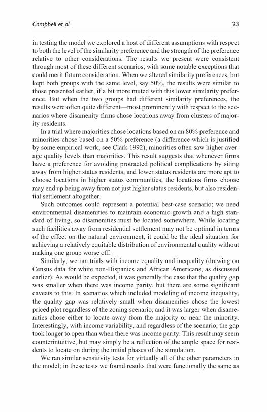
Zoning ScenariosZoning is the crucial part of the landscape in this simulation. The base model runs without zoning, mimicking a pure market scenario. Then, we introduce two externality-zoning scenarios as types of local government policy action: proactive zoning and reactive zoning. For the proactive zoning scenario, the following procedure was developed. At the beginning of the simulation, approximately 10 blocks are randomly selected to be zoned, with half defined as industrial zones (M zones) and the other half as commercial zones (C zones). Using a stochastic distance function, the zones are then expanded outward from each of these blocks, with the end result consisting of randomly sized clusters of zoned blocks. The rest of the plots are then open to residen-tial settlement (similar to R zones). Once the M or C zones are set, new disa-menities must locate in industrial zones, and new amenities must locate in commercial zones. In one set of proactive scenarios, residents can only locate

Campbell et al. 9

in residential zones; in another set, mixed use of land is allowed, and resi-dents can locate in C zones.

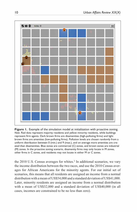
In the second set of experiments, zones are created reactively throughout the simulation after certain conditions are satisfied with respect to the loca-tions that firms have selected. When a block has more than two environmen-tal disamenities, the block becomes M-zoned (industrial). If resident agents already occupied plots in the zone just created, they must relocate to other nonzoned plots (in accordance with the standard residential location deci-sions). The same logic is applied to environmental amenities and the creation of commercial zones (C zones). Once commercial or industrial zones are created, new firms must locate in an appropriate zone, as long as the zones have not reached their maximum capacity of firms (i.e., five firms per zoned block), while still maximizing utility from among allowed sites within the zones based on the firms’ siting decision scenarios. If there are no zoned spaces available, firms may locate on any plot that is not occupied, following the siting process described below. Environmental disamenity firms cannot locate in C zones, and environmental amenity firms cannot locate in M zones, although neither type of firm is forced to move if its plot subsequently gets zoned to a nonconforming zone. See Figure 1 for the simulation landscape, and Table 1 for the zoning rules.

The AgentsThe two basic agent types in the models are firms and residents. When a firm or resident enters the landscape, it takes up one plot. Once a plot is occupied, it is unavailable for new firms or residents. The residents-to-firm ratio is set to 50:1 for the base model. The simulation is initialized with 200 residents and thus approximately four firms. All firms provide a benefit (jobs) and a cost (pollution). It is assumed that all firms are the same in terms of the desir-ability and number of jobs they provide. When a firm is introduced to the landscape, the levels of pollution are randomly assigned as integers between zero and nine inclusive (a uniform distribution), with firms that produce sub-stantial pollution (greater than 5 on this scale) categorized as environmental diamenities and those with lower levels of pollution defined as environmen-tal amenities. Thus, approximately 40% of firms are disamenities and the remaining firms are amenities.

The landscape also contains resident agents that are defined as “majority” or “minority,” indicating two hypothetical races. The simulation begins with more majority than minority residents: 70% to 30% (140 majorities and 60 minorities). Within these subgroups, the resident agents are assigned differ-ential incomes. In the base scenarios, each agent in each racial group is ran-domly assigned an income from a normal distribution roughly approximating


the 2010 U.S. Census averages for whites.3 In additional scenarios, we vary the income distribution between the two races, and use the 2010 Census aver-ages for African Americans for the minority agents. For our initial set of scenarios, this means that all residents are assigned an income from a normal distribution with a mean of US$54,000 and a standard deviation of US$41,000. Later, minority residents are assigned an income from a normal distribution with a mean of US$32,000 and a standard deviation of US$40,000 (in all cases, incomes are constrained to be no less than zero).

Figure 1. Example of the simulation model at initialization with proactive zoning.Note. Red dots represent majority residents and yellow minority residents, while buildings represent firm agents. Dark brown firms are disamenities (high-polluting firms) and light brown firms are amenities (low-polluting firms). Pollution levels are chosen randomly from a uniform distribution between 0 (min.) and 9 (max.), and on average more amenities are cre-ated than disamenities. Blue zones are commercial (C) zones, and brown zones are industrial (M) zones. In the proactive zoning scenario, disamenity firms may only locate in M zones, other firms in C zones, and residents may not locate in either M or C zones.

Campbell et al. 11

To represent a growing urban region, the population growth rate is set to 5% during the simulation. That is, some resident agents are “born” and “die” over time such that the net rate of population growth is 5%.4 At each step, new residents numbering 7% of the current population are “born.” In words, 7% of the existing resident agents are asked to replicate themselves. The “death” procedure starts to work after the population reaches 500. The oldest 2% of the existing population “die” and their plots open up for new use. If there is not a clear set of 2% of the agents who have been in the simulation, the longest length of time, agents are selected randomly from those tied as oldest. This process keeps the demographic split at roughly 70% majority and 30% minority, with some random variation.

Firm SitingA key behavior occurs during the simulation: both firms and residents seek satisfactory plots upon which to settle. When there is an unmet demand for jobs due to population growth, a new firm is introduced to the landscape. A new firm’s siting decision is based on two steps. First, agglomeration econo-mies are modeled (Krugman 1993). Previous empirical studies have shown that preexisting disamenities matter in explaning other disamenities’ location decisions (Bowen, Atlas, and Lee 2009; Campbell, Peck, and Tschudi 2010;

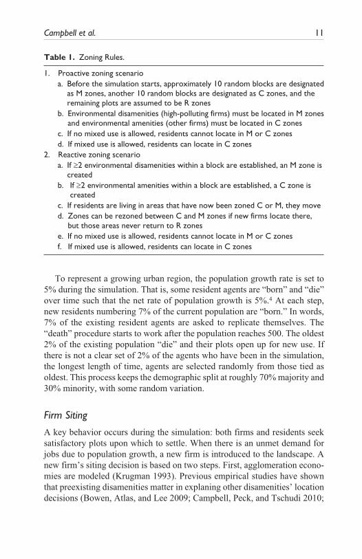
Table 1. Zoning Rules.

1. Proactive zoning scenario a. Before the simulation starts, approximately 10 random blocks are designated

as M zones, another 10 random blocks are designated as C zones, and the remaining plots are assumed to be R zones

b. Environmental disamenities (high-polluting firms) must be located in M zones and environmental amenities (other firms) must be located in C zones

c. If no mixed use is allowed, residents cannot locate in M or C zones d. If mixed use is allowed, residents can locate in C zones2. Reactive zoning scenario a. If t2 environmental disamenities within a block are established, an M zone is

created b. If t2 environmental amenities within a block are established, a C zone is

created c. If residents are living in areas that have now been zoned C or M, they move d. Zones can be rezoned between C and M zones if new firms locate there,

but those areas never return to R zones e. If no mixed use is allowed, residents cannot locate in M or C zones f. If mixed use is allowed, residents can locate in C zones


Wolverton 2009). Therefore, with no zoning, firms are modeled as preferring to be near firms like themselves but with no more than five firms allowed within any one block. In other words, a firm prefers plots where there is at least one other of the same type of firm within 10 concentric rings5 and blocks that have less than five firms. If there is no other firm of the same type, the firm considers plots that have less than five firms of any type as candidate plots.

With zoning scenarios, the firm considers zone types given its own cate-gory as a disamenity or an amenity and also the number of firms settled within each block (again, firms prefer blocks that have less than five firms). Second, after the agglomeration condition is satisfied, firms make their siting decisions based on their plot-selection criteria. Amenities always seek the lowest priced plot. Disamenities make choices under one of three different scenarios: (1) choose the lowest priced plot, (2) purposely choose plots near minorities, or (3) choose plots away from majorities (see Eckerd, Campbell, and Kim 2012, for details). After siting, firms do not move and are not removed during the simulation. See Table 2 for a description of the siting rules.

Once a firm’s siting decision is made, disamenities degrade the environ-mental quality of a plot, while amenities improve the quality of a plot. We model these environmental effects in two ways: first, as a reflection of the pollution variable associated with the focal firm, and second, as a function of spatial proximity. If a new disamenity is introduced to a plot during the simu-lation, the quality value of the plot upon which the disamenity is located decreases, reflecting the disamenity’s pollution level (between 6% and 9%). That is, if a new disamenity with a pollution level 6 is sited on a plot, the quality of the plot is reduced by 6% of the previous quality value. The higher

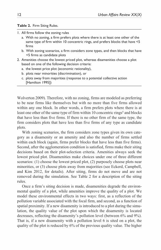
Table 2. Firm Siting Rules.

1. All firms follow the zoning rules a. With no zoning, a firm prefers plots where there is at least one other of the

same type of firm within 10 concentric rings, and prefers blocks that have <5 firms

b. With zoning scenarios, a firm considers zone types, and then blocks that have <5 firms as candidate plots

2. Amenities choose the lowest priced plot, whereas disamenities choose a plot based on one of the following decision criteria:

a. the lowest price plot (economic rationality), b. plots near minorities (discrimination), or c. plots away from majorities (response to a potential collective action

[Hamilton 1995])

Campbell et al. 13

the pollution level, the larger the reduction. The quality of all plots within the block where the disamenity is located also decreases, again depending upon the disamenity’s pollution level (by between 3% and 5%).

Conversely, if an amenity is introduced to a plot, the quality increases, but the increase is constrained by the amenity’s pollution level. Thus, quality can increase by 5% for a firm with a pollution value of 0, and not increase at all for a firm with pollution level 5 (but quality also does not decrease). The quality of neighbor plots within the block also increases via the same mecha-nism as the decrease associated with disamenities (by between 3% and 0%). These quality operations that are related to the pollution level of the focal firm occur at only one time: the time period after each new firm is introduced to the landscape.

Once the simulation starts, two other procedures influence the quality of plots on an ongoing basis. The quality of each plot at time t is updated from the previous quality at t− 1: negatively adjusted by an inverse distance to the nearest disamenity (Equation 1) and then positively adjusted by an inverse distance to the nearest amenity (Equation 2):

q q dj t j t jk t, , ,( /= ⋅ −−1 1 1 δ (1)

q q dj t j t jk t, , ,( / )= ⋅ +1 1 δ (2)

where qj,t is the quality of plot j at time t, qj,t−1 is the quality of plot j at time t − 1, djk,t is the Euclidean distance from plot j to the nearest disamenity (1) or amenity (2) at time t, and δ, a distance weight to the nearest disamenity or to the nearest amenity, is set to 1.5. In other words, the environmental quality of each plot at each simulation step is decided after adjusting the previous quality with the two sequential calculations.

After Adjustments 1 and 2 occur, quality changes spread out via a spatial decay function, with decreased force based on distance, to adjacent plots (Parker and Meretsky 2004). Each plot diffuses its quality value to the eight neighboring plots based on a diffusion rate. Here the diffusion rate is set to 0.7, so each plot gets one-eighth of 70% of the quality value from each neigh-boring plot. The quality update and diffusion procedures operate at every simulation step.

Residential ChoiceWhen new residents are introduced to the world, their location choices are constrained by their incomes and similarity preferences. Reasoning that wealthy residents will not always opt to select the lowest priced home because it may be located in an undesirable neighborhood, no resident agents will


consider a plot that is less than twice its income level, and given the con-straints preventing the purchase of a home that is out of one’s price range, residents also exclude any plot with a price greater than three times their income level (Parker and Filatova 2008). If there is no candidate plot within their housing price range, any plots priced with less than three times their income level are considered as candidates. If there is no such plot either, then candidate plots are empty residential plots. Once residents find candidate plots that satisfy their income constraints, the similarity preference for living near other residents like themselves is considered (Clark 1992; Schelling 1971). If residents have a similarity preference, they first look for any avail-able plots in their income-constrained decision sets that meet their similarity preference criterion. For example, if the similarity preference for minority is set to 80%, minority agents will only consider locating on plots where at least 80% of the agents on neighboring plots are also minorities. If there are no plots within the affordable price range that meet the residential similarity preference, residents select the plot within the candidate plot set that best matches the utility score described below, regardless of the demographic makeup of the surrounding area.

These income and similarity preference constraints limit residential choice sets; after the constrained set of plots has been identified, residents pick a plot that maximizes their utility within their choice set given each plot’s price, quality, and distance to the nearest job (cf. Brown and Robinson 2005; Pratt 1964; Rand et al. 2002). In other words, within the confines of the income and similarity constraints, residents make a residential decision using a utility score of candidate plots. Utility scores are calculated using the following criteria: low price, high quality, and nearness to place of work, as described in the following equation:

u p q dj t j t j t jk t, , , .= ⋅ ⋅− −α β γ (3)

where the utility score of a plot j at time t is a function of the price and quality of j and distance between the plot j and the nearest job, k, all at time t. The quality of plots at each time is decided following the procedures described in the “Firm Siting” section.

Similar to the environmental quality update procedures, the price of a plot at time t is updated from two sequential procedures at each time. At every time step, the price of each plot is updated from the previous price, negatively adjusted by an inverse distance to the nearest disamenity and then positively adjusted by an inverse distance to the nearest amenity. And then, the prices at time t are altered based on the income level of the resident agents that settle nearby (surrounding eight neighboring plots). First, a multiplier is calculated

Campbell et al. 15

by comparing the difference between twice the average income of nearby residents and the current plot price. If the average income level of residents on the eight neighboring plots, adjusted by the multiplier, is higher (lower) than the price of the plot calculated from the previous procedure, the plot price increases (decreases). Finally, the distance to the nearest (any) firm is used to calculate the utility score. An equal weight of 0.5 is set for the three decision variables. Residents choose a plot with the highest utility score from the choice sets.

As explained, the residential choice of a plot is influenced by price, but each residential plot choice also influences the price of neighboring plots. At each time step, price changes spread out, with decreased force based on dis-tance, to adjacent plots. Each plot diffuses its price value to the eight neigh-boring plots based on a diffusion rate. Here, the diffusion rate is set to 0.7, so each plot gets one-eighth of 70% of the price value from each neighboring plot at every simulation step. It is assumed that once residents locate, they will not move to other locations unless forced to by a zoning change.6 See Table 3 for the residential choice rules and Table 4 for a full description of the model’s parameters.

Environmental Justice Outcomes and Key ScenariosOur key measure of interest is the disparity (if any) in average majority and minority residents’ exposure to environmental risk. To have a sufficient num-ber of trials while still utilizing available computing resources as efficiently as possible, we ran each distinct simulation 200 times, with each simulation run consisting of 70 total steps. For each step in each simulation, we collected the average environmental quality for plots that contained majority residents (Qmi ) and for plots that contained minority residents (Qma ), which are a result of their location choices and firms’ siting decisions. Using this infor-mation, we also calculated an environmental quality gap (QG ) between the

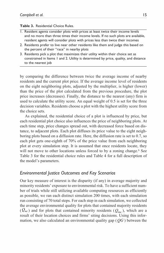
Table 3. Residential Choice Rules.1. Resident agents consider plots with prices at least twice their income levels

and no more than three times their income levels. If no such plots are available, resident agents will consider plots with prices less than twice their incomes

2. Residents prefer to live near other residents like them and judge this based on the percent of their “race” in nearby plots

3. Residents pick a plot that maximizes their utility within their choice set as constrained in Items 1 and 2. Utility is determined by price, quality, and distance to the nearest job


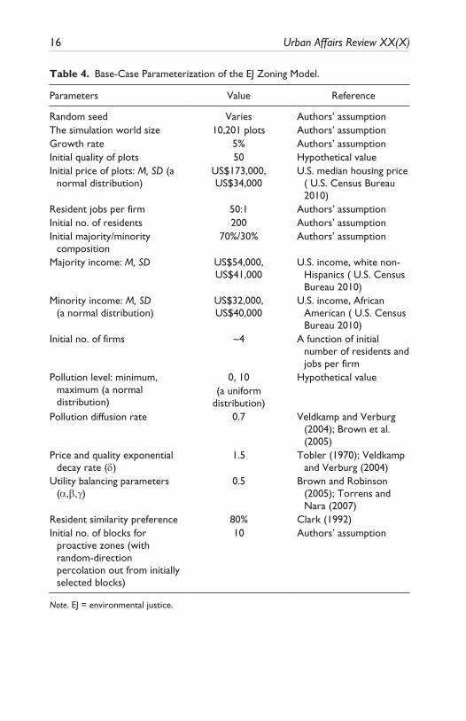
Table 4. Base-Case Parameterization of the EJ Zoning Model.

Parameters Value Reference

Random seed Varies Authors’ assumptionThe simulation world size 10,201 plots Authors’ assumptionGrowth rate 5% Authors’ assumptionInitial quality of plots 50 Hypothetical valueInitial price of plots: M, SD (a

normal distribution)US$173,000, US$34,000

U.S. median housing price ( U.S. Census Bureau 2010)

Resident jobs per firm 50:1 Authors’ assumptionInitial no. of residents 200 Authors’ assumptionInitial majority/minority

composition70%/30% Authors’ assumption

Majority income: M, SD US$54,000, US$41,000

U.S. income, white non-Hispanics ( U.S. Census Bureau 2010)

Minority income: M, SD (a normal distribution)

US$32,000, US$40,000

U.S. income, African American ( U.S. Census Bureau 2010)

Initial no. of firms ~4 A function of initial number of residents and jobs per firm

Pollution level: minimum, maximum (a normal distribution)

0, 10 Hypothetical value(a uniform

distribution)

Pollution diffusion rate 0.7 Veldkamp and Verburg (2004); Brown et al. (2005)

Price and quality exponential decay rate (G)

1.5 Tobler (1970); Veldkamp and Verburg (2004)

Utility balancing parameters (D�E�J)

0.5 Brown and Robinson (2005); Torrens and Nara (2007)

Resident similarity preference 80% Clark (1992)Initial no. of blocks for

proactive zones (with random-direction percolation out from initially selected blocks)

10 Authors’ assumption

Note. EJ = environmental justice.

Campbell et al. 17

resident types (QG = Qma − Qmi). An environmental quality gap score of 0 indicates that there is no difference between the groups. The higher the score, the greater the difference between majority and minority quality. A negative score indicates that minority quality is higher than majority quality.

As we described in the section on modeling, the ABM includes compli-cated location decision-making processes of each agent type (firms, resi-dents, and the local zoning authority). Key scenarios on which this article focuses are three zoning scenarios: (1) no zoning, (2) proactive zoning, and (3) reactive zoning. Within each of these, disamenity firms can site based on one of three decision scenarios: (1) low price (economically rational), (2) sit-ing away from majority concentrations (politically rational), and (3) siting near minority concentrations (discriminatory). Our key research question is how the environmental quality disparity between majorities and minorities occurs under these different zoning and disamenity siting decision conditions.

For the base set of analyses, all residents’ similarity preferences are set at 80%, and it is initially assumed that there is no difference of wealth distribu-tions between the majority and minority. Therefore, the base analyses gener-ate approximately 126,000 observations arising from 9 distinct scenarios × 200 runs per scenario × 70 simulation steps per run. In addition, we ran extra simulations to examine the effect of mixed-use C-zones under proactive or reactive zoning, differential similarity preferences between majorities and minorities, and differential income levels between majorities and minorities.

Results

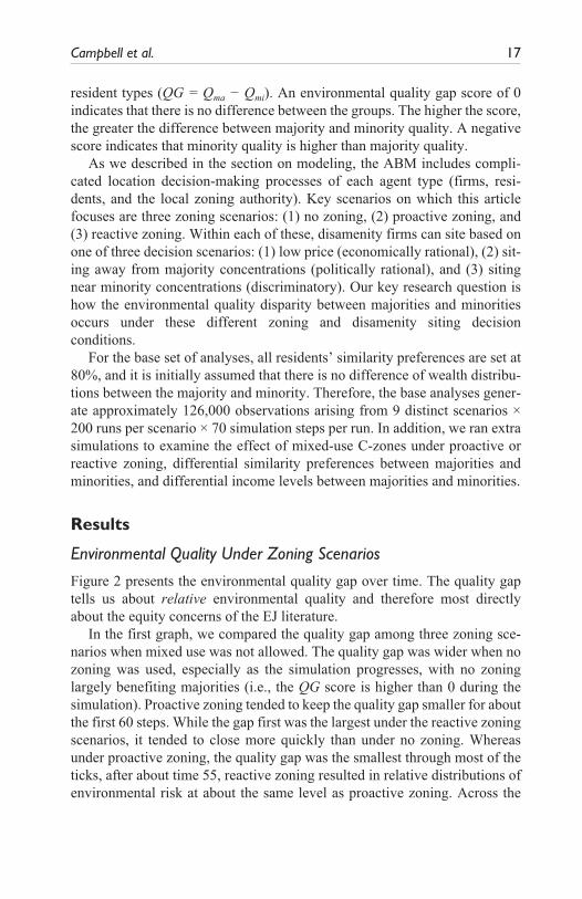
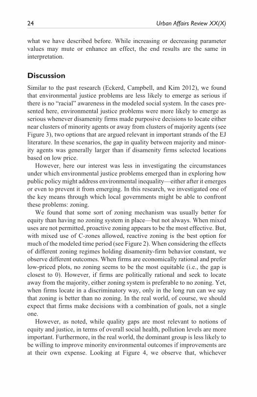
Environmental Quality Under Zoning ScenariosFigure 2 presents the environmental quality gap over time. The quality gap tells us about relative environmental quality and therefore most directly about the equity concerns of the EJ literature.

In the first graph, we compared the quality gap among three zoning sce-narios when mixed use was not allowed. The quality gap was wider when no zoning was used, especially as the simulation progresses, with no zoning largely benefiting majorities (i.e., the QG score is higher than 0 during the simulation). Proactive zoning tended to keep the quality gap smaller for about the first 60 steps. While the gap first was the largest under the reactive zoning scenarios, it tended to close more quickly than under no zoning. Whereas under proactive zoning, the quality gap was the smallest through most of the ticks, after about time 55, reactive zoning resulted in relative distributions of environmental risk at about the same level as proactive zoning. Across the

18

Figu

re 2

. Q

ualit

y ga

ps b

y zo

ning

str

ateg

ies.

Campbell et al. 19

scenarios, the size of the gap reaches its peak somewhere between times 40 and 50, depending upon the zoning mechanism, and begins to decline through the rest of the simulation. By time 70, the gap is about the same for both the proactive and reactive zoning scenarios. However, the quality gap remains larger under no-zoning scenarios. Therefore, in these scenarios, externality zoning, either proactive or reactive, lessens the environmental quality gap between the two social groups.

Figure 2 also compares the quality gap over time under proactive and reac-tive zoning combined with mixed use of C-zones. Here, residents are allowed to locate in C-zones in addition to unzoned areas. By time 20, the quality gap increases fastest—even faster than no-zoning—under proactive zoning with mixed use. After that, the quality gap is stabilized and remains at a level simi-lar to proactive zoning without mixed use. When reactive zoning is combined with mixed use, we found that the quality gap between majority and minority was the narrowest over time. At the end of the simulation, however, there is no significant difference in the quality gap between these two zoning sce-narios (which is also true in the scenarios without mixed use). The environ-mental quality gap under zoning scenarios is usually lower than that for no-zoning scenarios; the only exception is the case of proactive zoning with mixed use through about time 38.

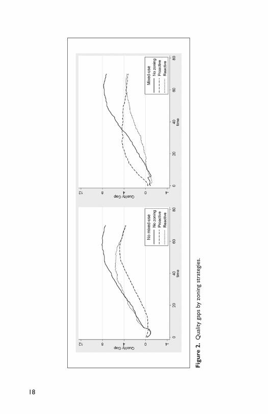
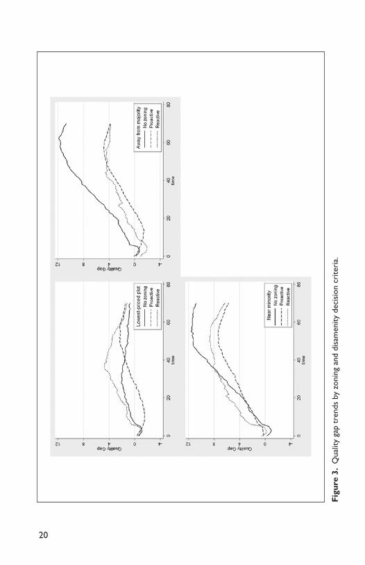
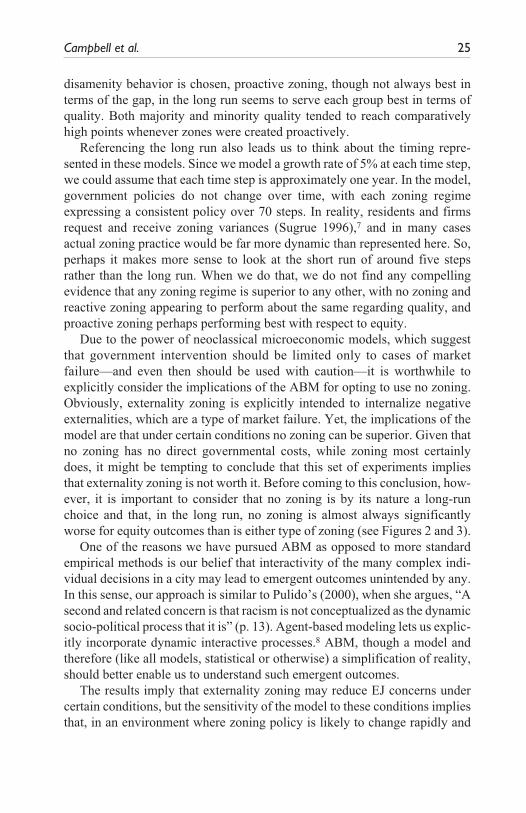
Aggregating all disamenity location scenarios together as in Figure 2 may miss important trends if, as some of the literature argues, different prefer-ences regarding disamenity location selection cause different outcomes. Figure 3 presents environmental quality gaps under the three different disa-menity location selection criteria described earlier. It includes all three base-line zoning scenarios (mixed use is not allowed). As can be seen in Figure 3, while an environmental quality gap does emerge whenever disamenities choose the lowest priced plots, the size of that gap is much smaller than when disamenities either avoid majority populations or site near minority popula-tions. The trend of the gap is similar over time if firms seek out locations near minority areas or if they simply avoid locating near majority populations, but the size of the quality gap is larger when disamenities site near minorities. In the case when disamenity firms seek to locate away from majorities, both proactive and reactive zoning reduce the quality gap significantly compared with the scenarios with no zoning. However, the situation is different when firms seek to locate near minorities; in these scenarios, zoning seems less efficacious as reactive zoning is actually worse than no zoning until about time 40, and proactive zoning is more effective than no zoning only after about time 20. In each of the cases, the gap opens during about the first 40 steps and then begins to decline later.

20

Figu

re 3

. Q

ualit

y ga

p tr

ends

by

zoni

ng a

nd d

isam

enity

dec

ision

cri

teri

a.

Campbell et al. 21

We should note that the size of the gap tells little about the trends in envi-ronmental quality for the two groups—a point that the EJ literature has tended to ignore. The gap can be closing in different ways. For example, majority quality can decrease or minority quality can increase (or both can occur simultaneously). Similarly, the gap can increase when both groups are expe-riencing increasing quality if majority quality increases at a higher rate. Yet, these different options have different implications for justice and health.

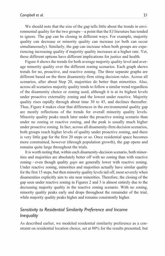
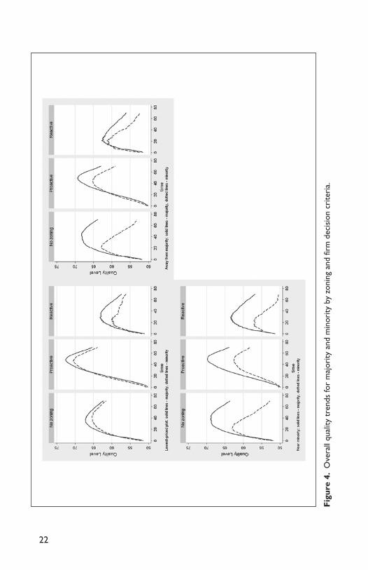
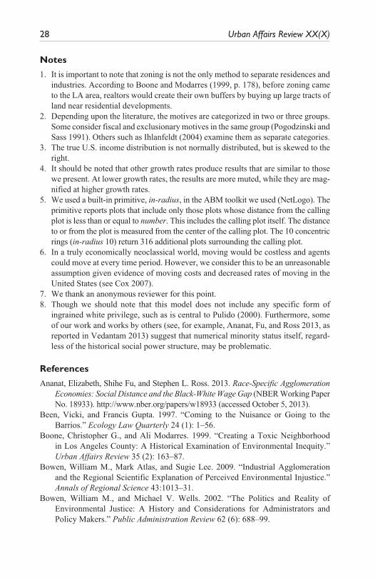
Figure 4 shows the trends for both average majority quality level and aver-age minority quality over the different zoning scenarios. Each graph shows trends for no, proactive, and reactive zoning. The three separate graphs are different based on the three disamenity-firm siting decision rules. Across all scenarios, after about Step 20, majorities do better than minorities. Also, across all scenarios majority quality tends to follow a similar trend regardless of the disamenity choice or zoning used, although it is at its highest levels under proactive externality zoning and the lowest under reactive. Majority quality rises rapidly through about time 30 to 45, and declines thereafter. Thus, Figure 4 makes clear that differences in the environmental quality gap are mostly reflections of the trends for overall minority quality levels. Minority quality peaks much later under the proactive zoning scenario than under no zoning or reactive zoning, and the peak is usually much higher under proactive zoning. In fact, across all disamenity-firm decision scenarios, both groups reach higher levels of quality under proactive zoning, and there is very little gap for the first 20 steps or so. Once residential space becomes more constrained, however (through population growth), the gap opens and remains quite large throughout the trials.

It is worth noting that, within each disamenity-decision scenario, both minor-ities and majorities are absolutely better off with no zoning than with reactive zoning—even though quality gaps are generally lower with reactive zoning. Under reactive zoning, minorities and majorities actually have similar quality for the first 15 steps, but then minority quality levels tail off, most severely when disamenities explicitly aim to site near minorities. Therefore, the closing of the gap seen under reactive zoning in Figures 2 and 3 is almost entirely due to the decreasing majority quality in the reactive zoning scenario. With no zoning, minority quality peaks early and drops throughout the remainder of the trial, while majority quality peaks higher and remains consistently higher.

Sensitivity to Residential Similarity Preference and Income InequalityAs described earlier, we modeled residential similarity preference as a con-straint on residential location choice, set at 80% for the results presented, but

22

Figu

re 4

. O

vera

ll qu

ality

tren

ds fo

r m

ajor

ity a

nd m

inor

ity b

y zo

ning

and

firm

dec

ision

cri

teri

a.

Campbell et al. 23

in testing the model we explored a host of different assumptions with respect to both the level of the similarity preference and the strength of the preference relative to other considerations. The results we present were consistent through most of these different scenarios, with some notable exceptions that could merit future consideration. When we altered similarity preferences, but kept both groups with the same level, say 50%, the results were similar to those presented earlier, if a bit more muted with this lower similarity prefer-ence. But when the two groups had different similarity preferences, the results were often quite different—most prominently with respect to the sce-narios where disamenity firms chose locations away from clusters of major-ity residents.

In a trial where majorities chose locations based on an 80% preference and minorities chose based on a 50% preference (a difference which is justified by some empirical work; see Clark 1992), minorities often saw higher aver-age quality levels than majorities. This result suggests that whenever firms have a preference for avoiding protracted political complications by siting away from higher status residents, and lower status residents are more apt to choose locations in higher status communities, the locations firms choose may end up being away from not just higher status residents, but also residen-tial settlement altogether.

Such outcomes could represent a potential best-case scenario; we need environmental disamenities to maintain economic growth and a high stan-dard of living, so disamenities must be located somewhere. While locating such facilities away from residential settlement may not be optimal in terms of the effect on the natural environment, it could be the ideal situation for achieving a relatively equitable distribution of environmental quality without making one group worse off.

Similarly, we ran trials with income equality and inequality (drawing on Census data for white non-Hispanics and African Americans, as discussed earlier). As would be expected, it was generally the case that the quality gap was smaller when there was income parity, but there are some significant caveats to this. In scenarios which included modeling of income inequality, the quality gap was relatively small when disamenities chose the lowest priced plot regardless of the zoning scenario, and it was larger when disame-nities chose either to locate away from the majority or near the minority. Interestingly, with income variability, and regardless of the scenario, the gap took longer to open than when there was income parity. This result may seem counterintuitive, but may simply be a reflection of the ample space for resi-dents to locate on during the initial phases of the simulation.

We ran similar sensitivity tests for virtually all of the other parameters in the model; in these tests we found results that were functionally the same as


what we have described before. While increasing or decreasing parameter values may mute or enhance an effect, the end results are the same in interpretation.

DiscussionSimilar to the past research (Eckerd, Campbell, and Kim 2012), we found that environmental justice problems are less likely to emerge as serious if there is no “racial” awareness in the modeled social system. In the cases pre-sented here, environmental justice problems were more likely to emerge as serious whenever disamenity firms made purposive decisions to locate either near clusters of minority agents or away from clusters of majority agents (see Figure 3), two options that are argued relevant in important strands of the EJ literature. In these scenarios, the gap in quality between majority and minor-ity agents was generally larger than if disamenity firms selected locations based on low price.

However, here our interest was less in investigating the circumstances under which environmental justice problems emerged than in exploring how public policy might address environmental inequality—either after it emerges or even to prevent it from emerging. In this research, we investigated one of the key means through which local governments might be able to confront these problems: zoning.

We found that some sort of zoning mechanism was usually better for equity than having no zoning system in place—but not always. When mixed uses are not permitted, proactive zoning appears to be the most effective. But, with mixed use of C-zones allowed, reactive zoning is the best option for much of the modeled time period (see Figure 2). When considering the effects of different zoning regimes holding disamenity-firm behavior constant, we observe different outcomes. When firms are economically rational and prefer low-priced plots, no zoning seems to be the most equitable (i.e., the gap is closest to 0). However, if firms are politically rational and seek to locate away from the majority, either zoning system is preferable to no zoning. Yet, when firms locate in a discriminatory way, only in the long run can we say that zoning is better than no zoning. In the real world, of course, we should expect that firms make decisions with a combination of goals, not a single one.

However, as noted, while quality gaps are most relevant to notions of equity and justice, in terms of overall social health, pollution levels are more important. Furthermore, in the real world, the dominant group is less likely to be willing to improve minority environmental outcomes if improvements are at their own expense. Looking at Figure 4, we observe that, whichever

Campbell et al. 25

disamenity behavior is chosen, proactive zoning, though not always best in terms of the gap, in the long run seems to serve each group best in terms of quality. Both majority and minority quality tended to reach comparatively high points whenever zones were created proactively.

Referencing the long run also leads us to think about the timing repre-sented in these models. Since we model a growth rate of 5% at each time step, we could assume that each time step is approximately one year. In the model, government policies do not change over time, with each zoning regime expressing a consistent policy over 70 steps. In reality, residents and firms request and receive zoning variances (Sugrue 1996),7 and in many cases actual zoning practice would be far more dynamic than represented here. So, perhaps it makes more sense to look at the short run of around five steps rather than the long run. When we do that, we do not find any compelling evidence that any zoning regime is superior to any other, with no zoning and reactive zoning appearing to perform about the same regarding quality, and proactive zoning perhaps performing best with respect to equity.

Due to the power of neoclassical microeconomic models, which suggest that government intervention should be limited only to cases of market failure—and even then should be used with caution—it is worthwhile to explicitly consider the implications of the ABM for opting to use no zoning. Obviously, externality zoning is explicitly intended to internalize negative externalities, which are a type of market failure. Yet, the implications of the model are that under certain conditions no zoning can be superior. Given that no zoning has no direct governmental costs, while zoning most certainly does, it might be tempting to conclude that this set of experiments implies that externality zoning is not worth it. Before coming to this conclusion, how-ever, it is important to consider that no zoning is by its nature a long-run choice and that, in the long run, no zoning is almost always significantly worse for equity outcomes than is either type of zoning (see Figures 2 and 3).

One of the reasons we have pursued ABM as opposed to more standard empirical methods is our belief that interactivity of the many complex indi-vidual decisions in a city may lead to emergent outcomes unintended by any. In this sense, our approach is similar to Pulido’s (2000), when she argues, “A second and related concern is that racism is not conceptualized as the dynamic socio-political process that it is” (p. 13). Agent-based modeling lets us explic-itly incorporate dynamic interactive processes.8 ABM, though a model and therefore (like all models, statistical or otherwise) a simplification of reality, should better enable us to understand such emergent outcomes.

The results imply that externality zoning may reduce EJ concerns under certain conditions, but the sensitivity of the model to these conditions implies that, in an environment where zoning policy is likely to change rapidly and


where not all actors will have externality zoning as the goal, it is unlikely to prove a consistently successful method of EJ improvement. This is disap-pointing because, as mentioned zoning is one of the policy options readily available to localities in the United States.

While these results should be taken with the appropriate amount of cau-tion, given our use of a simulation method, they do raise some interesting hypotheses that may be worth exploring further. Consider that, while most zoning systems across the United States share commonalities, there is much variation in how zoning is implemented and managed. Some states and local-ities have very flexible zoning rules, like much of the Sunbelt, while others have long-established zones that are less prone to alteration, like the spatially constrained Northeastern corridor cities. Others, like the aforementioned Houston and some other smaller cities, do not have zoning at all, and Houston has maintained its no-zoning regime over many decades. While additional contextual variables relating to these jurisdictions must also be taken into account, studying environmental justice outcomes comparatively across dif-ferent types of cities with different zoning systems could show interesting trends with respect to the relative equity of environmental quality; all else equal, our results suggest that land-use regulations may have different effects on EJ depending on how long they have been in place and how often they are varied—and their intents, of course.

ConclusionFor the most part, prior EJ research has focused on the question of whether minority-based environmental injustice exists. There seems to be sufficient evidence that it exists, at least sometimes, and so it is time to also consider questions regarding when it exists and what policy tools may ameliorate it. Through utilization of an agent-based simulation model, this article begins a process of shifting focus by examining a widely used tool of local govern-ment: zoning. The analysis indicates that the value of externality zoning is probably sensitive to other conditions such as how firms and residents make location choices as well as to the duration of the zoning regime. Furthermore, while the EJ literature focuses on quality gaps, overall levels of quality are also important, and the analysis has different implications for equity and for overall quality. In longer run scenarios, proactive zoning appears optimal for quality and any zoning is preferred to no zoning for equity. However, if cit-ies’ zoning regimes will be short-run and changeable, the value of externality zoning is much less clear.

This analysis also suggests some empirical analyses. For example, ceteris paribus, Houston should have worse environmental justice outcomes than

Campbell et al. 27

similar cities with a long, consistent externality-zoning regime. Newer cities that set up externality zoning proactively early in their development and hewed to it consistently should have smaller EJ gaps than similar-aged cities that zoned later. These are empirically testable hypotheses that can be used to validate the implications of the ABM presented here.

Taken all together, the findings of this simulation may suggest why some EJ studies find injustice while others do not: the simulation indicates that the extent of environmental injustice is a factor not only of firm decisions, but also of residential choices and local government policy. Taking a step back, it is not surprising that a broadly observed social trend has roots in the inter-action of decisions that individuals, organizations, and governments make. Nevertheless, EJ has largely been treated as a problem of firm or resident decision making, and policies to address the problem have largely flowed from the firm-behavior assumption (Bowen and Wells 2002). Our research suggests that successful policy response is unlikely to be “one size fits all,” but it must depend on contextual politics and culture that affect how the pol-icy tool is used.

Finally, this research more broadly identifies the potential strength of using simulation models to explore urban policy issues. The model and our results provide us with a new way to think about EJ, complementing existing analysis. Rather than investigating whether an unequal distribution of envi-ronmental quality exists, we explore conditions under which an unequal dis-tribution could be observed, and how one common tool of government policy could be utilized to address the problem. Furthermore, this model allows us to consider overall levels of environmental quality, rather than only the rela-tive levels, finding that some conditions lead to better quality for both groups. Although our model presents a simplified version of this tool of government policy, using ABM allows us to explore implications of utilizing zoning in a consequence-free environment that holds the potential to inform both the-ory—through the modeling of complex interactivity and the derivation of hypotheses—and practice, through the insight gained by experimenting with a common tool of government policy.

Declaration of Conflicting InterestsThe author(s) declared no potential conflicts of interest with respect to the research, authorship, and/or publication of this article.

FundingThe author(s) received no financial support for the research, authorship, and/or publi-cation of this article.


Notes1. It is important to note that zoning is not the only method to separate residences and

industries. According to Boone and Modarres (1999, p. 178), before zoning came to the LA area, realtors would create their own buffers by buying up large tracts of land near residential developments.

2. Depending upon the literature, the motives are categorized in two or three groups. Some consider fiscal and exclusionary motives in the same group (Pogodzinski and Sass 1991). Others such as Ihlanfeldt (2004) examine them as separate categories.

3. The true U.S. income distribution is not normally distributed, but is skewed to the right.

4. It should be noted that other growth rates produce results that are similar to those we present. At lower growth rates, the results are more muted, while they are mag-nified at higher growth rates.

5. We used a built-in primitive, in-radius, in the ABM toolkit we used (NetLogo). The primitive reports plots that include only those plots whose distance from the calling plot is less than or equal to number. This includes the calling plot itself. The distance to or from the plot is measured from the center of the calling plot. The 10 concentric rings (in-radius 10) return 316 additional plots surrounding the calling plot.

6. In a truly economically neoclassical world, moving would be costless and agents could move at every time period. However, we consider this to be an unreasonable assumption given evidence of moving costs and decreased rates of moving in the United States (see Cox 2007).

7. We thank an anonymous reviewer for this point.8. Though we should note that this model does not include any specific form of

ingrained white privilege, such as is central to Pulido (2000). Furthermore, some of our work and works by others (see, for example, Ananat, Fu, and Ross 2013, as reported in Vedantam 2013) suggest that numerical minority status itself, regard-less of the historical social power structure, may be problematic.

ReferencesAnanat, Elizabeth, Shihe Fu, and Stephen L. Ross. 2013. Race-Specific Agglomeration

Economies: Social Distance and the Black-White Wage Gap (NBER Working Paper No. 18933). http://www.nber.org/papers/w18933 (accessed October 5, 2013).

Been, Vicki, and Francis Gupta. 1997. “Coming to the Nuisance or Going to the Barrios.” Ecology Law Quarterly 24 (1): 1–56.

Boone, Christopher G., and Ali Modarres. 1999. “Creating a Toxic Neighborhood in Los Angeles County: A Historical Examination of Environmental Inequity.” Urban Affairs Review 35 (2): 163–87.

Bowen, William M., Mark Atlas, and Sugie Lee. 2009. “Industrial Agglomeration and the Regional Scientific Explanation of Perceived Environmental Injustice.” Annals of Regional Science 43:1013–31.

Bowen, William M., and Michael V. Wells. 2002. “The Politics and Reality of Environmental Justice: A History and Considerations for Administrators and Policy Makers.” Public Administration Review 62 (6): 688–99.

Campbell et al. 29

Brown, Daniel G., Scott Pages, Rick Riolo, Moria Zellner, and William Rand. 2005. “Path Dependence and the Validation of Agent–Based Spatial Models of Land.” Intenational Journal of Geographical Information Science 19:153–74.

Brown, Daniel G., and Derek T. Robinson. 2005. “Effects of Heterogeneity in Residential Preferences on an Agent-Based Model of Urban Sprawl.” Ecology and Society 11 (1): 46–66.

Bullard, Robert D. 1990. Dumping in Dixie: Race, Class, and Environmental Quality. Boulder: Westview Press.

Campbell, Heather E., Laura R. Peck, and Michael K. Tschudi. 2010. “Justice for All? A Cross-Time Analysis of Toxics Release Inventory Facility Location.” Review of Policy Research 27 (1): 1–25.

U.S. Census Bureau. 2010. Census, United States.[AQ: 1]Clark, Willam A. V. 1992. “Residential Preferences and Residential Choices in a

Multiethnic Context.” Demography 29 (3): 451–66.Cox, Kevin R. 2007. “Housing Tenure and Neighborhood Activism.” Urban Affairs

Review 18:107–29.Dear, Michael. 1992. “Understanding and Overcoming the NIMBY Syndrome.”

Journal of the American Planning Association 58 (3): 288–300.Desai, Anand. 2012. Simulations for Policy Inquiry. New York: Springer.Downey, Liam. 1998. “Environmental Injustice: Is Race or Income a Better Predictor.”

Social Science Quarterly 79 (4): 766–78.Eckerd, Adam, Heather E. Campbell, and Yushim Kim. 2012. “Helping Those Like

Us or Harming Those Unlike Us: Agent-Based Modeling to Illuminate Social Processes Leading to Environmental Injustice.” Environment and Planning B 39 (5): 945–64. doi:10.1068/b38001.

Epstein, Joshua M. 2006. Generative Social Science: Studies in Agent-Based Computational Modeling. Princeton: Princeton Univ. Press.

Fischel, William A. 1992. “Property Taxation and the Tiebout Model: Evidence for the Benefit View from Zoning and Voting.” Journal of Economic Literature 30 (1): 171–77.

Fischel, William A. 1997. The Economics of Zoning Laws: A Property Rights Approach to American Land Use Controls. Baltimore: Johns Hopkins Univ. Press.

Gilbert, Nigel. 2008. Agent-Based Models. Thousand Oaks, CA: Sage.Hamilton, James T. 1995. “Testing for Environmental Racism: Prejudice, Profits,

Political Power?” Journal of Policy Analysis and Management 14 (1): 107–32.Ihlanfeldt, Keith R. 2004. “Exclusionary Land-Use Regulations within Suburban

Communities: A Review of the Evidence and Policy Prescriptions.” Urban Studies 41 (2): 261–83.

Kraft, Michael E., and Bruce B. Clary. 1991. “Citizen Participation and the NIMBY Syndrome: Public Response to Radioactive Waste Disposal.” Political Research Quarterly 44:299–328.

Kriesel, Warren, Terence J. Centner, and Andrew G. Keeler. 1996. “Neighborhood Exposure to Toxic Releases: Are There Racial Inequities?” Growth and Change 27 (4): 479–99.


Krugman, Paul. 1993. “On the Relationship between Trade Theory and Location Theory.” Review of International Economics 1 (2): 110–22.

Lazero, Arthur S. 1971. “Discriminatory Zoning: Legal Battleground of the Seventies.” American University Law Review 21:157–83.

Ligmann-Zielinska, Arika, and Piotr Jankowski. 2010. “Exploring Normative Scenarios of Land Use Development Decisions with an Agent-Based Simulation Laboratory.” Computers, Environment and Urban Systems 34:409–23.

Maantay, Juliana. 2002. “Zoning Law, Health, and Environmental Justice: What’s the Conclusion?” Journal of Law, Medicine & Ethics 30:572–93.

McAvoy, Gregory E. 1998. “Partisan Probing and Democratic Decisionmaking: Rethinking the NIMBY Syndrome.” Policy Studies Journal 26 (2): 274–92.

Noonan, Douglas S. 2008. “Evidence of Environmental Justice: A Critical Perspective on the Practice of EJ Research and Lessons for Policy Design.” Social Science Quarterly 89 (5): 1153–74.

Ohls, James C., Richard Chadbourn Weisberg, and Michelle J. White. 1974. “The Effect of Zoning on Land Value.” Journal of Urban Economics 1 (4): 428–44.

Parker, Dawn C., and Tatiana Filatova. 2008. “A Conceptual Design for a Bilateral Agent-Based Land Market with Heterogeneous Economic Agents.” Computers, Environment and Urban Systems 32 (6): 454–63.

Parker, Dawn C., Steven M. Manson, Marco A. Janssen, Matthew J. Hoffmann, and Peter Deadman. 2003. “Multi-agent Systems for the Simulation of Land-Use and Land-Cover Change: A Review.” Annals of the Association of American Geographers 93 (2): 314–37.

Parker, Dawn C., and Vicky J. Meretsky. 2004. “Measuring Pattern Outcomes in an Agent-Based Model of Edge-Effect Externalities Using Spatial Metrics.” Agriculture Ecosystem & Environment 101:233–50.

Pastor, Manuel, Rachel Morello-Frosch, and James L. Sadd. 2005. “The Air Is Always Cleaner on the Other Side: Race, Space, and Ambient Air Toxics Exposures in California.” Journal of Urban Affairs 27 (2): 127–48.

Pastor, Manuel, Jim Sadd, and John Hipp. 2001. “Which Came First? Toxic Facilities, Minority Move-In, and Environmental Justice.” Journal of Urban Affairs 23 (1): 1–21.

Pendall, Rolf. 2000. “Local Land Use Regulation and the Chain of Exclusion.” Journal of the American Planning Association 66 (2): 125–42.

Pogodzinski, J. Mike, and Tim R. Sass. 1991. “Measuring the Effects of Municipal Zoning Regulations: A Survey.” Urban Studies 28 (4): 591–621.

Pratt, John W. 1964. “Risk Aversion in the Small and the Large.” Econometrica 32 (1–2): 122–36.

Pulido, Laura. 2000. “Rethinking Environmental Racism: White Privilege and Urban Development in Southern California.” Annals of the Association of American Geographers 90 (1): 12–40.

Qian, Zou. 2011. “Shaping Urban Form without Zoning: Investigating Three Neighborhoods in Huston.” Planning Practice & Research 261 (1): 21–42.

Campbell et al. 31

Rand, William, Moira Zellner, Scott E. Page, Rick Riolo, Daniel G. Brown, and L. E. Fernandez. 2002. “The Complex Interaction of Agents and Environments: An Example in Urban Sprawl.” In Proceedings of the Agent 2002 Conference on Social Agents: Ecology, Exchange and Evolution, edited by Charles Macal, and David Sallach, 149–61. Chicago: University of Chicago and Argonne National Lab.

Richardson, Harry W., Peter Gordon, M. J. Jun, and M. H. Kimm. 1993. “Pride and Prejudice: The Economic Impacts of Growth Controls in Pasadena.” Environment & Planning 25 (7): 987–1002.

Ringquist, Evan J. 2005. “Assessing Evidence of Environmental Inequities: A Meta-analysis.” Journal of Policy Analysis and Management 24 (2): 223–47.

Rothwell, Jonathan, and Douglas S. Massey. 2009. “The Effect of Density Zoning on Racial Segregation in U.S. Urban Areas.” Urban Affairs Review 44 (6): 779–806.

Saha, Robin, and Paul Mohai. 2005. “Historical Context and Hazardous Waste Facility Siting.” Social Problems 52 (4): 618–48.

Schelling, Thomas C. 1971. Micromotives and Macrobehavior. New York: Norton.Schilling, Joseph, and Leslie S. Linton. 2005. “The Public Health Roots of Zoning in

Search of Active Living’s Legal Genealogy.” American Journal of Preventive Medicine 28 (2, Suppl. 2): 96–104.

Sugrue, Thomas J. 1996. The Origins of the Urban Crisis: Race and Inequality in Postwar Detroit. Princeton: Princeton Univ. Press.

Tesfatsion, Leigh, and Kenneth L. Judd. 2006. Handbook of Computational Economics: Agent-Based Computational Economics? Oxford: Elsevier.[AQ: 2]

Tobler, Waldo R. 1970. “A Computer Movie Simulating Urban Growth in the Detroit Region.” Economic Geography 46 (2): 234–40.

Torrens, Paul M., and Atsushi Nara. 2007. “Modeling Gentrification Dynamics: A Hybrid Approach.” Computers, Environment and Urban Systems 31:337–61.

Vedantam, Shankar. 2013. “Being in the Minority Can Cost You and Your Company.” http://www.npr.org/blogs/codeswitch/2013/07/24/204898755/wage-gap-research (accessed October 5, 2013).

Veldkamp, A., and P. Verburg. 2004. “Modeling Land Use Change and Environmental Impact.” Journal of Environmental Management 72:1–3.

Wilson, Sacoby, Malo Hutson, and Mahasin S. Mujahid. 2008. “How Planning and Zoning Contribute to Inequitable Development, Neighborhood Health, and Environmental Injustice.” Environmental Justice 1 (4): 211–16.

Wolverton, Ann. 2009. “Effects of Socio-economic and Input-Related Factors on Polluting Plants’ Location Decisions.” B.E. Journal of Economic Analysis & Policy 9 (1): 1–32.

Woodworth, James R., W. Robert Gump, and James R. Forrester. 2006. Camelot: A Role Playing Simulation of Political Decision Making. Belmont: Thompson.

Zellner, Moira L., Scott E. Page, William Rand, Daniel G. Brown, Derek T. Robinson, Joan Nassauerd, and Bobbi Lowd. 2009. “The Emergence of Zoning Policy Games in Exurban Jurisdictions: Informing Collective Action Theory.” Land Use Policy 26:356–67.


Zellner, Moira L., Rick L. Riolo, William Rand, Daniel G. Brown, Scott E. Page, and Luis E. Fernandez. 2010. “The Problem with Zoning: Nonlinear Effects of Interaction between Location Preferences and Externalities on Land Use and Utility.” Environment and Planning B 37:408–28.

Author BiographiesHeather E. Campbell is a professor and chair of the Department of Politics and Policy and Department of Economics at the Claremont Graduate University, School of Social Science, Policy and Evaluation. She is the coauthor of Urban Environmental Policy Analysis (2012). Her current research focuses on environmental policy, and particularly on environmental justice. She has served as the editor of the Journal of Public Affairs Education.

Yushim Kim is an associate professor at the School of Public Affairs at the Arizona State University. She specializes in policy analysis and policy informatics, and her research interests focus on issues in public service provision and management. She has published refereed articles on public health and welfare policy as well as on spa-tial and agent-based modeling.

Adam Eckerd is an assistant professor with the Center for Public Administration and Policy in the School of Public and International Affairs at Virginia Tech. He conducts research on the complex relationship between government decisions and social out-comes, particularly with respect to environmental justice, public participation, and nonprofit organizations.