


Bahasa
Halaman
Hukum

WISSENSCHAFTSZENTRUM BERLINFÜR SOZIALFORSCHUNG
discussion papersSOCIAL SCIENCE RESEARCHCENTER BERLIN
FS IV 98 - 13
Learning in Sender-Receiver Games
Andreas BlumeDouglas V. DeJongGeorge R. NeumannNathan E. Savin
University of Iowa
September 1998
ISSN Nr. 0722 - 6748
ForschungsschwerpunktMarktprozeß und Unter-nehmensentwicklung
Research AreaMarket Processes andCorporate Development

Zitierweise/Citation:
Andreas Blume, Douglas V. DeJong, George R. Neumann, Nathan E.Savin, Learning in Sender-Receiver Games, Discussion PaperFS IV 98 - 13, Wissenschaftszentrum Berlin, 1998.
Wissenschaftszentrum Berlin für Sozialforschung gGmbH,Reichpietschufer 50, 10785 Berlin, Tel. (030) 2 54 91 - 0
ABSTRACT
Learning in Sender-Receiver Games
by Andreas Blume, Douglas V. DeJong, George R. Neumann and Nathan E. Savin*
Stimulus-response (SR) and belief-based learning (BBL) models are estimated withexperimental data from sender-receiver games and compared using the Davidson andMacKinnon P-test for non-nested hypotheses. Depending on a certain adjustmentparameter, the P-test favors the SR model, the BBL model or neither of the models.Following Camerer and Ho, the models are also compared to a hybrid model thatincorporates a mixture of both types of learning. The hybrid model is frequently notsignificantly better than either the SR or the BBL model. The sensitivity of the results toobservations taken after learning has ceased is investigated.
ZUSAMMENFASSUNG
Lernen in Sender-Empfänger-Spielen
Reiz-Reaktions- und überzeugungsgestützte Lernmodelle werden anhand von experi-mentellen Daten eines Senders-Empfänger-Spiels geschätzt und anhand des Davidsonund MacKinnon P-Tests für nicht eingebundene Hypothesen verglichen. In Abhängigkeiteines bestimmten Anpassungsparameters stützt der P-Test das Reiz-Reaktions-Modell,das überzeugungsgestützte Lernmodell bzw. keines der Modelle. In Anlehnung anCamerer und Ho werden die Modelle auch in Form eines hybriden Modells verglichen,das eine Mischung beider Typen des Lernens beinhaltet. Das Hybridmodell ist häufignicht signifikant besser als das Reiz-Reaktions-Modell bzw. das überzeugungsgestützteLernmodell. Außerdem wird die Sensitivität der Ergebnisse im Hinblick auf Beobach-tungen aufgezeigt, die nach Abschluß des Lernens gemacht wurden.
* We gratefully acknowledge the helpful comments of Drew Fudenberg in early discussions and
Al Roth and Ido Erev for giving us access to their software.
LEARNING IN SENDER-RECEIVER GAMES
In this paper, we investigate the strengths and weaknesses of cognitively simple
adaptive learning models. We do this by using experimental data that challenge these
models. The data is from sender-receiver games, games that play a prominent role in
theory and applied work in accounting, economics, finance and political science. For
example, see David Austen-Smith (1990), Vincent P. Crawford and Joel Sobel (1982),
Joseph Farrell and Robert Gibbons (1990), Frank Gigler (1994) and Jeremy Stein (1989).
The most striking fact from our analysis is that these simple learning models fit the data
remarkably well. We have compared the models using various statistical techniques and
have found it difficult to distinguish between the models. In the face of this difficulty, we
propose an agenda for future research on learning in games.
We use experimental data to investigate how much available information players use
when learning how to play a game. Three appealing criteria for a learning model are the
following: (1) learning at the level of the individual; (2) stochastic choice; and (3)
parsimony. One well-known model which satisfies all three of these criteria, besides
being consistent with some of the stylized facts established in the psychological learning
literature, is the stimulus-response SR model of Alvin Roth and Ido Erev (1995).
Furthermore, SR learning requires only minimal cognitive abilities on the part of players.
This feature of the model is appealing for those who want to show that high-rationality
predictions can be derived from a low-rationality model. A closely related feature is that
SR learning requires only minimal information. All that players need to know are the
payoffs from their own past actions; they need not know that they are playing a game,
they need not know their opponents’ payoff or their past play. These two closely related
features make the SR model a natural benchmark in our investigation. In addition, it can
be applied in a wide variety of settings.
On the other hand, it seems quite likely that individuals would try to exercise more
cognitive ability and hence try to use other available information. In belief based learning
(BBL) models, like fictitious play (Julia Robinson, 1951) or one of its stochastic variants
(Drew Fudenberg and David M. Kreps, 1993), the players use more information than

2
their own historical payoffs. This information may include their own opponents’ play, the
play of all possible opponents and the play of all players. Models of this kind embody a
higher level of rationality; e.g. fictitious play can be interpreted as optimizing behavior
given beliefs that are derived from Bayesian updating.
In this paper, we compare a simple BBL model against the SR model using
experimental data from extensive form games (Andreas Blume, Douglas V. DeJong,
Yong-Gwan Kim and Geoffrey B. Sprinkle (1998)). The players are members of a
population of players, senders and receivers. The population environment mitigates
repeated game effects and, therefore, is particularly suitable for evaluating myopic
learning rules. The players learn only about actions, not strategies of other players, either
privately or at the population level. When population information is available, it is only
about sender play. In this environment, learning is essential for players to coordinate
because messages are costless and a priori meaningless. The environment is challenging
for the learning models because in formulating the SR model for this extensive form
setting we have to decide whether the players are updating actions or strategies. We
choose actions on the grounds that this is cognitively simpler than strategies. For BBL it
is challenging because senders do not have direct information on receiver behavior at the
population level. For all treatments, we ask whether the SR model or the BBL model
better describes learning. The initial step in our analysis was to fit the SR and BBL
models to the data produced by the various treatments. We found that, regardless of
treatment, both models fit about equally well as measured by the coefficient of
determination.
We let the BBL model take a form that is analogous to the SR model. In both cases
choice probabilities depend on unobserved propensities. The models differ in how the
propensities are updated. In the SR model the propensity for taking an action is solely
dependent on a player’s own past payoffs from that action, whereas in the BBL model
the propensity depends on the average payoff across all players who took that action.
One way to calculate the unobserved propensities is to impose the parameter values used
in the literature. We found, however, that these values are overwhelmingly rejected by
data. Clearly, the SR and BBL models are non-nested because they employ different

3
information variables. For the purpose of comparing non-nested models, the natural
approach is to use a non-nested testing procedure. In this paper, we employ the Russell
Davidson and James G. MacKinnon (1984, 1993) P-test for non-nested hypotheses. The
outcome of the P-test is sensitive to the value chosen for the adjustment parameter.
When comparing the SR versus the BBL model, we show that depending on the value
selected for the adjustment parameter, the P-test favors the SR model, the BBL model or
neither of these models.
Colin Camerer and Teck-Hua Ho (1997) recognized that SR and BBL models are
nested in a general class of models which use propensities to determine choice
probabilities. Their approach is adapted to our setting, taking into account that in our
data players observe actions and not strategies and have information on an entire
population of players. In the more general model we employ, the propensities are
updated using both own and population average payoffs, and hence it is, intuitively
speaking, a hybrid of the SR and BBL models. We compared the SR and BBL models to
the hybrid model using likelihood ratio tests. The hybrid model was frequently not
significantly better than either the SR or the BBL model.1
A point often overlooked in empirical work is that information about learning can
only come from observations where learning occurs. Once behavior has converged,
observations have no further information about learning. Including such observations
will make the SR and BBL models appear to fit better, while at the same time reducing
the contrast between the models, making it difficult to distinguish the models empirically.
We call this effect convergence bias. A preliminary examination suggested that our non-
nested results were affected to some degree by convergence bias. Accordingly, we
eliminated observations where it appeared that learning has ceased and reanalyzed the
remaining data. The results of this reexamination were not markedly different from our
1 The nature of BBL in our paper is affected by the fact that players play extensive form games and
do so as members of a population of players. In Camerer and Ho (1997) strategies are„hypothetically reinforced“ based on the payoff the strategies would have yielded, irrespective ofwhether they were used. In our setting, this hypothetical reinforcement is more difficult becauseplayers learn only about the consequences of their actions and not what their opponent would havedone in response to a different action. On the other hand, our players can learn from theexperience of other players, in particular, from population history.
4
original finding. The convergence effect can strongly influence the results using the
hybrid model because it induces collinearity between the two information variables.
Recognizing the difficulty of discriminating among the various learning models, the last
section of the paper outlines an agenda for how we can learn more about learning in
games.
I. GAMES AND EXPERIMENTAL DESIGN
Our data are generated from repeated play of sender-receiver games among
randomly matched players. Players are drawn from two populations, senders and
receivers, and rematched after each round of play. The games played in each round are
between an informed sender and an uninformed receiver. The sender is privately
informed about his type, t1 or t2, and types are equally likely. The sender sends a
message, * or #, to the receiver, who responds with an action, a1, a2 or a3. Payoffs
depend on the sender's private information, his type, and the receiver's action, and not on
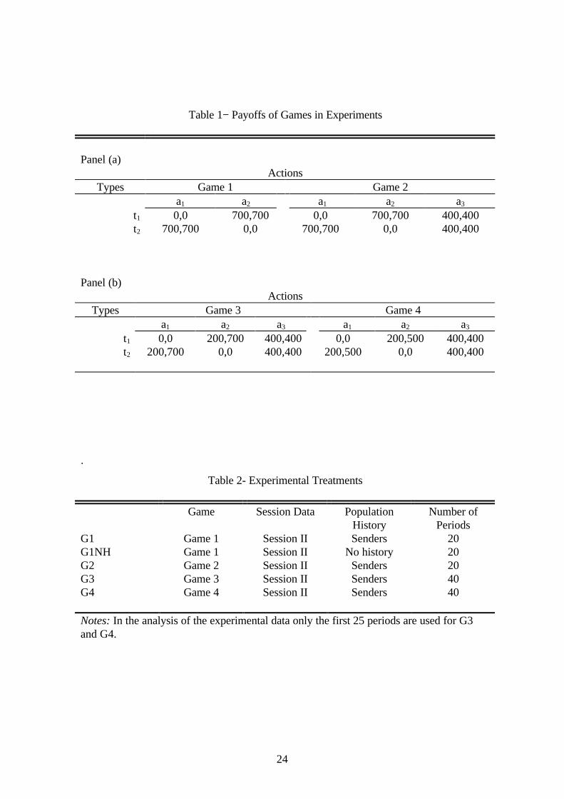
the sender’s message. The payoffs used in the different treatments are given in Table 1
below, with the first entry in each cell denoting the sender’s payoff and the second entry
the receiver’s payoff. For example, in Game 2, if the sender's type is t1 and the receiver
takes action a2, the payoffs to the sender and receiver are 700,700, respectively.
A strategy for the sender maps types into messages; for the receiver, a strategy maps
messages to actions. A strategy pair is a Nash equilibrium if the strategies are mutual
best replies. The equilibrium is called separating if each sender type is identified through
his message. In a pooling equilibrium, the equilibrium action does not depend on the
sender's type; such equilibrium exists for all sender-receiver games. In Game 2, an
example of a separating equilibrium is one where the sender sends * if he is t1 and #
otherwise and the receiver takes action a2 after message * and a1 otherwise. An example
of a pooling equilibrium is one in which the sender, regardless of type, sends * and the
receiver always takes action a3.

5
A replication of a game is played with a cohort of twelve players, six senders and six
receivers. Players are randomly designated as either a sender or receiver at the start of
the replication and keep their designation throughout. In each period of a game, senders
and receivers are paired using a random matching procedure. Sender types are
independently and identically drawn in each period for each sender.
In each period, players then play a two-stage game. Prior to the first stage, senders
are informed about their respective types. In the first stage, senders send a message to
the receiver they are paired with. In the second stage, receivers take an action after
receiving a message from the sender they are paired with. Each sender and receiver pair
then learns the sender type, message sent, action taken and payoff received. All players
next receive information about all sender types and all messages sent by the respective
sender types. This information is displayed for the current and all previous periods of the
replication.
To ensure that messages have no a priori meaning, each player is endowed with his
own representation of the message space, i.e. both the form that messages take and the
order in which they are represented on the screen is individualized. The message space
M = {*, # } is observed by all players and for each player either appears in the order #,*
or *, #. Unique to each player, these messages are then mapped into an underlying,
unobservable message space, M = {A,B}. The mappings are designed such that they
destroy all conceivable focal points that players might use for a priori coordination,
Blume et al. (1998). The representation and ordering are stable over the replication.
Thus, the experimental design focuses on the cohort's ability to develop a language as a
function of the game being played and the population history provided.
Note that in this setting we learn the players’ action choices, not their strategies.
Also, the players themselves receive information about actions, not strategies. They do
not observe which message (action) would have been sent (taken) by a sender (receiver)
had the sender's type (message received) been different. This is important for how we
formulate our learning rules; e.g. in our setting the hypothetical updating (see Camerer
and Ho (1997)) of unused actions that occurs in BBL cannot rely on knowing
opponents’ strategies but instead uses information about the population distribution of

6
play. For example, for the receiver the best reply to a message that he did not receive is
determined by the distribution of sender types that sent the messages.
We consider five experimental treatments, each with three replications. Each
replication is divided into two sessions, Session I, which is common to all treatments and
Session II, which varies across treatments. We concentrate on Session II data. In each
treatment, there are two populations of players, senders and receivers, where in each
round one sender is randomly matched with one receiver to play a given sender-receiver
game. The treatments examined here differ in terms of the players’ incentives and the
information that is available after each round of play. For one treatment, the only
information available to a player is the history of play in her own past matches. Two
questions are examined for these cases. The first is whether learning takes place. If
learning does take place, the second question is whether learning is captured by the SR
model. In all the other treatments, there is information available to the players in addition
to the history of play in their own past matches. For both senders and receivers, this
information is the history of play of the population of senders. Three questions are
examined for these treatments. The first again is whether learning takes place. If learning
does take place, the second question is whether learning is different from that in the
previous treatment, and the third is whether the BBL model better describes learning
than the SR model.
The data from the experiments in Blume et al. (1998) consists of three replications
for each game. Replications for Game 1 and 2 were played for 20 periods and Game 3
and 4 for 40 periods.2 There were two different treatments conducted with Game 1, one
with and one without population history. The treatments are summarized in Table 2.
In this paper we focus on the analysis of sender behavior using the data from the
second session. The attraction of concentrating on sender behavior is that senders have
the same number of strategies in all of our treatments. A potential drawback of this focus
2 All replications had a common session, which preceded the games described above. In particular,
each cohort participated in 20 periods of a game with payoffs as in Game 1 and a message space ofM = {A,B}. The common session provides players with experience about experimental proceduresand ensures that players understand the structure of the game, message space and populationhistory.

7
is that since senders do not receive information about the history of receiver play at the
population level, they cannot form beliefs based on that information. Instead they have to
make inferences from what they learn about sender population. We also examined
receiver behavior and found essentially the same results as for senders.
II. TESTING SR AND BBL MODELS
In this section we report the results of estimation of SR and BBL models of
behavior. The models are similar in that both use propensities to determine choice
probabilities. In our extensive form game setting, we have to make a choice of whether
we want to think of players as updating propensities of actions or of strategies. Both
choices constrain the way in which the updating at one information set affects the
updating at other information sets. If actions are updated, then there are no links across
information sets. If strategies are updated, then choice probabilities change continually at
every information set. We chose updating of actions, which amounts to treating each
player-information set pair as a separate player. We use the index i to refer to such a pair
(n, θ), where n denotes one of the six senders, θ a type realization for that sender, and
the pair i is called a player.
By SR we mean that individual play is affected only by rewards obtained from own
past play. Specifically, following Alvin E. Roth and Ido Erev (1995) define the
propensity, Qij(t), of player i to play action j at time t as:
(1) Q t Q t X tij ij ij( ) ( ) ( )= − + −ϕ ϕ0 11 1
where Xij(t-1) is the reward player i receives from taking action j at time t-1. Time here
measures the number of occurrences of a specific type for a fixed sender and ϕ0 measures
the lag effect (i.e. the importance of forgetting). Note that t is not real time. Given this
specification of propensities, the probability that player i takes action j is a logit function3
3 The specification of the logit function in (2) exploits the fact that all rewards, X, in the games that

8
(2) P t Player i takes action j at time tQ t
Q tijij
ijj
( ) Pr( )( )
( ).= =
′′
∑
To complete the specification of the SR model we require an initial condition for the
propensities- the values of Qij(1). Values chosen for Qij(1) affect Pij(1) and the speed
with which rewards change probabilities of playing a particular action. In the spirit of
Roth and Erev (1995) we set Qi1(1) = Qi2(1) = 350, which is on the scale of rewards
received by participants in the experiments.
For these experiments we examine the behavior of senders, who can be of two types.
Each type could send message „1“ or „2“. Let y = I{message = „2“}, where I{A} is the
indicator function that takes the value 1 if event A occurs and 0 otherwise. The log
likelihood function for the sender data is
(3) ln ( , ) ( ) ln( ( )) ( ( )) ln( ( )).l y t P t y t P ti i it
T
i
N
iϕ ϕ0 1 221
21 1= + − −==∑∑
The likelihood function was maximized separately for each of the 15 replications
using observations from round 2 onwards. Because the quantal choice model has a
regression structure the maximization can be achieved by Iteratively Re-Weighted Least
Squares. The results of doing so are shown in Table 3. Columns 2 and 3 of the table
contain the maximum likelihood (ML) estimates of ϕ0 and ϕ1 and columns 4 and 5
contain the log likelihood value at the optimum, and McFadden's (1974) psuedo-R2
statistic, defined as 1- ln(L)U/ln(L)R, where LR is the restricted value of the likelihood
function and LU is the unrestricted value. Here we take the restricted value as L= (p2)N.
Column 6 contains the likelihood ratio test statistic for testing the hypothesis H0:
ϕ0 = 1.0, which is the value proposed and used by Roth and Erev in their simulations.
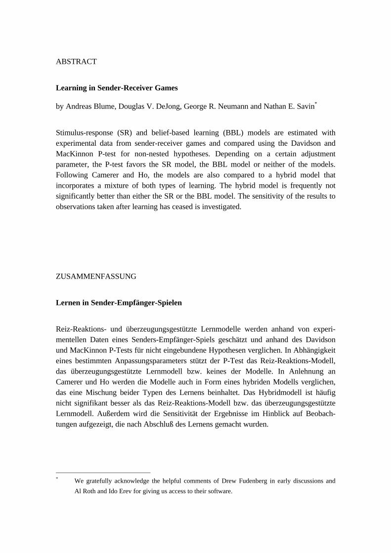
Two features stand out in the table. First, estimates of ϕ0 are generally quite far
from 1, judging from the LR test p-values reported in column 7.. Second, the SR model,
we examine are non-negative. Were this not the case, a transform that keeps the value of thepayoffs non-negative, such as the exponential function, can be used.
9
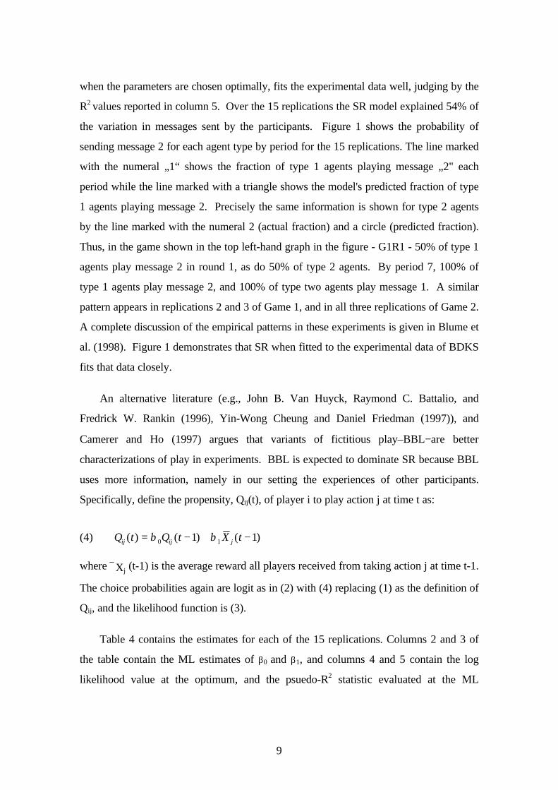
when the parameters are chosen optimally, fits the experimental data well, judging by the
R2 values reported in column 5. Over the 15 replications the SR model explained 54% of
the variation in messages sent by the participants. Figure 1 shows the probability of
sending message 2 for each agent type by period for the 15 replications. The line marked
with the numeral „1“ shows the fraction of type 1 agents playing message „2" each
period while the line marked with a triangle shows the model's predicted fraction of type
1 agents playing message 2. Precisely the same information is shown for type 2 agents
by the line marked with the numeral 2 (actual fraction) and a circle (predicted fraction).
Thus, in the game shown in the top left-hand graph in the figure - G1R1 - 50% of type 1
agents play message 2 in round 1, as do 50% of type 2 agents. By period 7, 100% of
type 1 agents play message 2, and 100% of type two agents play message 1. A similar
pattern appears in replications 2 and 3 of Game 1, and in all three replications of Game 2.
A complete discussion of the empirical patterns in these experiments is given in Blume et
al. (1998). Figure 1 demonstrates that SR when fitted to the experimental data of BDKS
fits that data closely.
An alternative literature (e.g., John B. Van Huyck, Raymond C. Battalio, and
Fredrick W. Rankin (1996), Yin-Wong Cheung and Daniel Friedman (1997)), and
Camerer and Ho (1997) argues that variants of fictitious play–BBL−are better
characterizations of play in experiments. BBL is expected to dominate SR because BBL
uses more information, namely in our setting the experiences of other participants.
Specifically, define the propensity, Qij(t), of player i to play action j at time t as:
(4) Q t Q t X tij ij j( ) ( ) ( )= − + −β β0 11 1
where Xj (t-1) is the average reward all players received from taking action j at time t-1.
The choice probabilities again are logit as in (2) with (4) replacing (1) as the definition of
Qij, and the likelihood function is (3).
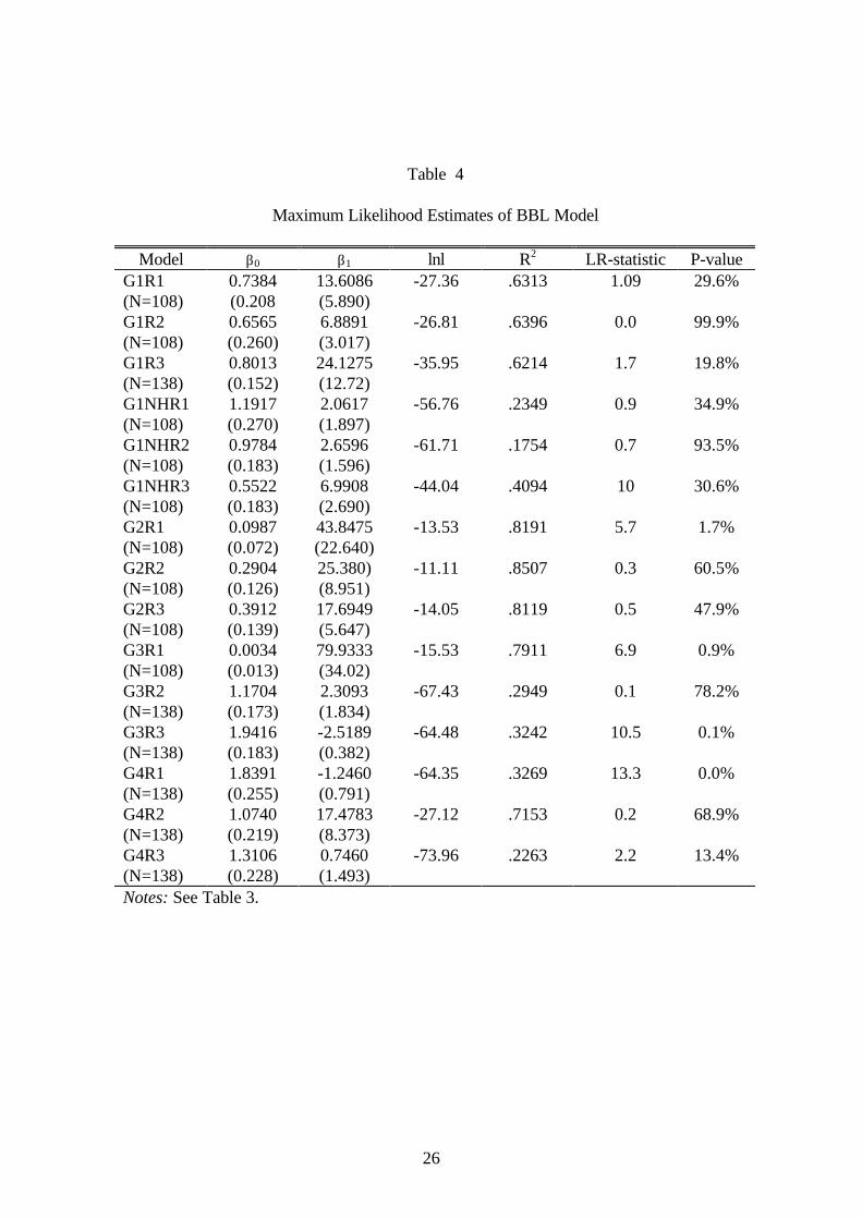
Table 4 contains the estimates for each of the 15 replications. Columns 2 and 3 of
the table contain the ML estimates of β0 and β1, and columns 4 and 5 contain the log
likelihood value at the optimum, and the psuedo-R2 statistic evaluated at the ML

10
estimates. Column 6 contains the likelihood ratio test statistic for the hypothesis H0:β0 =
1.
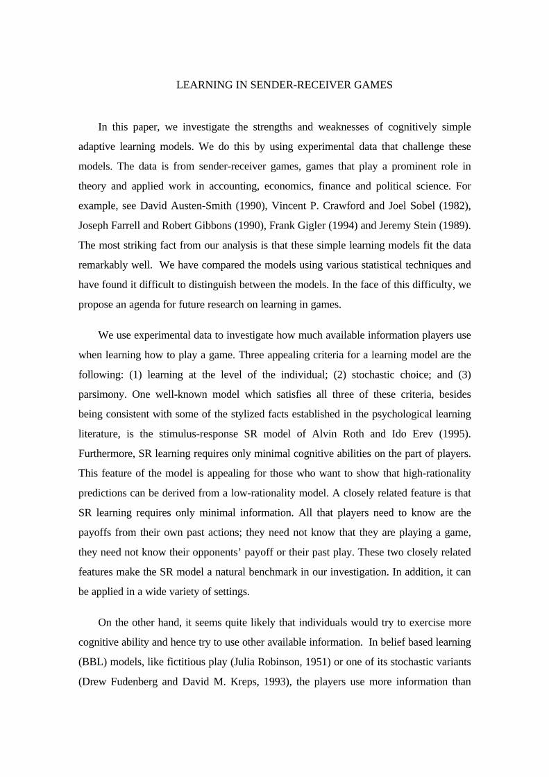
Again, two features stand out in the table. First, the estimates of β0 are generally
fairly close to 1. Second, the BBL model, when the parameters are chosen to maximize a
likelihood function, also fits the experimental data well. In the 15 cases the R2 value
ranges from .62 to .97; on average the BBL model explains 52% of the variation in
messages sent. The fit of this model is illustrated in Figure 2, which shows the relation
of predicted response and actual response by period. The comparison of R2’s is
suggestive: BBL „wins“ in most cases with population history information, SR wins
without that information.
On a technical note, the likelihood ratio test that H0: ϕ0 = 1 is invariant to the value
of the initial condition and similarly for the test that H0: β0 = 1. The initial condition
determines the values of ϕ1 and β1, but does not influence the values of ϕ0 and β0 .
III. COMPARING SR AND BBL MODELS
Figures 1 and 2 demonstrate the problem of distinguishing SR and BBL models of
behavior. Both SR and BBL learning fit the data well; hence, distinguishing these
models is difficult. For example, in the BDKS data the average difference in R2 is .02,
and the typical sample size is 108. Thus, an eyeball test does not show a great
preference for one learning specification. But an eyeball test may not be very powerful in
these circumstances so resort might be had to a more formal testing procedure. Making
probabilistic comparisons between the SR and BBL models is difficult because the
models are non-nested. By a nested model we mean that the model being tested, the null
hypothesis, is simply a special case of the alternative model to which it is compared. We
compare the SR and BBL models in a non-nested framework. In particular, we employ
Davidson and MacKinnon’s P-test for non-nested hypothesis testing in the following
manner. Write the models described in equations (1) and (4) and a nested composite
model as:
11
(5)
H E y t F Q t X t
H E y t F Q t X t
H E y t F Q t X t F Q t X t
i ij ij
i ij j
c i ij ij ij j
1 1
2 2
1 2
1 1
1 1
1 1 1 1 1
: ( ( )) ( $ ( ), ( ); )
: ( ( )) (~
( ), ( ); )
: ( ( )) ( ) ( $ ( ), ( ), ) (~
( ), ( ); )
= − −= − −
= − − − + − −
ϕβ
α ϕ α β
where ϕ and β are (k+1) x 1 dimension vectors with k the dimensionality of Xij , and
$Qij and ~Qij are the propensities evaluated at the estimated parameter values. Models 1
and 2 differ because Xij ≠ Xj, and hence the Q’s differ. (The Q’s differ when the
information variables are the same if ϕ 0 and β 0 differ.) To reinforce the latter point, the
two Q’s are distinguished by using a hat and a tilde. Following Davidson and MacKinnon
(1984, 1993) we test H1 against HC by estimating α in the artificial regression
(6) $ ( $ ) $ $ $ ( $ $ )/ / /V y F V f X V F F residualij− − −− = + − +1 2
11 2
1 01 2
2 1ϕ α
where V-1/2 is the square root of the variance covariance matrix for the dichotomous
variable y. For this purpose, ϕ 0 can be set equal to ϕ SR, β BBL, or estimated in
conjunction with α. In the same fashion we test H2 against HC by constructing a similar
artificial regression where β 0 can be set equal to ϕ SR, β BBL or estimated in conjunction
with α. The test for nesting is a test of the hypothesis that α = 0. There are four
outcomes that can arise from this pair of tests: (a) accept both models; (b) reject both
models; (c) accept model 1 and reject model 2; and (d) accept model 2 and reject model
1. Obviously, the first outcome provides no evidence favoring either model of behavior.
A rejection of both models could occur for several reasons, one of which is a mixture
model. Specifically, the composite hypothesis HC, can also be interpreted as the
hypothesis that α percent of the population plays according to BBL and (1-α)-percent
use SR.
There are two reasons why the BBL and SR models are non-nested hypotheses, and
consequently we proceed in two steps to test the hypotheses. One reason is that the
information variables differ. Second, if the values of the adjustment parameters differ, so
do the Q’s. Since the Q’s are unobservable, it makes a difference what values we assume
for the adjustment parameter. In the first stage we maintain the assumption that the

12
adjustment parameters are the same: β ϕ0 0= , and that only the specification of the X’s
differs between the models. Because the test statistic depends upon which (common)
value is assigned to the adjustment parameter, we evaluate it once at the ML estimate
forϕ 0, ϕ SR, computed assuming that the SR model is correct, and once at the ML
estimate forβ 0, β BBL, computed assuming that BBL is correct. Finally, we compute the
P-test statistic without any constraint on the adjustment parameter; that is, when it is
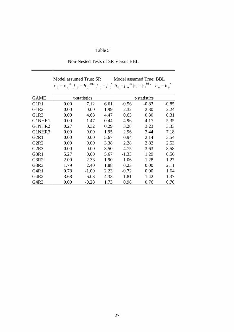
estimated in conjunction with α. Table 5 contains the absolute value of the t-statistics
for testing the hypothesis α = 0 for each of the 15 sets of experiments. In discussing
these tests, the null is evaluated using a symmetric test at the nominal 5% level.
Summaries of the tests are shown in Figure 3. For example, the 12 acceptances of the
SR model in panel (a) correspond to the 12 times the t- statistic in the first column of
Table 5 is less than the critical value 1.96.
Figure 3 shows that the choice of how propensities or attractions are updated has a
large influence on the test results. When ϕ β ϕ0 0= = SR , as in (a), the data accept SR in
12 of 15 cases. When ϕ β β0 0= = BBL , as it does in Figure 3, the evidence is less
favorable to SR. Now SR is accepted in 10 of 15 cases, while BBL is accepted in 8 of
15. But when the estimates of β 0 and ϕ 0 are unconstrained, ϕ ϕ0 0= * and β β0 0= * , as
in the artificial regressions summarized in (c), the evidence supporting either theory is
equivocal. In 6 of 15 cases SR is accepted, and in 7 cases BBL is accepted. Ignoring
the 2 cases where both models are accepted and the 4 cases where both models are
rejected, leaves 4 cases where SR is accepted and BBL rejected, and precisely 5 cases
where the reverse is true. Thus the data render a Scotch verdict: the case for either
model is not proved.
There is a pattern in the tests that suggests an explanation for these results. Three of
the 4 cases that support SR and reject BBL all come from the experiments G1NH.
These are the experiments where history of play information was not made available to
senders or receivers. Consequently, the case for SR behavior is strongest here.
Similarly, 2 of the 5 cases that support BBL and reject SR come from the G1
experiments where information about the history of play was made available. In these

13
experiments a stronger a priori case for BBL can be made. Thus, it appears that the
structure of the experiment has an important effect upon the modality of learning
behavior that occurs for Game 1.
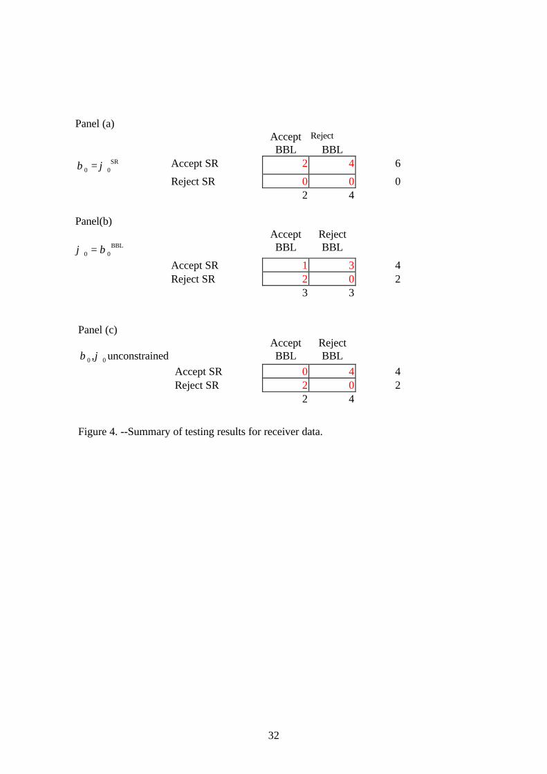
We also examined receiver behavior. Unlike senders, receivers actually have the
information that is needed to engage in forms of learning like fictitious play. Thus a
comparison between sender and receiver learning can inform us about the importance of
the type of information that is available at the population level. A direct comparison
between sender and receiver behavior is not possible for all experiments because
receivers frequently had more actions that they could take. However, for Game1, both
with and without information on history of play, both senders and receivers faced binary
choices and a comparison could be made. Generally, the results for the receiver data
looked much like the sender data. Both SR and BBL models fit the data well, with SR
doing slightly better in the games with no history, and BBL doing better where history of
play information was available. The average difference in R2 was 0.03 across the six
games/replications. Figure 4 summarizes the six experimental results. Overall, the test
results in Panel (c) of the figure show SR being the preferred model in 4 of the 6 cases,
with BBL the preferred model in the other two cases, both of which were from the
games with history of play information available. Though consistent with a learning
story, this is only weak evidence in favor of one model, and underscores our point that it
is difficult to tell these models apart with any degree of precision.
IV. HYBRID MODEL
In this section, the approach of Camerer and Ho (1997) is adapted to our
experimental data. The updating equation which defines the propensity Qij(t) of player i
to play action j at time t is now modified to include both own and population average
payoffs:
(7) Q t Q t X t X tij ij ij j( ) ( ) ( ) ( )= − + − + −γ γ γ0 1 21 1 1

14
where Xij(t-1) is the reward player i receives from taking action j at time t-1 and Xj
(t-1) is the average reward all players except i received from taking action j at time t-1.
We refer to the model with the updating equation (7) as the hybrid model since it is a
combination of the SR and BBL models.4
The likelihood function for the sender data was maximized separately for each of the
15 replications using observations from round 2 onwards. As with the previous models,
maximization can be achieved by Iteratively Re-Weighted Least Squares, which provides
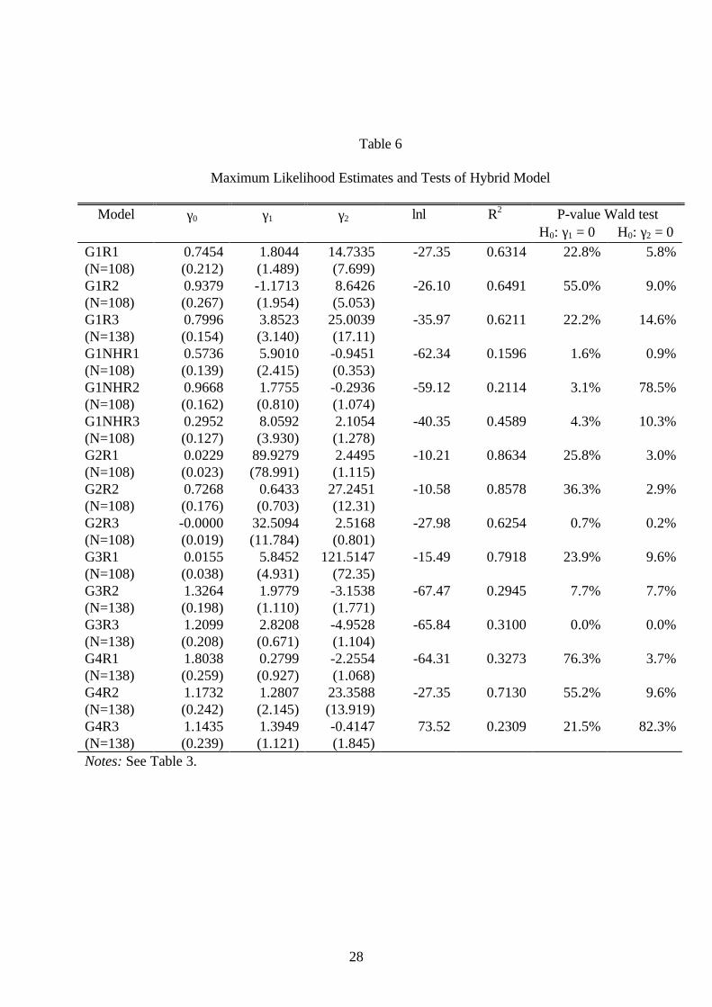
measures of fit for the non-linear regression. The results of maximization are shown in
Table 6. Columns 2, 3 and 4 of the table contain the estimates of γ0, γ1 and γ2 and
column 5 contains the log likelihood value at its optimum. Columns 6 and 7 contain the
Wald t statistics for testing the hypotheses H0: γ1 = 0 and H0: γ2 = 0. Each null
hypothesis is evaluated using a symmetric test at the nominal 5% level.
Consider the contribution of own payoff information given that the model contains
the information on the population average payoff. For the common interest games (G1
and G2), the ones with a unique efficient payoff point, own payoff information only
matters under the no-history condition, which is intuitively plausible and consistent with
the results from the non-nested comparison. For the divergent interest games (G3 and
G4), the ones with a conflict of interest between senders and receivers, the contribution
of own payoff information is statistically significant in only 1 of 6 cases. Next we turn to
the contribution of population average payoff information given that the model contains
information on own payoffs. Population average payoff information is significant in the
common interest games only in Game 2, with the possible exception of G1R1. The BBL
story suggests that population average payoff information should be significant in all
games where it is available. This includes Game1 and also the divergent interest games.
It is significant in 2 of 6 cases for the divergent interest games, but with a negative sign,
4 The coefficients in the hybrid model can be normalized so that the coefficients on the information
variables are δ and (1- δ), respectively, which makes the hybrid model look similar to the modelemployed Camerer and Ho (1997). Estimating the initial condition, δ0 and δ, where δ0 is thecoefficient of the lagged propensity, is equivalent to estimating γ0, γ1 and γ2 while fixing theinitial condition.

15
which is contrary to BBL. This may be evidence for sophisticated learning, namely,
senders trying to counteract the evolution of meaning of messages in the population.
The results appear to be strongly influenced by multicollinearity between the own
payoff variable and the population average payoff variable. One source of the
multicollinearity is that the population average payoff contains the own payoff of player
j, for each j. We re-estimated the hybrid model using a definition of the population
average payoff that excludes the own payoff of player j for each j. This substantially
changed the estimates and standard errors for many of the experiments. On the other
hand, the test results are more or less similar to those above, but with less support for
either SR or BBL.
Another source of multicollinearity is due to learning. If play converges to a pure
strategy equilbrium, then the own payoff and population average payoff variables take on
identical values. Thus, after convergence to equilbrium there is exact collinearity between
the two information variables. Multicollinearity tends to be more of a problem in the
common interest games, although G3R1 presents a striking example in the case of the
divergent interest games as indicated by its enormous standard error. The degree of
multicollinearity depends on the number of observations included in the data after
convergence has been achieved. This matter is discussed in more detail in the following
section.
V. CONVERGENCE BIAS
It is common practice to include all observations from a particular experiment in any
statistical estimation or testing exercise based on that experiment. Yet information about
learning can only come from observations where learning occurs. Once behavior has
converged, observations have no further information about learning. Including such
observations will make the model appear to „fit“ better, while at the same time reducing
the contrast between models, making it difficult to distinguish the models empirically.
The data shown in Figures 1 and 2 indicate that convergence typically occurs within 5 to

16
7 rounds, while observations are included in the estimation for the entire period, in these
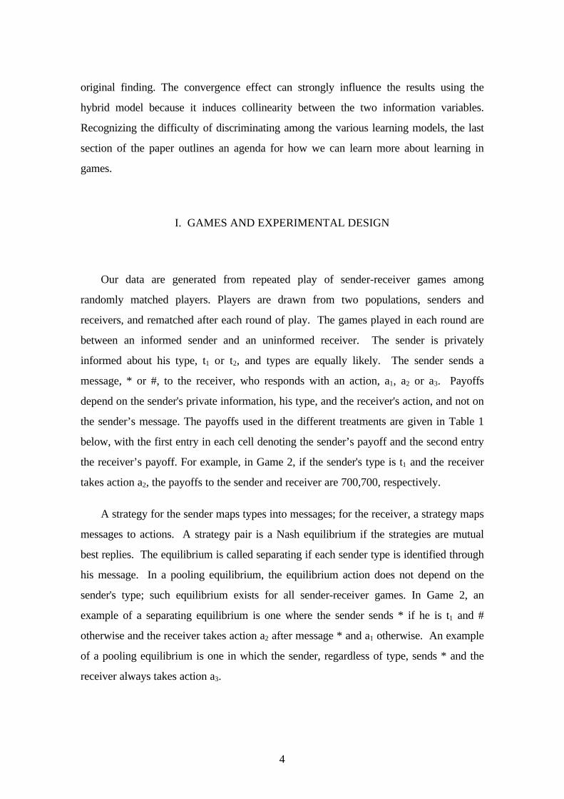
data up to 20 periods. To illustrate the possible bias that this might cause we calculated
R2 and average log likelihood (the maximized log likelihood/ # of observations used) by
progressively removing observations from the later periods, that is, by removing
observations that include convergence. Figure 5 illustrates this bias for the experiments
of Game 1. The lines show the comparison between SR (triangles) and BBL (circles) for
a specified number of included rounds Under the hypothesis of no convergence bias we
would expect the slopes of each line in panels (a) and (b) of the figure to have zero
slope. In fact, all four lines have positive slope, which is characteristic of convergence
bias. However, the difference between the lines in each panel is approximately constant
in these data, which suggests that convergence bias makes both models appear to fit the
data better, but does not otherwise bias the comparison of SR and BBL.
To measure the amount of bias requires taking a position on when convergence has
occurred, a classification that is better made on individual data. We define the
convergence operator Tp(yit) by
(8) T y if y y yp it it it it p( ) ...= = = =− −1 1
= 0 else
In other words a player's (pure) strategy is said to have converged if the same action
is taken p times in a row.5 To eliminate convergence bias one simply excludes
observation where Tp=1. We used this procedure with p = 3 and p = 4 to assess the
extent of this bias. We found that at least for these data, the extent of the bias was small.
For example, the non-nested hypothesis tests shown in Figure 3(c) had the same off-
diagonal values (3), while the accept-accept entry changed from 5 to 4, while the reject-
reject entry changed from 4 to 5. In other words, correcting for convergence bias
sharpened the distinction between the two models but it did not favor either model.
5 Defining convergence for mixed strategies is conceptually the same as the pure strategy case;
empirically identifying convergence is more difficult.
17
VI. RELATED LITERATURE
There is an extensive and growing literature in experimental economics on learning.
For example, see Richard T. Boylan and Mahmoud A. El-Gamal (1993), Camerer and
Ho (1997), Cheung and Friedman (1997), David J. Cooper and Nick Feltovich (1996),
James C. Cox, Jason Shachat and Mark Walker (1995), Vincent P. Crawford (1995),
Roth and Erev (1995). The literature generally focuses on two broad classes of learning
models, stimulus-response and belief based play. A wide variety of games are considered
with various designs, e.g., whether or not players are provided with the history of the
game. The performances of the learning models are evaluated using simulation and
various statistical techniques. Unfortunately, the findings are mixed at best. This could
be due to statistical issues, Drew Fudenberg and David K. Levine's (1997) conjecture
that with convergence to Nash in the "short term," the models maybe indistinguishable,
or a combination of the two.
Roth and Erev (1995) focus on the stimulus-response model. Their concern is high
(super rationality) versus low (stimulus-response) game theory and intermediate (e.g.,
Fudenberg and Levine’s „short term“) versus asymptotic results. Their model is a simple
individual reinforcement dynamic in which propensities to play a strategy are updated
based upon success of past play. Using simulation, they avoid the problem of estimation
and compare the simulations to their experiments. The simulated outcomes are similar to
observed behavior and, more importantly, vary similarly across the different games
considered. They interpret this as robustness of the intermediate run outcomes to the
chosen learning rule. Comparisons have also been made between the stimulus-response
model of Roth and Erev or similar reinforcement dynamics (e.g., Robert R. Bush and
Frederick Mosteller (1955) and John G. Cross (1983) and other learning models. Using
logit, simulation or other statistical techniques, the general conclusions of these papers
are that stimulus-response works well and that additional information when part of the
design makes a difference, Dilip Mookherjee and Barry Sopher (1994, 1997), Ido Erev
and Amnon Rapoport (1998) and Ido Erev and Alvin E. Roth (1997) .
18
Using a variety of games and an information condition (with and without game
history) in an extended probit, Cheung and Friedman’s (1997) find that the belief based
model has more support than stimulus-response learning and information matters. Boylan
and El-Gamal (1993) find that fictitious play is the overwhelming choice when compared
with Cournot learning in their evaluation. Using the standard logit model, Van Huyck et
al. (1997) focus on symmetric coordination games and evaluate the performance of the
replicator dynamic, fictitious and exponential fictitious play. Exponential fictitious play
does best. Models of reinforcement learning can be used to justify the replicator dynamic
(e.g., Tilman Boergers and Rajiv Sarin (1995)).
Richard D. McKelvey and Thomas R. Palfrey’s (1995) model of quantal response
equilibria in normal form games deserves attention here. The quantal response model is
Nash with error. Using the logit model, they find that the quantal response model wins
when compared to Nash without error and random choice. Important for us is their
conclusion that errors are an important component in explaining experimental results.
This has been implicitly assumed in the previous studies when logits and probits are used
and explicitly assumed in the Erev and Roth (1997) study with simulations.
The lack of general findings in these and other papers has prompted Camerer and
Ho (1997) to essentially give up on the horse race and develop a general model, which
has as special cases the principal learning models in the literature.6 The key that ties the
SR models to the BBL models is the reinforcement used. In the SR model, only actions
that were taken are updated based on the actual payoffs, and in the BBL model every
action is updated based on its hypothetical payoff, that is, the payoff it would receive had
the action been taken. When actual and hypothetical payoffs are the same so are the
models. Using maximum likelihood estimation under the constraints of logit, Camerer
and Ho evaluate the possible contribution of the general model across a variety of games.
As one would hope, the general model explains more of the variation.
6 The number of studies is growing at an increasing rate. We have selected representatives from the
set and apologize for any omissions.

19
Reinhard Selten (1997) is the true agnostic. He claims there is not enough data to
form any conclusions, either theoretical or statistical. The best we can do is very general
qualitative models (e.g., learning direction theory) in which there are tendencies that are
distinct from random behavior but nothing more. This view brings us full circle to
Fudenberg and Levine’s conjecture about whether you can distinguish among the models
if equilibrium play is observed in the „short term“ or alternatively, the statistical issues
make such comparisons moot.
The resolution of this debate is ultimately an empirical one. Based on the data in this
paper, we find that it is difficult to discriminate between the SR and BBL models. In
general, it appears that care must be exercised when constructing the statistics for the
horse races and simulation comparisons that are made.
VII. SUMMARY AND FUTURE AGENDA
In this paper we investigated how well SR and BBL models describe learning in a
sender-receiver game experiment. In the experiment an extensive form game is played
repeatedly among players who are randomly matched before each round of play. This
population-game environment is particularly appropriate for a comparison of myopic
learning rules, if we believe that it lessens the role of repeated game strategies. Sender-
receiver games with costless and a priori meaningless messages have the advantage that
no matter how we specify the incentives, coordination requires learning. One
consequence of studying learning in extensive form games is that since players in the
experiment observe only each others’ actions, not strategies, the principal difference
between the two learning models is in the roles they assign to own experience versus
population experience. Another consequence is that there are different natural
specifications even for a learning model as simple as SR; we chose the cognitively least
demanding one, in which experience at one information set does not transfer to other
information sets.

20
We found that both models fit our data well and the predicted choice probabilities
closely track the actual choice frequencies. It is suggestive that the BBL model fits
slightly better than SR when population information is available, and vice versa without
such information. However the differences are not large enough to be conclusive. When
the SR and BBL models were compared using a well-known non-nested testing
procedure, we found that depending on parameter choices, this test may favor either
model. If parameters are unrestricted, both models are approximately equally often
accepted and rejected. Thus, like the comparison of fits, this formal test does not permit
us to choose one model over the other. When the SR and BBL models were compared
to a hybrid model, the data did not clearly favor one over the other. We raise the issue of
convergence bias and show that for our data correcting for this bias does not lead to
better discrimination between the two models.
The issue raised by our experimental results and those of others is how to learn more
from experiments. The starting point for our agenda for the future is based on the fact
that learning models in games specify the data generating process. As a consequence, the
models can be simulated. This opens up the possibility of investigating problems of
optimal experimental design in game theory. The first point to note is that our treatment
of testing with experimental data has been, from a statistical point of view, entirely
conventional. We have assumed that standard asymptotic theory provides a reliable
guide for inference in models with sample sizes encountered in experimental economics.
Of course, approximations based on asymptotic theory may be poor for sample sizes
typically used in practice. In particular, the true probability of making a Type I error
may be very different than the nominal probability. The simulated data can be used to
estimate the probability of making a Type I error for tests based on asymptotic critical
values. If asymptotic critical values do not work, then the performance of other
approximations can be investigated, for example, bootstrap-based critical values. Once
the probability of making a Type I error is under control, the powers of the tests can be
examined. This will tell the sample size needed to be able to discriminate between the
models. Finally, considerations of power lead to an optimal design framework, a
framework that will enable us to design our experiments so as to learn about learning.

21
REFERENCES
Austen-Smith, David; „Information Transmission in Debate,“ American Journal ofPolitical Science, February 1990, 34(1), pp. 124-152.
Blume, Andreas; DeJong, Douglas V., Kim, Yong-Gwan and Sprinkle Geoffrey.„Experimental Evidence on the Evolution of the Meaning of Messages in Sender-Receiver Games.“ Forthcoming American Economic Review 1998.
Boergers, Tilman and Sarin, Rajiv. "Learning Through Reinforcement and ReplicatorDynamics," unpublished manuscript, University College London. 1995.
Boylan, Richard T. and El-Gamal, Mahmoud A. "Fictitious Play: A Statistical Study ofMultiple Economic Experiments," Games and Economic Behavior, April 1993, 5(2), pp. 205-222.
Bush, Robert R. and Mosteller, Frederick. Stochastic Models of Learning, New York:Wiley, 1955.
Camerer, Colin and Ho, Teck-Hua. „Experience-weighted Attraction Learning inGames: A Unifying Approach“, Cal Tech Social Science working paper 1003,California Institute of Technology. 1997.
Cheung, Ying-Wong and Friedman, Daniel. „Individual Learning in Normal FormGames: Some Laboratory Results,“ Games and Economic Behavior, April 1997,19(1), pp. 46-79.
_____ „A Comparison of Learning and Replicator Dynamics Using ExperimentalData,“, University of California at Santa Cruz working paper, University ofCalifornia at Santa Cruz, October 1996.
.Cooper, David J. and Feltovich, Nick. „Reinforcement-Based Learning vs. Bayesian
Learning: A Comparison,“ University of Pittsburgh working paper, University ofPittsburgh. 1996,
Cox, James C.; Shachat, Jason and Walker, Mark. „An Experiment to Evaluate BayesianLearning of Nash Equilibrium,“ University of Arizona working paper, Universityof Arizona. 1995
Crawford, Vincent P.„Adaptive Dynamics in Coordination Games,“ Econometrica,January 1995, 63(1), pp.103-143.
Crawford,Vincent P. and Sobel, Joel. „Strategic Information Transmission,“Econometrica, November 1982, 50(6), pp. 1431-1452.

22
Cross, John G. A Theory of Adaptive Economic Behavior, Cambridge:CambridgeUniversity Press. 1983.
Davidson, Russell and MacKinnon, James G. „Convenient Specification Tests for Logitand Probit Models,“ Journal of Econometrics, July 1984, 25(3), pp. 241-62.
______ Estimation and Inference in Econometrics, Oxford, University of Oxford Press.1993.
Erev, Ido. „Signal Detection by Human Observers: A Cutoff Reinforcement LearningModel of Categorization Decisions under Uncertainty,“ Technion working paper,Technion. 1997.
Erev, Ido and Rapoport, Amnon. „Coordination, „Magic,“ and Reinforcement Learningin a Market Entry Game.“ Games and Economic Behavior, May 1998, 23(2), pp.146-175.
Erev, Ido and Roth, Alvin E. „Modeling How People Play Games: ReinforcementLearning in Experimental Games with Unique, Mixed Strategy Equilibria,“University of Pittsburgh working paper, University of Pittsburgh. 1997.
Farrell, Joseph and Gibbons, Robert. „ Union Voice,“ Cornell University working paper,Cornell University, 1990.
Fudenberg, Drew and Kreps, David M. „Learning Mixed Equilibria,“ Games andEconomic Behavior, July 1993, 5(3), pp. 320-67..
Fudenberg, Drew and Levine, David K. Theory of Learning in Games, Cambridge: MITPress. 1998.
Gigler, Frank. „Self-Enforcing Voluntary Disclosures,“ Journal of Accounting Research,Autum 1994, 32(2), pp. 224-240.
McFadden, Daniel, "Conditional Logit Analysis of Qualitative Choice Behavior," in PaulZarembka, ed., Frontiers in Econometrics, New York, Academic Press. 1974.
McKelvey, Richard D. and Palfrey, Thomas R. "Quantal Response Equilibria for NormalForm Games," Games and Economic Behavior, July 1995, 10(1), pp. 6-38.
Mookherjee, Dilip and Sopher, Barry. "Learning Behavior in an Experimental MatchingPennies Game," Games and Economic Behavior, July 1994, 7(1), pp. 62-91.
"Learning and Decision Costs in Experimental Constant Sum Games. Games andEconomic Behavior, April 1997, 19(1), pp. 97-132.
Robinson, Julia. „An Iterative Method of Solving a Game,“ Annals of Mathematics,September 1951, 54(2), pp. 296-301.

23
Roth, Alvin E. and Erev, Ido. „Learning in Extensive Form Games: Experimental Dataand Simple Dynamic Models in the Intermediate Term,“ Games and EconomicBehavior, January 1995, 8(1), pp. 164-212.
Selten, Reinhard. "Features of Experimentally Observed Bounded Rationality,"Presidential Address, European Economic Association, Toulouse. 1997.
Stein, Jeremy. „Cheap Talk and the Fed: A Theory of Imprecise PolicyAnnouncements,“ American Economic Review, March 1989, 79(1), pp. 32-42.
Van Huyck, John B.; Battalio, Raymond C., and Rankin, Frederick W. „On the Origin ofConvention: Evidence from Coordination Games,“ Economic Journal, May1997, 107, pp. 576-596.
24
Table 1− Payoffs of Games in Experiments
Panel (a)Actions
Types Game 1 Game 2a1 a2 a1 a2 a3
t1 0,0 700,700 0,0 700,700 400,400t2 700,700 0,0 700,700 0,0 400,400
Panel (b)Actions
Types Game 3 Game 4a1 a2 a3 a1 a2 a3
t1 0,0 200,700 400,400 0,0 200,500 400,400t2 200,700 0,0 400,400 200,500 0,0 400,400
.
Table 2- Experimental Treatments
Game Session Data PopulationHistory
Number ofPeriods
G1 Game 1 Session II Senders 20G1NH Game 1 Session II No history 20G2 Game 2 Session II Senders 20G3 Game 3 Session II Senders 40G4 Game 4 Session II Senders 40
Notes: In the analysis of the experimental data only the first 25 periods are used for G3and G4.

25
Table 3
Maximum Likelihood Estimates of SR Model
Model ϕ0 ϕ1 lnl R2 LR-statistic P-valueG1R1(N=108)
0.4320(0.143)
0.7352(0.636)
-34.48 .5353 14.9 0.0%
G1R2(N=108)
0.5785(0.138)
1.1762(0.783)
-25.50 .6572 6.7 0.1%
G1R3(N=138)
0.5787(0.153)
1.1203(1.026)
-42.52 .5522 7.9 0.0%
G1NHR1(N=108)
0.6299(0.099)
0.8044(0.514)
-49.25 .3362 9.4 0.2%
G1NHR2(N=108)
0.9499(0.118)
1.3059(0.809)
-57.32 .2341 0.2 64.8%
G1NHR3(N=108)
0.6494(0.096)
1.0801(0.601)
-40.37 .4585 7.8 0.1%
G2R1(N=108)
0.2793(0.151)
0.8798(0.769)
-13.67 .8172 19.6 0.0%
G2R2(N=108)
0.0228(0.029)
0.0048(0.164)
-11.63 .8437 9.6 0.2%
G2R3(N=108)
0.2352(0.184)
0.9473(1.062)
-13.73 .8162 14.0 0.0%
G3R1(N=108)
0.5485(0.302)
8.7117(11.69)
-20.32 .7268 0.8 35.8%
G3R2(N=138)
0.8206(0.099)
2.0399(1.312)
-69.30 .2753 1.7 18.9%
G3R3(N=138)
0.9661(0.108)
2.7681(1.552)
-63.21 .3375 0.2 65.5%
G4R1(N=138)
0.6151(0.098)
0.2335(0.203)
-70.01 .6472 15.6 0.0%
G4R2(N=138)
0.6216(0.132)
4.6780(3.582)
-30.53 .6795 2.5 11.6%
G4R3(N=138)
0.6737(0.083)
0.5778(0.437)
-75.62 .2089 7.3 0.7%
Notes: N = 6 times the number of periods (20 or 25) minus 12. Standard errors inparentheses beneath coefficient estimates.
26
Table 4
Maximum Likelihood Estimates of BBL Model
Model β0 β1 lnl R2 LR-statistic P-valueG1R1(N=108)
0.7384(0.208
13.6086(5.890)
-27.36 .6313 1.09 29.6%
G1R2(N=108)
0.6565(0.260)
6.8891(3.017)
-26.81 .6396 0.0 99.9%
G1R3(N=138)
0.8013(0.152)
24.1275(12.72)
-35.95 .6214 1.7 19.8%
G1NHR1(N=108)
1.1917(0.270)
2.0617(1.897)
-56.76 .2349 0.9 34.9%
G1NHR2(N=108)
0.9784(0.183)
2.6596(1.596)
-61.71 .1754 0.7 93.5%
G1NHR3(N=108)
0.5522(0.183)
6.9908(2.690)
-44.04 .4094 10 30.6%
G2R1(N=108)
0.0987(0.072)
43.8475(22.640)
-13.53 .8191 5.7 1.7%
G2R2(N=108)
0.2904(0.126)
25.380)(8.951)
-11.11 .8507 0.3 60.5%
G2R3(N=108)
0.3912(0.139)
17.6949(5.647)
-14.05 .8119 0.5 47.9%
G3R1(N=108)
0.0034(0.013)
79.9333(34.02)
-15.53 .7911 6.9 0.9%
G3R2(N=138)
1.1704(0.173)
2.3093(1.834)
-67.43 .2949 0.1 78.2%
G3R3(N=138)
1.9416(0.183)
-2.5189(0.382)
-64.48 .3242 10.5 0.1%
G4R1(N=138)
1.8391(0.255)
-1.2460(0.791)
-64.35 .3269 13.3 0.0%
G4R2(N=138)
1.0740(0.219)
17.4783(8.373)
-27.12 .7153 0.2 68.9%
G4R3(N=138)
1.3106(0.228)
0.7460(1.493)
-73.96 .2263 2.2 13.4%
Notes: See Table 3.
27
Table 5
Non-Nested Tests of SR Versus BBL
Model assumed True: SR Model assumed True: BBL
ϕ ϕ0 0= SR ϕ β0 0= BBL ϕ ϕ0 0= * β ϕ0 0= SR β β0 0= BBL β β0 0= *
GAME t-statistics t-statisticsG1R1 0.00 7.12 6.61 -0.56 -0.83 -0.85G1R2 0.00 0.00 1.99 2.32 2.30 2.24G1R3 0.00 4.68 4.47 0.63 0.30 0.31G1NHR1 0.00 -1.47 0.44 4.96 4.17 5.35G1NHR2 0.27 0.32 0.29 3.28 3.23 3.33G1NHR3 0.00 0.00 1.95 2.96 3.44 7.18G2R1 0.00 0.00 5.67 0.94 2.14 3.54G2R2 0.00 0.00 3.38 2.28 2.82 2.53G2R3 0.00 0.00 3.50 4.75 3.63 8.58G3R1 5.27 0.00 5.67 -1.33 1.29 0.56G3R2 2.00 2.33 1.90 1.06 1.28 1.27G3R3 1.79 2.40 1.88 0.23 0.00 2.11G4R1 0.78 -1.00 2.23 -0.72 0.00 1.64G4R2 3.68 6.03 4.33 1.81 1.42 1.37G4R3 0.00 -0.28 1.73 0.98 0.76 0.70
28
Table 6
Maximum Likelihood Estimates and Tests of Hybrid Model
Model γ0 γ1 γ2 lnl R2 P-value Wald testΗ0: γ1 = 0 Η0: γ2 = 0
G1R1(N=108)
0.7454(0.212)
1.8044(1.489)
14.7335(7.699)
-27.35 0.6314 22.8% 5.8%
G1R2(N=108)
0.9379(0.267)
-1.1713(1.954)
8.6426(5.053)
-26.10 0.6491 55.0% 9.0%
G1R3(N=138)
0.7996(0.154)
3.8523(3.140)
25.0039(17.11)
-35.97 0.6211 22.2% 14.6%
G1NHR1(N=108)
0.5736(0.139)
5.9010(2.415)
-0.9451(0.353)
-62.34 0.1596 1.6% 0.9%
G1NHR2(N=108)
0.9668(0.162)
1.7755(0.810)
-0.2936(1.074)
-59.12 0.2114 3.1% 78.5%
G1NHR3(N=108)
0.2952(0.127)
8.0592(3.930)
2.1054(1.278)
-40.35 0.4589 4.3% 10.3%
G2R1(N=108)
0.0229(0.023)
89.9279(78.991)
2.4495(1.115)
-10.21 0.8634 25.8% 3.0%
G2R2(N=108)
0.7268(0.176)
0.6433(0.703)
27.2451(12.31)
-10.58 0.8578 36.3% 2.9%
G2R3(N=108)
-0.0000(0.019)
32.5094(11.784)
2.5168(0.801)
-27.98 0.6254 0.7% 0.2%
G3R1(N=108)
0.0155(0.038)
5.8452(4.931)
121.5147(72.35)
-15.49 0.7918 23.9% 9.6%
G3R2(N=138)
1.3264(0.198)
1.9779(1.110)
-3.1538(1.771)
-67.47 0.2945 7.7% 7.7%
G3R3(N=138)
1.2099(0.208)
2.8208(0.671)
-4.9528(1.104)
-65.84 0.3100 0.0% 0.0%
G4R1(N=138)
1.8038(0.259)
0.2799(0.927)
-2.2554(1.068)
-64.31 0.3273 76.3% 3.7%
G4R2(N=138)
1.1732(0.242)
1.2807(2.145)
23.3588(13.919)
-27.35 0.7130 55.2% 9.6%
G4R3(N=138)
1.1435(0.239)
1.3949(1.121)
-0.4147(1.845)
73.52 0.2309 21.5% 82.3%
Notes: See Table 3.

29
Experiment = G1R1
round1 5 10 15
.1
.3
.5
.7
.9
1 1 1
1 1
1 1 1 1 1 1 1
2
2 2 2
2
2
2 2 2 2 2 2 2
Experiment = G1R2
round1 5 10 15
.1
.3
.5
.7
.9
1
1
1
1
1
1 1
1
1 1 1 1
2 2
2
2
2
2 2 2 2 2 2 2 2
Experiment = G1R3
round1 5 10 15
.1
.3
.5
.7
.9
1
1
1 1 1 1
1 1
1
1 1 1 1 1 1
2
2 2
2 2
2
2 2
2 2 2 2 2
Experiment = G1NHR1
round1 5 10 15
.1
.3
.5
.7
.9
1
1
1 1
1
1
1
1
1
1
1
1
2
2
2
2
2
2
2
2
2
2 2 2
Experiment = G1NHR2
round1 5 10 15
.1
.3
.5
.7
.9
1 1
1
1 1
1
1
1
1
1
1 1
2
2
2
2
2
2 2
2
2
2 2
2
2
Experiment = G1NHR3
round1 5 10 15
.1
.3
.5
.7
.9
1
1 1
1
1 1
1
1 1 1
2
2 2
2
2
2
2 2
2
2
2
2
Experiment = G2R1
round1 5 10 15
.1
.3
.5
.7
.9
1 1 1
1 1
1
1 1 1 1 1 1 1
2
2 2
2 2 2 2 2 2 2 2 2 2
Experiment = G2R2
round1 5 10 15
.1
.3
.5
.7
.9
1 1
1
1 1 1 1 1 1 1 1 1 1 1
2
2 2 2 2 2 2 2 2 2 2 2 2 2 2
Experiment = G2R3
round1 5 10 15
.1
.3
.5
.7
.9
1
1 1 1 1
1 1 1 1 1 1 1 1
2
2
2 2 2 2 2 2 2 2 2 2
Experiment = G3R1
round1 5 10 15
.1
.3
.5
.7
.9
1 1
1 1
1
1 1 1 1 1 1 1 1 1
2
2 2 2 2 2 2 2
2
2 2
Experiment = G3R2
round1 5 10 15
.1
.3
.5
.7
.9
1 1
1
1 1 1 1 1
1
1
1
1
1
1
1
2
2
2
2 2
2 2 2
2 2
2
2
2
2
2
Experiment = G3R3
round1 5 10 15
.1
.3
.5
.7
.9
1
1
1
1
1
1
1
1
1
1
1
1
1
1 1 1 1 1 1 1
2
2
2
2
2
2
2 2
2
2
2
2
2
2
2 2
2
Experiment = G4R1
round1 5 10 15
.1
.3
.5
.7
.9
1
1
1
1
1
1 1 1
1
1
1 1
1
1 1
2
2
2
2
2
2
2 2 2
2
2 2
2
2 2
Experiment = G4R2
round1 5 10 15
.1
.3
.5
.7
.9
1 1
1 1 1 1 1 1 1 1
1 1
1
1
1 1 1
2 2
2 2
2 2
2 22 2 2
2
2 2
2
Experiment = G4R3
round1 5 10 15
.1
.3
.5
.7
.9
1
1
1 1 1
1 1
1
1
1
1
1
1 1 1
1
2 2
2
2
2
2
2
2
2
2
2 2
2
2
Figure 1.—Plots of the actual and predicted fraction of players sending message 2 bytype when the SR model is true.

30
Experiment = G1R1
round1 5 10 15
.1
.3
.5
.7
.9
1 1 1
1 1
1 1 1 1 1 1 1
2
2 2 2
2
2
2 2 2 2 2 2 2
Experiment = G1R2
round1 5 10 15
.1
.3
.5
.7
.9
1
1
1
1
1
1 1
1
1 1 1 1
2 2
2
2
2
2 2 2 2 2 2 2 2
Experiment = G1R3
round1 5 10 15
.1
.3
.5
.7
.9
1
1
1 1 1 1
1 1
1
1 1 1 1 1 1
2
2 2
2 2
2
2 2
2 2 2 2 2
Experiment = G1NHR1
round1 5 10 15
.1
.3
.5
.7
.9
1
1
1 1
1
1
1
1
1
1
1
1
2
2
2
2
2
2
2
2
2
2 2 2
Experiment = G1NHR2
round1 5 10 15
.1
.3
.5
.7
.9
1 1
1
1 1
1
1
1
1
1
1 1
2
2
2
2
2
2 2
2
2
2 2
2
2
Experiment = G1NHR3
round1 5 10 15
.1
.3
.5
.7
.9
1
1 1
1
1 1
1
1 1 1
2
2 2
2
2
2
2 2
2
2
2
2
Experiment = G2R1
round1 5 10 15
.1
.3
.5
.7
.9
1 1 1
1 1
1
1 1 1 1 1 1 1
2
2 2
2 2 2 2 2 2 2 2 2 2
Experiment = G2R2
round1 5 10 15
.1
.3
.5
.7
.9
1 1
1
1 1 1 1 1 1 1 1 1 1 1
2
2 2 2 2 2 2 2 2 2 2 2 2 2 2
Experiment = G2R3
round1 5 10 15
.1
.3
.5
.7
.9
1
1 1 1 1
1 1 1 1 1 1 1 1
2
2
2 2 2 2 2 2 2 2 2 2
Experiment = G3R1
round1 5 10 15
.1
.3
.5
.7
.9
1 1
1 1
1
1 1 1 1 1 1 1 1 1
2
2 2 2 2 2 2 2
2
2 2
Experiment = G3R2
round1 5 10 15
.1
.3
.5
.7
.9
1 1
1
1 1 1 1 1
1
1
1
1
1
1
1
2
2
2
2 2
2 2 2
2 2
2
2
2
2
2
Experiment = G3R3
round1 5 10 15
.1
.3
.5
.7
.9
1
1
1
1
1
1
1
1
1
1
1
1
1
1 1 1 1 1 1 1
2
2
2
2
2
2
2 2
2
2
2
2
2
2
2 2
2
Experiment = G4R1
round1 5 10 15
.1
.3
.5
.7
.9
1
1
1
1
1
1 1 1
1
1
1 1
1
1 1
2
2
2
2
2
2
2 2 2
2
2 2
2
2 2
Experiment = G4R2
round1 5 10 15
.1
.3
.5
.7
.9
1 1
1 1 1 1 1 1 1 1
1 1
1
1
1 1 1
2 2
2 2
2 2
2 22 2 2
2
2 2
2
Experiment = G4R3
round1 5 10 15
.1
.3
.5
.7
.9
1
1
1 1 1
1 1
1
1
1
1
1
1 1 1
1
2 2
2
2
2
2
2
2
2
2
2 2
2
2
Figure 2.—Plots of actual and predicted fractions of players sending message 2 by typewhen the BBL model is true.

31
Panel (a)Accept RejectBBL BBL
β ϕ0 0= SR Accept SR 6 6 12
Reject SR 3 0 39 6
Panel(b)Accept Reject
ϕ β0 0= BBL BBL BBL
Accept SR 3 7 10Reject SR 5 0 5
8 7
Panel (c)Accept Reject
β ϕ0 0, unconstrained BBL BBL
Accept SR 2 4 6Reject SR 5 4 9
7 8
Figure 3. --Summary of testing results for sender data
32
Panel (a)Accept Reject
BBL BBL
β ϕ0 0= SR Accept SR 2 4 6
Reject SR 0 0 02 4
Panel(b)Accept Reject
ϕ β0 0= BBL BBL BBL
Accept SR 1 3 4Reject SR 2 0 2
3 3
Panel (c)Accept Reject
β ϕ0 0, unconstrained BBL BBL
Accept SR 0 4 4Reject SR 2 0 2
2 4
Figure 4. --Summary of testing results for receiver data.

33
Panel (b)
Panel (a)R-Square Comparison By ModelExperiment = Game 1
Included Rounds7 9 11 13
.6
.7
.8
.9
1
Log Likelihood Comparison By ModelExperiment = Game 1
Included Rounds7 9 11 13
-.5
-.4
-.3
-.2
Figure 5—Convergence bias:Ο --BBL;∆ --SR
Copyright © 2022 FDOKUMEN

