


Bahasa
Halaman
Hukum

Southeast Asia
Landscape Dynamics Over Time and
Space From Ecological Perspective
Sonya Dewi and Andree Ekadinata

Landscape dynamics over time and space from an ecological perspective
Sonya Dewi and Andree Ekadinata
Working Paper 103
- ii -
Citation
Dewi S, Ekadinata A. 2010. Landscape dynamics over time and space from an ecological perspective.
Working paper 103. Bogor, Indonesia: World Agroforestry Centre (ICRAF) Southeast Asia Program.
Titles in the working paper series disseminate interim results on agroforestry research and practices to
stimulate feedback from the scientific community. Other publication series from the World
Agroforestry Centre include agroforestry perspectives, technical manuals and occasional papers.
Published by
World Agroforestry Centre (ICRAF)
Southeast Asia Regional Office
PO Box 161, Bogor 16001, Indonesia
Tel: +62 251 8625415
Fax: +62 251 8625416
Email: [email protected]
http://www.worldagroforestrycentre.org/sea
© World Agroforestry Centre 2010 Working Paper 103
Disclaimer and copyright The views expressed in this publication are those of the author(s) and not necessarily those of the
World Agroforestry Centre. Articles appearing in this publication may be quoted or reproduced without
charge, provided the source is acknowledged. All images remain the sole property of their source and
may not be used for any purpose without written permission of the source.
- iii -
About the authors
Sonya Dewi
Sonya Dewi is a landscape ecologist with formal backgrounds in soil science, computer
science and theoretical ecology. She works extensively on broad tropical landscape issues
from assessment of livelihoods, environmental services, identification of opportunities and
constraints on sustainable livelihoods through multifunctional landscapes to studies of spatial
land-use planning principles and practices. She also researches possible mechanisms for
rewards for environmental services schemes, including in climate change mitigation through
REDD+.
Contact: [email protected]
Andree Ekadinata
Andree Ekadinata is a remote sensing specialist, primarily focused on image processing and
spatial analysis for natural resource management, including biodiversity assessments. He has
extensive experiences in interpreting images from Southeast Asia, Africa and Latin America,
as well as with broad application and research questions within natural resource management,
such as climate change mitigation, watershed management and spatial land-use planning.
Contact: [email protected]

- iv -
Abstract
Land-use and land-cover changes driven by multiple factors have a tremendous impact on
services provided by the environmental as well as the livelihoods and economic development
of people living in, and far from, particular landscapes. For biodiversity in particular,
landscape configuration is as important as landscape composition especially where there is
increasing fragmentation and reduced connectivity of habitat.
Protected areas alone are necessary but not sufficient in maintaining biodiversity at the
landscape level for several reasons: (i) management and enforcement are often weak;
(ii) protected areas are often in remote, rough terrain that does not represent various eco-
regions with various species assemblages and endemism; (iii) the extent of protected areas is
sometimes not large enough to allow minimum viable populations so that in the long run
species extinction might happen nevertheless; (iv) protected areas without buffer zones and
corridors can easily be isolated rather than integral parts of a landscape.
Multifunctional landscapes that accommodate conservation and development need to be
considered as integrated, rather than segregated, systems; this will allow us to achieve the
objective of maintaining biodiversity at the landscape level. Land-use plans that aim to
increase multifunctionality of landscapes should be informed by the current status of
landscape composition and configuration, the process of land-use and land-cover changes in
the past and planned for the future, areas that are vulnerable to changes in the future and
options for intervention. The land-use planning process should be conducted within a
negotiation process among multiple stakeholders.
Our research provides some results to be used as a basis for negotiation, which are produced
from a combination of tools for remote sensing, GIS and spatial analysis guided by ecological
principles. The results provide data for further research as well as suggest follow-up research
questions.
These analyses of five landscapes (Bungo in Indonesia, Viengkham in Laos, Manompana in
Madagascar, Takamanda-Mone in Cameroon and East Usambara in Tanzania) use the same
methodology and tools, allowing comparisons across sites. Deforestation rates and land-use
and land-cover changes across landscapes are used to define the stage of forest transition:
Takamanda-Mone, Viengkham, Manompana, East Usambara and Bungo is the ordered list
from earliest to advanced stages. Spatial patterns of deforestation, depending on landscape
topography, level of accessibility and the state of forest transition, either are concentrated in
relatively flat areas in the landscape, follow encroachment patterns on the primary forest
block, run along the transportation network or expand from existing settlements. Combining
these spatial patterns of deforestation with changes in landscape configuration, especially at
sub-landscape level (quantified by selected indices), we can identify vulnerable areas in the
future so that options to reduce risks can be discussed and negotiated within land-use
planning processes.
Keywords
Landscape composition, configuration, matrix, connectivity, fragmentation, drivers of land-
use changes, multifunctional landscapes

- v -
Acknowledgements
This work was funded by the Swiss Development Cooperation through the collaborative
Biodiversity platform of the World Agroforestry Centre and the Center for International
Forestry Research. We would like to thank Meine van Noordwijk, Jean-Laurent Pfund and
John Watts for earlier ideas, discussions and feedback.

- vi -
Contents
Introduction .......................................................................................................................... 1
Materials and Methods .......................................................................................................... 4
Materials ........................................................................................................................... 4
Landscape dynamics over time .......................................................................................... 4
Landscape dynamics over space ........................................................................................ 8
Landscape dynamics over time and space .......................................................................... 8
Results and discussion ........................................................................................................... 9
Landscape dynamics over time .......................................................................................... 9
Forest transition and spatial pattern of deforestation ........................................................ 41
Global landscape composition ......................................................................................... 43
Global landscape configuration ....................................................................................... 45
Landscape dynamics over space ...................................................................................... 47
Landscape dynamics over time and space ........................................................................ 56
Next steps ........................................................................................................................... 72
Conclusion .......................................................................................................................... 73
References .......................................................................................................................... 74

- 1 -
Introduction
Loss of habitat and fragmentation of habitat owing to agricultural expansion are the primary
causes of loss of biodiversity across the planet (Sala et al. 2000, Tilman et al. 1994, Tilman et
al. 2001, Gardner et al. 2009). Fragmentation even leads to further biodiversity loss through
time-delayed extinctions, or extinction debts, and co-extinctions (Krauss et al. 2010). With
extinction debt, loss of biodiversity is better explained by the history of land-use and land-
cover characteristics rather than the current ones (Kuusari et al. 2010). The very first large-
scale evidence of extinction debts of vascular plants in fragmented European semi-natural
grassland landscapes and co-extinction of specialised herbivory (Krauss et al. 2010)
highlights the importance of acting now in halting fragmentation and inducing connectivity to
avoid greater loss of biodiversity in the future (Lindenmayer et al. 2008, Krauss et al. 2010).
Meta-analysis of the impacts of fragmentation on biodiversity is scarce. Spatial variability and
spatial dimension need to be included, too, thereby integrating traditional statistical analysis
with spatial analysis (Ewers et al. 2010). Owing to a lack of long-term and large-scale
biodiversity data for tropical landscapes (Collen et al. 2008), research into extinction debt and
meta-analyses of fragmentation impacts on tree diversity cannot be conducted for these
landscapes.
The potential roles of agroforestry in biodiversity conservation have only begun to be better
understood, primarily as refugia habitat of biodiversity, as a matrix to connect nature reserves,
to reduce pressure on natural ecosystems and the risk of alien invasive species and by
enriching valuable species through planting schemes in multifunctional landscapes (Bhagwat
et al. 2008, McNeely and Schroth 2006, Swallow and Boffa 2006, van Noordwijk 2006). A
review of the literature, comparing richness and similarities between species of birds, insects,
reptiles, mammals and plants in 69 agroforestry systems across 14 countries, found that
species richness in agroforestry systems ranges while similarities range through 25–69%
(91% of the cases show 39–61% similarities) compared to primary forests (Bhagwat et a1.
2008). Agroforestry systems also maintain belowground biodiversity (Giller et al. 2005). Yet,
most species shared between agroforests and forests are habitat generalists (Uezu 2008 for
birds in agroforest woodlots of Brazil; O‟Connor 2005 for birds in coffee agroforests of
Indonesia; Rasnovi 2005 for trees in rubber agroforests of Indonesia). Distance to forest,
configuration of landscape, age of agroforestry plots, intensity of management and canopy
density of the agroforest determine the richness and similarities of biodiversity of an
agroforest plot with a natural forest. Agroforests could not and should not replace natural
forests; an agroforest‟s role is optimum when it is situated in the middle zone within a
multifunctional landscape where trade-offs between conservation and development are
necessary. An understanding of ecological processes underlines the importance of
connectivity in designing conservation at the landscape level (Koh et al. 2009).
Biodiversity studies in a multifunctional landscape need to consider the dynamics of land
cover and land use over space in order to understand the changes in states and the threats and
opportunities for intervention to maintain biodiversity. Composition and configuration of a
landscape mosaicked by various land uses and covers, along with biophysical and ecological
- 2 -
considerations, should be addressed in assessing biodiversity in a (fragmented) landscape,
both at global and local landscape levels.
In most tropical landscapes, however, landscapes are also very dynamic temporally. The
pattern and location of changes are rarely random. The drivers of land-cover changes
determine the extent, pattern and location of changes. These drivers can also change rapidly
owing to changes in infrastructure, policies, economies (local to global) and increasing,
extreme climatic events. Some changes are part of a long cycle within particular land-use
systems and some are „permanent‟. For instance, shrub cover might be part of a shifting
cultivation cycle while changes from forest to plantation are more permanent.
A landscape is a manifestation of direct, local livelihood factors and indirect land-use drivers.
Land-use and land-cover changes affect biodiversity indirectly through habitat changes
(habitat loss and changes in global and micro-climates) by changing the landscape‟s
composition and connectivity, altering its configuration. In addition, livelihood activities
might also affect biodiversity directly through extraction and management (hunting,
harvesting and selective weeding).
Understanding the interaction between landscape dynamics over time and space is of
immense importance since it will enable us to identify the location of (past and future)
hotspots of threats to biodiversity in the landscape, drivers associated with them, and
opportunities in addressing those including scenarios or options for intervention. Whilst many
of the issues are location specific, the tropics share common governance and livelihoods
issues and therefore cross-learning from different places will hopefully speed up awareness
raising and the ability to respond to the urgent need of addressing biodiversity and livelihoods
in an integrated manner.
The complexities of interaction between livelihoods and ecological processes are not easily
understood, while rapid changes on the ground continue to take place. A relatively quick
approach to study the dynamics and interactions is therefore needed. Data collection is
expensive and time consuming. Remotely sensed data offer an extensive spatial and temporal
coverage that are invaluable as proxies of some ecological factors and means of extrapolation.
Mapping is a universal way to capture spatial variabilities and can be an effective tool in
communicating results to decision makers as well as negotiating interventions to achieve a
common agenda among multiple stakeholders.
Further, spatial analysis can derive indices to quantify patterns of composition and
configuration of patches in an image. Unfortunately, the theoretical understanding to make
explicit links between patterns and ecological processes in interpreting the indices are
seriously lacking. In addition, livelihoods are an inherent part of the system that are often
missing or simplified in analyses. Land-use and land-cover changes are predominately the
result of economic processes. These changes are detectable with remote sensing and some
drivers can be made spatially explicit via geographical information systems. Whilst the
elements of livelihood activities and strategies that affect biodiversity directly can only be
studied through on-the-ground surveys, a quick discussion (participatory mapping) can help
to formulate hypotheses about the intensity of uses. By using proxies such as distance to
settlement and roads, we can infer some mappable activities that directly affect biodiversity
and correlate with land-cover and land-use types. Therefore, even though the overall

- 3 -
ecological processes affected by livelihoods and other economic drivers cannot be covered in
great detail, we can still understand matters at a coarser level, which is sufficient for a
landscape scale.
Such a study will also be species specific in terms of „functional‟ landscape indices, otherwise
they will be quantifications of structural physical patterns only. In this study, we are focusing
on tree-species diversity. Traversability is inferred through dispersal agent, mode and range.
This report will address landscape dynamics over time and space with explicit links to the
interface between livelihood and biodiversity in five study areas of the project: Bungo
(Indonesia), Viengkham (Lao PDR), Manompana (Madagascar), Takamanda-Mone
(Cameroon) and East Usambara (Tanzania). General descriptions of sites are provided in the
project documentation. The report is structured as follows:
Landscape dynamics over time: quantification, pattern, location, drivers, global landscape
composition and configuration (five sites and comparison)
Landscape dynamics over space: connectivity, hotspots of threat (local landscape
composition and configuration) (five sites and comparison)
Landscape dynamics over time and space: changes in connectivity, hotspots of threats
(changes in local landscape composition and configuration) (five sites and comparison)
Synthesis of comparisons among the five sites
This interim report is written based on progress so far. There are still gaps in data and analysis
to be filled. At the end of the report we list some matters to be completed later in the project.
Owing to varying degrees of familiarity of the spatial analysis team to the reality on the
ground in the five sites (only Bungo site was frequently visited and rigorously studied by the
team), the interpretation and discussion are not uniform in details and accuracy.
- 4 -
Materials and Methods
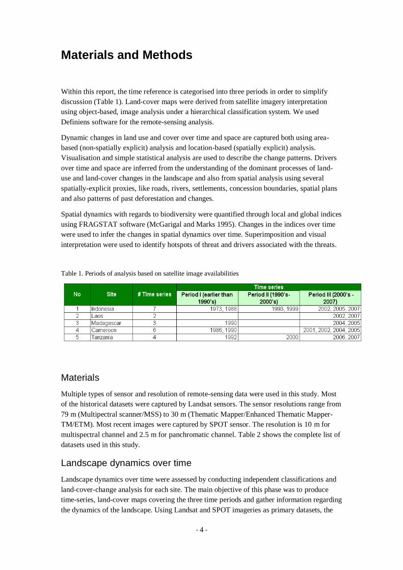
Within this report, the time reference is categorised into three periods in order to simplify
discussion (Table 1). Land-cover maps were derived from satellite imagery interpretation
using object-based, image analysis under a hierarchical classification system. We used
Definiens software for the remote-sensing analysis.
Dynamic changes in land use and cover over time and space are captured both using area-
based (non-spatially explicit) analysis and location-based (spatially explicit) analysis.
Visualisation and simple statistical analysis are used to describe the change patterns. Drivers
over time and space are inferred from the understanding of the dominant processes of land-
use and land-cover changes in the landscape and also from spatial analysis using several
spatially-explicit proxies, like roads, rivers, settlements, concession boundaries, spatial plans
and also patterns of past deforestation and changes.
Spatial dynamics with regards to biodiversity were quantified through local and global indices
using FRAGSTAT software (McGarigal and Marks 1995). Changes in the indices over time
were used to infer the changes in spatial dynamics over time. Superimposition and visual
interpretation were used to identify hotspots of threat and drivers associated with the threats.
Table 1. Periods of analysis based on satellite image availabilities
Materials
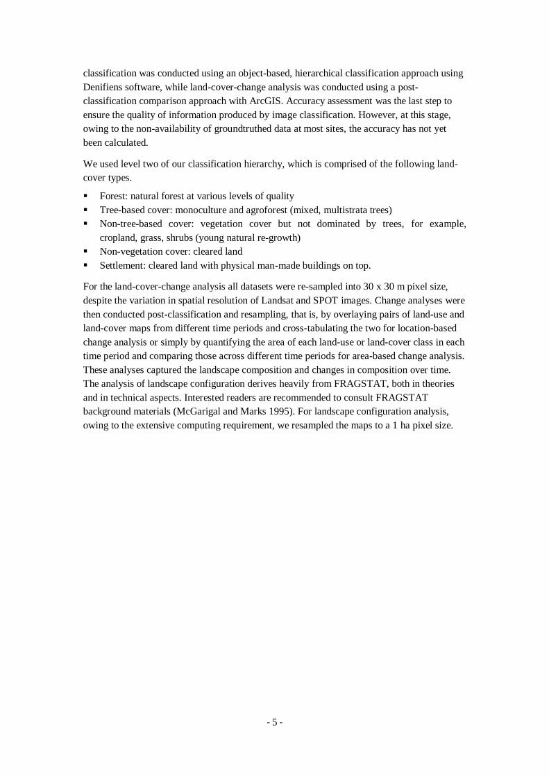
Multiple types of sensor and resolution of remote-sensing data were used in this study. Most
of the historical datasets were captured by Landsat sensors. The sensor resolutions range from
79 m (Multipectral scanner/MSS) to 30 m (Thematic Mapper/Enhanced Thematic Mapper-
TM/ETM). Most recent images were captured by SPOT sensor. The resolution is 10 m for
multispectral channel and 2.5 m for panchromatic channel. Table 2 shows the complete list of
datasets used in this study.
Landscape dynamics over time
Landscape dynamics over time were assessed by conducting independent classifications and
land-cover-change analysis for each site. The main objective of this phase was to produce
time-series, land-cover maps covering the three time periods and gather information regarding
the dynamics of the landscape. Using Landsat and SPOT imageries as primary datasets, the
- 5 -
classification was conducted using an object-based, hierarchical classification approach using
Denifiens software, while land-cover-change analysis was conducted using a post-
classification comparison approach with ArcGIS. Accuracy assessment was the last step to
ensure the quality of information produced by image classification. However, at this stage,
owing to the non-availability of groundtruthed data at most sites, the accuracy has not yet
been calculated.
We used level two of our classification hierarchy, which is comprised of the following land-
cover types.
Forest: natural forest at various levels of quality
Tree-based cover: monoculture and agroforest (mixed, multistrata trees)
Non-tree-based cover: vegetation cover but not dominated by trees, for example,
cropland, grass, shrubs (young natural re-growth)
Non-vegetation cover: cleared land
Settlement: cleared land with physical man-made buildings on top.
For the land-cover-change analysis all datasets were re-sampled into 30 x 30 m pixel size,
despite the variation in spatial resolution of Landsat and SPOT images. Change analyses were
then conducted post-classification and resampling, that is, by overlaying pairs of land-use and
land-cover maps from different time periods and cross-tabulating the two for location-based
change analysis or simply by quantifying the area of each land-use or land-cover class in each
time period and comparing those across different time periods for area-based change analysis.
These analyses captured the landscape composition and changes in composition over time.
The analysis of landscape configuration derives heavily from FRAGSTAT, both in theories
and in technical aspects. Interested readers are recommended to consult FRAGSTAT
background materials (McGarigal and Marks 1995). For landscape configuration analysis,
owing to the extensive computing requirement, we resampled the maps to a 1 ha pixel size.
- 6 -
Table 2. List of materials used for this interim report (additional images will be used in the near future,
especially for Lao PDR and Madagascar)
No Site name Country Time series Sensor Resolution
1 Bungo Indonesia 1973 MSS 79m
1988 TM 30 m
1993 TM 30 m
1999 TM 30 m
2002 ETM 30 m
2005 ETM-SLC off 30 m
2006 SPOT 5 10 m/2.5 m
2 Viengkham Laos 2005 ETM-SLC off 30 m
2007 SPOT 5 10 m/2.5 m
3 Manompana Madagascar 1990 ETM 30 m
2005 ETM-SLC off 30 m
2007 SPOT 5 10 m/2.5 m
4 Takamanda-Mone Cameroon 1986 TM 30 m
1990 TM 30 m
2001 ETM 30 m
2002 ETM 30 m
2004 SPOT 5 10 m/2.5 m
2005 ETM-SLC off 30 m
5 East Usambara Tanzania 1992 TM 30 m
2000 TM 30 m
2006 ETM-SLC off 30 m
2007 SPOT 5 10 m/2.5 m
We used FRAGSTAT software to calculate some landscape and class indices for pattern
quantification. We selected a few indices only, among a large number made available by
FRAGSTAT, based on the uniqueness of information expressed by the indices, since many
indices highly correlate to each other, and on their relevance to ecological processes. In this
interim report, we will only present a few of the indices. We will cover both structural and
functional indices and run the analysis both at the global and local (sub-landscape) levels.
Global-level indices are calculated for the entire landscape while the local level indices are
calculated based on a specified window size.
Modified Simpson‟s diversity and evenness indices are used to capture landscape composition
while total core area, aggregation index and connectivity index measure landscape
configuration, with the connectivity index reflecting the ecological functions of connecting
one habitat to another from species‟ perspectives.

- 7 -
Modified Simpson‟s diversity index measures the proportional abundance of each patch
type. When the landscape contains only one patch (that is, no diversity), the index is equal
to 0. It increases as the number of different patch types increases and the proportional
distribution of area among patch types becomes more equitable.
Modified Simpson‟s evenness index measures the proportional abundance of each patch
divided by the total number of patch types. It is equal to 0 when h (that is, no diversity)
and equals 1 when distribution of area among patch types is perfectly even (that is,
proportional abundances are the same).
Total core area is the sum of the core areas of each patch, which is calculated based on
specified depth-of-edge distance(s) from the patch perimeters. Total core area considers
the reduction in the area by the encroachment from the edge at a specified depth; as patch
shapes are more complicated and patch perimeters are longer, the differences between
total area and total core area are larger.
Aggregation index measures the likelihood of patches of corresponding classes being
adjacent to each other.
Connectivity index measures the functional joining between all patches of the
corresponding patch type based on defined similarity.
Further description of the indices can be found in the FRAGSTAT manual and user guides.
These indices are calculated at the global (across the entire dataset) landscape; one landscape
has one value of these indices attached to it under the same set of parameters. Changes in
landscape over time and differences in patterns across landscapes of different places can be
studied by comparing these values. Some of these indices are normalised so that they are not
sensitive to sizes of landscapes to allow direct comparison of landscapes of varying extent.
We use the same parameters across landscapes at the five study sites.
Edge depth
Land-cover type Forest Tree-based Non-tree-based Non-vegetation
Forest 0 200 100 100
Tree-based 0 0 200 100
Non-tree-based 0 0 0 100
Non-vegetation 0 0 0 0
Similarity
Land-cover type Forest Tree-based Non-tree-based Non-vegetation
Forest 1 0.8 0.2 0
Tree-based 0.8 1 0.3 0
Non-tree-based 0 0.3 1 0.1
Non-vegetation 0.3 0 0.1 1
- 8 -
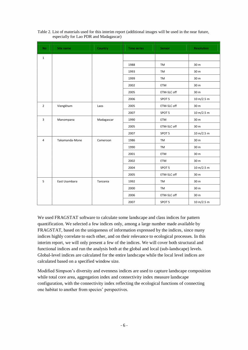
Edge weight
Land-cover type Forest Tree-based Non-tree-based Non-vegetation
Forest 0 0.3 0.8 1
Tree-based 0.3 0 0.5 0.8
Non-tree-based 0.8 0.5 0 0.3
Non-vegetation 1 0.8 0.3 0
The edge depth parameter assumes that the encroachment on forest by tree-based vegetation
is 200 m while non-tree and non-vegetation are half of that of tree-based. The similarity
parameter assumes that tree-based vegetation is 80% similar to forest, while non-tree is only
20%. The edge weight assumes dissimilarity of tree-based and forest is 30% while non-tree is
80%. These parameters are at this moment solely based on expert judgment and will be
evaluated against field data later.
Landscape dynamics over space
The landscape indices above are derived from the assumption that only the overall patterns at
landscape level matter and variations within a landscape can be ignored. However, for a large
enough landscape and for small- body species or species that only forage or disperse
narrowly, local variations in sub-landscape level are at least as important and therefore it is
crucial to quantify patterns locally over a landscape space. The direct application might be
hotspot and threat location identification for land-use planning.
We use a circular moving window of radius 1000 m to define a sub-landscape of such size
and calculate several indices that reflect composition and configuration within the sub-
landscape. These computations require extensive processing power, especially for large
landscape, high resolution maps and a large number of classes or land-cover types. Re-
sampling from the original resolution to a coarser resolution is needed for these computations
owing to hardware limitations. The parameters we use for calculating local composition and
configuration indices are the same as those for global ones. The outputs are presented as a
series of maps; each pixel represents the value of the indices of the sub-landscape, calculated
within a circle of 1 km radius.
Landscape dynamics over time and space
In this report, the comparison across time and space and among landscapes will only be
presented through the series of maps. The output at this stage will be useful for the practical
uses of focus group discussion and visioning and as the basis for further exploration using
different sets of parameters. Further, these results will be analysed and summarised under the
what-if scenario and projections of land-use and land-cover changes.
- 9 -
Results and discussion
Landscape dynamics over time
This section describes the current land cover, temporal changes, location changes and drivers
in each landscape and then discusses them across landscapes. We also present descriptions of
global landscape composition and configuration of landscapes over time.
Indonesia (Bungo)
Topography and current land cover
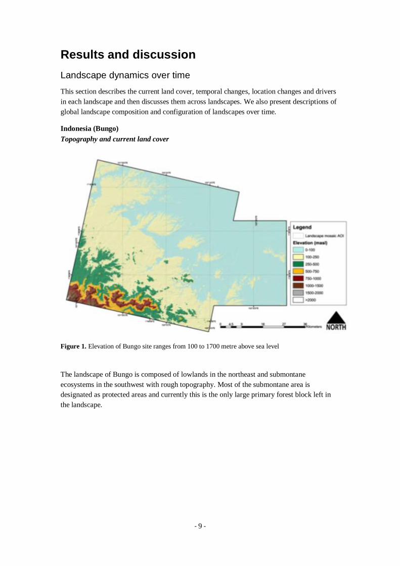
Figure 1. Elevation of Bungo site ranges from 100 to 1700 metre above sea level
The landscape of Bungo is composed of lowlands in the northeast and submontane
ecosystems in the southwest with rough topography. Most of the submontane area is
designated as protected areas and currently this is the only large primary forest block left in
the landscape.

- 10 -
Figure 2. (a) Land-cover map of Bungo site in 2007 (interpreted from SPOT 2007); (b) Landscape
composition in 2007
In 2007, two-thirds of the Bungo landscape was dominated by the tree-based land-cover type;
only 16% of the area was covered by natural forest. Most of the natural forest cover exist as
primary forest blocks of substantial sizes with complex shapes, surviving only at higher
altitudes, surrounded by some small disconnected patches of primary, but degraded forest.
Other even smaller forest patches still exist along the lower Batang Hari River as riparian
forest.

- 11 -
Temporal pattern
Figure 3. Time series, land-cover composition of Bungo site
Natural forest cover declined in period I, especially between 1973 to 1988, but tree-based
land cover took over and has become the dominant land cover since then (Figure 3). This tree-
based land cover continued to increase until 1999 (period II), when it stabilised. During
period III, changes were within the tree-based land cover class; a large proportion of
agroforest (rubber multistrata) was converted to more intensively managed tree-based
systems, such as rubber monoculture, oil palm and, very recently, to Acacia mangium. In this
case, the image interpretation needs a finer classification scheme to differentiate further the
types of the tree-based systems, especially when the focus is on biodiversity. At the time of
writing this interim report, we had not yet finalised the image interpretation using the finest
classification scheme. The finer classification process is scheduled to take place after the
fieldwork is conducted in order to obtain more groundtruthed data.

- 12 -
(a)
(b)
(c)
Figure 4. Patterns of changes in three study periods: (a) Period I (1973–1993); (b) Period II (1993–2002); and (c) Period III (2002–2007). Darker colors indicate larger annual changes in proportion
The pattern of changes during the three periods follows closely the forest transition theory.
The earlier stage was dominated by loss of forest and biomass, in which most forests were
converted to tree-based systems in period II (Figure 4). In Bungo, this period was also marked
by increases in population and settlement area. There were new areas developed under the
transmigration programs, both from surrounding areas and also from Java. The third period
was marked with conversion of established tree-based systems to non-tree-based systems and
vegetation, which suggests either the transition to more intensified cropland and settlement or
transition to more intensified tree-based systems, mostly monoculture rather than mixed tree,
especially oil palm and rubber.
Location of changes
During the earliest period, deforestation occurred from the northern to the southern part of the
district and, while this continues, the second period experiences further changes from the east
toward the west (Figure 5 and 6). The common characteristics have been that forest loss
started from lowland areas by timber harvesting that provided higher economic benefits,
followed by clearing and conversion to either timber plantations, estate plantations, rubber
agroforests, cropland or settlements. The most recent deforestation occurred on the edges of
the major primary forest block mostly found in higher altitudes only.
- 13 -
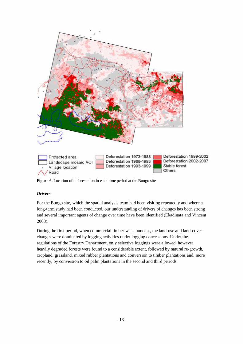
Figure 6. Location of deforestation in each time period at the Bungo site
Drivers
For the Bungo site, which the spatial analysis team had been visiting repeatedly and where a
long-term study had been conducted, our understanding of drivers of changes has been strong
and several important agents of change over time have been identified (Ekadinata and Vincent
2008).
During the first period, when commercial timber was abundant, the land-use and land-cover
changes were dominated by logging activities under logging concessions. Under the
regulations of the Forestry Department, only selective loggings were allowed, however,
heavily degraded forests were found to a considerable extent, followed by natural re-growth,
cropland, grassland, mixed rubber plantations and conversion to timber plantations and, more
recently, by conversion to oil palm plantations in the second and third periods.

- 14 -
1973 1988 1993 1999
2002 2005 2007
Figure 5. Time series, land-cover maps of Bungo site

- 15 -
On smallholder-managed land, during the first period the dominant land uses were rice fields,
croplands under shifting cultivation systems, rubber agroforests and some rubber monoculture
(intensive rubber). During the first period, there was not much interaction between farmers and
the large-scale drivers in terms of land cover and use. In the second period, farmers started to
convert their rubber agroforest to more intensively managed rubber gardens. Also some farmers
started to plant oil palm a result of interaction with larger-scale agents.
The third period up to now is heavily dominated by conversion to oil palm and, to a lesser degree,
timber plantations mostly for fibre, both under large- and small-scale concessions with out-
grower schemes. This latest trend is driven by global demand for oil palm and rubber and
regional demand for raw materials for pulp and paper owing to depletion of natural forest and
improved law enforcement. Following the „anarchy‟ period caused by the euphoria of the
enactment of the decentralisation law, which resulted in lack of clarity and uncertainty over land
tenure (aspects of which have not been resolved up to now), land grabbing by farmers was quite
prevalent. A discussion of the overall forest and landscape governance issues of Bungo can be
found in Martini et al. (2010).
The transmigration program, facilitated by the government, has also been active. This involved
people migrating from the surrounding area, known as local transmigration, and from Java.
Associated with this program was the establishment of cropland and tree-based systems from
forest and shrubs.
Most recently, activities and permits for coal mining have been increasing sharply. This has
become a new driver of land-use and land-cover changes in the area. Despite this, Lubuk
Beringin, one of the villages within the Bungo landscape, has been awarded a Hutan Desa
(Village Forest) permit, the first in Indonesia (Akiefnawati et al. 2010).

- 16 -
Figure 7. Forest loss (in hectare) in each time series by elevation class
Access (river or road network)
In the past, people depended on rivers for their transportation network but, lately, the road
network has become well established; most settlements in Bungo are now connected to larger
townships by road. The location of deforestation in Bungo correlates strongly with the existence
of roads, like everywhere else in the tropics.
Protected area
Kerinci Seblat National Park covers the higher altitude areas in Bungo and is part of the Bukit
Barisan mountain range. Up to now, the forest area of the national park in Bungo has been well
conserved as part of the major block of primary forest remaining in the landscape. However, past
trends show active encroachment from the forest edges, threatening the buffer area of the national
park with forest degradation, if not deforestation.

- 17 -
Lao PDR (Viengkham)
Topography, current land cover and description
Figure 8. Elevation of Viengkham site ranges from 400 to 2200 metre above sea level
The landscape of Viengkham is dominated by a montane ecosystem with rough topography,
especially in the eastern half of the area and some parts of the northwest (Figure 8). Among the
five sites of the project, Lao PDR is highest and roughest in terms of topography.
- 18 -
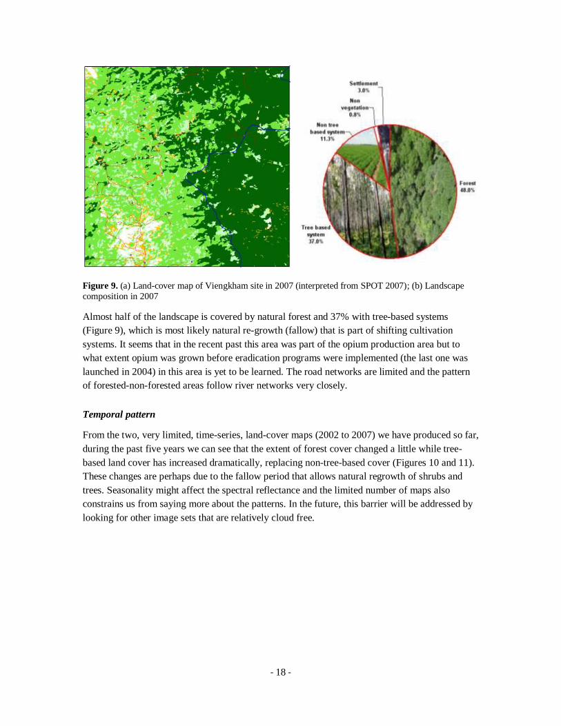
Figure 9. (a) Land-cover map of Viengkham site in 2007 (interpreted from SPOT 2007); (b) Landscape
composition in 2007
Almost half of the landscape is covered by natural forest and 37% with tree-based systems
(Figure 9), which is most likely natural re-growth (fallow) that is part of shifting cultivation
systems. It seems that in the recent past this area was part of the opium production area but to
what extent opium was grown before eradication programs were implemented (the last one was
launched in 2004) in this area is yet to be learned. The road networks are limited and the pattern
of forested-non-forested areas follow river networks very closely.
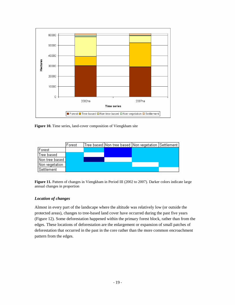
Temporal pattern
From the two, very limited, time-series, land-cover maps (2002 to 2007) we have produced so far,
during the past five years we can see that the extent of forest cover changed a little while tree-
based land cover has increased dramatically, replacing non-tree-based cover (Figures 10 and 11).
These changes are perhaps due to the fallow period that allows natural regrowth of shrubs and
trees. Seasonality might affect the spectral reflectance and the limited number of maps also
constrains us from saying more about the patterns. In the future, this barrier will be addressed by
looking for other image sets that are relatively cloud free.
- 19 -
Figure 10. Time series, land-cover composition of Viengkham site
Figure 11. Pattern of changes in Viengkham in Period III (2002 to 2007). Darker colors indicate large
annual changes in proportion
Location of changes
Almost in every part of the landscape where the altitude was relatively low (or outside the
protected areas), changes to tree-based land cover have occurred during the past five years
(Figure 12). Some deforestation happened within the primary forest block, rather than from the
edges. These locations of deforestation are the enlargement or expansion of small patches of
deforestation that occurred in the past in the core rather than the more common encroachment
pattern from the edges.

- 20 -
Location of changes
. 2002 2007
Figure 12. Time series, land-cover maps of Viengkham site

- 21 -
Figure 13. Location of deforestation at the Viengkham site
Drivers
Agents
Deforestation has occurred in the protected area. Dense forests have become scarce in agricultural
landscapes with relatively high accessibility and remain only in less accessible areas. The typical
landscape consists of patches of different gradients of vegetation from degraded forest to
grassland and is a consequence of human impact (slash and burn cultivation for upland rice, other
farming systems, cash crop plantation, possibly effects of war etc).
The main income sources are livestock (pigs, cattle, chicken etc), followed by the collection of
non-timber forest products (bamboos, grasses for brooms, mushrooms). Teak cultivation is
limited owing to land tenure issues and availability. Technical limitations are also marked, for
example, in the case of eaglewood. Rubber planting is of interest to local people but there are
very few trials, mostly owing to the rough terrain and difficult market access. Population density
of this landscape is very low. Shifting cultivation is the dominant land-use system in the area. In
2004, the government enacted a policy to reduce the area of shifting cultivation by shortening the
fallow period to three years only, as extensive shifting cultivation is believed to be the single
most important reason for deforestation and degradation.

- 22 -
Topography
Figure 14 shows that most forest loss happened in the lower altitudes, however, since we only
have two time periods we cannot compare the pattern of forest loss with regard to topography
during different periods. In the highest elevation area (> 1500 m), forest loss was quite marked
compared to the intermediate elevation class (1000–1500 m), perhaps induced by new road
development or other external drivers.
Figure 14. Forest loss (in hectare) by elevation class
Access
Road access to the forests from Viengkham is limited, but some tracks are passable by motorbike
during the dry season, otherwise farmers need to walk or build semi-permanent huts in the
forested areas to extract non-timber forest products or grow upland rice. Some major rivers are
still functioning as transportation networks but in most upland areas road is the main, but limited,
network.
Protected area
Phou Loei National Biodiversity Conservation Area covers 150 000 ha (category VI according to
the United Nations Environment Programme‟s World Conservation Monitoring Centre). It was
established in 1993 and is located in Phonxay and Viengkham districts. It is a „managed resource
protected area‟, where the conservation objective is sustainable use of its natural ecosystems.
- 23 -
Madagascar (Manompana)
Topography, current land cover and description
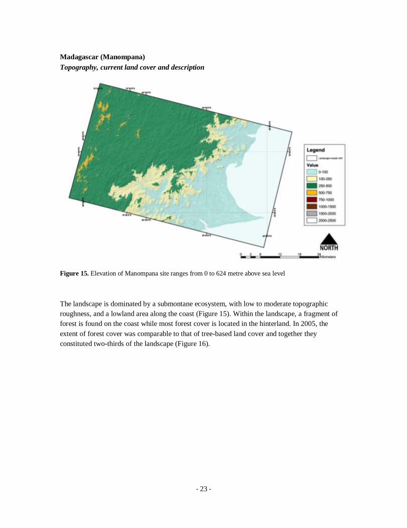
Figure 15. Elevation of Manompana site ranges from 0 to 624 metre above sea level
The landscape is dominated by a submontane ecosystem, with low to moderate topographic
roughness, and a lowland area along the coast (Figure 15). Within the landscape, a fragment of
forest is found on the coast while most forest cover is located in the hinterland. In 2005, the
extent of forest cover was comparable to that of tree-based land cover and together they
constituted two-thirds of the landscape (Figure 16).

- 24 -
Figure 16. (a) Land-cover map of Manompana site in 2005 (interpreted from SPOT 2005); (b) Landscape
composition in 2005
Temporal pattern
Figure 17. Time series, land-cover composition of Manompana site

- 25 -
A large amount of deforestation took place in period II and there has been little forest loss since
(note that the observation period is only one year). Both tree-based and non-tree-based land cover
increased as replacements to forest. It seems that while the extent of tree-based and non-tree
based cover remains stable in the landscape (Figure 17), the location is changing (Figure 18),
which indicates that shifting cultivation is actively taking place.
(a)
(b)
Figure 18. (a) Pattern of changes in Manompana in Period II (1990 to 2004); and (b) Period III (2004 to
2005). Darker colors indicate larger annual changes in proportion

- 26 -
Location of changes
Figure 19. Time series, land-cover maps of Manompana site
1990
2005
2004
- 27 -
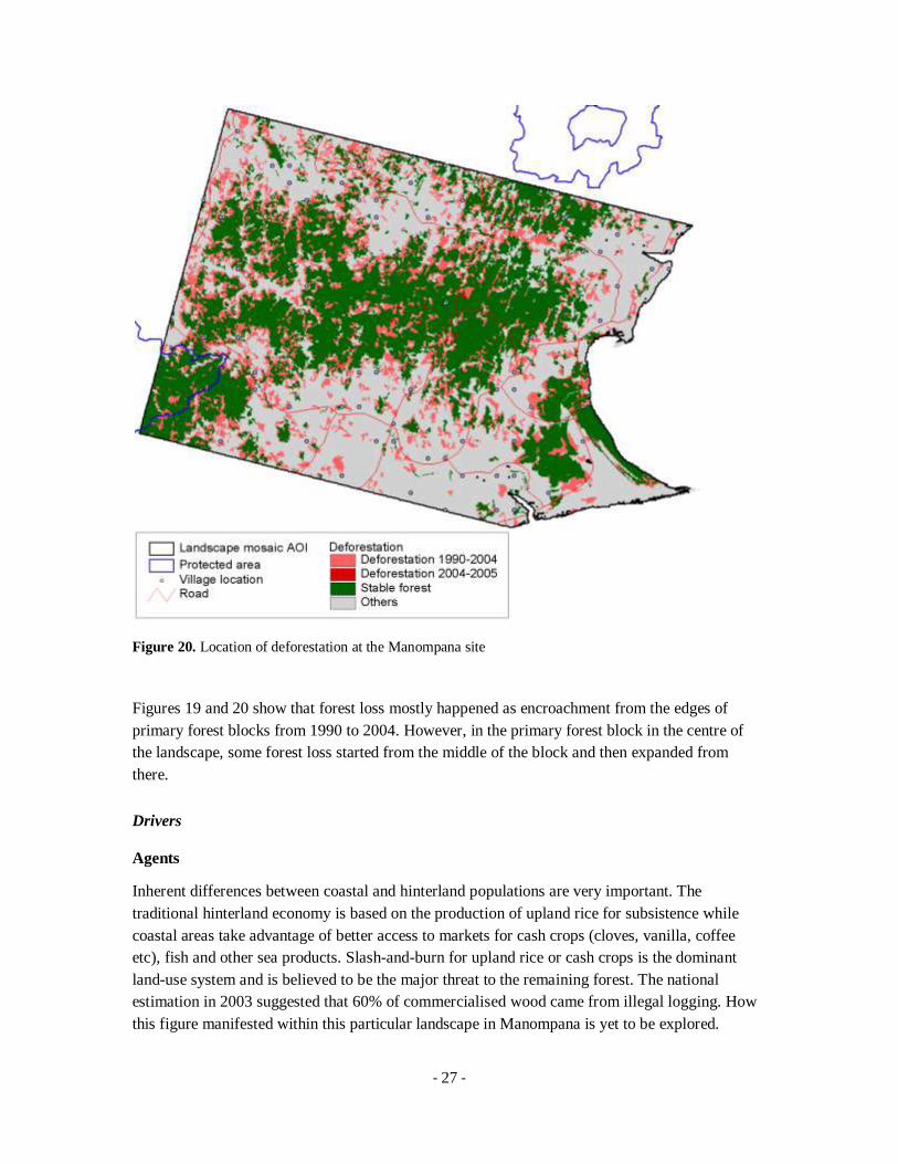
Figure 20. Location of deforestation at the Manompana site
Figures 19 and 20 show that forest loss mostly happened as encroachment from the edges of
primary forest blocks from 1990 to 2004. However, in the primary forest block in the centre of
the landscape, some forest loss started from the middle of the block and then expanded from
there.
Drivers
Agents
Inherent differences between coastal and hinterland populations are very important. The
traditional hinterland economy is based on the production of upland rice for subsistence while
coastal areas take advantage of better access to markets for cash crops (cloves, vanilla, coffee
etc), fish and other sea products. Slash-and-burn for upland rice or cash crops is the dominant
land-use system and is believed to be the major threat to the remaining forest. The national
estimation in 2003 suggested that 60% of commercialised wood came from illegal logging. How
this figure manifested within this particular landscape in Manompana is yet to be explored.

- 28 -
The fallow system is the dominant land-use system in Manompana. Most deforestation is
believed to be driven by this type of agricultural expansion. Around villages, home gardens of
banana, papaya and other fruit trees are commonly managed in mixed agroforestry systems while
commodities like coffee, cloves and vanilla are planted as monoculture (Pfund et al. 2010).
Topography
Figure 21 shows that most of the forest loss in each of the elevation classes is comparable to the
existing forest, which suggests that there is no particular tendency for forest loss to be associated
with topography.
Figure 21. Forest loss (in hectare) in each period by elevation class
Access
Even though the road network is very limited, the population seems to be well distributed across
the landscape, including in the big forest blocks. Some river networks are functioning as
transportation but generally people use walking paths to travel from place to place.
- 29 -
Cameroon (Takamanda-Mone)
Topography, current land cover and description
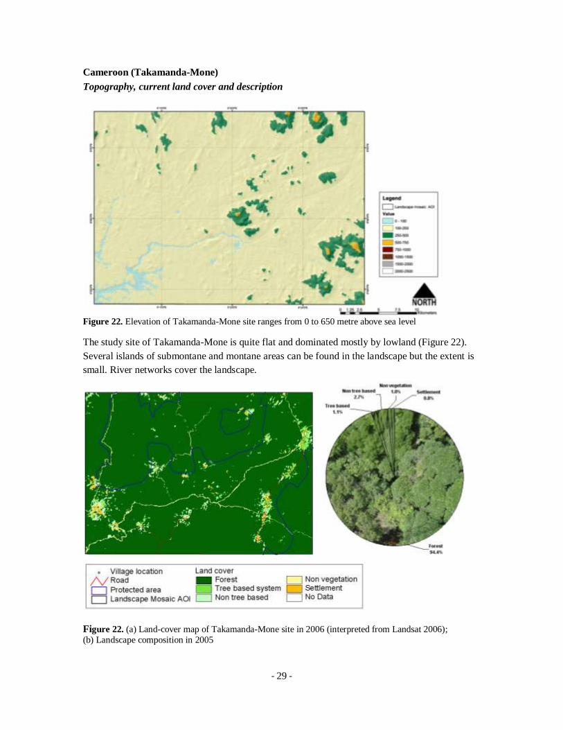
Figure 22. Elevation of Takamanda-Mone site ranges from 0 to 650 metre above sea level
The study site of Takamanda-Mone is quite flat and dominated mostly by lowland (Figure 22).
Several islands of submontane and montane areas can be found in the landscape but the extent is
small. River networks cover the landscape.
Figure 22. (a) Land-cover map of Takamanda-Mone site in 2006 (interpreted from Landsat 2006);
(b) Landscape composition in 2005

- 30 -
In 2006, Takamanda-Mone was highly dominated by forest (94.4%), with some settlements found
along the rivers and surrounded by some other land cover (Figure 22). Most of the areas are under
protected status.
Temporal pattern
Figure 23. Time series, land-cover composition of Takamanda-Mone site
Within the time series, forest loss has been relatively small compared to other sites. The increase
of non-tree-based cover is quite marked in the most recent years (Figure 23). Another pattern to
note is the increase of area of settlement (Figure 24). This perhaps indicates either population
increases (due to in-migration) or resettlement. Interchange from tree-based to non-tree-based
cover and vice versa is also high.

- 31 -
(a)
(b)
(c)
Figure 24. Pattern of changes in Takamanda-Mone for three study periods: (a) Period I (1986–1990);
(b) Period II (1990–2000); and (c) Period III (2000–2005). Darker colors indicate larger annual changes in proportion

- 32 -
Location of changes
1986 1990 2001
2002 2004 2005
Figure 25. Time-series, land-cover maps of Takamanda-Mone site

- 33 -
Figure 25 shows that most of the deforestation patterns follow the river and road networks. Over
time the settlements that started earlier expanded further into the forest. This indicates that
smallholder farmers are the dominant agent in the landscape.
Figure 26. Location of deforestation at Takamanda-Mone site

- 34 -
Drivers
Topography
Figure 27. Forest loss over time by elevation class
Whilst the earlier period showed comparable forest loss in the lower and moderate elevation
classes in relation to the existing forest, the most recent forest loss revealed a new pattern: forest
loss at elevations of 100–250 m is higher compared to those in the lower altitudes (Figure 27).
Population growth, either naturally or by resettlement, in tandem with new road construction can
be the explanation of this pattern.
In this landscape, logging is active, but since forests are not differentiated in terms of density, that
is, between dense and degraded or logged-over forest, selected loggings are not detectable.
Fallows are not identified as part of a cultivation cycle. Cultivation of cocoa, mixed with banana
and plantains, along the roads have increased recently owing to market access. Small-scale oil
palm plantations have been introduced and developed in the secondary forests as well as tree
plantings such as bush mango (Irvingia wombolo), bitter cola (Garcinia cola), and njansang
(Ricinodendron heudelotii) which provide substantial income to farmers (Pfund et al. 2010).

- 35 -
Tanzania (East Usambara)
Topography, current land cover and description
Figure 28. Elevation of East Usambara site ranges from 100 to 1500 metre above sea level
The landscape of East Usambara is the second highest and roughest in terms of topography
among the five sites. Topographically, the landscape consists of one big island of montane
ecosystems and three other smaller islands; two of them are disconnected from the biggest island
(Figure 28).
In 2007, three-quarters of the landscape was covered by forest and tree-based systems of
comparable proportion. Compared to the other sites, forest cover in East Usambara landscapes is
the most scattered and fragmented. The shape of forest patches is also complex with long edges
compared to their areas. Forest patches are found mostly in montane and submontane areas and to
a lesser extent in the lowlands.

- 36 -
Figure 29. (a) Land-cover map of East Usambara site in 2007 (interpreted from SPOT 2007);
(b) Landscape composition in 2007
Temporal pattern
Forest continues to decline over time. The proportion of tree-based to non-tree-based cover
interchanges over time, whilst settlement areas show steady increases in size. Most recently, tree-
based cover dominates the landscape.
- 37 -
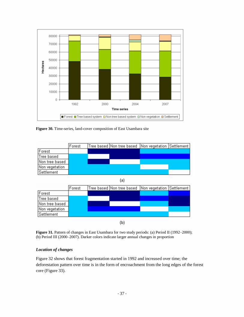
Figure 30. Time-series, land-cover composition of East Usambara site
(a)
(b)
Figure 31. Pattern of changes in East Usambara for two study periods: (a) Period II (1992–2000);
(b) Period III (2000–2007). Darker colors indicate larger annual changes in proportion
Location of changes
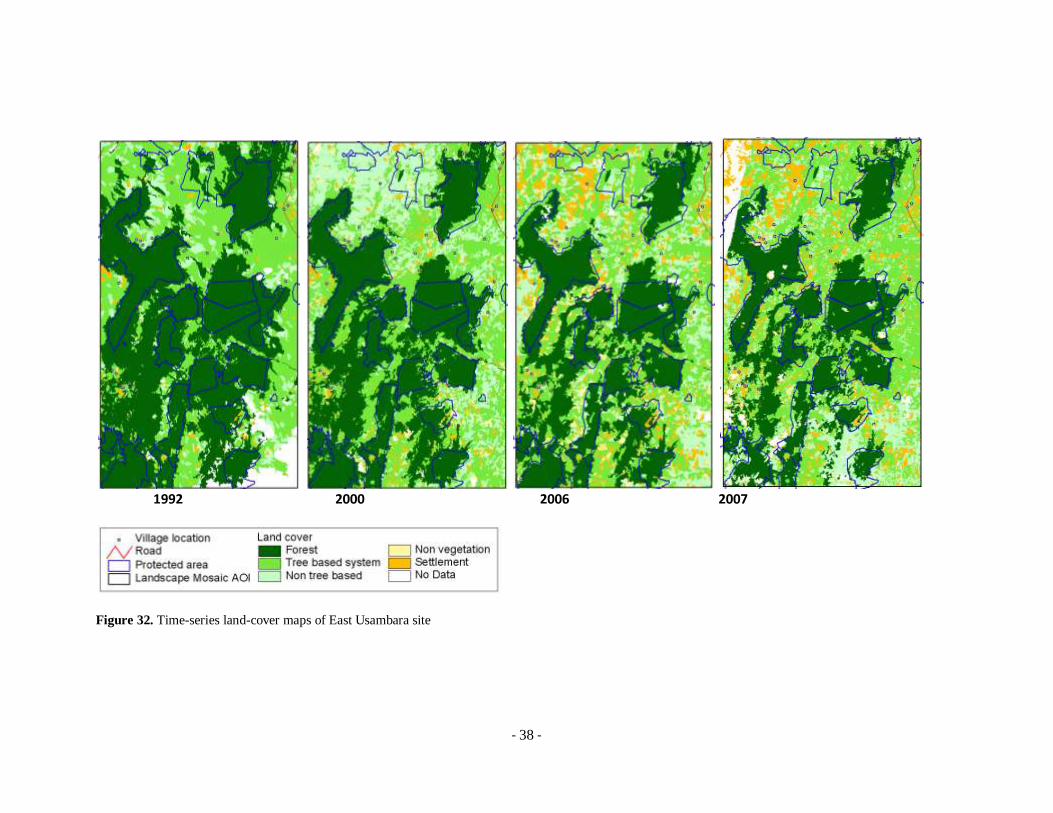
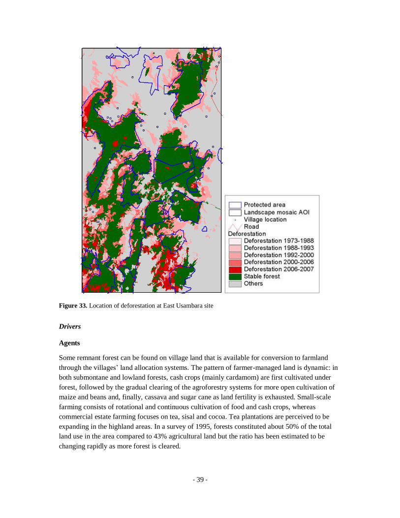
Figure 32 shows that forest fragmentation started in 1992 and increased over time; the
deforestation pattern over time is in the form of encroachment from the long edges of the forest
core (Figure 33).
- 38 -
1992 2000 2006 2007
Figure 32. Time-series land-cover maps of East Usambara site
- 39 -
Figure 33. Location of deforestation at East Usambara site
Drivers
Agents
Some remnant forest can be found on village land that is available for conversion to farmland
through the villages‟ land allocation systems. The pattern of farmer-managed land is dynamic: in
both submontane and lowland forests, cash crops (mainly cardamom) are first cultivated under
forest, followed by the gradual clearing of the agroforestry systems for more open cultivation of
maize and beans and, finally, cassava and sugar cane as land fertility is exhausted. Small-scale
farming consists of rotational and continuous cultivation of food and cash crops, whereas
commercial estate farming focuses on tea, sisal and cocoa. Tea plantations are perceived to be
expanding in the highland areas. In a survey of 1995, forests constituted about 50% of the total
land use in the area compared to 43% agricultural land but the ratio has been estimated to be
changing rapidly as more forest is cleared.
- 40 -
During the past decades, other groups have migrated into the area, attracted by the favourable
climatic conditions and job opportunities in the tea plantations. The population is rapidly growing
at an annual rate of 2.2% (2001). The majority of the population belongs to the poor segment of
smallholder farmers and tea estate workers.
Outside the protected areas, forest loss continues rapidly for agricultural conversion owing to
increasing population pressure. People see the remaining forest as their future agricultural land
and resist government efforts to gazette new protected areas to increase connectivity between
remnant forest patches. Some advance has been made in the establishment of community
managed Village Forest Reserves, since people are now increasingly dependent on the remaining
forest in reserves for medicinal plants, fuel wood and building materials, as well as services such
as a regular water supply. Fire is a major threat to forests both outside and inside the reserves
owing to burning of adjacent fields. Since 2004, a new threat to the forests and water reserves has
emerged in the form of a considerable increase in small-scale mining. Also the impact of a
growing industrial demand for firewood (for tea curing) is becoming more significant and new
forest areas are cleared for fuel wood without a strategy for regeneration.
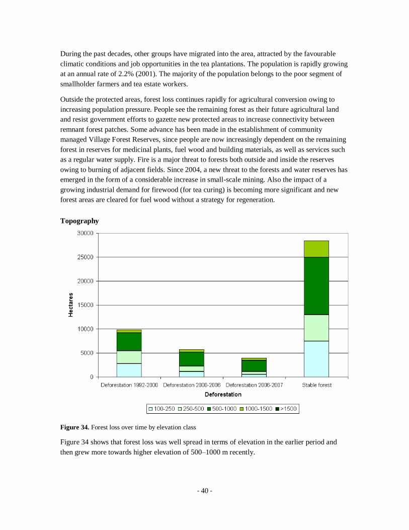
Topography
Figure 34. Forest loss over time by elevation class
Figure 34 shows that forest loss was well spread in terms of elevation in the earlier period and
then grew more towards higher elevation of 500–1000 m recently.
Top Related
Copyright © 2022 FDOKUMEN

