Download - Investigation of a System Identification Methodology in the Context of the ASCE Benchmark Problem

Investigation of a System Identification Methodology in

the Context of the ASCE Benchmark Problem

Hilmi Lus∗, Raimondo Betti †, Jun Yu‡and Maurizio De Angelis§

Abstract

This article briefly presents the theory for a system identification and damage detection algo-

rithm for linear systems, and discusses the effectiveness of such a methodology in the context of

a benchmark problem that was proposed by the ASCE Task Group in Health Monitoring. The

proposed approach has two well defined phases: (i) identification of a state space model using

OKID, ERA, and a non-linear optimization approach based on sequential quadratic programming

techniques, and (ii) identification of the second-order dynamic model parameters from the realized

state space model. Structural changes (damage) are characterized by investigating the changes

in the second-order parameters of the “reference” and “damaged” models. An extensive numeri-

cal analysis, along with the underlying theory, is presented in order to assess the advantages and

disadvantages of the proposed identification methodology.

∗Asst. Prof., Dept. of Civil Eng., Bogazici University, Bebek 80815 Istanbul, Turkey†Assoc. Prof., Dept. of Civil Eng. and Eng. Mechanics, Columbia University, New York, NY, 10027‡Grad. Stud., Dept. of Civil Eng. and Eng. Mechanics, Columbia University, New York, NY, 10027§Asst. Prof., Dip. Ing. Strutt. e Geotecnica, Univ. di Roma “La Sapienza”, Rome, Italy

1

Lus, Betti, Yu, and De Angelis ASCE J. Eng. Mech, Benchmark Issue

1 Introduction

Recently, in an effort to bring together researchers working in the field of system identification and

health monitoring, and for verification of various damage detection algorithms, a benchmark problem

was proposed by the ASCE Task Group in Health Monitoring. This benchmark problem consists of

two phases: in the first one, the system identification and damage detection analysis is conducted

on simulated numerical models of structural systems, and in the second phase, the investigation is

extended to include an experimental stage. This article is a brief summary of some investigations

conducted during the first phase of such a benchmark problem.

Here we discuss the application of a two-step methodology that consists of, first, finding a first-

order minimal state space realization of the system using only input-output measurements, and then,

extracting the physical parameters (i.e. the mass, damping, and stiffness matrices) of the underlying

second-order system. Initially, it is assumed that the structure (model) under investigation is sub-

jected to measured dynamic excitations (inputs), and that concurrently measurements, in the form of

either displacements, velocities, and/or accelerations, are obtained at various locations on the structure

(outputs). These input and output measurements are then used in the Observer/Kalman filter IDen-

tification (OKID) algorithm (Juang et al., 1993; Lus et al., 1999) to identify the Markov parameters

of the system, which are in turn used in the Eigensystem Realization Algorithm (ERA) (Juang and

Pappa, 1985) to realize the discrete time first-order system matrices. This initial state space model is

further refined by minimizing the output error between the measured and predicted response using a

non-linear optimization approach based on sequential quadratic programming techniques (Lus et al.,

2002; Lus, 2001). Once the final form of the state space model is obtained, the physical parameters

of the second-order (finite element) model are retrieved from this state space model following the ap-

proach presented in Lus (2001) and DeAngelis et al. (2002). Any structural changes (“damage”) are

then evaluated qualitatively and quantitatively by inspecting the variations in the physical parameters

of the reference and the damaged models.

At this juncture, it should be mentioned that the literature on damage detection is vast and growing,

2

https://www.researchgate.net/publication/23867444_Identification_of_Observer_KalmanFilter_Markov_parameters_-_theory_and_experiments?el=1_x_8&enrichId=rgreq-60ac8e84-8c38-4ce9-947a-cfe935db0c5d&enrichSource=Y292ZXJQYWdlOzI0NTI4NjQ0MDtBUzoxMzIyMzAxNDM4MTE1ODVAMTQwODUzNzUzMTU4Nw==

https://www.researchgate.net/publication/260052496_Extracting_Physical_Parameters_of_Mechanical_Models_From_Identified_State-Space_Representations?el=1_x_8&enrichId=rgreq-60ac8e84-8c38-4ce9-947a-cfe935db0c5d&enrichSource=Y292ZXJQYWdlOzI0NTI4NjQ0MDtBUzoxMzIyMzAxNDM4MTE1ODVAMTQwODUzNzUzMTU4Nw==


and that therefore a complete review of the subject is beyond the scope of this study. Some of the

noteworthy efforts in this area are the works by Agbabian et al. (1991), Friswell et al. (1994), Ricles

(1991), Peterson et al. (1993), Stubbs and Osegueda (1990), Zimmermann et al. (1995), Hassiotis and

Jeong (1995), Zhang and Aktan (1995), and Smyth et al. (2000), to name a few. For a good review of

the subject, the reader is referred to the report by Doebling et al. (1996) and the references therein.

2 Definitions and Theoretical Background

Let us assume that the structural system under investigation can be modelled as an N degree of freedom

(DOF) system, for which the second order equations of motion are written as

Mq(t) + Lq(t) + Kq(t) = Bu(t) (1)

where q(t) indicates the vector of the generalized nodal displacements, with (˙) and ( ) representing

respectively the first and second order derivatives with respect to time. The vector u(t), of dimension

r×1, is the input vector containing the r external excitations acting on the system, with B ∈ <N×r

being the input matrix that relates the inputs to the DOFs. The matrices M ∈ <N×N , L ∈ <N×N , and

K ∈ <N×N are the symmetric positive definite mass, damping, and stiffness matrices, respectively. If

only m output time histories of the structural response are available, the measurement vector y(t), of

dimensions m × 1, can be written as:

y(t) =[(Cpq(t))T (Cvq(t))T (Caq(t))T

]T(2)

where the matrices Cp, Cv, and Ca relate the measurements to positions, velocities, and accelerations,

respectively, and the superscript ()T denotes the transpose.

By defining a state vector x(t) =[q(t)T q(t)T

]T , the dynamics represented by eqs.(1) and (2) can

also be expressed by a first-order state space model as

x(t) = Ax(t) + Bu(t)

y(t) = Cx(t) + Du(t)(3)

3


where An×n, Bn×r, Cm×n, and Dm×r are the time invariant continuous time system matrices (with

n = 2N ), while x(t) and x(t) are, respectively, the n×1 state vector and its first derivative with respect

to time. The equivalent discrete time representation of the system in eqs.(3) is given by

x(k∆T + ∆T ) = Φx(k∆T ) + Γu(k∆T )

y(k∆T ) = Cx(k∆T ) + Du(k∆T )(4)

where, for a zero order hold sampling assumption, Φ = eA(∆T ) and Γ = (∫ ∆T

0eAσdσ)B. The

sampling time is indicated by ∆T , and k is an integer (> 0) indicating the time step. The sampling

time will be assumed constant throughout the entire analysis, and to simplify the notation k∆T + ∆T

will be replaced by k + 1 and k∆T by only k for the rest of this article.

The solution to this set of difference equations is given by the convolution sum (for k ≥ 1);

y(k) = CΦkx(0) +k−1∑

j=0

CΦ(k−1−j)Γu(j) + Du(k) (5)

For zero initial conditions the solution can also be written in matrix form for a sequence of ‘l’ consec-

utive time steps as

Ym×l = Mm×rlUrl×l (6)

where

Y = [y(0),y(1),y(2), · · · ,y(l − 1)] (7)

M =[D,CΓ,CΦΓ, · · · ,CΦl−2Γ

](8)

and

U =

u(0) u(1) u(2) · · · u(l − 1)

u(0) u(1) · · · u(l − 2)

. . . ...

u(0) u(1)

u(0)

(9)

4


The matrix Y, of dimensions m × l, is a matrix whose columns are the output vectors for the l time

steps, while the matrix U contains the input vectors for different time steps arranged in an upper-

triangular form. The partitions of the matrix M are known as the Markov parameters, and they form

the basis for the ERA, as presented in the next section.

2.1 ERA and OKID

The so called minimal realization problem consists in finding a set of minimum order discrete time

matrices Φ, Γ, C, and D from a given set of Markov parameters, and the ERA provides a solution to

this problem via the singular value decomposition of the Hankel matrix. The generic Hankel matrix

H(i) is a block symmetric matrix that can be written as

H(i) = OΦiC (10)

where O is the ms × n observability matrix and C is the n × rs controllability matrix, defined as

O =[CT (CΦ)T (CΦ2)T . . . (CΦs−1)T

]T(11)

C =[Γ ΦΓ Φ2Γ . . . Φs−1Γ

](12)

One important property of the Hankel matrix is that its rank is equal to the dimension of the minimum

realization, provided that its dimensions are large enough (i.e. s sufficiently large). If we denote the

singular value decomposition of the Hankel matrix H(0) as

H(0) = OC = UΣVT

=

[U1 U2

]

S 0

0 0

VT1

VT2

= U1SVT1

where Ums×ms and Vrs×rs are unitary matrices, then the diagonal matrix S contains exactly n non-

zero singular values for a noise free system. With this property in mind, the basic theorem of ERA

5


says that

O = U1S1

2

C = S1

2VT1

Φ = O†H(1)C

†

where the superscript ()† denotes the pseudo-inverse operation. The input matrix Γ is the first block

partition of C, and the output matrix C is the first block partition of O. Since the direct transmission

matrix D is directly identifiable, with this formulation it is then possible to construct the whole discrete

time state space model. For further details and discussions, the reader is referred to the works of Juang

and Pappa (1985) and Lus (2001).

Since the ERA requires the knowledge of the Markov parameters, the next issue we discuss is how

to obtain the Markov parameters from a general set of input/output data. A first attempt might be

to solve for them using eq.(6): for multi-input multi-output (MIMO) systems, however, the solution

is non-unique unless one truncates the Markov parameter sequence. Moreover, this truncation is in

itself a problematic issue, especially for lightly damped structures. With these concerns in mind, the

innovation in the OKID algorithm is the introduction of an “observer” to the state space equations, so

that the discrete time model becomes

x(k + 1) = Φx(k) + Γν(k)

y(k) = Cx(k) + Du(k)(13)

where

Φ = (Φ + RC) ; Γ = [(Γ + RD) (−R)] ; ν(k) =[u(k)T y(k)T

]T(14)

The gain matrix R is chosen to make the system represented by eq.(13) as stable as desired. Although

eqs.(4) and (13) are mathematically identical, eq.(13) can be considered as an observer equation and

the Markov parameters of this new system are called the observer’s Markov parameters. If the matrix

R is chosen in such a way that Φ is asymptotically stable, then CΦhΓ ≈ 0 for h ≥ p, and the

input/output relations can be written as (analogously to eq.(6))

Ym×l ≈ Mm×((r+m)p+r)V((r+m)p+r)×l (15)

6


where V contains both input and output data (due to the feedback), and the matrix M contains the

observer Markov parameters. The important thing to note is that a small number of observer Markov

parameters are sufficient to describe the mapping in eq.(15), and these parameters can be easily ob-

tained from the solution of eq.(15) as:

M = YV†

The system Markov parameters can then be retrieved from the observer Markov parameters via back

substitution. Further details omitted in this presentation can be found in the works of Juang et al.

(1993), Lus et al. (1999), and Lus (2001).

2.2 Optimizing the State Space model

The initial state space model obtained with the OKID/ERA approach can, and in some cases should, be

further refined by a non-linear optimization scheme. Here the objective is to minimize the functional

defined as

J (ρ) =1

2

tf∑

k=ti

[y(k,ρ) − y(k)]T [y(k,ρ) − y(k)] (16)

where ρ is the vector of parameters to be optimized, the vector y(k,ρ) is the output vector at time

step k predicted by the identified system as a function of both time and system parameters, while y(k)

represents the measured output at time step k, with the time index k varying from an initial time ti to

a final time tf . This is the well-known output error minimization approach, but formulated here for a

first order dynamic model. For detailed discussions and derivations, the reader is referred to the works

of Juang and Longman (1999), Lus et al. (2002), and Lus (2001).

In the present formulation we use the Sequential Quadratic Programming (SQP) approach to solve

this non-linear least squares problem. Such an approach considers the quadratic approximation to the

objective function, which can be written using the Taylor series expansion as

J (ρ+ ∆ρ) ≈ J (ρ) + G(ρ)∆ρ+1

2∆ρT H(ρ)∆ρ (17)

7


in which

G(ρ) =∂J (ρ)

∂ρ=

tf∑

k=ti

[y(k,ρ) − y(k)]T[∂y(k,ρ)

∂ρ

]

H(ρ) =∂2J (ρ)

∂ρ∂ρ=

tf∑

k=ti

[∂y(k,ρ)

∂ρ

]T [∂y(k,ρ)

∂ρ

]+ Π(ρ)

(18)

where Π(ρ) is defined as

Π(ρ) =

tf∑

k=ti

[m∑

i=1

[yi(k,ρ) − yi(k)]∂2yi(k,ρ)

∂ρ∂ρ

](19)

with the subscript i referring to the ith output. To make sure the Hessian is at worst positive semi-

definite, we consider the contribution of only the positive eigenvalues of the matrix Π(ρ) to the Hes-

sian. At each iteration, once the positive semi-definite Hessian H∗(ρ) and the gradient are calculated,

the parameters are updated via

ρj+1 = ρj − dj

[H

∗(ρj)]−1

GT (ρj) (20)

where the subscript j denotes the jth iteration, and dj is the step size. Each iteration starts with dj = 1.

If the updated parameters cause instability in the system or if the objective function does not decrease,

then the step size is reduced, and this process is repeated until both objectives are attained.

It should be noted that there are more than one way to formulate the minimization with regards

to the choice of parameters to be optimized. One such possibility, for example, would be to choose

the parameter vector to include all the entries in the discrete time state space matrices. In this case,

the number of parameters to be updated with the SQP approach would be n2 + n × r + m × n. The

methodology used in this study, however, employs a transformation of the discrete time equations to

a set of modal coordinates wherein all the equations can be written in terms of real quantities. With

this modification, the parameter vector consists of the real and imaginary parts of the discrete time

eigenvalues, and the input and output matrices in these modal coordinates; therefore, the total number

of parameters becomes 2n + n × r + m × n, thereby greatly increasing computational efficiency

when the dimensions of the state space model is large. It should also be mentioned that the direct

8


transmission matrix does not enter the parameter vector to be updated with the SQP approach since it

can be updated separately with a regular least squares formulation.

To start the iterations, the SQP requires (i) initial conditions, which are obtained from the initial

state space model identified via the OKID/ERA approach, (ii) analytical gradient and Hessian expres-

sions, which can be derived as shown in the work by Lus et al. (2002). Once the optimized discrete

time system matrices Φ, Γ, C, and D, have been determined, it is then possible to transform them to

their continuous time counterparts and, consequently, to express such a system in a modal form as:

θ(t) = Λθ(t) +ϕ−1Bu(t) (21a)

y(t) = Cϕθ + Du(t) (21b)

where the matrix Λ contains the continuous time eigenvalues of the identified state space model, and

ϕ, of order 2N × 2N , is the matrix of the corresponding eigenvectors.

Although it may seem like this nonlinear optimization approach is sufficient to determine a state

space model, the OKID/ERA approach is a key ingredient in the success of the proposed methodology.

It is well known that a nonlinear optimization problem requires sufficiently good initial conditions in

order to be able to reach a global minimum. The initial state space model obtained by the OKID/ERA

approach provides such good initial conditions. The optimization stage, therefore, should be regarded

as a final refinement rather than the backbone of the methodology.

2.3 Extracting the Physical Parameters of the Structural Model

For damage assessment purposes, it is convenient to estimate some physical parameters of the struc-

tural system (i.e. the mass, damping and stiffness) from the identified first-order model so that, through

the variation of such parameters, one may possibly locate and quantify the occurred damage. In this

study, we will briefly present a methodology that allows us to obtain reliable mass, damping and stiff-

ness matrices starting from the identified first-order model. For ease of presentation, the methodology

is presented considering the case of displacement measurements: however, the following results are

9


true for any type of measurements (displacement, velocity and acceleration). For further details, the

reader is referred to the work of Lus (2001).

The only requirements of this methodology are 1) there must be at least a co-located sensor-actuator

pair, and 2) the locations of the applied forces and of the recording sensors must be known. The sensor-

actuator co-location conditions does not have to be satisfied literally, in the sense that it is possible, as

in the cases presented hereafter, to combine the various outputs so as to satisfy such a requirement.

The proposed methodology relies on the use of the eigenvectors of the complex eigenvalue prob-

lem:(λ2

i M + λiL + K)ψi = 0 (22)

with complex eigenvalues λi = σi ± ωi (with =√−1), for i = 1, 2, . . . , N . In general, these

eigenvectors can be arbitrarily scaled; in this study, the scaling is chosen such that (see, e.g. Sestieri

and Ibrahim, 1994; Balmes, 1997)ψ

ψΛ

T

L M

M 0

ψ

ψΛ

= I (23a)

ψ

ψΛ

T

K 0

0 −M

ψ

ψΛ

= −Λ (23b)

where Λ and ψ are the matrices containing the complex eigenvalues and the corresponding eigen-

vectors of eq.(22). Considering the symmetric eigenvalue problem as presented in eqs.(23), it is now

convenient to rewrite the initial second-order equations of motion (eq.(1)) in a first order modal form

(using the complex eigenvector matrix ψ) as:

ξ(t) = Λξ(t) +ψTBu(t) (24a)

y(t) = Cpψξ(t) (24b)

At this point, it is important to notice that the formulations in eqs.(21) and (24) are just different

models of the same system. Therefore, there must be a transformation matrix, T , that relates these

10


two representations, i.e.:

T−1ΛT = Λ (25a)

T−1ϕ−1B = ψT

B (25b)

CϕT = Cpψ (25c)

where the transformation matrix T has a two-fold effect: 1) to transform the eigenvectors from those of

a non-symmetric eigenvalue problem to those of a symmetric eigenvalue problem, and 2) to properly

scale such eigenvectors. The entries of the matrix T can be obtained using the actuator-sensor co-

location requirement, while the components of the ψ matrix are obtained either using eq.(25b) or

eq.(25c).

Once the properly scaled eigenvector matrix ψ is evaluated, the mass, damping, and stiffness

matrices of the finite element model can be obtained using the orthogonality conditions in eqs.(23).

Algebraic manipulations on eqs.(23) lead to the following expressions for the M, L and K matrices:

M = (ψΛψT )−1, L = −MψΛ2ψTM, K = −(ψΛ−1ψT )−1 (26)

which are expressed in terms of the complex eigenvalue matrix Λ and of the corresponding eigenvector

matrix ψ.

The main advantages of the proposed methodology are:

• it does not require any data manipulation, in the sense that it uses whatever input-output is

available, without requiring any numerical integration/differetiation of the recorded data. These

operations are known to be the source of substantial inaccuracy in the identification process.

• it does not make any assumption on the nature and type of the structural damping. It can handle

systems with coupled and uncoupled vibrational modes equally well.

• it can use information at both sensor and actuator locations. The requirement of a full set of

sensors or of actuators is removed.

11


3 Numerical Discussions

3.1 Data generation

The data to be used in the identification is generated using the latest version of the ‘DATAGEN’

program which can be downloaded from the web site related to the benchmark problem, i.e.

“http://www.tbcad.com/paullam/ascebenchmark.asp”. This program allows one to create input-output

data for the finite element model of a 4 story, 2-bay by 2-bay structure, for six different structural

cases. In each one of these cases, there are seven different damage scenarios (including the case of no

damage). Unless otherwise stated, all data used in the identifications are generated with a sampling

time of 0.004 sec., and 10% root-mean-squared (RMS) measurement noises.

To differentiate the various structural cases in the following discussions, each one of such cases

will be referred to as ‘Case 1’, ’Case 2’, etc., and the damage scenarios within each of these cases

as ‘D0’, ‘D1’, ‘D2’, etc., with ‘D0’ denoting the “undamaged” structure for a particular case. These

damage scenarios may be briefly described as follows: (i) D0: Undamaged structure, (ii) D1: All

braces of the first story are broken, (iii) D2: All braces of the first and the third stories are broken, (iv)

D3: Single brace on one side of the first story is broken, (v) D4: Single braces on one side of the first

and the third stories are broken, (vi) D5: D4 + reduction at a joint, and (vii) D6: Area of a single brace

on one side of the first story is reduced by 1/3. Further details regarding these cases and scenarios can

be found in the introductory article by the ASCE Task Group on Health Monitoring.

3.2 Constructing the state space model

For each of the structural cases and damage scenarios, the generated data is used in the identification

of a state space model via the methodologies discussed in sections 2.1 and 2.2. For most of these

cases, the inputs used in the identification are the available time histories for the excitation(s) (4 time

histories for Cases 1 and 2, applied at all floors, and 2 time histories for Cases 3,4, 5, and 6, applied at

the roof), and the outputs are the time histories of 16 acceleration measurements (4 sensors per floor),

12


except for Case 6, in which only the accelerations on the second and fourth floor were considered.

However, with regards to these explanations, the following points should be noted:

(i) For Cases 1 and 2, the structure is symmetric (unless the symmetry is lost due to damage),

and the forces are applied only in one direction (y-direction). In such cases, the output mea-

surements reveal that there is no response in the x-direction, and therefore, only the y-direction

measurements are used in the identification to minimize any numerical instability.

(ii) In Cases 3, 4, 5, and 6, the generated data provides two excitation time histories. However, the

magnitudes of these time histories are identical, and so it is possible to consider only one time

history for the excitation as the input in the identification of the state-space models.

3.2.1 Determining the model order

In all cases and scenarios, the order of the state space model is determined upon inspecting the singular

values of the corresponding Hankel matrix. As an example, consider the singular values of the Hankel

matrices for Case 1, damage scenarios D0 and D3, as shown in Figs. 1 and 2. In Fig. 1, the sharp drop

after the 8th singular value denotes the existence of 8 first-order modes, and hence the order of the state

space model is chosen as 8. On the other hand, by inspecting the singular values in Fig. 2, the order

of the state space model in scenario D3 is chosen to be 12. Although both of these scenarios belong

to Case 1, the existence of the extra modes in D3 can be attributed to the loss of symmetry due to

damage, such that the structure in scenario D3 undergoes motion other than pure translation along the

y-direction. In addition, for all the cases analyzed in this study, the fact that at most 12 second-order

vibrational modes were identifiable suggests that the structure can be modelled as having infinitely

rigid floors. This assumption has been considered throughout the rest of the analysis.

3.2.2 Reproducing the outputs

Once an initial state space model is constructed, the next step is to refine this initial model via the

procedure described in section 2.2. The success of a particular identification can be evaluated using

13


different measures, and one such measure is the comparison of the estimates of the transfer func-

tions. Fig. 3 shows the magnitudes of the “measured” (i.e. obtained via fast fourier transforms of

the measured input-output data) and reconstructed (i.e. from the identified state-space model) transfer

functions for third floor sensors in Case 5, damage scenario D0. It can be clearly seen in these plots that

all peaks have been successfully identified by the final state-space model, and it should be noted that

similar results were obtained for all other structural cases and damage scenarios. Another way to mea-

sure the performance of the model is to see how “white” the residuals (i.e. the differences between the

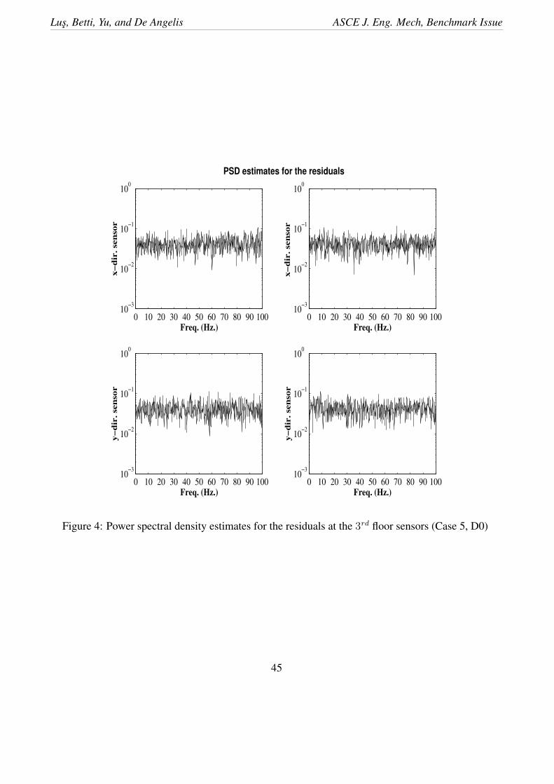
measured and the predicted outputs) are. Fig. 4 shows the power spectral density (PSD) estimates for

the residuals observed at the third floor sensors in Case 5, damage scenario D0. These PSD estimates

show that the residuals indeed resemble white-noise sequences, and therefore it can be concluded that

the identified state-space model is highly capable of reproducing the “true” input-output mapping of

the structure. Once again it should be noted that similar results were obtained in all other cases and

scenarios.

3.2.3 Estimating second-order modal parameters

For classically damped systems, it can be shown that the eigenvalues of a continuous time state-space

model, denoted by σi ± ωi (note that they appear in complex conjugate pairs), are related to the

second-order modal parameters (undamped natural frequencies Ωi and corresponding modal damping

percentages ζi) via

Ωi =√

σ2i + ω2

i ; ζi = − cos(Arctan(ωi

σi

)) (27)

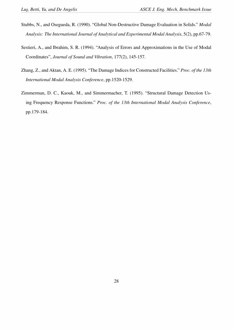
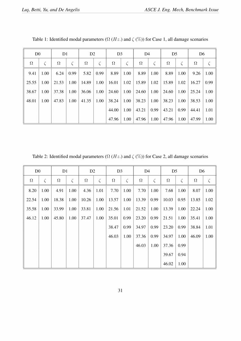
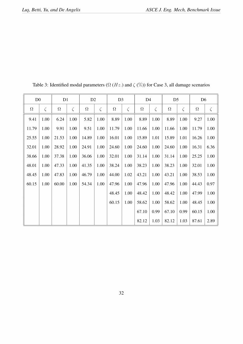
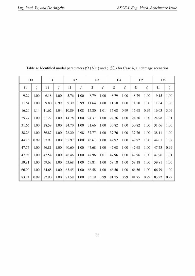
Tables 1 through 5 show such identified parameters for all structural cases and damage scenarios. It is

interesting to note that the number of identifiable modes are not the same for a given case with different

damage scenarios. In fact, when the structure and the loading are symmetric, only translational modes

can be excited and identified, as evidenced in Tables 1, 2, and 3. If, however, a particular damage

scenario induces asymmetry in the structure, then torsional modes can also be identified, as noted in

these tables for the various scenarios of asymmetric damage. Such a problem does not exist if the

14


undamaged structure is asymmetric, as evidenced by the existence of multiple modes in Tables 4, 5

and 6.

Some interesting results were obtained in the analysis of the damage scenario 6 in Cases 5 and

6. For some reason, the first torsional mode of the 120 DOF model, which was previously identified

in scenarios D0-D5 to be around 13-14 Hz., could not be identified in D6. This was an unexpected

phenomenon, in that the higher torsional modes were identified. This can not be attributed to insuffi-

cient instrumentation alone, since this discrepancy appeared in both Case 5 (full instrumentation) and

Case 6 (limited instrumentation). It should be emphasized, however, that this mode does not appear

in the measured structural response. In fact, by obtaining the power spectral density estimates of the

structural accelerations that represent the measured output in the identification process, no peak can

be observed in the frequency range 13-14 Hz., while all the other modes are clearly visible. This,

unfortunately, had repercussions also on the identified physical matrices and on damage detection

efforts.

3.3 Extracting the physical parameters

3.3.1 Choice of cases

In this section we address the identification of the physical parameters, i.e. the mass, damping, and

stiffness matrices, of the underlying second order system, using the identified state-space models. Due

to space limitations, we limit the detailed discussions to three cases, namely Case 3, Case 5, and Case

6. The choice of Case 3 is motivated by the fact that it leads to interesting discussions, since the

number of identifiable modes are different for different damage scenarios, and hence is considered to

be more challenging than Case 4. The choice of Case 5 is motivated by the fact that it is one of the most

difficult cases, since it includes both measurement and modelling errors. Case 6 provides an additional

constraint to Case 5 in that there is a limited number of sensors, i.e. acceleration measurements are

obtained only on the second and the fourth floors.

15


3.3.2 Combining the outputs

In any of the available structural cases, if we assume that the floors are rigid, then the motion of each

floor can be adequately represented by defining translations in x and y directions, and a rotation in

the x-y plane. Each of these variables can be constructed using the available output measurements.

Here we estimate the translation at each floor along the x and y directions by averaging the outputs

of the sensors along the x and y directions, respectively. Analogously, the rotations are estimated by

considering the differences of such outputs, and scaling with the length of the sides of each floor,

since the geometric information regarding the simulated model is available. This modification can be

performed by combining, in a proper manner, the corresponding rows of the output matrices of the

identified state-space models. Following this arrangement amounts to writing the equations of motion

for each floor with respect to its geometric center. Although it is possible to choose other points to

“map” the second-order equations of motion (e.g. the center of mass or the center of stiffness), the

geometric center seems to be the most natural choice since no a priori knowledge of the mass and

stiffness distributions of the models are assumed to be available.

The resulting “new outputs” will be denoted by Xi (translation of the ith floor along the x-direction),

Yi (translation of the ith floor along the y-direction), and Θi (rotation of the ith floor in the x-y plane).

Furthermore, these new outputs will be grouped together such that, for the identified second-order

models, the degrees of freedom will be organized as [X1 . . . X4 Y1 . . . Y4 Θ1 . . . Θ4]. With the help

of these modifications, it will be possible for us to consider partitions of the identified second order

matrices. For example, the partitions of a generic stiffness matrix K will be denoted by KX , KY , and

KΘ, where KX denotes the 4 × 4 partition corresponding to the variables Xi, and KY , and KΘ are

defined analogously. For a perfectly symmetric structure all these partitions are expected to be uncou-

pled, whereas due to asymmetry of the structural system and/or of the damage pattern, “off-diagonal”

elements that couples these partitions may be observed (e.g. coupling between KX and KΘ, or KY

and KΘ).

16


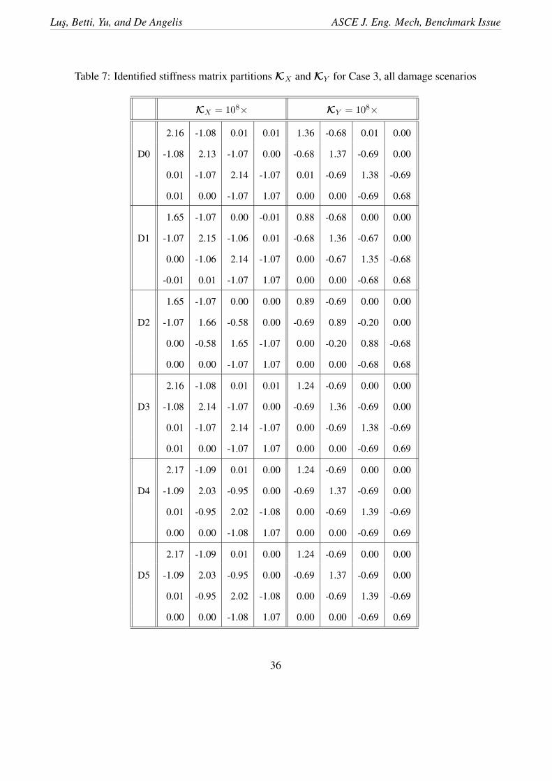
3.3.3 Stiffness matrices for Case 3

For Case 3, in damage scenarios D0, D1, and D2, the structure is completely symmetric, and hence

the number of second-order modes that can be identified is 8. Due to this fact, only an 8 × 8 stiffness

matrix can be constructed (i.e. KΘ can not be estimated), and the identified partitions KX and KY are

shown in Table 7. On the other hand, additional care must be taken when evaluating these partitions

for damage scenarios D3, D4, and D5. In these scenarios, additional modes that were not available

for the reference case can now be identified, since the damage patterns for these scenarios induce

asymmetry in the structure and the ‘torsional’ modes are now excited. In general, there is no problem

in identifying the structural stiffness matrices by including also the contributions of these modes;

however, since the ultimate aim is to identify the changes in the stiffness matrices due to ‘damage’,

even for these scenarios we choose to construct the partitions KX and KY using only the modes that

were also present in the undamaged scenario. Determining which modes appear in both the undamaged

scenario and scenarios D3, D4, and D5 is not a trivial issue since the natural frequencies change due

to damage. Therefore, we must also employ the information in the identified complex mode shapes.

One indicator that determines the correlation of two complex mode shapes ψ i and ψj is the so-called

Modal Amplitude Coherence (MAC) defined as

MACij =|ψH

i ψj|√|ψH

i ψi||ψHj ψj|

(28)

where the superscript ()H denotes complex transpose. When calculating the MAC values, care should

be taken in comparing the complex modes as observed from the output sensors, and only the compo-

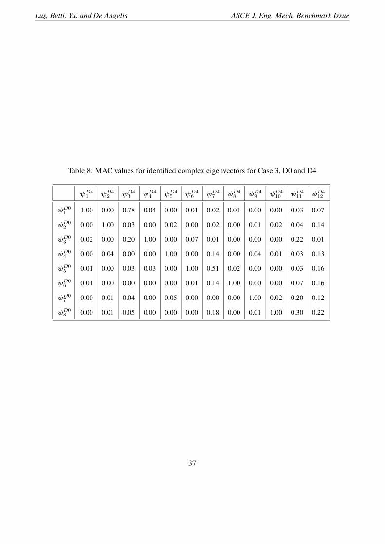
nents corresponding to DOFs Xi and Yi should be included. As an example consider Table 8, which

presents the MAC values that were calculated using the identified complex eigenvectors of the first-

order models for the damage scenarios D0 and D4 (ψD0i refers to an eigenvector for scenario D0,

and ψD4i is defined analogously for D4). Since all modes appear in complex-conjugate pairs, results

for one of each such pair are shown in this table. It can be seen that 4 modes that appear in D4 are

not highly correlated with any of the modes that were identified in D0, and are then associated with

17


the dominantly torsional component of the structural motion. Therefore, for the identification of the

stiffness matrices in scenario D4 (and also for D3 and D5 due to similar reasons), we consider the con-

tribution of only those modes that have a high correlation (i.e. MACij = 1) with the modes identified

in D0. The partitions KX and KY that were identified for D3, D4, and D5 are presented in Table 7.

It should be noted that the effects of noise most readily show up as an artificial coupling phenom-

ena, which can also be observed in the stiffness matrices in Table 7 as non-zero components. However,

even though these components are not zero, their magnitudes are a few orders less than those of the

‘real’ structural stiffnesses, and hence they can be treated essentially as zeros.

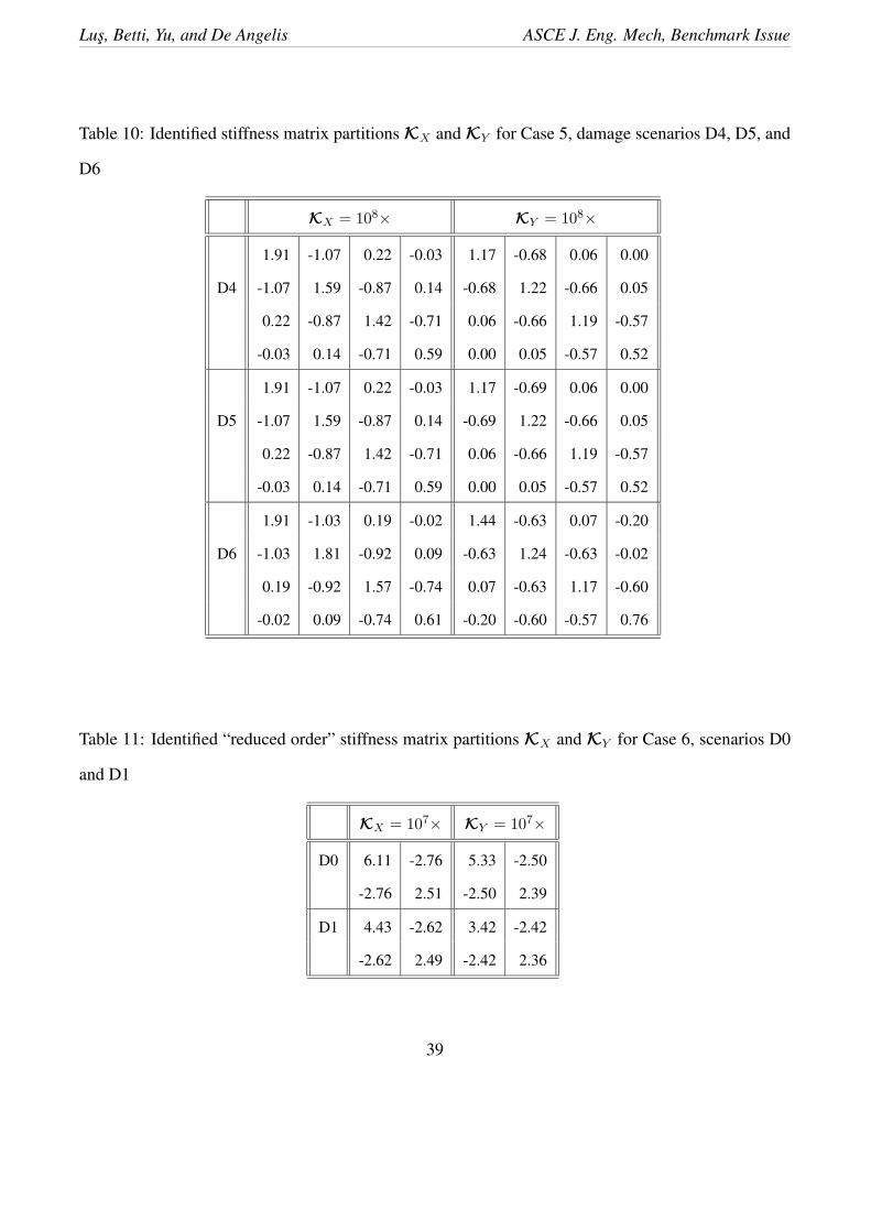
3.3.4 Stiffness Matrices for Case 5

For Case 5, in all scenarios, the asymmetry of the structure allows the identification of 12 second order

modes, and so the second-order models can contain all DOFs Xi, Yi, and Θi. For ease of comparison,

Tables 9 and 10 presents the partitions KX and KY , analogous to the previous case. It is noteworthy

that the asymmetry of the structure shows up as coupling of the partitions in both the mass and the

stiffness matrices, depending on the particular damage scenario.

3.3.5 A Discussion on Case 6

Case 6 poses an interesting problem, for it is now not possible to create “full order” structural ma-

trices. Since the available information only pertains to sensors at the second and the fourth floors,

particular information regarding the first and third floor sensors can not be retrieved via the proposed

methodology. On the other hand, the authors have recently completed a study in which it was shown

that the proposed approach, in the presence of inadequate measurement points, still allows one to con-

struct a stiffness matrix that in fact corresponds to the reduced order form one would obtain through

Guyan reduction. Table 11 presents two of such matrices, namely the reduced order stiffness matri-

ces for damage scenarios D0 and D1. The model in Case 6 is identical to the model in Case 5, but

now the identified reduced order stiffness matrices can not be directly related to structural (e.g. floor)

18


stiffnesses due to the nature of the static condensation operation (the differences between the stiffness

matrix coefficients in Tables 9 and 11 can be attributed to such modifications due to the reduced order

mapping). Nevertheless, changes in these coefficients can still be indicative of structural modifications,

and this issue will be investigated in a later section.

3.4 Detecting ‘Damage’

Once the second-order matrices, representative of the physical parameters of the systems, have been

identified, the structural changes (i.e. ‘damage’) may be located and quantified by comparing the

parameters for the undamaged structure with those of the damaged structures. To this end, we initially

try to locate the damage by investigating the changes in the diagonal elements of the identified stiffness

matrices, and the discussions presented in this section will once again focus on Cases 3, 5, and 6.

Tables 12 and 13 present the relative changes in the identified stiffness matrix partitions KX and

KY for Cases 3 and 5, for all damage scenarios. The values in these tables are calculated via

KDJX (i, i) − K

D0X (i, i)

KD0X (i, i)

(29)

where KDJX (i, i) refers to a diagonal element of the partition KX corresponding to the J th damage

scenario (D1, D2, D3, D4, D5 or D6), and the reference (undamaged) partition is denoted by KD0X (i, i).

Analogous definitions apply to the values related to the partition KY .

The values in these tables indicate that this particular indicator can be used as an initial warning

tool for damage detection, since structural changes show up quite significantly in these values. How-

ever, it should be noted that these parameters may also lead to somewhat misleading conclusions for

small structural changes, since the existence of false predictions (on the order of about 1% to 5%)

can be observed in these tables. These false predictions can be attributed to the distortive effects of

noise (measurement noise and possible modelling errors), and hence real changes on the order of the

aforementioned false predictions can not be detected with high confidence.

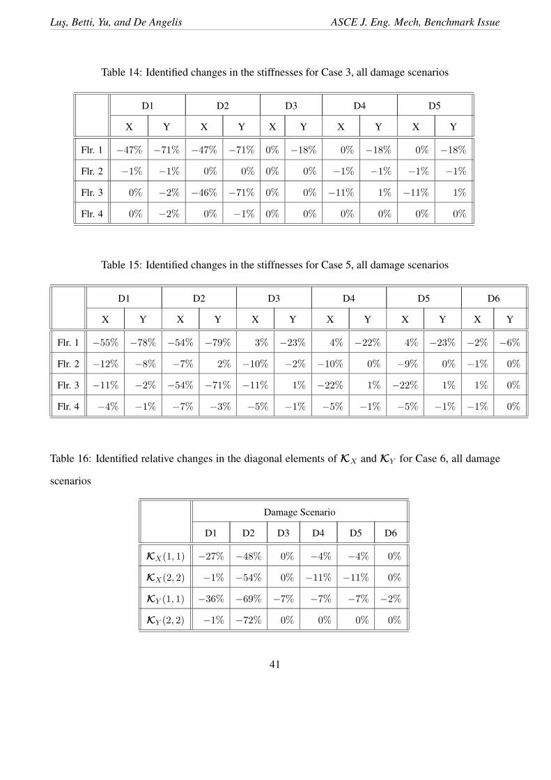
Another point we should note is that the relative changes in these stiffness coefficients can not be

directly related to actual changes at particular locations (e.g. reductions in floor stiffnesses) unless a

19


particular structure (connectivity) for the stiffness is assumed. Instead of making any a priori assump-

tions, it is possible to determine this structure by inspecting the identified stiffness matrices. As an

example, consider the plot of the stiffness matrix coefficients that were identified for the undamaged

structure in Case 3, as presented in Fig. 5. By inspecting this plot, it can be concluded that both KX

(columns 1-4, rows 1-4) and KY (columns 4-8, rows 4-8) are banded matrices, and that the structure

can be analyzed as a shear-type structure along both directions. With this conclusion it is possible

to comment on the reductions in the floor stiffnesses, and Tables 14 and 15 present such estimated

reductions.

On the other hand, the discussions for Case 6 are not so conclusive due to the reduced order map-

ping. Table 16 presents the relative changes in the diagonal elements of the identified reduced order

stiffness matrices, and the values in this table are calculated via eq.(29). In this table, KX(1, 1) and

KY (1, 1) refer to the second floor and KX(2, 2) and KY (2, 2) refer to the fourth floor. As previously

mentioned, the problem is that these changes can not be directly linked to actual structural changes for

quantifying reductions in stiffnesses of particular floors. It is still possible, however, to use this infor-

mation in locating structural changes, such that one can discuss whether a modification has occurred

between the ground level and the second floor, and/or between the second floor and the fourth floor,

along either horizontal direction. Table 17 presents a summary of such an attempt, where the notation

0 − 2 refers to a location between the ground level and the second floor, 2 − 4 refers to a location

between the second floor and the fourth floor, and a check mark denotes that a substantial change in

the stiffness, which can be attributed to a damage, has occurred. It should be noted that, in constructing

this table, variations up to 5% have been considered as false alarms, since such a perturbation is within

the realm of the effects of noise for the 120 DOF model. It can be seen that the proposed method-

ology is quite successful in locating the damage with regards to available locations, for all scenarios

considered.

It should be noted that, for Cases 5 and 6 and damage scenario D6, the comparisons presented

in the aforementioned tables were articulated using only the translational modes in constructing the

20


stiffness matrices for comparison of D0 and D6. This approach was motivated by the fact that the first

torsional mode could not be identified in D6, and hence, the comparison was carried out using only

the contribution of the translational modes to evaluate the structural changes between D0 and D6, for

Cases 5 and 6.

4 Discussions

In the light of the preceding discussions, the following points should be further commented on:

• The proposed methodology has proven to be quite accurate in determining state-space mod-

els from given input-output data, for all structural models and damage scenarios considered in

the first part of the benchmark investigation. This remark is supported by the performance of

the identified first-order models in predicting (reproducing) the structural response, which were

shown to be quite effective as discussed in section 3.2.2.

• One of the main advantages of using a state space model is that no data manipulation (integration

or differentiation) is required for the identification. In this analysis, only the time histories of

the structural accelerations have been directly used, without any pre-filtering, and structural

velocities and/or displacements were not used (or required) at any stage of the identification.

• It was mentioned that for classically damped systems, the second-order modal parameters can

be directly retrieved from the continuous-time eigenvalues of the identified state-space model.

In general, the second-order system might have coupled modes, and in such cases one must

first identify the mass and stiffness parameters to obtain undamped modal parameters. The

methodology presented in section 2.3 allows such a construction, and does not require any a

priori assumptions on the nature and type of structural damping.

• The main differences obtained in the identification results were observed in the structural models

of the 12 DOF and 120 DOF systems. In all cases related to the 12 DOF system, the identified

21


stiffness matrices displayed a banded structure, and a shear-type modelling was well justified.

On the other hand, in the cases related to the 120 DOF model, the banded structure of the

identified stiffness matrices were disrupted by other elements of comparable magnitude (see, for

example, Table 9, KX(1, 3) and KX(3, 1)). However, the presence of such elements can not be

attributed only to measurement noise. Even if one uses noise-free data, such off-band elements

still appear in the analysis of the 120 DOF cases (although they are identically equal to zero for

12 DOF cases). These discrepancies can perhaps be attributed to some modelling error inherent

to the 120 DOF cases.

• In terms of the identified damage, there does not seem to be a substantial difference between

damage scenarios 4 and 5. This may be justified if the difference in the damage patterns simply

does not show up in the data matrices that are used in the data generation program (which is

suspected to be the case for the 12 DOF cases), or if the difference is so small that it was not

possible to differentiate its effects due to very low signal to noise ratio. For example, in Case

5, even though there seems to be a small difference in the identified frequencies for damage

scenarios 4 and 5 (D4 and D5), these differences induce only a 1% maximum difference in the

reduction of the floor stiffnesses. However, such a small margin must be considered to be within

the noise tolerance, and hence can not be directly attributed to a real damage.

• Damage scenario D6, which was to be included in the analysis of Case 5 and Case 6, proved to be

more problematic than the other damage scenarios. The main problem, as previously mentioned,

is that the first torsional mode does not appear in the identification results for D6, even though

all the other modes can be successfully identified. The first torsional mode can be identified

when no measurement noise is considered; however, with the addition of noise in the data, its

contribution can not be observed. This phenomenon is all the more clear if one investigates the

power spectral densities of the acceleration time histories, for there does not seem to appear

any peak in the frequency range 13-14 Hz. This proves to be a difficulty because of the nature

of the damage itself: since the changes induced in the model are very small, missing out one

22


of the fundamental modes apparently has a strong effect on the identifiability of such changes.

As previously mentioned, it was possible to account for only the translational modes, and the

changes in the diagonal elements of the identified stiffness matrices were presented in Tables 13

and 16.

• For Case 6, the number of sensors was a limiting factor in determining the structural damage.

Since the methodology relies only on input-output data and no a priori model is employed, it

was only possible to obtain reduced order mass, damping, and stiffness matrices. This reduced

order mapping refrained us from being able to directly comment on the reductions of particular

floor or element stiffnesses. However, it was still possible to locate damaged areas with respect

to the locations of the available sensors. No damage quantification was possible due to the

nature of the reduced order mapping, and to the fact that no a priori information on the stiffness

matrix was available. Moreover, for damage scenario D6, the identified changes were within the

error margin (noise tolerance), and hence, it was not possible to finalize a decision regarding the

location of the damaged area (as evidenced in Table 17).

• In general, it should be mentioned that the number of available sensors and actuators greatly

effects the mapping of the damage on a structure. When one indeed works with a finite DOF

system, and if the number of sensors and actuators is sufficient for a full order mapping to

a finite element model, the methodology may be expected to be able to map the damage to

structural elements. When, however, the number of instrumentation is not adequate for a full

order mapping, the best one can hope for is a reduced order model that somehow contains,

in its stiffness coefficients, the information regarding possible damage. In fact, the authors

have recently shown that in such cases it is possible obtain a reduced order stiffness matrix that

corresponds to statically condensing the un-instrumented DOFs of the full order model (Lus

et al., 2002). In the case of insufficient instrumentation, however, it may be anticipated that the

methodology will be able to predict the existence and map the location of damage with reference

to the existing sensor-actuator locations, but that it will not be able to exactly quantify the amount

23


of damage in a structural element unless it is supplemented by other information, such as an a

priori knowledge of the location of damage, an initial analytical finite element model, etc..

• Even with such considerations, the proposed methodology has proven to be an efficient tool in

detecting structural damage, at least in this part of the benchmark analysis. The errors in such

damage predictions are determined mainly by the limitations of the assumed behavior of the

identified second-order model, and its ability to represent the ‘true’ system. It has been observed

that the damage predictions for the 12 DOF cases were subject to less variations, or equivalently

they were less sensitive to perturbations, than their 120 DOF counterparts.

• It should be strongly emphasized that no a priori knowledge regarding any property (except for

the geometric dimensions) of the models under investigation were assumed to be known. The

algorithm is almost a black-box type approach that creates a second-order system that ‘best’ fits

the given input-output data, with the help of an intermediary state-space model. The inherent

flexibility of state-space models in creating good fits of input-output mapping, combined with the

formulations discussed in section 2.3, increases the robustness of the proposed hybrid approach.

5 Conclusions

In this paper, a two-stage system identification methodology has been presented and applied to dam-

age detection for the case of the benchmark problem proposed by the ASCE Task Group on Health

Monitoring. First, a first-order state-space model of the structural system is identified using only the

available input-output measurement data and then, such a model is converted to a second-order mass,

damping and stiffness model. It does not require any numerical manipulation (integration, differen-

tiation, filtering) of the recorder data and does not impose any limitation on the nature and type of

structural damping and on the coupling of the vibrational modes. The only requirements are the pres-

ence of one sensor-actuator co-located pair and the knowledge of the sensors and actuators locations.

The location and quantification of the structural damage is determined by comparing the identified

24


stiffness matrices for the undamaged and damaged case. The numerical results for all the cases con-

tained in the benchmark problem provide a good estimation of the location and amount of structural

damage, even in the presence of substantial measurement noise and possible modelling errors.

Acknowledgements

This research has been sponsored through a research grant by the National Science Foundation (CMS-

9457305) whose supprt has been greatly appreciated.

25


APPENDIX I.

References

Agbabian, M. S., Masri, S. F., Miller, R. K., and Caughey, T. K. (1991). “System Identification

Approach to Detection of Structural Changes”, ASCE Journal of Engineering Mechanics, 117(2),

pp.370-390.

Balmes, E. (1997). “New Results on the Identification of Normal Modes from Experimental Complex

Modes”, Mechanical Systems and Signal Processing, 11(2), 229-243.

De Angelis, M., Lus, H., Betti, R., and Longman, R.W. (2002). “Extracting Physical Parameters of

Mechanical Models from Identified State Space Representations”, ASME Journal of Engineering

Mechanics, 69(9), pp.617-625.

Doebling, S. W., Farrar, C. H., Prime, M. B., and Shevitz, D. W. (1996). “Damage Identification

and Health Monitoring of Structural and Mechanical Systems From Changes In Their Vibration

Characteristics: A Literature Review”, Los Alamos National Laboratory Technical Report, LA-

13070-MS.

Friswell, M. I., Penny, J. E. T., and Wilson (1994). “Using Vibration Data and Statistical Measures

to Locate Damage in Structures.” Modal Analysis: The International Journal of Analytical and

Experimental Modal Analysis, 9(4), pp.239-254.

Hassiotis S., and Jeong, G. D., (1995). “Identification of Stiffness Reductions Using Natural Frequen-

cies.” ASCE Journal of Engineering Mechanics, 121(10), pp.1106-1113.

Juang, J.-N. and Pappa, R.S. (1985). “An Eigensystem Realization Algorithm for Model Parameter

Identification and Model Reduction.” Journal of Guidance, Control, and Dynamics, 8(5), 620-627.

Juang, J.-N., Phan, M., Horta, L.G., and Longman, R.W. (1993). “Identification of Observer/Kalman

26


Filter Markov Parameters: Theory and Experiments.” Journal of Guidance, Control, and Dynamics,

16(2), 320-329.

Juang, J.-N., and Longman, R.W., (1999). “Optimized System Identification.” NASA Technical Mem-

orandum, NASA/TM-1999-209711.

Lus, H., Betti, R., and Longman, R.W. (1999). “Identification of Linear Structural Systems Using

Earthquake-Induced Vibration Data.” Earthquake Engineering and Structural Dynamics, 28, 1449-

1467.

Lus, H. (2001). Control Theory Based System Identification. Ph.D. Thesis, Columbia University, New

York.

Lus, H., Betti, R., and Longman, R.W. (2002). “Obtaining Refined First Order Predictive Models of

Linear Structural Systems.” Earthquake Engineering and Structural Dynamics, 31, pp.1413-1440.

Lus, H., De Angelis, M. and Betti, R. (2002). “A New Approach for Reduced Order Modeling of

Mechanical Systems Using Vibration Measurements”, submitted to ASME Journal of Applied Me-

chanics.

Peterson, L. D., Alvin, K. F., Doebling, S. W., and Park, K. C. (1993). “Damage De-

tection Using Experimentally Measured Mass and Stiffness Matrices.” Proc. of the 34th

AIAA/ASME/ASCE/AHS/ASC Structures, Structural Dynamics, and Materials Conference, AIAA-

93-1482-CP, pp.1518-1528.

Ricles, J. M. (1991). “Nondestructive Structural Damage Detection in Flexible Space Structures Using

Vibration Characterization.” NASA Technical Report, CR-185670.

Smyth, A. W., Masri, S. F., Caughey, T. K., and Hunter, N. F. (2000). “Surveillance of Intricate Me-

chanical Systems on the Basis of Vibration Signature Analysis”, ASME Journal of Applied Mechan-

ics, 67(3), pp.540-551.

27


Stubbs, N., and Osegueda, R. (1990). “Global Non-Destructive Damage Evaluation in Solids.” Modal

Analysis: The International Journal of Analytical and Experimental Modal Analysis, 5(2), pp.67-79.

Sestieri, A., and Ibrahim, S. R. (1994). “Analysis of Errors and Approximations in the Use of Modal

Coordinates”, Journal of Sound and Vibration, 177(2), 145-157.

Zhang, Z., and Aktan, A. E. (1995). “The Damage Indices for Constructed Facilities.” Proc. of the 13th

International Modal Analysis Conference, pp.1520-1529.

Zimmerman, D. C., Kaouk, M., and Simmermacher, T. (1995). “Structural Damage Detection Us-

ing Frequency Response Functions.” Proc. of the 13th International Modal Analysis Conference,

pp.179-184.

28


List of Tables

1 Identified modal parameters (Ω (Hz.) and ζ (%)) for Case 1, all damage scenarios . . . 31






7 Identified stiffness matrix partitions KX and KY for Case 3, all damage scenarios . . . 36

8 MAC values for identified complex eigenvectors for Case 3, D0 and D4 . . . . . . . . 37

9 Identified stiffness matrix partitions KX and KY for Case 5, damage scenarios D0,

D1, D2, and D3 . . . . . . . . . . . . . . . . . . . . . . . . . . . . . . . . . . . . . . 38

10 Identified stiffness matrix partitions KX and KY for Case 5, damage scenarios D4,

D5, and D6 . . . . . . . . . . . . . . . . . . . . . . . . . . . . . . . . . . . . . . . . 39

11 Identified “reduced order” stiffness matrix partitions KX and KY for Case 6, scenarios

D0 and D1 . . . . . . . . . . . . . . . . . . . . . . . . . . . . . . . . . . . . . . . . . 39

12 Identified relative changes in the diagonal elements of KX and KY for Case 3, all

damage scenarios . . . . . . . . . . . . . . . . . . . . . . . . . . . . . . . . . . . . . 40



14 Identified changes in the stiffnesses for Case 3, all damage scenarios . . . . . . . . . . 41

15 Identified changes in the stiffnesses for Case 5, all damage scenarios . . . . . . . . . . 41



17 Identified damage locations and directions for Case 6, all damage scenarios . . . . . . 42

29


List of Figures

1 Singular values of the Hankel matrix for Case 1, D0 . . . . . . . . . . . . . . . . . . . 43

2 Singular values of the Hankel matrix for Case 1, D3 . . . . . . . . . . . . . . . . . . . 43

3 Estimates for magnitudes of the transfer functions for 3rd floor sensors (Case 5, D0) . 44

4 Power spectral density estimates for the residuals at the 3rd floor sensors (Case 5, D0) 45

5 Elements of the 8 × 8 stiffness matrix for the undamaged model in Case 3 . . . . . . . 46

30


Table 1: Identified modal parameters (Ω (Hz.) and ζ (%)) for Case 1, all damage scenarios

D0 D1 D2 D3 D4 D5 D6

Ω ζ Ω ζ Ω ζ Ω ζ Ω ζ Ω ζ Ω ζ

9.41 1.00 6.24 0.99 5.82 0.99 8.89 1.00 8.89 1.00 8.89 1.00 9.26 1.00

25.55 1.00 21.53 1.00 14.89 1.00 16.01 1.02 15.89 1.02 15.89 1.02 16.27 0.99

38.67 1.00 37.38 1.00 36.06 1.00 24.60 1.00 24.60 1.00 24.60 1.00 25.24 1.00

48.01 1.00 47.83 1.00 41.35 1.00 38.24 1.00 38.23 1.00 38.23 1.00 38.53 1.00

44.00 1.00 43.21 0.99 43.21 0.99 44.41 1.01

47.96 1.00 47.96 1.00 47.96 1.00 47.99 1.00


D0 D1 D2 D3 D4 D5 D6


8.20 1.00 4.91 1.00 4.36 1.01 7.70 1.00 7.70 1.00 7.68 1.00 8.07 1.00

22.54 1.00 18.38 1.00 10.26 1.00 13.57 1.00 13.39 0.99 10.03 0.95 13.85 1.02

35.58 1.00 33.99 1.00 33.81 1.00 21.56 1.01 21.52 1.00 13.39 1.00 22.24 1.00

46.12 1.00 45.80 1.00 37.47 1.00 35.01 0.99 23.20 0.99 21.51 1.00 35.41 1.00

38.47 0.99 34.97 0.99 23.20 0.99 38.84 1.01

46.03 1.00 37.36 0.99 34.97 1.00 46.09 1.00

46.03 1.00 37.36 0.99

39.67 0.94

46.02 1.00

31



D0 D1 D2 D3 D4 D5 D6


9.41 1.00 6.24 1.00 5.82 1.00 8.89 1.00 8.89 1.00 8.89 1.00 9.27 1.00

11.79 1.00 9.91 1.00 9.51 1.00 11.79 1.00 11.66 1.00 11.66 1.00 11.79 1.00

25.55 1.00 21.53 1.00 14.89 1.00 16.01 1.00 15.89 1.01 15.89 1.01 16.26 1.00

32.01 1.00 28.92 1.00 24.91 1.00 24.60 1.00 24.60 1.00 24.60 1.00 16.31 6.36

38.66 1.00 37.38 1.00 36.06 1.00 32.01 1.00 31.14 1.00 31.14 1.00 25.25 1.00

48.01 1.00 47.33 1.00 41.35 1.00 38.24 1.00 38.23 1.00 38.23 1.00 32.01 1.00

48.45 1.00 47.83 1.00 46.79 1.00 44.00 1.02 43.21 1.00 43.21 1.00 38.53 1.00

60.15 1.00 60.00 1.00 54.34 1.00 47.96 1.00 47.96 1.00 47.96 1.00 44.43 0.97

48.45 1.00 48.42 1.00 48.42 1.00 47.99 1.00

60.15 1.00 58.62 1.00 58.62 1.00 48.45 1.00

67.10 0.99 67.10 0.99 60.15 1.00

82.12 1.03 82.12 1.03 87.61 2.89

32



D0 D1 D2 D3 D4 D5 D6


9.29 1.00 6.18 1.00 5.76 1.00 8.79 1.00 8.79 1.00 8.79 1.00 9.15 1.00

11.64 1.00 9.80 0.99 9.39 0.99 11.64 1.00 11.50 1.00 11.50 1.00 11.64 1.00

16.20 1.14 11.62 1.04 10.89 1.08 15.80 1.01 15.68 0.99 15.68 0.99 16.03 3.09

25.27 1.00 21.27 1.00 14.78 1.00 24.37 1.00 24.36 1.00 24.36 1.00 24.98 1.01

31.66 1.00 28.59 1.00 24.70 1.00 31.66 1.00 30.82 1.00 30.82 1.00 31.66 1.00

38.26 1.00 36.87 1.00 28.20 0.98 37.77 1.00 37.76 1.00 37.76 1.00 38.11 1.00

44.25 0.99 37.93 1.00 35.97 1.00 43.61 1.00 42.92 1.00 42.92 1.00 44.01 1.02

47.75 1.00 46.81 1.00 40.60 1.00 47.68 1.00 47.68 1.00 47.68 1.00 47.73 0.99

47.96 1.00 47.54 1.00 46.46 1.00 47.96 1.01 47.96 1.00 47.96 1.00 47.96 1.01

59.81 1.00 59.63 1.00 53.68 1.00 59.81 1.00 58.18 1.00 58.18 1.00 59.81 1.00

66.90 1.00 64.68 1.00 63.45 1.00 66.58 1.00 66.56 1.00 66.56 1.00 66.79 1.00

83.24 0.99 82.90 1.00 71.58 1.00 83.19 0.99 81.75 0.99 81.75 0.99 83.22 0.99

33



D0 D1 D2 D3 D4 D5 D6


8.09 0.99 4.86 1.00 4.30 0.99 7.61 1.00 7.61 1.00 7.58 1.00 7.96 1.00

8.40 1.01 6.53 1.00 5.69 1.00 8.40 1.00 8.13 1.00 8.13 1.00 8.40 1.00

13.79 1.03 8.74 0.96 7.66 1.00 13.38 0.97 13.21 1.00 13.21 1.00 17.80 1.73

22.27 1.00 18.12 1.00 10.21 1.00 21.34 1.00 21.30 1.00 21.29 1.00 21.99 1.00

23.92 1.00 20.77 1.00 15.12 1.00 23.92 1.00 22.95 1.00 22.95 1.00 23.92 1.00

35.21 1.00 32.13 1.00 18.21 0.99 34.55 1.00 34.49 1.00 34.49 1.00 35.01 1.00

38.58 0.99 33.62 1.00 33.53 1.00 38.11 1.01 37.20 1.00 37.20 1.00 38.40 1.05

39.44 1.00 37.68 1.00 37.00 1.00 39.41 1.00 39.17 1.00 39.17 1.00 39.42 1.00

45.95 1.00 45.61 1.00 37.29 1.00 45.84 1.00 45.84 1.00 45.83 1.00 45.91 1.00

55.02 1.00 54.52 1.00 47.63 1.00 55.02 1.00 53.16 1.00 53.16 1.00 55.02 1.00

60.22 1.01 57.51 1.01 57.49 1.01 59.83 1.01 59.82 1.01 59.82 1.01 60.09 1.01

79.22 1.00 78.51 1.01 65.82 1.00 79.11 1.01 77.49 0.99 77.49 0.99 79.18 1.00

34



D0 D1 D2 D3 D4 D5 D6


8.09 0.99 4.86 1.01 4.30 0.99 7.61 1.00 7.61 1.00 7.58 1.00 7.96 1.00

8.40 1.01 6.53 1.01 5.69 1.00 8.40 1.01 8.13 1.00 8.13 0.99 8.40 1.01

13.78 1.06 8.74 1.04 7.66 0.94 13.39 0.97 13.21 1.03 13.21 0.99

22.27 1.01 18.12 0.99 10.21 1.00 21.34 1.00 21.30 1.00 21.29 1.00 21.99 1.00

23.92 1.00 20.77 1.00 15.11 1.00 23.92 1.00 22.96 1.00 22.96 1.00 23.92 1.00

35.22 1.00 32.13 1.00 18.22 0.95 34.54 1.00 34.49 1.00 34.49 1.00 35.01 1.01

38.58 1.00 33.62 1.00 33.53 1.00 38.11 1.02 37.20 1.00 37.20 1.00 38.35 1.15

39.44 1.00 37.68 1.00 37.00 1.00 39.41 1.00 39.17 1.00 39.17 1.00 39.42 1.01

45.95 1.00 45.60 1.01 37.30 1.01 45.84 1.00 45.84 1.01 45.83 1.01 45.91 1.00

55.02 1.00 54.51 1.00 47.63 1.00 55.02 1.00 53.17 1.00 53.17 1.00 55.02 1.00

60.22 1.00 57.52 1.02 57.49 1.01 59.84 1.00 59.82 1.01 59.82 1.00 60.09 1.01

79.21 1.02 78.51 1.01 65.82 0.99 79.11 1.02 77.49 0.99 77.49 0.99 79.18 1.02

35


Table 7: Identified stiffness matrix partitions KX and KY for Case 3, all damage scenarios

KX = 108× KY = 108×

2.16 -1.08 0.01 0.01 1.36 -0.68 0.01 0.00

D0 -1.08 2.13 -1.07 0.00 -0.68 1.37 -0.69 0.00

0.01 -1.07 2.14 -1.07 0.01 -0.69 1.38 -0.69

0.01 0.00 -1.07 1.07 0.00 0.00 -0.69 0.68

1.65 -1.07 0.00 -0.01 0.88 -0.68 0.00 0.00

D1 -1.07 2.15 -1.06 0.01 -0.68 1.36 -0.67 0.00

0.00 -1.06 2.14 -1.07 0.00 -0.67 1.35 -0.68

-0.01 0.01 -1.07 1.07 0.00 0.00 -0.68 0.68

1.65 -1.07 0.00 0.00 0.89 -0.69 0.00 0.00

D2 -1.07 1.66 -0.58 0.00 -0.69 0.89 -0.20 0.00

0.00 -0.58 1.65 -1.07 0.00 -0.20 0.88 -0.68

0.00 0.00 -1.07 1.07 0.00 0.00 -0.68 0.68

2.16 -1.08 0.01 0.01 1.24 -0.69 0.00 0.00

D3 -1.08 2.14 -1.07 0.00 -0.69 1.36 -0.69 0.00

0.01 -1.07 2.14 -1.07 0.00 -0.69 1.38 -0.69

0.01 0.00 -1.07 1.07 0.00 0.00 -0.69 0.69

2.17 -1.09 0.01 0.00 1.24 -0.69 0.00 0.00

D4 -1.09 2.03 -0.95 0.00 -0.69 1.37 -0.69 0.00

0.01 -0.95 2.02 -1.08 0.00 -0.69 1.39 -0.69

0.00 0.00 -1.08 1.07 0.00 0.00 -0.69 0.69

2.17 -1.09 0.01 0.00 1.24 -0.69 0.00 0.00

D5 -1.09 2.03 -0.95 0.00 -0.69 1.37 -0.69 0.00

0.01 -0.95 2.02 -1.08 0.00 -0.69 1.39 -0.69

0.00 0.00 -1.08 1.07 0.00 0.00 -0.69 0.69

36


Table 8: MAC values for identified complex eigenvectors for Case 3, D0 and D4

ψD41 ψD4

2 ψD43 ψD4

4 ψD45 ψD4

6 ψD47 ψD4

8 ψD49 ψD4

10 ψD411 ψD4

12

ψD01 1.00 0.00 0.78 0.04 0.00 0.01 0.02 0.01 0.00 0.00 0.03 0.07

ψD02 0.00 1.00 0.03 0.00 0.02 0.00 0.02 0.00 0.01 0.02 0.04 0.14

ψD03 0.02 0.00 0.20 1.00 0.00 0.07 0.01 0.00 0.00 0.00 0.22 0.01

ψD04 0.00 0.04 0.00 0.00 1.00 0.00 0.14 0.00 0.04 0.01 0.03 0.13

ψD05 0.01 0.00 0.03 0.03 0.00 1.00 0.51 0.02 0.00 0.00 0.03 0.16

ψD06 0.01 0.00 0.00 0.00 0.00 0.01 0.14 1.00 0.00 0.00 0.07 0.16

ψD07 0.00 0.01 0.04 0.00 0.05 0.00 0.00 0.00 1.00 0.02 0.20 0.12

ψD08 0.00 0.01 0.05 0.00 0.00 0.00 0.18 0.00 0.01 1.00 0.30 0.22

37


Table 9: Identified stiffness matrix partitions KX and KY for Case 5, damage scenarios D0, D1, D2,

and D3

KX = 108× KY = 108×

1.99 -1.19 0.33 -0.08 1.31 -0.69 0.05 0.01

D0 -1.19 1.85 -1.11 0.20 -0.69 1.22 -0.65 0.05

0.33 -1.11 1.62 -0.75 0.05 -0.65 1.19 -0.58

-0.08 0.20 -0.75 0.60 0.01 0.05 -0.58 0.52

1.40 -1.04 0.21 -0.03 0.77 -0.63 0.03 0.01

D1 -1.04 1.68 -0.99 0.15 -0.63 1.17 -0.64 0.05

0.21 -0.99 1.54 -0.71 0.03 -0.64 1.18 -0.57

-0.03 0.15 -0.71 0.58 0.01 0.05 -0.57 0.52

1.47 -1.10 0.21 -0.04 0.83 -0.70 0.07 -0.02

D2 -1.10 1.27 -0.51 0.13 -0.70 0.78 -0.19 0.05

0.21 -0.51 1.04 -0.69 0.07 -0.19 0.70 -0.56

-0.04 0.13 -0.69 0.58 -0.02 0.05 -0.56 0.53

1.90 -1.07 0.21 -0.02 1.16 -0.68 0.07 0.00

D3 -1.07 1.71 -0.99 0.14 -0.68 1.22 -0.66 0.05

0.21 -0.99 1.53 -0.71 0.07 -0.66 1.19 -0.57

-0.02 0.14 -0.71 0.58 0.00 0.05 -0.57 0.52

38


Table 10: Identified stiffness matrix partitions KX and KY for Case 5, damage scenarios D4, D5, and

D6

KX = 108× KY = 108×

1.91 -1.07 0.22 -0.03 1.17 -0.68 0.06 0.00

D4 -1.07 1.59 -0.87 0.14 -0.68 1.22 -0.66 0.05

0.22 -0.87 1.42 -0.71 0.06 -0.66 1.19 -0.57

-0.03 0.14 -0.71 0.59 0.00 0.05 -0.57 0.52

1.91 -1.07 0.22 -0.03 1.17 -0.69 0.06 0.00

D5 -1.07 1.59 -0.87 0.14 -0.69 1.22 -0.66 0.05

0.22 -0.87 1.42 -0.71 0.06 -0.66 1.19 -0.57

-0.03 0.14 -0.71 0.59 0.00 0.05 -0.57 0.52

1.91 -1.03 0.19 -0.02 1.44 -0.63 0.07 -0.20

D6 -1.03 1.81 -0.92 0.09 -0.63 1.24 -0.63 -0.02

0.19 -0.92 1.57 -0.74 0.07 -0.63 1.17 -0.60

-0.02 0.09 -0.74 0.61 -0.20 -0.60 -0.57 0.76

Table 11: Identified “reduced order” stiffness matrix partitions KX and KY for Case 6, scenarios D0

and D1

KX = 107× KY = 107×

D0 6.11 -2.76 5.33 -2.50

-2.76 2.51 -2.50 2.39

D1 4.43 -2.62 3.42 -2.42

-2.62 2.49 -2.42 2.36

39


Table 12: Identified relative changes in the diagonal elements of KX and KY for Case 3, all damage

scenarios

Damage Scenario

D1 D2 D3 D4 D5

KX(1, 1) −24% −24% 0% 1% 1%

KX(2, 2) 1% −22% 0% −5% −5%

KX(3, 3) 0% −23% 0% −6% −6%

KX(4, 4) −1% −1% 0% 0% 0%

KY (1, 1) −36% −35% −9% −8% −8%

KY (2, 2) −1% −35% 0% 0% 0%

KY (3, 3) −2% −36% 1% 1% 1%

KY (4, 4) −3% 1% 0% 1% 1%


scenarios

Damage Scenario

D1 D2 D3 D4 D5 D6

KX(1, 1) −30% −26% −5% −4% −4% −1%

KX(2, 2) −9% −32% −7% −14% −14% 0%

KX(3, 3) −5% −36% −6% −13% −13% −1%

KX(4, 4) −2% −2% −3% −2% −2% −1%

KY (1, 1) −41% −37% −12% −11% −11% −3%

KY (2, 2) −4% −36% 0% 0% 0% 0%

KY (3, 3) −1% −42% −1% 0% 0% 0%

KY (4, 4) −1% 1% −1% −1% −1% 0%

40


Table 14: Identified changes in the stiffnesses for Case 3, all damage scenarios

D1 D2 D3 D4 D5

X Y X Y X Y X Y X Y

Flr. 1 −47% −71% −47% −71% 0% −18% 0% −18% 0% −18%

Flr. 2 −1% −1% 0% 0% 0% 0% −1% −1% −1% −1%

Flr. 3 0% −2% −46% −71% 0% 0% −11% 1% −11% 1%

Flr. 4 0% −2% 0% −1% 0% 0% 0% 0% 0% 0%

Table 15: Identified changes in the stiffnesses for Case 5, all damage scenarios

D1 D2 D3 D4 D5 D6

X Y X Y X Y X Y X Y X Y

Flr. 1 −55% −78% −54% −79% 3% −23% 4% −22% 4% −23% −2% −6%

Flr. 2 −12% −8% −7% 2% −10% −2% −10% 0% −9% 0% −1% 0%

Flr. 3 −11% −2% −54% −71% −11% 1% −22% 1% −22% 1% 1% 0%

Flr. 4 −4% −1% −7% −3% −5% −1% −5% −1% −5% −1% −1% 0%


scenarios

Damage Scenario

D1 D2 D3 D4 D5 D6

KX(1, 1) −27% −48% 0% −4% −4% 0%

KX(2, 2) −1% −54% 0% −11% −11% 0%

KY (1, 1) −36% −69% −7% −7% −7% −2%

KY (2, 2) −1% −72% 0% 0% 0% 0%

41


Table 17: Identified damage locations and directions for Case 6, all damage scenarios

Damage Direction Location

Scenario 0-2 2-4

D1 x X

y X

D2 x X X

y X X

D3 x

y X

D4 x X

y X

D5 x X

y X

D6 x

y

42


0 2 4 6 8 10 12 14 16 18 2010−4

10−3

10−2

10−1

100

101

102

Number

SV

Mag

nit

ud

e

Hankel Matrix Singular Values

Figure 1: Singular values of the Hankel matrix for Case 1, D0

0 2 4 6 8 10 12 14 16 18 2010−1

100

101

102

Number

SV

Mag

nit

ud

e

Hankel Matrix Singular Values

Figure 2: Singular values of the Hankel matrix for Case 1, D3

43


0 10 20 30 40 50 60 70 80 90 100

10−6

10−4

10−2

Freq. (Hz.)

x−d

ir. s

enso

r

"measured" reconstructed

0 10 20 30 40 50 60 70 80 90 10010−6

10−5

10−4

10−3

10−2

Freq.(Hz.)

x−d

ir. s

enso

r

0 10 20 30 40 50 60 70 80 90 10010−8

10−6

10−4

10−2

Freq. (Hz.)

y−d

ir. s

enso

r

0 10 20 30 40 50 60 70 80 90 100

10−6

10−4

10−2

Freq. (Hz.)

y−d

ir. s

enso

r

Magnitudes of the "measured" and "reconstructed" transfer functions

Figure 3: Estimates for magnitudes of the transfer functions for 3rd floor sensors (Case 5, D0)

44


0 10 20 30 40 50 60 70 80 90 10010−3

10−2

10−1

100

Freq. (Hz.)

x−d

ir. s

enso

r

0 10 20 30 40 50 60 70 80 90 10010−3

10−2

10−1

100

Freq. (Hz.)

x−d

ir. s

enso

r

0 10 20 30 40 50 60 70 80 90 10010−3

10−2

10−1

100

Freq. (Hz.)

y−d

ir. s

enso

r

0 10 20 30 40 50 60 70 80 90 10010−3

10−2

10−1

100

Freq. (Hz.)

y−d

ir. s

enso

r

PSD estimates for the residuals

Figure 4: Power spectral density estimates for the residuals at the 3rd floor sensors (Case 5, D0)

45


12345678

1 2 3 4 5 6 7 8−2

−1.5

−1

−0.5

0

0.5

1

1.5

2

x 108

Elements of the identified stiffness matrix for Case 3, D0

K(i

,j)

Figure 5: Elements of the 8 × 8 stiffness matrix for the undamaged model in Case 3

46