Initial Design and Simulation of the Attitude Determination and Control System for LightSail-1

A Senior Project

presented to

the Faculty of the Aerospace Engineering Department

California Polytechnic State University, San Luis Obispo

In Partial Fulfillment

of the Requirements for the Degree

Bachelor of Science

by

Matthew Thomas Nehrenz

June, 2010

© 2010 Matthew Thomas Nehrenz

Initial Design and Simulation of the Attitude Determination and Control System for LightSail-1

This paper discusses the design and simulation of LightSail-1’s attitude determination and control system. LightSail-1 will launch in 2011 and deploy a 32 m2 mylar sail from a 3U CubeSat with the intent of measuring thrust from solar pressure and raising the orbit. The spacecraft will be actively controlled with magnetorquers and a momentum wheel. The various control modes throughout the short mission lifetime include detumble, sun-pointing, and orbit raising. Each one of these modes is simulated in MatLab, and the assumptions and limitations of the MatLab model are discussed. The simulations show that the spacecraft will detumble in 90 minutes after ejection from the P-POD and demonstrate successful sun-pointing within two orbit periods. Orbit raising will require two rapid 90° slew maneuvers every orbit which are accomplished with the momentum wheel.

NOMENCLATURE

A = area = 3-1-3 Euler angle rotation matrix

= local magnetic field vector C = coefficient of reflection CD = drag coefficient

= eigenaxis for sun-pointing control law F = force

= wheel momentum = principal moment of inertia = B-dot detumble gain = sun-pointing derivative control gain = sun-pointing proportional control gain

= magnetic dipole ext = external torque req = requested magnetic dipole

P = pressure = spacecraft position vector

= center of pressure – center of mass offset T = torque

= control torque = disturbance torque

req = requested torque V = spacecraft velocity

= sun vector in body coordinates μ = gravitational parameter

= sun-pointing error , , = Euler angles

ρ = atmospheric density = body rate

I. BACKGROUND

LightSail-1 LightSail-1 is the first of three spacecraft in The Planetary Society’s LightSail program; it is a solar sail mission that will demonstrate propulsion from solar pressure. LightSail-2 will be larger and will fly further than LightSail-1, and LightSail-3 will escape Earth orbit and fly toward the L1 LaGrange point. For LightSail-1, the objectives are simple: measure thrust and demonstrate controlled solar sail flight. Achieving the objectives will illustrate key technologies such as sail deployment, sail control, and navigation and tracking. The LightSail-1 mission will last only a few weeks, enough time to meet the success criteria. The spacecraft will be a 3U CubeSat weighing less than 5 kg deployed from Cal Poly’s P-POD, and will orbit at an altitude above 800 km as to avoid substantial atmospheric drag. The control system will be required to point the sail towards the sun with an accuracy of 10° and will be the focus of this paper. The 3U CubeSat will deploy a 32 m2 mylar sail using four TRAC booms developed by the AFRL. Figure 1 shows the deployed configuration.

Figure 1: Deployed configuration of LightSail-1 The CubeSat will have three sections: avionics, sail stowage, and boom deployer. Stellar Exploration, Inc. is responsible for the structure, boom deployment, payload, and attitude control software, while Cal Poly is responsible for the avionics. Secondary payloads include accelerometers and cameras to verify mission success.

For attitude determination and control (ADCS), LightSail-1 will have a suite of sensors and actuators to fulfill a pointing requirement of 10°. Sun sensors, magnetometers and rate gyroscopes will assist with attitude and rate knowledge, and magnetoquers and a momentum wheel control the spacecraft. For X and Y axis dipole actuation, the deployed panels will have elliptical traces of copper wire to generate a magnetic dipole. However, since the Z axis does not have a large panel surface, the Z direction dipole must be generated by a torque rod. Figure 2 shows the deployed configuration without the sail, illustrating the spacecraft configuration placement of the ADCS sensors and actuators.

The abovthis point Magneti

Mdipole toform of mCurrent ican genethrough pwith hightypically it difficulauthorityLightSailadding stproblem

Figure 2: Illus

ve figure omt.

ic Attitude CMagnetic atti

actuate a tomagnetorqueis run througrate a dipolepulse width mh inclinationdo not use m

lt to sense any when the dil-1 will impltiffness to twis encounter

stration of the

mits the magn

Control tude control

orque commaers, coils of wgh the coils ge in any direcmodulation.

n because themagnetic conny change. Aipole from thlement a mo

wo of the axered

e spacecraft w

netometers b

l utilizes elecanded by thewire in a pangenerating a ction. Also, It should b

e magnetic fintrol becausA common phe magnetor

omentum whes, so that th

without sail to

because their

ctromagnets e control systnel or wrappdipole. Wit

, the magnitue noted that ield varies sue the local fiproblem withrquers lines uheel that will he spacecraft

show sensor a

r placement h

fixed to the tem. These

ped around a th coils in alude of the dimagnetic co

ubstantially.field remainsh magnetic cup parallel wpartially allwill not drif

and actuator p

has not been

spacecraft telectromagnrod made o

l three axes,ipole can be ontrol works Near-equat

s relatively ccontrol is the

with the localeviate this pft a great dea

placement

n determined

that generatenets come inf magnetic a the computcontrolled

s best in orbitorial orbits

constant make loss of con

al magnetic fproblem by al when the

d at

e a n the alloy. er

its

king ntrol field.

this

II. SIMULATION MODEL

Assumptions Simulations for the ADCS were run in MATLAB. The sun-synchronous orbit was

developed in STK and fed to the MATLAB simulation. The spacecraft was assumed to be a rigid body with the body axes coinciding with the principal axes. The IGRF-10 magnetic field model was used to simulate the local magnetic field as a function of the spacecraft’s position. Disturbance torques include gravity gradient, solar torque, and aerodynamic torque.

Sensor resolution, noise, and bias is modeled, and it is assumed that the momentum wheel spins at a constant rate except in the case of orbit raising mode when the wheel changes speed to impart spin on the spacecraft. Initial attitude, spin rates, and orbit position are random, but do not drastically affect settling times. The following table displays several system parameters for when the sail is deployed and the momentum wheel is on.

Table 1: Various spacecraft parameters in simulation

Parameter Value

Spacecraft mass 5 kg

Deployed inertias (kg·m2) Ixx = 1.4 Iyy = 1.4 Izz = 2.8

Orbit 822 km sun-sync

System cycle 10 sec

Wheel momentum 0.060 N·m·sec

Max magnetic dipole 1 A·m2

Max power consumption 2 watts

The system cycle refers to the control system input frequency. Although no flexible body dynamic analysis was implemented in the simulation, the natural frequency of the sail booms were measured and found to be 1 Hz. The frequency of control input is a factor of 10 less than the boom natural frequency so it is assumed that the booms are stiff enough to ignore flexible body dynamics. Additionally, with a loose pointing requirement of 10°, flexible body effects such as jitter can be ignored. Dynamics

When simulating the ADCS for LightSail-1, two main coordinate frames were used: Earth-centered inertial frame (ECI) and body frame. Since the spacecraft only needs to know its orientation relative to the sun, there is no need for an orbit reference frame. The ECI frame has its origin at the center of the Earth with the X-axis pointing from the Earth to the Sun on the latest Vernal Equinox. The Z-axis points in the direction of Earth’s orbital angular momentum vector, and the Y-axis completes the right-handed coordinate system. The body frame is the coordinate system fixed to spacecraft; it is assumed that this frame is the same as the principal

axes in order to simplify the dynamics. For simulation purposes, the spacecraft’s attitude is represented by Euler angles through a transformation between the ECI frame and the body frame. All simulations for the ADCS system implemented Euler equations of motion for a rigid body. In component form, with the body frame being rigidly attached to the principal axes of the spacecraft, the equations are

ext (1)

ext (2)

ext (3) The external torques include torques due to magnetorquer dipoles and disturbance torques. With the addition of a momentum wheel aligned with the principal Y-axis, the equations are rearranged and become

(4)

(5) (6)

These equations are integrated to simulate the spacecraft dynamics. Note that the external torques from the previous set of equations are now separated into control torques and disturbance torques. The spacecraft will only know its attitude relative to the sun using a sun vector constructed in the body frame; however, in order to simulate the ADCS, the attitude must be fully parameterized in the simulation. Euler angles were used to describe the transformation from ECI coordinates to the body frame. A 3-1-3 Euler angle sequence was utilized.

cos cos sin sin cos sin cos cos cos sin sin sincos sin sin cos cos sin sin cos cos cos sin cos

sin sin cos sin cos (7)

The following kinematic equations of motion are also integrated simultaneously. sin cos csc (8) cos ω sin (9) sin cos cot (10) With a dynamics model for the simulation, disturbance torques can now be modeled. Disturbance Torques Gravity gradient torques result from the variation of Earth’s gravity across the length of the spacecraft. The torque produced is a function of the spacecraft moments of inertia and the position vector in body coordinates. The gravity gradient torque in component form is

(11)

(12)

(13)

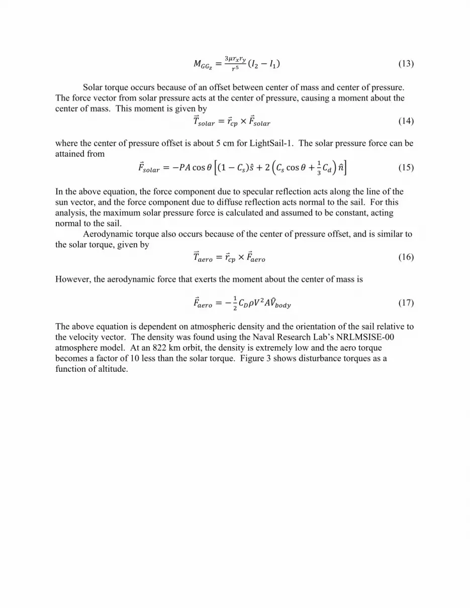
Solar torque occurs because of an offset between center of mass and center of pressure. The force vector from solar pressure acts at the center of pressure, causing a moment about the center of mass. This moment is given by (14) where the center of pressure offset is about 5 cm for LightSail-1. The solar pressure force can be attained from

cos 1 ̂ 2 cos (15)

In the above equation, the force component due to specular reflection acts along the line of the sun vector, and the force component due to diffuse reflection acts normal to the sail. For this analysis, the maximum solar pressure force is calculated and assumed to be constant, acting normal to the sail. Aerodynamic torque also occurs because of the center of pressure offset, and is similar to the solar torque, given by (16) However, the aerodynamic force that exerts the moment about the center of mass is

(17)

The above equation is dependent on atmospheric density and the orientation of the sail relative to the velocity vector. The density was found using the Naval Research Lab’s NRLMSISE-00 atmosphere model. At an 822 km orbit, the density is extremely low and the aero torque becomes a factor of 10 less than the solar torque. Figure 3 shows disturbance torques as a function of altitude.

Figure 3: Plot of disturbance torques as a function of altitude

The plot assumes the worst case torques, i.e. the sail is normal to the sun for solar torque and the sail is normal the velocity vector for aerodynamic drag. Although the gravity gradient appears constant, it actually decreases slightly with increasing altitude. Sensor Accuracy The magnetometers will be calibrated on the ground, but their sensor noise must still be taken into account in the simulations. To simulate magnetometer noise, an error term is added to the magnetic field at each point. The error term is produced with a random number generator that returns random numbers with a standard deviation of one. This number is multiplied by the expected standard deviation of the noise, which was found via testing at Cal Poly. After noise is added to the magnetic field value, the number is rounded to the nearest bit value to account for digital sensor resolution. The sun sensor accuracy is calculated the same way, except the company provided an expected accuracy that was plugged in directly to the simulation. The rate gyroscope’s behavior is more complicated to model than the sun sensors and magnetometers. In addition to noise and resolution, bias and bias stability must be accounted for in the simulation. Bias can be subtracted out after testing, but bias stability results in the gyro bias not being constant. At this point in the LightSail-1 project, bias stability is still being characterized through bench tests, so for this analysis, a conservative estimate for bias stability is used based on the data sheet for the gyros.

III. ADCS MODES

LightSail-1’s unique control system has multiple control modes that make use of different types of control. Depending on the control mode, the spacecraft will utilize pure magnetic control, magnetic control with the aid of rate gyroscopes, and control via a momentum wheel. Detumble

When the spacecraft is ejected from the P-POD, it will have an initial spin rate that should not exceed 7 deg/sec. This spin must be damped out before any active control can begin. The B-dot law, a purely magnetic control scheme, will be used to detumble the spacecraft. This method applies a magnetic dipole via the magnetorquers in the direction opposite to the change in magnetic field. The change in magnetic field is estimated by magnetometer readings spaced 10 seconds apart. The magnetorquers then apply a torque according to the equation,

       for 1,2,3 (18) This algorithm minimizes the change in magnetic field over time causing the spacecraft to align with the local magnetic field, effectively damping rotation. Momentum Wheel Spin-up

LightSail-1 will implement a momentum wheel to assist in the control of the spacecraft. The wheel serves two purposes: it will add stiffness to the system and it will be the primary actuator in the orbit raising mode which will be discussed later. During the active control modes, if the dipole produced by the magnetorquers is close to parallel with the local magnetic field, LightSail-1 will have limited control authority. In this orientation, the momentum wheel will provide stiffness in the X and Z directions, preventing the spacecraft from severely drifting away from its desired attitude.

The wheel will be off in the beginning of the mission and will remain off until after the detumble mode. When the wheel is spun up on orbit, it will impart and estimated 2.5 deg/sec angular velocity on the spacecraft, thus requiring a second B-dot mode to de-spin the spacecraft.

Sun-Pointing To demonstrate thrust via solar pressure, LightSail-1 must be capable of pointing its solar sail normal to the sun vector. In sun-pointing mode, the +Z-axis points towards the sun; this orientation defines the pointing error angle as the angle between the +Z-axis and the sun vector in body coordinates. In order to build the sun vector, there will be four sun sensors, one on each panel, as shown in figure 4 (for clarity, only two sun sensors are shown).

The paneconfigurasail. Witpanels, w

Tuses feedsun-point

Figure

els deploy toation where th this config

while still allTo achieve sudback from sting control

e 4: Illustratio

o an angle of the edges ofguration, theowing Lightun-pointing, sun sensors asystem.

Figure 5:

on of sun senso

f 165° and thf the fields oe sun sensorstSail-1 full hLightSail-1

and rate gyro

Control block

or placement

he sun sensorf view of thes will not seehemispherica

will utilize oscopes. Fig

k diagram for

and sun senso

r field of viee sun sensore any reflectal coverage.a position-pgure 5 shows

sun-pointing

or field of view

ew is 150°, crs line up partion from the

lus-rate styles a block dia

mode

ws

creating a rallel to the se sail or the

e control lawagram for the

solar

w that e

The system cycle time for the sun-pointing control mode will be similar to the B-dot timing. The system will feedback sun sensor and gyroscope data to the processor every 10 seconds. With the new feedback, the controller will solve for a new control torque to be applied by the magnetorquers for the next 10 seconds. The desired control torque will be provided by the control law, req        for  1,2,3 (19)

where Kp and Kd are system gains, ωe is the body spin rate measured by the rate gyroscopes, and θe is the pointing error angle broken down into components. As mentioned previously, theta is a function of the +Z-axis and the sun vector in body coordinates obtained from

cos · 0  0  1 T (20)

The theta vector is an eigenaxis/eigenangle control approach where the eigenaxis is given as 0  0  1 T (21) The torque generated by the control law is a requested torque; the actual control torque applied to the system is a function of the dipole produced by the magnetorquers and the magnetic field, req (22) In order to solve for the dipole necessary to produce a torque that is as close to the requested torque as possible, the following equation will be used.

reqreq (23)

This equation identifies the most efficient dipole because it allows for torque only in a direction perpendicular to the magnetic field. Orbit Raising Aside from measuring thrust, raising the orbit is the ultimate goal of the LightSail-1 mission. To accomplish this task, the spacecraft will have two main orientations. During the first half of the orbit, the spacecraft must be oriented such that the solar sail is parallel to the sun to minimize energy loss due to solar pressure. Then, in the second half of the orbit, the sail must be positioned normal to the sun in order to increase orbit energy. Figure 6 demonstrates this orbit raising technique.

Figure 6: Illustration of orbit raising mode As shown in the figure, the orbit raising scheme depends on two 90° slew maneuvers twice per orbit. The momentum wheel will be used for these maneuvers because it can slew the sail 90° in approximately 4 minutes, whereas the magnetorquers would take roughly a half hour to complete the slew maneuver. In order for the wheel to slew 90°, it will change its constant spin rate to a slightly different constant spin rate. This change will impart a spin about the Y-axis. Once the spacecraft has reached the end of the slew, the wheel will return to its original spin rate, effectively stopping the rotation and ending the slew maneuver.

IV. RESULTS

The first ADCS mode simulated was the B-dot algorithm. As shown in figure 7, the torquers damp out the body rates in about 90 minutes, roughly one orbit.

Figure 7: B-dot detumble results for the stowed configuration with wheel off

Once the wheel is spun up and sail deployed, B-dot is run again with different gains and still successfully de-spins the spacecraft, as shown in figure 8.

Figure 8: B-dot detumble results for the deployed configuration with wheel on

In this case, the expected initial body rates are slightly less than the expected body rates leaving the P-POD, but the spacecraft’s inertias are larger so the body rates are damped out in 85 minutes. This plot illustrates the dynamic coupling between in the X and Z-axes due to the presence of the momentum wheel in the Y-axis. With the ability to successfully detumble in both configurations, it is safe to begin the sun-pointing mode which requires low body rates. The sun-pointing simulation is run with the sail deployed and the wheel on. Figure 9 is an example of a sun-pointing simulation with a random initial orientation. Gray shaded areas are eclipses.

Figure 9: Plot of pointing error with random initial conditions

The random initial orientation has a 90° pointing error. This is assumed to be the worst initial condition for the sun-pointing algorithm because if the initial pointing error is more than 90 deg, the sail is flipped around with the sun on the wrong side of the sail. This condition will be sensed by the solar panels on the back of the spacecraft. If this case arises, torque about either the X or Y-axis will flip the spacecraft around so that the sun is in view of the sun sensors and the sun pointing algorithm can commence. Once LightSail-1 has successfully achieved sun-pointing, the orbit raising mode may begin. The 90° slew maneuver will be accomplished solely by changing the wheel speed. During the slew, the magnetorquers will not be active unless precession damping is necessary. The nominal wheel speed is 6500 RPM; to initiate the maneuver, the wheel speed will be changed by 1000 RPM which will cause the spacecraft to rotate at a constant rate about the Y-axis. When the slew is complete, the wheel will return to nominal speed and the spacecraft will stop rotating. At this point, the sun-pointing control system will takeover to keep the spacecraft in the correct orientation. Figure 10 demonstrates the two slews per orbit, with one of the two occurring in eclipse.

Figure 10: Demonstration of successful orbit raising maneuvers

This plot shows the sun pointing error between the +Z-axis and the sun vector in body coordinates, so each time the spacecraft points the sail parallel to the sun, the pointing error should be 90°. Also, the slew is not autonomous; it does not stop once the sun sensors read the correct angle. Instead, the slew is timed, and hand calculations were used to predict how long it would take the sail to slew 90 deg for a 1000 RPM change in wheel speed. The calculations resulted in a slew time of four minutes, and when four minutes was plugged into the simulation, the sail slewed exactly as predicted. Furthermore, angular velocity hand calculations were used to predict angular velocities in the simulation. Figure 11 is a plot of angular rates.

Figure 11: Plot of angular rates during orbit raising mode

For each slew, one can see the change in velocity about the Y-axis. The magnitude of the Y-axis velocity matches the initial hand calculations nicely.

V. CONCLUSION

This paper introduced the LightSail-1 spacecraft as well as its control system. The different ADCS modes were presented to give an understanding about how the spacecraft will control sail pointing throughout the mission. Results from the MatLab simulations were displayed, demonstrating successful fulfillment of the two main ADCS requirements: 10° pointing accuracy and orbit raising. Assumptions and limitations of this computer model were discussed. Although the simulations show that the 10°pointing accuracy and orbit raising requirements will be met, there is still testing and verification work to be done. The next step for the LightSail-1 team is to perform a processor in the loop test where the flight processor will interface with the MatLab simulation and provide the control algorithm and commands to be fed back to the simulation. Once an engineering model of the spacecraft is built, the team will perform hardware in the loop tests, so that all ADCS hardware may be validated.

REFERENCES

1. Wie, B., “Dynamic Modeling and Attitude Control of Solar Sail Spacecraft,” AIAA Paper 2002-4573, AIAA Guidance, Navigation, and, Control Conference, Monterey, CA, August 5-8, 2002. 2. Wie, B., Space Vehicle Dynamics and Control, AIAA Education Series, AIAA, Washington, DC, 1998 3. Wertz, J., Spacecraft Attitude Determination and Control, Kluwer Academic Publishers, Boston, MA, 1978. 4. Sedlund, C., “A Simple Sun-Pointing Magnetic Controller for Satellites in Equatorial Orbits,” IEEE Paper 1502, December 18, 2008. 5. Guerrant, D., Design and Analysis of Fully Magnetic Control for Picosatellite Stabilization, Master’s Thesis, California Polytechnic State University, San Luis Obispo, CA, June 2005.