NBER WORKING PAPER SERIES

INFLATION AND THE PRICE OF REAL ASSETS

Matteo LeombroniMonika PiazzesiMartin Schneider

Ciaran Rogers

Working Paper 26740http://www.nber.org/papers/w26740

NATIONAL BUREAU OF ECONOMIC RESEARCH1050 Massachusetts Avenue

Cambridge, MA 02138February 2020

For comments and suggestions, we thank Joao Cocco, Jesus Fernandez-Villaverde, John Heaton, Susan Hume McIntosh, Larry Jones, Patrick Kehoe, Per Krusell, Ricardo Lagos, Ellen McGrattan, Toby Moskowitz, Neng Wang, and many seminar and conference participants. The views expressed herein are those of the authors and do not necessarily reflect the views of the National Bureau of Economic Research.

NBER working papers are circulated for discussion and comment purposes. They have not been peer-reviewed or been subject to the review by the NBER Board of Directors that accompanies official NBER publications.

© 2020 by Matteo Leombroni, Monika Piazzesi, Martin Schneider, and Ciaran Rogers. All rights reserved. Short sections of text, not to exceed two paragraphs, may be quoted without explicit permission provided that full credit, including © notice, is given to the source.

Inflation and the Price of Real AssetsMatteo Leombroni, Monika Piazzesi, Martin Schneider, and Ciaran RogersNBER Working Paper No. 26740February 2020JEL No. E1,E2,E3,E44,G1,G11,G12,G5

ABSTRACT

In the 1970s, U.S. asset markets witnessed (i) a 25% dip in the ratio of aggregate household wealth relative to GDP and (ii) negative comovement of house and stock prices that drove a 20% portfolio shift out of equity into real estate. This study uses an overlapping generations model with uninsurable nominal risk to quantify the role of structural change in these events. We attribute the dip in wealth to the entry of baby boomers into asset markets, and to the erosion of bond portfolios by surprise inflation, both of which lowered the overall propensity to save. We also show that the Great Inflation led to a portfolio shift by making housing more attractive than equity. Disagreement about inflation across age groups matters for the size of tax effects, the volume of nominal credit, and the price of housing as collateral.

Matteo LeombroniDepartment of Economics Stanford University 579 Jane Stanford WayStanford, CA 94305-6072leombm@stanford.edu

Monika PiazzesiDepartment of EconomicsStanford University579 Jane Stanford WayStanford, CA 94305-6072and NBERpiazzesi@stanford.edu

Martin SchneiderDepartment of EconomicsStanford University579 Jane Stanford WayStanford, CA 94305-6072and NBERschneidr@stanford.edu

Ciaran RogersDepartment of Economics Stanford University 579 Jane Stanford Way Stanford, CA 94305-6072ciaran@stanford.edu

I Introduction

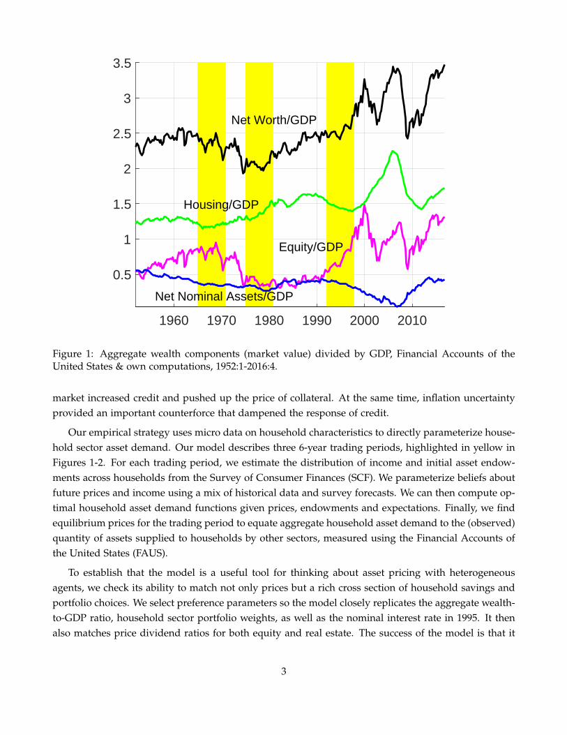
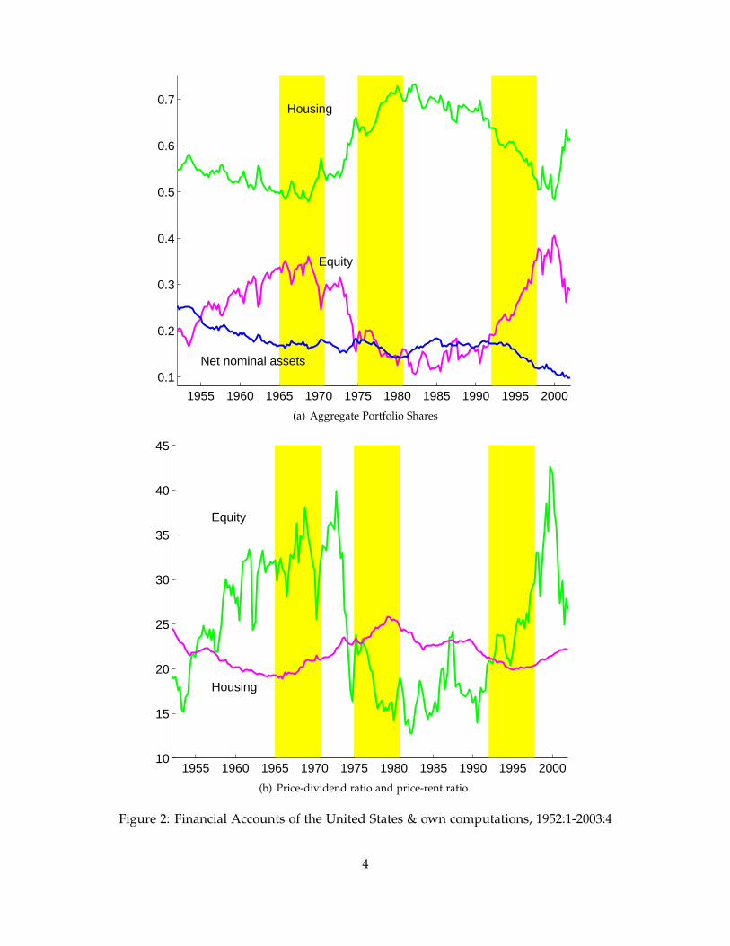
The 1970s brought dramatic changes in the size and composition of US household sector wealth. Figure1 plots key household sector positions over the postwar period. During the 1970s, household net worthas a fraction of GDP fell by 25%, before recovering again to its late 1960s value. Figure 2 zooms in onthis era and shows portfolio weights in Panel (a), in particular a 20pp shift away from equity and intoreal estate during. This portfolio adjustment was largely driven by negative comovement of asset prices– house prices rose while equity prices fell, as shown in Panel (b). Compared to the big swings in themajor real asset positions, households’ net position in nominal credit instruments was relatively stable.As documented below, the stability of net positions masks substantial increases in gross borrowing andlending within the household sector.

This paper studies the turbulence of the 1970s using an asset pricing model with heterogenousagents and incomplete markets. We consider overlapping generations of households who invest inequity and housing and who borrow and lend in nominal credit instruments. We fit the model to microdata on US households’ income and portfolio positions and then perform counterfactuals to understandthe 1970s. We attribute the wide swings in asset prices – and thereby household wealth – to two eventsunique to that decade: the entry of the young baby boomers into asset markets and the Great Inflationthat altered the distribution of real returns on credit for nominal borrowers and lenders. We showhow those events contribute to a lower average savings rate as well as a portfolio shift towards housingfor the aggregate household sector. At the same time, the outstanding quantity of houses, equity andgovernment debt declined only slightly; shifts in household asset demand thus resulted in large priceadjustments.

Individual asset demand in our model comes from a life cycle consumption savings problem withuninsurable income risk and portfolio choice between housing, equity and nominal bonds. Householdscan borrow only against housing, not against equity or human wealth (that is, permanent income).This feature helps to match that (i) many households have a lot debt, but positive net worth and (ii)younger and poorer households who have low financial wealth relative to permanent income saveless out of financial wealth. We further work with a standard income process: most income riskis idiosyncratic so human wealth is not very exposed to aggregate shocks moving house and stockprices. This feature helps match observed portfolio choice: younger households build riskier financialportfolios, in particular through leveraged investment in housing. This is optimal because they haverelatively more human wealth that is not exposed to asset price movements.

Our asset pricing results reflect how demographics and the Great Inflation altered both savings andportfolio choice. First, savings declined because there were relatively more young households, andbecause surprise inflation eroded the financial wealth of nominal lenders. Second, beliefs about futureinflation induced a portfolio shift towards housing. A prominent reason is that nominal rigidities inthe tax code favor housing over equity in times of high expected inflation. Moreover, survey data showthat households disagreed about expected inflation: young borrowers expected higher inflation – andhence lower real interest rates – than old lenders. The resulting gains from trade in the nominal credit

2

1960 1970 1980 1990 2000 2010

0.5

1

1.5

2

2.5

3

3.5

Net Worth/GDP

Housing/GDP

Equity/GDP

Net Nominal Assets/GDP

Figure 1: Aggregate wealth components (market value) divided by GDP, Financial Accounts of theUnited States & own computations, 1952:1-2016:4.

market increased credit and pushed up the price of collateral. At the same time, inflation uncertaintyprovided an important counterforce that dampened the response of credit.

Our empirical strategy uses micro data on household characteristics to directly parameterize house-hold sector asset demand. Our model describes three 6-year trading periods, highlighted in yellow inFigures 1-2. For each trading period, we estimate the distribution of income and initial asset endow-ments across households from the Survey of Consumer Finances (SCF). We parameterize beliefs aboutfuture prices and income using a mix of historical data and survey forecasts. We can then compute op-timal household asset demand functions given prices, endowments and expectations. Finally, we findequilibrium prices for the trading period to equate aggregate household asset demand to the (observed)quantity of assets supplied to households by other sectors, measured using the Financial Accounts ofthe United States (FAUS).

To establish that the model is a useful tool for thinking about asset pricing with heterogeneousagents, we check its ability to match not only prices but a rich cross section of household savings andportfolio choices. We select preference parameters so the model closely replicates the aggregate wealth-to-GDP ratio, household sector portfolio weights, as well as the nominal interest rate in 1995. It thenalso matches price dividend ratios for both equity and real estate. The success of the model is that it

3

1955 1960 1965 1970 1975 1980 1985 1990 1995 2000

0.1

0.2

0.3

0.4

0.5

0.6

0.7Housing

Equity

Net nominal assets

(a) Aggregate Portfolio Shares

1955 1960 1965 1970 1975 1980 1985 1990 1995 200010

15

20

25

30

35

40

45

Equity

Housing

(b) Price-dividend ratio and price-rent ratio

Figure 2: Financial Accounts of the United States & own computations, 1952:1-2003:4

4

captures a number of (untargeted) stylized facts about the cross-section of households in the 1995 SCF.In particular, it generates hump-shaped cohort market shares in wealth, real estate and equity, as wellas net nominal positions that increase – and real estate shares that decrease – with age and net worth.The main mechanism behind these facts is that agents who expect more future non-asset income arewilling to build more risky portfolios.

Counterfactuals that vary endowments, supply or expectations then serve to show the quantitativeimportance of each element for price fluctuations. In particular, we use the model to examine the1970s. We first show that it produces a drop in aggregate wealth between 1968 and 1978 for a widerange of expectation scenarios. It attributes the dip in the wealth-GDP ratio to two effects. First, theentry of baby boomers into asset markets lowered the average savings rate. Second, capital losses fromrealized inflation lowered wealth and hence savings, especially for older households. At the same time,lower savings were not counteracted by a large increase in interest rates, because the outside supply ofbonds to the household sector also fell – the main force here is a reduction of government debt. Here,measurement of asset supply is crucial for the quantitative results.

Our quantitative analysis implies that both inflation expectations and inflation uncertainty wererelevant for asset prices and household positions in the 1970s, while neither can account for the databy itself. When we simply endow agents with cohort median inflation expectations from the MichiganSurvey, our model predicts a portfolio shift towards housing very close to what we see in the data.However, it also generates counterfactually high credit volumes and nominal interest rate. Inflationuncertainty is a plausible feature of beliefs that makes trading in nominal credit less attractive. Ourpreferred specification for beliefs combines the two forces to account jointly for household wealth,portfolio weights, credit volumes and prices.

Our methodological approach differs from other studies of asset pricing with heterogeneous agentsand may be interesting in its own right. Our goal is to characterize asset prices that are consistent withhousehold optimization. We share this goal with conventional analysis of Euler equations pioneered byHansen and Singleton (1982) that relates asset prices to the dynamics of consumption. The differenceis that we relate asset prices to the distribution of household characteristics and the supply from othersectors, trading period by trading period. However, like Hansen and Singleton, we examine a set ofrelationships between observables that must hold in general equilibrium as long as households solveour life cycle problem. Our theory thus has content even if we do not take a stand on the behavior ofother sectors, such as the government, businesses and the rest of the world, much like Euler equationtests have content even if the dynamics of consumption are taken from the data.

A novel feature of our approach is that the distribution of the key endogenous state variable thatdrives individual savings and portfolio choice – financial wealth relative to permanent income – comesdirectly from the data. We can thus provide a new perspective on the role of heterogeneity for assetprices. Existing studies have shown that heterogeneity does not matter if asset demand functionsare approximately linear over the support of a model-implied wealth distribution. We examine assetdemand in the support of the observed wealth distribution. We find that while approximate aggregation

5

obtains within all but the youngest age cohorts, the distribution of wealth across cohorts matters a lot,as emphasized by Krueger and Kubler (2004).

The idea that demographics should matter for asset prices in theory has been discussed for a longtime, although there is no consensus on its quantitative impact. Several studies have shown that de-mographics cannot fully account for changes in stock prices if equity is the only long-lived asset in themodel (Abel, 2003, Geanakoplos, Magill and Quinzii, 2004). The effect of demographics on house priceshas been explored by Mankiw and Weil (1989) as well as Ortalo-Magne and Rady (2006). A recent lit-erature on the Great Stagnation argues that low real interest rates reflect the aging of baby boomers(for example, Gagnon, Johannsen and Lopez-Salido, 2016, or Eggertsson, Mehrotra and Robbins, 2019).These studies model the savings margin and the relationship between growth and real interest rates.Our focus is on portfolio choice and asset price fluctuations in a world with multiple long-lived assetsthat incur capital gains and losses.1 With both equity and real estate present in nonzero net supply,demographic shifts impact aggregate savings and hence the wealth-GDP ratio, but they cannot accountfor the larger movements in the individual components of wealth, especially equity.

The effects of inflation on (real) asset prices is also a familiar theme in the literature. We buildon earlier work that has stressed the interaction of taxes and inflation, in particular, Feldstein (1980),Summers (1981) and Poterba (1991). We evaluate the role of nominal rigidities in the tax code ina life cycle setup when agents disagree about inflation. Our assumptions on disagreement by ageare consistent with Malmendier and Nagel (2016) who attribute it to households’ updating beliefs overtheir lifetime. We show that disagreement interacts importantly with taxes: the fact that old householdswho hold most equity expected lower inflation reduces the strength of tax-driven portfolio shifts. Wefurther emphasize that disagreement and inflation uncertainty have opposite effects on nominal creditvolumes. The role of inflation uncertainty in the 1970s has been emphasized by Cogley and Sargent(2001).

There is a large body of work on quantitative asset pricing models with heterogeneous agents andincomplete markets. Its main focus is the properties of equity and bond returns in stationary ratio-nal expectations equilibria with real shocks, following the classic contributions of Constantinides andDuffie (1996), Heaton and Lucas (1996), and Krusell and Smith (1998). Constantinides et al. (2002), andStoresletten, Telmer and Yaron (2007) consider OLG models with equity, riskless bonds and uninsurableincome risk. Favilukis, Ludvigson and van Nieuwerburgh (2017) also allow for housing in a productioneconomy. Chien, Cole and Lustig (2012, 2016) study models with different perceptions and constraints,and hence disagreement about asset payoffs. We share with this literature the theme that movementsof the wealth distribution can matter for prices, as the identity of the average investor changes. Ourapproach of measuring that distribution directly clarifies the strength of this mechanism. We furtherdiffer from this literature in our focus on the 1970s and the unique events that shaped it.

A recent literature studies the boom-bust episodes of the 2000s (see Piazzesi and Schneider, 2016 for1Portfolio choice with housing has been considered by Flavin and Yamashita (2002), Campbell and Cocco (2003), and

Fernandez-Villaverde and Krueger (2011) Cocco (2005) and Yao and Zhang (2005) study intertemporal choice problems withthree assets that are similar to the problem solved by our households.

6

a survey). Emphasis on high frequency price changes and housing policy leads many of these studiesto introduce details of housing and mortgage markets, such as transaction costs, long term contracts,housing tenure, and heterogeneity of the housing stock. Our focus is different: since we want to studylow frequency changes in asset allocation, our model is simpler along those dimensions, but explicitlyincorporates portfolio choice between equity, housing, and risky nominal credit. Another shared themewith the literature is the supply of assets to the household sector. Justiniano, Primiceri and Tambalotti(2019) have shown that an increase in credit supply played an important role for interest rates andhouse prices in the early 2000s. We show that the stability of housing and equity supply together withthe decline in bond supply generated a large role for demand shifters.

The rest of the paper is organized as follows. Section II presents the model. Section III describesthe quantitative implementation and documents properties of the model inputs, that is, the joint dis-tribution of asset endowments and income as well as asset supply. Section IV derives predictions foroptimal household behavior and compares them to the data. Section V provides intuition for price de-termination and the role of heterogeneity for aggregates. Section VI derives predictions under baselineexpectations and shows that they help understand the evolution of the wealth-GDP ratio. Section VIIconsiders the effect of inflation on portfolio composition in the 1970s.

II Model

The model describes the household sector’s planning and asset trading in a single time period t.

A. Households

Households enter the period with assets and debt accumulated earlier. During the period, they earnlabor income, pay taxes, consume and buy assets. Labor income is affected by idiosyncratic incomeshocks. Households can invest in three types of assets: long-lived equity and real estate as well asshort-lived nominal bonds. Households face two types of aggregate risk. They face aggregate growthrisk through stock dividends and the aggregate components of their housing dividends and laborincome. They also face aggregate inflation risk when borrowing or lending because there is no risk-free asset in real terms. Households also face idiosyncratic risk which affects the return on individualhouses and labor income streams. There are only three assets, so markets are incomplete.

Planning Horizon

Consumers alive at time t differ by endowment of assets and numeraire good as well as by age.Differences in age are represented by age-specific planning horizons T and age-specific survival proba-bilities for the next period. We now describe the problem of a typical consumer with a planning horizonT > 0.

Preferences

Consumers care about two goods, housing services and other (non-housing) consumption whichserves as the numeraire. A consumption bundle of st units of housing services and ct units of numeraire

7

yields utility

(1) Ct = cδt s1−δ

t .

Preferences over (random) streams of consumption bundles {Ct} are represented by the recursive utilityspecification of Epstein and Zin (1989). Utility at time t is defined as

(2) Ut =

(C1−1/σ

t + βEt

[U1−γ

t+1

] 1−1/σ1−γ

) 11−1/σ

,

where Ut+T = Ct+T. Here σ is the intertemporal elasticity of substitution, γ is the coefficient of relativerisk aversion towards timeless gambles and β is the discount factor. The expectation operator takes intoaccount that the agent will reach the next period only with an age-specific survival probability.

Equity

Shares of equity can be thought of as trees that yield some quantity of numeraire good as dividend.A consumer enters period t with an endowment of θe

t ≥ 0 units of trees. Trees trade in the equitymarket at the ex-dividend price pe

t ; they cannot be sold short. A tree pays det units of dividend at date

t. We summarize consumers’ expectations about prices and dividends beyond period t by specifyingexpectations about returns. In particular, we assume that consumers expect to earn a (random) realreturn Re

τ+1 by holding equity between any two periods τ and τ + 1, where τ ≥ t.

Real Estate

Real estate – or houses – may be thought of as trees that yield housing services. A consumer entersperiod t with an endowment of θh

t ≥ 0 units of houses. Houses trade at the ex-dividend price pht ;

they cannot be sold short. To fix units, we assume that one unit of real estate (also referred to as onehouse) yields one unit of housing services at date t. There is a perfect rental market, where housingservices can be rented at the price ps

t . Moreover, every house requires a maintenance cost of m units ofnumeraire. If a consumer buys one unit of real estate, he obtains a dividend dh

t := pst −m. Consumers

form expectations about future returns on housing and rental prices{

Rhτ, ps

τ

}τ>t.

Borrowing and Lending

Consumers can borrow or lend by buying or selling one period discount nominal bonds. A con-sumer enters period t with an endowment of bt units of numeraire that is due to past borrowing andlending in the credit market. In particular, bt is negative if the consumer has been a net borrower inthe past. In period t, the consumer can buy or sell bonds at a price qt. A consumer expects every bondbought to pay 1/πt+1 units of the numeraire in period t + 1. Here πt+1 is random and may be thoughtof as the expected change in the dollar price of numeraire. This is a simple way to capture that debtis typically denominated in dollars.2 For every bond sold, the consumer expects to repay (1 + ξ)/πt+1

2To see why, consider a nominal bond which costs qt dollars today and pays of $1 tomorrow, or 1/pct+1 units of numeraire

consumption. Now consider a portfolio of pct nominal bonds. The price of the portfolio is qt units of numeraire and its payoff

is pct /pc

t+1 = 1/πt+1 units of numeraire tomorrow. The model thus determines the price qt of a nominal bond in dollars.

8

units of numeraire in period t+ 1, where ξ > 0 is an exogenous credit spread.3 Bond sellers – borrowers– face a collateral constraint: the value of bonds sold may not exceed a fraction φ of the value of all realestate owned by the consumer. For periods τ > t, consumers form expectations about the (random)real return on bonds

{Rb

τ

}τ>t, where Rb

τ = 1/qτ−1πτ is the (ex post) real lending rate, and Rbτ(1 + ξ) is

the (ex post) real borrowing rate.

Non-Asset Income

Consumers are endowed with an age-dependent stream of numeraire good {yτ}t+Tτ=t . Here income

should be interpreted as the sum of labor income, transfer income, and income on illiquid assets suchas private businesses.

Budget Set

The consumer enters period t with an endowment of houses and equity(θh

t , θet)

as well as anendowment of yt + bt from non-asset income and past credit market activity. At period t prices, initialwealth is therefore

(3) wt = (pht + dh

t )θht + (pe

t + det) θe

t + bt + yt.

To allocate this initial wealth to consumption and purchases of assets, the consumer chooses a planat =

{ct, st, θh

t , θet , b+t , b−t

}, where b+t ≥ 0 and b−t ≥ 0 denote the amount of bonds bought and sold,

respectively. It never makes sense for a consumer to borrow and lend simultaneously, that is, b+t > 0implies b−t = 0 and vice versa.

The plan at must satisfy the collateral constraint qtb−t ≤ φpht θh

t . The plan must also satisfy thebudget constraint

(4) ct + pst st + wt = wt,

where terminal wealth is defined as

wt = pht θh

t + pet θ

et + qtb+t − qtb−t .

To formulate the budget constraint for periods beyond t, it is helpful to define the value of theconsumer’s stock portfolio in t by we

t = pet θ

et , the consumer’s real estate portfolio by wh

t = pht θh

t aswell as the values of a (positive or negative) bond portfolio, wb+

t = qtb+t and wb−t = qtb−t . For periods

τ > t, the consumer chooses plans aτ = {cτ, sτ, whτ, we

τ, wb+τ , wb−

τ } subject to the collateral constraint

3One way to think about the organization of the credit market is that there is a financial intermediary that matches buyersand sellers in period t. In period t + 1, the intermediary will collect (1 + ξ) /πt+1 units of numeraire from every borrower(bond seller), but pay only 1/πt+1 to every lender (bond buyer), keeping ξ/πt+1 for itself. We do not model the financialintermediary explicitly since we only clear markets in period t.

9

wb−τ ≤ φwh

τ and the budget constraint

cτ + psτsτ + wh

τ + weτ + wb+

τ − wb−τ

= Rhτwh

τ−1 + Reτwe

τ−1 + Rbτwb+

τ−1 − Rbτ (1 + ξ)wb−

τ−1 + yτ.(5)

We denote the consumer’s overall plan by a =(

at, {aτ}t+Tτ=t+1

). This plan is selected to maximize utility

(2) subject to the budget constraints (3)-(5) and the collateral constraints.

Taxes

In some of our examples below, we will assume proportional income taxes as well as capital gainsand dividend taxes. This will not change the structure of the consumer’s problem, just the interpreta-tion of the symbols. In particular, labor income, dividends and returns will have to be interpreted astheir after-tax counterparts. We will discuss their precise form in the calibration section below.

Terminal Consumers

The consumers described so far have planning horizons T > 0. We also allow consumers withplanning horizon T = 0. These consumers also enter period t with asset and numeraire endowmentsthat provide them with initial wealth wt, as in (3). However, they do not make any savings or portfoliodecisions. Instead, they simply purchase numeraire and housing services in period t to maximize (1)subject to the budget constraint

ct + pst st = wt.

B. Equilibrium

To capture consumer heterogeneity, we assume a finite number of consumer types, indexed by i, withdifferent initial endowment vectors (θh

t (i) , θet (i) , yt (i) + bt (i)) and planning horizons T (i) .

New Asset Supply from the Rest of the Economy

To close the model and regulate the new supply of assets (which is exogenous to the householdsector), we introduce a rest-of-the-economy (ROE) sector. It may be thought of as a consolidation of thebusiness sector, the government and the rest of the world. The ROE sector is endowed with f e

t trees andf ht houses in period t. A positive f e

t represents the issuance of shares by the corporate sector, otherwiseshare repurchases. Similarly, a positive f h

t captures new construction of houses. In addition, the ROEenters period t with an outstanding debt of Bt units of numeraire, and it raises Dt units of numeraireby borrowing in period t. The surplus from these activities is

CROEt = f h

t (dht + ph

t ) + f et (d

et + pe

t) + Dt − Bt.

The ROE consumes the surplus CROEt . More generally, the ROE has “deep pockets” out of which it

pays for a deficit, CROEt < 0.

10

Aggregate Asset Supply

We normalize initial endowments of equity and real estate such that there is a single tree and asingle house outstanding:

∑i θht (i) = ∑i θ

et (i) = 1.

In addition, we assume that initial endowments from past credit market activity are consistent, in thesense that every position corresponds to some offsetting position, either by a household or by the ROEsector:

∑i bt (i) = Bt.

Equilibrium

An equilibrium consists of a vector of prices for period t,(

pht , pe

t , qt, pst)

, a surplus for the ROE sectorCROE

t , as well as a collection of consumer plans for period t, {at (i)} = {ct (i) , st (i), θht (i) , θe

t (i) , b+t (i) , b−t (i)}such that

(1) for every consumer, the plan at (i) is part of an optimal plan a (i) =(

at (i) , {aτ (i)}t+T(i)τ=t+1

)given

consumer i′s endowment, planning horizon, and expectations about future prices and returns;

(2) markets for all assets and goods clear:

∑iθht (i) = 1 + f h

t ,

∑iθet (i) = 1 + f e

t ,

qt∑ib+t (i) = Dt + qt∑ib

−t (i) ,

∑ict (i) + m θht (i) + CROE

t = ∑iyt (i) + det (1 + f e

t ) ,

∑ist (i) = ∑iθht (i) .

In addition to market clearing conditions for stocks, bonds and numeraire, there are two marketclearing conditions for housing: one for the asset “real estate” and one for the good “housing services”.The first equation ensures that the total demand for houses equals their total supply. The fifth equationensures that the fraction of houses that owners set aside as investment real estate – that is, sellingservices in the rental market – is the same as the fraction of housing services demanded in the rentalmarket. As is common in competitive models, one of the five market clearing conditions is redundant,as it is implied by the sum of consumers’ budget constraints, the definition of CROE

t and the other fourmarket clearing conditions. Solving for equilibrium prices thus amounts to solving a system of fourequation in the four prices ph

t , pet , qt and ps

t .

C. Discussion of the Assumptions

Connection to National Income Accounting

Introducing the ROE sector allows us to accommodate deviations between consumption and house-

11

hold sector income that are usually ignored in endowment economy models. To clarify the connectionto the FAUS/NIPA framework, we sum up the last three market clearing conditions and rearrange toobtain

∑ict (i) + pst st (i)︸ ︷︷ ︸+ f h

t pht + f e

t pet + Dt − qt−1Bt︸ ︷︷ ︸ = ∑iyt (i) + de

t + dht + (1− qt−1) Bt.︸ ︷︷ ︸

personal consumption personal savings personal income

The first term on the left-hand side of this equation is personal consumption, including housingservices. The right-hand side of this equation represents personal income. While our definition ofincome differs from the NIPAs in some details, as discussed in the next section, the basic componentsare the same: non-asset income, dividends on the two long-lived assets, and net interest. The differencebetween personal consumption and income is the second term on the left-hand side, which representspersonal savings. It consists of the same components as in the FAUS: net acquisition of real estate andnet acquisition of financial assets, here equity and bonds.4 The supply of assets provided by the ROEthus allows for positive or negative personal savings in equilibrium.

Asset Supply and Savings

The possibility of nonzero savings makes our model compatible with richer models that explicitlyconsider production, fiscal policy, and the fact that the US is not a closed economy. A richer modelwould give rise to explicit policy functions for the business, government, and foreign sectors that linkthose sectors’ net asset supplies to market prices. At the same time, if the richer model accounts forobserved supply by the ROE sector to the household sector, evaluating the policy functions at observedprices should deliver observed quantities. In our empirical implementation below, we thus set the netsupply by the ROE equal to observed quantities.

We thus determine asset prices such that households are willing to hold observed quantities, whichwould also be provided by the ROE in a richer model that fits observed quantities. When the other sideof the market is also derived from optimal policies, the household sector could be modelled in exactlythe same way as in our model.5 Our approach thus avoids a common criticism of asset pricing modelsbased on endowment economies: model features that help explain prices in an endowment economy– for example, certain preference specifications – may entail undesirable outcomes once savings areallowed. Our strategy matches simultaneously prices and observed household savings.

4FAUS savings is larger than our concept of savings because FAUS investment contains investment in noncorporate busi-ness, as well as purchases of consumer durables. In our empirical implementation, noncorporate business is treated asilliquid and investment in it is subtracted from income. In addition, we follow the NIPA convention of treating expenditureon durables as consumption. This seems appropriate given the 6-year length of each period in our model.

5Our modelling strategy requires some care in interpreting counterfactuals. For example, computing the response to achange in tax rates cannot tell us what would have happened to the economy as a whole, since we do not model supplyresponses to tax changes. Instead, the counterfactual tells us what the household sector would have done if taxes changed,and what the effect on prices would have been had supply remained unchanged. The reason the exercise is still useful is thatit allows us to see whether tax changes can play a first order role in accounting for asset prices over time, given the actualmovements in equilibrium quantities.

12

Prices vs. Quantities

It is not common in asset pricing models to distinguish asset prices and quantities. Indeed, if thedividend from a single “tree” provides all consumption, there is no meaningful concept of quantity– doubling the quantity of trees is the same as doubling the dividend on the single tree. In ourmodel, asset quantity is identified because we allow trades between the household sector and the ROE.Households increase or decrease the quantity of trees they own only through such trades. The changein quantity is determined by comparing the change in market capitalization with the capital gain onpre-existing trees. While a capital gain is enjoyed by households who enter the periods owning trees, achange in capitalization requires households to pay for new trees.

Expectations

Our approach does not place restrictions on prices beyond date t itself. In particular, it does notrequire that agents agree on a common model structure that links future fundamentals and prices. Asfar as household behavior is concerned, our empirical implementation instead follows the literatureon portfolio choice, where exogenous processes for returns and income are standard. However, wego beyond portfolio choice models in that we explore how equilibrium prices change when investors’expectations about returns vary in a controlled way. This is particularly useful if expectations arematched to inflation surveys, as we do in Section VII, since expected inflation directly affects returns.

Our model does not link price expectations to future model-implied prices. Such a connection isimposed in rational expectations models, and more generally whenever agents have “structural knowl-edge” of the price function, such as in many models with Bayesian learning. Assuming structuralknowledge has appeal when agents understand well how the economy works, for example becausethere are stable recurrent patterns in the data. Indeed, in a stationary environment, “knowing the pricefunction” can be justified by learning from past data, and appears no more restrictive than “knowingthe distribution of fundamentals”.

However, our interest in this paper is in low frequency asset-price movements during times ofstructural change. In this context, it is not clear why agent beliefs should be based on the particularmodel structure that we consider today with the benefit of hindsight. For example, it is not clearwhether household expectations should be required to anticipate structural change that we only nowknow to have taken place. Since the usual justifications for narrowing down the set of expectations byimposing rational expectations or structural knowledge is not compelling, we turn to flexible modellingof exogenous expectations.

Connection to consumption-based asset-pricing

Many studies that examine asset prices jointly with real variables focus on consumption, in partic-ular the connection between consumption and asset prices implied by intertemporal Euler equations.Since our model is based on utility maximization, an Euler equation also holds, at least at the individ-ual household level. Instead of considering a map from endowments and supply to prices, one couldconsider examining the Euler equation directly. In certain ways this might be easier, since it requires

13

only one non-price variable, consumption, although serious treatment of heterogeneous agents wouldrequire household-level consumption data.

The main problem with the Euler equation approach in our context is that the Euler equation relatesprices to investors’ planned consumption, and thus makes sense only if planned consumption can bemeasured. Imposing rational expectations effectively makes the (subjective) distribution of plannedconsumption measurable by setting it equal – by assumption – to the observed distribution of realizedconsumption. As discussed above, this is a strong assumption that is not compelling in the context ofstructural change. As a result, the Euler equation approach itself is not appealing for the applicationwe consider in this paper.

Table 1: Negative Net Worth Households

1962 SCF 1995 SCF 2001 SCFavg. 29 53 77 avg. 29 53 77 avg. 29 53 77

% of households 4% 10% 3% 2% 7% 18% 4% 2% 7% 20% 5% 2%net worth (in $) -.4K -.4K -.8K -1.3K -9K -9K -13K -8K -11K -10K -9K -1K

Note: Row 1 reports the percentage of households with negative net worth in the U.S. pop-ulation based on different SCFs. Row 2 reports the average net worth of these householdsin dollars.

Nonnegative Net Worth

Few households have negative net worth. Table 1 documents that the percentage of negative networth households has always been between 4% and 7%. Table 1 also shows that the net worth of thesehouseholds is moderate. For example, the average net worth was -11K Dollars in 2001. These numberssuggest that the most important reason for household borrowing is not consumption smoothing. In-stead, young households “borrow to gamble” — they borrow to be able to buy more risky assets, suchas housing.

The Role of Housing

In both our model and in reality, housing plays a dual role: housing can be used for consumptionand investment. In its role as a consumption good, housing is different from other consumption,because it enters the utility function separately and has a different price ps

t . In its role as asset, housingis different from other assets, because of its return properties (which will be discussed later), andbecause it can serve as collateral. In reality, the two roles are often connected, because the amountof housing services consumed is equal to the dividend paid by the amount of housing held in theportfolio. In our model, we abstract from this issue (at least for now) for several reasons. First, mosthomeowners not only own their primary residence, but also some investment real estate (such as timeshares, vacation homes, secondary homes, etc.) Hence, there is no tight link between consumption andinvestment for these households. Second, U.S. households are highly mobile. As a consequence, houses

14

are owned by the same owner on average for only seven years, which is roughly the same length as aperiod in our model. Moreover, the decision to move is often more or less exogenous to households(for example, because of job loss, divorce, death of the spouse, etc.)

III Quantitative Implementation

The inputs needed for implementing the model are (i) the joint distribution of asset endowments andincome, (ii) aggregate supply of assets to the household sector from other sectors, (iii) expectationsabout labor income and asset returns and (iv) parameter values for preferences and the credit market.We describe our choices in detail in the Appendix; here we provide a brief overview. We start with adescription of what a model period corresponds to in the data.

Timing

The length of a period is six years. Since the model compresses what happens over a six yearspan into a single date, prices and holdings are best thought of as period averages. We assume thatconsumers expect to live for at most 10 such periods, where the first period of life corresponds roughlyto the beginning of working life. In any given period, we consider 11 age groups of households (<23,24-29, 30-35, 36-41, 42-47, 48-53, 54-59, 60-65, 66-71, 72-77, >77) who make portfolio choice decisions.For ease of comparison with other models, we nevertheless report numbers at annual rates.

In the time series dimension, we focus on three six-year periods, namely 1965-70, 1975-80, and1992-97. To construct asset endowment distributions, we use data on asset holdings from the respectiveprecursor periods 1959-64, 1969-74, and 1986-91. Micro data is not available at high frequencies. Tocapture the wealth and income distribution during a period, we have chosen the above intervals so thatevery period that contains a Survey of Consumer Finances contains is in the 4th year of the period;we thus use surveys from 1962, 1989 and 1995. We use the 4th year survey to infer income and assetholdings where possible.

A. Defining Assets and Income

We map the three assets in the model to three broad asset classes in US aggregate and householdstatistics. For equity and real estate, we use the Financial Accounts of the United States (FAUS) toderive measures of (i) aggregate holdings of the household sector, (ii) net purchases by the householdsector and (iii) aggregate dividends received by the household sector. We use the numbers on value,dividends and new issues to calculate price dividend ratios and holding returns on equity and realestate. For both assets, we also define corresponding measures at the individual level using the Surveyof Consumer Finances (SCF).

Equity

We identify equity with shares in corporations held and controlled by households. We include bothpublicly traded and closely held shares, and both foreign and domestic equity. We also include sharesheld indirectly through investment intermediaries if the household can be assumed to control the asset

15

allocation (into our broad asset classes) himself. We take this to be true for mutual funds and definedcontribution (DC) pension plans. We do not include equity in defined benefit (DB) pension plans, sincehouseholds typically do not control the asset allocation of such funds. Our concept of dividends thusequals dividends received by households from the National Income and Product Accounts (NIPA) lessdividends on household holdings in DB plans.

Real estate

Our concept of residential real estate contains owner-occupied housing, directly held residential in-vestment real estate, as well as residential real estate recorded in the FAUS/NIPA as held indirectly byhouseholds through noncorporate businesses. This concept contains almost all residential real estateholdings, since very few residential properties are owned by corporations. We take housing dividendsto be housing consumption net of maintenance and property tax from NIPA. For net purchases of newhouses, we use aggregate residential investment from NIPA.

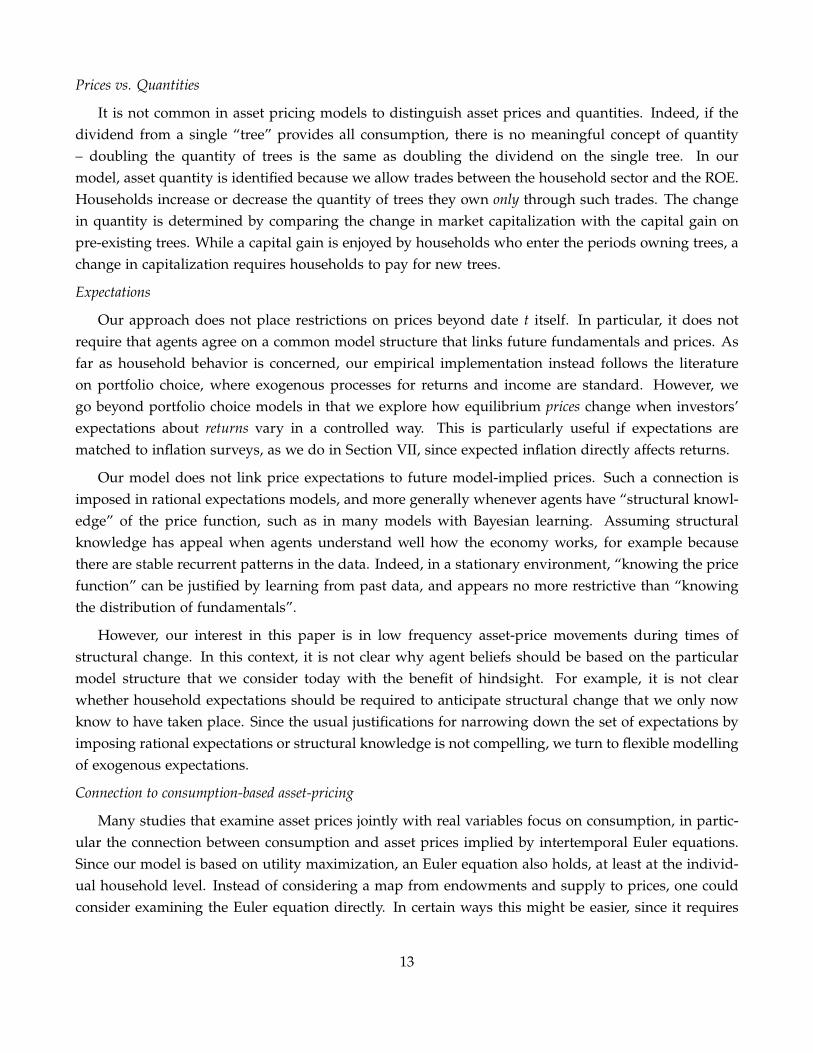
The ROE sector endowment of equity consists of net new equity purchased by the household sectorduring the trading period. The factor f e states this endowment relative to total market capitalization inthe model. We thus use net purchases of corporate equity divided by total household holdings of cor-porate equity. The ROE sector endowment of residential real estate consists of residential investment,divided by the value of residential real estate. The top panel of Figure 3 plots quarterly series for bothROE endowment, or “asset supply” numbers. The calibration of the model uses six-year averages ofthese series.

Nominal positions

Our concept for a household’s bond holdings is its net nominal position, that is, the market valueof all nominal assets minus the market value of nominal liabilities. As for equity, holdings include notonly direct holdings, but also indirect holdings through investment intermediaries. To calculate marketvalue, we use the market value adjustment factors for nominal positions in the U.S. from Doepkeand Schneider (2006). In line with our treatment of tenant-occupied real estate, we assign residentialmortgages issued by noncorporate businesses directly to households.

When considering gross nominal positions, we must take into account the fact that some netting ofpositions occurs at the individual level. A typical household will have both a mortgage loan or creditcard and a savings account or bonds in a pension fund. However, the model has only one type ofnominal asset, and a household can be either long or short that asset. If we were to match the grossaggregates from the FAUS or SCF in our model, this would inevitably lead to net positions that aretoo large. Instead, we sort SCF households into borrowers and lenders, according to whether their netnominal position is negative or not. The numbers for gross borrowing and lending are then calculatedas minus the sum of net nominal positions of borrowers as well as the sum of net positions of alllenders, respectively.

Table 2 summarizes these gross nominal positions after individual netting from the SCF and com-pares them to those in the FAUS. Both the FAUS numbers and our estimates reflect a steady increase in

16

1955 1960 1965 1970 1975 1980 1985 1990 1995 2000

−0.08

−0.06

−0.04

−0.02

0

0.02

0.04

long lived asset supply (% market cap)

housesstocks

1955 1960 1965 1970 1975 1980 1985 1990 1995 20000.3

0.35

0.4

0.45

0.5

0.55

Bond supply (% gdp)

Figure 3: Top panel: Net new corporate equity as a percent of total household holdings of corporateequity and residential investment as percent of value of residential real estate. Data are quarterly atannual rates. Bottom panel: Net nominal position of household sector as a percent of GDP.

borrowing by the household sector. At the same time, both sets of numbers show a reduction in nomi-nal asset holdings in the 1970s followed by an increase between 1978 and 1995. Throughout, individualnetting reduces gross lending by roughly one third, while it reduces gross borrowing by slightly morethan half.

Table 2: Gross Borrowing and Lending (%GDP)1968 1978 1995

lending borrowing lending borrowing lending borrowingFAUS aggregates 88 47 84 51 107 68

SCF after indiv. netting 61 20 56 23 70 31

The initial nominal position of the ROE sector is taken to be minus the aggregate (updated) netnominal position of the household sector. Finally, the new net nominal position of the ROE in period t– in other words, the “supply of bonds” to the household sector – is taken to be minus the aggregatenet nominal positions from the FAUS for period t. This series is reproduced in the bottom panel ofFigure 3.

17

Non-Asset Income

Our concept of non-asset income comprises all income that is available for consumption or invest-ment, but not received from payoffs of one of our three assets. We construct an aggregate measureof such income from NIPA and then derive a counterpart at the household level from the SCF. Of thevarious components of worker compensation, we include only wages and salaries, as well as employercontributions to DC pension plans. We do not include employer contributions to DB pension plansor health insurance, since these funds are not available for consumption or investment. However, wedo include benefits disbursed from DB plans and health plans. Also included are transfers from thegovernment. Finally, we subtract personal income tax on non-asset income.

B. The joint distribution of asset endowments and income

Consumers in our model are endowed with both assets and non-asset income. To capture decisionsmade by the cross-section of households, we thus have to initialize the model for every period t witha joint distribution of asset endowment and income. We derive this distribution from data on terminalasset holdings and income in the precursor period t− 1. To handle multidimensional distributions, weapproximate them by a finite number of household types. Types are selected to retain key moments ofthe full distribution, in particular aggregate gross borrowing and lending.

Since the aggregate endowment of long-lived assets is normalized to one, we can read off theendowment of a household type in period t from its market share in period t− 1. For each long-livedasset a = h, e, suppose that wa

t−1 (i) is the market value of investor i’s position in t− 1 in asset a. Itsinitial holdings are given by

θat (i) = θa

t−1 (i) =wa

t−1 (i)∑iwa

t−1 (i)=

pat−1 θa

t−1 (i)pa

t−1∑iθat−1 (i)

= market share of household i in period t− 1.

For nominal assets, the above approach does not work since these assets are short-term in ourmodel. Instead, we determine the market value of nominal positions in period t− 1 and update it toperiod t by multiplying it with a nominal interest rate factor:

bt (i) = (1 + it−1)wb

t−1 (i)GDPt

= (1 + it−1)wb

t−1 (i)

∑iwbt−1 (i)

∑iwbt−1 (i)

GDPt−1

GDPt−1

GDPt.

Letting gt denote real GDP growth and Dt the aggregate net nominal position as a fraction of GDP,we have

bt (i) ≈ θbt−1 (i) Dt−1 (1 + it−1 − gt − πt) .

This equation distinguishes three reasons why bt (i) might be small in a given period. The first is simply

18

that the household’s nominal investment in the previous period was small. Since all endowments arestated relative to GDP, all current initial nominal positions are also small if the economy has justundergone a period of rapid growth. Finally, initial nominal positions are affected by surprise inflationover the last few years. If the nominal interest rate it−1 does not compensate for realized inflation πt,then b

it is small (in absolute value). Surprise inflation thus increases the negative position of a borrower,

while it decreases the positive position of a borrower.

The final step in our construction of the joint income and endowment distribution is to specify themarginal distribution of non-asset income. Here we make use of the fact that income is observed inperiod t − 1 in the SCF. We then assume that the transition between t − 1 and t is determined by astochastic process for non-asset income. We employ the same process that agents in the model useto forecast their non-asset income, described in Appendix B. This approach allows us to capture thecorrelation between income and initial asset holdings that is implied by the joint distribution of incomeand wealth.

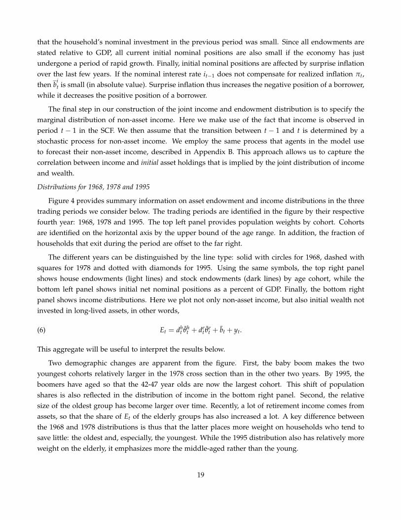
Distributions for 1968, 1978 and 1995

Figure 4 provides summary information on asset endowment and income distributions in the threetrading periods we consider below. The trading periods are identified in the figure by their respectivefourth year: 1968, 1978 and 1995. The top left panel provides population weights by cohort. Cohortsare identified on the horizontal axis by the upper bound of the age range. In addition, the fraction ofhouseholds that exit during the period are offset to the far right.

The different years can be distinguished by the line type: solid with circles for 1968, dashed withsquares for 1978 and dotted with diamonds for 1995. Using the same symbols, the top right panelshows house endowments (light lines) and stock endowments (dark lines) by age cohort, while thebottom left panel shows initial net nominal positions as a percent of GDP. Finally, the bottom rightpanel shows income distributions. Here we plot not only non-asset income, but also initial wealth notinvested in long-lived assets, in other words,

(6) Et = dht θh

t + det θ

et + bt + yt.

This aggregate will be useful to interpret the results below.

Two demographic changes are apparent from the figure. First, the baby boom makes the twoyoungest cohorts relatively larger in the 1978 cross section than in the other two years. By 1995, theboomers have aged so that the 42-47 year olds are now the largest cohort. This shift of populationshares is also reflected in the distribution of income in the bottom right panel. Second, the relativesize of the oldest group has become larger over time. Recently, a lot of retirement income comes fromassets, so that the share of Et of the elderly groups has also increased a lot. A key difference betweenthe 1968 and 1978 distributions is thus that the latter places more weight on households who tend tosave little: the oldest and, especially, the youngest. While the 1995 distribution also has relatively moreweight on the elderly, it emphasizes more the middle-aged rather than the young.

19

29 35 41 47 53 59 65 72 77 83

0.04

0.05

0.06

0.07

0.08

0.09

0.1

0.11

0.12

0.13

Population Weights

196819781995

29 35 41 47 53 59 65 72 77 830

0.02

0.04

0.06

0.08

0.1

0.12

0.14

0.16

0.18

0.2

Endowments of houses (light), stocks (dark)

29 35 41 47 53 59 65 72 77 83

−1

−0.5

0

0.5

1

1.5

2

Bond endowments (% GDP)

29 35 41 47 53 59 65 72 77 830

2

4

6

8

10

12

Income (dark) and E (light) (% GDP)

Figure 4: Asset endowment and income distributions in 1968, 1978 and 1995. Top left panel: Populationweights by cohort, identified on the horizontal axis by the upper bound of the age range. Exitinghouseholds during the period are on the far right. Top right panel: House endowments (light lines) andstock endowments (dark lines) by age cohort. Bottom left panel: initial net nominal positions as a percentof GDP. Bottom right panel: Income distributions.

The comparison of stock and house endowments in the top right panel reveals that housing is moreof an asset for younger people. For all years, the market shares of cohorts in their thirties and fortiesare larger for houses than for stocks, while the opposite is true for older cohorts. By and large, themarket shares are however quite similar across years. In contrast, the behavior of net nominal positionsrelative to GDP (bottom right hand panel) has changed markedly over time. In particular, the amountof intergenerational borrowing and lending has increased: young households today borrow relativelymore, while old households hold relatively more bonds.

20

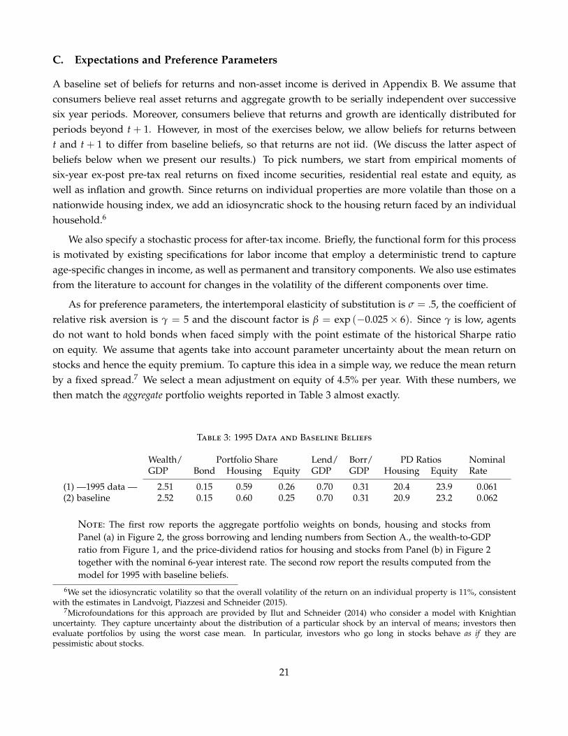
C. Expectations and Preference Parameters

A baseline set of beliefs for returns and non-asset income is derived in Appendix B. We assume thatconsumers believe real asset returns and aggregate growth to be serially independent over successivesix year periods. Moreover, consumers believe that returns and growth are identically distributed forperiods beyond t + 1. However, in most of the exercises below, we allow beliefs for returns betweent and t + 1 to differ from baseline beliefs, so that returns are not iid. (We discuss the latter aspect ofbeliefs below when we present our results.) To pick numbers, we start from empirical moments ofsix-year ex-post pre-tax real returns on fixed income securities, residential real estate and equity, aswell as inflation and growth. Since returns on individual properties are more volatile than those on anationwide housing index, we add an idiosyncratic shock to the housing return faced by an individualhousehold.6

We also specify a stochastic process for after-tax income. Briefly, the functional form for this processis motivated by existing specifications for labor income that employ a deterministic trend to captureage-specific changes in income, as well as permanent and transitory components. We also use estimatesfrom the literature to account for changes in the volatility of the different components over time.

As for preference parameters, the intertemporal elasticity of substitution is σ = .5, the coefficient ofrelative risk aversion is γ = 5 and the discount factor is β = exp (−0.025× 6). Since γ is low, agentsdo not want to hold bonds when faced simply with the point estimate of the historical Sharpe ratioon equity. We assume that agents take into account parameter uncertainty about the mean return onstocks and hence the equity premium. To capture this idea in a simple way, we reduce the mean returnby a fixed spread.7 We select a mean adjustment on equity of 4.5% per year. With these numbers, wethen match the aggregate portfolio weights reported in Table 3 almost exactly.

Table 3: 1995 Data and Baseline Beliefs

Wealth/ Portfolio Share Lend/ Borr/ PD Ratios NominalGDP Bond Housing Equity GDP GDP Housing Equity Rate

(1) —1995 data — 2.51 0.15 0.59 0.26 0.70 0.31 20.4 23.9 0.061(2) baseline 2.52 0.15 0.60 0.25 0.70 0.31 20.9 23.2 0.062

Note: The first row reports the aggregate portfolio weights on bonds, housing and stocks fromPanel (a) in Figure 2, the gross borrowing and lending numbers from Section A., the wealth-to-GDPratio from Figure 1, and the price-dividend ratios for housing and stocks from Panel (b) in Figure 2together with the nominal 6-year interest rate. The second row report the results computed from themodel for 1995 with baseline beliefs.

6We set the idiosyncratic volatility so that the overall volatility of the return on an individual property is 11%, consistentwith the estimates in Landvoigt, Piazzesi and Schneider (2015).

7Microfoundations for this approach are provided by Ilut and Schneider (2014) who consider a model with Knightianuncertainty. They capture uncertainty about the distribution of a particular shock by an interval of means; investors thenevaluate portfolios by using the worst case mean. In particular, investors who go long in stocks behave as if they arepessimistic about stocks.

21

An alternative strategy would be to work with agents who have “high aversion against low per-ceived risk.” In this case, agents base their portfolio choice on the historical variances from Table B.2,but are characterized by high risk aversion, γ = 25, and high discounting, β = exp (−0.07× 6). Thehigh γ is needed to lower the portfolio weight on bonds, while the low β is needed to reduce theprecautionary savings motive in the presence of uninsurable income shocks. While the tables belowreport results based on agents with “low aversion against high perceived risk,” we would get resultscomparable to those in Table 3 based on this alternative parametrization.8

D. Taxes and the Credit Market

It remains to select parameters to capture taxes on investment as well as consumers’ opportunities forborrowing. We set the maximal loan-to-value ratio to φ = .8., the modal value in the United States. Wefurther choose spreads between borrowing and lending rates to match aggregate gross credit volumesin the economy. For 1995, we back out a value of 1.6%, in the ball park of existing estimates. Before thederegulation of banking and the increase in securitization of the early 1980s, mortgage markets wereless developed. We back out the spread for the earlier episodes from credit volumes in 1968, and finda value of 2%.

Investors care about after-tax real returns. In particular, taxes affect the relative attractiveness ofequity and real estate. On the one hand, dividends on owner-occupied housing are directly consumedand hence not taxed, while dividends on stocks are subject to income tax. On the other hand, capitalgains on housing are more easily sheltered from taxes than capital gains on stocks. This is becausemany consumers simply live in their house for a long period of time and never realize the capitalgains. Capital gains tax matters especially in inflationary times, because the nominal gain is taxed: theeffective real after tax return on an asset subject to capital gains tax is therefore relatively lower withinflation. Inflation also increases the subsidy from mortgage deductability.

To measure the effect of capital gains taxes, one would ideally like to explicitly distinguish realizedand unrealized capital gains. However, this would involve introducing state variables to keep trackof past individual asset purchase decisions. To keep the problem manageable, we adopt a simplerapproach: we adjust our benchmark returns to capture the effects described above. For our baseline setof results, we assume proportional taxes, and we set both the capital gains tax rate and the income taxrate to 20%. This number is consistent with the numbers reported by Sialm (2009) for average effectivetax rates on equity returns as well as capital gains tax rates in the 1970s. We define after tax real stockreturns by subtracting 20% from realized net real stock returns and then further subtracting 20% timesthe realized rate of inflation to capture the fact that nominal capital gains are taxed. In contrast, weassume that returns on real estate are not taxed.

8Yet another way to obtain realistic aggregate portfolio weights is to combine low risk aversion with first-time participationcosts, as shown by Gomes and Michaelides (2005).

22

IV Household Behavior

In this section, we consider savings and portfolio choice in the cross section of households. We focuson baseline beliefs for 1995, the year we have used to calibrate beliefs. The initial distribution of assetendowments and income is derived from the 1989 SCF, as discussed in Section III. We first presentoptimal policies as functions of wealth and income. We then compare the predictions of the model forthe cross-section of households in 1995 to actual observations from the 1995 SCF.

A. Lifecycle Savings and Portfolios

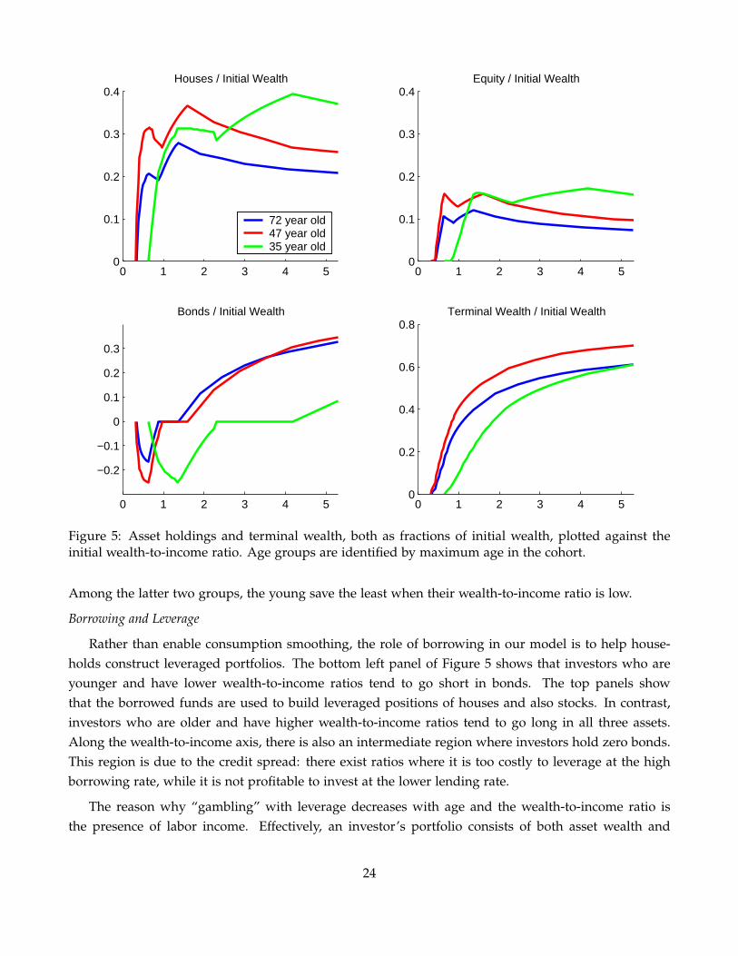
Since preferences are homothetic and all constraints are linear, the optimal savings rate and portfolioweights depend only on age and the ratio of initial wealth wt – defined in (3) above as asset wealthplus non-asset income – to the permanent component of non-asset income, say yt. For simplicity,we refer to wt/yt as the wealth-to-income ratio. Figure 5 plots agent decisions as a function of thiswealth-to-income ratio.

Savings

The bottom right panel shows the ratio wt/wt of terminal wealth to initial wealth, that is, thesavings rate out of initial wealth. Savings are always positive, since the borrowing constraint precludesstrategies that involve negative net worth. Investors who have more income in later periods than in thecurrent period thus cannot shift that income forward by borrowing. In this sense, there is no borrowingfor “consumption smoothing” purposes: all current consumption must instead come out of currentincome or from selling initial asset wealth.

If initial wealth is very low relative to income, all assets will be sold and all income consumed, sothat the investor enters the next period with zero asset wealth. As initial wealth increases, a greaterfraction of it is saved for future consumption. In the absence of labor income, our assumption of seriallyindependent returns implies a constant optimal savings rate. As wealth becomes large relative to thepermanent component of income, the savings rate converges to this constant.

The bottom right panel also illustrates how the savings rate changes with age. There are tworelevant effects. On the one hand, younger investors have a longer planning horizon and thereforetend to spread any wealth they have over more remaining periods. This effect by itself tends to makeyounger investors save more. On the other hand, the non-asset income profile is hump-shaped, sothat middle-aged investors can rely more on labor income for consumption than either young or oldinvestors. This tends to make middle-aged investors save relatively more than other investors.

The first effect dominates when labor income is not very important, that is, when the wealth-to-income ratio is high. The figure shows that at high wealth-to-income ratios, the savings rate of the29-35 year old group climbs beyond that of the oldest investor group. It eventually also climbs abovethe savings rate of the 48-53 year old group. The second effect is important for lower wealth-to-incomeratios, especially in the empirically relevant range around 1-2, where most ratios lie in the data. In thisregion, the savings rate of the middle-aged is highest, whereas both the young and the old save less.

23

0 1 2 3 4 50

0.1

0.2

0.3

0.4Houses / Initial Wealth

72 year old47 year old35 year old

0 1 2 3 4 50

0.1

0.2

0.3

0.4Equity / Initial Wealth

0 1 2 3 4 5

−0.2

−0.1

0

0.1

0.2

0.3

Bonds / Initial Wealth

0 1 2 3 4 50

0.2

0.4

0.6

0.8Terminal Wealth / Initial Wealth

Figure 5: Asset holdings and terminal wealth, both as fractions of initial wealth, plotted against theinitial wealth-to-income ratio. Age groups are identified by maximum age in the cohort.

Among the latter two groups, the young save the least when their wealth-to-income ratio is low.

Borrowing and Leverage

Rather than enable consumption smoothing, the role of borrowing in our model is to help house-holds construct leveraged portfolios. The bottom left panel of Figure 5 shows that investors who areyounger and have lower wealth-to-income ratios tend to go short in bonds. The top panels showthat the borrowed funds are used to build leveraged positions of houses and also stocks. In contrast,investors who are older and have higher wealth-to-income ratios tend to go long in all three assets.Along the wealth-to-income axis, there is also an intermediate region where investors hold zero bonds.This region is due to the credit spread: there exist ratios where it is too costly to leverage at the highborrowing rate, while it is not profitable to invest at the lower lending rate.

The reason why “gambling” with leverage decreases with age and the wealth-to-income ratio isthe presence of labor income. Effectively, an investor’s portfolio consists of both asset wealth and

24

human wealth. Younger and lower wealth-to-income households have relatively more human wealth.Moreover, the correlation of human wealth and asset wealth is small. As a result, households with alot of labor income hold riskier strategies in the asset part of their portfolios. This effect has also beenobserved by Jagannathan and Kocherlakota (1996), Heaton and Lucas (2000), and Cocco (2005).

Stock v. House Ownership

For most age groups and wealth-to-income ratios, investment in houses is larger than investment instocks. This reflects the higher Sharpe ratio of houses as well as the fact that houses serve as collateralwhile stocks do not. The latter feature also explains why the ratio of house to stock ownership isdecreasing with both age and wealth-to-income ratio: for richer and older households, leverage is lessimportant, and so the collateral value of a house is smaller.

Currently, the model cannot capture the fact that the portfolio weight on stocks tends to increasewith the wealth-to-income ratio. While it is true in the model that people with higher wealth-to-incomeown more stocks relative to housing, they also hold much more bonds relative to both of the otherassets. As a result, their overall portfolio weight on stocks actually falls with the wealth-to-incomeratio. The behavior of the portfolio weight on stocks implies that the model produces typically too littleconcentration of stock ownership.

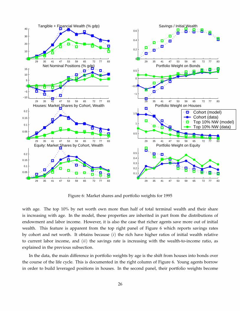
B. The Cross Section of Asset Holdings

Figure 6 plots predicted portfolio weights and market shares for various groups of households for 1995,given baseline beliefs. The panels also contain actual weights and market shares for the respectivegroups from the 1995 SCF. It is useful to compare both portfolio weights and market shares, since thelatter also require the model to do a good job on savings behavior. Indeed, defining aggregate initialwealth W = ∑iw (i), the market share of asset a = h, e for a household i can be written as

θa (i) =αa (i) w (i)

∑iαa (i) w (i)

=αa (i)

∑iαa (i) w(i)

W

w (i)W

=αa (i)

αaw (i)

W,

where αa (i) is household i’s portfolio weight and αa is the aggregate portfolio weight on asset a. Amodel that correctly predicts the cross section of portfolio shares will therefore only correctly predictthe cross section of market shares if it also captures the cross section of terminal wealth. The latter inturn depends on the savings rate of different groups of agents.

The first row of Figure 6 documents savings behavior by cohort and wealth level. The top left panelplots terminal wealth as a fraction of GDP at the cohort level (blue/black lines) for the model (dottedline) and the data (solid line). It also shows separately terminal wealth of the top decile by net worth(green/light gray lines), again for the model and the data. This color coding of plots is maintainedthroughout the figure, so that a “good fit” means that the lines of the same color are close to each other.

The top left panel shows that the model does a fairly good job at matching terminal wealth. Themodel also captures skewness of the distribution of terminal wealth and how this skewness changes

25

29 35 41 47 53 59 65 72 77 830

0.05

0.1

0.15

0.2

Houses: Market Shares by Cohort, Wealth

29 35 41 47 53 59 65 72 77 830

0.05

0.1

0.15

0.2

Equity: Market Shares by Cohort, Wealth

29 35 41 47 53 59 65 72 77 83

−10

−5

0

5

10

15Net Nominal Positions (% gdp)

29 35 41 47 53 59 65 72 77 830

10

20

30

40Tangible + Financial Wealth (% gdp)

29 35 41 47 53 59 65 72 77 83

0.5

1

1.5

Portfolio Weight on Houses

Cohort (model)Cohort (data)Top 10% NW (model)Top 10% NW (data)

29 35 41 47 53 59 65 72 77 83

0.1

0.2

0.3

0.4

0.5

Portfolio Weight on Equity

29 35 41 47 53 59 65 72 77 83

−1

−0.5

0

0.5

Portfolio Weight on Bonds29 35 41 47 53 59 65 72 77 83

0

0.2

0.4

0.6

Savings / Initial Wealth

Figure 6: Market shares and portfolio weights for 1995

with age. The top 10% by net worth own more than half of total terminal wealth and their shareis increasing with age. In the model, these properties are inherited in part from the distributions ofendowment and labor income. However, it is also the case that richer agents save more out of initialwealth. This feature is apparent from the top right panel of Figure 6 which reports savings ratesby cohort and net worth. It obtains because (i) the rich have higher ratios of initial wealth relativeto current labor income, and (ii) the savings rate is increasing with the wealth-to-income ratio, asexplained in the previous subsection.

In the data, the main difference in portfolio weights by age is the shift from houses into bonds overthe course of the life cycle. This is documented in the right column of Figure 6. Young agents borrowin order to build leveraged positions in houses. In the second panel, their portfolio weights become

26

positive with age as they switch to being net lenders. The accumulation of bond portfolios makeshouses – shown in the third panel on the right – relatively less important for older households. Themodel captures this portfolio shift fairly well. Intuitively, younger households “gamble” more, becausethe presence of future labor income makes them act in a more risk tolerant fashion in asset markets.

The left column shows the corresponding cohort aggregates. Nominal positions relative to GDP(second panel on the left) are first negative and decreasing with age, but subsequently turn aroundand increase with age so that they eventually become positive. These properties are present both in themodel and the data. On the negative side, the model somewhat overstates heterogeneity in positionsby age: there is too much borrowing – and too much investment in housing – by young agents. Inparticular, the portfolio weights for the very youngest cohort are too extreme. However, since thewealth of this cohort is not very large, its impact on aggregates and market shares is small.

For houses (third panel on the left), the combination of portfolio and savings choices generates ahump shape in market share. While younger agents have much higher portfolio weights on real estatethan the middle-aged, their overall initial wealth is sufficiently low, so that their market share is lowerthan that of the middle-aged. Another feature of the data is that the portfolio shift from housing tobonds with age is much less pronounced for the rich. The model also captures this feature, as shownby the green/gray lines in the second and third rows of the figure. The intuition again comes from thelink between leverage and the wealth-to-income ratio: the rich are relatively asset-rich (high wealth-to-income) and thus put together less risky asset portfolios, which implies less leverage and lower weightson housing.

The panels in the last row of Figure 6 plot market shares and portfolio weights for equity. Thisis where the model has the most problems replicating the SCF observations. Roughly, investment instocks in the model behaves “too much” like investment in housing. Indeed, the portfolio weight isnot only decreasing with age after age 53, as in the data, but it is also decreasing with age for youngerhouseholds. As a result, while the model does produce a hump-shaped market share, the hump is toopronounced and occurs at too young an age. In addition, the model cannot capture the concentrationof equity ownership in the data: the rich hold relatively too few stocks.

V Asset prices, Expectations, Endowments and Supply

In this section, we consider the map from model inputs – the distribution of endowments and income,asset supply, and expectations – into equilibrium prices. We report counterfactual experiments, basedon the 1995 distribution, to illustrate the mechanics of the model and the relative magnitude of keyeffects.

Price Determination

To organize the discussion, we use the following equations, derived from the market clearing con-

27

ditions and the household budget constraints. Dropping time subscripts to simplify notation, we have

pa (1 + f a) = ∑iαa (w (i) /y (i) ; i, q) w (i) ; a = h, e.

ph(1 + f h) + pe (1 + f e) + D = ∑iS (w (i) /y (i) ; i, q) w (i) .(7)

The aggregate value of long-lived asset a (where a = h or e) must equal, in equilibrium, the value ofhousehold demand for the asset. At the level of the individual household, asset demand can be writtenas the product of initial wealth w (i) and the asset weight αa. The latter was shown in Figure 5 as afunction of the wealth-to-income ratio w (i) /y (i). It also depends on other household characteristicssuch as age and expectations, as well as on the market interest rate, or equivalently the bond price q.9

The second equation says that the value of all assets held by households – in our empirical framework,the numerator of the wealth-GDP ratio – must equal total household savings, where the savings rate,shown in the bottom right panel of Figure 5, is denoted S.

Equations (7) implicitly determine the three asset prices q, pe and ph as a function of supply, en-dowments and expectations, where the latter enter through the portfolio weight functions αa and thesavings rate function S. The second equation can be written as

ph(1 + f h) + pe (1 + f e) + D = ∑iw (i)

∑iw (k)S (w (i) /y (i) ; i, qt) ∑iw (k)

= S(

ph + pe + E)

,

where S is the initial-wealth-weighted average savings rate and E is aggregate initial wealth not investedin long-lived assets, as defined in (6).

Suppose for the moment that new asset supply is the same for equity and houses, that is, f e =

f h = f . The intuition generated by this case is helpful for interpreting our results more generally. Theaggregate value of these assets now becomes

(8) ph + pe =SE− D

1 + f − S.

Other things – including expectations – equal, the value of long-lived assets decreases when the ROEsupplies more of these assets. It also decreases when the ROE raises more funds in the bond market.Here it matters that our calibration strategy takes the market value of bond supply as given (ratherthan, say, the face value). Higher bond supply in our exercises always subtracts a fixed amount fromthe demand for other savings vehicles, such as houses and equity and thus lowers the value of thosevehicles. Finally, the value of long-lived assets increases with any event that increased the averagesavings rate in the household sector. In particular, it depends on household expectations only throughtheir effect on the average savings rate.

9Asset demand depends on the prices of long-lived assets only through the effects of those prices on initial wealth. Thereason is that return expectations are exogenous, except for bonds where they depend on the market interest rate and expectedinflation.

28

An important implication of equation (8) is that the total value of long-lived assets is determined byconsumption-savings considerations, not by portfolio choice considerations. Indeed, at the householdlevel, the optimal savings rate is chosen to smooth consumption over time, given the total return onwealth. In contrast, the weights α on the individual assets are chosen to generate the highest possibletotal return on wealth, trading off risk and return. The total value of long-lived assets depends stronglyon aspects of the household problem that affect the savings decision, such as the discount factor, theintertemporal elasticity of substitution, the age distribution and expectations of labor income growth.It is less sensitive to factors that matter for portfolio choice, such as the relative returns on differentassets. The latter factors are instead important for the individual asset prices, as well as the bond price,which must adjust to ensure that all three equations in (7) hold.

Aggregation

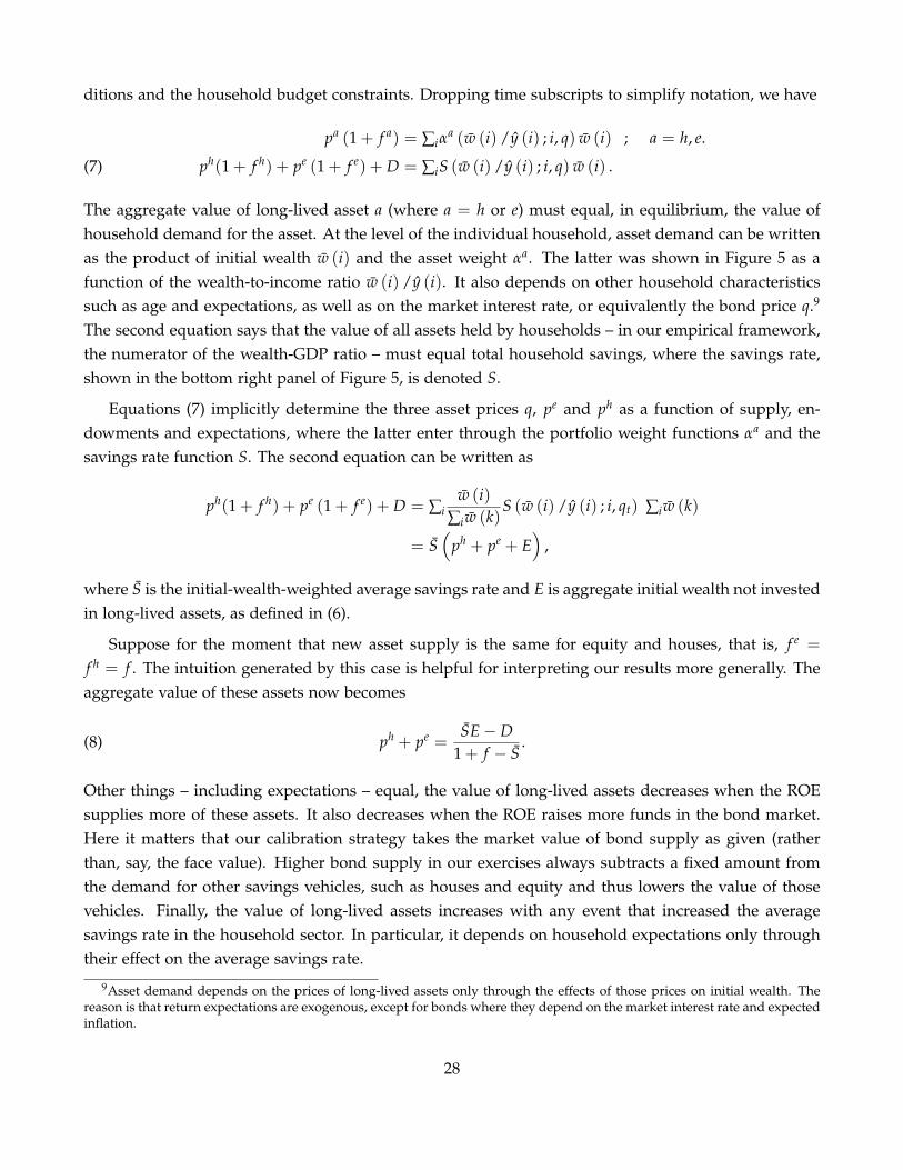
The distribution of household characteristics – in particular age and endowments – affects assetprices via the average savings rate (cf. (8), for example) as well as via average portfolio weights. Sincehouseholds have homothetic preferences, it is not obvious that features of the distribution other thanthe means matter for prices.10 Recent work on calibrated incomplete markets models has derived“approximate aggregation” results: moments of the wealth distribution beyond the mean often havelittle effect on equilibrium asset prices (see Krusell and Smith 2006 for a survey).

Approximate aggregation obtains if individual savings S (w(i)/y(i); i, q) w, viewed as a function ofinitial wealth w, are well approximated by affine functions with a common slope:

(9) S (w(i)/y(i); i, q) w ≈ a (i, q, y (i)) + b (q) w,

at least on the support of the wealth distribution. Here the key property is that b does not depend onany individual characteristics i. Assuming equal supply of equity and houses as in (8): the total valueof long lived assets is then

(10) ph + pe =a + bE− D1 + f − b

,

where a is the population-weighted average of the intercepts a. The wealth-GDP ratio thus depends onthe distribution of income only through the aggregate E.

The top panel of Figure 7 plots the ratio of savings – or terminal wealth – to the permanent com-ponent of income y as a function of the wealth-to-income ratio w/y, for the same age groups as inFigure 5. Holding age fixed, savings are well approximated by an affine function in w, if w is highrelative to y.11 Moreover, the intercept is negative and proportional to y: rich households with a higherpermanent component of income save less overall, but they save the same fraction of every additional

10In a standard general equilibrium model with identical homothetic preferences, the wealth distribution is irrelevant forprices: homotheticity leads to demand functions that are linear in wealth; if preferences are also identical, the slopes are allthe same and aggregate demand is linear in aggregate wealth.

11Comparison of Figures 5 and 7 shows that equal savings rates across individuals are sufficient, but not necessary to obtaincommon slopes b of the savings functions (9).

29

1 2 3 4 50

1

2

3

4Terminal−wealth−income ratio as a function of initial−wealth−income ratio

1 2 3 4 50

0.2

0.4

0.6

0.8

1Adjusted Cdf of initial−wealth−income−ratio by age

724735all

Figure 7: Aggregation Results

unit of wealth. While approximate aggregation obtains for rich households within an age group, thesavings function is not affine when w is low relative to y. This is true especially for the youngest agents,for whom the nonnegativity constraint on savings is most relevant. In addition, the slopes differ byage, which suggests that the wealth distribution between cohorts matters for prices.

Our framework allows to assess how much heterogeneity in wealth matters for prices by comparingthe measured wealth distribution to the model implied savings function. The bottom panel of Figure7 plots a cumulative distribution functions for the wealth-to-income ratio w/y by age. For easierinterpretation, the cdf was adjusted so that integrating the savings functions for some age group in thetop panel against the density derived from the corresponding cdf in the bottom panel yields aggregate

30

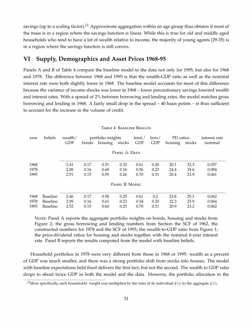
savings (up to a scaling factor).12 Approximate aggregation within an age group thus obtains if most ofthe mass is in a region where the savings function is linear. While this is true for old and middle agedhouseholds who tend to have a lot of wealth relative to income, the majority of young agents (29-35) isin a region where the savings function is still convex.

VI Supply, Demographics and Asset Prices 1968-95

Panels A and B of Table 4 compare the baseline model to the data not only for 1995, but also for 1968and 1978. The difference between 1968 and 1995 is that the wealth-GDP ratio as well as the nominalinterest rate were both slightly lower in 1968. The baseline model accounts for most of this differencebecause the variance of income shocks was lower in 1968 – lower precautionary savings lowered wealthand interest rates. With a spread of 2% between borrowing and lending rates, the model matches grossborrowing and lending in 1968. A fairly small drop in the spread – 40 basis points – is thus sufficientto account for the increase in the volume of credit.

Table 4: Baseline Results

year beliefs wealth/ portfolio weights lend./ borr/ PD ratios interest rateGDP bonds housing stocks GDP GDP housing stocks nominal

Panel A: Data

1968 2.41 0.17 0.51 0.32 0.61 0.20 20.1 32.3 0.0571978 2.08 0.16 0.68 0.16 0.56 0.23 24.4 18.6 0.0841995 2.51 0.15 0.59 0.26 0.70 0.31 20.4 23.9 0.061

Panel B: Model

1968 Baseline 2.46 0.17 0.58 0.25 0.61 0.2 23.8 25.1 0.0621978 Baseline 2.09 0.16 0.61 0.23 0.54 0.20 22.3 25.9 0.0641995 Baseline 2.52 0.15 0.60 0.25 0.70 0.31 20.9 23.2 0.062

Note: Panel A reports the aggregate portfolio weights on bonds, housing and stocks fromFigure 2; the gross borrowing and lending numbers from Section the SCF of 1962, theconstructed numbers for 1978 and the SCF of 1995; the wealth-to-GDP ratio from Figure 1;the price-dividend ratios for housing and stocks together with the nominal 6-year interestrate. Panel B reports the results computed from the model with baseline beliefs.

Household portfolios in 1978 were very different from those in 1968 or 1995: wealth as a percentof GDP was much smaller, and there was a strong portfolio shift from stocks into houses. The modelwith baseline expectations held fixed delivers the first fact, but not the second. The wealth to GDP ratiodrops to about twice GDP in both the model and the data. However, the portfolio allocation in the

12More specifically, each households’ weight was multiplied by the ratio of its individual y (i) to the aggregate y (i) .

31

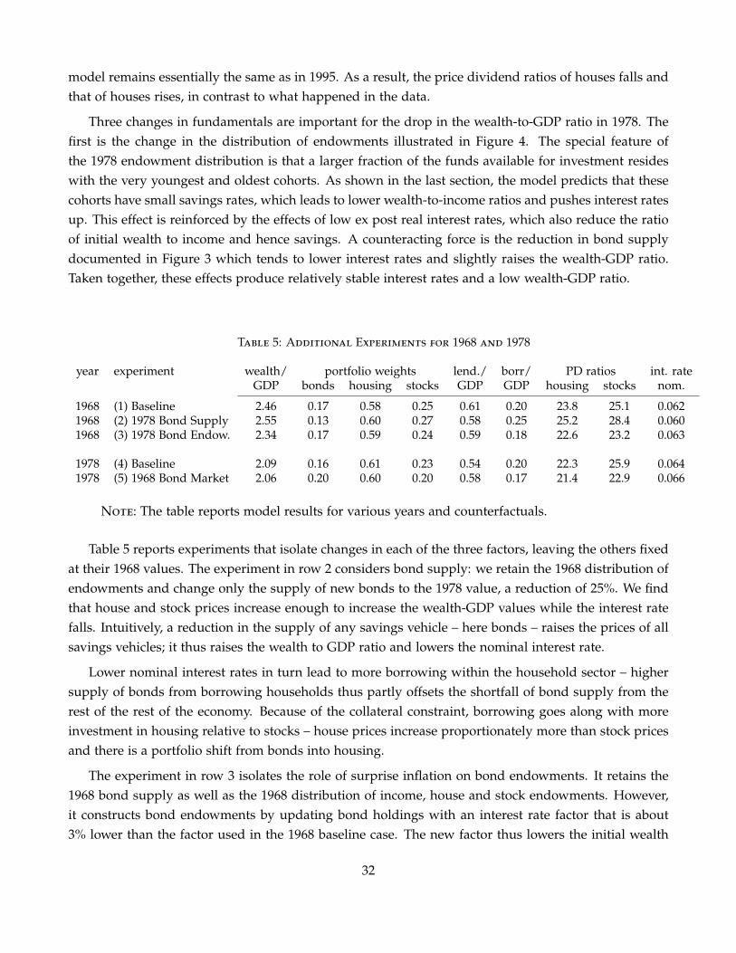
model remains essentially the same as in 1995. As a result, the price dividend ratios of houses falls andthat of houses rises, in contrast to what happened in the data.

Three changes in fundamentals are important for the drop in the wealth-to-GDP ratio in 1978. Thefirst is the change in the distribution of endowments illustrated in Figure 4. The special feature ofthe 1978 endowment distribution is that a larger fraction of the funds available for investment resideswith the very youngest and oldest cohorts. As shown in the last section, the model predicts that thesecohorts have small savings rates, which leads to lower wealth-to-income ratios and pushes interest ratesup. This effect is reinforced by the effects of low ex post real interest rates, which also reduce the ratioof initial wealth to income and hence savings. A counteracting force is the reduction in bond supplydocumented in Figure 3 which tends to lower interest rates and slightly raises the wealth-GDP ratio.Taken together, these effects produce relatively stable interest rates and a low wealth-GDP ratio.

Table 5: Additional Experiments for 1968 and 1978

year experiment wealth/ portfolio weights lend./ borr/ PD ratios int. rateGDP bonds housing stocks GDP GDP housing stocks nom.

1968 (1) Baseline 2.46 0.17 0.58 0.25 0.61 0.20 23.8 25.1 0.0621968 (2) 1978 Bond Supply 2.55 0.13 0.60 0.27 0.58 0.25 25.2 28.4 0.0601968 (3) 1978 Bond Endow. 2.34 0.17 0.59 0.24 0.59 0.18 22.6 23.2 0.063

1978 (4) Baseline 2.09 0.16 0.61 0.23 0.54 0.20 22.3 25.9 0.0641978 (5) 1968 Bond Market 2.06 0.20 0.60 0.20 0.58 0.17 21.4 22.9 0.066

Note: The table reports model results for various years and counterfactuals.

Table 5 reports experiments that isolate changes in each of the three factors, leaving the others fixedat their 1968 values. The experiment in row 2 considers bond supply: we retain the 1968 distribution ofendowments and change only the supply of new bonds to the 1978 value, a reduction of 25%. We findthat house and stock prices increase enough to increase the wealth-GDP values while the interest ratefalls. Intuitively, a reduction in the supply of any savings vehicle – here bonds – raises the prices of allsavings vehicles; it thus raises the wealth to GDP ratio and lowers the nominal interest rate.

Lower nominal interest rates in turn lead to more borrowing within the household sector – highersupply of bonds from borrowing households thus partly offsets the shortfall of bond supply from therest of the rest of the economy. Because of the collateral constraint, borrowing goes along with moreinvestment in housing relative to stocks – house prices increase proportionately more than stock pricesand there is a portfolio shift from bonds into housing.

The experiment in row 3 isolates the role of surprise inflation on bond endowments. It retains the1968 bond supply as well as the 1968 distribution of income, house and stock endowments. However,it constructs bond endowments by updating bond holdings with an interest rate factor that is about3% lower than the factor used in the 1968 baseline case. The new factor thus lowers the initial wealth

32

of lenders and increases the initial wealth of borrowers; its value is selected to make aggregate payoffson bonds as a percent of GDP as low as in 1978, where inflation significantly reduced the ex post realinterest rate.

Surprise inflation has the opposite effects from a reduction in asset supply: a lower bond endow-ment lowers initial wealth and thus reduces the demand for all savings vehicles. As a result, all assetprices fall, as does the wealth-GDP ratio. The reason is that the household sector on aggregate is a netlender so that for the majority of households (in wealth-weighted terms) the wealth-income ratio andthe savings rate go down. Of course, at the same time, borrower households experience an increase intheir wealth-income ratio, so that the distribution of wealth-income ratios becomes less dispersed. Thisexplains the drop in gross credit volumes from the experiment.

Finally, row 5 uses the 1978 distribution, including bond endowments, but fixes the bond supplyat its 1968 value. In addition, it increases the bond endowments by raising the interest rate factor byabout 3%, so that the aggregate bond endowments is also at the higher 1968 value. This is a way toisolate the effect of the income and endowment distribution from the other two factors. The main resultis a drop in the wealth-GDP ratio that is essentially the same as in the data. It is driven by the lowersavings rates of the 1978 population.

VII The Effect of Beliefs about Inflation

In this section, we consider the effects of inflation on the price-dividend ratios of real assets in the1970s. We use our model to quantify the extent to which changes in both expected inflation andinflation uncertainty contributed to higher house prices and lower stock prices. Results are reported inTable 6. Rows 1 and 2 simply repeat the statistics from Table 4 for the data and model results basedon baseline beliefs, respectively. In this section, we show how model results change as we vary beliefsabout inflation.

We begin by examining the first moment, that is, expected inflation. To measure inflation expecta-tions in the 1970s, we turn to the Michigan Survey of Consumers. Figure 8 plots population medianforecasts since 1979 together with median forecasts for different cohorts in the survey. The figure il-lustrates two key stylized facts. First, median inflation expectations across all households are highduring the late 1970s and early 1980s, and then come down. Second, households disagree systemati-cally by age. During the Great Inflation, older households expected much lower inflation than youngerhouseholds; the discrepancy vanished as inflation subsided in the 1990s.

The exercise in row 3 of Table 6, labeled “Survey Inflation Exp ”, assumes that the inflation rateexpected by an age cohort in the model is equal to the corresponding cohort median in the MichiganSurvey. The experiment generates a dramatic shift in portfolios towards housing, driven by an increasein house prices and a drop in stock prices. At the same time, the nominal interest rate rises sharply toover 10% and there is a credit boom: gross borrowing and lending increases by close to 10 percentagepoints.

33

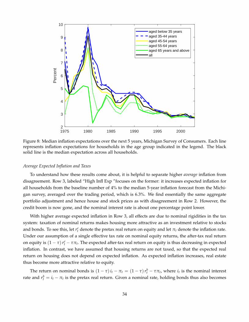
1975 1980 1985 1990 1995 20002

3

4

5

6

7

8

9

10

Per

cent

aged below 35 yearsaged 35-44 yearsaged 45-54 yearsaged 55-64 yearsaged 65 years and aboveall

Figure 8: Median inflation expectations over the next 5 years, Michigan Survey of Consumers. Each linerepresents inflation expectations for households in the age group indicated in the legend. The blacksolid line is the median expectation across all households.

Average Expected Inflation and Taxes

To understand how these results come about, it is helpful to separate higher average inflation fromdisagreement. Row 3, labeled “High Infl Exp ”focuses on the former: it increases expected inflation forall households from the baseline number of 4% to the median 5-year inflation forecast from the Michi-gan survey, averaged over the trading period, which is 6.3%. We find essentially the same aggregateportfolio adjustment and hence house and stock prices as with disagreement in Row 2. However, thecredit boom is now gone, and the nominal interest rate is about one percentage point lower.

With higher average expected inflation in Row 3, all effects are due to nominal rigidities in the taxsystem: taxation of nominal returns makes housing more attractive as an investment relative to stocksand bonds. To see this, let re

t denote the pretax real return on equity and let πt denote the inflation rate.Under our assumption of a single effective tax rate on nominal equity returns, the after-tax real returnon equity is (1− τ) re

t − τπt. The expected after-tax real return on equity is thus decreasing in expectedinflation. In contrast, we have assumed that housing returns are not taxed, so that the expected realreturn on housing does not depend on expected inflation. As expected inflation increases, real estatethus become more attractive relative to equity.

The return on nominal bonds is (1− τ) it − πt = (1− τ) rbt − τπt, where it is the nominal interest

rate and rbt = it − πt is the pretax real return. Given a nominal rate, holding bonds thus also becomes

34

less attractive as expected inflation increases, whereas mortgage borrowing becomes more attractivebecause interest is tax deductible. Put differently, the taxation of nominal interest induces an inflationpremium on top of the increase in the nominal rate warranted by the Fisher equation. This is why thenominal interest rate increases by more than the increase in expected inflation.

Disagreement about Expected Inflation

Heterogeneity in inflation expectations matters in our model because it introduces disagreementabout real returns that correlates with the propensity to take risks. Two effects explain explains thedifferences between Rows 3 and 4 of Table 6. First, old households who expect lower inflation perceiverelatively higher after-tax returns on stocks. As a result, the shift to housing discussed above is mutedfor old households who expect lower inflation than the median household. Since old households arealso more important holders of equity on aggregate, the disagreement case in Row 3 shows a higherweight on stocks as well as a higher stock price.

The second effect is that disagreement about real interest rates generates gains from trade in thecredit market. Young households – who expect high inflation – perceive a lower real interest rate thanold households who expect low inflation. The result is a credit boom: young households who arenatural borrowers believe that borrowing is a bargain and borrow from old households, who are happyto lend. Given our distribution of endowments, the relative attraction of borrowing is so large that theinterest rate has to rise substantially to choke off the credit boom. Disagreement thus moves the realrate, holding fixed average expected inflation.

Quantitatively, the changes in household portfolios in row 3 are more than enough to match theportfolio shift of the 1970s shown in row 1. However, the nominal interest rate of 10.1% is significantlyhigher than the observed rate of 8.4% and the credit boom generated by disagreement is too large. Thisreveals a basic tension between using point estimates of expected inflation and fitting moments from thecredit market. The result is perhaps not surprising. Indeed, the Great Inflation increased the volatilityof inflation, but only its mean, and it is likely that households took this into account. Moreover, thereis considerable measurement error in 1970s survey data. We now attempt to address both issues.

Inflation Uncertainty

Given the increase in many measures of inflation uncertainty during the 1970s, it is perhaps notsurprising that an asset pricing model that varies only the first moments of beliefs cannot fit the data.We now turn to the quantitative effects of inflation volatility. Unfortunately, we do not have data onperceived uncertainty directly from survey. Our strategy is thus to back out beliefs and assess whetherthis provides a parsimonious account of savings, portfolio choice and asset prices.

To provide some intuition for how inflation uncertainty works in our model, we perform a counter-factual that starts from the baseline and simply doubles inflation volatility from 3% to 6% p.a. Resultsare reported in Row 5 of Table 6, labeled “High Infl Vol ”The main difference to the baseline results isthat there is now less nominal borrowing and lending within the household sector and a higher nomi-nal interest rate. Intuitively, higher conditional volatility of inflation increases the conditional volatility

35

of real bond returns and the ex post real cost of mortgage financing. Nominal instruments thus becomeless attractive to both borrowers and lenders. The nominal interest rate increases because the householdsector as a whole is a net lender and must be compensated if it is to hold the nominal debt of the restof the economy.

Increasing inflation volatility has little effect on the overall wealth-GDP ratio. Indeed, it is a compar-ative static that affects the returns on one asset, leaving those on other assets unchanged. The overallreturn on wealth and the savings decision are not affected much and the equilibrium wealth-GDP ratiostays essentially the same. Aggregate portfolio weights also remain unchanged. On the one hand,households are required to hold the same value of bonds issued by the rest of the economy in equilib-rium, so that the portfolio weight on bonds remains unchanged if the wealth-GDP does not change. Onthe other hand, the effect of a change in the relative volatility of after tax returns on stocks and housesis quantitatively small so that the weights on stocks and houses also move little.

Table 6: The Effects of Inflation

wealth/ portfolio weights lend./ borr./ PD ratios nominalbeliefs GDP bonds housing stocks GDP GDP housing stocks int. rate

(1) — 1978 Data — 2.08 0.16 0.68 0.16 0.56 0.23 24.4 18.6 0.084(2) Baseline 2.09 0.16 0.61 0.23 0.54 0.20 22.3 25.9 0.064(3) Survey Infl Exp 2.02 0.16 0.70 0.14 0.69 0.36 24.5 15.1 0.102(4) High Infl Exp 2.01 0.17 0.71 0.12 0.52 0.18 24.9 13.3 0.091(5) High Infl Vol 2.08 0.16 0.62 0.22 0.50 0.17 22.4 25.1 0.066(6) Survey Infl Exp + Hi Infl Vol 2.02 0.16 0.70 0.14 0.56 0.23 24.5 15.1 0.108(7) Adj Infl Exp + Hi Infl Vol 2.03 0.16 0.69 0.15 0.55 0.22 24.2 16.5 0.085

Note: Rows 1 repeats the 1978 data, while row 2 contains results with baseline expectationsfrom Table 3. The other scenarios change expectations over the next six years away from thebaseline. Row 3 (“Survey Infl Exp”) sets every age cohort’s expected inflation in the modelequal to the cohort median in the Michigan Survey, averaged over 1975-80. Row 4 (“HighInfl Exp”) increases households’ expected inflation from the baseline 4% to the median 6.3%in the Michigan Survey of Consumers, averaged over 1975-1980. Row 5 (“High Infl Vol”)doubles the conditional volatility of inflation. Row 6 (“Survey Infl Exp + Hi Infl Vol”) usesexpected cohort inflation rates (as in row 3) and increase the volatility of inflation by a factorof 3.5 Row 7 (“Adj Infl Exp + Hi Infl Vol”) shifts expected inflation down by 1pp per yearfor all cohorts.

We now ask whether there is a parsimonious parametrization of beliefs that avoids the tensionbetween effects on long-lived asset markets and the credit market. We proceed in two steps. First, weask what the perceived volatility of inflation would have to be so the model matches the volume ofcredit. Row 6 of Table 5 starts from heterogeneous expectations (row 3), but increases the volatility ofinflation by a factor of 3.5. As expected from the comparison of rows 1 and 5 above, the only effectis that credit drops to match the data, and there is a small increase in the interest rate. We conclude

36

that there are no important interaction between disagreement and perceived volatility – the two beliefparameters impact different moments of the data.

The final experiment in Row 7 shifts down the schedule of expected inflation by 1pp per year forall cohort. We thus continue to match cross-cohort differences in expected inflation and only adjust themean. The adjustment shift is within two standard errors of the point estimates for the cohort medians,and hence still represents a plausible scenario, given the uncertainty about survey expectations duringthis period. The result is that we can now jointly match wealth-GDP, portfolio weights, the volumeof credit and interest rates. We conclude that introducing inflation expectations that are broadly inline with survey evidence can account for the strong portfolio shift across assets. Together with demo-graphics – which according to the last row in Table 5 is responsible for joint downward movement inlong-lived wealth positions – we arrive at an account for the 1970s driven primarily by the two uniqueevents of the decade.

37

References

Abel, Andrew B., “The Effects of a Baby Boom on Stock Price and Capital Accumulation in the Presence of SocialSecurity.,” Econometrica, 2003, 71 (2), 551–578.

Ameriks, John, Joseph Briggs, Andrew Caplin, Matthew D. Shapiro, and Chris Tonetti, “Long-Term-CareUtility and Late-in-Life Saving,” Forthcoming Journal of Political Economy, 2020.

Campbell, John Y. and Joao F. Cocco, “Household Risk Management and Optimal Mortgage Choice.,” 2003.

Chien, YiLi, Harold Cole, and Hanno Lustig, “Is the Volatility of the Market Price of Risk Due to IntermittentPortfolio Rebalancing?,” American Economic Review, 2012, 102 (6), 2859–2896.

, , and , “Implications of heterogeneity in preferences, beliefs and asset trading technologies in an endow-ment economy,” Review of Economic Dynamics, 2016, 20, 215–239.

Cocco, Joao F., “Portfolio Choice in the Presence of Housing,” Review of Financial Studies, 2005, 18, 535–567.

Cogley, Timothy and Thomas J. Sargent, “Evolving Post-World War II U.S. Inflation Dynamics,” NBER Macroe-conomics Annual, 2001, 16, 331–373.

Constantinides, George M. and Darrell Duffie, “Asset Pricing with Heterogeneous Consumers.,” Journal ofPolitical Economy, 1996, 104 (2), 219–40.

, John B. Donaldson, and Rajnish Mehra, “Junior Can’t Borrow: A New Perspective on the Equity PremiumPuzzle,” Quarterly Journal of Economics, 2002, 117, 269–296.

DeNardi, Mariacristina, Eric French, and John B. Jones, “Why do the Eldery Save? The Role of MedicalExpenses,” Journal of Political Economy, 2010, 118 (1), 39–75.

, , and John Jones, “Savings After Retirement: A Survey,” The Annual Review of Economics, 2016, 8, 177–204.

Doepke, Matthias and Martin Schneider, “Inflation and the Redistribution of Nominal Wealth,” Journal of Polit-ical Economy, 2006, 114 (6), 1069–1097.

Eggertsson, Gauti B., Neil R. Mehrotra, and Jacob A. Robbins, “A Model of Secular Stagnation: Theory andQuantitative Evaluation,” American Economic Journal: Macroeconomics, 2019, 11 (1), 1–48.

Favilukis, Jack, Syndey C. Ludvigson, and Stijn van Nieuwerburgh, “The Macroeconomic Effects of HousingWealth, Housing Finance, and Limited Risk Sharing in General Equilibrium.,” Journal of Political Economy, 2017,125 (1), 140–223.

Feldstein, Martin, “Inflation and the Stock Market.,” American Economic Review, 1980, 70 (5), 839–847.

Fernandez-Villaverde, Jesus and Dirk Krueger, “Consumption and Saving over the Life Cycle: How Importantare Consumer Durables?,” Macroeconomic Dynamics, 2011, 15 (5), 725–770.

Flavin, Marjorie and Takashi Yamashita, “Owner-Occupied Housing and the Composition of the HouseholdPortfolio.,” American Economic Review, 2002, pp. 345–62.

Gagnon, Etienne, Benjamin K. Johannsen, and David Lopez-Salido, “Understanding the New Normal: TheRole of Demographics,” Finance and Economics Discussion Series of the Board of Governors, 2016, 2016-080.

Geanakoplos, John, Michael Magill, and Martine Quinzii, “Demography and the Long-run Predictability ofthe Stock Market.,” Brookings Papers on Economic Activity, 2004, 1, 241–307.

Gomes, Francisco and Alex Michaelides, “Optimal Life-Cycle Asset Allocation: Understanding the EmpiricalEvidence,” Journal of Finance, 2005, 60 (2), 869–904.

38

Gourinchas, Pierre-Olivier and Jonathan Parker, “Consumption over the Life Cycle,” Econometrica, 2002, 70,47–89.

Hansen, Lars Peter and Kenneth J. Singleton, “Generalized Instrumental Variables Estimation of NonlinearRational Expectations Models,” Econometrica, 1982, 50 (5), 1269–1286.

Heathcote, Jonathan, Kjetil Storesletten, and Giovanni L. Violante, “The Macroeconomic Implications of RisingWage Inequality in the United States,” Journal of Political Economy, 2010, 118 (4), 681–722.

Heaton, John and Deborah J. Lucas, “Evaluating the Effects of Incomplete Markets on Risk Sharing and AssetPricing,” Journal of Political Economy, 1996, 104, 443–487.

and , “Portfolio Choice and Asset Prices: The Importance of Entrepreneurial Risk,” Journal of Finance, 2000,55, 1163–1198.

Ilut, Cosmin and Martin Schneider, “Ambiguous Business Cycles,” American Economic Review, 2014, 104, 2368–2399.

Jagannathan, Ravi and Narayana Kocherlakota, “Why Should Older People Invest Less in Stocks Than YoungerPeople?,” Quarterly Review of the Federal Reserve Bank of Minneapolis, 1996, 20 (3), 11–23.

Justiniano, Alejandro, Giorgio E. Primiceri, and Andrea Tambalotti, “Credit Supply and the Housing Boom,”Journal of Political Economy, 2019, 127 (3), 1317–1350.

Krueger, Dirk and Felix Kubler, “Computing equilibrium in OLG models with stochastic production,” Journalof Economic Dynamics and Control, 2004, 58 (7), 1411–1436.

Krusell, Per and Anthony Smith, “Income and Wealth Heterogeneity in the Macroeconomy,” Journal of PoliticalEconomy, 1998, 106 (5), 867–896.

Landvoigt, Tim, Monika Piazzesi, and Martin Schneider, “The Housing Market(s) of San Diego,” AmericanEconomic Review, 2015, 105 (4), 1371–1407.

Malmendier, Ulrike and Stefan Nagel, “Learning from Inflation Experiences,” Quarterly Journal of Economics,2016, 131 (1), 53–87.

Mankiw, Gregory N. and David Weil, “The Baby Boom, the Baby Bust and the Housing Market,” Regional Scienceand Urban Economics, 1989, 19, 235–258.

Ortalo-Magne, Francois and Sven Rady, “Housing Market Dynamics: On the Contribution of Income Shocksand Credit Constraints.,” Review of Economic Studies, 2006, 73 (2), 459–485.

Piazzesi, Monika and Martin Schneider, “Housing and Macroeconomics,” Handbook of Macroeconomics, 2016, 2,1547–1640.

, , and Selale Tuzel, “Housing, Consumption and Asset Pricing,” Journal of Financial Economics, 2007, 83,531–569.

Poterba, James, “House Price Dynamics: The Role of Tax Policy and Demographics.,” Brookings Papers on EconomicActivity, 1991, 2, 143–203.

Sialm, Clemens, “Tax Changes and Asset Pricing,” American Economic Review, 2009, 99 (4), 1356–1383.

Storesletten, Kjetil, Chris I. Telmer, and Amir Yaron, “Asset pricing with idiosyncratic risk and overlappinggenerations,” Review of Economic Dynamics, 2007, 10 (4), 519–548.

Summers, Lawrence H., “Inflation, the Stock Market, and Owner-Occupied Housing,” American Economic Review,1981, 71, 429–434.

39

Yao, Rui and Harold Zhang, “Optimal Portfolio Choice with Risky Housing and Borrowing Constraints.,” Reviewof Financial Studies, 2005, 18, 197–239.

Zeldes, Stephen P., “Optimal Consumption with Stochastic Income: Deviations from Certainty Equivalence,”Quarterly Journal of Economics, 1989, 104, 275–298.

40

Appendix

A Assets and Income

This appendix describes how we map observed asset classes into the three assets present in the model,and how we measure aggregate and household level asset holdings, as well as non-asset income.

A. Data and Definitions

We map the three assets in the model to three broad asset classes in US aggregate and household statis-tics. Our main data sources are the Financial Accounts of the United States (FAUS) for aggregates andthe Survey of Consumer Finances (SCF) for individual positions. To make these data sets comparable,we must ensure that aggregates match. As shown by Antoniewicz (2004), the match is good for mostasset classes in both 1989 and 1995, after a few adjustments. However, our own computations show thatthe match for nominal assets is bad for the 1962 SCF. For some classes of assets, especially short-termdeposits, the SCF aggregates are only about 50% of the FAUS aggregates. Apparent underreporting ofshort-term nominal assets is also present in later SCFs, but is less severe. To achieve a comparable timeseries of positions, we assume throughout that the FAUS aggregates are correct and that individualpositions in the SCF suffer from proportional measurement error. We then multiply each individualposition by the ratio of the FAUS aggregate and the SCF aggregate for the same asset class.

Asset classes

We identify equity with shares in corporations held and controlled by households, including bothpublicly traded and closely held shares, and both foreign and domestic equity. We also include sharesheld indirectly through investment intermediaries if the household can be assumed to control theasset allocation (into our broad asset classes). We take this to be true for mutual funds and definedcontribution (DC) pensions plans. For these intermediaries, while the fund manager determines theprecise composition of the portfolio, the household typically makes the decision about equity versusbonds by selecting the type of fund.

We thus consolidate mutual funds and DC pension funds. For example, when households owna mutual fund, an estimate of the part of the fund invested in stocks is added to stock holdings. Incontrast, we do not include equity held in defined benefit (DB) pension plans, since the portfolios ofthese plans are not controlled by households themselves. Instead, DB plans are treated as a tax-transfersystem sponsored by the rest of the economy (in practice, the corporate sector or the government). Wealso do not include noncorporate business, which is treated partly as real estate and partly as laborincome, as described below.

We construct an annual series for the aggregate value of household sector equity holdings. Ourstarting point is the published series in the FAUS. We cannot use that series directly, since it contains(i) the market value of the equity component of foreign direct investment (that is, equity positions byforeigners in excess of 10% of shares in a US corporation) and (ii) the market value of equity held by DBpension funds. We estimate the equity component of FDI using data on the International Investment

41

Position from the Bureau of Economic Analysis. Shares held by defined benefit pension funds areavailable from the FAUS. Our series is obtained by subtracting (i) and (ii) from the FAUS series onhousehold equity holdings.

We derive estimates of net new equity purchased by households using a similar correction of FAUSnumbers. Finally, our concept of dividends equals dividends received by households from the NationalIncome and Product Accounts (NIPA) less dividends on their holdings in DB pension plans. We usethe numbers on value, dividends and new issues to calculate price dividend ratios and holding returnson equity. The properties of the return series are discussed in Appendix B below. For household-levelpositions, we use the Survey of Consumer Finances, which also contains direct holdings of publicly-traded and closely-held shares, as well as an estimate of equity held indirectly through investmentintermediaries.

Our concept of residential real estate contains owner-occupied housing, directly held residential in-vestment real estate, as well as residential real estate recorded in the FAUS/NIPA as held indirectly byhouseholds through noncorporate businesses. This concept contains almost all residential real estateholdings, since very few residential properties are owned by corporations. To construct holdings oftenant-occupied residential real-estate at the individual level, we start from the SCF numbers and thenadd a proportional share of the household’s noncorporate business position. This share is selected sothat our aggregate of tenant-occupied real estate over all households matches the corresponding valuefrom the FAUS. We take housing dividends to be housing consumption net of maintenance and prop-erty tax from NIPA. For net purchases of new houses, we use aggregate residential investment fromNIPA. As with equity, the annual series for holdings, dividends and new issues give rise to a returnseries, discussed below.

Household bond holdings are set equal to the net nominal position, that is, the market value ofall nominal assets minus the market value of nominal liabilities. Nominal assets again include indi-rect holdings through investment intermediaries. To calculate market value, we use the market valueadjustment factors for nominal positions in the U.S. from Doepke and Schneider (2006). In line withour treatment of tenant-occupied real estate, we assign residential mortgages issued by noncorporatebusinesses directly to households. At the individual level, we assign a household mortgages in propor-tion to his noncorporate business position, again with a share selected to match the aggregate value ofresidential mortgages from the FAUS.

Non-Asset Income

Our concept of non-asset income comprises all income that is available for consumption or invest-ment, but not received from payoffs of one of our three assets. We start by constructing an aggregatemeasure of such income from NIPA. Of the various components of worker compensation, we includeonly wages and salaries, as well as employer contributions to DC pension plans. We do not includeemployer contributions to DB pension plans or health insurance, since these funds are not availablefor consumption or investment. However, we do include benefits disbursed from DB plans and healthplans. Also included are transfers from the government. Finally, we subtract personal income tax on

42

non-asset income.

Non-asset income also includes dividends from noncorporate business except those attributable toresidential real estate. To construct the latter concept of noncorporate dividends, we use the aggregateprice-dividend ratio of housing to estimate the housing dividend provided by an individual’s privatebusiness. Our approach essentially splits up the noncorporate sector into a real estate component thatis very capital intensive and relies heavily on debt finance, and a rest that is much more labor intensive.Indeed, the capital stock of the noncorporate nonfinancial sector in 1995 was $3.6trn, of which $2.4trnwas residential real estate.

Given the aggregate series of income, we apply the same conventions to individual income in theSCF to the extent possible. A problem is that the SCF does not report employer contributions to DCplans and only reports pretax income for all items. To address this issue, we apply a proportional taxrate to pretax non-asset income reported in the SCF, where the tax rate is chosen such that aggregatenon-asset income is equal to its counterpart from NIPA. The outcome is an income distribution thatmatches with NIPA at the aggregate level.

B. Measuring the Distribution of Endowments

Consumers in our model are endowed with both assets and non-asset income. To capture decisionsmade by the cross-section of households, we thus have to initialize the model for every period t with ajoint distribution of asset endowment and income. We derive this distribution from asset holdings andincome observed in the previous period t− 1. Limits on data availability imply that we have to resortto different approaches for the different years. For 1995, the data situation is best, since we can use theSCF in the 4th year of period t together with the SCF from the 4th year of period t− 1. We describeour strategy first for this case. We then explain how it is modified for earlier years where less data areavailable.

Approximating the distribution of households

In principle, one could use all the households in SCF and update them individually. This wouldlead to a large number of agents and consequently a large number of portfolio problems would haveto be solved. We simplify by approximating the distribution of endowments and income with a smallnumber of household types. First, we sort households into the same nine age groups described at thebeginning of this section. Within each age group, we then select 6 subclasses of SCF households. Westart by extracting the top 10% of households by net worth. Among the bottom 90% net worth, wedivide by homeowner and renter. We then divide homeowners further into “borrowers” and “lenders.”Here a household is a borrower if his net nominal position – nominal asset minus nominal liabilities –is negative. We further subdivide each homeowner category into high/low wealth-to-income ratios.

The above procedure splits up households into 9 × 6 = 54 different cells. We assume that allhouseholds that fall into the same cell are identical and compute asset positions at the cell level. TheSCF survey weights determine the cell population. Naturally, the procedure loses some features ofthe true distribution due to aggregation. However, it ensures that key properties of the distribution

43

that we are interested in are retained. In particular, because very few among the top 10% are netnominal borrowers, gross borrowing and lending are very close in the true and the approximatingdistributions. In addition, the approximating distributions retains asset positions conditional on ageas well as conditional on wealth when net worth is split as top 10% and the rest, our key measures ofconcentration described.

Asset endowments for a transiting individual household

Consider the transition of an individual household’s asset position from period t − 1 into periodt. We have treated both stocks and houses as long-lived trees and we normalize the number of treescarried into the period by consumers to one. We can thus measure the household’s endowment ofa long-lived asset from its share in total market capitalization of the asset in period t − 1. The SCFdoes not contain consumption data. Using the language introduced in the discussion of the budgetconstraint (4), we can thus measure either initial or terminal wealth in a given period, but not both.We assume that terminal wealth can be directly taken from the survey. The initial supply of assets isnormalized to one, so that the initial holdings of housing θh

t and stocks θet are the agent’s market shares

in period t− 1. For each long-lived asset a = h, e, suppose that wat−1 (i) is the market value of investor

i’s position in t− 1 in asset a. Now we can measure household i’s initial holdings as

θat (i) = θa

t−1 (i) =wa

t−1 (i)∑iwa

t−1 (i)=

pat−1 θa

t−1 (i)pa

t−1∑iθat−1 (i)

= market share of household i in period t− 1.

Updating Nominal Positions

For the nominal assets, the above approach does not work since these assets are short-term in ourmodel. Instead, we determine the market value of nominal positions in period t− 1 and update it toperiod t by multiplying it with a nominal interest rate factor. In particular, suppose that wb

t−1 (i) is themarket value of investor i’s net nominal positions in t− 1 and that

θbt−1 (i) =

wbt−1 (i)

∑iwbt−1 (i)

= market share of household i in period t− 1.

We define the initial holdings of bonds for household i as

bt (i) = (1 + it−1)wb

t−1 (i)GDPt

= (1 + it−1)wb

t−1 (i)

∑iwbt−1 (i)

∑iwbt−1 (i)

GDPt−1

GDPt−1

GDPt.

As an interest factor for a positive (lending) position, we use an average of 6-year bond rates betweenthe 4th year of period t and the 4th year of period t− 1. We add a spread for the borrowing rate. Thespread is 2% for 1995 and 2.75% for 1968 and 1978, for reasons described in the calibration section IV.

44

Forecasting Income

The final step in our construction of the joint income and endowment distribution is to specify themarginal distribution of non-asset income. Here we make use of the fact that income is observed inperiod t − 1 in the SCF. We then assume that the transition between t − 1 and t is determined by astochastic process for non-asset income. We employ the same process that agents in the model use toforecast their non-asset income, described in the next subsection. If the assumption were true, and ifthere were a large number of identical individuals in every cell, then our discretization implies thathouseholds in a cell should split up into nine different cells in the following period, with fractions pro-vided by the probabilities of the income process. This is what we assume. As a result, the distributionof agents in period t is approximated by 9 × 6 × 9 = 486 different cells. For each cell, we know theendowment of assets as well as income, and we have a set of population weights that sums to the totalpopulation.

Non-transiting households

The previous discussion has covered only households who transit from period t into period t + 1.We also need to take into account the creation and destruction of households between t− 1 and t. Inyears where successive SCFs are available, we calculate “birthrates” and “deathrates” for householdsdirectly by comparing these surveys. We assume that exiting households receive no labor income,but sell their assets and consume the proceeds, while entering households start with zero assets andthe average labor income of their cohort. This is a simplified view that does not do justice to themany different reasons why households form and dissolve, and how wealth is passed along amonghouseholds. However, we view it as a useful benchmark.

Time periods without two successive SCFs

For periods before 1980, the above strategy cannot be executed as is, because we do not have twoconsecutive SCFs. For the period 1965-70, the 1962 SCF is used to determine the initial endowmentand income distribution. The only difficulty here is the adjustment of exiting and entering households.We use data from the Census Bureau on the evolution of household populations to gauge the size ofexiters and entrants. The average labor income of the entering cohort is then estimated by multiplyingper capita income of the young in the 1962 SCF by the growth rate of aggregate per capita labor income.

For the period 1975-80, we do not have SCF information for period t − 1. As for the 1960s, theupdating of population weights is performed using Census data. To estimate the cross sectional distri-bution of endowments and income, we start from the 1962 distribution and its division of householdsinto cells and modify cell holdings to obtain a new distribution. In particular, we calculate the uniquedistribution such that, for stocks, real estate, nominal assets, nominal debt and income, (i) aggregatesmatch the aggregates from the FAUS for the period 1969-74, (ii) the ratio of holdings between individ-ual members of any two cells is the same as in the 1962 SCF and (iii) the relative size of a cell withinits age cohort is the same as in the 1962 SCF.

Condition (i) and (ii) imply that per capita holdings or income within a cohort changes in order

45

to account for differences in demographics while simultaneously matching aggregates. Conditions (ii)and (iii) imply that the cross section conditional on age is the same in the two years. The reason forusing the 1962 distribution as the starting point rather than, say the 1989 distribution, is that the early1970s aggregates – especially gross nominal assets – appear more similar to 1962 than to aggregatesfrom the 1980s. Once we have a distribution of positions at the cell level for 1969-74, we proceed asabove to generate an updated distribution for 1975-80.

C. Asset Supply

The endowment of the ROE sector consists of new equity issued during the trading period. The factorf e states this endowment relative to total market capitalization in the model. We thus use net newcorporate equity divided by total household holdings of corporate equity. We obtain the correspondingmeasure for housing by dividing residential investment by the value of residential real estate. Thecalibration of the model uses six-year aggregates. The initial nominal position of the ROE is taken tobe minus the aggregate (updated) net nominal position of the household sector. Finally, the new netnominal position of the ROE sector in period t – in other words, the “supply of bonds” to the householdsector – is taken to be minus the aggregate net nominal positions from the FAUS for period t.

B Baseline Expectations

This appendix describes agents’ expectations about returns and income in the future under the baselinescenario.

Non-Asset Income

We specify a stochastic process to describe consumer expectations about after-tax income. Thefunctional form for this process is motivated by existing specifications for labor income that employa deterministic trend to capture age-specific changes in income, as well as permanent and transitorycomponents. In particular, following Zeldes (1989) and Gourinchas and Parker (2002), we assume thatindividual income Yi is

Yit = Gt AtPi

t Uit

which has a common component Gt, an age profile At, a permanent idiosyncratic component Pit and a

transitory idiosyncratic component Uit.

The growth rate of the common component Gt is equal to the growth rate of aggregates, suchas GDP and aggregate income, in the economy. It is common to specify the transitory idiosyncraticcomponent as lognormally distributed

ln Uit = N

(−1

2σ2

u , σ2u

),

so that Uit is i.i.d with mean one. The permanent component Pi

t follows a random walk with mean one.The permanent component solves

ln Pit = ln Pi

t−1 + εit −

12

σ2ε ,

46

where εit are normal shocks with zero mean and standard deviation σ

(εi

t)

. In our numerical procedures,we discretize the state process using Gauss–Hermite quadrature with three states.

We estimate the age profile Gt as average income in each age-cohort from the SCF:

1#a ∑

i∈aYi

t = AtGt1#a ∑

i∈aPi

t ,

with plim 1#a ∑i∈a Pi

t = 1. Table B.1 reports the profile relative to the income of the youngest cohort.

Table B.1: Income Age profile

29 35 41 47 53 59 65 71 77 88+2.04 2.51 3.17 3.80 4.56 3.81 3.00 1.93 1.42 1.17

Note: Income age profiles estimated from the SCF. The numbers represent the averagecohort income relative to the average income of the youngest cohort (≤ 23 years).

We obtain an estimate of the variance of permanent shocks by computing the cross-sectional vari-ance of labor income for each cohort before retirement (<65 years) and then regressing it on a constantand cohort age. The intercept of this regression line is .78, while the annualized slope coefficient is.014.13 We thus set σ2

ε = 1.4% and time-aggregate this variance for our six-year periods. This number isin line with more sophisticated estimations of labor income processes, which tend to produce estimatesbetween 1% and 2% per year.

Typical estimates of the variance of temporary shocks σ2u are 2-10 times larger than those of the vari-

ance of permanent shocks. Moreover, several studies have shown that the variance of temporary shocksto log wages has increased since the 1970s. For example, Heathcote, Storesletten and Violante (2010)show that the variance of log wages increased from about .05 in the 1970s to .07 in 1995. To capture thisincrease in temporary income risk, we adopt their numbers, thus assuming that the variance of hours isconstant. We set σ2

u = .05 for the years 1968 and 1978 and σ2u = .07 for 1995.14 In all years, agents in the

model assume that this variance is fixed forever. Finally, we determine the variance of the first draw ofpermanent income from the intercept of our regression line. For the earlier years, we scale down thisinitial variance by the relative change in the permanent component of income for the youngest agentsin Heathcote et al. This is a simple way to accommodate changes in income due to education over time.Sensitivity checks have shown that the initial draw of permanent income does not matter much for theresults, since it does not directly affect the portfolio problem.

13Of course, this simple approach uses only the cross-section and thus potentially confounds age and time or cohort effects.However, when we rerun the regression with SCF wages, using the similar sample selection criteria as Heathcote, Storeslettenand Violante (2010), our results are close to what these authors find for 1995 from an analysis with panel data on wages.

14The fixed effects only matter for the updating of the income distribution, as explained in the previous section. The model’sresults are not sensitive to the magnitude of these effects. For example, the results based on our model are unchanged whenwe use the estimates provided by Heathcote, Storesletten and Violante (2010).

47

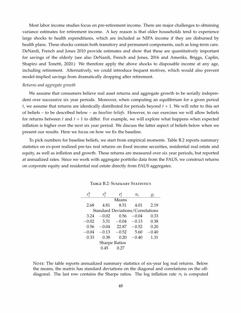
Most labor income studies focus on pre-retirement income. There are major challenges to obtainingvariance estimates for retirement income. A key reason is that older households tend to experiencelarge shocks to health expenditures, which are included as NIPA income if they are disbursed byhealth plans. These shocks contain both transitory and permanent components, such as long-term care.DeNardi, French and Jones 2010 provide estimates and show that these are quantitatively importantfor savings of the elderly (see also DeNardi, French and Jones, 2016 and Ameriks, Briggs, Caplin,Shapiro and Tonetti, 2020.) We therefore apply the above shocks to disposable income at any age,including retirement. Alternatively, we could introduce bequest motives, which would also preventmodel-implied savings from dramatically dropping after retirement.

Returns and aggregate growth

We assume that consumers believe real asset returns and aggregate growth to be serially indepen-dent over successive six year periods. Moreover, when computing an equilibrium for a given periodt, we assume that returns are identically distributed for periods beyond t + 1. We will refer to this setof beliefs – to be described below – as baseline beliefs. However, in our exercises we will allow beliefsfor returns between t and t + 1 to differ. For example, we will explore what happens when expectedinflation is higher over the next six year period. We discuss the latter aspect of beliefs below when wepresent our results. Here we focus on how we fix the baseline.

To pick numbers for baseline beliefs, we start from empirical moments. Table B.2 reports summarystatistics on ex-post realized pre-tax real returns on fixed income securities, residential real estate andequity, as well as inflation and growth. These returns are measured over six year periods, but reportedat annualized rates. Since we work with aggregate portfolio data from the FAUS, we construct returnson corporate equity and residential real estate directly from FAUS aggregates.

Table B.2: Summary Statistics

rbt rh

t ret πt gt

Means2.68 4.81 8.51 4.01 2.19

Standard Deviations/Correlations3.24 −0.02 0.56 −0.04 0.33−0.02 3.31 −0.04 −0.13 0.38

0.56 −0.04 22.87 −0.52 0.20−0.04 −0.13 −0.52 5.60 −0.40

0.33 0.38 0.20 −0.40 1.31Sharpe Ratios0.45 0.27

Note: The table reports annualized summary statistics of six-year log real returns. Belowthe means, the matrix has standard deviations on the diagonal and correlations on the off-diagonal. The last row contains the Sharpe ratios. The log inflation rate πt is computed

48

using the CPI, while gt is the log growth rate of GDP multiplied by the factor 2.2/3.3 tomatch the mean growth rate of consumption.

Baseline beliefs assume that the payoff on bonds 1/πt+1 is based on a (net) inflation rate πt+1 − 1with a mean of 4% per year, and that the volatility of πt+1 is the same as the unconditional volatilityof real bond returns, about 1.3% per year. To obtain capital gains from period t to t + 1, we take thevalue of total outstandings from the FAUS in t + 1, and subtract the value of net new issues (or, in thecase of real estate, new construction.) To obtain dividends on equity in period t, we use aggregate netdividends. To obtain dividends on real estate, we take total residential housing sector output from theNIPA, and subtract materials used by the housing sector. For bond returns, we use a six year nominalinterest rate derived by extrapolation from the term structure in CRSP, and subtract realized inflation,measured by the CPI. Here growth is real GDP growth.

The properties of the equity and bond returns are relatively standard. The return on bonds has alow mean of 2.7% and a low standard deviation of 3.2%. The return on stocks has a high mean of 8.5%and a standard deviation of 23%. What is less familiar is the aggregate return on residential real estate:it has a mean and standard deviation in between the other two assets. It is apparent that the Sharperatio of aggregate housing is much higher than that on stocks.

In principle, we could use the numbers from Table B.2 directly for our benchmark beliefs. However,this would not capture the tradeoff faced by the typical individual household. Indeed, the housingreturns in Table B.2 are for the aggregate housing stock, while real estate is typically a non-diversifiedinvestment. It is implausible to assume that investors were able to pick a portfolio of real estate withreturn characteristics as in Table B.2 at any time over our sample period. Instead, the typical investorpicks real estate by selecting a few properties local markets.

Existing evidence suggests that the volatility of house returns at the metro area, and even at theneighborhood or property level are significantly higher than returns at the national aggregate. Forexample, Caplin et al. (1997) argue that 1/4 of the overall volatility is aggregate, 1/4 is city-component,and 1/2 is idiosyncratic. Tables 1A and 1B in Flavin and Yamashita (2002) together with Appendix C inPiazzesi, Schneider and Tuzel (2007) confirm this decomposition of housing returns. As a simple wayto capture this higher property-level volatility, we add idiosyncratic shocks to the variance of housingreturns that have volatility equal to 3.5 times aggregate volatility. The resulting overall volatility ofthe return on an individual property is then 11%, consistent with the estimates in Landvoigt, Piazzesiand Schneider (2015). Finally, we assume that expected future real rents are constant. This ignores thevolatility of real rent growth, which is small, at around 2% per year.

Taxes on investment

Investors care about after-tax real returns. In particular, taxes affect the relative attractiveness ofequity and real estate. On the one hand, dividends on owner-occupied housing are directly consumedand hence not taxed, while dividends on stocks are subject to income tax. On the other hand, capitalgains on housing are more easily sheltered from taxes than capital gains on stocks. This is because

49

many consumers simply live in their house for a long period of time and never realize the capitalgains. Capital gains tax matters especially in inflationary times, because the nominal gain is taxed: theeffective real after tax return on an asset subject to capital gains tax is therefore lower when inflationoccurs.

To measure the effect of capital gains taxes, one would ideally like to explicitly distinguish realizedand unrealized capital gains. However, this would involve introducing state variables to keep trackof past individual asset purchase decisions. To keep the problem manageable, we adopt a simplerapproach: we adjust our benchmark returns to capture the effects described above. For our baselineset of results, we assume proportional taxes, and we set both the capital gains tax rate and the incometax rate to 20%. We define after tax real stock returns by subtracting 20% from realized net real stockreturns and then further subtracting 20% times the realized rate of inflation to capture the fact thatnominal capital gains are taxed. In contrast, we assume that returns on real estate are not taxed.

50