Measurement 44 (2011) 802–814

Contents lists available at ScienceDirect

Measurement

journal homepage: www.elsevier .com/ locate /measurement

Impact of sensor characteristics on source characterizationfor dispersion modeling

Luna M. Rodriguez a,b,c, Sue Ellen Haupt a,b,c,⇑, George S. Young b

a P.O. Box 30, Applied Research Laboratory, The Pennsylvania State University, State College, PA 16804-0030, United Statesb 503 Walker Building, Meteorology Department, The Pennsylvania State University, University Park, PA 16802, United Statesc P.O. Box 3000, The National Center for Atmospheric Research/Research Applications Laboratory, Boulder, CO 80307-3000, United States

a r t i c l e i n f o

Article history:Received 9 September 2010Received in revised form 7 January 2011Accepted 20 January 2011Available online 2 February 2011

Keywords:Sensor thresholdsSensor saturationDispersion monitoringDispersion modelingSource characterizationSource term estimationGenetic algorithm

0263-2241/$ - see front matter � 2011 Elsevier Ltddoi:10.1016/j.measurement.2011.01.014

⇑ Corresponding author. Tel.: +1 303 497 2763; faE-mail addresses: lmr257@psu.edu (L.M. Ro

asme.org (S. Ellen Haupt), young@meteo.psu.edu (G

a b s t r a c t

An accidental or intentional release of hazardous chemical, biological, radiological, ornuclear material into the atmosphere obligates responsible agencies to model its transportand dispersion in order to mitigate the effects. This modeling requires input parametersthat may not be known and must therefore be estimated from sensor measurements ofthe resulting concentration field. The genetic algorithm (GA) method used here has beensuccessful at back-calculating not only these source characteristics but also the meteoro-logical parameters necessary to predict the contaminants subsequent transport and disper-sion. This study assesses the impact of sensor thresholds, i.e. the sensor minimumdetection limit and saturation level, on the ability of the algorithm to back-calculate mod-eling variables. The sensitivity of the back-calculation to these sensor constraints is ana-lyzed in the context of an identical twin approach, where the data is simulated using thesame Gaussian Puff model that is used in the back-calculation algorithm in order to analyzesensitivity in a controlled environment. The solution is optimized by the GA and furthertuned with the Nelder–Mead downhill simplex algorithm. For this back-calculation to besuccessful, it is important that the sensor capture the maximum concentrations.

� 2011 Elsevier Ltd. All rights reserved.

1. Introduction of an airborne contaminant from the sensor field measure-

When a toxic agent is released into the atmosphere,government agencies are tasked with tracking and fore-casting its transport and dispersion [1–4]. These scenariosinclude both accidental and intentional release of anychemical, biological, radiological, or nuclear (CBRN) con-taminant that can be a threat to human and ecologicalhealth. Although tracking the contaminant can be accom-plished with arrays of sensors, forecasting the transportand dispersion requires input variables describing thesource of the release and the meteorological conditions.Sometimes, however, there is inadequate a priori sourceor meteorological information to perform those predic-tions and it becomes necessary to characterize the source

. All rights reserved.

x: +1 303 497 8386.driguez), haupts2@.S. Young).

ments of the resulting concentration field. Such sourceterm estimation involves back-calculating the source loca-tion and emission rate history. There has been extensivework on methods for back-calculating source characteris-tics. For example, Thompson et al. [5] use a random searchalgorithm with simulated annealing and Rao [6] reviewsmethods that include adjoint and tangent linear models,Kalman filters, and variational data assimilation, amongothers. Some previous work uses genetic algorithms(GAs) to optimize source characteristics [7–13]. In additionto characterizing the source, some of these studies alsoback-calculate the meteorological variables required fortransport and dispersion modeling, including wind speed,wind direction, and atmospheric stability. Several of theaforementioned papers examine the effect of adding noiseto the data to simulate errors in the sensor data as well asthe uncertainty inherent in atmospheric turbulence. Moststudies, however, do not take into account the sensor

L.M. Rodriguez et al. / Measurement 44 (2011) 802–814 803

constraints, such as the minimum detection threshold andsaturation levels.

The sensor characteristics that we seek to evaluate arethe detection and saturation levels, not only because theyexist in real sensors but also to assess how they influenceSensor Data Fusion (SDF) algorithms, specifically our meth-od discussed in Section 3. The understanding of sensor lim-itations is vital for the military and homeland defenseagencies given that sensors used in the field vary in theirsaturation and detection capabilities. These capabilitiescan vary from simple binary (on/off) sensors to more com-plex sensors whose detection and saturation capabilitiesdepend on the gain settings used. For example, the rangespecifications for the Digital Fast Response Photo-Ioniza-tion Detector (digiPID) sensors used in the FUsing SensorInformation from Observing Networks (FUSION) Field Trial(FFT07) are displayed in Table 1. At the lowest gain settingof 0, the sensor saturation is 1000 ppm. At this setting, theresponse is fast (0.25 ms) but noisy [14]. For higher gainsettings, saturation occurs at lower concentration values,but noise is reduced. The threshold level for the propylenereleased in that experiment is 50 ppb. Due to expense anddifficulty of calibration, some networks may include sen-sors that only supply binary data. For example, the JointWarning and Reporting Network (JWARN) is a US DoD sys-tem that employs binary sensors for early warning andreporting functions [15]. It is precisely such systems thatmay also be used to back-calculate source variables.

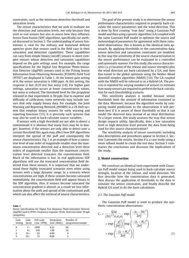
If sensors with a high threshold are not able to detect acontaminant it is obvious that many lives may be in dan-ger; however, if the sensors are only able to detect over acertain threshold this again may affect how SDF algorithmsinterpret the spread of the puff and consequently thesource characteristics. Fig. 1 is an example of how a satura-tion level of one order of magnitude smaller than the max-imum concentration detected and a detection level threeorders of magnitude smaller than the maximum concen-tration level detected truncates the concentration field.Much of the information is lost. In real applications SDFalgorithms will use the truncated concentration field de-tected from these sensors. It is important that we under-stand these highly truncated scenarios even when usingsensors with a large dynamic range. In a scenario whereconcentrations are high, if these sensors become saturatedimmediately, the concentration field will appear binary tothe SDF algorithm. Also, if sensors become saturated theconcentration gradient is altered; as a result we lose infor-mation about the path and spread of the contaminant puff,which can also affect the retrieval of source characteristics.

Table 1Sensor specifications for Digital Fast Response Photo-Ionization Detector(digiPID) used in FFT07. Frequency response: 50 Hz. Detection limit: 50 ppb(propylene).

Gainsetting

Gainfactor

Full scaleconc. (PPM)

Integrationtime (MSEC)

Number ofintegrations/sample

0 1� 1000 0.25 641 4� 250 1.00 162 16� 62 4.00 43 32� 31 8.00 2

The goal of the present study is to determine the sensorperformance characteristics required to properly back-cal-culate the source parameters and the wind direction. Thisis done by first creating ‘‘true data’’ using a Gaussian Puffmodel and then using a genetic algorithm (GA) coupled withthe same Gaussian Puff model to optimize the source andmeteorological parameters for agreement with these simu-lated observations: this is known as the identical twin ap-proach. By applying thresholds to the concentration data,sensor detection and saturation constraints are modeled.In this way the sensitivity of the source characterization tothe sensor performance can be evaluated in a controlledand systematic manner. For this study, the source character-istics (x, y) location of the release and source strength) plusthe wind direction are back-calculated by a GA, and thenfine-tuned to the global optimum using the Nelder–Meaddownhill simplex algorithm (NMDS) [16]. The GA coupledwith the NMDS will be referred to as a Hybrid GA. The pro-cess is repeated for varying numbers of sensors to estimatehow many sensors are required to perform the back-calcula-tion for each thresholding scenario.

This sensitivity analysis is needed because sensorthresholds limit the amount of information contained inthe data. Moreover, because the algorithm works by com-paring model predictions to the observations it will per-form best if it is aware of these thresholds so that it canmodel the observed data instead of an ideal distribution.To a larger extent, this study assesses the way that sensordesign impacts utility. Specifically, does a low saturationlevel or high detection level prevent the data from beingused for this source characterization?

The sensitivity analysis of sensor constraints includingdata descriptions and procedures appear in Section 2. Sec-tion 3 presents the results. Section 4 is a case study using amore refined model to create the test data. Section 5 sum-maries the conclusions and discusses the implications ofthe study.

2. Model construction

We construct an identical twin experiment with Gauss-ian Puff model output being used to back-calculate sourcestrength, location of the release, and wind direction. Wefirst describe how the concentration data is generated,then discuss the application of thresholds to the data tosimulate the sensor constraints, and finally describe theHybrid GA used to do the back-calculation.

2.1. The Gaussian Puff model

The Gaussian Puff model is used to produce the syn-thetic concentration observations:

Cr ¼QDt

ð2pÞ1:5rxryrz

exp�ðxr � UtÞ2

2r2x

!

� exp�y2

r

2r2y

!exp

�ðzr � HeÞ2

2r2z

!"

þ exp�ðzr þ HeÞ2

2r2x

!#ð1Þ

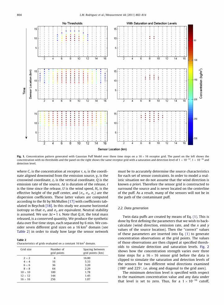
Fig. 1. Concentration pattern generated with Gaussian Puff Model over three time steps on a 16 � 16 receptor grid. The panel on the left shows theconcentration with no thresholds and the panel on the right shows the same receptor grid with a saturation and detection level of 1 � 10�12, 1 � 10�16 anddetection level.

804 L.M. Rodriguez et al. / Measurement 44 (2011) 802–814

where Cr is the concentration at receptor r, xr is the coordi-nate aligned downwind from the emission source, yr is thecrosswind coordinate, zr is the vertical coordinate, Q is theemission rate of the source, Dt is duration of the release, tis the time since the release, U is the wind speed, He is theeffective height of the puff center, and (rx, ry, rz) are thedispersion coefficients. These latter values are computedaccording to the fit by McMullen [17] with coefficients tab-ulated in Beychok [18]. In this study we assume horizontalisotropy so that rx and ry are equivalent. Neutral stabilityis assumed. We use Dt = 1 s. Note that QDt, the total massreleased, is a conserved quantity. We produce the syntheticdata over five time steps, each separated by 6 min. We con-sider seven different grid sizes on a 16 km2 domain (seeTable 2) in order to study how large the sensor network

Table 2Characteristics of grids evaluated on a constant 16 km2 domain.

Grid size Number ofgrid points

Spacing betweengrid points (km)

2 � 2 4 16.004 � 4 16 5.336 � 6 36 3.208 � 8 64 2.29

10 � 10 100 1.7812 � 12 144 1.4516 � 16 256 1.07

must be to accurately determine the source characteristicsfor each set of sensor constraints. In order to model a real-istic situation we do not assume that the wind direction isknown a priori. Therefore the sensor grid is constructed tosurround the source and is never located on the centerlineof the puff. As a result, many of the sensors will not be inthe path of the contaminant puff.

2.2. Data generation

Twin data puffs are created by means of Eq. (1). This isdone by first defining the parameters that we wish to back-calculate (wind direction, emission rate, and the x and yvalues of the source location). Then the ‘‘correct’’ valuesof these parameters are inserted into Eq. (1) to generateconcentration observations at the grid points. The valuesof those observations are then clipped at specified thresh-olds to simulate detection and saturation levels. Fig. 2shows how the concentration strength varies over threetime steps for a 16 � 16 sensor grid before the data isclipped to simulate the saturation and detection levels ofthe sensors for two different wind directions examined(180� and 225�, i.e. along and diagonal to the grid axes).

The minimum detection level is specified with respectto the maximum concentration value and any data underthat level is set to zero. Thus, for a 1 � 10�16 cutoff,

Fig. 2. Concentration pattern over three time steps on a 16 � 16 receptor grid. The panel on the left shows the concentration with a 180� wind direction andthe panel on the right for a 225� wind direction.

L.M. Rodriguez et al. / Measurement 44 (2011) 802–814 805

anything smaller than 1 � 10�16 of the maximum concen-tration is changed to 0.0, and similarly for the 1 � 10�12,1 � 10�8, 1 � 10�4, 1 � 10�3, 1 � 10�2, 1 � 10�1, 5 � 10�1,1 � 10�0 detection threshold levels. Saturation level is de-fined similarly for this study. Any value over a specifiedpercentage of the maximum concentration is clipped tothat level. For example, for a saturation level of 1 � 10�00

of the maximum concentration, 1.0 kg m�3 is used as thecutoff value but for a saturation of 5 � 10�1 of the maxi-mum concentration, 0.5 kg m�3 is the cutoff. Examples ofthe detection and saturation cutoff levels are provided inFig. 3 where the maximum concentration in this illustra-tion is 1 kg m�3. After the data is clipped it serves as our‘‘true observations’’.

2.3. Solution procedure

After our ‘‘true observations’’ are generated, we use theHybrid GA to back-calculate from them the source param-eters and the wind direction. The GA begins with a randompopulation of ‘‘first guess’’ values for these variables takenfrom the ranges shown in Table 3. These trial solutions,known as chromosomes, are used to predict the downwindcontaminant concentration via Eq. (1). The results are thencompared to our ‘‘true observations’’ by means of the costfunction:

cost function ¼P5

t¼1

ffiffiffiffiffiffiffiffiffiffiffiffiffiffiffiffiffiffiffiffiffiffiffiffiffiffiffiffiffiffiffiffiffiffiffiffiffiffiffiffiffiffiffiffiffiffiffiffiffiffiffiffiffiffiffiffiffiffiffiffiffiffiffiffiffiffiffiffiffiffiffiffiffiffiffiffiffiPTRr¼1ðlog10ðCr þ eÞ � log10ðRr þ eÞÞ2

qP5

t¼1

ffiffiffiffiffiffiffiffiffiffiffiffiffiffiffiffiffiffiffiffiffiffiffiffiffiffiffiffiffiffiffiffiffiffiffiffiffiffiffiffiffiffiffiffiPTRr¼1ðlog10ðRr þ eÞÞ2

qð2Þ

where Cr is the concentration as predicted by the disper-sion model given by (1), Rr is the observation data valueat receptor r, TR is the total number of receptors, and e isa constant added to avoid logarithms of zero. Thus, the costfunction is formulated to measure the difference (as an L2norm) of the log of the concentrations predicted with thetrial variables from those that are measured by the virtualsensors. The predictions are clipped in the same manner asthe ‘‘true observations’’ as described above.

GAs work by evaluating an initial population of trialsolutions via the cost function then selecting the highestranking individuals to reproduce, forming a new genera-tion of trial solutions by the GA operators of mating andmutation [19]. These ‘‘offspring’’ solutions are then evalu-ated in turn and the process iterates (Fig. 4). The real-val-ued chromosomes used for mating are determined by arank weighted roulette wheel selection [19]. The matingprocedure blends each of the parameter values of the origi-nal two chromosomes to create new chromosomes [9], andthen a fixed percentage of the population is subject tomutation. Mutation is needed to explore the complete

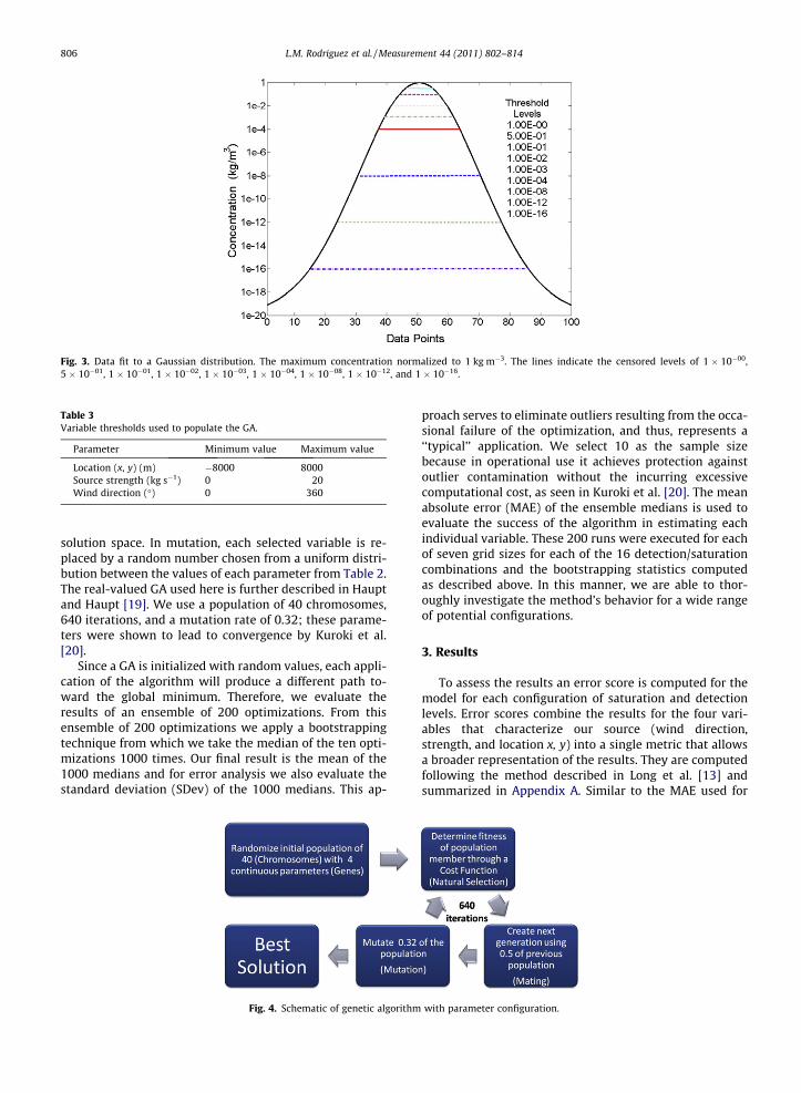
Fig. 3. Data fit to a Gaussian distribution. The maximum concentration normalized to 1 kg m�3. The lines indicate the censored levels of 1 � 10�00,5 � 10�01, 1 � 10�01, 1 � 10�02, 1 � 10�03, 1 � 10�04, 1 � 10�08, 1 � 10�12, and 1 � 10�16.

Table 3Variable thresholds used to populate the GA.

Parameter Minimum value Maximum value

Location (x, y) (m) �8000 8000Source strength (kg s�1) 0 20Wind direction (�) 0 360

806 L.M. Rodriguez et al. / Measurement 44 (2011) 802–814

solution space. In mutation, each selected variable is re-placed by a random number chosen from a uniform distri-bution between the values of each parameter from Table 2.The real-valued GA used here is further described in Hauptand Haupt [19]. We use a population of 40 chromosomes,640 iterations, and a mutation rate of 0.32; these parame-ters were shown to lead to convergence by Kuroki et al.[20].

Since a GA is initialized with random values, each appli-cation of the algorithm will produce a different path to-ward the global minimum. Therefore, we evaluate theresults of an ensemble of 200 optimizations. From thisensemble of 200 optimizations we apply a bootstrappingtechnique from which we take the median of the ten opti-mizations 1000 times. Our final result is the mean of the1000 medians and for error analysis we also evaluate thestandard deviation (SDev) of the 1000 medians. This ap-

Fig. 4. Schematic of genetic algorithm

proach serves to eliminate outliers resulting from the occa-sional failure of the optimization, and thus, represents a‘‘typical’’ application. We select 10 as the sample sizebecause in operational use it achieves protection againstoutlier contamination without the incurring excessivecomputational cost, as seen in Kuroki et al. [20]. The meanabsolute error (MAE) of the ensemble medians is used toevaluate the success of the algorithm in estimating eachindividual variable. These 200 runs were executed for eachof seven grid sizes for each of the 16 detection/saturationcombinations and the bootstrapping statistics computedas described above. In this manner, we are able to thor-oughly investigate the method’s behavior for a wide rangeof potential configurations.

3. Results

To assess the results an error score is computed for themodel for each configuration of saturation and detectionlevels. Error scores combine the results for the four vari-ables that characterize our source (wind direction,strength, and location x, y) into a single metric that allowsa broader representation of the results. They are computedfollowing the method described in Long et al. [13] andsummarized in Appendix A. Similar to the MAE used for

with parameter configuration.

L.M. Rodriguez et al. / Measurement 44 (2011) 802–814 807

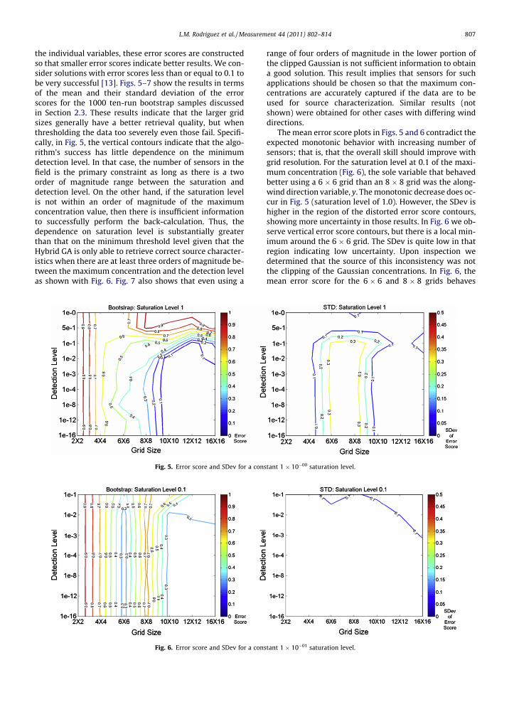
the individual variables, these error scores are constructedso that smaller error scores indicate better results. We con-sider solutions with error scores less than or equal to 0.1 tobe very successful [13]. Figs. 5–7 show the results in termsof the mean and their standard deviation of the errorscores for the 1000 ten-run bootstrap samples discussedin Section 2.3. These results indicate that the larger gridsizes generally have a better retrieval quality, but whenthresholding the data too severely even those fail. Specifi-cally, in Fig. 5, the vertical contours indicate that the algo-rithm’s success has little dependence on the minimumdetection level. In that case, the number of sensors in thefield is the primary constraint as long as there is a twoorder of magnitude range between the saturation anddetection level. On the other hand, if the saturation levelis not within an order of magnitude of the maximumconcentration value, then there is insufficient informationto successfully perform the back-calculation. Thus, thedependence on saturation level is substantially greaterthan that on the minimum threshold level given that theHybrid GA is only able to retrieve correct source character-istics when there are at least three orders of magnitude be-tween the maximum concentration and the detection levelas shown with Fig. 6. Fig. 7 also shows that even using a

Fig. 5. Error score and SDev for a cons

Fig. 6. Error score and SDev for a cons

range of four orders of magnitude in the lower portion ofthe clipped Gaussian is not sufficient information to obtaina good solution. This result implies that sensors for suchapplications should be chosen so that the maximum con-centrations are accurately captured if the data are to beused for source characterization. Similar results (notshown) were obtained for other cases with differing winddirections.

The mean error score plots in Figs. 5 and 6 contradict theexpected monotonic behavior with increasing number ofsensors; that is, that the overall skill should improve withgrid resolution. For the saturation level at 0.1 of the maxi-mum concentration (Fig. 6), the sole variable that behavedbetter using a 6 � 6 grid than an 8 � 8 grid was the along-wind direction variable, y. The monotonic decrease does oc-cur in Fig. 5 (saturation level of 1.0). However, the SDev ishigher in the region of the distorted error score contours,showing more uncertainty in those results. In Fig. 6 we ob-serve vertical error score contours, but there is a local min-imum around the 6 � 6 grid. The SDev is quite low in thatregion indicating low uncertainty. Upon inspection wedetermined that the source of this inconsistency was notthe clipping of the Gaussian concentrations. In Fig. 6, themean error score for the 6 � 6 and 8 � 8 grids behaves

tant 1 � 10�00 saturation level.

tant 1 � 10�01 saturation level.

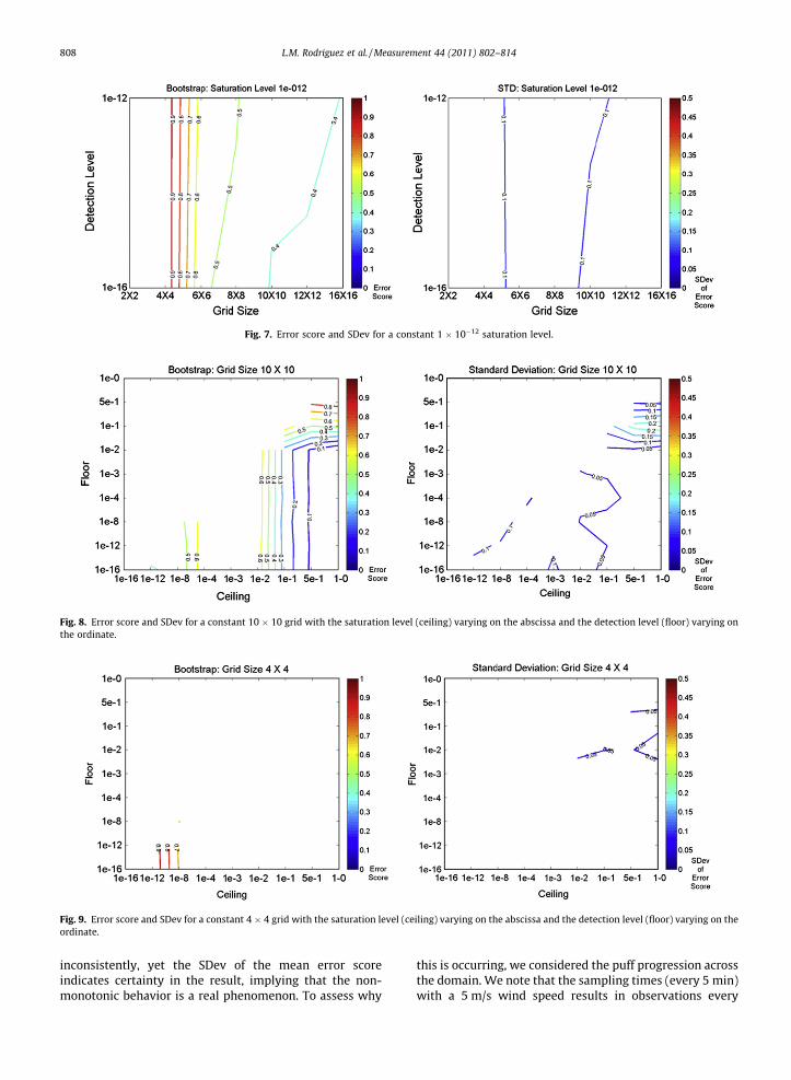
Fig. 7. Error score and SDev for a constant 1 � 10�12 saturation level.

Fig. 8. Error score and SDev for a constant 10 � 10 grid with the saturation level (ceiling) varying on the abscissa and the detection level (floor) varying onthe ordinate.

Fig. 9. Error score and SDev for a constant 4 � 4 grid with the saturation level (ceiling) varying on the abscissa and the detection level (floor) varying on theordinate.

808 L.M. Rodriguez et al. / Measurement 44 (2011) 802–814

inconsistently, yet the SDev of the mean error scoreindicates certainty in the result, implying that the non-monotonic behavior is a real phenomenon. To assess why

this is occurring, we considered the puff progression acrossthe domain. We note that the sampling times (every 5 min)with a 5 m/s wind speed results in observations every

L.M. Rodriguez et al. / Measurement 44 (2011) 802–814 809

1800 m, which is roughly half the grid spacing (3200 m) forthe 6 � 6 grid; therefore, the sampling times for the 6 � 6grid resulted in observing the puff every other samplingtime, but it observed the same portion of the puff. In con-trast, the sampling in the 8 � 8 grid was at about 80% ofthe spacing (2286 m) resulting in observing different por-tions of the puff each sampling time, which caused an incor-rect estimate of the along-wind direction variable, y. Given

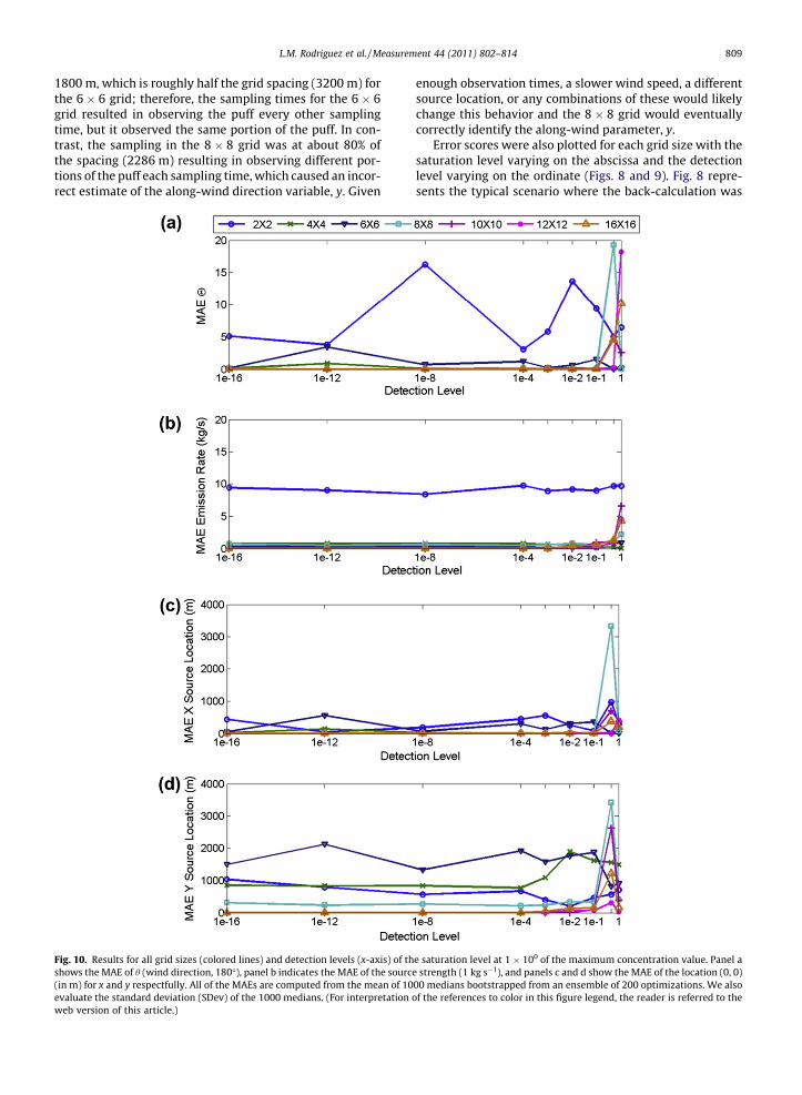
Fig. 10. Results for all grid sizes (colored lines) and detection levels (x-axis) of thshows the MAE of h (wind direction, 180�), panel b indicates the MAE of the sourc(in m) for x and y respectfully. All of the MAEs are computed from the mean of 10evaluate the standard deviation (SDev) of the 1000 medians. (For interpretationweb version of this article.)

enough observation times, a slower wind speed, a differentsource location, or any combinations of these would likelychange this behavior and the 8 � 8 grid would eventuallycorrectly identify the along-wind parameter, y.

Error scores were also plotted for each grid size with thesaturation level varying on the abscissa and the detectionlevel varying on the ordinate (Figs. 8 and 9). Fig. 8 repre-sents the typical scenario where the back-calculation was

e saturation level at 1 � 100 of the maximum concentration value. Panel ae strength (1 kg s�1), and panels c and d show the MAE of the location (0, 0)00 medians bootstrapped from an ensemble of 200 optimizations. We alsoof the references to color in this figure legend, the reader is referred to the

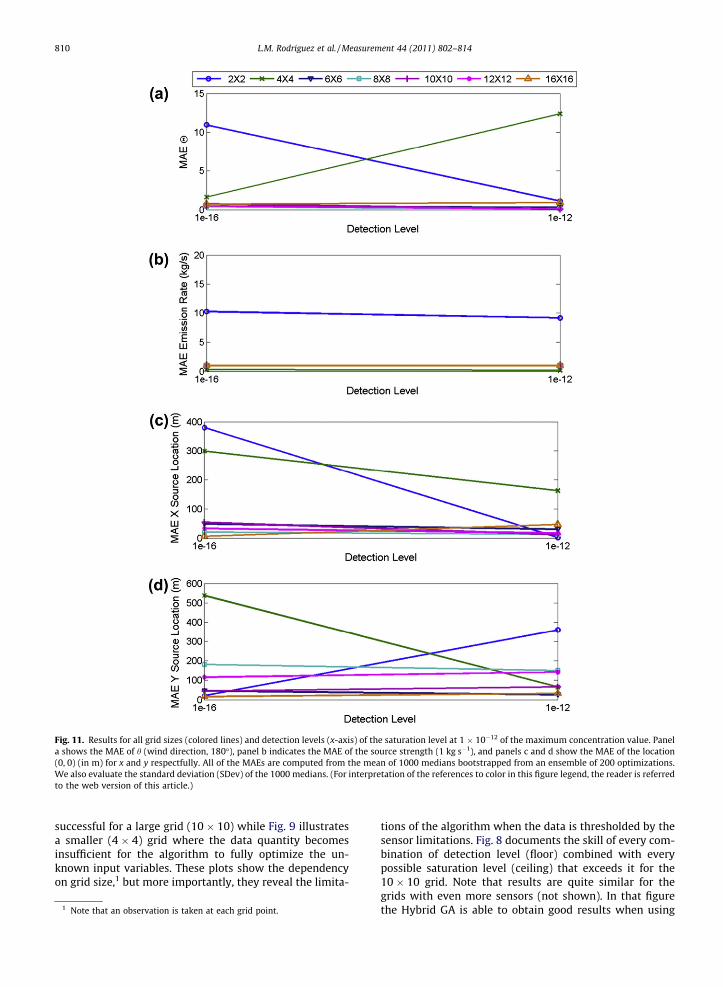
Fig. 11. Results for all grid sizes (colored lines) and detection levels (x-axis) of the saturation level at 1 � 10�12 of the maximum concentration value. Panela shows the MAE of h (wind direction, 180�), panel b indicates the MAE of the source strength (1 kg s�1), and panels c and d show the MAE of the location(0, 0) (in m) for x and y respectfully. All of the MAEs are computed from the mean of 1000 medians bootstrapped from an ensemble of 200 optimizations.We also evaluate the standard deviation (SDev) of the 1000 medians. (For interpretation of the references to color in this figure legend, the reader is referredto the web version of this article.)

810 L.M. Rodriguez et al. / Measurement 44 (2011) 802–814

successful for a large grid (10 � 10) while Fig. 9 illustratesa smaller (4 � 4) grid where the data quantity becomesinsufficient for the algorithm to fully optimize the un-known input variables. These plots show the dependencyon grid size,1 but more importantly, they reveal the limita-

1 Note that an observation is taken at each grid point.

tions of the algorithm when the data is thresholded by thesensor limitations. Fig. 8 documents the skill of every com-bination of detection level (floor) combined with everypossible saturation level (ceiling) that exceeds it for the10 � 10 grid. Note that results are quite similar for thegrids with even more sensors (not shown). In that figurethe Hybrid GA is able to obtain good results when using

L.M. Rodriguez et al. / Measurement 44 (2011) 802–814 811

a saturation level of 1 � 10�00 and 5 � 10�01 in conjunctionwith any detection level lower than 1 � 10�02. As thedetection level increases, the scenario loses informationwith the limiting case being that of a binary sensor repre-sented by the diagonal. As the scenario approaches the bin-ary case, we see a breakdown in skill. Fig. 9 plots results forthe 4 � 4 grid, the first resolution at which results begin todegrade. The breakdown in skill for all ceiling and floorcombinations is evident, but even in this case, some skillexists for the largest dynamic ranges.

Figs. 10 and 11 plot the aforementioned MAE values foreach of the solution variables so that we can further ana-lyze the results. Each figure reflects a specific saturation le-vel (full maximum of 1 � 10�01 in Fig. 10 and 1 � 10�12 forFig. 11) while varying detection levels appear across the

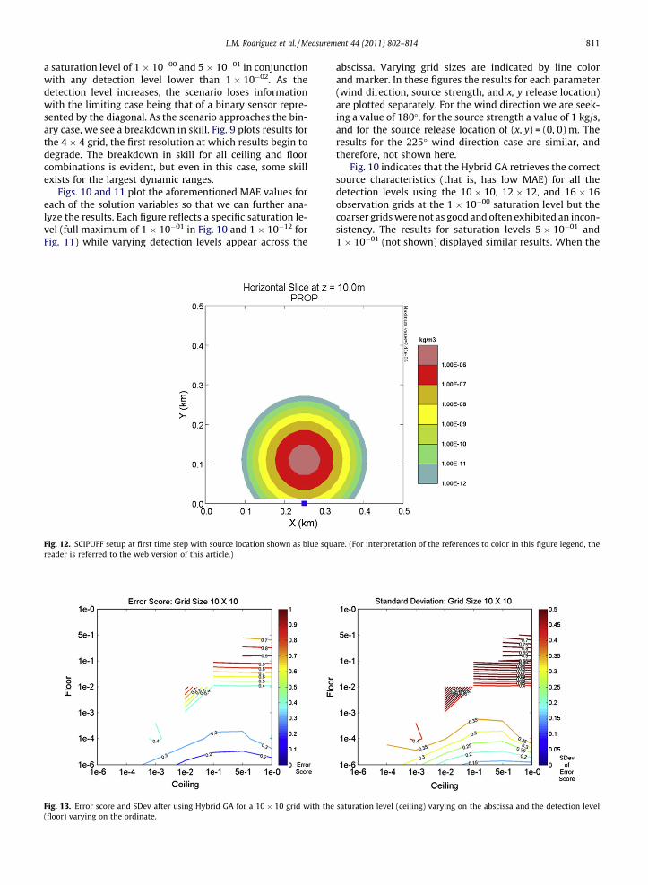
Fig. 12. SCIPUFF setup at first time step with source location shown as blue squreader is referred to the web version of this article.)

Fig. 13. Error score and SDev after using Hybrid GA for a 10 � 10 grid with the(floor) varying on the ordinate.

abscissa. Varying grid sizes are indicated by line colorand marker. In these figures the results for each parameter(wind direction, source strength, and x, y release location)are plotted separately. For the wind direction we are seek-ing a value of 180�, for the source strength a value of 1 kg/s,and for the source release location of (x, y) = (0, 0) m. Theresults for the 225� wind direction case are similar, andtherefore, not shown here.

Fig. 10 indicates that the Hybrid GA retrieves the correctsource characteristics (that is, has low MAE) for all thedetection levels using the 10 � 10, 12 � 12, and 16 � 16observation grids at the 1 � 10�00 saturation level but thecoarser grids were not as good and often exhibited an incon-sistency. The results for saturation levels 5 � 10�01 and1 � 10�01 (not shown) displayed similar results. When the

are. (For interpretation of the references to color in this figure legend, the

saturation level (ceiling) varying on the abscissa and the detection level

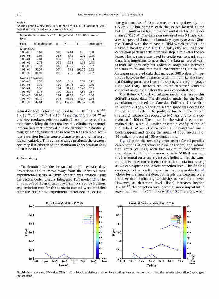
Table 4GA and Hybrid GA MAE for a 10 � 10 grid and a 1.0E�00 saturation level.Note that the error values here are not bound.

Mean absolute error for a 10 � 10 grid and a 1.0E�00 saturationlevel

Floor Wind direction Q X Y Error score

GA solutions1.0E�00 1.68 0.89 12.64 1.90 0.085.0E�01 0.95 0.88 5.41 2.02 0.051.0E�01 2.03 0.82 9.37 17.79 0.031.0E�02 2.74 0.76 17.33 1.13 0.031.0E�03 13.37 0.80 35.25 3.27 0.071.0E�04 53.57 0.74 7.02 191.25 0.521.0E+08 80.91 0.73 7.15 209.13 0.57

Hybrid GA solutions1.0E�00 0.57 0.93 3.11 0.62 0.125.0E�01 3.79 1.02 24.14 2.65 0.401.0E�01 7.91 1.01 37.63 28.48 0.391.0E�02 9.78 1.00 59.31 1.82 0.371.0E�03 180.82 1.01 47.23 0.43 0.961.0E�04 45.10 0.71 96.86 84.57 0.641.0E+08 142.64 0.72 152.40 102.67 0.68

812 L.M. Rodriguez et al. / Measurement 44 (2011) 802–814

saturation level is further reduced to 1 � 10�02, 1 � 10�03,1 � 10�04, 1 � 10�08, 1 � 10�12 (see Fig. 11), 1 � 10�16 nogrid size produces reliable results. These findings confirmthat thresholding the data too severely eliminates so muchinformation that retrieval quality declines substantially:thus, greater dynamic range in sensors leads to more accu-rate inversion for the source characteristics and meteoro-logical variables. This dynamic range produces the greatestaccuracy if it extends to the maximum concentration as isillustrated in Fig. 7.

4. Case study

To demonstrate the impact of more realistic datalimitations and to move away from the identical twinexperimental setup, a 5 min scenario was created usingthe Second-order Closure Integrated Puff model [21]. Thedimensions of the grid, quantity of sensors, source location,and emission rate for the scenario created were modeledafter the FFT07 field experiment introduced in Section 1.

Fig. 14. Error score and SDev after GA for a 10 � 10 grid with the saturation levelthe ordinate.

The grid consists of 10 � 10 sensors arranged evenly in a0.5 km � 0.5 km domain with the source located at thebottom (southern edge) in the horizontal center of the do-main at (0.25, 0). The emission rate used was 0.1 kg/s witha wind speed of 2 m/s, the boundary layer type was a Sim-ple Diurnal with the release at 3PM which produces anunstable stability class. Fig. 12 displays the resulting con-centration pattern at the first time step, 1 min after the re-lease. This scenario was used to create our concentrationdata. It is important to note that the data generated withSCIPuff includes only six orders of magnitude betweenthe maximum and minimum concentrations, unlike theGaussian generated data that included 300 orders of mag-nitude between the maximum and minimum, i.e. the inter-nal floating point precision of the programming languageused (MATLAB). The tests are limited to sensor floors sixorders of magnitude below the peak concentrations.

Our Hybrid GA back-calculation model was run on thisSCIPuff-created data. The dispersion model for the back-calculation remained the Gaussian Puff model describedin Section 2. The GA solution search space was decreasedto match the needs of the problem: for the emission ratethe search space was reduced to 0–5 kg/s and for the do-main to 0–500 m. The range for the wind direction re-mained the same. A similar ensemble configuration ofthe Hybrid GA with the Gaussian Puff model was run –bootstrapping and taking the mean of 1000 medians of10 realizations out of 100 optimizations.

Fig. 13 plots the resulting error scores for all possiblecombinations of detection thresholds (floors) and satura-tion limits (ceilings) with the maximum concentrationnormalized to 1. In this more realistic SCIPuff scenariothe horizontal error score contours indicate that the satu-ration level does not influence the back-calculation as longas we can capture the lowest detection level. This findingcontrasts to the results shown in the comparable Fig. 8,where for the smallest detection levels the contours weremore vertical, indicating sensitivity to saturation level.However, as detection level (floor) increases beyond1 � 10�02, the detection level becomes more important inagreement with this SCIPuff case (Fig. 13). Therefore, when

(ceiling) varying on the abscissa and the detection level (floor) varying on

L.M. Rodriguez et al. / Measurement 44 (2011) 802–814 813

using more realistic data with a lower dynamic range, themost important feature to capture is the spread of the puff,which is revealed by the full range of concentrations. Thisfinding supports the conclusion above that having accessto the largest available dynamic range enhances the abilityof our algorithm to estimate the source term.

We note, however, that the error score values in Fig. 13are substantially higher than for the identical twin case ofFig. 8. In fact, upon further examination, we establishedthat the NMDS algorithm produced a worse solution thanthe GA alone. Table 4 lists the MAEs for each individualvariable as well as the error scores for each detection levelmaintaining a constant saturation level of 1 � 10�00 forboth the GA alone and the Hybrid GA that includes theNMDS. For this case study, the GA alone produces muchbetter results (lower MAEs and lower error scores) thanwhen the NMDS is included. The NMDS algorithm doesnot allow specific bounds on the variables; therefore, weoften obtained solutions that were out of our domain.Fig. 14 depicts the error scores when only the GA was used.It is obvious that the detection level becomes lessimportant in agreement with our identical twin results.This analysis indicates that it may be more appropriateto apply only the GA for mixed model applications.

5. Conclusions

This study has sought to determine to what extent sen-sor thresholds limit the feasibility of back-calculatingsource characteristics and wind direction from sensor fieldmeasurements. It has augmented the literature on sourceterm estimation for CBRN data by considering the impactof more realistic sensor characteristics. The Hybrid GAmethod used here (with NMDS) is successful in back-calcu-lating source characteristics and wind direction with iden-tical twin data that has been thresholded to includedetection limits and saturation levels. These thresholds, iftoo restrictive, eliminate so much information that retrie-val quality degrades severely. The identical twin experi-ments indicate that inversion is most successful if eachsensor can detect the maximum concentrations (ie. has ahigh saturation level), which means that the most effectivesensors have this characteristic. The case study using SCI-Puff to generate the sensor data demonstrates that onemust be careful in applying algorithms to different datatypes. In fact, the GA alone produced better results thanthe Hybrid GA that includes the NMDS. For such cases ofdiffering data types, it is critical to use a very robust opti-mization method that does not rely on a good first guesssolution. For sensor data inversion using the Gaussianmodel with GA optimization both sensor detection and sat-uration limits are equally important. In contrast, when theSCIPuff model is used with GA optimization the detectionlimit is more important. Thus, for the Gaussian model sen-sor dynamic range is the key to success while for SCIPuffboth dynamic range and a detection threshold low enoughto sample the puff periphery are essential. In conclusion, itis important to select an accurate optimization techniqueas well as model saturation and detection levels in sensors,

specifically when using a GA coupled with an AT&D modelto estimate source parameters.

This work demonstrates that it is important that thesensors have sufficient dynamic range in order to use thedata effectively for source term estimation. From the casestudy results using SCIPuff, we see that the necessary rangevaries according to the problem. In addition, a sufficientnumber of sensors must be available to define the center-line and spread of the plume. Once again, having the fullrange of concentrations allows the algorithm to betterquantify the unknown source variables. However, a robustalgorithm (such as a GA) still shows skill when the dy-namic range is reduced.

This work modeled generic sensor characteristics ratherthan emulating any particular sensor in order to retain gen-erality. It points out the importance of considering sensorcharacteristics when developing new numerical techniquesthat use their data. It also demonstrates that informationneeds of the intended retrieval mission must be consideredwhen specifying sensors for a monitoring network. Studiessuch as this one that use known modeled solutions as inputdata are an important step since this approach allows sepa-ration of the sensor characteristics from other sources of er-ror, including sensor calibration, atmospheric turbulence,and inadequacies of the atmospheric transport and disper-sion models. Such considerations should be included in fu-ture work. Of particular interest is whether higherfrequency sampling would improve our ability to compen-sate for lack of dynamic range. Note that typical sensorssample at a sufficient frequency to detect the puff or plume.To sample more frequently would only further resolve thenoise and would therefore not be helpful.

The results demonstrated here should be confirmedwith concentration data measured during a field experi-ment and we are currently assessing these issues usingthe FFT07 data. We note that this current study uses a sin-gle method for source characterization to assess the sensorconstraints. Other methods should also be consideredwhen evaluating the limits of sensor usage.

Note that one can also assimilate the available sensordata directly into atmospheric transport and dispersionmodels or, equivalently, apply sensor data fusion to thosemodels to improve contaminant concentration predictionswithout recovering source information [22,23]. Such workis complementary to the current study. In fact, one can viewthe methods presented here as an example of using sensordata fusion techniques to retrieve the source parameters.

In summary, the current study indicates the importanceof designing sensor networks for chem-bio applicationswith knowledge of the sensor constraints and of how thoseconstraints will limit the future use of their data. Addition-ally, algorithms that use such data must be designed withknowledge of those constraints to prevent failure in a real-istic situation. For FFT07 we will use the lessons learned toimplement sensor noise thresholds.

Acknowledgements

This work was supported by the Defense ThreatReduction Agency under Grants W911NF-06-C-0162,01-03-D-0010-0012, and by the Bunton–Waller Fellowship.

814 L.M. Rodriguez et al. / Measurement 44 (2011) 802–814

Support for professional development was supplied bythe Significant Opportunities in Atmospheric Researchand Science Program. Dr. Randy L. Haupt provided theframework for the genetic algorithm and Christopher Allenand Kerrie Long contributed to the source characterizationcode. We would like to thank Kerrie Long, Dave Swanson,Arthur Small, Anke Beyer-Lout, Andrew Annunzio, andYuki Kuroki for helpful discussions. Finally, we thank twoanonymous reviewers for some very helpful comments thathelped us refine our analysis and strengthen our results.

Appendix A. Definition of error scores

The error score is used to assess the accuracy of thesolutions found by the GA and the Nelder–Mead search.The ‘‘error’’ is based on the following equations.

Eloc ¼ 1:25� 10�4 � dist ðA:1Þ

Edir ¼ minððjhfou � hactjÞ; ð360� jhfou � hactjÞÞ=90 ðA:2Þ

Estr ¼ maxEact � Efou

Eact � Emin

� �;

Efou � Eact

Emax � Eact

� �� �ðA:3Þ

where dist is the distance between the GA computedsource location and the actual source location, (0, 0), inmeters, hfou is the wind direction found by the GA, hact isthe actual wind direction, 180�, Eact is the actual sourcestrength of 1.0 kg/s, Efou is the strength found by the GA,Emin and Emax are the minimum and maximum values allot-ted for the GA described in Table 2.

Each parameter is normalized on a scale of [0, 1], where1 is the absolute worst possible solution and 0 is the best.The final error score is the mean of the Eloc, Edir,and Estr. Theerror scores are evaluated with the results from only theGA and then with results from the Hybrid GA. It is impor-tant to note that the Hybrid GA is not bound and the errorscore may give us a value large than 1, however in thiswork we bound the error between 0 and 1.

References

[1] Homeland Security Office, National Strategy for Homeland Security,2007. <http://www.whitehouse.gov/infocus/homeland/nshs/NSHS.pdf>.

[2] National Research Council, Tracking and Predicting the AtmosphericDispersion of Hazardous Material Releases. Implications forHomeland Security. The National Academies Press, 2003, 114 pp.

[3] Defence Research and Development Canada, CRTI-IRTC AnnualReport 2005–2006, ISSN 1912-0974. <http://www.css.drdc-rddc.gc.ca/crti/publications/reports-rapports/ar05_06_pt1-eng.pdf>.

[4] European Union Committee, Preventing Proliferation of Weapons ofMass Destruction: The EU Contribution. Report with Evidence, Houseof Lords, the Stationery Office Limited, London, 2005. <http://www.parliament.the-stationery-office.co.uk/pa/ld200405/ldselect/ldeucom/96/96.pdf>.

[5] L.C. Thomson, B. Hirst, G. Gibson, S. Gillespie, P. Jonathan, K.D.Skeldon, M.J. Padgett, An improved algorithm for locating a gassource using inverse methods, Atmospheric Environment 41 (2007)1128–1134.

[6] S. Rao, Source estimation methods for atmospheric dispersion,Atmospheric Environment 41 (2007) 6963–6973.

[7] S.E. Haupt, A demonstration of coupled receptor/dispersionmodeling with a genetic algorithm, Atmospheric Environment 39(2005) 7181–7189.

[8] S.E. Haupt, G.S. Young, C.T. Allen, Validation of a receptor/dispersionmodel with a genetic algorithm using synthetic data, Journal ofApplied Meteorology 45 (2006) 476–490.

[9] C.T. Allen, G.S. Young, S.E. Haupt, Improving pollutant sourcecharacterization by optimizing meteorological data with a geneticalgorithm, Atmospheric Environment 41 (2006) 2283–2289.

[10] C.T. Allen, S.E. Haupt, G.S. Young, Source characterization with areceptor/dispersion model coupled with a genetic algorithm,Journal of Applied Meteorology and Climatology 46 (2007) 273–287.

[11] S.E. Haupt, G.S. Young, C.T. Allen, A genetic algorithm method toassimilate sensor data for a toxic contaminant release, Journal ofComputers 2 (2007) 85–93.

[12] S.E. Haupt, R.L. Haupt, G.S. Young, A mixed integer genetic algorithmused in chem-bio defense applications, Journal of Soft Computing 15(2011) 51–59.

[13] K.J. Long, S.E. Haupt, G.S. Young, Assessing sensitivity of source termestimation, Atmospheric Environment 44 (2010) 1558–1567.

[14] FUsing Sensor Information from Observing Networks (FUSION) FieldTrial 2007 (FFT07), 2010. <https://www.fft07-slc.org/>.

[15] John Hannan, Senior Science and Technology Manager – Warning,Reporting, Information and Analysis at the US Defense ThreatReduction Agency Joint Science & Technology Office for Chemicaland Biological Defense, personal communication, 2010.

[16] J.A. Nelder, R. Mead, A simplex method for function minimization,Computer Journal 7 (1965) 308–313.

[17] R.W. McMullen, The change of concentration standard deviationswith distance, Journal of the Air Pollution Control Association(October) (1975).

[18] M.R. Beychok, Fundamentals of Gas Stack Dispersion, third ed.,Milton Beychok, Pub., Irvine, CA, 1994.

[19] R.L. Haupt, S.E. Haupt, Practical Genetic Algorithms, Wiley, 2004.[20] Y. Kuroki, G.S. Young, S.E. Haupt, UAV navigation by an expert

system for contaminant mapping with a genetic algorithm, ExpertSystems with Applications 37 (2010) 4687–4697.

[21] R.I. Sykes, S.F. Parker, D.S. Henn, SCIPUFF Version 2.0, TechnicalDocumentation. ARAP Tech. Rep. 727, Titan Corp., Princeton, NJ,2004, 284 pp.

[22] G. Andria, G. Cavone, A.M.L. Lanzolla, Modelling study forassessment and forecasting variation of urban air pollution,Measurement 41 (2008) 222–229.

[23] K.V.U. Reddy, Y. Cheng, T. Singh, P.D. Scott, Data assimilation invariable dimension dispersion models using particle filters, in: The10th International Conference on Information Fusion, Quebec,Canada, 2007.