


Bahasa
Halaman
Hukum


HFSS SIMULATION OF NEAR-FIELD BEAM FORMING USING S-BAND RECTANGULAR HORN ANTENNA ARRAY FOR HYPERTHERMIA THERAPY
APPLICATIONS
Dhara Kiritkumar Trivedi B.E, Gujarat University, India, 2006
Thomas D Jerome-Surendran B.E, Anna University, India, 2005
PROJECT
Submitted in partial satisfaction of the requirements for the degree of
MASTER OF SCIENCE
in
ELECTRICAL AND ELECTRONIC ENGINEERING
at
CALIFORNIA STATE UNIVERSITY, SACRAMENTO
FALL 2009
ii
HFSS SIMULATION OF NEAR-FIELD BEAM FORMING USING S-BAND
RECTANGULAR HORN ANTENNA ARRAY FOR HYPERTHERMIA THERAPY APPLICATIONS
A Project
by
Dhara Kiritkumar Trivedi
Thomas D Jerome-Surendran Approved by: __________________________________, Committee Chair Dr.Preetham B. Kumar __________________________________, Second Reader Dr.Jing Pang ___________________________ Date

iii
Students: Dhara Kiritkumar Trivedi Thomas D Jerome-Surendran
I certify that these students have met the requirements for format contained in the
University format manual, and that this project is suitable for shelving in the Library and
credit is to be awarded for the Project.
___________________, Graduate Coordinator ____________ Dr.Preetham B. Kumar Date
Department of Electrical and Electronic Engineering

iv
Abstract
of
HFSS SIMULATION OF NEAR-FIELD BEAM FORMING USING S-BAND RECTANGULAR HORN ANTENNA ARRAY FOR HYPERTHERMIA THERAPY
APPLICATIONS
by
Dhara Kiritkumar Trivedi and Thomas D Jerome-Surendran
The focus of this project is to carry out an accurate simulation study of a 3- element array
of rectangle horn antennas forming a focused near field beam. This study has useful
application for clinical hyperthermia which is the therapeutic treatment of tumors in the
body by heating caused by focused RF or microwave radiation. This principle of
treatment is proved to be very useful for cancer treatment usually in conjunction with
traditional radiation or chemotherapy, and can even double the tumor response rate as
compared to radiation alone.. The 3-element array set up consists of a central focusing
element and two surrounding directing elements. The focusing element can be axially
adjusted and surrounding elements are fixed to focus the beam of a required point, which
is necessary in hyperthermia treatment. In this project the simulation results were
obtained from ANSOFT HFSS simulations.
, Committee Chair Dr.Preetham B. Kumar ______________________ Date
v
ACKNOWLEDGEMENT Man has made language to express his feelings. Yet, we find ourselves short of words
when it comes to thanking all those who have rendered necessary help for the completion
of this project.
First and foremost we would like to express our gratitude and thanks to our advisor,
committee chair and graduate coordinator Dr. Preetham Kumar for his expert guidance
and constant support throughout this project. His openness and enthusiasm have taught us
correct way of working with new technologies and have improved our knowledge of the
subject. Also, his constant vigilance with the right amount of freedom, not only as a
project guide but as a guardian too.
We are extremely thankful to Dr. Jing Pang, our second reader, for reviewing this work
and for her valuable suggestions in improving the same. It is our duty to recognize the
efforts of Electrical Engineering Department and the management for creating an
interactive atmosphere for learning.
We would also like to take this opportunity to thank the considerate faculty and staff of
Electrical and Electronics Engineering Department who have been encouraging us
through out our curriculum.
At the end we would like to extend our thanks to our parents for their constant
encouragement and to all those who have played a small but important role in this project
but could not be individually named here.
vi
TABLE OF CONTENTS Page Acknowledgement………………………………………………………………………..v List of Tables…………………………………………………………………………….vii List of Figures……………………………………………………………………...…...viii
Chapter
1. INTRODUCTION ......................................................................................................... 1 2. ANSOFT HIGH FREQUENCY STRUCTURE SIMULATOR ................................... 3
2.1 Introduction to HFSS ................................................................................................ 3 2.2 Theory behind HFSS High Freuency Structure Simulator……………..…...……...4 2.3 Finite Element Method (FEM) Software…………..………………..……………...4 2.4 FEM Problem Constraints………………………………………………………….5
2.5 Ansoft HFSS Project Flow..………………………………………………………..5 2.6 Configuration and Accessing Project Manager………………………………….....6
2.8 Command and Display Area………………………………………………………..8 2.9 Steps for drawing geometric model ........................................................................ 10
3. INFORMATION ABOUT HYPERTHERMIA ........................................................... 14
3.1 Causes of Hyperthermia .......................................................................................... 14 3.2 Meaning of Hyperthermia ....................................................................................... 14 3.3 Methodology for Hyperthermia Treatment ............................................................. 15 3.4 Types of Hyperthermia……………….……………..………………………….…15
3.5 Types of Hyperthermia Treatment…………………………..…………………….17 3.6 Side effects of Hyperthermia………...……………………………………………18 3.7 Future scope for Hyperthermia …………………………………………………...18 4. DESIGN AND SET UP OF S BAND RECTANGULAR HORN ARRAY. ............... 19
4.1 Measurement of near-field of single horn Antenna along the axis of the antenna .. 20 4.2 Measurement of Z axis near-field of 3element horn antenna array. ........................ 21 4.3 Experimental Characterization of current distribution in the feed network……..…….25
5. SIMULATION RESULTS OF S BAND RECTANGULAR HORN ARRAY……....26 5.1 HFSS setup, simulation and array parameters……….…………………………….26 5.2 HFSS simulation with new parameter…………...……………………...…………34 6. CONCLUSION AND SCOPE FOR FUTURE WORK ............................................... 40 References ......................................................................................................................... 41

vii
LIST OF TABLES
1. Table 5.1 Comparison of Measured and Simulated data……………………………38
viii
LIST OF FIGURES
1. Figure 2.1 Ansoft HFSS Project Manager………......................…………………….....7
2. Figure 2.2 Command Window…….. …………….………………………….……......8
3. Figure 2.3 Flow Chart for simulation in Ansoft HFSS………….…………...…..........9
4. Figure 2.4 3D Modeler Window…………………………………………….……..... 10
5. Figure 2.5 3D View of Geometric Model……………………..……...………..……. 11
6. Figure 2.6 3D view of HFSS solution setup window.....………………....…………. 12
7. Figure 2.7 E and H Field Pattern in HFSS..……………....…………………………. 12
8. Figure 2.8 Post progressing far field…………………………...………………..….. 13
9. Figure 4.1 Photograph of 3 element horn array set up in lab…………………….…..19
10. Figure 4.2 Experimental setup for single-element antenna…..…………….;………20 11. Figure 4.3 Axial near zone electric field of single horn antenna………..…………...21 12. Figure 4.4 Experimental setup for 3-element horn array with 3 elements in line.......22 13. Figure 4.5 Experimental setup for 3-element horn array with central element 5.08 cm
behind outer directing elements……………………………………………………...23 14. Figure 4.6 Experimental setup for 3-element horn array with central element 10.16cm
behind outer directing elements…………………………………………………..….24 15. Figure 4.7 Consolidated beam focusing demonstration for 3-element horn array .....25
16. Figure 5.1a HFSS Schematic when all elements are in line………………...…….…27
17. Figure 5.1b Electric field along a XY plane at the highest field point………….…...28
18. Figure 5.1c Near Field pattern (actual distance= 30 cm) all horn antennas are in line…............................................................................................................................28
19. Figure 5.2a HFSS schematic when all elements are in line……………….……..…..29
ix
20. Figure 5.2b Electric field along a XY plane at the highest field point…….…..….....30
21. Figure 5.2c Near field pattern (actual distance = 30 cm) center element is 5 cm behind the other two elements………………………………………………………...……..31
22. Figure 5.3a HFSS schematic when all elements are in line………………………....32
23. Figure 5.3b Electric field along a XY plane at the highest field point…….………..33
24. Figure 5.3c Near field pattern (actual distance = 30 cm) center element is 10 cm behind the other two elements…………………………………………………….....34
25. Figure 5.4a Near field pattern (actual distance = 30 cm) all elements are in line.…..35
26. Figure 5.4b Near field pattern (actual distance = 30 cm) center element is 5cm behind the other two elements……………………………………………………………….36
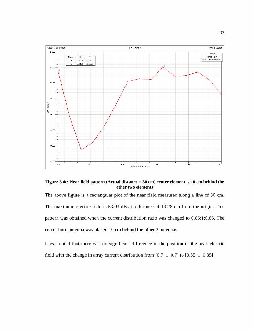
27. Figure 5.4c Near field pattern (actual distance = 30 cm) center element is 10 cm
behind the other two elements…………………………………………………….....37
1
Chapter 1
INTRODUCTION
Microwaves are short electromagnetic waves with short wavelength. A credible
definition comes from Pozar's text "Microwave Engineering" [10], which states that the
term microwave "refers to alternating current signals with frequencies between 300 MHz
(3 x 10⁸ Hz) and 300 GHz (3 x 10¹¹ Hz). However, the boundaries between far infrared
light, microwaves, and ultra-high-frequency radio waves are fairly arbitrary and are used
variously between different fields of study. Due to its unique characteristics microwave
components are used in a variety of applications in today’s world. From communications
to imaging, remote sensing, heating methods, microwaves have been used in a variety of
ways to suit the ever growing demands of the industry. Along with such widespread
applications, microwaves are also used in certain niche applications. One such
application is the use of microwaves for medical diagnostic and treatment. This area of
research has been quietly gathering pace and has been moving slowly but steadily
towards solving the growing needs of medical science.
The microwave electric field has two main components associated with it: the first
one, known as Far Field, is used in communication systems. The second component,
known as Near Field, has applications primarily targeting the medical imaging & therapy
techniques.
Microwave Hyperthermia is a very important near field component of
Electromagnetic energy, and the S-band frequency range of 2.45 GHz is found to be very

2
suitable for heat absorption [1]. Hyperthermia is a form of treatment given to cure the
tumors in different parts of body. The tumor area is heated to therapeutic temperatures of
about 42°C, without over-heating the surrounding normal tissues. Special care and
intense sharp beam focus is required in order to avoid the heat radiation in surrounding of
the tumor. This is the point where accurate antenna setup and formation of conformal
microwave antenna radiation is required.
The aim of this project is the theoretical study of a 3-element array of rectangular
horn antennas, operating in the S-band frequency range of 2.45 GHz. The aim of the
array is to obtain a beam focus at a prescribed point in the near field of the array. The
array also has the ability to move the focus point along the axial direction of the array by
adjusting the position of the central focusing element of the array. The theoretical
simulations are done using Ansoft High Frequency Structure Simulator (HFSS).
The report is organized as follows: Chapter 1 is an introduction. Chapter 2
describes the Ansoft HFSS software. Chapter 3 explains background on clinical
hyperthermia. Chapter 4 gives details of the three-element array simulation for different
focusing points along the axis of the array. Chapter 5 gives conclusions from the results
obtained and direction for future work, followed with the references.
3
Chapter 2
ANSOFT HIGH FREQUENCY STRUCTURE SIMULATOR
2.1 Introduction to HFSS
Ansoft High Frequency Structure Simulator (HFSS) is interactive software that
allows you to characterize full wave and radioactive effects for passive high frequency
transmission structures. Using finite element based solvers. We used Ansoft HFSS ver.
11 which is allows you to compute and view the following:
• Basic Electromagnetic Field quantities, antenna parameters, and for open
boundary problems, radiated fields.
• characteristic port impedance and propagation constants
• Generalized S-parameters and S-parameters renormalized to specific port
impedances.
You are expected to draw the structure, specify material characteristic for each
object and identify ports, sources and special surface characteristics. The system then
generates the necessary field solutions. As you setup the problem HFSS allows you to
specify whether to solve the problem at one specific frequency or at several frequencies
within a range.
Ansoft HFSS ver. 11 is available on UNIX workstations running X windows and
personal computers running Windows NT. The version available at CSU Sacramento is
available on Windows. In HFSS, the geometric model is automatically divided into a
large number of tetrahedral, where a single tetrahedron is basically a four-sided pyramid.
The collection of tetrahedral is referred to as the finite element mesh.

4
Dividing a structure into thousands of smaller regions (elements) allows the
system to compute the field solution separately in each element. The smaller the system
makes the element, the more accurate the final solution will be.
Solving the Maxwell’s equations for every tetrahedron and thereby forming the
wave equations bring about the solution of the structure. The wave equations are then
solved considering the medium of propagation, material properties, the input output ports,
modes, number of solution points and the frequency range selected.
The next section describes the various steps to be followed in order to develop the
structure, bring about the solution and analyze the same for any given structure.
To access Ansoft HFSS, you must first access the Maxwell control panel which
allows you to create and open projects for all projects.
2.2 Theory behind HFSS High Frequency Structure Simulator
• Uses Finite Element Method (FEM) to solve EM problems
• Frequency Domain Solution
• Full wave Solver
• Different Methods of Electromagnetic Analysis
2.3 Finite Element Method (FEM) Software
FEM software is a design tool for engineers and physicists, utilizing rapid
computations to solve large problems insoluble by analytical, closed-form expressions.
The “Finite Element Method” involves subdividing a large problem into
individually simple constituent units which are each soluble via direct analytical methods,
5
then reassembling the solution for the entire problem space as a matrix of simultaneous
equations .FEM software can solve mechanical (stress, strain, vibration), aerodynamic or
fluid flow, thermal, or electromagnetic problems.
2.4 FEM Problem Constraints
• Geometry can be arbitrary and 3-dimensional
• Model ‘subdivision’ is generally accomplished by use of tetrahedral or hexahedral
(brick) elements which are defined to fill any arbitrary 3D volume
• Boundary Conditions (internal and external) can be varied to account for different
characteristics, symmetry planes, etc.
• Size constraints are predominantly set by available memory and disk space for
storage and solution of the problem matrix
• Solution is created in the frequency domain, assuming steady-state behavior
2.5 Ansoft HFSS Project Flow
• Configuration
• Drawing
• Boundary
• Source
• Excitation
• Solution
• Setup
• Solving

6
• Analyze
• Data
• Plot
2.6 Configuration and Accessing the Project Manager:
To configure HFSS 11 following steps should be followed.
Click HFSS 11 to start the problem
Click: File Save As filename
Click: Project Insert HFSS design
Now, HFSS design interface has 6 sub-windows: project window, property window,
drawing window, history window, message window and execution window.
1) On Windows machine Open Ansoft HFSS.
2) Click the left mouse button on the Projects button in the Maxwell control panel to
access the Project Manager.
The project manager window appears as follows

7
Figure 2.1: Ansoft HFSS Project Manager
The directory path that appears at the top of menu points to the default directory
that you specified when you installed the software, which may not necessarily be your
current directory. We can create a new project directory and store the projects in it.
The executive commands window acts as a doorway to each step of creating and solving
the model problem. You select each module through the executive commands menu and
software brings you back to this window when you are finished. You also view the
solution process through this window. The executive commands window is divided into 2
sections:
1) The commands area.
2) The display area
8
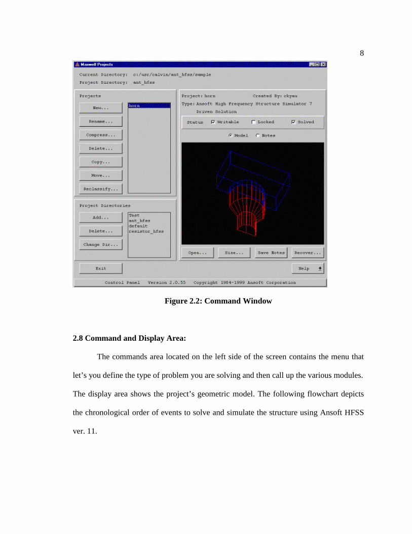
Figure 2.2: Command Window
2.8 Command and Display Area:
The commands area located on the left side of the screen contains the menu that
let’s you define the type of problem you are solving and then call up the various modules.
The display area shows the project’s geometric model. The following flowchart depicts
the chronological order of events to solve and simulate the structure using Ansoft HFSS
ver. 11.
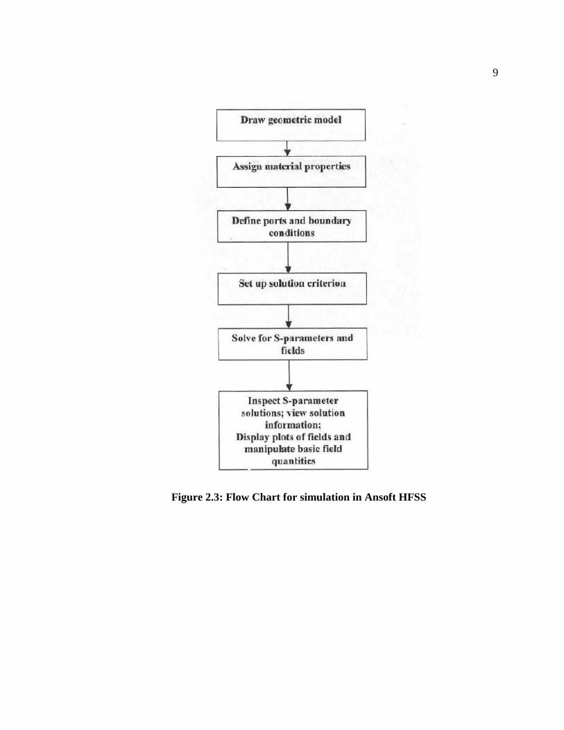
9
Figure 2.3: Flow Chart for simulation in Ansoft HFSS
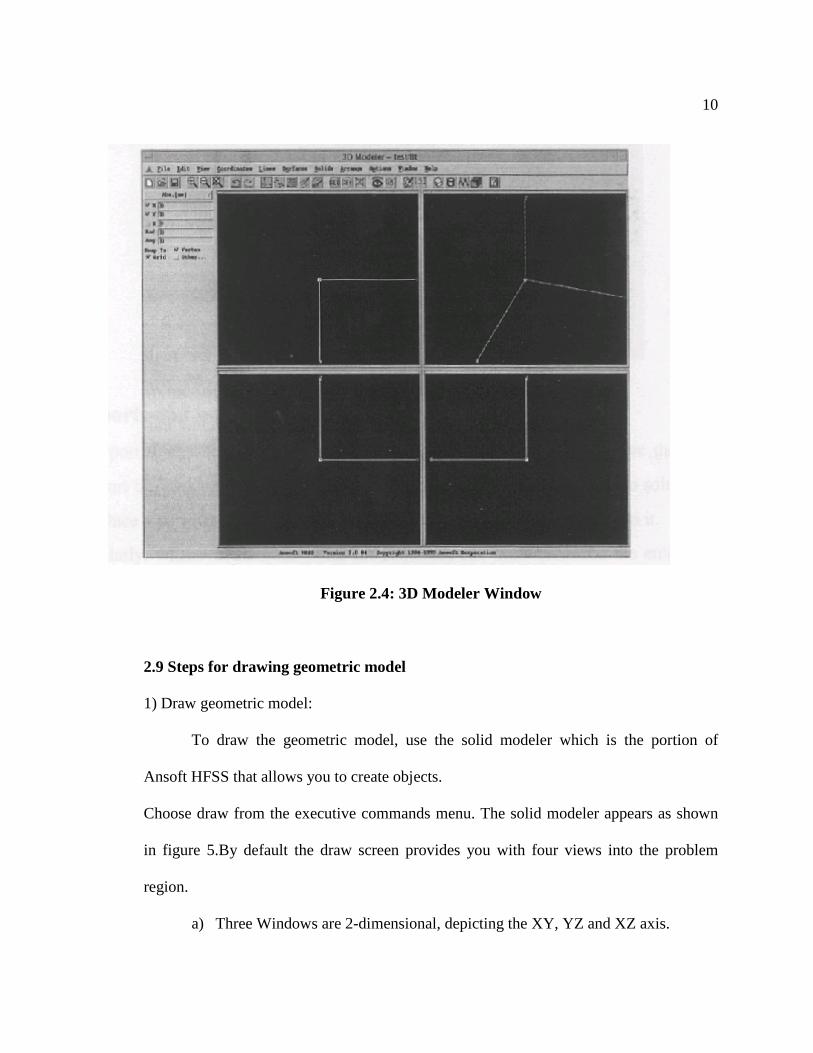
10
Figure 2.4: 3D Modeler Window
2.9 Steps for drawing geometric model
1) Draw geometric model:
To draw the geometric model, use the solid modeler which is the portion of
Ansoft HFSS that allows you to create objects.
Choose draw from the executive commands menu. The solid modeler appears as shown
in figure 5.By default the draw screen provides you with four views into the problem
region.
a) Three Windows are 2-dimensional, depicting the XY, YZ and XZ axis.
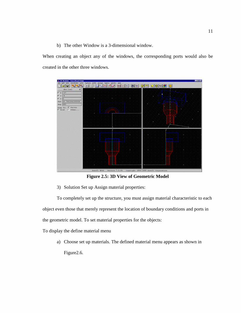
11
b) The other Window is a 3-dimensional window.
When creating an object any of the windows, the corresponding ports would also be
created in the other three windows.
Figure 2.5: 3D View of Geometric Model
3) Solution Set up Assign material properties:
To completely set up the structure, you must assign material characteristic to each
object even those that merely represent the location of boundary conditions and ports in
the geometric model. To set material properties for the objects:
To display the define material menu
a) Choose set up materials. The defined material menu appears as shown in
Figure2.6.
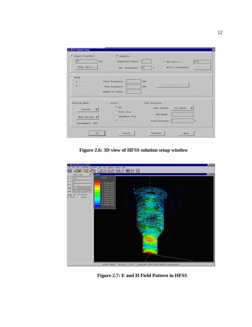
12
Figure 2.6: 3D view of HFSS solution setup window
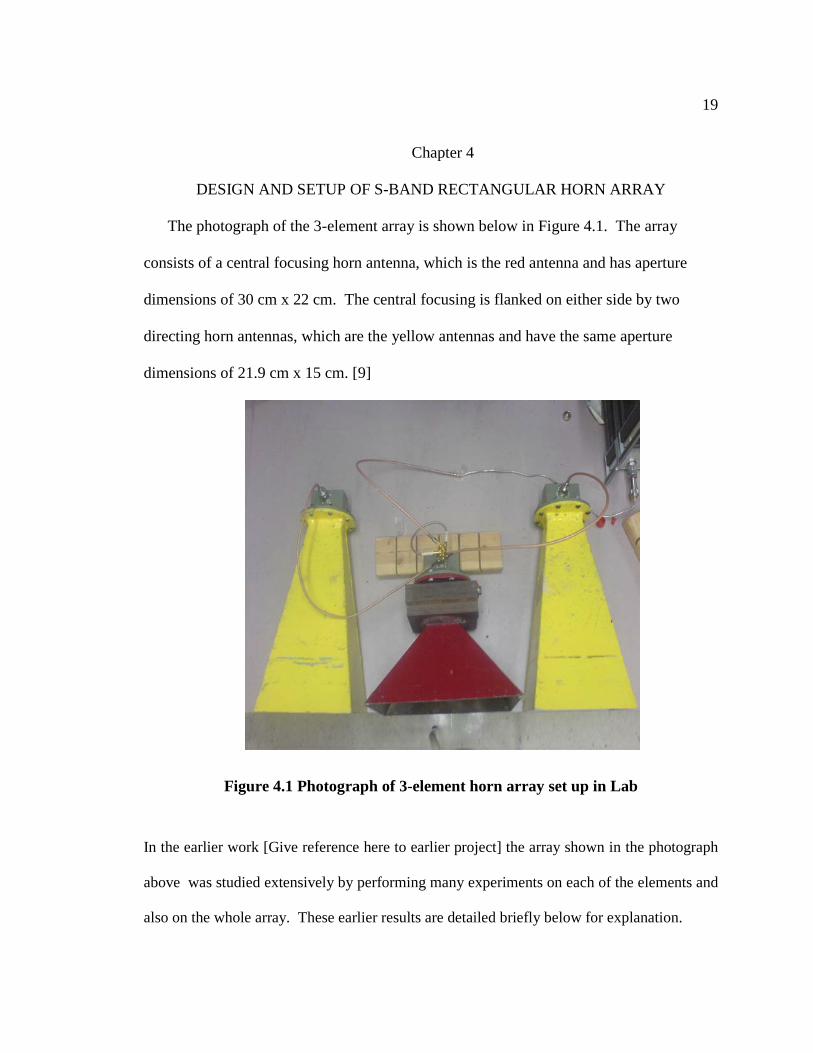
Figure 2.7: E and H Field Pattern in HFSS

13
Figure 2.8: Post progressing far field

14
Chapter 3
INFORMATION ABOUT HYPERTHERMIA
Hyperthermia is overheating of the body. The word is made up of "hyper" (high) and
"thermia" from the Greek word "thermes" (heat). [3]
3.1 Causes of Hyperthermia
Based on these different parameters, Microwave is more dominant in therapeutic
applications in tissue heating. Among all developed methods this is most promising in
the hyperthermia treatment of cancer, and also does not have any side effects and
produces a minimum discomfort for the patient. By generating very narrow beam it is
possible to heat affected tumors of the part of body and protect healthy tissues.
3.2 Meaning of Hyperthermia
Hyperthermia is a heat cancer treatment applied locally to tumors, raising tumor
temperature to about 42.5ºC (108ºF) for about 45 to 60 minutes. Heat improves blood
circulation and makes tumor cells more susceptible to radiation therapy, killing them
more efficiently and quickly. Hyperthermia can be compared with an artificial fever that
attacks cancer cells. The combination of both, hyperthermia and low dose radiation
makes this therapy the most efficient cancer treatment available today. [4]
In local hyperthermia, heat is applied to a small area, such as a tumor, using
various techniques that deliver energy to heat the tumor. Different types of energy may
be used to apply heat, including microwave, radiofrequency, and ultrasound. [6]
In another approach, called perfusion, the patient's blood is removed, heated, and
then pumped into the region that is to be heated internally. Whole-body heating is used to

15
treat metastatic cancer that has spread throughout the body. It can be accomplished using
warm-water blankets, hot wax, inductive coils (like those in electric blankets), or thermal
chambers (like incubators).
A number of challenges must be overcome before hyperthermia can be considered
a standard treatment for cancer. Many clinical trials are being conducted to evaluate the
effectiveness of hyperthermia. Some trials continue to research hyperthermia in
combination with other therapies for the treatment of different cancers. Other studies
focus on improving hyperthermia techniques. [6] Suggests strongly that, when
hyperthermia is used in combination with radiation therapy or chemotherapy, an
improvement in response rates can be achieved. Hyperthermia can be helpful with
palliation, often dramatically reducing pain.
3.3 Methodology for Hyperthermia Treatment [6]
Usually, other forms of cancer therapy such as radiation therapy and
chemotherapy are used in combination with hyperthermia. Hyperthermia increases the
sensitivity of cancer cells towards radiation. It can also harm the cancer cells that are not
affected by radiation. When used in combination with radiation therapy, a gap of one
hour is maintained between the administrations of each treatment. The effects of certain
anti-cancer drugs are also increased through treatment by hyperthermia.
3.4 Types of Hyperthermia
There are 3 types of hyperthermia as described below.
Regional Hyperthermia In this type various approaches are used to heat large areas of
tissue, like cavity, organ or limb.

16
o Deep tissue in this one external applicators is positioned around the body cavity
or organ to be treated, and microwave or radiofrequency energy is focused on the
area to raise its temperature.
o Regional perfusion techniques are used for arms and legs, such as melanoma, or
cancer in some organs, In this one, patient’s blood is removed, heated, and then
refused back into organ. Usually anticancer drugs are given in this treatment.
o Continuous hyperthermic peritoneal perfusion (CHPP) is a technique used to treat
cancers within the peritoneal cavity (the space within the abdomen that contains
the intestines, stomach, and liver), including primary peritoneal mesothelioma and
stomach cancer. During surgery, heated anticancer drugs flow from a warming
device through the peritoneal cavity. The peritoneal cavity temperature reaches
106–108°F.
Local hyperthermia In this type, heat is applied to a small area, such as a tumor, using
various techniques that deliver energy to heat the tumor. Different types of energy may
be used to apply heat, including microwave, radiofrequency, and ultrasound. There are
several approaches to local hyperthermia, depending on the location of tumor. [5]

17
3.5 Types of Hyperthermia Treatment
o External techniques are for tumors which are just below the skin. In this one,
external applicators are positioned around or near the appropriate region, and
energy is focused on the tumor to raise its temperature.
o Intraluminal methods are used to treat tumors within or near body cavities, such
as the esophagus. Probes are placed inside the cavity and inserted into the tumor
to deliver energy and heat that area directly.
o Interstitial techniques are used to treat tumors deep within the body, such as brain
tumors. This technique allows the tumor to be heated to higher temperatures than
external techniques. Under anesthesia, probes or needles are inserted into the
tumor. Imaging techniques, such as ultrasound, may be used to make sure the
probe is properly positioned within the tumor. The heat source is then inserted
into the probe. Radiofrequency ablation is a type of interstitial hyperthermia that
uses radio waves to kill cancer cells.
Whole-body hyperthermia: In this type of hyperthermia cancer that has spread
throughout the body has been treated. This can be done with techniques that increase
the body temperature to 107–108°F, including the use of thermal chambers or hot
water blankets. [6]

18
3.6 Side effects of Hyperthermia
Most normal tissues are not damaged during hyperthermia if the temperature remains
under 111°F. However, due to regional differences in tissue characteristics, higher
temperatures may occur in various spots. This can result in burns, or pain. Perfusion
techniques can cause tissue swelling, blood clots, bleeding, and other damage to the
normal tissues in the perfuse area; however, most of these side effects are for short
period. Whole-body hyperthermia can cause more serious side effects.
3.7 Future scope for Hyperthermia
To be considered for standard treatment, Hyperthermia had few challenges to overcome.
Many clinical trials are being conducted to evaluate the effectiveness of hyperthermia.
Some trials continue to research hyperthermia in combination with other therapies for the
treatment of different cancers. Other studies focus on improving hyperthermia
techniques.
19
Chapter 4
DESIGN AND SETUP OF S-BAND RECTANGULAR HORN ARRAY
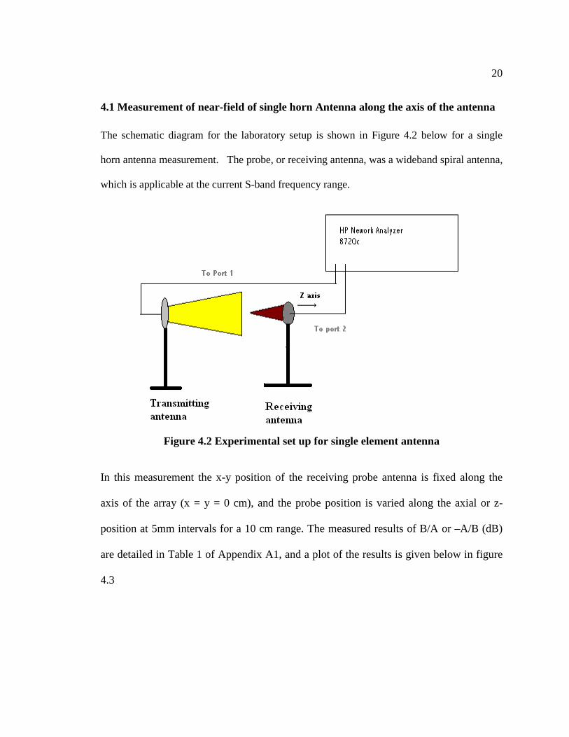
The photograph of the 3-element array is shown below in Figure 4.1. The array
consists of a central focusing horn antenna, which is the red antenna and has aperture
dimensions of 30 cm x 22 cm. The central focusing is flanked on either side by two
directing horn antennas, which are the yellow antennas and have the same aperture
dimensions of 21.9 cm x 15 cm. [9]
Figure 4.1 Photograph of 3-element horn array set up in Lab
In the earlier work [Give reference here to earlier project] the array shown in the photograph
above was studied extensively by performing many experiments on each of the elements and
also on the whole array. These earlier results are detailed briefly below for explanation.
20
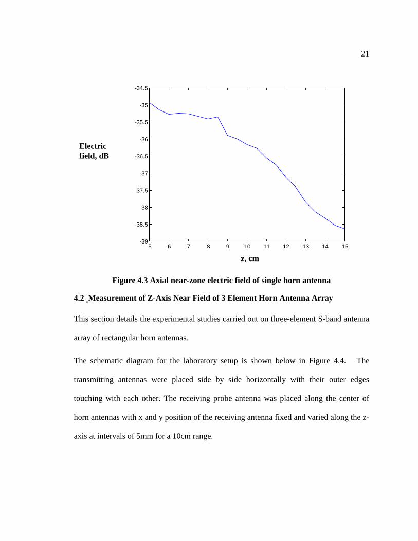
4.1 Measurement of near-field of single horn Antenna along the axis of the antenna
The schematic diagram for the laboratory setup is shown in Figure 4.2 below for a single
horn antenna measurement. The probe, or receiving antenna, was a wideband spiral antenna,
which is applicable at the current S-band frequency range.
Figure 4.2 Experimental set up for single element antenna
In this measurement the x-y position of the receiving probe antenna is fixed along the
axis of the array (x = y = 0 cm), and the probe position is varied along the axial or z-
position at 5mm intervals for a 10 cm range. The measured results of B/A or –A/B (dB)
are detailed in Table 1 of Appendix A1, and a plot of the results is given below in figure
4.3
21
5 6 7 8 9 10 11 12 13 14 15-39
-38.5
-38
-37.5
-37
-36.5
-36
-35.5
-35
-34.5
Figure 4.3 Axial near-zone electric field of single horn antenna
4.2 Measurement of Z-Axis Near Field of 3 Element Horn Antenna Array This section details the experimental studies carried out on three-element S-band antenna
array of rectangular horn antennas.
The schematic diagram for the laboratory setup is shown below in Figure 4.4. The
transmitting antennas were placed side by side horizontally with their outer edges
touching with each other. The receiving probe antenna was placed along the center of
horn antennas with x and y position of the receiving antenna fixed and varied along the z-
axis at intervals of 5mm for a 10cm range.
z, cm
Electric field, dB
22
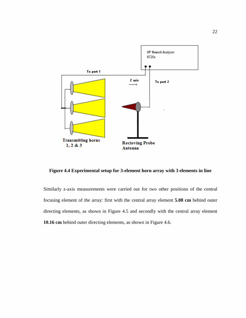
Figure 4.4 Experimental setup for 3-element horn array with 3 elements in line
Similarly z-axis measurements were carried out for two other positions of the central
focusing element of the array: first with the central array element 5.08 cm behind outer
directing elements, as shown in Figure 4.5 and secondly with the central array element
10.16 cm behind outer directing elements, as shown in Figure 4.6.
23
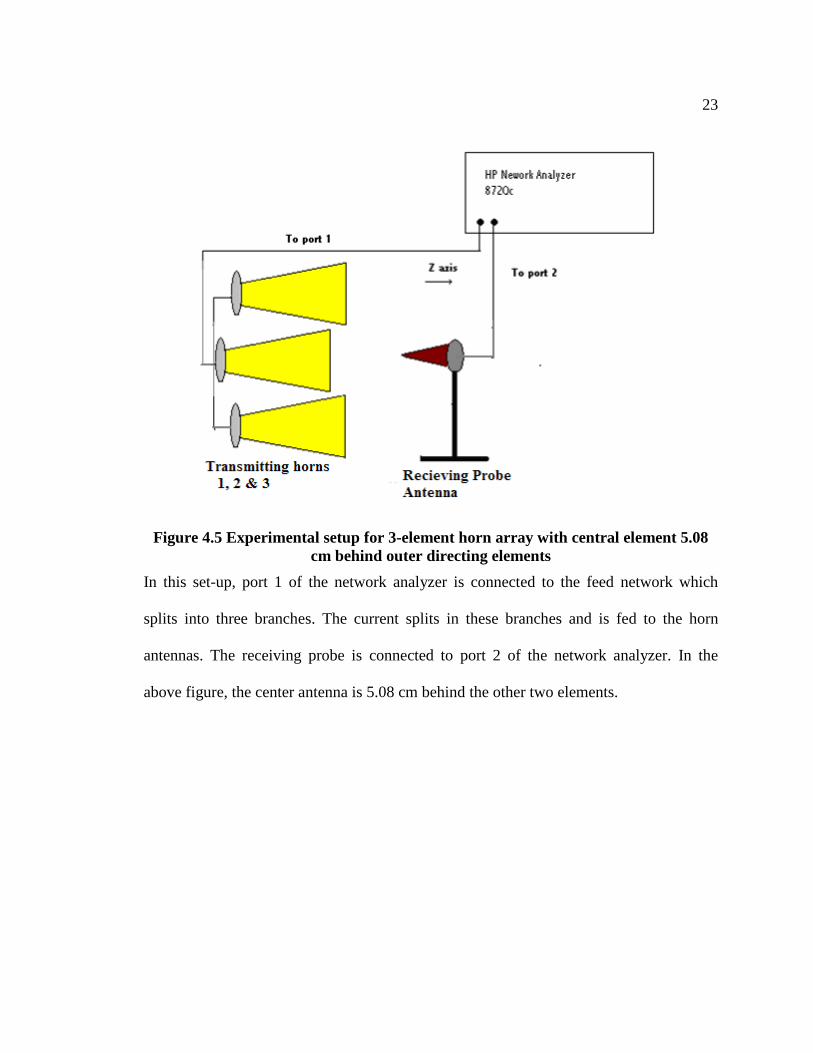
Figure 4.5 Experimental setup for 3-element horn array with central element 5.08 cm behind outer directing elements
In this set-up, port 1 of the network analyzer is connected to the feed network which
splits into three branches. The current splits in these branches and is fed to the horn
antennas. The receiving probe is connected to port 2 of the network analyzer. In the
above figure, the center antenna is 5.08 cm behind the other two elements.
24
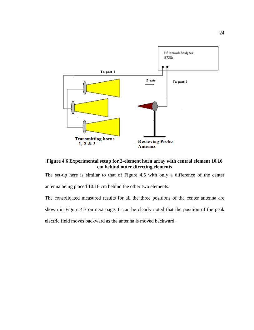
Figure 4.6 Experimental setup for 3-element horn array with central element 10.16 cm behind outer directing elements
The set-up here is similar to that of Figure 4.5 with only a difference of the center
antenna being placed 10.16 cm behind the other two elements.
The consolidated measured results for all the three positions of the center antenna are
shown in Figure 4.7 on next page. It can be clearly noted that the position of the peak
electric field moves backward as the antenna is moved backward.
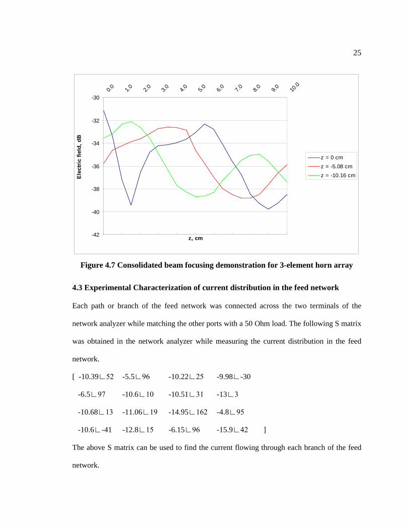
25
-42
-40
-38
-36
-34
-32
-300.0
1.0
2.0
3.0
4.0
5.0
6.0
7.0
8.0
9.0
10
.0
z, cm
Elec
tric
field
, dB
z = 0 cmz = -5.08 cmz = -10.16 cm
Figure 4.7 Consolidated beam focusing demonstration for 3-element horn array
4.3 Experimental Characterization of current distribution in the feed network
Each path or branch of the feed network was connected across the two terminals of the
network analyzer while matching the other ports with a 50 Ohm load. The following S matrix
was obtained in the network analyzer while measuring the current distribution in the feed
network.
[ -10.39∟52 -5.5∟96 -10.22∟25 -9.98∟-30
-6.5∟97 -10.6∟10 -10.51∟31 -13∟3
-10.68∟13 -11.06∟19 -14.95∟162 -4.8∟95
-10.6∟-41 -12.8∟15 -6.15∟96 -15.9∟42 ]
The above S matrix can be used to find the current flowing through each branch of the feed
network.
26
Chapter 5
SIMULATION RESULTS OF S-BAND RECTANGUALR HORN ARRAY
This chapter details the comparison between theoretical and earlier measurement
studies carried out on a three element S-band horn array [9]. All the simulation studies
were done using the Ansoft HFSS, and this was the first project completed in our
laboratory using the new software.
5.1 HFSS setup, simulation and array parameters
The simulation parameters are as follows:
Frequency of simulation: 2.4 GHz
Excitation method: current
Array current distribution: [0.7 1.0 0.7]
Horn antenna material: copper
Simulation environment: air
The schematic, the near field pattern and the electric field distribution as seen in the
HFSS environment is shown below in the following figures. There are three cases
obtained by varying the position of the center element. They were simulated and the
changes in the electric field peak positions were observable.
27
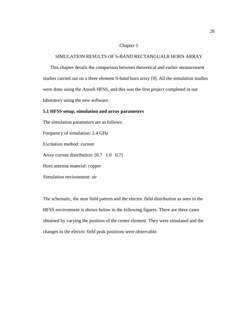
Case 1: In the following three figures, the three array elements are in line
Figure 5.1a HFSS schematic when all elements are in line
The above figure also shows the electric field in V/m along a line of 30 cm centered
along the Z axis. The highest electric field point was noted in this figure and a plane
perpendicular to z axis was placed on that point. The next figure shows us the intensity of
the electric field in the XY plane. The peak was found to be at a distance of
approximately 1 cm from the open end of the horn antenna. So a plane was placed at this
point and the electric field intensity on this plane was generated using HFSS. The
maximum electric field intensity is 561 V/m and the minimum electric field intensity is
27.3 V/m in the plane shown on next page.

28
Figure 5.1b Electric field along a XY plane at the highest field point
Figure 5.1c Near field pattern (Actual distance=30 cm) all horn antennas are in line
29
Figure 5.1c is a rectangular plot of the near field measured along a line of 30 cm. The
maximum electric field is 53.8 dB at a distance of 13.2 cm from the origin.
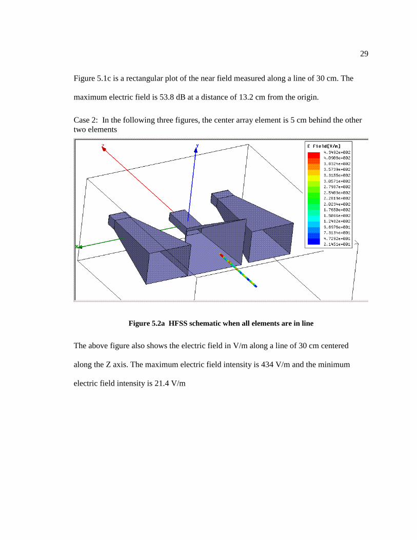
Case 2: In the following three figures, the center array element is 5 cm behind the other two elements
Figure 5.2a HFSS schematic when all elements are in line
The above figure also shows the electric field in V/m along a line of 30 cm centered
along the Z axis. The maximum electric field intensity is 434 V/m and the minimum
electric field intensity is 21.4 V/m

30
Figure 5.2b Electric field along a XY plane at the highest field point The highest electric field point was noted in the previous figure and a plane perpendicular
to z axis was placed on that point. This figure shows us the intensity of the electric field
in the XY plane. The peak was found to be at a distance of approximately 1 cm from the
open end of the horn antenna. So a plane was placed at this point and the electric field
intensity on this plane was generated using HFSS. The maximum field is 475 V/m and
the minimum field is 22.6 V/m.
31
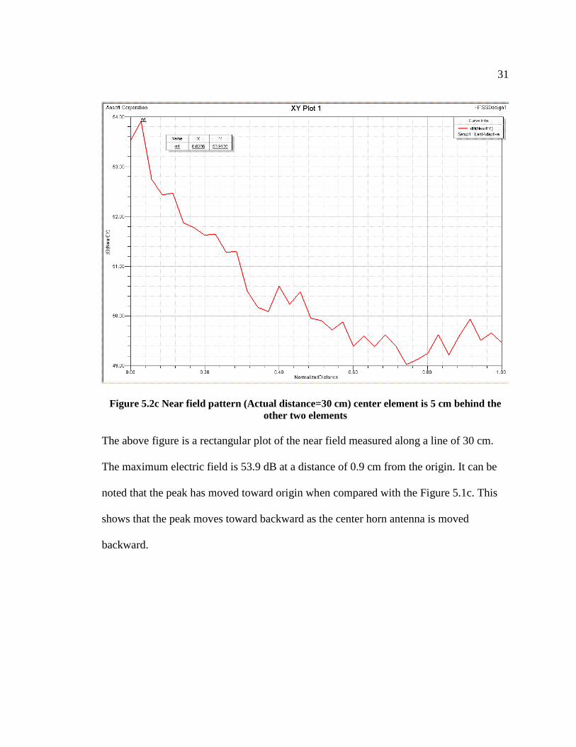
Figure 5.2c Near field pattern (Actual distance=30 cm) center element is 5 cm behind the other two elements
The above figure is a rectangular plot of the near field measured along a line of 30 cm.
The maximum electric field is 53.9 dB at a distance of 0.9 cm from the origin. It can be
noted that the peak has moved toward origin when compared with the Figure 5.1c. This
shows that the peak moves toward backward as the center horn antenna is moved
backward.
32
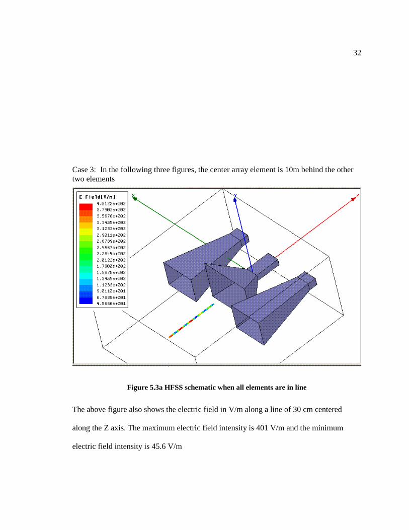
Case 3: In the following three figures, the center array element is 10m behind the other two elements
Figure 5.3a HFSS schematic when all elements are in line
The above figure also shows the electric field in V/m along a line of 30 cm centered
along the Z axis. The maximum electric field intensity is 401 V/m and the minimum
electric field intensity is 45.6 V/m
33
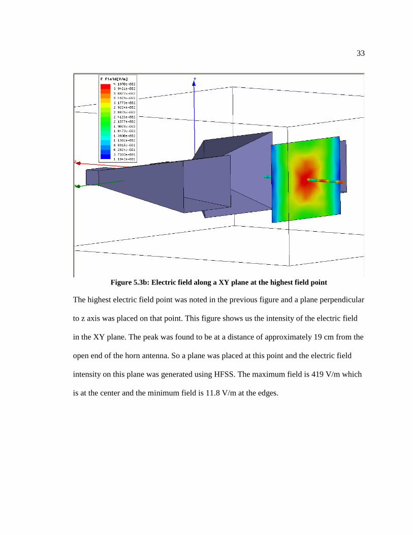
Figure 5.3b: Electric field along a XY plane at the highest field point
The highest electric field point was noted in the previous figure and a plane perpendicular
to z axis was placed on that point. This figure shows us the intensity of the electric field
in the XY plane. The peak was found to be at a distance of approximately 19 cm from the
open end of the horn antenna. So a plane was placed at this point and the electric field
intensity on this plane was generated using HFSS. The maximum field is 419 V/m which
is at the center and the minimum field is 11.8 V/m at the edges.
34
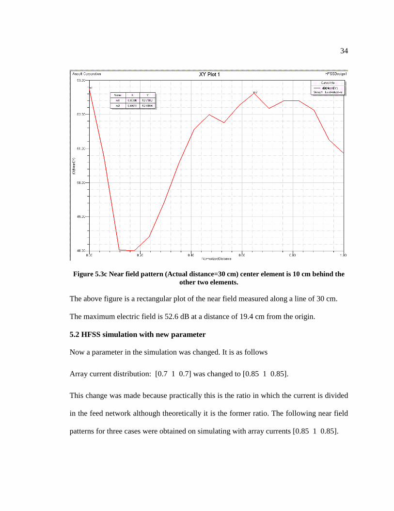
Figure 5.3c Near field pattern (Actual distance=30 cm) center element is 10 cm behind the other two elements.
The above figure is a rectangular plot of the near field measured along a line of 30 cm.
The maximum electric field is 52.6 dB at a distance of 19.4 cm from the origin.
5.2 HFSS simulation with new parameter
Now a parameter in the simulation was changed. It is as follows
Array current distribution: [0.7 1 0.7] was changed to [0.85 1 0.85].
This change was made because practically this is the ratio in which the current is divided
in the feed network although theoretically it is the former ratio. The following near field
patterns for three cases were obtained on simulating with array currents [0.85 1 0.85].
35
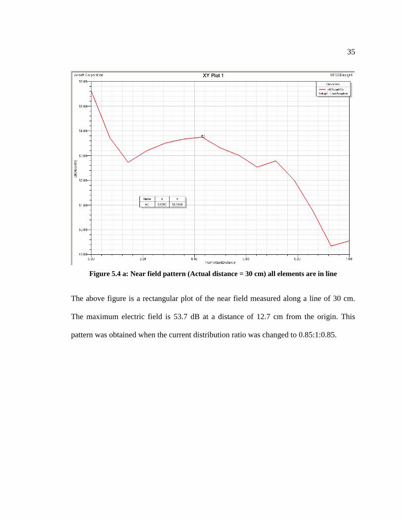
Figure 5.4 a: Near field pattern (Actual distance = 30 cm) all elements are in line
The above figure is a rectangular plot of the near field measured along a line of 30 cm.
The maximum electric field is 53.7 dB at a distance of 12.7 cm from the origin. This
pattern was obtained when the current distribution ratio was changed to 0.85:1:0.85.

36
Figure 5.4b: Near field pattern (Actual distance = 30 cm) center element is 5 cm behind the other two elements
The above figure is a rectangular plot of the near field measured along a line of 30 cm.
The maximum electric field is 53.8 dB at a distance of 0.7 cm from the origin. This
pattern was obtained when the current distribution ratio was changed to 0.85:1:0.85. The
center horn antenna was placed 5 cm behind the other 2 antennas.
37
Figure 5.4c: Near field pattern (Actual distance = 30 cm) center element is 10 cm behind the other two elements
The above figure is a rectangular plot of the near field measured along a line of 30 cm.
The maximum electric field is 53.03 dB at a distance of 19.28 cm from the origin. This
pattern was obtained when the current distribution ratio was changed to 0.85:1:0.85. The
center horn antenna was placed 10 cm behind the other 2 antennas.
It was noted that there was no significant difference in the position of the peak electric
field with the change in array current distribution from [0.7 1 0.7] to [0.85 1 0.85]
38
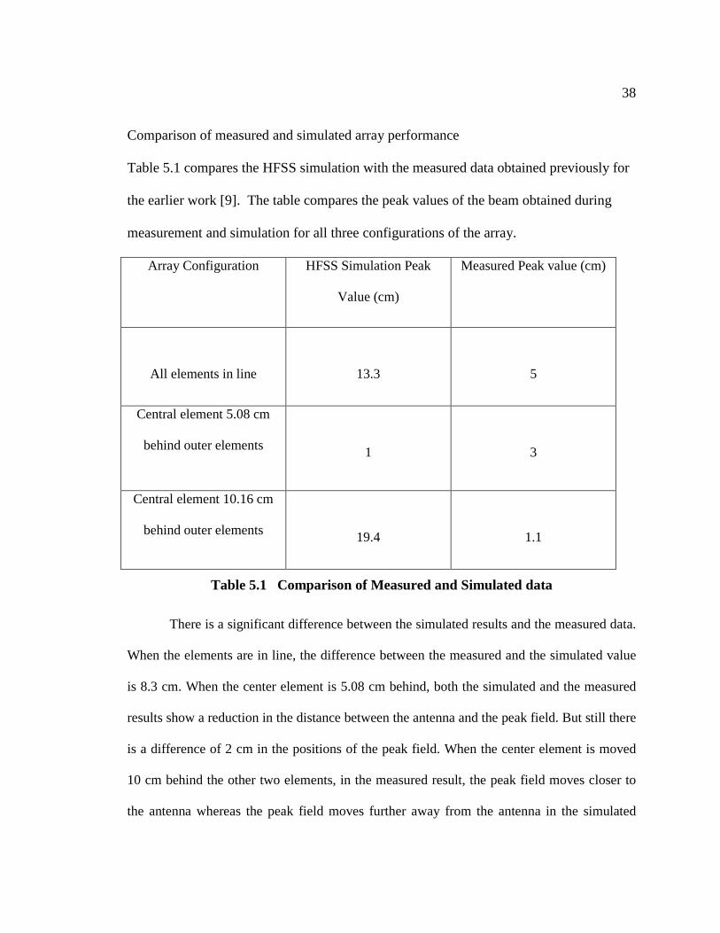
Comparison of measured and simulated array performance
Table 5.1 compares the HFSS simulation with the measured data obtained previously for
the earlier work [9]. The table compares the peak values of the beam obtained during
measurement and simulation for all three configurations of the array.
Array Configuration HFSS Simulation Peak
Value (cm)
Measured Peak value (cm)
All elements in line
13.3
5
Central element 5.08 cm
behind outer elements
1
3
Central element 10.16 cm
behind outer elements
19.4
1.1
Table 5.1 Comparison of Measured and Simulated data
There is a significant difference between the simulated results and the measured data.
When the elements are in line, the difference between the measured and the simulated value
is 8.3 cm. When the center element is 5.08 cm behind, both the simulated and the measured
results show a reduction in the distance between the antenna and the peak field. But still there
is a difference of 2 cm in the positions of the peak field. When the center element is moved
10 cm behind the other two elements, in the measured result, the peak field moves closer to
the antenna whereas the peak field moves further away from the antenna in the simulated

39
result. It is also noted that there were two peaks; one at the line at which the outer elements
are placed (0 cm) and the other peak is at 19.4 cm.
One of the causes for these differences is due to presence of other lab equipments
while measuring data and due to human interference - the person’s proximity to the
transmitting and receiving antennas. Another cause for the difference would be due to the
fact that HFSS computes the results in a adaptive fashion - runs multiple times to find the
accurate solution and it is possible that the number of adaptive solutions chosen to compute
these results are not sufficient. Yet another cause would be loose connections between the
connectors of the network analyzer while measuring data.

40
Chapter 6
CONCLUSION AND SCOPE FOR FUTURE WORK
This project was aimed at the accurate simulation of the near-field effects of a 3-
element rectangular horn array antenna operating in the S-band frequency range of 2.45
GHz. This frequency has applications in medical field such as microwave hyperthermia,
where focused microwave radiation is used to treat tumors. In an earlier project, the array
was designed, assembled and its near-field performance was measured on the HP 8720C
Network Analyzer in the CSUS Microwave Laboratory. Currently, the simulation effort
is to model the array performance by using the HFSS software, and to match the earlier
measured results.
The simulation results differed slightly from the measured results but showed that
clear beam formation is obtained in the near-field of the array. Additionally, the results
also exhibited the beam control of the array, with the beam being capable of being
adjusted over a 5 cm axial range. Two-dimensional planar measurements and simulation
studies were also conducted to validate the volumetric focusing properties of the array.
The latter results also showed clear beam focusing in the planar x-y plane of the array.
Future work will focus on improving the efficiency of the array, with an aim to
increase the resolution of the beam so that much clearer focus can be obtained for
hyperthermia applications. This would involve trying out different current distributions
for the array elements, which can be achieved by the use of attenuators in the feed section
of the array.
41
REFERENCES
[1] E.L. Jones, J.R. Oleson, L.R. Prosnitz, T.V. Samulski, Z. Vujaskovic, D.Yu, L.L. Sanders, and M.W. Dewhirst, “Randomized trial of hyperthermia and radiation for superficial tumors”, J Clin. Oncol. 2005 May 1;23(13):3079-85.
[2] Manual of ANSOFT HFSS ver 11.0, ANSOFT, 2007
[3] “Hyperthermia and heat related illness: Question – Answers” retrieved from http://www.medicinenet.com/hyperthermia/article.htm#1 on Nov 2 2009.
[4] “Valley Center Institute: Information” retrieved from: http://www.vci.org on Oct.28 2009
[5] Maluta S, Dall'Oglio S, Romano M, Marciai N, Pioli F, Giri MG, Benecchi PL, Comunale L, Porcaro AB., “Conformal radiotherapy plus local hyperthermia in patients affected by locally advanced high risk prostate cancer: preliminary results of
a prospective phase II study”, Int J Hyperthermia. 2007 Aug; 23(5):451-6.
[6] “Hyperthermia in Cancer Treatment: Questions and Answers” retrieved from: http://www.cancer.gov/cancertopics/factsheet/Therapy/hyperthermia, on Nov. 3 2009
[7] “Hyperthermia centers: Information” retrieved from: http://www.geocities.com/HotSprings/Villa/5443/alts/hytherm.html, on Nov 8 2009
[8] David M Pozar “Microwave Engineering” Third edition, Wiley Publication, Year 2003
[9] Sridhar Nayakwadi, Lakshmi B.T.V, “Near-Field Beam Forming for Medical applications using S-band rectangular horn antenna array”. Master of Science Project, Department of Electrical and Electronics Engineering, August 2008.
Top Related
Copyright © 2022 FDOKUMEN

