


Bahasa
Halaman
Hukum


BioOne sees sustainable scholarly publishing as an inherently collaborative enterprise connecting authors, nonprofit publishers, academic institutions, researchlibraries, and research funders in the common goal of maximizing access to critical research.
Space use by giant otter groups in the Brazilian PantanalAuthor(s): Caroline Leuchtenberger, Luiz Gustavo Rodrigues Oliveira-Santos, William Magnusson, andGuilherme MourãoSource: Journal of Mammalogy, 94(2):320-330.Published By: American Society of MammalogistsDOI: http://dx.doi.org/10.1644/12-MAMM-A-210.1URL: http://www.bioone.org/doi/full/10.1644/12-MAMM-A-210.1
BioOne (www.bioone.org) is a nonprofit, online aggregation of core research in the biological, ecological, andenvironmental sciences. BioOne provides a sustainable online platform for over 170 journals and books publishedby nonprofit societies, associations, museums, institutions, and presses.
Your use of this PDF, the BioOne Web site, and all posted and associated content indicates your acceptance ofBioOne’s Terms of Use, available at www.bioone.org/page/terms_of_use.
Usage of BioOne content is strictly limited to personal, educational, and non-commercial use. Commercial inquiriesor rights and permissions requests should be directed to the individual publisher as copyright holder.

Journal of Mammalogy, 94(2):320–330, 2013
Space use by giant otter groups in the Brazilian Pantanal
CAROLINE LEUCHTENBERGER,* LUIZ GUSTAVO RODRIGUES OLIVEIRA-SANTOS, WILLIAM MAGNUSSON, AND
GUILHERME MOURAO
Laboratory of Wildlife, Embrapa Pantanal, Rua 21 de Setembro, 1880, CEP 79320-900, Corumba, MS, Brazil (CL andGM)Department of Ecology, Universidade Federal do Rio de Janeiro, Av. Carlos Chagas Filho, 373–Sala A027, CEP 68020–Ilha do Fundao, CEP 21941-902, Rio de Janeiro, RJ, Brazil (LGROS)Graduate Program in Ecology, Instituto Nacional de Pesquisas da Amazonia (INPA), Av. Andre Araujo, 2936, CEP69083-000, Manaus, AM, Brazil (CL and WM)
* Correspondent: [email protected]
Giant otters (Pteronura brasiliensis) live in groups that seem to abandon their territories during the flooding
season. We studied the spatial ecology of giant otter groups during dry and wet seasons in the Vermelho and
Miranda rivers in the Brazilian Pantanal. We monitored visually or by radiotelemetry 10 giant otter groups
monthly from June 2009 to June 2011.We estimated home-range size for all groups with the following methods:
linear river length, considering the extreme locations of each group, and fixed kernel. For the radiotracked
groups, we also used the k-LoCoh method. Spatial fidelity and habitat selection of giant otter groups were
analyzed seasonally. On the basis of k-LoCoh (98%) method, home-range sizes during the wet season (3.6–7.9
km2) were 4 to 59 times larger than during the dry season (0.1–2.3 km2). Home-range fidelity between seasons
varied among giant otter groups from 0% to 87%, and 2 radiotagged groups shifted to flooded areas during the
wet seasons. Giant otter groups were selective in relation to the composition of the landscape available during the
dry seasons, when the river was used more intensively than other landscape features. However, they seemed to
be less selective in positioning activity ranges during the wet season. During this season, giant otters were
frequently observed fishing in the areas adjacent to the river, such as flooded forest, grassland, and swamps.
Key words: habitat selection, home range, landscape selection, Pteronura brasiliensis, site fidelity
� 2013 American Society of Mammalogists
DOI: 10.1644/12-MAMM-A-210.1
Animals adopt different strategies to deal with spatial and
temporal heterogeneity of environmental features. Most species
constrain their activities to an area on the landscape defined as
a home range, which comprises areas used in diverse ways for
survival, reproduction, and other activities that maximize
fitness (Krebs and Davies 1997; Powell 2000). Some core areas
are used more intensely within the boundaries of the home
range and commonly contain refuges and more defendable
food sources (Kernohan et al. 2001; Samuel et al. 1985). The
maintenance of the home range in space and time is favored by
a cognitive map (Spencer 2012) that provides site familiarity,
which enhances the owners’ fitness, increasing their ability to
forage and to move rapidly and safely in the area (Stamps
1995).
Some landscape features are used more by a species than
their proportional availability in the environment (Aebischer et
al. 1993; Johnson 1980). However, under highly seasonal
fluctuations, changes in habitat and resource availability may
induce a shift in the animal’s spatial organization and habitat
use through different seasons (Arthur et al. 1996; Humphrey
and Zinn 1982). Availability and abundance of food resources,
together with the metabolic needs of each species, seem to be
the most important variables determining the home range size
and habitat selection of carnivores (e.g., Dillon and Kelly 2008;
Macdonald 1983; Valenzuela and Ceballos 2000). Space use
by semiaquatic mammals is strongly affected by the availabil-
ity of water bodies and prey, and such relationships have been
reported for several species of otters (Blundell et al. 2000;
Garcia de Leaniz et al. 2006; Kruuk 2006; Melquist and
Hornocker 1983). In places with well-defined hydrological
cycles, flooding increases the amount of water in the landscape
and may result in the dispersal of fish assemblages across vast
w w w . m a m m a l o g y . o r g
320

flooded areas (Wantzen et al. 2002; Winemiller and Jepsen
1998), which may attract fish predators and induce predictable
movement patterns of the piscivores.
Giant otters (Pteronura brasiliensis) feed mainly on fish, and
information on their spatial ecology is limited to direct
observations during the dry season, when groups maintain
linear territories along water bodies (Duplaix 1980; Evangelista
and Rosas 2011a; Laidler 1984; Leuchtenberger and Mourao
2008; Ribas 2004; Schweizer 1992; Tomas et al. 2000; Utreras
et al. 2005). Groups build dens and campsites with communal
latrines throughout their home ranges that are used for resting,
scent-marking, and rearing cubs (Duplaix 1980; Leuchten-
berger and Mourao 2009; Lima et al. 2012). During the rainy
season, giant otters seem to relinquish their territories to follow
spawning fish into the flooded forest and swamps, and to
search for emergent sites for building dens and campsites
(Duplaix 1980). Seasonal shifts in movement patterns can
increase home-range sizes of giant otter groups, which have
been estimated to be 4 to 13 times larger during the rainy
season (Utreras et al. 2005). However, in the absence of
fluctuating water levels, giant otter groups seem to maintain
their territories throughout the year (Laidler 1984).
The Pantanal is an extensive wetland located near the center
of South America and it is subject to a strong annual flood
pulse, which is considered to be the most important ecological
phenomenon for the maintenance of local biodiversity (Alho
2008). Giant otters are locally abundant and distributed
throughout this region (Leuchtenberger and Mourao 2008;
Tomas et al. 2000). In this paper, we examine home-range size,
home-range fidelity, and habitat selection of giant otters in the
Brazilian Pantanal on the basis of direct observations and
radiotelemetry, with the aim of answering the following
questions: Is home-range size during the wet season larger
than in the dry season? Do giant otter groups show home-range
fidelity within and between seasons? Do habitat-selection
patterns differ between seasons?
MATERIAL AND METHODS
From June 2009 to June 2011, we monitored 10 giant otter
groups in the Vermelho River (198340S; 578010W) and a stretch
of the Miranda River (198360S, 578000W), totaling 119 linear
km of river, in the southern Pantanal of Brazil. The annual
precipitation in the region is about 1,200 mm, with most of the
rain falling between November and March (Hamilton et al.
1996). Due to the low declivity and seasonal inundation,
almost 80% of the plain undergoes transition from terrestrial to
aquatic habitat during the rainy season (Alho 2008). We
measured the level of the Miranda River every day at a fixed
station (198340S, 578010W), and it varied from 126 to 481 cm
during the study period. Flooding tended to be abrupt, and the
transition from wet to dry occurred within a few weeks. On the
basis of the river-level measurements, we recognized 2 dry
seasons (June–December 2009 and July 2010–January 2011)
and 2 wet seasons (January–June 2010 and February–June
2011) during the study.
We monitored giant otter groups by boat, using a video
camera (Canon HF-200, Lake Success, New York) to record
individual natural marks on the throat of otters and their
behaviors. This allowed us to identify the sex, position in the
group hierarchy, group composition, and other details about the
individuals. The location of individuals, groups, dens, latrines,
and other vestiges were registered by a global positioning
system (GPS) receptor (Garmin Etrex, Inc., Olathe, Kansas).
Between November 2009 and July 2010, we undertook three
10-day field trips to capture and implant radiotransmitters in
individuals from different groups of giant otters. In each
campaign, we first searched for active dens suitable for setting
traps (i.e., dens with 1 or few entrances relatively free of
entanglements of roots and vegetation). We blocked the den
entrance with a funnel-shaped net late at night, as described by
Silveira et al. (2011), and waited in the vicinity of the den to
capture the individuals in the early morning. We captured 2
dominant males (from groups G2 and G12) and 1 adult
subordinate male (group G10). The mean weight of captured
individuals was 30.97 kg (SD¼ 1.75) and the mean total body
length 178 cm (SD ¼ 6.25).
We chemically immobilized the animals after capture using
a dosage of 2.0 mg/kg of a combination of tiletamine and
zolazepam (Zoletil, Virbac, Carros-Cedex, France) and applied
a complementary dosage of 1.5 mg/kg ketamine hydrochloride
10% (Vetaset, Fort Dodge, Campinas, Brazil) combined with
0.25 mg/kg midazolam (Dormonid, Roche, Jaguare, Brazil).
Radios were implanted intraperitoneally by a registered
veterinarian. During surgery, we applied 0.5 ml of intramus-
cular penicillin (Pentabiotico Veterinario, Fort Dodge Animal
Health, Campinas, Brazil) and a subcutaneous dosage of 2 mg/
kg of anti-inflammatory/analgesic (Ketoprofen 1%, Merial
Animal Health, Paulınea, Brazil). We examined each captured
individual for general body condition, photographed their
throat markings, and took body measurements. The radio-
transmitter (M1245B, Advanced Telemetry System, Isanti,
Minnesota) weighed 42 g (~0.1% of body weight). All
handling and surgical procedures followed the guidelines of the
American Society of Mammalogists for the use of wild
mammals in research (Sikes et al. 2011), and were authorized
under license No. 12794/4 of the Brazilian Institute of
Environment and Renewable Natural Resources. We released
the radiotagged giant otters, after they recovered from the
anesthesia, at the place of capture or near their group.
We radiotracked animals by boat or walking on the bank
with a Yagi antenna (RA-17, Telonics, Mesa, Arizona)
attached to a 2.5-m pole and connected to a TR4-receiver
(Telonics). One group (G2) was monitored from November
2009 to June 2010, and 2 groups (G10 and G12) from July
2010 to June 2011, totaling 153 days of monitoring. Radio-
tagged animals were monitored from 0500 h, when almost all
members of the group had left the den, to 1900 h or when the
whole group had entered the den, during 8–10 consecutive
days every month. On 2 occasions, when the tagged animals
were not found for 2 consecutive months, we undertook aerial
surveys with a fixed-wing aircraft (CESSNA-182) to locate
April 2013 321LEUCHTENBERGER ET AL.—SPACE USE OF GIANT OTTERS

them. Once located from the ground, we followed the animals
as silently as possible, keeping a distance that apparently did
not disturb their behavior. We recorded locations with the GPS
every 30 min when the group could be seen until we lost the
radio signal. Since groups G10 and G12 had territories near
each other, we monitored these groups in alternate periods
(0500–1200 h or 1230–1900 h). We undertook nocturnal
monitoring irregularly, but these data were not considered for
home-range and habitat-use analyses, as movements were very
limited at night. We used only locations recorded more than 10
days after capture in the analyses to avoid abnormal behavior
due to the effects of capture and handling.
Home range.—Removal of sequential data to increase
independence of locations can reduce the biological meaning
of the information (Blundell et al. 2001; De Solla et al. 1999;
Reynolds and Laundre 1990; Rooney et al. 1998). Also, giant
otters cover much of their home range every day, so
observations taken over 6–13 h per day tend not to be
clustered in a limited part of the home range. Therefore, we
considered all sequential locations (n ¼ 2,321) acquired by
radiotelemetry for home-range analysis, as well as some visual
locations of the group G2 (n ¼ 38) made before the capture
event.
To allow comparison with other studies, we estimated home
range for all groups as linear river length (RL) within the
extreme locations of each group, which is commonly used to
estimate giant otter linear home range (Evangelista and Rosas
2011a), and the fixed-kernel estimator with ad hoc estimation
of the h value. For the radiotracked groups, for which we
obtained more locations, we also used the k-LoCoh method
(Getz and Wilmers 2004). Because groups sometimes shifted
their areas from one season to another (Leuchtenberger and
Mourao 2008), we stratified the home-range estimates by
seasons in cases where we had more than 20 locations for a
given group in a given season. All home-range analyses were
undertaken in the R software (R Development Core Team
2011), using the packages ade4 (Thioulouse et al. 1997),
adehabitat and adehabitatHR (Callenge 2006), gpclib, maptools
(Lewin-Koh et al. 2009), rgdal (Keitt et al. 2010), rgeos
(Renard and Bez 2005), and shapefiles (Stabler 2003). We
calculated 98% and 95% isopleths for k-LoCoh analyses and
95% isopleths for the kernel estimator of total home-range size
and the 50% isopleths to delimit core areas.
We measured the linear extension of river (RL) and/or other
water bodies, such as ponds, streams, or flooded areas along
roads, within the extreme locations of each monitored group
using the GPS TrackMaker software (Ferreira 2004). For the
kernel analysis, we tried to use the least-square cross-validation
method, but this analysis did not converge. Therefore, we
chose the h-value of h¼ 80 and h¼ 100, respectively, for the
dry and wet seasons analyses of all groups, as they resulted in
kernel-contour shapes that visually better accommodated the
group locations.
To evaluate if we had enough locations to determine the
home-range areas of radiotracked giant otter groups, we plotted
the cumulative estimated LoCoh 100% areas chronologically.
For this analysis, we fixed the number of nearest-neighbor
locations (k) to 5. However, to estimate the appropriate k for
calculation of the group’s home-range area, we followed the
procedure described in Ryan et al. (2006). That is, we plotted
the home-range areas on the basis of 100% of locations,
calculated with k values varying from 2 to 30 (100% isopleths)
for each group. The asymptote of the 3 radiotagged groups was
estimated to be approximated at k ¼ 16, which was the value
used for the k-LoCoh analyses.
We overlapped the home ranges and core areas (estimated
with the kernel and LoCoh methods) of groups that were
monitored in consecutive seasons to estimate the percentage of
area fidelity. These were estimated with ArcMap 10.0 software
(ESRI 2010), using the clip function. We also calculated the
daily speed of each radiotracked group by season, dividing the
daily mean of the Euclidean distance traveled among
consecutive locations by the respective mean of time interval.
Selection of landscape features.—Here we use habitat to
mean a category of physical environment that occurs in a
circumscribed area that is available to an organism or group of
organisms. In this sense, habitats include areas that may never
be used by the organism under study. Used in this way, habitats
are not necessarily related to particular organisms, and do not
exist as inherent natural objects in the landscape, but are
merely convenient categories that humans use to get a
preliminary understanding of the spatial relationships of
organisms to their environment. We created 3 landscape-
category maps, representing 3 seasons (dry, wet 2010, and wet
2011), due to the differences in the flood levels of the wet
seasons during the study period. We classified Landsat TM5
(NASA Landsat Program 2009, 2010, 2011) satellite images
within seasons using the Kmedia method in the Spring v.4.3.3
software (Camara et al. 1996). We digitalized an image taken
during the dry season of 2009 in Google Earth and classified it
in ArcMap 10.0 software (ESRI 2010). The wet-season images
were overlapped on this dry-season image, recovering some
landscape-unit types that could not be classified automatically.
We used 6 landscape-unit categories: river; pond (comprising
permanent and temporary freshwater ponds, and artificial
ponds created during the construction of roads or water
reservoirs used for cattle); swamp (water bodies that act as a
transition between the aquatic and terrestrial, normally found at
the edge of ponds, streams, and rivers, and that are dominated
by grasses sometimes including isolated trees and shrubs);
seasonally flooded grassland (seasonally flooded plains,
including the grasslands); forest (riparian forest,
semideciduous forest, and/or woodland savanna); and
grassland (nonflooded matrix of grasses and herbs, we also
included in this class roads and a few riparian human
communities that were established in areas that originally had
this vegetation cover).
We analyzed landscape-category selection of giant otter
groups using a log-ratio compositional analysis (Aebisher et al.
1993) with 2,000 permutations in the R 2.13 software, using
the packages adehabitat (Callenge 2006), maptools (Lewin-
Koh et al. 2009), raster (Hijmans and van Etten 2010), rgdal
322 Vol. 94, No. 2JOURNAL OF MAMMALOGY
(Keitt et al. 2010), rgeos (Renard and Bez 2005), and shapefiles
(Stabler 2003). We undertook landscape-category selection
analysis for 8 groups (G1–G4, G8–G12) within the 2nd and
3rd levels proposed by Johnson (1980), which are the home-
range area selected by each group in the study area, and space
use (locations) of the groups within their home ranges. A buffer
of 2 km was incorporated around each location of giant otters
during the monitoring period in the study area (Blundell et al.
2001) using ArcMap 10.0 software. This buffer range was
considered the study area for compositional analysis within
home ranges. For home-range availability, we used the fixed-
kernel contours with ad hoc estimation of the h values. We
undertook eigen analysis of selection ratio as described by
Callenge and Dufour (2006), which assigns scores to each
giant otter group and habitat, resulting in a measure of habitat
selection for each group. We counted the number of dens and
campsites built by giant otter groups in each landscape feature
to analyze the proportion of refuge and site locations in each
habitat.
RESULTS
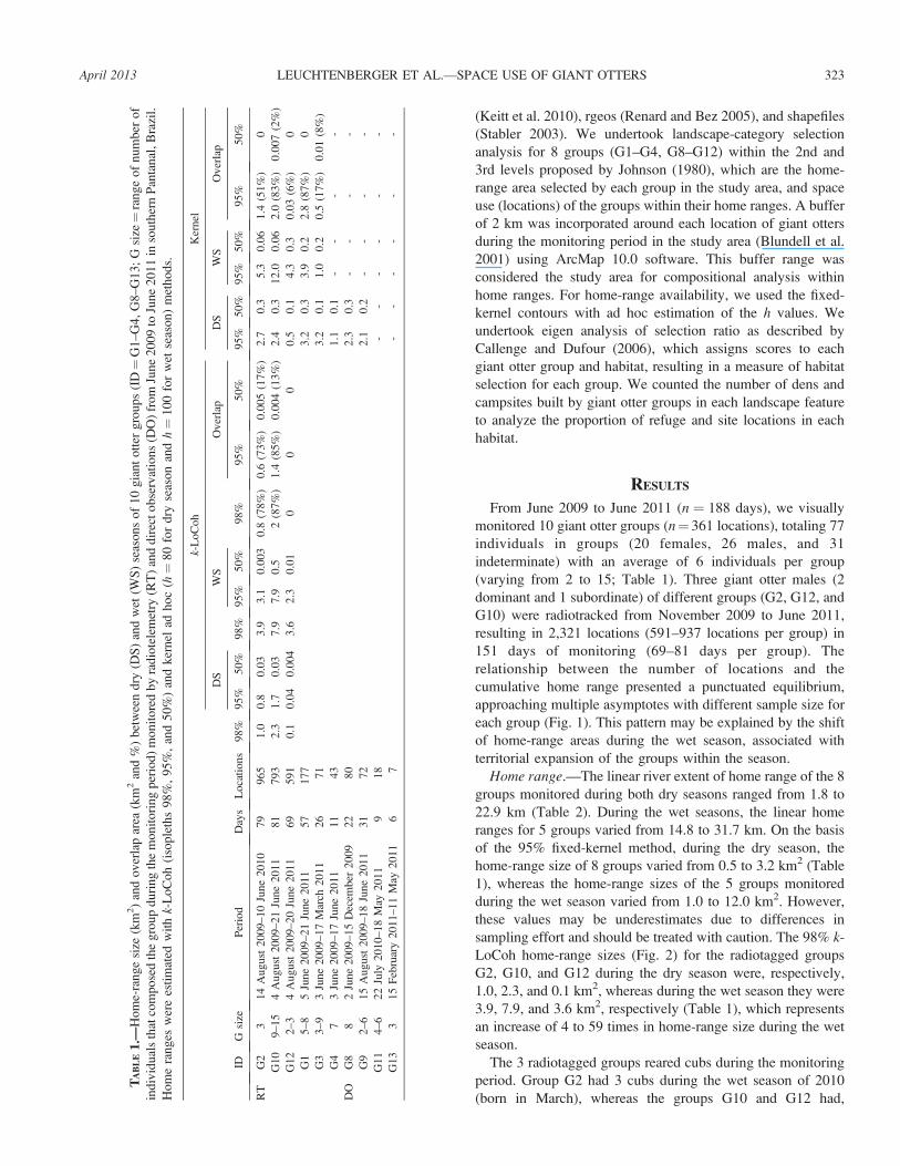
From June 2009 to June 2011 (n ¼ 188 days), we visually
monitored 10 giant otter groups (n¼ 361 locations), totaling 77
individuals in groups (20 females, 26 males, and 31
indeterminate) with an average of 6 individuals per group
(varying from 2 to 15; Table 1). Three giant otter males (2
dominant and 1 subordinate) of different groups (G2, G12, and
G10) were radiotracked from November 2009 to June 2011,
resulting in 2,321 locations (591–937 locations per group) in
151 days of monitoring (69–81 days per group). The
relationship between the number of locations and the
cumulative home range presented a punctuated equilibrium,
approaching multiple asymptotes with different sample size for
each group (Fig. 1). This pattern may be explained by the shift
of home-range areas during the wet season, associated with
territorial expansion of the groups within the season.
Home range.—The linear river extent of home range of the 8
groups monitored during both dry seasons ranged from 1.8 to
22.9 km (Table 2). During the wet seasons, the linear home
ranges for 5 groups varied from 14.8 to 31.7 km. On the basis
of the 95% fixed-kernel method, during the dry season, the
home-range size of 8 groups varied from 0.5 to 3.2 km2 (Table
1), whereas the home-range sizes of the 5 groups monitored
during the wet season varied from 1.0 to 12.0 km2. However,
these values may be underestimates due to differences in
sampling effort and should be treated with caution. The 98% k-
LoCoh home-range sizes (Fig. 2) for the radiotagged groups
G2, G10, and G12 during the dry season were, respectively,
1.0, 2.3, and 0.1 km2, whereas during the wet season they were
3.9, 7.9, and 3.6 km2, respectively (Table 1), which represents
an increase of 4 to 59 times in home-range size during the wet
season.
The 3 radiotagged groups reared cubs during the monitoring
period. Group G2 had 3 cubs during the wet season of 2010
(born in March), whereas the groups G10 and G12 had,
TA
BL
E1
.—H
om
e-ra
ng
esi
ze(k
m2)
and
ov
erla
par
ea(k
m2
and
%)
bet
wee
nd
ry(D
S)
and
wet
(WS
)se
aso
ns
of
10
gia
nt
ott
erg
rou
ps
(ID¼
G1
–G
4,
G8
–G
13
;G
size¼
ran
ge
of
nu
mb
ero
f
ind
ivid
ual
sth
atco
mp
ose
dth
eg
rou
pd
uri
ng
the
mo
nit
ori
ng
per
iod
)m
on
ito
red
by
rad
iote
lem
etry
(RT
)an
dd
irec
to
bse
rvat
ion
s(D
O)
fro
mJu
ne
20
09
toJu
ne
20
11
inso
uth
ern
Pan
tan
al,B
razi
l.
Ho
me
ran
ges
wer
ees
tim
ated
wit
hk-
Lo
Co
h(i
sop
leth
s9
8%
,9
5%
,an
d5
0%
)an
dk
ern
elad
ho
c(h¼
80
for
dry
seas
on
and
h¼
10
0fo
rw
etse
aso
n)
met
ho
ds.
IDG
size
Per
iod
Day
sL
oca
tio
ns
98
%
k-L
oC
oh
Ker
nel
DS
98
%
WS
98
%
Ov
erla
pD
SW
SO
ver
lap
95
%5
0%
95
%5
0%
95
%5
0%
95
%5
0%
95
%5
0%
95
%5
0%
RT
G2
31
4A
ug
ust
20
09–
10
Jun
e2
01
07
99
65
1.0
0.8
0.0
33
.93
.10
.003
0.8
(78
%)
0.6
(73
%)
0.0
05
(17
%)
2.7
0.3
5.3
0.0
61
.4(5
1%
)0
G1
09
–1
54
Au
gu
st2
00
9–
21
Jun
e2
01
18
17
93
2.3
1.7
0.0
37
.97
.90
.52
(87
%)
1.4
(85
%)
0.0
04
(13
%)
2.4
0.3
12
.00
.06
2.0
(83
%)
0.0
07
(2%
)
G1
22
–3
4A
ug
ust
20
09–
20
Jun
e2
01
16
95
91
0.1
0.0
40
.004
3.6
2.3
0.0
10
00
0.5
0.1
4.3
0.3
0.0
3(6
%)
0
G1
5–
85
Jun
e2
00
9–
21
Jun
e2
01
15
71
77
3.2
0.3
3.9
0.2
2.8
(87
%)
0
G3
3–
93
Jun
e2
00
9–
17
Mar
ch2
01
12
67
13
.20
.11
.00
.20
.5(1
7%
)0
.01
(8%
)
G4
73
Jun
e2
00
9–
17
Jun
e2
01
11
14
31
.10
.1-
--
-
DO
G8
82
Jun
e2
00
9–
15
Dec
emb
er2
00
92
28
02
.30
.3-
--
-
G9
2–
61
5A
ug
ust
20
09–
18
Jun
e2
01
13
17
22
.10
.2-
--
-
G1
14
–6
22
July
20
10–
18
May
20
11
91
8-
--
--
-
G1
33
15
Feb
ruar
y2
01
1–
11
May
20
11
67
--
--
--
April 2013 323LEUCHTENBERGER ET AL.—SPACE USE OF GIANT OTTERS

respectively, 6 and 2 cubs during the dry season of 2010 (born
in September and August). Groups G10 and G12 had larger
core areas during the wet season (k-LoCoh 50%¼ 0.5 and 0.01
km2) than during the dry season, but group G2 reduced its core
area by about 10 times from 0.03 to 0.003 km2 between the dry
season and the following wet season (Table 1). The daily speed
of movement followed the same pattern, since during the wet
season the mean daily speeds of groups G2, G10, and G12
were respectively 0.5 (0.03–1.9) km/h, 1.3 (0–4.7) km/h, and
0.8 (0.3–1.7) km/h, whereas during the dry season these values
were 0.9 (0–3) km/h, 0.9 (0.04–4.6) km/h, and 0.4 (0.1–0.5)
km/h.
It was not feasible to monitor all groups during the wet
season. Therefore, we estimated home-range fidelity only for
the radiotagged groups and 2 other groups (G1 and G3). Home-
range overlap varied from 0% to 87% between seasons (Table
1). The radiotagged groups G2 and G10 used 78% and 87%,
respectively, of their dry-season home ranges (k-LoCoh 98%)
during the consecutive wet season. The area occupied during
the wet season of 2011 by group G12 did not overlap its home
range in the previous dry season of 2010. Groups G2 and G12
both dispersed to flooded plains at the beginning of the wet
season, abandoning the home ranges used during the previous
dry season until the middle of the wet season. These groups
used temporary streams and constructed dens and campsites on
the banks of artificial ponds and on the roadside of the Estrada
Parque Pantanal (EPP). The EPP is a dirt road with 1–2-m
elevation that crosses a section of the southern Pantanal. From
March to April 2011, the water level was at its highest and
almost all riverbanks in the study area were submerged. During
this time, groups G10 and G12 broke branches of emerged
shrubs to construct clumsy nests, which the animals used to
rest and defecate. The radiotagged groups were not neighbors
during the study. Therefore, none of them overlapped the home
range areas of other radiotagged groups in the same season.
Groups G2 and G10 partially overlapped their own core areas
(k-LoCoh 50%) in consecutive wet and dry seasons by 17%
and 13%, respectively.
Selection of landscape features.—During the wet seasons,
groups did not select any of the landscape categories to
establish home ranges (K ¼ 0.05, P ¼ 0.121) or select
landscape elements within the home ranges (K ¼ 0.059, P ¼0.13). During the dry season, selection for landscape features to
establish home ranges differed significantly from random (K¼
FIG. 1.—Cumulative estimated area used (LoCoh 100%) in relation to the number of chronological locations of 3 groups of giant otters
radiotracked from November 2009 to June 2011, in the southern Pantanal of Brazil.
TABLE 2.—Linear home-range estimate (km) of 10 giant otter
groups monitored by radiotelemetry (RT) and direct observation (DO)
during 4 seasons (DS 2009 ¼ dry season of 2009, WS 2010 ¼ wet
season of 2010, DS 2010 ¼ dry season of 2010, WS 2011 ¼ wet
season of 2011) from June 2009 to June 2011 in the southern Pantanal
of Brazil.
Method Groups DS 2009 WS 2010 DS 2010 WS 2011
RT G2 10.5 22.7
G10 9.1a 22.9 31.7
G12 1.8 15.6
DO G1 18.0 23.1 20.1a 6.4a
G3 14.2 14.8 13.7 4.9a
G4 17.2 6.7a 0.3a 4.1a
G8 12.1
G9 13.0 8.5a 11.5a
G11 9.4a 1.8a
G13 1.6a
Median 13.6 22.7 13.7 23.6
a Estimates should be accepted with caution, as they are based on few locations (,20),
and therefore were not used to calculate the medians.
324 Vol. 94, No. 2JOURNAL OF MAMMALOGY

0.007, P¼0.017). The ranking matrix ordered the habitat types
as river ¼ forest ¼ swamp ¼ ponds . grassland (Table 3a).
Changes in use of landscape features between seasons seemed
to differ among groups. During the wet seasons, group G1
continued using the river more intensively than other landscape
elements, whereas group G12 selected seasonally flooded
grassland and grassland habitats. During the dry season, group
G12 selected ponds, whereas the other groups selected the river
and forest habitats (Fig. 3). Seasonally flooded grassland
occurred within only 1 of the home ranges of the 8 groups
studied during the dry seasons. Therefore, we excluded this
landscape feature from the analyses related to this season.
During the dry season, giant otter groups did not select
landscape elements within their home ranges (K ¼ 0.186, P¼0.07), but the low probability for the null hypothesis indicates a
likely type II error. The ranking matrix of landscape-element
selection suggests that the river was proportionally more used
than expected from availability relative to the other landscape
elements (Table 3b). Forest was used mainly to build dens and
campsites, and 83% of dens (n¼156) and 77 % of campsites (n¼ 92) were located in riparian forest (Table 4).
DISCUSSION
Home range.—Despite increasing knowledge of the ecology
of giant otters since the reference study by Duplaix (1980), data
on the spatial ecology of the species has been restricted to
observations made during the dry season, and most of these
observations were reported as linear home ranges. Here we
provide 2-dimensional as well as linear estimates of home
FIG. 2.—Seasonal home ranges of 3 giant otter groups monitored by radiotelemetry between November 2009 and June 2011, in the southern
Brazilian Pantanal. Upper Figs.: k-LoCoh 98% of a) group G2, b) group G10, and c) group G12. The black arrow indicates the location of the
reduced home range of group G12 during the dry season. Lower Figs.: Kernel 95% of d) group G2, e) group G10, f) group G12.
TABLE 3.—Ranking matrix of habitat types (RI¼ river, PO¼ pond,
FO¼ forest, SW¼ swamp, GL¼ grassland) selected by 8 giant otter
groups during the dry seasons, from June 2009 to January 2011 in the
southern Pantanal of Brazil. A) Proportional habitat use within group’s
kernel home ranges with proportion of total available habitat types
within study area; B) proportions of independent locations for each
group in each habitat type within group’s kernel home range. Each
mean element in the matrix was replaced by its sign; a triple sign
represents significant deviation from random at P , 0.05.þ indicates
that the habitat was positively selected.
Habitat type RI FO SW PO GL
A) Home range versus landscape
RI 0 þ þ þ þþþFO 0 þ þ þþþSW 0 þ þþþFP 0 þþþGL 0
B) Radio locations versus home range
RI 0 þ þþþ þþþ þþþPO 0 þ þ þþþFO 0 þ þþþSW 0 þGL 0
April 2013 325LEUCHTENBERGER ET AL.—SPACE USE OF GIANT OTTERS

ranges for giant otter groups in an area of the southern
Pantanal, in both dry and wet seasons. During the dry seasons,
the linear home ranges varied from 1.8 to 22.9 km, with a
median of 13.7 km and were of same magnitude as the linear
home ranges for giant otters inhabiting areas in Guyana and the
Amazon (Duplaix 1980; Evangelista and Rosas 2011a). Laidler
(1984) suggested a home range of 32 km of creek or 20 km2 of
a lake in Guyana on the basis of the assumption that the groups
cyclically move among different hunting places. However,
such cyclic movements were not observed in our study site
(Leuchtenberger and Mourao 2008) or elsewhere (Duplaix
1980; Evangelista and Rosas 2011a; Staib 2005). Using the 2-
dimensional locations of our radiotagged groups, the home-
range estimates for the dry season ranged from 0.1 to 2.3 km2
(LoCoh 98%), which is similar to the 2-dimensional home
ranges reported for giant otters in areas of the Amazon (0.6–1.1
km2—Staib 2005; and 0.5–2.8 km2—Utreras et al. 2005).
Home-range overlapping of radiotagged groups between
seasons varied from 0% to 87%. During the wet season, 2 of
the 3 radiotagged groups left the area they used during the dry
season partially or entirely to move into the flooded plains.
Seasonal shifts in home-range size have been observed for
many carnivores (Curtis and Zaramody 1998; Dillon and Kelly
2008; Valenzuela and Ceballos 2000), including otters
(Blundell et al. 2000), and seem to be strongly related to
resource availability. Duplaix (1980) stated that giant otter
groups abandon their ranges during the rainy season to follow
dispersing fish into the flooded forest and swamps, and to
search for higher banks for building dens and campsites. The
availability of banks may not be restrictive, as the otters can
use emerged shrubs to rest during flooding (this study). One
group we radiotracked remained in its original stretch of river,
but frequently used the flooded marginal areas. Giant otters can
increase their home ranges at least 4-fold during the wet season
in the Pantanal (this study) and in an area in the Amazon
(Utreras et al. 2005) by taking advantage of the flooded areas
along river courses.
Core areas comprised less than 7% of the home ranges of the
groups and usually contained dens, latrines, and intensive
foraging sites, as suggested by Duplaix (1980). During the 1st
months of cub rearing, giant otter groups reduced their
movements and limited their core areas to extremely small
sizes (e.g., group G12 used a pond of 1.3 ha), as previously
reported for the species (Duplaix 2004; Evangelista and Rosas
2011a; Laidler 1984) and other otters (Erlinge 1967; Hussain
and Choudhury 1995; Melquist and Hornoker 1983; Ruiz-
FIG. 3.—Results of eigenanalysis of landscape-element selection ratio by giant otter groups for 6 landscape elements (FO¼ forest, PO¼ ponds,
GL¼ grassland, SFG¼ seasonal flooded grassland, SW¼ swamp, RI¼ river) from June 2009 to June 2011 in the southern Brazilian Pantanal. A)
During the dry season (groups G1–G4, G8–G10, G12) and B) during the wet season (groups G1–G3, G10, G12). Upper graphs show the
landscape-element loadings on the first 2 factorial axes and lower graphs show the groups’ scores on the 1st factorial plane.
TABLE 4.—Number of dens and campsites built by 10 giant otter groups in different landscape features (SW¼ swamp, GL¼ grassland, SFL¼seasonal flooded grassland, FO¼ forest) during 4 seasons (DS 2009¼ dry season of 2009, WS 2010¼wet season of 2010, DS 2010¼ dry season
of 2010, WS 2011 ¼ wet season of 2011) from June 2009 to June 2011 in the southern Pantanal of Brazil.
Habitat
DS 2009 WS 2010 DS 2010 WS 2011 Total
Den Campsite Den Campsite Den Campsite Den Campsite Den Campsite
SW 8 5 1 2 2 7 1 0 12 14
GL 5 2 1 2 2 0 2 2 10 6
SGL 0 0 2 1 0 0 2 0 4 1
FO 70 17 16 14 31 18 13 22 130 71
Total 83 24 20 19 35 25 18 24 156 92
326 Vol. 94, No. 2JOURNAL OF MAMMALOGY

Olmo et al. 2005). The restriction of movement and reduction
of ranges during the first 4 months of cub rearing may be a
strategy to improve the raising success, as this is the critical
period for lactation and cub learning (Evangelista and Rosas
2011b), and cub mortality may be higher in this period
(Schweizer 1992).
Selection of landscape features.—Changes in availability of
landscape features may induce changes in habitat-selection
patterns (Arthur et al. 1996; Humphrey and Zinn 1982). Giant
otter groups were selective in relation to their use of landscape
elements available during the dry season. However, they
seemed to be less selective in positioning activity ranges during
the wet season. According to Duplaix (1980), food availability
is one of the key factors that affect habitat choice by giant
otters. Therefore, when their prey becomes more dispersed
through the floodplains, groups may move more unpredictably
with regard to landscape elements when searching for food as a
foraging strategy to maximize food gain, as is expected for an
animal using an optimal foraging strategy (Schoener 1971).
During the wet season, giant otters were frequently observed
fishing in the areas adjacent to the river, such as flooded forest,
grassland, and swamps. These areas have shallow water, which
is preferred for foraging by many otter species (Anoop and
Hussain 2004; Hussain and Choudhury 1995; Kruuk 2006;
Laidler 1984), presumably due to the higher concentration of
prey during the flood season (Wantzen et al. 2002; Winemiller
and Jepsen 1998). During the dry season, the river was most
intensively used in relation to other landscape features that
were available within the home range. However, there was
variation in use of landscape elements between groups. Some
groups selected marginal habitats, such as freshwater ponds
and artificial ponds beside roads during the dry season, and
seasonally flooded grassland during the wet season. However,
this apparent preference may be an artifact of territoriality,
since the groups that inhabited those marginal habitats were
smaller than their neighboring groups. The use of such habitats
by giant otter groups may be a result of lack of space in areas
where the species has reached carrying capacity (Ribas et al.
2012). However, these marginal habitats may not support
larger groups for long, as the fish stocks in these habitats are
rapidly and drastically reduced due to the high rate of predation
by piscivorous animals (Ribas et al. 2012) and deterioration of
water conditions (Winemiller and Jepsen 1998).
The selection of forest by most of the groups during the dry
season is probably related to the use of banks with vegetative
cover near water bodies to build dens and campsites (Carter
and Rosas 1997; de Souza 2004; Duplaix, 1980; Lima et al.
2012; Schenck 1999; Schweizer 1992). Banks covered by
vegetation are less affected by erosion and may offer more
protection of dens from predators (de Souza 2004; Lima et al.
2012). During the wet season, groups continued to use the
highest forested banks available in their territories to build dens
and campsites, and some groups used emerged shrubs to build
temporary platforms in marginal flooded areas and swamps.
The importance of vegetation cover has been noted for other
otter species (Lutrogale perspicillata—Anoop and Hussain
2004; Nawab and Hussain 2012; Lutra lutra—Macdonald and
Mason 1983; Lontra provocax—Medina-Vogel et al. 2003;
Hydrictis maculicollis, Aonyx capensis—Perrin and Carugati
2000). The removal of riparian vegetation by canalization of
rivers and streams has affected the habitat and prey of L.provocax in Chile and led to declines in density (Medina-Vogel
et al. 2003). Vegetation cover on the bank seems to be
important for all otter species (Anoop and Hussain 2004;
Nawab and Hussain 2012) and should be considered as a key
factor for the maintenance of giant otter groups.
Many studies have investigated the relationship between
home-range size and individual or group mass and diet (e.g.,
Gittleman and Harvey 1982; Lindstedt et al. 1986; Ottaviani et
al. 2006). On the basis of the relationship presented by
Gittleman and Harvey (1982), social mustelids such as giant
otters, sea otters (Enhydra lutris), and European badgers
(Meles meles) have an unusually smaller home range than
expected for a strict carnivore (Johnson et al. 2000). The home-
range size of giant otter groups was similar to the home ranges
estimates for other social otters as Lutrogale perspicillata (2.1
to 6.6 km2—Hussain and Chudoury 1995), H. maculicollis (1.1
to 9.5 km2—Perrin et al. 2000), and male groups of E. lutrisoutside the breeding season (0.6 to 1 km2—Jameson 1989),
despite differences in data analysis and on their social system.
This suggests that the home ranges of giant otter groups in our
study have a large and dense prey base that supports large
otters in such small areas, which also demands healthy habitat.
The maintenance of the annual hydrological fluctuations
should be considered a priority for the conservation of
vulnerable species that have fish as their principal prey, since
the flood pulse is often linked to high fish productivity
(Welcomme 1985, 1990). This is particularly a worry for giant
otters in the Pantanal, because 70 small dams for hydroelectric
purposes are planned and another 44 have already been
constructed on streams that flow into the Paraguay River basin
(Mourao et al. 2010); such alterations may cause drastic
changes in the flood pulse of this large wetland.
RESUMO
Ariranhas (Pteronura brasiliensis) vivem em grupos, que
parecem abandonar seus territorios durante a estacao de
inundacao. Nos estudamos a ecologia espacial de grupos de
ariranhas durante as estacoes seca e chuvosa nos rios Vermelho
e Miranda no Pantanal brasileiro. Nos monitoramos visual-
mente ou por radio telemetria 10 grupos de ariranhas
mensalmente entre junho de 2009 e junho de 2011. Nos
estimamos o tamanho da area de vida de todos os grupos
atraves dos seguintes metodos: 1) comprimento linear do rio,
considerando as localizacoes extremas de cada grupo, e 2)
kernel fixo. Para os grupos monitorados com telemetria nos
tambem usamos o metodo 3) k-LoCoh. Fidelidade espacial e
selecao de habitat dos grupos de ariranhas foi analisada
sazonalmente. Baseado no metodo de k-LoCoh (98%), os
tamanhos das areas de vidas durante a estacao chuvosa (3.6
�7.9 km2) foram 4 a 59 vezes maiores do que durante as
estacoes secas (0.1–2.3 km2). Fidelidade de area de vida entre
April 2013 327LEUCHTENBERGER ET AL.—SPACE USE OF GIANT OTTERS

estacoes variou de 0% to 87% entre os grupos de ariranhas e
dois grupos monitorados com radio telemetria dispersaram para
areas inundadas durante as estacoes chuvosas. Grupos de
ariranhas foram seletivos em relacao a composicao da
paisagem durante as estacoes secas, quando o rio foi mais
intensamente utilizado em relacao a outras caracterısticas da
paisagem. No entanto, eles pareceram ser menos seletivos no
posicionamento de suas atividades durante as estacoes
chuvosas. Durante essa estaca o, ariranhas foram
frequentemente observadas pescando em areas adjacentes ao
rio, como florestas inundadas, campos e brejos.
ACKNOWLEDGMENTS
We thank CNPq (grant 476939/2008-9), the Rufford Small Grants
Foundation (grant 88.08.09), the Mohamed bin Zayed Species
Conservation Fund (project n. 10051040), and IDEA Wild for their
financial support. We are also indebted to Embrapa Pantanal, Barranco
Alto Farm, and the Federal University of Mato Grosso do Sul for their
logistic support. Two of the authors (CL and LGROS) were recipients
of CNPq scholarships. L. A. Pellegrin helped us with geographic
information system processing. W. de L. e Silva, S. Benıcio, P. de
Almeida, and J. A. D. da Silva assisted us in the field. L. Leuzinger,
M. Schweizer, and J. Schweizer helped with aerial monitoring. We are
particularly grateful to M. M. Furtado, M. A. F. Rego, and M. Bueno
for their unstinting assistance and support during the capture and
surgical procedures.
LITERATURE CITED
AEBISCHER, N. J., P. A. ROBERTSON, AND R. E. KENWARD. 1993.
Compositional analysis of habitat use from animal radio-tracking
data. Ecology 74:1313–1325.
ALHO, C. J. R. 2008. Biodiversity of the Pantanal: response to seasonal
flooding regime and to environmental degradation. Brazilian
Journal of Biology 68(4, Suppl.):957�966.
ANOOP, K. R., AND S. A. HUSSAIN. 2004. Factors affecting habitat
selection by smooth-coated otters (Lutrogale perspicillata) in
Kerala, India. Journal of Zoology (London) 263:417–423.
ARTHUR, S. M., B. F. J. MANLY, L. L. MCDONALD, AND G. W. GARNER.
1996. Assessing habitat selection when availability changes.
Ecology 77:215–227.
BLUNDELL, G. M., R. T. BOWYER, M. BEN-DAVID, T. A. DEAN, AND S. C.
JEWETT. 2000. Effects of food resources on spacing behavior of river
otters: does forage abundance control home-range size? Pp. 325–
333 in Biotelemetry 15: Proceedings of the 15th International
Symposium on Biotelemetry (J. H. Eiler, D. J. Alcorn, and M. R.
Neuman, eds.). International Society of Biotelemetry, Wageningen,
Netherlands.
BLUNDELL, G. M., J. A. K. MAIER, AND E. M. DEBEVEC. 2001. Linear
home ranges: effects of smoothing, sample size, and autocorrelation
on kernel estimates. Ecological Monographs 71:469–489.
CALLENGE, C. 2006. The package ‘‘adehabitat’’ for the R software: a
tool for the analysis of space and habitat use by animals. Ecological
Modelling 197:516–519.
CALLENGE, C., AND A. B. DUFOUR. 2006. Eigenanalysis of selection
ratios from animal radio-tracking data. Ecology 87:2349–2355.
CAMARA, G., R. M. C. SOUZA, U. M. FREITAS, AND J. GARRIDO. 1996.
SPRING: integrating remote sensing and GIS by object-oriented
data modelling. Journal of Computers & Graphics 20:395–403.
CARTER, S., AND F. C. W. ROSAS. 1997. Biology and conservation of
the giant otter Pteronura brasiliensis. Mammal Review 27:1–26.
CURTIS, D. J., AND A. ZARAMODY. 1998. Group size, home range use,
and seasonal variation in the ecology of Eulemur mongoz.
International Journal of Primatology 19:811–835.
DE SOLLA, S. R., R. BONDURIANSKY, AND R. J. BROOKS. 1999.
Eliminating autocorrelation reduces biological relevance of home
range estimates. Journal of Animal Ecology 68:221–234.
DE SOUZA, J. D. 2004. Estudos ecologicos da ariranha, Pteronurabrasiliensis (Zimmermann, 1780) (Carnivora: Mustelidae) no
Pantanal Mato-Grossense. Master’s thesis, Federal University of
Mato Grosso, Mato Grosso, Brazil.
DILLON, A., AND M. J. KELLY. 2008. Ocelot home range, overlap and
density: comparing radio telemetry with camera trapping. Journal of
Zoology (London) 275:391–398.
DUPLAIX, N. 1980. Observations on the ecology and behavior of the
giant otter Pteronura brasiliensis in Suriname. Revue Ecologique
(Terre Vie) 34:495–620.
DUPLAIX, N. 2004. Guyana giant otter project: 2002–2004 research
results. Oceanic Society. San Francisco, California, USA, 44 p.
http://www.giantotterresearch.com/articles/OCEANIC_SOCIETY_
Guyana_Project_Report_2002.
ERLINGE, S. 1967. Home range of the otter Lutra lutra L. in southern
Sweden. Oikos 18:186–209.
ESRI. 2010. ArcGIS—a complete integrated system. Environmental
Systems Research Institute, Inc., Redlands, California. http://esri.
com/arcgis. Accessed 10 August 2010.
EVANGELISTA, E., AND F. C. W. ROSAS. 2011a. The home range and
movements of giant otters (Pteronura brasiliensis) in the Xixuau
Reserve, Roraima, Brazil. IUCN Otter Specialist Group Bulletin
28:31–37.
EVANGELISTA, E., AND F. C. W. ROSAS. 2011b. Breeding behavior of
giant otter (Pteronura brasiliensis) in the Xixuau Reserve, Roraima,
Brazil. IUCN Otter Specialist Group Bulletin 28:5–10.
FERREIRA, O., JR. 2004. GPS track Maker. http://www.trackmaker.
com. Accessed 1 January 2009.
GARCIA DE LEANIZ, C., D. W. FORMAN, S. DAVIES, AND A. THOMSON.
2006. Non-intrusive monitoring of otters (Lutra lutra) using
infrared technology. Journal of Zoology (London) 270:577–584.
GETZ, W. M., AND C. C. WILMERS. 2004. A local nearest-neighbor
convex-hull construction of home ranges and utilization distribu-
tions. Ecography 27:489–505.
GITTLEMAN, J. L., AND P. H. HARVEY. 1982. Carnivore home-range size,
metabolic needs and ecology. Behavioral Ecology and Sociobiol-
ogy 10:57–63.
HAMILTON, S. K., S. J. SIPPEL, AND J. M. MELACK. 1996. Inundation
patterns in the Pantanal wetland of South America determined from
passive microwave remote sensing. Archiv fur Hydrobiologie
137:1–23.
HIJMANS, R. J., AND J. VAN ETTEN. 2010. Raster: package for reading,
writing, and manipulating raster (grid) type geographic (spatial)
data. http://cran.r-project.org/web/packages/raster/index.html.
HUMPHREY, S. R., AND T. L. ZINN. 1982. Seasonal habitat use by river
otters and everglades mink in Florida. Journal of Wildlife
Management 46:375–381.
HUSSAIN, S. A., AND B. C. CHOUDHURY 1995. Seasonal movement,
home range and habitat utilization by smooth-coated otter in
National Chambal Sanctuary. Habitat 11:45–55.
JAMESON, R. J. 1989. Movements, home range and territories of male
sea ottersof Central California. Marine Mammal Science 5:159–
172.
328 Vol. 94, No. 2JOURNAL OF MAMMALOGY

JOHNSON, D. D. P., D. W. MACDONALD, AND A. J. DICKMAN. 2000. An
analysis and review of models of the sociobiology of the
Mustelidae. Mammal Review 30:171–196.
JOHNSON, D. H. 1980. The comparison of usage and availability
measurements for evaluating resource preference. Ecology 61:65–
71.
KEITT, T. H., R. BIVAND, E. PEBESMA, AND B. ROWLINGSON. 2010.
Rgdal: bindings for the geospatial data abstraction library. R
package version 0.6–24. http://CRAN.R-project.org/package¼rgdal.
KERNOHAN, B. J., R. A. GITZEN, AND J. J. MILLSPAUGH. 2001. Analysis
of animal space use and movements. Pp. 125–166 in Radiotracking
and animal populations. (J. J. Millspaugh and J. M. Marzluff, eds.).
Academic Press, San Diego, California.
KREBS, J. R., AND N. B. DAVIES. 1997. Behavioural ecology: an
evolutionary approach. 4th ed. Blackwell, Oxford, United King-
dom.
KRUUK, H. 2006. Otters: ecology, behavior and conservation. Oxford
University Press Inc., New York.
LAIDLER, L. 1984. The behavioral ecology of the giant otter in Guyana.
Master’s thesis, University of Cambridge, Cambridge, United
Kingdom.
LEUCHTENBERGER, C., AND G. MOURAO. 2008. Social organization and
territoriality of giant otters (Carnivora : Mustelidae) in a seasonally
flooded savanna in Brazil. Sociobiology 52:257–270.
LEUCHTENBERGER, C., AND G. MOURAO. 2009. Scent-marking of giant
otter in the Southern Pantanal, Brazil. Ethology 115:210–216.
LEWIN-KOH, N. J., ET AL. 2009. Maptools: tools for reading and
handling spatial objects. R package version 0.7–29. http://CRAN.
R-project.org/package¼maptools.
LIMA, D. DOS S., M. MARMONTEL, AND E. BERNARD. 2012. Site and
refuge use by giant river otters (Pteronura brasiliensis) in the
Western Brazilian Amazonia. Journal of Natural History 46:729–
739.
LINDSTEDT, S. L., B. J. MILLER, AND S. W. BUSKIRK. 1986. Home range,
time, and body size in mammals. Ecology 67:413–418.
MACDONALD, D. W. 1983. The ecology of carnivore social behaviour.
Nature 301:379–384.
MACDONALD, S. M., AND C. F. MASON. 1983. Some factors influencing
the distribution of otters (Lutra lutra). Mammal Review 13:1–10.
MEDINA-VOGEL, G., V. S. KAUFMAN, R. MONSALVE, AND V. GOMEZ.
2003. The influence of riparian vegetation, woody debris, stream
morphology and human activity on the use of rivers by southern
river otters in Lontra provocax in Chile. Oryx 37:422–430.
MELQUIST, W. E., AND M. G. HORNOKER. 1983. Ecology of river otters
in West Central Idaho. Wildlife Monographs 83:3–60.
MOURAO, G., W. TOMAS, AND Z. CAMPOS. 2010. How much can the
number of jabiru stork (Ciconiidae) nests vary due to change of flood
extension in a large Neotropical floodplain? Zoologia 27:751–756.
NASA LANDSAT PROGRAM, 2009. Landsat TM5, L5TM22607420090603,
SLC-Off, INPE, Sao Jose dos Campos, 03 June 2009.
NASA LANDSAT PROGRAM, 2010. Landsat TM5, L5TM22607420100318,
SLC-Off, INPE, Sao Jose dos Campos, 18 March 2010.
NASA LANDSAT PROGRAM, 2011. Landsat TM5, L5TM22607420110422,
SLC-Off, INPE, Sao Jose dos Campos, 22 April 2011.
NAWAB, A., AND S. A. HUSSAIN. 2012. Factors affecting the occurrence
of smooth-coated otter in aquatic systems of the Upper Gangetic
Plains, India. Aquatic Conservation Marine and Freshwater
Ecosystems 22:616-625.
OTTAVIANI, D., S. C. CAIRNS, M. OLIVERIO, AND L. BOITANI. 2006. Body
mass as a predictive variable of home-range size among Italian
mammals and birds. Journal of Zoology (London) 269:317–330.
PERRIN, M. R., I. D. CARRANZA, AND I. J. LINN. 2000. Use of space by
the spotted-necked otter in the KwaZulu-Natal Drakensberg, South
Africa. South African Journal of Wildlife Research 30:15–21.
PERRIN, M. R., AND C. CARUGATI. 2000. Habitat use by the cape
clawless otter and the spotted-necked otter in the KwaZulu-Natal
Drakensberg, South Africa. South African Journal of Wildlife
Research 30:103–113.
POWELL, R. A. 2000. Animal home ranges and territories and home
range estimators. Pp. 65–110 in Research techniques in animal
ecology: controversies and consequences (L. Boitani and T. K.
Fuller, eds.). Columbia University Press, New York.
R DEVELOPMENT CORE TEAM, 2011. R: a language and environment for
statistical computing. R Foundation for Statistical Computing,
Vienna, Austria, www.R-project.org. Accessed 01 July 2011.
RENARD, D., AND N. BEZ. 2005. RGeoS: geostatistical package. R
package. Version 2.1. Centre de Geostatistique, Ecole des Mines de
Paris, Fontainebleau, France.
REYNOLDS, T. D., AND J. W. LAUNDRE. 1990. Time intervals for
estimating pronghorn and coyote home ranges and daily move-
ments. Journal of Wildlife Management 54:316–322.
RIBAS, C. 2004. Desenvolvimento de um programa de monitoramento
em longo prazo das ariranhas (Pteronura brasiliensis) no pantanal
brasileiro. Master dissertation, Federal University of Mato Grosso
do Sul, Brazil.
RIBAS, C., G. DAMASCENO, W. MAGNUSSON, C. LEUCHTENBERGER, AND G.
MOURAO. 2012. Giant otters feeding on caiman: evidence for an
expanded trophic niche of recovering populations. Studies on
Neotropical Fauna and Environment 47:19–23.
ROONEY, S. M., A. WOLFE, AND T. J. HAYDEN. 1998. Autocorrelated
data in telemetry studies: time to independence and the problem of
behavioural effects. Mammal Review 28:89–98.
RUIZ-OLMO, J., A. MARGALIDA, AND A. BATET. 2005. Use of small rich
patches by Eurasian otter (Lutra lutra L.) females and cubs during
the predispersal period. Journal of Zoology (London) 265:339–346.
RYAN, S. J., C. U. KNECHTEL, AND W. M. GETZ. 2006. Range and
habitat selection of African buffalo in South Africa. Journal of
Wildlife Management 70:764–776.
SAMUEL, M. D., D. J. PIERCE, AND E. O. GARTON. 1985. Identifying
areas of concentrated use within the home range. Journal of Animal
Ecology 54:711–719.
SCHENCK, C. 1999. Lobo de Rio (Pteronura brasiliensis). Presencia,
uso del habitat y proteccion en el Peru. GTZ/INRENA, Lima, Peru.
SCHOENER, T. W. 1971. Theory of feeding strategies. Annual Review
of Ecology and Systematics 2:369–404.
SCHWEIZER, J. 1992. Ariranhas no pantanal: ecologia e comportamento
de Pteronura brasiliensis. Edibran-Editora Brasil Natureza Ltda,
Curitiba, Parana.
SIKES, R. S., W. L. GANNON, AND THE ANIMAL CARE AND USE COMMITTEE
OF THE AMERICAN SOCIETY OF MAMMALOGISTS. 2011. Guidelines of
the American Society of Mammalogists for the use of wild
mammals in research. Journal of Mammalogy 92:235–253.
SILVEIRA, L., ET AL. 2011. Tagging giant otters (Pteronura brasiliensis)
(Carnivora, Mustelidae) for radio-telemetry studies. Aquatic
Mammals 37:208–212.
SPENCER, W. D. 2012. Home ranges and the value of spatial
information. Journal of Mammalogy 93:929–947.
STABLER, B. 2003. Shapefiles, version 0.3. R package. http://cran.
r-project.org.
STAIB, E. 2005. Eco-etologıa del Lobo de Rıo (Pteronura brasiliensis)
en el Sureste del Peru. PhD dissertation, Sociedad Zoologica de
Francfort Peru. Lima, Peru.
April 2013 329LEUCHTENBERGER ET AL.—SPACE USE OF GIANT OTTERS

STAMPS, J. A. 1995. Motor learning and the value of familiar space.
American Naturalist 146:41–58.
THIOULOUSE, J., D. CHESSEL, S. DOLEDEC, AND J. M. OLIVIER. 1997. Ade-
4: a multivariate analysis and graphical display software. Statistics
and Computing 7:75–83.
TOMAS, W., P. A. L. BORGES, H. J. F. ROCHA, R. SA. FILHO, F.
KUTCHENSKI, JR., AND T. V. UDRY. 2000. Potencial dos Rios
Aquidauana e Miranda, no Pantanal de Mato Grosso do Sul, para a
conservacao da ariranha (Pteronura brasiliensis). Pp. 1–12 in III
Simposio sobre Recursos Naturais e Socio-economicos do Pantanal:
Os Desafios do Novo Milenio (Embrapa Pantanal, eds.), Corumba,
Brazil.
UTRERAS, V. B., E. R. SUAREZ, G. ZAPATA-RIOS, G. LASSO, AND L.
PINOS. 2005. Dry and rainy season estimations of giant otter,
Pteronura brasiliensis, home range in the Yasunı National Park,
Ecuador. Latin American Journal of Aquatic Mammals 4:1–4.
VALENZUELA, D., AND G. CEBALLOS. 2000. Habitat selection, home
range, and activity of the white-nosed coati (Nasua narica) in a
Mexican tropical dry forest. Journal of Mammalogy 81:810–819.
WANTZEN, K. M., A. F. DE MACHADO, M. VOSS, H. BORISS, AND W. J.
JUNK. 2002. Seasonal isotopic shifts in fish of the Pantanal wetland,
Brazil. Aquatic Sciences 64:239–251.
WELCOMME, R. L. 1985. River fisheries. FAO Fish. Technical Paper,
262.
WELCOMME, R. L. 1990. Status of fisheries in South American rivers.
Interciencia 15:337–345.
WINEMILLER, K. O., AND D. B. JEPSEN. 1998. Effects of seasonality and
fish movement on tropical river food webs. Journal of Fish Biology
53A:267–296.
Submitted 16 August 2012. Accepted 20 November 2012.
Associate Editor was Ricardo A. Ojeda.
330 Vol. 94, No. 2JOURNAL OF MAMMALOGY
Top Related
Copyright © 2022 FDOKUMEN

