


Bahasa
Halaman
Hukum


Project financed by the European Commission, DG ResearchImproving the Human Potential and the Socio-Economic Knowledge Base Programme
Kiel Institute of World Economics
Institute for New Technologies, United Nations University
University of OxfordUniversity of Rome, La Sepienza
Warwick Business School, University of Warwick
Alessandra Canepa and Paul StonemanUniversity of Warwick
NO. 02-11

FINANCIAL CONSTRAINTS ON INNOVATION: AEUROPEAN CROSS COUNTRY STUDY¤
A. Canepa and P. StonemanWarwick Business School, The University of Warwick,
Coventry, CV4 7ALE. Mail: [email protected]
E.Mail: [email protected]
April 2002
Abstract
In this paper we use responses to the second Community Innovation Survey (CIS II) to
investigate the relative importance of finance as a constraint to innovation in Europe and also
explore differences across industries, countries and firm sizes in the importance of any finance
constraints. The findings are related to theoretical propositions and existing empirical literature.
It is found that financial constraints are of more importance than other internal and external
factors in terms of impacts on projects not starting, being delayed or postponed. It also shown
that in market based systems finance is more of a constraint than in bank based systems, and
that riskier, newer industries are more constrained by finance. The results on the importance of
firm size are less conclusive.
The paper has been prepared under the Fifth EU Programme, Key Action, Improving the
Socioeconomic Knowledge base
ISSN 1682-3739
Copyright @ 2001 EIFC Consortium
[Contract No HPSE-CT-1999-00039]
Published by the United Nations University, Institute for New Technologies,Keizer Karelplein 19, 6211 TC Maastricht, The Netherlands
E- mail:[email protected] URL: http:\www. intech.unu.edu


5
CONTENTS
1 INTRODUCTION 7
2 DATA DESCRIPTION 15
3 THE ECONOMETRIC MODEL 17
4 THE IMPORTANCE OF FINANCIAL FACTORS 21
5 FINANCIAL CONSTRAINTS BY FIRMSIZE AND COUNTRY 25
6 FINANCIAL CONSTRAINTS BY INDUSTRY 31
7 CONCLUSION 35
REFERENCES 37
APPENDIX 39


7
1 INTRODUCTION
The main aim of this paper is to explore the impact of financial factors upon the innovative
performance of European firms. Particular issues to be addressed are the relative importance of
financial constraints versus other constraints upon innovation, and whether the importance of
financial factors varies across firm sizes, industries and countries. There has recently been
extensive growth in the literature that looks at the impact of financial factors upon the
investment of firms in both fixed capital and R&D (a common proxy for innovative
performance). The empirical analysis related to this literature largely relies upon the
econometric explanation of firm or industry level panel data sets on investment and/or R&D and
firm and market characteristics with financial factors being represented by the inclusion of a
cash flow variable as an indicator of potential financial constraints. Schiantarelli (1996) and
Hubbard (1998) present reviews of this literature as regards investment in fixed capital. Hall
(1992) and Himmelberg and Petersen (1994) argue that R&D and thus innovation might be
expected to be even more sensitive to financial factors than physical investments be-cause it is
relatively more risky and generates less easily realisable assets in the case of bankruptcy.
In this paper we rely upon quite different data. Our empirical research is based upon the
responses of firms to questions in the second community innovation survey (CISII) on the
relative importance of different constraints upon innovative behaviour. The relative advantages
and disadvantages of questionnaire data of this kind are well known. In the current
circumstances the great advantage is that the data set encompasses all the EU countries (and EU
wide panel data sets suitable for the more common firm of analysis are not available) and the
questionnaire was standardised across those countries. It also provides direct information
relating to firms’ beliefs upon the importance of financial factors (although questionnaire data
of this kind may of course produce biased responses) rather than requiring one to rely upon the
use of a proxy (i.e. cash flow) as an indicator of financial constraints.
The paper is organised as follows. In the next section we discuss why, theoretically,
financial factors may play a role in innovation and why this role may differ across countries,
firm sizes and industries. In section 3 we discuss the data and in section 4 present the
econometric framework to be used in this paper. In section 5 we analyse CISII responses upon
the relative importance of financial vs. other factors as a constraint upon innovation. In 3.section
6 we analyse the patterns of CISII responses upon the importance of financial factors by country
and firm size and in section 7 by country and industry. In section 8 we discuss how the
empirical findings relate to the theoretical predictions and draw conclusions.

8
Theoretical foundations
The Modigliani and Miller (1958) theorem states that if there are perfect capital markets
then the firm’s financial structure is irrelevant to its investment (including innovation) decisions
and as such investment and -finance decisions are independent of each other. In a perfect capital
market therefore, financial factors would play no role in investment determination. This result
however relies upon (at least) three basic assumptions holding i.e. that there are (i) no
possibilities of default on loans (ii) no taxes and (iii) no transaction costs. As such conditions do
not hold generally, investment and finance decisions are interdependent and thus the nature and
functioning of capital markets may well impact upon investment and innovation under-taken.
Aspects of the nature and functioning of capital markets considered to be important in the
investment and R&D literature (see Stoneman (2001a) then encompass the following.
(i) Market completeness. The completeness of a capital market concerns issues relating to
the diversity of capital instruments available. Debt and equity are the two main capital
instruments, but other instruments such as derivatives, venture capital and convertible bonds
may also be available. Not only might some less developed markets not offer all such capital
instruments but it has been argued that even in the most sophisticated markets such as the UK
and the US that there are “finance gaps” especially for small firms. If there are such gaps firms
may well be constrained in the achievement of their optimal finance arrangements and their
investment and or R&D spending may be affected.
(ii) The number of buyers and sellers . A perfectly functioning market requires a large
number of buyers and sellers (large being defined to be sufficient to generate price taking as
opposed to price setting behaviour). It may be that certain markets are very thin especially on
the supply side and as such there are monopoly rents to be earned through higher finance
charges. If so, then the higher costs of finance will either drive firms to use alternative, less
suitable, financing and/or lead to less investment and/or R&D.
(iii) Market inefficiency. If markets are inefficient then security prices will not correctly
reflect available information and the cost and availability of 4.finance may not be that
appropriate to the investment or R&D project being funded. If stock prices are not always strong
form efficient then at some time the firm’s stock will be undervalued. Myers and Majiluf (1984)
argue that in such a situation firms may be reluctant to finance an investment through the issue
of new stock since the new shareholders will benefit from the ultimate revision of the value of
the existing stock. In such cases the management may pass over profitable projects. Further, as
firms may be reluctant to issue new equity, they would use either fixed interest debt or carry
financial slack in the form of retained earnings. This model forms the basis of Myers (1984)

9
Pecking Order theory of finance in which firms rank sources of finance preferring to use
internal funds first, then external debt and then finally new equity to finance new investments.
(iv) Cost of capital. When evaluating an investment project the correct discount rate for
the firm to use in the calculation of the net present value of the project is the opportunity cost of
capital appropriate to the class of investments. For standard projects that are simply extensions
or replications of existing assets this may be obtained from the CAPM or arbitrage pricing
theory. If the investment is of a sort that has not been undertaken elsewhere before (an expected
characteristic of innovation investments) then it may be particularly difficult to observe the
systematic risk of similar projects in other firms (Goodacre and Tonks, 1995) and thus difficult
to determine the appropriate discount rate.
(v) Asymmetric information. In general the manager or firm under-taking an R&D or
investment project will have far better knowledge of the costs and payoffs of that project than
the financier. This is asymmetric information. Goodacre and Tonks (1995) argue that because of
the need for managers in such environments to provide signals to financiers as to the wiseness
of their investment decisions, this may cause managers to undertake shorter term rather than
longer term projects. In the presence of information asymmetries (or incomplete information)
recent work (e.g. Winker, 1999, p170) argues that credit rationing may appear. Credit rationing
is taken here to mean that banks (and others) deny loans to borrowers who are observation-ally
indistinguishable from those who do receive loans. In such circumstances it is the availability of
capital and not its cost that determines the level of investment. Even in the absence of credit
rationing, asymmetric information may make external debt and equity more expensive than
internally available funds.
vi) Moral hazard. If an entrepreneur sells equity claims to outside in-5.vestors then s/he is
no longer the sole owner of the project and may be better thought of as the manager employed
by the outside investor. In such principle agent relationships there is always a moral hazard
problem in that the agent will try to maximise his/her own utility rather than that of the
principal. In particular it could be that this problem is especially exacerbated for long term firm
decisions for the principal will then have to wait longer to see the outcome. In such
circumstances the literature has discussed many varieties of contracts that will encourage the
agent to pursue the desires of the principals. Goodacre and Tonks (1995) illustrate how these
may discourage longer term investments. There is also some evidence that with optimal
incentive contracts there may be under investment in risky projects by managers even when
more attractive than a safe project.
(vii) Taxes and subsidies. Financing decisions will logically be based upon after tax costs
and returns. The tax environment will thus have considerable influence upon the extent of
10
investment and the means of financing investment. As tax regimes may differ across countries
one may expect to find inter country differences on preferred finance structures (e.g. the balance
of debt and equity) and on after tax costs of capital as a result.
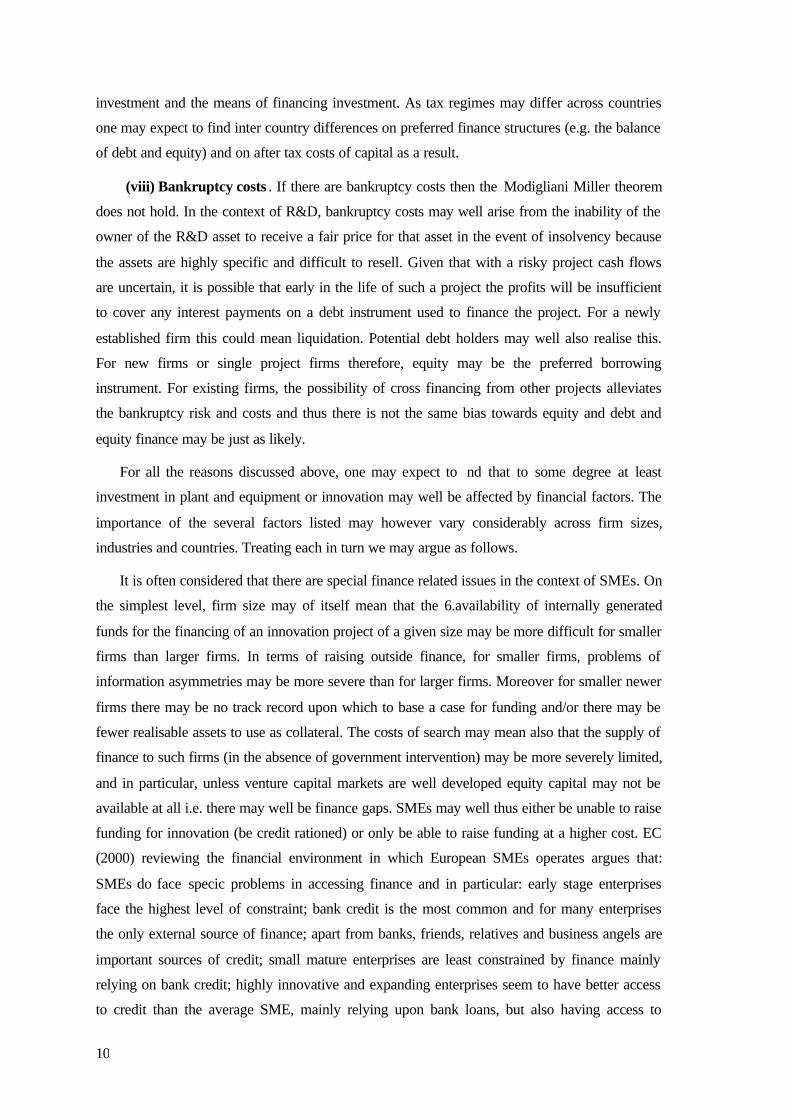
(viii) Bankruptcy costs . If there are bankruptcy costs then the Modigliani Miller theorem
does not hold. In the context of R&D, bankruptcy costs may well arise from the inability of the
owner of the R&D asset to receive a fair price for that asset in the event of insolvency because
the assets are highly specific and difficult to resell. Given that with a risky project cash flows
are uncertain, it is possible that early in the life of such a project the profits will be insufficient
to cover any interest payments on a debt instrument used to finance the project. For a newly
established firm this could mean liquidation. Potential debt holders may well also realise this.
For new firms or single project firms therefore, equity may be the preferred borrowing
instrument. For existing firms, the possibility of cross financing from other projects alleviates
the bankruptcy risk and costs and thus there is not the same bias towards equity and debt and
equity finance may be just as likely.
For all the reasons discussed above, one may expect to nd that to some degree at least
investment in plant and equipment or innovation may well be affected by financial factors. The
importance of the several factors listed may however vary considerably across firm sizes,
industries and countries. Treating each in turn we may argue as follows.
It is often considered that there are special finance related issues in the context of SMEs. On
the simplest level, firm size may of itself mean that the 6.availability of internally generated
funds for the financing of an innovation project of a given size may be more difficult for smaller
firms than larger firms. In terms of raising outside finance, for smaller firms, problems of
information asymmetries may be more severe than for larger firms. Moreover for smaller newer
firms there may be no track record upon which to base a case for funding and/or there may be
fewer realisable assets to use as collateral. The costs of search may mean also that the supply of
finance to such firms (in the absence of government intervention) may be more severely limited,
and in particular, unless venture capital markets are well developed equity capital may not be
available at all i.e. there may well be finance gaps. SMEs may well thus either be unable to raise
funding for innovation (be credit rationed) or only be able to raise funding at a higher cost. EC
(2000) reviewing the financial environment in which European SMEs operates argues that:
SMEs do face specic problems in accessing finance and in particular: early stage enterprises
face the highest level of constraint; bank credit is the most common and for many enterprises
the only external source of finance; apart from banks, friends, relatives and business angels are
important sources of credit; small mature enterprises are least constrained by finance mainly
relying on bank credit; highly innovative and expanding enterprises seem to have better access
to credit than the average SME, mainly relying upon bank loans, but also having access to

11
venture capital and business angels. The theory and such previous empirical findings would thus
suggest that as firm size increases financial factors may well be less important as a constraint
upon innovation.
Differences across industries (for given firm size) may also exist. An obvious consideration
is that in more profitable industries there is less need for external funding than in less profitable
industries. In riskier industries it may be more difficult to raise funding from outside the firm
purely because of the risk factor. In more high tech sectors not only may risk itself be a factor
but also the proportion of assets that are realisable may be lower. In high tech industries
innovation is more likely to be of a sort that has not been undertaken elsewhere before and it
may be particularly difficult to observe the systematic risk of similar projects in other firms
(Goodacre and Tonks, 1995) and thus difficult to determine the appropriate discount rate to use
in evaluating investment in the firm. All such arguments would suggest that in more traditional
industries with extensive track records funding from internal and external sources will be easier.
For more high tech and newer industries funding is more likely to be a problem and thus impact
more upon (constrain) innovative performance.
Differences across countries given firm size and industry are also likely to be apparent.
These may relate to factors such as taxes and subsidy regimes, the completeness of markets for
finance, the legal environment as regards bankruptcy, government intervention etc. Such issues
are part of the national systems of innovation literature (see Nelson, 1993). Part of the national
sys-tem of innovation of particular interest here is the financial environment in different
countries. European financial environment are both heterogeneous and changing (see Stoneman,
2001b). On the one hand in terms of the financial system per se there are bank based systems as
typified by the German situation and on the other market based systems as typified by the UK.
Most continental European systems are largely bank based although there are signs of some
movement in certain countries (e.g. France) to a market based system. Alongside these different
systems there are different patterns of ownership of industry. The German system reflects
greater private ownership, more concentrated ownership and more pyramid ownership. In the
UK the patterns is for less concentrated holding, less private control and few intercorporate
holdings. The different patterns of ownership allied with different financial systems generate
different emphases upon insider and outsider control in the management of corporations. In the
UK type system, although much of the equity may be owned by financial institutions, it is
through the market itself, via the threat of take-over, that control is mainly exercised. In German
type systems there is greater emphasis upon direct intervention by banks and co-operation
between banks and management. The financing of investment by firms also differs across
systems. Although self-generated funds are the main finance source for firms (except SMEs) in
12
all countries these are more important in the UK, with bank finance more important in bank
based systems.
It is argued that the different patterns observed in financial systems have important
implications for the way firms behave. The argument is that bank based systems with insider
control are particularly favourable to longer term steady development built upon the
construction of trust based relations, firm specific investments and steady change but may
generate a higher cost of capital due to bank monopoly power and perhaps undue conservatism.
On the other hand market based systems with outsider control and more arms length
relationships between the financiers and the managers are seen as more favourable to major
change and switches of strategic direction but encouraging liquidation of investment in the
event of dissatisfaction with no obligation to take anything other than a short term view. It is not
however being suggested that one system is better than another, it is more a matter of “horses
for courses”. It would be a surprise however if different national financial systems did not
impact upon innovative behaviour. This is easy to accept. What is more difficult to predict is the
direction and importance of that impact. A particular interest in the literature is the differences
of impact between Anglo American market based systems and German- Japanese bank based
systems.
Bond et al.(1997) find that the sensitivity of investment to financial variables is
quantitatively more significant in the UK than in France, Germany or Belgium 1978 – 1989.
This is interpreted as a particular failing of the market orientated UK system. Mulkay, Hall and
Mairesse (2000) undertake a similar cross country comparison, but this time for both R&D and
investment and between the US and France. Again significant differences are found across the
two countries with a greater importance of profit or cash flow as a determinant of investment in
the US than in France, however any differences are much less obvious when it comes to R&D.
Between 1982-1993, for investment, cash flow did not matter for French firms at all but
significantly affected the investment of US firms. The authors argue that this is probably the
result of real differences in the working of capital markets in the two countries. In particular
they argue that US shareholders were some-what more likely to sell their shares in adverse
situations providing greater market discipline and thus more rapid responsiveness of US firms to
changes in their prospects. To the extent that US firms feel pressure to use internal funds to
finance future spending, they will have a higher long run response to surprises in profits (not
accompanied by surprises in demands) than would otherwise be the case.
This review of the theoretical arguments and (some) empirical literature indicates that one
might expect to find that financial factors do impinge upon innovative activity. One might also
expect that this impact will be greater for small and medium sized firms than for large firms.
The impact will also differ across industries with more risky, newer industries experiencing

13
greater problems. There may also be differences across countries although theoretically it is
difficult to predict the nature of the differences. Past empirical work suggests that market based
systems may experience the greatest problems. In the next section we consider the CISII data
that we will be using to explore these issues further in the later sections.

15
2 DATA DESCRIPTION
The data source used in this paper is the Second Community Innovation Survey (CIS II).
This pan European firm-level survey was conducted (largely by national statistical offices)
under the auspices of the European Innovation Monitoring System (EIMS) and Eurostat in
1997, so that the reference year for the survey is 1996 for most of the sample countries
(although Norway and Portugal refer to 1997) 1. The survey was designed on the basis of an
harmonised questionnaire applied in each country, making the data-set suitable for cross country
comparison. The countries included in the survey are Belgium, Denmark, Germany, Spain,
France, Ireland, Italy, Luxembourg, Netherlands, Austria, Portugal, Finland, Sweden, UK, and
Norway with firms in each country classified by industry (11 manufacturing sectors, six service
sectors) and by firm size class (small, medium and large, defined respectively as firms with 20
to 49 employees in the manufacturing sector (10 to 49 in the service sector), 50 to 249
employees and more than 250 employees). Unfortunately, to preserve firms’ confidentiality,
firm level data was not available to us, the data used here is instead at the industry, country or
firm class level of aggregation.
The section of the CISII questionnaire of most interest to us concerns the factors hampering
innovation. The question asked is reproduced below.
1 A prior Community Innovation Survey (CIS I) was undertaken in 1993. Unfortunately, itsuffered from both country-specific problems (e.g. the response rate in some country was so lowthat the results could not be published) and “cross-country” problems (e.g. in some countriesfirms were selected according to the principle of random sampling, in other countries the censuswas used, while a third category of countries defined a sample of likely innovators). We thuselected to concentrate in this paper on CIS II.

16
The innovation activity of your company could be hampered by various factors which might
prevent innovation projects or slow up or stop projects in progress
a) Has at least one innovation project in 1994 – 1996 been
yes no
- seriously delayed
- abolished
- not even started
b) If yes on at least one question, tick the relevant factors in the respective columns
Hampering factors
seriously abolished not even
delayed started
1. Excessive perceived economic risks
2. Innovation costs too high
3. Lack of appropriate sources of finance
4. Organisational rigidities
5. Lack of qualified personnel
6. Lack of information on technology
7. Lack of information on markets
8. Fulfiling regulations, standards
9. Lack of customer responsiveness
The data available to us on the responses to this question are the proportions (relative to the
number of firms reporting some innovative activity in the sample) for each impact (delay,
abolish, not start) by country and firm size class and by country and industry (not by country,
industry and firm size class). In the sections below we undertake two exercises with this data. In
the first we are interested in how important are financial factors as opposed to other hampering
factors as a constraint upon innovation in terms of their impact in leading to delay, abandonment
or not starting innovation projects. In the second exercise we concentrate solely upon hampering
factor 3 and explore more fully the nature of the financial constraints across firm size classes,
industries and countries. In the next section we briefly summarise the econometric method to be
used.

17
3 THE ECONOMETRIC MODEL
The econometric method we used below is known as a Generalized Linear Model ((GLM here
afterward). We refer the reader to McCullagh and Nelder (1989), Cox and Snell (1989), and
Dobson (1990) for a detailed treatment of such models. The class of GLM can be considered as
an extension of the classical linear model. In the classical linear regression model it is assumed
that
iii XY εβ += ' (1)
where the elements of iε are assumed to be i.i.d. N (0, 2σ ), iX is a matrix of non correlated
explanatory variables, and β is a vector of parameters. Compared to this framework GLM
allows two generalisations. Firstly, the relationship between the response variable iY and the
explanatory variables in iX need not to be of the simple linear form incorporated in (1), but
may be distributed as any monotonic differentiable function. Secondly, the iY does not need to
have a Normal distribution, but may come from an exponential family.
In our case we consider n independent random variables iY corresponding to the number of
successes in the n different subgroups (e.g. different firm size class). Therefore, the dependent
variable iY is a binary random variable which assumes value one with probability
π== )0(YPr and value zero with probability π−== 1)0(YPr 2. To model the probability
π we need to specify the functional form of
2 Consider a random variable Y whose probability density function depends only on a singleparameter θ . This distribution belong to the exponential family if it can be written in the form
,)()(),( )()( θθθ byaetysyf =
where a, b, s and t are known functions. This equation can be rewritten in the form
[ ][ ],)()()()(exp
)()()(log)(logexp),(ydcbya
byatysyf++=
++=θθ
θθθ
where )(exp)( ydys = and )(exp)( θθ ct = . The binomial distribution belongs to theexponential family since the distribution

18
βπ ')( Xg =
where )(⋅g is a monotonic differentiable function. Moreover, we need to ensure that π is
bounded between zero and one. That is we need to choose a cumulative probability distribution
such that
∫∞−
− ==x
dzzfXg )()'(1 βπ
where 0)( ≥zf and ∫∞
∞−
=1)( dzzf . Our choice of )(zf is
)'exp(1)'exp(
)(β
βπ
XX
dzzfx
+== ∫
∞−
(2)
and taking the logit transformation we can write equation (2) as
.'1
)( βπ
ππ Xg =
−= (3)
In the literature model (2) is usually referred to as the logit model or sometimes as logistic
regression. To estimate the model we use maximum likelihood, the log-likelihood function for
(3) being given by
( ) ynyi y
nyf −−
= πππ 1),(
where i= 1,…,n, can be written as
( ) ( )
+−+−−=
yn
nyyyf i log1log1loglogexp),( ππππ
which is the form above.

19
( ) .log11
log),(1
∑=
+−+
−=
n
iiiii y
nynyyL π
ππ
π
Maximising this function with respect to the vector β and equating the resulting
expressions to zero yields estimates of the unknown parameters. To measure the goodness of fit
of the model we use the likelihood ratio test statistic given by
( )[ ] );ˆ(;ˆ2 max ylylD ππ −=
where maxπ̂ is the vector of maximum likelihood estimates corresponding to the maximal model
and π̂ is the vector of maximum likelihood estimates for our model. Another criteria of
goodness of t is given by the Pearson 2χ statistic. This test statistic is derived by minimizing
the weight sum of squares
( )( )∑
= −−
=n
i iii
iiiw n
nyS
1
2
ˆ1ˆˆππ
π
since iii nYE π=)( and )1()(2iiii nY ππσ −−= which is asymptotically distributed as 2χ a
distribution. Other measures of goodness of t are the Akaike (1973) information criterion (AIC),
and the Bayesian information criterion (BIC) (Raftery (1996)).

21
4 THE IMPORTANCE OF FINANCIAL FACTORS
In this section we explore the importance in hampering innovation of financial and related
cost and risk factors relative to the other hampering factors. The exercise is performed using
data from 12 sample EU countries, it being necessary on the grounds of data deficiencies to
drop Spain, Portugal and Luxembourg from the original sample of 15. The data allows a
distinction between services and manufacturing and thus we also allow a two way industry split.
The basic approach is to separately consider for each impact (delay, abandonment, not start), the
proportion of sample firms in each of the two industry sectors in each country who report such
an impact, and to relate that to the hampering factors reported. Defining i as representing impact
(i = 1,…,3), j as the hampering factor (j = 1,…,9) and m as the industry (m=1,2), the dependent
variable, for each i, ( ijmoutinn _ ), is the proportion of firms in industry m in each country
reporting hampering factor j as having impact i. For each i there are 216 observations upon ijm
(m times j times 12 countries). The explanatory variables are the nine factors hampering
innovating reported in the previous section . Therefore, the estimated equation for each i is
,_ ,,
1
1,,0 mij
j
jmijjijm Facoutinn εβα ++= ∑
−
=
(4)
where the right hand side variables are dummy variables that take the value of unity when the
data point relates to that factor and zero otherwise (in the estimates we keep Factor 9 as a
baseline). The estimated parameters, for each i, provide, in essence, an average across industries
and countries of the relative importance of the nine different factors in hampering innovation. In
the tables that immediately follow we report the estimated coefficients for equation (4), relating
respectively to projects delayed (Table 1), abolished (Table 2), and not started (Table 3).
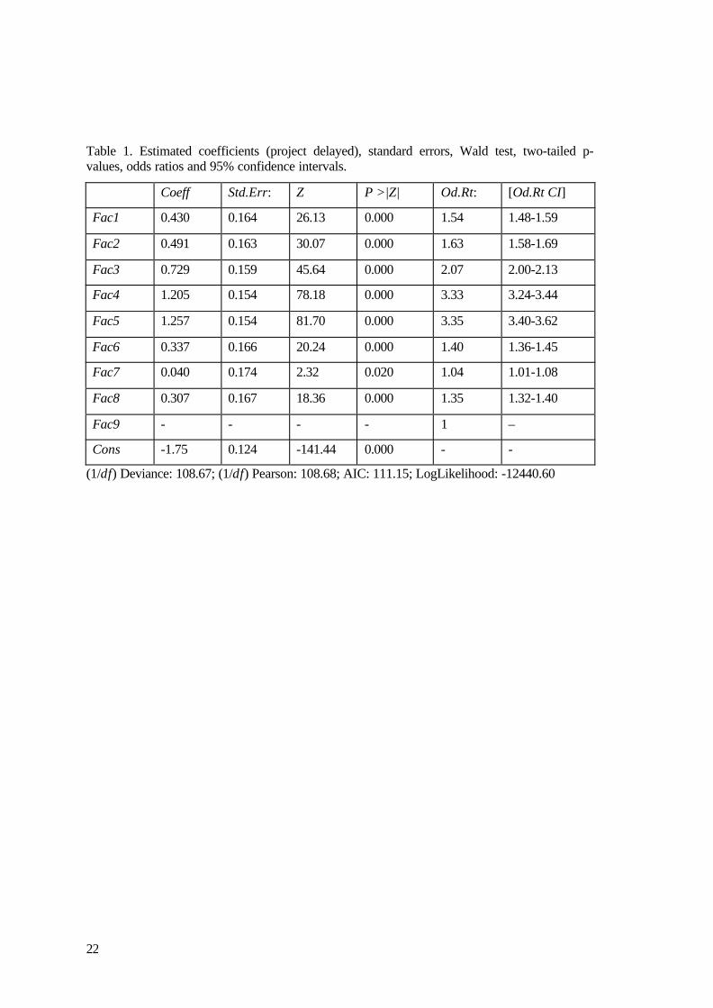
In terms of the goodness of t, the Wald tests reported in Tables 1-3 indicate that the right
hand side variables are highly significant in each case, moreover the relative p-values are close
to zero. However, the AIC criteria is lower for projects abolished as a dependent variable,
implying that the model better fits the data on delayed and not started projects.
22
Table 1. Estimated coefficients (project delayed), standard errors, Wald test, two-tailed p-values, odds ratios and 95% confidence intervals.
Coeff Std.Err: Z P >|Z| Od.Rt: [Od.Rt CI]
Fac1 0.430 0.164 26.13 0.000 1.54 1.48-1.59
Fac2 0.491 0.163 30.07 0.000 1.63 1.58-1.69
Fac3 0.729 0.159 45.64 0.000 2.07 2.00-2.13
Fac4 1.205 0.154 78.18 0.000 3.33 3.24-3.44
Fac5 1.257 0.154 81.70 0.000 3.35 3.40-3.62
Fac6 0.337 0.166 20.24 0.000 1.40 1.36-1.45
Fac7 0.040 0.174 2.32 0.020 1.04 1.01-1.08
Fac8 0.307 0.167 18.36 0.000 1.35 1.32-1.40
Fac9 - - - - 1 –
Cons -1.75 0.124 -141.44 0.000 - -
(1/df) Deviance: 108.67; (1/df) Pearson: 108.68; AIC: 111.15; LogLikelihood: -12440.60
23
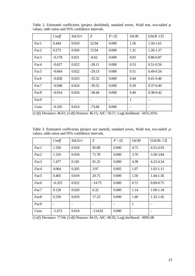
Table 2. Estimated coefficients (project abolished), standard errors, Wald test, two-tailed p-values, odds ratios and 95% confidence intervals.
Coeff Std.Err Z P>|Z| Od.Rt [Od.R. CI]
Fac1 0.444 0.019 22.94 0.000 1.56 1.50-1.61
Fac2 0.273 0.020 13.94 0.000 1.31 1.26-1.37
Fac3 -0.178 0.021 -8.62 0.000 0.83 0.80-0.87
Fac4 -0.627 0.022 -28.11 0.000 0.53 0.51-0.56
Fac5 -0.664 0.022 -29.53 0.000 0.51 0.49-0.54
Fac6 -0.828 0.023 -35.52 0.000 0.44 0.41-0.46
Fac7 -0.948 0.024 -39.52 0.000 0.39 0.37-0.40
Fac8 -0.914 0.024 -38.44 0.000 0.40 0.38-0.42
Fac9 - - - - 1 –
Cons -0.105 0.014 -73.84 0.000 - -
(1/df) Deviance: 46.61; (1/df) Pearson: 46.15; AIC: 50.57; LogLikelihood: -5655.2016.
Table 3. Estimated coefficients (project not started), standard errors, Wald test, two-tailed p-values, odds ratios and 95% confidence intervals.
Coeff Std.Err: Z P >|Z| Od.Rt [Od.Rt. CI]
Fac1 1.550 0.018 85.89 0.000 4.75 4.55-4.93
Fac2 1.310 0.018 71.78 0.000 3.70 3.58-3.84
Fac3 1.477 0.181 81.25 0.000 4.38 4.23-4.54
Fac4 0.064 0.205 3.97 0.002 1.07 1.02-1.11
Fac5 0.405 0.019 20.75 0.000 1.50 1.44-1.56
Fac6 -0.325 0.022 -14.75 0.000 0.72 0.69-0.75
Fac7 0.128 0.020 6.32 0.000 1.14 1.09-1.18
Fac8 0.339 0.019 17.23 0.000 1.40 1.35-1.45
Fac9 - - - - 1 –
Cons -1.672 0.014 -114.02 0.000 - -
(1/df) Deviance: 77.94; (1/df) Pearson: 84.55; AIC: 80.92; LogLikelihood: -9095.08
24
In the last two columns of Table 1-3 we report the odds ratios and their relative confidence
interval. The odds ratios are defined as
odds ratio ),ˆexp( iβ=
and the confidence intervals are calculated in the same way from the 95% confidence interval of
iβ̂ .
The main purpose of this exercise is to explore the relative importance of different factors in
hampering innovation. In terms of the odds ratios we may observe that for projects not started
and for projects abolished the dominant hampering factors are 1-3. These factors are still
important in delaying projects but there factors 4 and 5 are relatively more important. Factor 3, a
lack of appropriate sources of finance, is a dominant factor in projects not started and an
important factor in causing delay but is relatively less important in leading to projects being
abolished. This would make some sense if one considers that firms will not start projects if
financing is not likely to be available and thus abandonment on financial grounds will be
uncommon (as might be delay). There thus seems clear evidence that (especially as regards not
starting projects) that financial factors are relatively important. This result is further emphasised
if we group the hampering factors into three sub groups, the first covering factors 1-3 which we
label finance, costs and risks (hereafter FCR), the second covering 4-7 (i.e. organisational
rigidity, lack of qualified personnel, lack of information on technology, lack of information on
markets) which we label internal factors and the third covering 8 and 9 ( fulfilling regulations
and standards, lack of customer responsiveness to new products) which we label external
factors. In Appendix Table 1A we present the correlation matrix across the nine factors. The full
impact of financial factors may well be better represented by the impact of the whole FCR
group rather than just factor 3. We see for example that in terms of not starting projects, the
FCR factors are 3-4 times as important as any other factor. In firms of abolishing projects,
although factor 3 itself, a lack of appropriate finance is not that important, the FCR factors in
total are more important than other factors. In firms of delaying projects, the FCR factors are
important but not as important as factors 4 and 5. The results lead us to conclude that a lack of
appropriate sources of finance is a major hampering factor to innovation. The effect is most
notice-able in terms of causing innovation projects to not be started. If financial factors are
interpreted more widely to also encompass excessive risk and innovation costs too high then this
result is further emphasised. As the sample is made up of firms that have actually recorded some
innovative activity (non innovators are not even included in the sample) our results may even
underestimate, in an absolute sense, the impact of finance as a barrier to innovation.
25
5 FINANCIAL CONSTRAINTS BY FIRMSIZE AND COUNTRY
Having established the relative importance of financial constraints as a barrier to innovation,
in this section we focus on the third hampering factor listed in the CISII questionnaire and
reported in Section 2: this relates specifically to a lack of appropriate sources of finance (Fac3
here afterward). In particular, we consider, for the same sample of twelve EU Member States,
whether the importance of Factor 3 varies across countries and firm size. Defining i as before, as
representing impact (i = 1,…,3), k (k = 1,…,3) as the size class (small, medium large) and l as
the country (l =1,…,12), the dependent variable for this analysis ( ikloutinn _ ) is the proportion
of firms (who record some innovative activity) in a country in a size class who report impact i
from hampering factor 3. This provides a total of 108 data points. The right hand side variables
are 12 dummy variables for country, 3 for size class and 3 for impact that take values of one or
zero to match the data point, plus a number of interactive dummies between countries and firm
size to pick up different effects of size in different countries. In modelling this relationship we
sought the most parsimonious model that still explained the data. The rationale for minimising
the number of explanatory variables was to produce a more numerically stable model. It is well
known (see for example Harrel et al. (1996) or Hosmer and Lemeshow (2000)) that the more
variables are included in a model, the greater the estimated standard errors become, and the
more dependent the model becomes on the observed data. The criteria followed for including or
excluding a variable from the final model was based on the likelihood ratio.
The estimates were generated with large firms, projects delayed, and Germany incorporated
in the base line. Initial estimates using a likelihood ratio test and the Wald test statistic for each
variable led us to drop several country dummies from our initial model3. The results of adding
21 interaction dummies (i.e. 3 firm classes times the remaining 7 country dummies with
Germany in the base-line) one at a time to the model is shown in the Appendix (Table 2A). Our
choices as to which of these remains in the final preferred estimates was based upon the
likelihood ratio test
3 The country variables not significant are: Belgium (Wald test=0.82 and p-value=0.412 , LRtest: )1(2χ =1.62 p-value=0.4450); Denmark (Wald test=1.26 and p-value=0.206 , LR test:
)1(2χ =1.05 p-value=0.3047); Netherlands (Wald test=0.59 and p-value=0.557 , LR test:
)1(2χ =0.34 p-value=0.5580); Austria: (Wald test=1.22 and p-value=0.224 , LR test:
)1(2χ =1.56 p-value=0.2578).

26
−=
jariableeraction vhe del with t of the molikelihoodcts model main effelikelihood
LR int
ln2
for j=1,…,21 which is asymptotically distributed as a 2χ with j degrees of freedom. We include
in the final model only those interactions which are significant at the 5% level or 10% at most
(see Table (2A) in the Appendix). In Table 4a we present the estimated parameters and some
goodness of t tests.
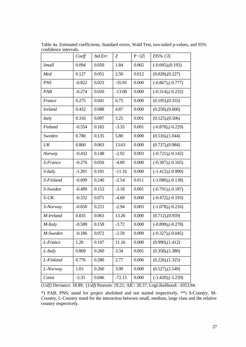
27
Table 4a. Estimated coefficients, Standard errors, Wald Test, two-tailed p-values, and 95%confidence intervals.
Coeff Std.Err. Z P >|Z| [95% CI]
Small 0.094 0.050 1.84 0.065 (-0.005),(0.193)
Med 0.127 0.051 2.50 0.012 (0.028),(0.227)
PNS -0.822 0.023 -35.95 0.000 (-0.867),(-0.777)
PAB -0.274 0.020 -13.08 0.000 (-0.314),(-0.232)
France 0.275 0.041 6.75 0.000 (0.195),(0.355)
Ireland 0.432 0.088 4.87 0.000 (0.258),(0.606)
Italy 0.316 0.097 3.25 0.001 (0.125),(0.506)
Finland -0.554 0.165 -3.35 0.001 (-0.878),(-0.229)
Sweden 0.780 0.135 5.80 0.000 (0.516),(1.044)
UK 0.860 0.063 13.63 0.000 (0.737),(0.984)
Norway -0.432 0.148 -2.92 0.003 (-0.721),(-0.142)
S-France -0.276 0.056 -4.89 0.000 (-0.387),(-0.165)
S-Italy -1.201 0.101 -11.16 0.000 (-1.412),(-0.990)
S-Finland -0.699 0.240 -2.54 0.011 (-1.080),(-0.138)
S-Sweden -0.489 0.153 -3.18 0.001 (-0.791),(-0.187)
S-UK -0.332 0.071 -4.68 0.000 (-0.472),(-0.193)
S-Norway -0.650 0.221 -2.94 0.003 (-1.078),(-0.216)
M-Ireland 0.835 0.063 13.26 0.000 (0.712),(0.959)
M-Italy -0.589 0.158 -3.72 0.000 (-0.899),(-0.278)
M-Sweden -0.186 0.072 -2.59 0.009 (-0.327),(-0.045)
L-France 1.20 0.107 11.16 0.000 (0.990),(1.412)
L-Italy 0.869 0.260 3.34 0.001 (0.358),(1.380)
L-Finland 0.776 0.280 2.77 0.006 (0.226),(1.325)
L-Norway 1.03 0.260 3.99 0.000 (0.527),(1.549)
Const -3.33 0.046 -72.15 0.000 (-3.420),(-3.239)
(1/df) Deviance: 18.89; (1/df) Pearson: 19.21; AIC: 20.37; LogLikelihood: -1053.84.
*) PAB, PNS; stand for project abolished and not started respectively. **) S-Country, M-Country, L-Country stand for the interaction between small, medium, large class and the relativecountry respectively.
28
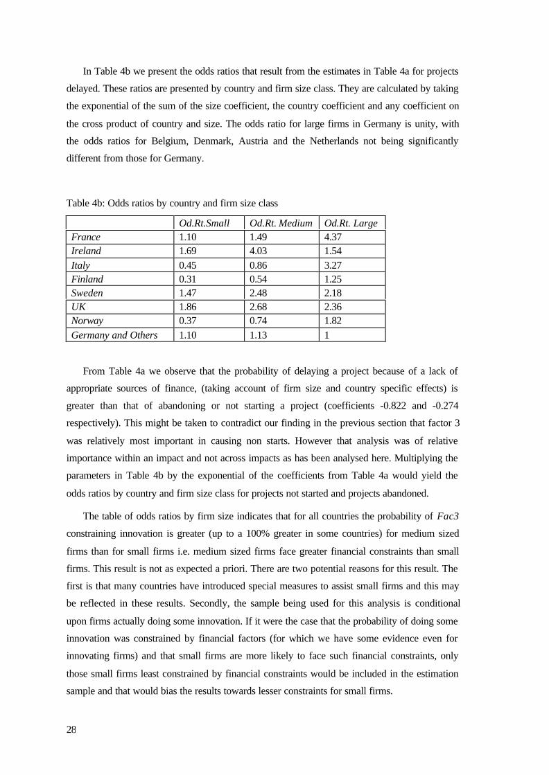
In Table 4b we present the odds ratios that result from the estimates in Table 4a for projects
delayed. These ratios are presented by country and firm size class. They are calculated by taking
the exponential of the sum of the size coefficient, the country coefficient and any coefficient on
the cross product of country and size. The odds ratio for large firms in Germany is unity, with
the odds ratios for Belgium, Denmark, Austria and the Netherlands not being significantly
different from those for Germany.
Table 4b: Odds ratios by country and firm size class
Od.Rt.Small Od.Rt. Medium Od.Rt. LargeFrance 1.10 1.49 4.37Ireland 1.69 4.03 1.54Italy 0.45 0.86 3.27Finland 0.31 0.54 1.25Sweden 1.47 2.48 2.18UK 1.86 2.68 2.36Norway 0.37 0.74 1.82Germany and Others 1.10 1.13 1
From Table 4a we observe that the probability of delaying a project because of a lack of
appropriate sources of finance, (taking account of firm size and country specific effects) is
greater than that of abandoning or not starting a project (coefficients -0.822 and -0.274
respectively). This might be taken to contradict our finding in the previous section that factor 3
was relatively most important in causing non starts. However that analysis was of relative
importance within an impact and not across impacts as has been analysed here. Multiplying the
parameters in Table 4b by the exponential of the coefficients from Table 4a would yield the
odds ratios by country and firm size class for projects not started and projects abandoned.
The table of odds ratios by firm size indicates that for all countries the probability of Fac3
constraining innovation is greater (up to a 100% greater in some countries) for medium sized
firms than for small firms i.e. medium sized firms face greater financial constraints than small
firms. This result is not as expected a priori. There are two potential reasons for this result. The
first is that many countries have introduced special measures to assist small firms and this may
be reflected in these results. Secondly, the sample being used for this analysis is conditional
upon firms actually doing some innovation. If it were the case that the probability of doing some
innovation was constrained by financial factors (for which we have some evidence even for
innovating firms) and that small firms are more likely to face such financial constraints, only
those small firms least constrained by financial constraints would be included in the estimation
sample and that would bias the results towards lesser constraints for small firms.

29
Turning to comparisons of large firms to small and medium sized firms, the data in Table 4b
indicates that: in France, Italy, Finland, and Norway, large firms are more likely to experience
financial constraints than small and medium sized firms; in Sweden and the UK large firms are
more likely to face financial constraints than small but not medium sized firms; in Ireland large
firms are less likely to face financial constraints than both small and medium sized firms. The a
priori expectation was that large firms would be least constrained and the data does not clearly
support this view. Once again this could be because the sample is conditional upon firms
actually undertaking some innovative activity and the presence of government assistance
schemes to SMEs.
These results could also be reflecting different size compositions for firms in different
industrial sectors. If, as we explore in the next section, firms in different sectors face different
levels of financial constraints, and the average firms size differs across sectors, then the results
in Table 4b could be reflecting this. Unfortunately our data does not allow decomposition by
country size and sector.
The analysis of the odds ratios in Table 4b by country reveals significant differences. For
small firms, those in the UK have the highest probability of facing financial constraints, some
70% greater than in Germany. Small firms in Ireland and Sweden also have high odds ratios.
Small firms in other countries have odds ratios either the same as or less than German firms. For
medium sized firms, Irish firms stand out as having a particularly high odds ratio but Swedish
and UK firms again have relatively high odds ratios. Italy Finland and Norway show
(internationally relatively) low odds ratios for medium sized firms. For large firms, in France
the odds ratio is 430% higher than in Germany, and also high in Italy, the UK and Sweden. All
other countries show odds ratios greater than or equal to Germany. Thus, as far as large firms
are concerned, the German financial environment is particularly favourable.
One explanation for these results may be based on the distribution of the enterprises by
technological sector. According to the CISII results Ireland, UK, and Sweden are the countries
with the highest shares of enterprises in the high-tech sector, while Germany has a strong
position in the medium-high and medium-low branches. In general the share of innovating firms
in a sector is higher, the higher is the sector’s level of technology. As we will see in the next
section high-tech enterprises are the ones more likely to experience financial constraints.
Therefore, to some extent, it seems reasonable to argue that the results in Table 4b are affected
to some degree by the distribution of the enterprises according to the level of technology of the
countries considered.
Having said this however, in the theoretical section we argued that one might well expect
financial constraints to have differing impacts in different countries although it was difficult to

30
predict a priori exactly in which countries the constraints would be most severe. However it was
suggested on the basis of previous empirical work that firms in countries with market based
systems as opposed to bank based systems would experience more financial constraints and a
comparison of the UK to Germany could be taken as an indicator of this. It is clear that for all
three firm size classes, the odds ratios is greater in the UK than in Germany and this may be
support for the view that market based systems are more likely to constrain innovation.
However only for small sized firms is the UK odds ratio the largest estimated. For medium
sized firms Ireland has a higher ratio and for large firms Italy and France have higher ratios.
Given that many factors other than whether systems are market based or bank based is likely to
affect these ratios one cannot be definitive, but as the UK odds ratios rank as numbers 1, 2 and 3
(out of 12) for small, medium and large sized firms respectively, the circumstantial evidence
that there are particular financial constraints in the UK compared to all other European, largely
bank based, countries is strong. One might also note the empirical evidence quoted in section 2
above compared the UK to France, Belgium and Germany suggesting that financial factors were
more important in the UK as a constraint upon investment. Our findings corroborate this except
for large firms in France.
31
6 FINANCIAL CONSTRAINTS BY INDUSTRY
Having explored the relationship between financial constraints and firm size by country, in
this final section we explore inter industry differences in the importance of financial constraints.
Again we restrict ourselves to the importance of Factor 3, a lack of appropriate source of
finance. To see if our results are consistent with the ones in Section 6, we introduce as
explanatory variables in the model not only industry dummies, but also country dummies.
Defining i as representing impact (i=1,...,3), l as the country (l=1,…,12), and m as the industry,
the dependent variable for this analysis ( imloutinn _ ) is the proportion of firms in a country in
an industry who report impact i from hampering factor 3. Unfortunately, we are severely
constrained by data availability and this has led us first to consider only two impacts i.e. projects
not started and projects delayed. We analyse these separately rather than together for reasons
that will become apparent below. There are many gaps in the data at the industry level
especially for the service sectors. Therefore, there is a trade-off between considering a larger
number of countries but a smaller number of industries, or the opposite. Given the aim of the
experiment, we have decided to reduce the number of countries considered in order to maximise
the number of industries included in the model. Following this criteria our final data set contains
12 industries, and 9 countries for “project delayed” (i.e. 108 data points), and 8 countries and
fourteen industries (102 data points) for “project not started”4. The right hand side variables in
each regression are industry and country dummy variables that take the value of unity when the
data point relates to that industry or country and zero elsewhere. The industry definitions are
listed in Table 3A (see appendix).
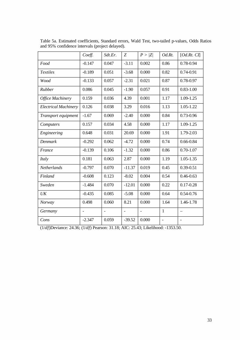
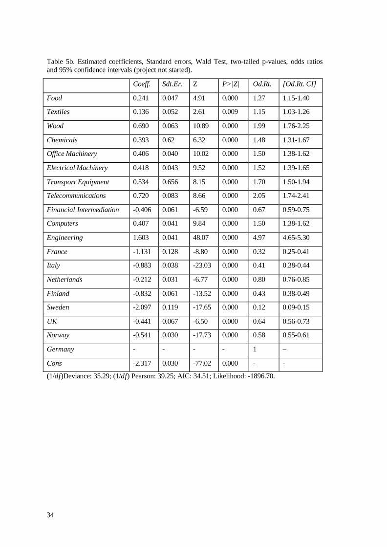
In Table 5a and 5b we report the estimated coefficients for projects delayed and projects not
started, respectively 5. The industry chosen as a base line is “Manufacture of basic metals and
fabricated metal products”, a rather traditional industry. As far as the country variables are
4 The countries considered for “project delayed” are Germany, France, Italy, Nether-lands,Finland, Sweden, UK, Norway for the sectors described in Table 5a, while for “project notstarted” we include Denmark but we do not include the following industries: “electricity” and“telecommunication”.5 In Table 5a we do not include the following explanatory variables: “Chemicals” (estimatedparameter=0.02, Wald test=0.39 (p-value=0.70)) “Transport” (estimated parameter=-0.04, Waldtest= -1.16 (p-value=0.247)). For the restricted model the LR test gives: )2(2χ =2.32; (p-value=0.31) : While in Table 5b we do not include: “Rubber” (estimated parameter=0.07, Waldtest= 1.53 (p-value=0.20)) “Electricity” (estimated parameter= 0.19, Wald test=1.01 (p-value=0.31)). For the restricted model the LR test gives: )2(2χ =1.90; (p-value=0.38).

32
concerned, to be consistent with the model in Section 6 we keep Germany as a base line. From
Table 5a-b, we can see that the majority of the country odds ratios are less then one, meaning
that the probability of having financial constraints for the countries analysed is less then the
probability of having the same problem in Germany. The apparent inconsistency of this result
with those reported in Table 4b can be explained by considering that, even though we do not
know the characteristics of the firms in the industries, the proportion of the class “small firm” in
the sample is much bigger then the medium and large firm classes (the approximate sample
composition is 60:30:10, small, medium, large). The sample is also unbalanced across countries
with for example Italy being over represented. It is likely that the results we find reflect the
composition of our sample and as seen in Table 4b, the odds ratios for small firms are generally
less than for large firms and often less than unity. The odds ratios in Table 5a are not
inconsistent with those for small firms re-ported in Table 4b.
From Tables 5a and 5b it emerges that there are significant differences across industries in
the importance of financial constraints and impacts on delay and non starts are also different
across industries. Our theoretical discussion suggested that firms in newer, riskier and less
profitable industries are likely to experience more financial constraints than in other industries.
We observe that in “Computers” and “Engineering” which might be considered newer and
riskier industries, the odds ratio is particularly high for both projects delayed and not started. In
“telecommunications” which again might be considered newer and higher tech, firms are more
than twice as likely to not start an innovating project as in “Manufacture of basic metal”. In
more traditional sectors such as Food, Textiles and Rubber the odds ratios are relatively small
(although it is difficult to explain why Wood carries a high ratio in Table 5b). In Financial
Intermediation which might be considered a more profitable industry, the probability of not
starting an innovating project because of lack of financial resources at 0.67 is less than in the
base industry.
To the extent that it is possible to draw conclusions from such patterns therefore, it would
appear that the findings are consistent with the view that high tech and high risk imply greater
financial constraints than low tech, low risk, and also that high profitability means fewer
financial constraints.
33
Table 5a. Estimated coefficients, Standard errors, Wald Test, two-tailed p-values, Odds Ratiosand 95% confidence intervals (project delayed).
Coeff. Sdt.Er. Z P > |Z| Od.Rt. [Od.Rt. CI]
Food -0.147 0.047 -3.11 0.002 0.86 0.78-0.94
Textiles -0.189 0.051 -3.68 0.000 0.82 0.74-0.91
Wood -0.133 0.057 -2.31 0.021 0.87 0.78-0.97
Rubber 0.086 0.045 -1.90 0.057 0.91 0.83-1.00
Office Machinery 0.159 0.036 4.39 0.001 1.17 1.09-1.25
Electrical Machinery 0.126 0.038 3.29 0.016 1.13 1.05-1.22
Transport equipment -1.67 0.069 -2.40 0.000 0.84 0.73-0.96
Computers 0.157 0.034 4.58 0.000 1.17 1.09-1.25
Engineering 0.648 0.031 20.69 0.000 1.91 1.79-2.03
Denmark -0.292 0.062 -4.72 0.000 0.74 0.66-0.84
France -0.139 0.106 -1.32 0.000 0.86 0.70-1.07
Italy 0.181 0.063 2.87 0.000 1.19 1.05-1.35
Netherlands -0.797 0.070 -11.37 0.019 0.45 0.39-0.51
Finland -0.608 0.123 -8.02 0.004 0.54 0.46-0.63
Sweden -1.484 0.070 -12.01 0.000 0.22 0.17-0.28
UK -0.435 0.085 -5.08 0.000 0.64 0.54-0.76
Norway 0.498 0.060 8.21 0.000 1.64 1.46-1.78
Germany - - - - 1 –
Cons -2.347 0.059 -39.52 0.000 - -
(1/df)Deviance: 24.36; (1/df) Pearson: 31.18; AIC: 25.43; Likelihood: -1353.50.
34
Table 5b. Estimated coefficients, Standard errors, Wald Test, two-tailed p-values, odds ratiosand 95% confidence intervals (project not started).
Coeff. Sdt.Er. Z P>|Z| Od.Rt. [Od.Rt. CI]
Food 0.241 0.047 4.91 0.000 1.27 1.15-1.40
Textiles 0.136 0.052 2.61 0.009 1.15 1.03-1.26
Wood 0.690 0.063 10.89 0.000 1.99 1.76-2.25
Chemicals 0.393 0.62 6.32 0.000 1.48 1.31-1.67
Office Machinery 0.406 0.040 10.02 0.000 1.50 1.38-1.62
Electrical Machinery 0.418 0.043 9.52 0.000 1.52 1.39-1.65
Transport Equipment 0.534 0.656 8.15 0.000 1.70 1.50-1.94
Telecommunications 0.720 0.083 8.66 0.000 2.05 1.74-2.41
Financial Intermediation -0.406 0.061 -6.59 0.000 0.67 0.59-0.75
Computers 0.407 0.041 9.84 0.000 1.50 1.38-1.62
Engineering 1.603 0.041 48.07 0.000 4.97 4.65-5.30
France -1.131 0.128 -8.80 0.000 0.32 0.25-0.41
Italy -0.883 0.038 -23.03 0.000 0.41 0.38-0.44
Netherlands -0.212 0.031 -6.77 0.000 0.80 0.76-0.85
Finland -0.832 0.061 -13.52 0.000 0.43 0.38-0.49
Sweden -2.097 0.119 -17.65 0.000 0.12 0.09-0.15
UK -0.441 0.067 -6.50 0.000 0.64 0.56-0.73
Norway -0.541 0.030 -17.73 0.000 0.58 0.55-0.61
Germany - - - - 1 –
Cons -2.317 0.030 -77.02 0.000 - -
(1/df)Deviance: 35.29; (1/df) Pearson: 39.25; AIC: 34.51; Likelihood: -1896.70.

35
7 CONCLUSION
There is a growing literature upon the extent to which financial factors con-strain
investment and innovation within firms. In this paper we have explored questionnaire data taken
for the second Community Innovation Survey to ad-dress the role of financial factors in the
determination of innovative activity within Europe. The theoretical literature suggests that
financial factors will constrain such activity, but the importance of such constraints will vary ac-
cording to characteristics of national financial environments, firm sizes and industrial sectors.
Using a generalised linear econometric model we initially nd that, of the several factors that
could constrain innovative activity in Europe, financial factors, especially a lack of an
appropriate source of finance, are the most important, generally outweighing the importance of
other internal and external factors in causing projects to be delayed, abandoned or not started.
Exploring the role of a lack of appropriate sources of finance further we discovered
significant differences between countries, firm size classes and industries in the extent to which
the constraint binds. Theoretical predictions and past empirical work suggested that market
based financial systems are likely to generate more severe financial constraints than bank based
systems. Comparisons of the UK with other countries (especially Germany) confirmed this
prediction. We also found evidence that higher risk, newer, less profitable industries are more
likely to experience financial constraints. We found little evidence however that smaller firms
are more financially constrained than larger firms, although there may be sample bias based
reasons for this.
In the next few moths the results from the third Community Innovation Survey will be
available. It is our intention to extend this work by exploring these issue upon that data set,
which will also provide a time dimension to this study.


37
REFERENCES
[1] Akaike, H. (1973). Information theory and an extension of the maximum likelihoodprinciple. In Second international symposium on infofirmation theory, ed. Petrov B.N. andCsaki F. 267-281. Budapest: Akademei Kiado.
[2] S. Bond. J. Elston, J. Mairesse and B Mulkay (1997), “ Financial Factors and Investment inBelgium, France, Germany and the UK: A comparison using company panel data”, NBERWorking Paper no. 5900.
[3] European Commission (2000), The European Observatory for SMEs, Sixth Report,Executive Summary, Enterprise Policy, Brussels.
[4] F. E. Harrel, K.L. Lee and D.B Mark. (1996). “Multivariate prognostic models: Issues indeveloping models, evaluating assumptions and measuring and reducing errors”. Statistics inMedicine, 15, 361-158.
[5] A. Goodacre and I. Tonks (1985), “Finance and Technological Change”, in P. Stoneman(ed.) Handbook of the Economics of Innovation and Technological Change, Oxford,Blackwells, pp 298 - 341.
[6] B. Hall (1992), “Investment and Research and Development at the Firm level: does thesource of finance matter”, NBER Working Paper, no. 4096.
[7] C. Himmelberg and B. Petersen (1994), “R&D and Internal Finance: a panel study of smallfirms in high tech industries” Review of Economics and Statistics, 76 (1), 38 - 51.
[8] D. Hosner, Lemeshow S. (2000). Applied Logistic Regression. Wiley series in Probabilityand Statistic.
[9] R. G. Hubbard (1998), “Capital Market Imperfections and Investment”, Journal ofEconomic Literature, 36, 193 - 225.
[10] Judge, G.G., W.E. Griffiths, R. C. Hill, Lutkepohl, and T.C. Lee (1985). The Theory andPractice of Econometrics. 2nd edition New York: John Wiley &Sons.
[11] P. McCullagh and J.A. Nelder (1989). Generalized linear models. 2d. Ed. London:Chapman & Hall.
[12] F. Modigliani and M. H. Miller (1958), “The Cost of Capital, Corporation Finance and theTheory of Investment”, American Economic Review, 48, 261 - 97.
[13] B. Mulkay, B. Hall and J. Mairesse (2000), “Firm Level Investment and R&D in Franceand the US: a comparison”, NBER Working Paper, no. 8038.
[14] S. C. Myers and N. S. Majiluf (1984), “Corporate Financing and Investment Decisionswhen Firms Have Information that Investors do not have”, Journal of Financial Economics, 13,187-221.
[15] S. C. Myers (1984) “The Capital Structure Puzzle”, Journal of Finance, 39, 575-92.

38
[16] Nelson, R (1993) ed., National Innovation Systems: a Comparative Analysis, Oxford,Oxford University Press.
[17] G. Raftery (1996). Bayesian model selection in social research. In SociologicalMethodology, Vol.25, ed. P.V. Marsden, 111-163. Oxford: Basil Blackwell.
[18] F. Schiantarelli (1996), “Financial Constraints in Investment: Methodological Issues andInternational Evidence”, Oxford Review of Economic Policy, 12(2) 70-89.
[19] P. Stoneman (2001b), “Heterogeneity and Change in European Financial Environments”,Working Paper, UN University, Maastricht, 2001.
[20] P. Stoneman (2001a), “Technological Diffusion and the Financial Environment”, WorkingPaper , UN University, Maastricht, 2001.[21] P. Winker (1999), “Causes and Effects of Financing Constraints at the Firm Level”, SmallBusiness Economics, 12, 169-181.

39
APPENDIX
Table 1A. Correlation matrix for Fac1-Fac9.Fac1 Fac2 Fac3 Fac4 Fac5 Fac6 Fac7 Fac8 Fac9
Fac1 1.000Fac2 0.925 1.000Fac3 0.616 0.808 1.000Fac4 0.258 0.391 0.533 1.000Fac5 0.286 0.416 0.587 0.925 1.000Fac6 0.378 0.466 0.583 0.635 0.821 1.000Fac7 0.862 0.866 0.747 0.524 0.648 0.750 1.000Fac8 0.808 0.870 0.744 0.721 0.750 0.670 0.878 1.000Fac9 0.799 0.812 0.742 0.461 0.578 0.716 0.916 0.818 1.000

40
Table 2A. Likelihood ratio test statistic, p-value for interactions of interest when added to themain effects model in Table 4a.Interaction LR-test p-valueMain effect model -S-France )1(2χ =12.61 0.0004
S-Ireland )1(2χ =7.19 0.0073
S-Italy )1(2χ =200.75 0.0000
S-Finland )1(2χ =9.14 0.0025
S-Sweden )1(2χ =4.76 0.0291
S-UK )1(2χ =6.57 0.0104
S-Norway )1(2χ =8.26 0.0041
M-France )1(2χ =0.000 0.9998
M-Ireland )1(2χ =8.46 0.0036
M-Italy )1(2χ =134.05 0.0000
M-Finland )1(2χ =0.09 0.7626
M-Sweden )1(2χ =10.72 0.0011
M-UK )1(2χ =2.48 0.1155
M-Norway )1(2χ =1.10 0.2944
L-France )1(2χ =29.61 0.0000
L-Ireland )1(2χ =0.10 0.0000
L-Italy )1(2χ =27.96 0.0000
L-Finland )1(2χ =12.62 0.0004
L-Sweden )1(2χ =2.45 0.1176
L-UK )1(2χ =2.21 0.1370
L-Norway )1(2χ =7.95 0.0048

41
Table 3A. Classification of the economic activities.Food Manufacture of food products; beverages and tobacco.Textiles Manufacture of textiles and textile products;
Manufacture of leather and leather products.Wood Manufacture of wood products; manufacture of pulp, paper and
paper products.Rubber Manufacture of rubber and plastic products;
manufacture of other non-metallic mineral products.Metals Manufacture of basic metals, and fabricated metal products.Chemicals Manufacture of coke, refined petroleum products, and nuclear
fuel, manufacture of chemicals.Office Machinery Manufacture of machinery and equipment n.e.c..Electrical Machinery Manufacture of electrical and optical equipment.Transport Equipment Manufacture of transport equipment.Telecommunications Telecommunications.Financial Intermediation Financial Intermediation.Transport Land transport; transport via pipeline; water transport; air
transport.Electricity Electricity; gas and water supply.Computers Computers and engineering activities, and related technical
consultancy.Engineering Architectural and engineering activities, and relates technical
consultancy.
Top Related
Copyright © 2022 FDOKUMEN

