


Bahasa
Halaman
Hukum


arX
iv:1
507.
0802
2v3
[m
ath.
CO
] 2
1 A
pr 2
017
Expression for the Number of Spanning Trees of Line Graphs of
Arbitrary Connected Graphs∗
Fengming Dong†
Mathematics and Mathematics Education
National Institute of Education
Nanyang Technological University, Singapore 637616
Weigen YanSchool of Sciences, Jimei University, Xiamen 361021, China
Abstract
For any graphG, let t(G) be the number of spanning trees of G, L(G) be the line graphof G and for any non-negative integer r, Sr(G) be the graph obtained from G by replacingeach edge e by a path of length r + 1 connecting the two ends of e. In this paper weobtain an expression for t(L(Sr(G))) in terms of spanning trees of G by a combinatorialapproach. This result generalizes some known results on the relation between t(L(Sr(G)))and t(G) and gives an explicit expression t(L(Sr(G))) = km+s−n−1(rk + 2)m−n+1t(G) ifG is of order n+ s and size m+ s in which s vertices are of degree 1 and the others areof degree k. Thus we prove a conjecture on t(L(S1(G))) for such a graph G.
Keywords: Graph; Spanning tree; Line graph; Cayley’s Foumula; Subdivision.
1 Introduction
The graphs considered in this article have no loops but may have parallel edges. For any
graph G, let V (G) and E(G) be the vertex set and edge set of G respectively, let S(G) be
the graph obtained from G by inserting a new vertex to each edge in G, L(G) be the line
graph of G, T (G) be the set of spanning trees of G and t(G) = |T (G)|. Note that for any
parallel edges e and e′ in G, e and e′ are two vertices in L(G) joined by two parallel edges.
For any disjoint subsets V1, V2 of V (G), let EG(V1, V2) (or simply E(V1, V2)) denote the set
of those edges in E(G) which have ends in V1 and V2 respectively, and let EG(V1, V (G)−V1)
be simply denoted by EG(V1). For any u ∈ V (G), let EG(u) (or simply E(u)) denote the set
EG({u}). So the degree of u in G, denoted by dG(u) (or simply d(u)), is equal to |E(u)|. For
any subset U of V (G), let G[U ] denote the subgraph of G induced by U and let G−U denote
∗This paper was partially supported by NSFC (No. 11271307, 11171134 and 11571139) and NIE AcRf (RI2/12 DFM) of Singapore.
†Corresponding author. Email: [email protected]
1

the subgraph of G induced by V (G) − U . For any E′ ⊆ E(G), let G[E′] be the spanning
subgraph of G with edge set E′, G− E′ be the graph G[E(G) − E′] and G/E′ be the graph
obtained from G by contracting all edges of E′.
Our paper concerns the relation between t(G) and t(L(G)) or t(L(S(G))). Such a relation
was first found by Vahovskii [19], then by Kelmans [8] and was rediscovered by Cvetkovic,
Doob and Sachs [7] for regular graphs. They showed that if G is a k-regular graph of order
n and size m, then
t(L(G)) = km−n−12m−n+1t(G). (1.1)
The first result on the relation between t(G) and t(L(S(G))) was found by Zhang, Chen and
Chen [21]. They proved that if G is k-regular, then
t(L(S(G))) = km−n−1(k + 2)m−n+1t(G). (1.2)
Yan [20] recently generalized the result of (1.1). He proved that if G is a graph of order n+ s
and size m+ s in which s vertices are of degree 1 and all others are of degree k, where k ≥ 2,
then
t(L(G)) = km+s−n−12m−n+1t(G). (1.3)
Yan [20] also proposed a conjecture to generalize the result of (1.2).
Conjecture 1.1 ([20]) Let G be a connected graph of order n+ s and size m+ s in which
s vertices are of degree 1 and all others are of degree k. Then
t(L(S(G))) = km+s−n−1(k + 2)m−n+1t(G).
If G is a digraph, the relation between t(G) and t(L(G)) was first obtained by Knuth [9] by
an application of the Matrix-Tree Theorem and a bijective proof of the result was found by
Bidkhori and Kishore [3]. Note that expressions (1.1), (1.2) and (1.3) were also obtained by
the respective authors mentioned above by an application of the Matrix-Tree Theorem. To
our knowledge, these results still do not have any combinatorial proofs. Some related results
can be seen in [2, 6, 10, 16, 22].
For an arbitrary connected graph G and any non-negative integer r, let Sr(G) denote the
graph obtained from G by replacing each edge e of G by a path of length r + 1 connecting
the two ends of e. Thus S0(G) is G itself and S1(G) is the graph S(G). Our main purpose
in this paper is to use a combinatorial method to find an expression for t(L(Sr(G))) given in
Theorem 1.1.
Theorem 1.1 For any connected graph G and any integer r ≥ 0,
t(L(Sr(G))) =∏
v∈V (G)
d(v)d(v)−2∑
E′⊆E(G)
t(G[E′])r|E′|−|V (G)|+1
∏
e∈E(G)−E′
(d(ue)−1 + d(ve)
−1),
(1.4)
2

where d(v) = dG(v) and ue and ve are the two ends of e.
As S0(G) is G itself, the following expression for t(L(G)) is a special case of Theorem 1.1:
t(L(G)) =∏
v∈V (G)
d(v)d(v)−2∑
T⊆T (G)
∏
e∈E(G)−E(T )
(d(ue)−1 + d(ve)
−1). (1.5)
The proof of Theorem 1.1 will be completed in Sections 3 and 4. In Section 3, we will show
that the case r = 0 of Theorem 1.1 (i.e., the result (1.5)) is a special case of another result
(i.e., Theorem 3.1), and in Section 4, we will prove the case r ≥ 1 of Theorem 1.1 by applying
this theorem for the case r = 0 (i.e., (1.5)). To establish Theorem 3.1, we need to apply a
result in Section 2 (i.e., Proposition 2.3), which determines the number of spanning trees in
a graph G with a clique V0 such that F = G − E(G[V0)) is a forest and every vertex in V0
is incident with at most one edge in F . Finally, in Section 5, we will apply Theorem 1.1 to
show that for any graph G mentioned in Conjecture 1.1 and any integer r ≥ 0, we have
t(L(Sr(G))) = km+s−n−1(rk + 2)m−n+1t(G). (1.6)
Thus (1.3) follows and Conjecture 1.1 is proved.
Note that in the proof of Theorem 1.1, we will express t(L(Sr(G))) in another form (i.e.,
(1.8)), which is actually equivalent to (1.4).
For any graph G and any E′ ⊆ E(G), let Γ(E′) be the set of those mappings g : E′ → V (G)
such that for each e ∈ E′, g(e) ∈ {ue, ve}, where ue and ve are the two ends of e. Observe
that∑
g∈Γ(E′)
∏
v∈V (G)
d(v)−|g−1(v)| =∏
e∈E′
(d(ue)−1 + d(ve)
−1). (1.7)
Thus (1.4) and (1.5) can be replaced by the following expressions:
t(L(Sr(G))) =∑
E′⊆E(G)
t(G[E′])r|E′|−|V (G)|+1
∑
g∈Γ(E(G)−E′)
∏
v∈V (G)
d(v)d(v)−2−|g−1(v)| (1.8)
and
t(L(G)) =∑
T∈T (G)
∑
g∈Γ(E(G)−E(T ))
∏
v∈V (G)
d(v)d(v)−2−|g−1(v)|. (1.9)
2 Preliminary Results
In this section, we shall establish some results which will be used in the next section to prove
Theorem 1.1 for the case r = 0.
For any connected graph H and any forest F of H, let ST H(F ) be the set of those spanning
trees of H containing all edges of F , and SFH(F ) be the set of those spanning forests of H
containing all edges of F .
3

In this section, we always assume that G is a connected graph with a clique V0 such that
F = G− E(G[V0]) is a forest and every vertex of V0 is incident with at most one edge of F ,
as shown in Figure 1.
✧✦★✥✧✦★✥✧✦★✥
· · ·
· · · · · ·· · ·
G[V0] ∼= Kk
EG(V0)
F1 F2 Ft
✬
✫
✩
✪
Figure 1: V0 is a clique of G such that and G−E(G[V0]) is a forest
Let k = |V0|, d = |EG(V0)|, t = c(G − V0) and F1, F2, · · · , Ft be components of G − V0.
Observe that k ≥ d ≥ t, as |EG(v, V −V0)| ≤ 1 holds for each v ∈ V0 and |EG(V0, V (Fi))| ≥ 1
holds for each Fi.
The main purpose in this section is to show that if k > d, then the set ST G(F ) can be equally
partitioned into∏
1≤j≤t |EG(V0, V (Fj))| subsets, each of which has its size kk−2+t−d.
In the following, we divide this section into two parts.
2.1 A preliminary result on trees
In this subsection, we shall establish some results on trees which are needed for the next
subsection and following sections.
Let T be any tree and V0 be any proper subset of V (T ). Observe that identifying all vertices
in V0 changes T to a connected graph which is a tree if and only if |ET (V0)| = c(T − V0). So
the following observation is obvious.
Lemma 2.1 Let t = c(t−V0) and S be any proper subset of ET (V0). Then the two statements
below are equivalent:
(i) |S ∩ET (V0, V (Fi))| = 1 holds for all components F1, F2, · · · , Ft of T − V0;
(ii) the graph obtained from T by removing all edges in the set ET (V0)− S and identifying
all vertices of V0 is a tree.
With T, V0 given above together with a special vertex v ∈ V0 such that N(v) ⊆ V0, a subset
S of ET (V0) with the properties in Lemma 2.1 will be determined by a procedure below (i.e.,
4

Algorithm A). As S is uniquely determined by T, V0 and v, we can denote it by Φ(T, V0, v).
Thus |Φ(T, V0, v)| = t = c(T − V0).
Roughly, if t = 1, the only edge of Φ(T, V0, v) will be selected from ET (V0) according to the
condition that it has one end in the same component of T [V0] as v; if t ≥ 2, the t edges of
Φ(T, V0, v) will be determined by the t− 1 paths P2, P3, · · · , Pt in T , where Pj is the shortest
path connecting vertices of F1 and vertices of Fj for j = 2, 3, · · · , t and F1, F2, · · · , Ft are the
components of T − V0.
Assume that in Algorithm A, E(T ) = {ei : i ∈ I} for some finite I of positive integers.
Algorithm A with input (T, V0, v):
Step A1. Let t = c(T − V0).
Step A2. If t = 1, let Φ = {ej}, where ej is the unique edge in the set ET (V0) which has one end
in the component of T [V0] containing v. Go to Step A5.
Step A3. (Now we have t ≥ 2.)
A3-1. The components of T − V0 are labeled as F1, F2, · · · , Ft such that
min{s : es ∈ ET (V0, Fi)} < min{s′ : es′ ∈ ET (V0, Fi+1)} (2.1)
for all i = 1, 2, · · · , t−1. (In other words, these components are sorted by the min-
imum edge labels. For example, for the tree T in Figure 2(a), the four components
F1, F2, F3, F4 of T − V0 are labeled according to this rule. )
A3-2. For j = 2, 3, · · · , t, determine the unique path Pj in T which is the shortest one
among all those paths in T connecting vertices of F1 to vertices of Fj .
Step A4. Let Φ = (E(P2) ∩ ET (V0, V (F1))) ∪⋃t
j=2(E(Pj) ∩ ET (V0, V (Fj))).
Step A5. Output Φ.
Remarks:
(i) Vertex v is needed only for the case that t = 1;
(ii) If t = 1, the only edge of Φ is uniquely determined as T is a tree and T−V0 is connected;
(iii) As T is a tree and F1 and Fj are connected, Pj is actually the only path of T with
its ends in F1 and Fj respectively and every internal vertex of Pj does not belong to
V (F1) ∪ V (Fj). Thus for Pj chosen in Step A3,
|E(Pj) ∩ EG(V0, V (F1))| = |E(Pj) ∩ EG(V0, V (Fj))| = 1,
implying that by Step A4, |Φ ∩ EG(V0, V (Fj))| = 1 for all j = 1, 2, · · · , t.
5

t t tt tt t ttt tt ttt tt
tt tt t tt tt tt t t t
✬
✫
✩
✪
✫✪✬✩
V0V ′0
e2 e3 e5 e7 e7e4 e4e8 e8e1 e9 e10 e6
v v
F2 F3
F1
F4
✬✫
✩✪
(b) Tree T ′(a) Tree T
Figure 2: Φ(T, V0, v) = {e1, e4, e5, e10} and Φ(T ′, V ′0 , v) = {e8}
For example, for the tree T with V0 and v shown in Figure 2 (a), T −V0 has four components
F1, F2, F3, F4 labeled according to the minimum edge labels, and running Algorithm A with
input (T, V0, v) gives Φ(T, V0, v) = {e1, e4, e5, e10}, as the three paths P2, P3 and P4 obtained
by the algorithm have properties that {e1, e5} ⊆ E(P2), {e1, e4} ⊆ E(P3) and {e9, e10} ⊆
E(P4). For the tree T′ in Figure 2 (b), T ′−V ′
0 has one component only and Φ(T ′, V ′0 , v) = {e8}.
Note that vertex v is used for finding Φ(T ′, V ′0 , v) but not for finding Φ(T, V0, v).
Our second purpose in this subsection is to show that if |ET (V0, V (Fj))| > 1 for some com-
ponent Fj of T − V0, we can find another tree T ′ with V (T ′) = V (T ) and T ′ − E(T ′[V0]) =
T − E(T [V0]) such that Φ(T ′, V0, v) and Φ(T, V0, v) are different only at choosing the edge
joining a vertex of V0 to a vertex in Fj .
For two distinct edges e, e′ of ET (V0) incident with u and u′ respectively, where u, u′ ∈ V0,
let T (e ↔ e′) be the graph, as shown in Figure 3, obtained from T by changing every edge
(u,w) of T [V0], where w 6= u′, to (u′, w) and every edge (u′, w′) of T [V0], where w′ 6= u, to
(u,w′).
Roughly, T (e ↔ e′) is actually obtained from T by exchanging (NT (u) ∩ V0) − {u′} with
(NT (u′)∩ V0)−{u}. Note that u and u′ are adjacent in T if and only if they are adjacent in
T (e↔ e′).
✉ ✉✉ ✉✉ ✉✉ ✉✉ ✉✉ ✉✉ ✉✉ ✉
e ee′ e′
u uu′ u′
Part of T Part of T (e↔ e′)
......
......
Figure 3: T and T (e↔ e′)
Let T ′ denote T (e↔ e′) in the remainder of this subsection. There is a bijection τ : E(T ) →
6
E(T ′) defined below: τ(e) = e′, τ(e′) = e, τ((u,w)) = (u′, w) whenever (u,w) ∈ E(T ) for
w ∈ V0−{u′}, τ((u′, w′)) = (u,w′) whenever (u′, w′) ∈ E(T ) for w′ ∈ V0−{u}, and τ(e′′) = e′′
for all other edges e′′ in T .
Note that T ′ may be not a tree, although T ′ − V0 and T − V0 are the same graph and
F1, F2, · · · , Ft are also the components of T ′ − V0. But T ′ is indeed a tree if both e and e′
have ends in the same component of T − V0.
Lemma 2.2 Let e, e′ be distinct edges of ET (V0, V (Fi)) for some i with 1 ≤ i ≤ t.
(i) Then T ′ is a tree;
(ii) If e ∈ Φ(T, V0, v) and either t ≥ 2 or NT (v) ⊆ V0, then Φ(T ′, V0, v) = (Φ(T, V0, v) −
{e}) ∪ {e′}.
Proof. Note that for any edge e′′ ∈ E(T − V0), T/e′′ is also a tree, T ′ is a tree if and T ′/e′′
is a tree, and more importantly, Φ(T, V0, v) = Φ(T/e′′, V0, v). Thus it suffices to prove this
lemma only for the case that |V (Fi)| = 1 for all i = 1, 2, · · · , t.
(i) It can be proved easily by induction on the number of edges in T .
(ii) Assume that t = 1. Then NT (v) ⊆ V0 and so v is not any end of e. As e ∈ Φ(T, V0, v),
Φ(T, V0, v) = {e}. By Algorithm A, e has one end (i.e., u) in the component of T [V0]
containing v (i.e., the subgraph T [V0] has a path P connecting v to u). By the definition of
T ′ (i.e., T (e↔ e′)), P is now changed to a path P ′ in T ′[V0] by the mapping τ connecting v
to one end of e′ (i.e., u′). Thus Φ(T ′, V0, v) = {e′} by Algorithm A. The result holds for this
case.
Now assume that t ≥ 2. For j = 2, 3, · · · , t, let Pj be the only path in T with its two ends in
F1 and Fj respectively and every interval vertex of Pj does not below to V (F1) ∪ V (Fj).
With the bijection τ : E(T ) → E(T ′) defined above, for j = 2, 3, · · · , t, τ(E(Pj)) is a subset
of E(T ′) and forms a path in T ′, denoted by P ′j . Note that the two ends of P ′
j are in F1
and Fj respectively and every interval vertex of P ′j does not below to V (F1) ∪ V (Fj). Also
observe that for j = 2, 3, · · · , t, if i ∈ {1, j}, then
E(P ′j) ∩ ET ′(V0, V (Fi)) = {e′},
and if s ∈ {1, j} − {i}, then
E(P ′j) ∩ ET ′(V0, V (Fs)) = E(Pj) ∩ ET (V0, V (Fs)).
Hence (ii) holds. ✷
7

2.2 Partitions of ST G(F )
Recall that G is a connected graph with a clique V0 of order k such that F = G− E(G[V0])
is a forest and every vertex of V0 is incident with at most one edge of F (i.e., dF (v) ≤ 1
for each v ∈ V0), as shown in Figure 1. In this subsection, our main purpose is to partition
ST G(F ) equally into∏t
j=1 |EG(V0, V (Fj))| subsets, where F1, F2, · · · , Ft are the components
of G− V0.
We start with the following beautiful formula for the number of spanning trees of a complete
graph Kk of order k containing a given spanning forest. This result was originally due to
Lovasz (Problem 4 in page 29 of [11]).
Theorem 2.1 ([11]) For any spanning forest F of Kk, if c is the number of components of
F and k1, k2, · · · , kc are the orders of its components, then
|ST Kk(F )| = kc−2
c∏
i=1
ki.
This result naturally generalizes the well-known formula that t(Kk) = kk−2 for any k ≥ 1,
which was first obtained by Cayley [1]. Now we apply this result to establish some results on
the set ST G(F ) and finally partition ST G(F ) equally into∏t
j=1 |EG(V0, V (Fj))| subsets.
Recall that d = |EG(V0)| and k ≥ d ≥ t.
Proposition 2.1 With G,F and V0 defined above, we have
|ST G(F )| = kk−2+t−dt∏
j=1
|EG(V0, V (Fj))|.
Proof. We only need to consider the case that EG(V0, V (Fj)) 6= ∅ for every component Fj
of G− V0; otherwise, the result is trivial as |ST G(F )| = 0 when G is disconnected.
Observe that for any edge e of E(G− V0), we have |ST G/e(F/e)| = |ST G(F )|. Thus we may
assume that every component of G−V0 is a single vertex, implying that G−V0 is the empty
graph of t vertices, namely x1, x2, · · · , xt. So E(F ) = EG(V0).
For each j = 1, 2, · · · , t, let Vj = {x ∈ V0 : x is incident with xj} and ej be any edge joining
xj to some vertex in Vj . Let G0 = G[V0]. Note that F/{e1, e2, · · · , et} can be considered as
a spanning forest of G0 and
ST G(F ) = ST G0(F/{e1, e2, · · · , et}).
As G0 is a complete graph of order k, by Theorem 2.1,
|ST G0(F/{e1, e2, · · · , et})| = kc−2c∏
j=1
|V ′j |,
8

where c is the number of components of F/{e1, e2, · · · , et} and V ′1 , V
′2 , · · · , V
′c are vertex sets
of components of F/{e1, e2, · · · , et}. Note that
|V0 −t⋃
j=1
Vj| = |V0| −t∑
k=1
|Vj | = k − |EG(V0)| = k − d,
implying that c = k − d+ t and the sizes of V ′1 , V
′2 , · · · , V
′c are equal to
|V1|, · · · , |Vt|, 1, · · · , 1︸ ︷︷ ︸
k−d
.
As |Vj | = |EG(V0, {xj})| = |EG(V0, V (Fj))|, the result follows from Theorem 2.1. ✷
Now assume that v is a vertex of V0 with NG(v) ⊆ V0, i.e., dF (v) = 0. Note that this
condition is only needed for the case that G − V0 is connected. Under this condition, it is
obvious that k > d.
Recall that for any tree T of ST G(F ), Φ(T, V0, v) is a subset of EG(V0) with the property that
|Φ(T, V0, v) ∩ EG(V0, V (Fj))| = 1 for each j = 1, 2, · · · , t. For each subset S of EG(V0) with
the property that |S∩EG(V0, V (Fj))| = 1 for each j = 1, 2, · · · , t, let ST G(F, S, v) denote the
set of those spanning trees T ∈ ST G(F ) with Φ(T, V0, v) = S. Thus ST G(F ) is partitioned
into∏t
j=1 |EG(V0, V (Fj))| subsets ST G(F, S, v)’s. The following result shows that all these
sets ST G(F, S, v)’s have the same size.
The following result shows that |ST G(F, S, v)| is independent of S.
Proposition 2.2 Assume that k > d and N(v) ⊆ V0. For any subset S of EG(V0) with
|S ∩ EG(V0, V (Fj))| = 1 for each component Fj of G− V0, we have
|ST G(F, S, v)| = kk−2+t−d.
Proof. There are exactly∏t
j=1 |EG(V0, V (Fj))| subsets S of EG(V0) with the property that
|S ∩EG(V0, V (Fj))| = 1 for each component Fj of G− V0. By Proposition 2.1, we only need
to show that |ST G(F, S, v)| = |ST G(F, S′, v)| holds for any two such sets S and S′. Thus it
suffices to show that |ST G(F, S, v)| = |ST G(F, S′, v)| holds for any two such sets S and S′
with |S − S′| = 1, i.e., S and S′ have exactly t− 1 same edges.
Let S be such a subset of EG(V0) mentioned above. Assume that e, e′ are distinct edges in
EG(V0, V (Fj)) for some j with e ∈ S and e′ /∈ S. Let S′ = (S − {e}) ∪ {e′}. It remains to
show that |ST G(F, S, v)| = |ST G(F, S′, v)|.
For any T ∈ ST G(F, S, v), let T′ be the tree T (e↔ e′). By Lemma 2.2, we have Φ(T ′, V0, v) =
(Φ(T, V0, v)− {e}) ∪ {e′}, implying that T ′ ∈ ST G(F, S′, v).
Let φ be the mapping from ST G(F, S, v) to ST G(F, S′, v) defined by φ(T ) = T (e ↔ e′). It
is obvious that φ is an onto mapping, and φ′ : T ′ → T ′(e′ ↔ e) is also an onto mapping from
ST G(F, S′, v) to ST G(F, S, v).
9

Thus |ST G(F, S, v)| = |ST G(F, S′, v)| and the result follows. ✷
We end this section with an application of Proposition 2.2 to deduce another result.
Let G′ be the graph obtained from G by contracting all edges in G[V0]. Then V0 becomes a
vertex in G′, denoted by v0. Thus V (G′) = (V (G)−V0)∪{v0}, and E(G′) and E(G)−E(G[V0])
are the same although for each edge e ∈ EG(V0), its end in V0 is changed to v0 when e becomes
an edge in G′. An example for G and G′ is shown in Figure 4 (a) and (b).
Let T ′ be any spanning tree of G′ with E(G′ − v0) ⊆ E(T ′), i.e., T ′ ∈ ST G′(F ′) for F ′ =
G′ − v0. Thus |ET ′(v0)| = t, i.e., ET ′(v0) has exactly t edges, corresponding to t edges in G,
one from EG(V0, V (Fj)) for each component Fj of G − V0. An example for T ′ is shown in
Figure 4 (d).
LetD be any subset of EG(V0)−ET ′(v0) and let ST G(V0, T′,D, v) be the set of those spanning
trees T of G such that (i) T − V0 and T ′ − v0 are the same graph; (ii) ET (V0) is the disjoint
union of D and ET ′(v0) and (iii) Φ(T, V0, v) = ET ′(v0). Thus ST G(V0, T′,D, v) ⊆ ST G(F )
if and only if D = EG(V0) − ET ′(v0). For example, the tree T in Figure 4 (c) belongs to
ST G(V0, T′,D, v) with D = {e1, e5}, but T /∈ ST G(F ), as E(F ) 6⊆ E(T ).✤✣✜✢
✤✣✜✢t t
t tt tt tt tt tt tt tt tt tt tt tt tt tt tt tt tt tt tt tt tt tG[V0] ∼= Kk
(a) G with k ≥ 8 (c) T(b) G′ (d) T ′
e1 e1e1
e2 e2e2 e2e3 e3e4
e4 e4e5 e5e5e6 e6e7 e7
e7e7
v0 v0
e4
V0t tv v
Figure 4: A tree T in ST G(V0, T′,D, v) with D = {e1, e5}
Proposition 2.3 With T ′ and D given above, we have
|ST G(V0, T′,D, v)| = kk−2−|D|.
Proof. Let G∗ denote the graph G−D′, where D′ = EG(V0)− (D∪ET ′(v0)). Observe that
ST G(V0, T′,D, v) = ST G∗(F ∗, ET ′(v0), v),
where F ∗ = G∗ − E(G∗[V0]), i.e., F∗ = F −D′. Also note that c(G∗ − V0) = c(G − V0) = t
and
|EG∗(V0)| = |ET ′(v0) ∪D| = t+ |D|.
By Proposition 2.2, we have
|ST G∗(F ∗, ET ′(v0), v)| = kk−2+t−(t+|D|) = kk−2−|D|.
Thus the result holds. ✷
10

3 Proving Theorem 1.1 for r = 0
In this section, we shall prove Theorem 1.1 for the case r = 0 (i.e., the result of (1.9) or
equivalently (1.5)) is a special case of another result (i.e., Theorem 3.1).
Let u be any vertex in a simple graph G. Assume that EG(u) = {(u, ui) : 1 ≤ i ≤ s}, where
s = dG(u). If G′ is the graph obtained from G − u by adding a complete graph Ks with
vertices w1, w2, · · · , ws and adding s new edges (wi, ui) for i = 1, 2, · · · , s, then G′ is said to be
obtained from G by a clique-insertion at u. The clique-insertion is a graph operation playing
an important role in the study of vertex-transitive graphs (see [12, 14]). The clique-inserted
graph of G, denoted by C(G), is obtained from G by operating clique-insertion at every vertex
of G. Note that the clique-inserted graph of G is also called the para-line graph of G (see
[18]). An example for C(G) is shown in Figure 5.
Let M be the set of those edges in E(C(G)) which are not in the inserted cliques. So M
consists of all edges in E(G) and thus can be considered as the same as E(G). Observe that
C(G) has the following properties:
(i) M is a matching of C(G);
(ii) L(G) is the graph C(G)/M and thus t(L(G)) = |ST C(G)(M)|;
(iii) each component of C(G)−M is a complete graph.
❏❏❏
✉ ✉✉✉ ✉ ✉✉ ✉✉✉✉✉
✉ ✉✉ ✉✉ ✉
✉ ✉✉✉ ✉
✉✉ ✉ ✉ ✉✉✉✉
✉ ✉
G S2(G)L(G)
e1 e2
e3
e4 e5
e1 e2
e3
e4 e5
e1 e2
e3
e4 e5
C(G)
Figure 5: Line graph L(G) and clique-inserted graph C(G)
From observation (iii) above, C(G) is in a type of connected graphs with a matching whose
removal yields components which are all complete graphs. As t(L(G)) = |ST C(G)(M)| holds
for any connected graph G with M defined above, we now extend our problem to finding an
expression for |ST Q(M)|, where Q is an arbitrary connected graph and M is any matching
of Q such that all components of Q−M are complete graphs.
Throughout this section, we assume
(i) Q is a simple and connected graph with a matching M such that all components
Q1, Q2, · · · , Qn of Q−M are complete graphs;
11

(ii) for i = 1, 2, · · · , n, Vi = V (Qi) = {vi,j : j = 1, 2, · · · , ki}, where ki = |Vi|;
(iii) M = {e1, e2, · · · , em} and Mi is the set of those edges of M which have one end in Vi
and mi = |Mi| for i = 1, 2, · · · , n;
(iv) vi,j is incident with an edge of Mi if and only if 1 ≤ j ≤ mi;
(v) Q∗ is the graph obtained from Q by contracting all edges of Qi for all i = 1, 2, · · · , n.
Thus each Qi is converted to a vertex in Q∗ denoted by vi.
With the above assumptions, we observe that V (Q∗) = {v1, v2, · · · , vn} and E(Q∗) =M . As
M is a matching of Q and Q is connected, we have 1 ≤ mi ≤ ki. If ki > mi, then vertex vi,j
is not incident with any edge of M for all j : mi < j ≤ ki. If ki = mi for all i = 1, 2, · · · , n,
then |ST Q(M)| = t(L(Q∗)). Thus result (1.9) is a special case of Theorem 3.1 which is the
main result to be established in this section.
Theorem 3.1 For Q,Q∗ and M defined above, we have
|ST Q(M)| =∑
T∈T (Q∗)
∑
f∈Γ(E(Q∗)−E(T ))
n∏
i=1
kki−2−|f−1(vi)|i . (3.1)
To prove Theorem 3.1, by the following result, we only need to consider the case that ki > mi
for all i = 1, 2, · · · , n.
Proposition 3.1 Theorem 3.1 holds if it holds whenever ki > mi for all i = 1, 2, · · · , n.
Proof. Assume that M is fixed and so all mi’s are fixed. Without loss of generality, we
only need to show that with ki, where ki ≥ mi, to be fixed for all i = 2, · · · , n, if (3.1) holds
for every integer k1 with k1 ≥ m1 + 1, then it also holds for the case k1 = m1.
For any integer k1 ≥ m1, let
γ(k1) = |ST Q(M)|.
By the assumption, for any k1 ≥ m1 + 1, (3.1) holds and thus
γ(k1) =∑
T∈T (Q∗)
∑
f∈Γ(E(Q∗)−E(T ))
kk1−2−|f−1(v1)|1
n∏
i=2
kki−2−|f−1(vi)|i =
m1−1∑
s=0
askk1−2−s1 , (3.2)
where
as =∑
T∈T (Q∗)
∑
f∈Γ(E(Q∗)−E(T ))
|f−1(v1)|=s
n∏
i=2
kki−2−|f−1(vi)|i . (3.3)
It is clear that as is independent of the value of k1.
12

Now let Q′ be the graph Q − E(Q1) − {v1,j : m1 < j ≤ k1}. So Q′ is independent of k1.
Note that for every T ∈ ST Q(M), F = T − E(T [V1]) − {v1,j : m1 < j ≤ k1} is a member of
SFQ′(M), i.e., a spanning forest of Q′ containing all edges of M , since v1,j is not incident
with any edge of M for all j : m1 < j ≤ k1. Thus ST Q(M) can be partitioned into
ST Q(M) =⋃
F∈SFQ′ (M)
ST Q′′(F ),
where Q′′ = Q[E(F ) ∪ E(Q1)]. It is possible that ST Q′′(F ) = ∅ for some F ∈ SFQ′(M).
But ST Q′′(F ′) ∩ ST Q′′(F ′′) = ∅ for distinct F ′, F ′′ ∈ SFQ′(M), implying that for any
k1 = |V1| ≥ m1,
γ(k1) =∑
F∈SFQ′ (M)
|ST Q′′(F )|.
By Proposition 2.1, for any F ∈ SFQ′(M), if F/{v1,j : 1 ≤ j ≤ m1} is connected, then
|ST Q′′(F )| = kk1−2+c(F−V1)−m1
1
c(F−V1)∏
j=1
|EF (V1, V (Fj))|,
where F1, F2, · · · , Fc(F−V1) are the components of F − V1. Let SF cQ′(M) denote the set of
those F ∈ SFQ′(M) such that F/{v1,j : 1 ≤ j ≤ m1} is connected. Thus, for any k1 ≥ m1,
we have
γ(k1) =∑
F∈SFcQ′(M)
kk1−2+c(F−V1)−m1
1
c(F−V1)∏
j=1
|EF (V1, V (Fj))|
=
m1−1∑
s=0
bskk1−2−s1 , (3.4)
where
bs =∑
F∈SFcQ′ (M)
c(F−V1)=m1−s
c(F−V1)∏
j=1
|EF (V1, V (Fj))|. (3.5)
As Q′ is independent of k1, for any F ∈ SFcQ′(M), the expression
∏c(F−V1)j=1 |EF (V1, V (Fj))|
is independent of k1 = |V1| and hence bs is independent of k1.
By (3.2) and (3.4), for every integer k1 with k1 ≥ m1 + 1, we have
m1−1∑
s=0
askk1−2−s1 =
m1−1∑
s=0
bskk1−2−s1 , (3.6)
where as and bs are independent of k1 for all s = 0, 1, 2, · · · ,m1 − 1. Considering sufficiently
large values of k1 in (3.6), we come to the conclusion that as = bs for all s = 0, 1, · · · ,m1,
implying that
γ(m1) =
m1−1∑
s=0
bsmm1−2−s1 =
m1−1∑
s=0
asmm1−2−s1
=∑
T∈T (Q∗)
∑
f∈Γ(E(Q∗)−E(T ))
mm1−2−|f−1(v1)|1
n∏
i=2
kki−2−|f−1(vi)|i ,
13

implying that (3.1) holds for k1 = m1. Hence the result holds. ✷
In the remainder of this section, we assume that ki ≥ mi + 1 for all i with 1 ≤ i ≤ n. Thus
vertex vi,ki is not incident with any edge of M for each i. We will complete the proof of
Theorem 3.1 by the approach explained in the two steps below:
(a) ST Q(M) will be partitioned into t(Q∗)2m−n+1 subsets denoted by ∆(T0, f)’s, correspond-
ing to t(Q∗)2m−n+1 ordered pairs (T0, f), where T0 ∈ T (Q∗) and f ∈ Γ(E(Q∗)− E(T0));
(b) then we show that for any given T0 ∈ T (Q∗) and f ∈ Γ(E(Q∗)− E(T0)),
|∆(T0, f)| =n∏
i=1
kki−2−|f−1(vi)|i .
Step (a) above will be done by Algorithm B below which determines a spanning tree T0 of
Q∗ and a mapping f ∈ Γ(E(Q∗)− E(T0)) for any given T ∈ ST Q(M).
Algorithm B (T ∈ ST Q(M)):
Step B1. Let Tn be T ;
Step B2. for i = n, n− 1, · · · , 1, let Di = ETi(Vi)−Φ(Ti, Vi, vi,ki) and Ti−1 be the graph obtained
from Ti by deleting all edges in Di ∪ E(Ti[Vi]) and identifying all vertices of Vi as one,
denoted by vi, which is a vertex of Q∗;
Step B3. output T0 and f , where f is a mapping from D1 ∪D2 ∪ · · · ∪Dn to V (Q∗) defined by
f(e) = vi whenever e ∈ Di.
By Lemma 2.1, each graph Ti produced in the process of running Algorithm B is indeed a
tree and thus T0 is a tree in T (Q∗). It is also clear that D1 ∪D2 ∪ · · · ∪Dn = E(Q∗)−E(T0)
and so the mapping f output by Algorithm B belongs to Γ(E(Q∗)− E(T0)).
An example is presented below. Let T be a tree in ST Q(M) as shown in Figure 6(a), where
Q is a connected graph with a matching M = {e1, e2, · · · , e8} such that Q − M has four
components Q1, Q2, Q3 and Q4 isomorphic to complete graphs of orders 5, 4, 6, 5 respectively.
If we run Algorithm B with this tree T as its input, then we have T3, T2, T1 and T0 as shown
in Figure 6 and thus
D4 = {e4},D3 = {e1, e2},D2 = {e5, e7},D1 = ∅,
implying that the mapping f ∈ Γ(E(Q∗) − E(T0)) output by Algorithm B, where E(Q∗) −
E(T0) = {e1, e2, e4, e5, e7}, is the one given below:
f(e1) = f(e2) = v3, f(e4) = v4, f(e5) = f(e7) = v2.
14

t t
t t
t t
t t
t t
t t
t t
t tt
t t
t t
t t
t t
t tt tt t
t t
t tt tt tt t
t
t t
t
t t
t
t t
t
tt t✉
❳❳❳❳❳❳❳❳❳❳❳❳❳❳
❳❳❳❳❳❳❳
V4
V3 V3V2 V2
V2
V1 V1
V1 V1
❍❍ ❍❍
❍❍
e1 e1e2 e2
e3 e3
e3 e3
e4
e6 e6
e6 e6
e7 e7
e7
e8 e8
e8 e8
e5 e5
e5
v2,4 v2,4
v2,4
v2,1 v2,1
v2,1
v2,2 v2,2
v2,2
v2,3 v2,3
v2,3
e3
e6 e8✉✉ ✉
✉v1
v2v3
v4
(a) T ∈ ST G(M) (i.e., T4) (b) T3
(c) T2 (d) T1 (e) T0
v4
v4 v4
v3 v3v2
Figure 6: T ∈ ST Q(M) (i.e., T4) and T3, T2, T1, T0
Let ψ be a mapping from ST Q(M) to the following set of ordered pair (T0, f)’s:
{(T0, f) : T0 ∈ T (Q∗), f ∈ Γ(E(Q) −E(T0))},
defined by ψ(T ) = (T0, f) if T0 and f are output by running Algorithm B with input T . For
any T0 ∈ T (Q∗) and f ∈ Γ(E(Q) − E(T0)), let ∆(T0, f) = ψ−1(T0, f). Thus ST Q(M) is
partitioned into t(Q∗)2m−n+1 subsets ∆(T0, f)’s, where T0 ∈ T (Q∗) and f ∈ Γ(E(Q)−E(T0)).
The proof of Theorem 3.1 now remains to determine the size of ∆(T0, f) below.
Proposition 3.2 For any T0 ∈ T (Q∗) and f ∈ Γ(E(Q∗)− E(T0)), we have
|∆(T0, f)| =n∏
i=1
kki−2−|f−1(vi)|i .
Proof. Let Di = f−1(vi) = {e ∈ M − E(T0) : f(e) = vi} for i = 1, 2, · · · , n. So Di ⊆ Mi.
By Algorithm B, T is a member of ∆(T0, f) if and only if there exist trees T1, T2, · · · , Tn−1
such that for i = n, n− 1, · · · , 1, the following properties hold, where Tn is the tree T :
(P1) V (Ti) = (V (Ti−1)− {vi}) ∪ Vi;
15

(P2) Ti − Vi and Ti−1 − vi are the same graph; and
(P3) ETi−1(vi) = Φ(Ti, Vi, vi,ki) = ETi(Vi, V (Ti)− Vi)−Di and Di ⊆ ETi
(Vi, V (Ti)− Vi).
Let Ui =⋃
1≤j≤iVj ∪ {vi+1, · · · , vn}. Observe that if properties (P1), (P2) and (P3) hold for
all i with 1 ≤ i ≤ n, then V (Ti) = Ui for all i = 0, 1, · · · , n.
Now let ∆0 = {T0}. Define sets ∆1,∆2, · · · ,∆n as follows. For i = 1, 2, · · · , n, let
∆i =⋃
Ti−1∈∆i−1
Ψ(Ti−1),
where Ψ(Ti−1) is the set of all those spanning trees Ti of Hi such that properties (P1), (P2)
and (P3) hold for Ti and Ti−1 and Hi is the graph with V (Hi) = Ui such that Vi is a clique
of Hi, Hi − Vi is the same as Ti−1 − vi and EHi(Vi) = ETi−1(vi) ∪ Di. Note that for each
edge e ∈ EHi(Vi), e is actually also an edge in Q and we assume that e joins the same pair
of vertices as it does in Q unless e as an edge of Q has one end in some Vj with j > i, while
in this case this end of e in Hi is vj .
By (P1), (P2) and (P3), Ti−1 is uniquely determined by any Ti ∈ Ψ(Ti−1). Thus Ψ(T ′i−1) ∩
Ψ(T ′′i−1) = ∅ for any distinct members T ′
i−1 and T ′′i−1 of ∆i−1. For any Ti−1 ∈ ∆i−1, observe
that Ψ(Ti−1) is actually the set ST Hi(Vi, Ti−1,Di, vi,ki), and thus by Proposition 2.3, we have
|Ψ(Ti−1)| = kki−2−|Di|i .
Hence |∆i| = kki−2−|Di|i |∆i−1| for all i = 1, 2, · · · , n. As ∆(T0, f) = ∆n, the result holds. ✷
We end this section with a proof of Theorem 3.1.
Proof of Theorem 3.1: By Proposition 3.1, we may assume that ki > mi for all i = 1, 2, · · · , n.
By the definition of ψ and ∆(T0, f) = ψ−1(T0, f), we have
ST Q(M) =⋃
T0∈T (H)f∈∆(E(H)−E(T0))
∆(T0, f),
where the union gives a partition of ST Q(M). Thus
|ST Q(M)| =∑
T0∈T (H)f∈Γ(E(H)−E(T0))
|∆(T0, f)| =∑
T0∈T (H)f∈Γ(E(H)−E(T0))
n∏
i=1
kki−2−|f−1(vi)|i ,
where the last step follows from Proposition 3.2. Hence Theorem 3.1 holds. ✷
4 Proving Theorem 1.1 for r ≥ 1
In this section, we shall prove Theorem 1.1 for the case r ≥ 1.
16
For any graph G and edge e in G, let G − e and G/e be the graphs obtained from G by
deleting e and contracting e respectively. The following result is obvious.
Lemma 4.1 ([4, 5]) For any graph G and edge e in G, we have
t(G) = t(G− e) + t(G/e).
In particular, if e is a bridge of G, then t(G) = t(G/e).
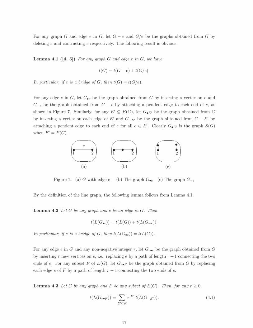
For any edge e in G, let G•e be the graph obtained from G by inserting a vertex on e and
G−e be the graph obtained from G − e by attaching a pendent edge to each end of e, as
shown in Figure 7. Similarly, for any E′ ⊆ E(G), let G•E′ be the graph obtained from G
by inserting a vertex on each edge of E′ and G−E′ be the graph obtained from G − E′ by
attaching a pendent edge to each end of e for all e ∈ E′. Clearly G•E′ is the graph S(G)
when E′ = E(G).✬
✫
✩
✪
✬
✫
✩
✪
✬
✫
✩
✪t t tt t tt t te
1 1 12 2 2
(a) (b) (c)
Figure 7: (a) G with edge e (b) The graph G•e (c) The graph G−e
By the definition of the line graph, the following lemma follows from Lemma 4.1.
Lemma 4.2 Let G be any graph and e be an edge in G. Then
t(L(G•e)) = t(L(G)) + t(L(G−e)).
In particular, if e is a bridge of G, then t(L(G•e)) = t(L(G)).
For any edge e in G and any non-negative integer r, let Gr•e be the graph obtained from G
by inserting r new vertices on e, i.e., replacing e by a path of length r+1 connecting the two
ends of e. For any subset F of E(G), let Gr•F be the graph obtained from G by replacing
each edge e of F by a path of length r + 1 connecting the two ends of e.
Lemma 4.3 Let G be any graph and F be any subset of E(G). Then, for any r ≥ 0,
t(L(Gr•F )) =∑
E′⊆F
r|E′|t(L(G−E′)). (4.1)
17

Proof. Note that for any two vertices u, v in a graph H, if NH(u) = {v} and dH(v) = 2,
then t(L(H)) = t(L(H − u)). Thus, for any edge e of G and any positive integer r, by
Lemma 4.2, we have
t(L(Gr•e)) = t(L(G(r−1)•e)) + t(L(G−e)), (4.2)
where G0•e is G. Applying (4.2) repeatedly deduces that
t(L(Gr•e)) = t(L(G)) + rt(L(G−e)). (4.3)
Note that (4.1) is obvious for F = ∅ or r = 0. Now assume that e ∈ F and r ≥ 1. By
induction, we have
t(L(Gr•F−{e})) =∑
E′⊆F−{e}
r|E′|t(L(G−E′)). (4.4)
By (4.3), we have
t(L(Gr•F )) = t(L(Gr•F−{e})) + rt(L((Gr•F−{e})−e)). (4.5)
Thus (4.1) follows immediately from (4.4). ✷
We are now ready to prove Theorem 1.1 for the case r ≥ 1.
Proof of Theorem 1.1 for r ≥ 1: Assume that r ≥ 1. By Lemma 4.3, we have
t(L(Sr(G))) =∑
E′⊆E(G)
r|E′|t(L(G−E′)). (4.6)
The above summation needs only to take those subsets E′ of E(G) with t(L(G−E′)) > 0 (i.e.
G−E′ is connected). Now let E′ be any fixed subset of E(G) such that G−E′ is connected
and let H denote G−E′ . By Theorem 1.1 for r = 0 (i.e., (1.9)),
t(L(G−E′)) =∑
T ′∈T (H)
∑
g∈Γ(E(H)−E(T ′))
∏
v∈V (H)
dH(v)dH (v)−2−|g−1(v)|. (4.7)
Observe that V (G) ⊆ V (H). For any v ∈ V (H), if v ∈ V (G), then dH(v) = dG(v); otherwise,
dH(v) = 1. Thus
∏
v∈V (H)
dH(v)dH (v)−2−|g−1(v)| =∏
v∈V (G)
dG(v)dG(v)−2−|g−1(v)|. (4.8)
For each T ′ ∈ T (H), T ′ contains all pendent edges in H and so T ′ corresponds to T , where
T = T ′[V (G)], which is a spanning tree of G−E′. Thus E(H)−E(T ′) = E(G−E′)−E(T )
and
t(L(G−E′)) =∑
T∈T (G−E′)
∑
g∈Γ(E(G−E′)−E(T ))
∏
v∈V (G)
dG(v)dG(v)−2−|g−1(v)|. (4.9)
By (4.6) and (4.9),
t(L(Sr(G))) =∑
E′∈E(G)
r|E′|
∑
T∈T (G−E′)
∑
g∈Γ(E(G−E′)−E(T ))
∏
v∈V (G)
dG(v)dG(v)−2−|g−1(v)|. (4.10)
18

By replacing E(G)− E′ − E(T ) by E′′, (4.10) implies that
t(L(Sr(G))) =∑
E′′⊆E(G)
∑
T ′∈T (G−E′′)
∑
g∈Γ(E′′)
r|E(G)|−|E′′|−|E(T ′)|∏
v∈V (G)
dG(v)dG(v)−2−|g−1(v)|
=∑
E′′⊆E(G)
r|E(G)|−|E′′|−|V (G)|+1t(G− E′′)∑
g∈Γ(E′′)
∏
v∈V (G)
dG(v)dG(v)−2−|g−1(v)|
=∑
E′′′⊆E(G)
r|E′′′|−|V (G)|+1t(G[E′′′])
∑
g∈Γ(E−E′′′)
∏
v∈V (G)
dG(v)dG(v)−2−|g−1(v)|.
Hence the case r ≥ 1 of Theorem 1.1 holds. ✷
5 Proof of Conjecture 1.1
Now we turn back to those connected graphs G mentioned in Conjecture 1.1 and apply the
following result and Theorem 1.1 to deduce a relation between t(L(Sr(G))) and t(G). The
case r = 1 of this relation is exactly the conclusion of Conjecture 1.1.
Lemma 5.1 Let H be any connected graph of order n and size m. For any integer i with
0 ≤ i ≤ m− n+ 1, we have
(m− n+ 1
i
)
t(H) =∑
E′⊆E(H)
|E′|=i
t(H − E′).
Proof. We prove this result by providing two different methods to determining the size of
the following set:
Θ = {(T,E′) : T is a spanning tree of H and E′ ⊆ E(H)− E(T ) with |E′| = i}.
Note that for each spanning tree T of H, as |E(H)| = m and |E(T )| = n− 1, the number of
subsets E′ of E(H)−E(T ) with |E′| = i is(m−n+1
i
). On the other hand, for each E′ ⊆ E(H)
with |E′| = i, there are exactly t(H−E′) spanning trees T of G such that E′ ⊆ E(H)−E(T ).
Thus the result holds. ✷
We now deduce the following consequence of Theorem 1.1 for those connected graphs G
mentioned in Conjecture 1.1.
Corollary 5.1 Let G be a connected graph of order n+ s and size m+ s in which s vertices
are of degree 1 and all others are of degree k, where k ≥ 2. Then, for any r ≥ 0,
t(L(Sr(G))) = km+s−n−1(rk + 2)m−n+1t(G).
19

Proof. For any E′ ⊆ E(G) with t(G[E′]) 6= 0, E′ contains every bridge of G, and so
d(ue) = d(ve) = k for all e ∈ E(G)− E′. By Theorem 1.1, we have
t(L(Sr(G))) = (kk−2)n∑
E′⊆E(G)
t(G[E′])r|E′|−(n+s)+1(2k−1)(m+s)−|E′|
= (kk−2)nr−(n+s)+1(2k−1)(m+s)∑
E′⊆E(G)
t(G[E′])r|E′|(2k−1)−|E′|
= (kk−2)nr−(n+s)+1(2k−1)(m+s)∑
E′′⊆E(G)
t(G− E′′)r|E(G)|−|E′′|(2k−1)|E′′|−|E(G)|
= (kk−2)nr−(n+s)+1(2k−1)(m+s)m−n+1∑
j=0
rm+s−j(2k−1)j−m−s∑
E′′⊆E(G)
|E′′|=j
t(G−E′′)
= (kk−2)nm−n+1∑
j=0
rm−n+1−j(2k−1)j(m− n+ 1
j
)
t(G) (by Lemma 5.1)
= (kk−2)n(r + 2k−1)m−n+1t(G)
= kn(k−2)−(m−n+1)(kr + 2)m−n+1t(G)
= km+s−n−1(kr + 2)m−n+1t(G),
where the last expression follows from the equality 2(m+ s) = kn+ s by the given conditions
on G. Hence the result is obtained. ✷
Notice that (1.3) is the special case of Corollary 5.1 for r = 0 while the conclusion of Con-
jecture 1.1 is the special case of Corollary 5.1 for r = 1.
We end this section with the the following result on some special bipartite graphs, which can
be obtained by applying Lemma 5.1 and the case r = 0 of Theorem 1.1.
Corollary 5.2 Let G = (A,B;E) be a connected bipartite graph of order n and size m such
that d(x) ∈ {1, a} for all x ∈ A and d(y) ∈ {1, b} for all y ∈ B, where a ≥ 2 and b ≥ 2. Then
t(L(G)) = a(a−2)n1b(b−2)n2(a−1 + b−1)m−n+1t(G),
where n1 is the number of vertices x in A with d(x) = a and n2 is the number of vertices y
in B with d(y) = b.
The result of Corollary 5.2 in the case that G is an (a, b)-semiregular bipartite graph was
originally due to Cvetkovic (see Theorem 3.9 in [13], §5.2 of [15], or [17]).
Acknowledgement. The authors wish to thank the referees for their very helpful suggestions.
20
References
[1] M. Aigner and G. Ziegler, Proofs from The Book, Fourth edition. Springer-Verlag, Berlin,
2010.
[2] A. Berget, A. Manion, M. Maxwell, A. Potechin, V. Reiner, The critical group of a line
graph, Ann. Comb. 16 (2012), 449-488.
[3] H. Bidkhori and S. Kishore, Counting spanning trees of a directed line graph, arXiv:
0910.3442v1.
[4] N. L. Biggs, Algebraic Graph Theory, 2nd edn, Cambridge, Cambridge University Press,
1993.
[5] J. A. Bondy and U. S. R. Murty, Graph Theory with Applications, American Elsevier,
New York, 1976.
[6] H. Y. Chen, F. J. Zhang, The critical group of a clique-inserted graph, Discrete Math.
319 (2014), 24-32.
[7] D.Cvetkovic, M.Doob, H.Sachs, Spectra of Graphs. Theory and Application, Pure Appl.
Math.,vol. 87, Academic Press,Inc. [Harcourt Brace Jovanovich, Publishers], New York,
London,1980.
[8] A.K.Kelmans, On properties of the characteristic polynomial of a graph, in:Kibernetiku
Na Sluzbu Kom., vol.4, Gosener-goizdat, Moscow, 1967, pp.27-47(in Russian).
[9] D.E. Knuth. Oriented subtrees of an arc digraph, J. of Combin. Theory 3 (1967), 309-
314.
[10] L. Levine, Sandpile groups and spanning trees of directed line graphs, J. of Combin.
Theory Ser. A 118 (2011), 350-364.
[11] L. Lovasz, Combinatorial Problems and Exercises, North-Holland, Amsterdam (1979).
[12] L. Lovasz, M.D. Plummer, Matching Theory, Ann. Discrete Math. 29, North-Holland,
Amsterdam, 1986.
[13] I.G. Macdonald, Symmetric functions and Hall polynomials, 2nd edition. Oxford Math-
ematical Monographs. Oxford Science Publications. The Clarendon Press, Oxford Uni-
versity Press, New York, 1995.
[14] W. Mader, Minimale n-fach kantenzusammenhangende Graphen, Math. Ann. 191
(1971), 21-28.
21

[15] B. Mohar, The Laplacian Spectrum of Graphs, Graph Theory, Combinatorics, and Ap-
plications 2 Ed. by Y. Alavi, G. Chartrand, O. R. Oellermann, A. J. Schwenk. Wiley,
1991, 871-898.
[16] D. Perkinson, N. Salter, T. Y. Xu, A note on the critical group of a line graph, Electron.
J. Combin. 18 (2011), #P124.
[17] I. Sato, Zeta functions and complexities of a semiregular bipartite graph and its line
graph, Discrete Math. 307 (2007), 237-245.
[18] T. Shirai, The spectrum of infinite regular line graphs, Trans. Amer. Math. Soc. 352
(2000), no. 1, 115-132.
[19] E.B.Vahovskii, On the characteristic numbers of incidence matrices for non-singular
graphs, Sibirsk. Mat. Zh. 6 (1965), 44-49 (in Russian).
[20] Weigen Yan, On the number of spanning trees of some irregular line graphs, J. Combin.
Theory Ser. A 120 (2013), 1642-1648.
[21] F.J.Zhang, Y.-C.Chen, Z.B.Chen, Clique-inserted-graphs and spectral dynamics of
clique-inserting, J. Math. Anal. Appl. 349 (2009), 211-225.
[22] Z. H. Zhang, Some physical and chemical indices of clique-inserted lattices, Journal of
Statistical Mechanics: Theory and Experiment, doi:10.1088/1742-5468/2013/10/P10004.
22
Top Related
Copyright © 2022 FDOKUMEN

