Download - Exploiting Long-Term Connectivity and Visual Motion in CRF-Based Multi-Person Tracking

3040 IEEE TRANSACTIONS ON IMAGE PROCESSING, VOL. 23, NO. 7, JULY 2014

Exploiting Long-Term Connectivity and VisualMotion in CRF-Based Multi-Person Tracking

Alexandre Heili, Student Member, IEEE, Adolfo López-Méndez, and Jean-Marc Odobez, Member, IEEE

Abstract— We present a conditional random field approach totracking-by-detection in which we model pairwise factors linkingpairs of detections and their hidden labels, as well as higherorder potentials defined in terms of label costs. To the contraryof previous papers, our method considers long-term connectivitybetween pairs of detections and models similarities as well asdissimilarities between them, based on position, color, and asnovelty, visual motion cues. We introduce a set of feature-specificconfidence scores, which aim at weighting feature contributionsaccording to their reliability. Pairwise potential parameters arethen learned in an unsupervised way from detections or fromtracklets. Label costs are defined so as to penalize the complexityof the labeling, based on prior knowledge about the scene likethe location of entry/exit zones. Experiments on PETS’09, TUD,CAVIAR, Parking Lot, and Town Center public data sets showthe validity of our approach, and similar or better performancethan recent state-of-the-art algorithms.

Index Terms— Multi-person tracking, tracking-by-detection,CRF, visual motion.

I. INTRODUCTION

AUTOMATED tracking of multiple people is a centralproblem in computer vision. It is particularly interesting

in video surveillance contexts, where tracking the positionof people over time might benefit tasks such as group andsocial behavior analysis, pose estimation or abnormalitydetection, to name a few. Nonetheless, multi-person trackingremains a challenging task, especially in single camerasettings, notably due to sensor noise, changing backgrounds,high crowding, occlusions, clutter and appearance similaritybetween individuals.

Tracking-by-detection methods have become increasinglypopular [8], [19], [37]. These methods aim at automaticallyassociating human detections across frames, such that eachset of associated detections univocally belongs to one indi-vidual in the scene. Compared to background modeling-based

Manuscript received August 14, 2013; revised January 9, 2014; acceptedApril 28, 2014. Date of publication May 14, 2014; date of current versionJune 9, 2014. This work was supported by the Integrated Project VANAHEIMunder Grant 248907 through the European Union under the 7th FrameworkProgram. The associate editor coordinating the review of this manuscript andapproving it for publication was Prof. Zhou Wang.

A. Heili and J.-M. Odobez are with École Polytechnique Fédérale deLausanne, Lausanne 1015, Switzerland, and also with Idiap Research Institute,Martigny 1920, Switzerland (e-mail: [email protected]; [email protected]).

A. López-Méndez is with Idiap Research Institute, Martigny 1920, Switzer-land (e-mail: [email protected]).

This paper has supplementary downloadable material available athttp://ieeexplore.ieee.org., provided by the author. The PDF file summarizesnotations used in the paper and contains some deeper details about their opti-mization algorithm. The document also presents more extensive experimentsshowing the benefit of the different paper contributions. The total size ofthe videos is 258 kB. Contact [email protected] for further questions aboutthis work.

Color versions of one or more of the figures in this paper are availableonline at http://ieeexplore.ieee.org.

Digital Object Identifier 10.1109/TIP.2014.2324292

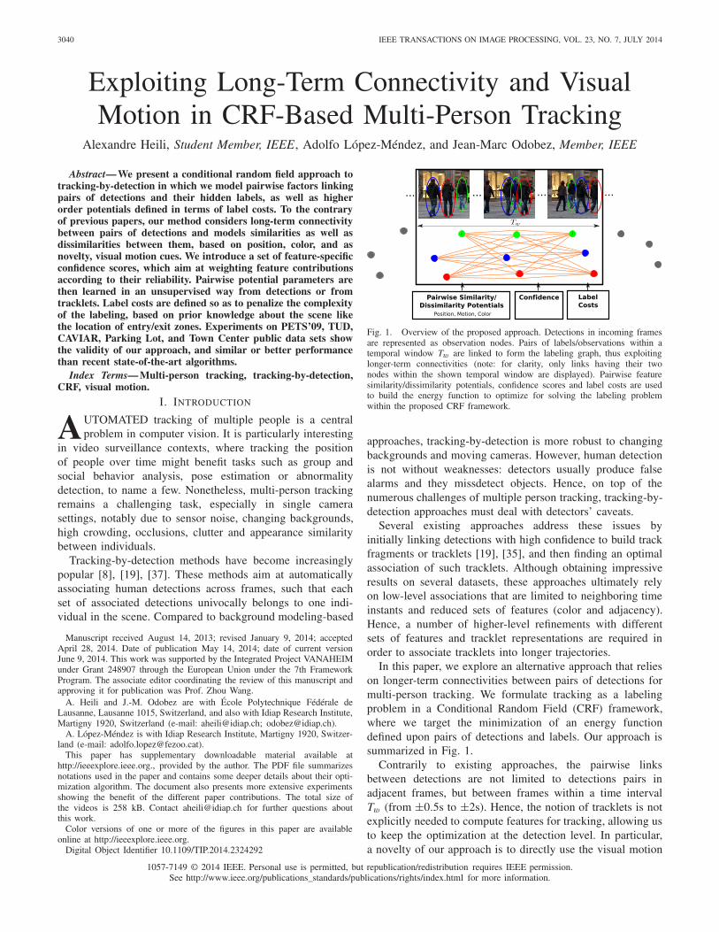
Fig. 1. Overview of the proposed approach. Detections in incoming framesare represented as observation nodes. Pairs of labels/observations within atemporal window Tw are linked to form the labeling graph, thus exploitinglonger-term connectivities (note: for clarity, only links having their twonodes within the shown temporal window are displayed). Pairwise featuresimilarity/dissimilarity potentials, confidence scores and label costs are usedto build the energy function to optimize for solving the labeling problemwithin the proposed CRF framework.

approaches, tracking-by-detection is more robust to changingbackgrounds and moving cameras. However, human detectionis not without weaknesses: detectors usually produce falsealarms and they missdetect objects. Hence, on top of thenumerous challenges of multiple person tracking, tracking-by-detection approaches must deal with detectors’ caveats.

Several existing approaches address these issues byinitially linking detections with high confidence to build trackfragments or tracklets [19], [35], and then finding an optimalassociation of such tracklets. Although obtaining impressiveresults on several datasets, these approaches ultimately relyon low-level associations that are limited to neighboring timeinstants and reduced sets of features (color and adjacency).Hence, a number of higher-level refinements with differentsets of features and tracklet representations are required inorder to associate tracklets into longer trajectories.

In this paper, we explore an alternative approach that relieson longer-term connectivities between pairs of detections formulti-person tracking. We formulate tracking as a labelingproblem in a Conditional Random Field (CRF) framework,where we target the minimization of an energy functiondefined upon pairs of detections and labels. Our approach issummarized in Fig. 1.

Contrarily to existing approaches, the pairwise linksbetween detections are not limited to detections pairs inadjacent frames, but between frames within a time intervalTw (from ±0.5s to ±2s). Hence, the notion of tracklets is notexplicitly needed to compute features for tracking, allowing usto keep the optimization at the detection level. In particular,a novelty of our approach is to directly use the visual motion

1057-7149 © 2014 IEEE. Personal use is permitted, but republication/redistribution requires IEEE permission.See http://www.ieee.org/publications_standards/publications/rights/index.html for more information.

HEILI et al.: EXPLOITING LONG-TERM CONNECTIVITY AND VISUAL MOTION 3041

computed from the video sequence for data association. Thisavoids resorting to tracklet creation or cumbersome tracklethypothesizing and testing optimization to obtain discriminativemotion information.

Another differential trait of our method is the form of energypotentials, formulated here in terms of similarity and dissim-ilarity between pairs of detections. Moreover, the proposedpotentials depend not only on sets of features, but also onthe time interval between two detections. In this way, wemodel how discriminative a feature is given the observeddistance in the feature space and the time gap between pairs ofdetections, an important characteristic when considering long-term connectivity. Furthermore, to take into account not onlythe actual feature distance value but also its reliability, weexploit a set of confidence scores per feature to characterizehow trustable the pairwise distances are. For instance, visualcue distances are given a lower confidence whenever one ofthe detections is possibly occluded. These scores ultimatelyallow to re-weight the contribution of each feature basedon spatio-temporal cues, and to rely on the most reliablepairwise links for labeling. This is important near occlusionsituations, where thanks to long-term connectivity, the labelingcan count on cleaner detections just before or after occlusionto propagate labels directly to the noisier detections obtainedduring occlusion instead of through adjacent drift-prone frame-to-frame pairwise links only.

One important advantage of our modeling scheme is that itallows to directly learn the pairwise potential parameters fromthe data in an unsupervised and incremental fashion. To thatend, we propose a criterion to first collect relevant detectionpairs to measure their similarity/dissimilarity statistics andlearn model parameters that are sensitive to the time intervalbetween detection pairs. Then, at a successive optimizationround, we can leverage on intermediate track information togather more reliable statistics and exploit them to estimateaccurate model parameters.

Finally, compared to some existing CRF approaches fortracking [17], [35], [37] a novel aspect of our framework isthat the energy function includes higher order terms in theform of label costs. The aim of such label costs is to modelpriors on label fields. In our tracking framework, this translatesinto penalizing the complexity of the labeling, mostly basedon the fact that sufficiently long tracks should start and endin specific areas of the scenario. We are interested in staticcamera settings, in which scene-specific maps can be definedfor that purpose.

To summarize, the paper addresses the multi-person trackingproblem within a tracking-by-detection approach and makescontributions in the following directions (see also Fig. 1):

1) A CRF framework formulated in terms of similar-ity/dissimilarity pairwise factors between detections andadditional higher-order potentials defined in terms of labelcosts. Differently from existing CRF frameworks, ourmethod considers long-term connectivity between pairs ofdetections. Note however that long-term temporal connec-tivity alone is generally not sufficient to guarantee goodresults, and needs to be exploited in conjunction withthe other contributions described below: visual motion,

confidence weights, time-sensitive parameters with unsu-pervised learning from tracklets.

2) A novel potential based on visual motion features. Visualmotion allows incorporating motion cues at the bottomassociation level, i.e., the detection level, rather thanthrough tracklet hypothesizing.

3) A set of confidence scores for each feature-based poten-tial and pair of detections. The proposed confidencescores model the reliability of the feature consideringspatio-temporal reasoning such as occlusions betweendetections.

4) Thanks to the similarity/dissimilarity formulation, theparameters defining the pairwise factors can be learned inan unsupervised fashion from detections or from tracklets,leading to accurate time-interval dependent factor terms.

Experiments conducted on standard public datasets show thebenefit of the different modeling contributions. They demon-strate that our optimization conducted at the detection nodelevel but relying on longer time window association leads tocompetitive performance compared to recent state-of-the artmethods.

The paper is structured as follows. Section II describesrelated work. The CRF framework is formulated in Section III.Pairwise potentials with associated confidence scores aredetailed in Section IV whereas label costs are described inSection V. Unsupervised parameter learning is explained inSection VI. Section VII describes the optimization methodol-ogy. Finally, experimental results are presented in Section VIII.

II. RELATED WORK

Tracking-by-detection methods have become increasinglypopular in the vision community. To the contrary of generativemethods [39], detection-based trackers use a discriminativeclassifier to assess the presence of an object in a scene,which is generally more robust, as state-of-the-art detectorsgive very good performance at detecting humans [13], [15].The detector’s output is used to generate target hypothesesin each frame, which then have to be transitively linked toform trajectories with consistent identity labels. Tracking-by-detection can therefore be formulated as a data associationproblem, which generally relies on affinity models betweendetections in successive frames based on motion constraintsand intrinsic object descriptors such as color [40].

The association problem is addressed by some approacheson a multi-frame basis [3], [28], [34]. Dependencies are oftenmodeled using graphs, and the optimization problem thenconsists in finding the best paths between all the detectionsin separate frames. The process can be applied on potentiallylarge time windows, so as to overcome the sparsity in thedetection sets induced by missed detections and also to dealwith false alarms, but the complexity of the optimizationincreases rapidly. Moreover, due to the temporal locality ofassociation considered in this context, tracking-by-detectiontechniques can perform poorly in presence of long-term occlu-sions, i.e. many successive missed detections.

Alternatively, to reduce the computation and to progres-sively increase the temporal range for correspondences, hier-archical approaches can be considered, in which low-level


tracklets are first generated and then merged at a higher-level. For instance, in [19], the lower level associates pairsof detections in adjacent frames based on their similarity inposition, size and appearance. The resulting tracklets are thenfed into a Maximum A Posteriori (MAP) association problemsolved by the Hungarian algorithm, and further refined at ahigher level to model scene exits and occluders. As thereare fewer tracklets than detections, the complexity of theoptimization is reduced, but any wrong association made at thelow-level is then propagated to the next hierarchy level. Thishierarchical association is also followed in the CRF modelspresented in [35] and [37]. The motivation of the CRF frame-work is to introduce pairwise potentials between tracklets,such that pairs of difficult tracklets can be better distinguished.While [22] and [36] make emphasis on learning discriminativeappearance models for tracklets, they both follow the hierar-chical association of [19]. Similarly, Bak et al. [5] proposed atwo-level association algorithm where tracklets are linked byusing discriminative analysis on a Riemannian manifold. Thedescribed methods perform bottom level associations betweenpairs of detections in consecutive frames, relying on a subset offeatures (motion information is not used at the bottom level).This limitation can be critical since early errors are propagatedto higher levels of the hierarchy.

A different approach to hierarchical association of detec-tions is presented in [41]. To generate the first level tracklets,detections within predefined short time windows are linked,thus breaking the frame adjacency constraint of previouslydescribed methods. Then, tracklet association between con-secutive windows is performed. At both levels, the sameoptimization framework is employed. The objective functionrelies on a motion model where all pairs of detections withinthe tracklet contribute to build a motion estimate which can beused with a constant speed assumption to compute a predictionerror. Additionally, a virtual detection generation approach isproposed in order to tackle occlusions.

Alternatively, some authors focus on global methods thataim at alleviating these short temporality limitations. Theyusually consider the whole span of the sequence, which canbe a problem if online processing is required. In [42], theauthors use a similar MAP formulation as in [19] but embedit in a network framework where min-cost flow algorithmcan be applied. The authors of [8] formulate the problemas finding the flow of humans on a discrete grid space thatminimizes the cost of going through the detections, which areobtained by fusing the foreground information from severalcamera views. In [30], the authors extend their method byadding global appearance constraints. Impressive results areobtained, but only results in indoor scenarios are shown,where relatively clean detections from multiview backgroundsubtraction images are used. Furthermore, in many trackingscenarios, multiple synchronized and calibrated cameras arenot available.

Labeling detections with identity can also be done jointlywith finding smooth trajectories that best explain the data.The method proposed in [4] tackles the problem by alter-nating between discrete data association and continuous tra-jectory estimation using global costs. This method relies

solely on trajectories and does not involve appearance ofobjects.

Some multi-person tracking algorithms focus on contextlearning and model adaptation in order to address possiblelimitations of pre-learned affinity models. Context modelsproposed in [38] and [32] rely on the availability of sufficienttraining data. If such data cannot be acquired, one can alter-natively adapt tracking models by using local crowd densityestimations [29]. Similarly, [31] propose a tracklet adaptationapproach based on the variance of the observed features alonga path. In [24], contextual cues such as target births and clutterintensities are incrementally learned using tracker feedback.

Different from the above, we benefit from important tem-poral context by connecting detection pairs not only betweenadjacent frames, but between frames within a long timeinterval. Not only we differentiate from [41] in that we exploitlonger-term connectivities between detections, but also inthat our method is built entirely on pairwise links betweendetections, allowing us to re-label detections at any iterationof the algorithm. Since the notion of tracklet is not explicitlyused in the proposed framework, we use motion informationby introducing a novel feature based on visual motion. Fur-thermore, to the contrary of most existing methods above, ourapproach does not only optimize the label field on a similarityhypothesis basis, but also relies on a dissimilarity informationto assess the labeling. By contrasting the two hypotheses foreach detection pair, the model is more robust to assess theappropriateness of a given association. Apart from the largerconnectivity between pairs of detections, our CRF frameworkdiffers from [35] and [37] in that we consider confidencescores for the features, as well as higher order potentials inthe form of label costs. Confidence scores can be regarded as acontext adaptation approach where, differently from methodssuch as [31], we do not rely on tracklets but on the positionof detections on a per-frame basis.

III. CRF TRACKING FRAMEWORK

This Section introduces the main elements of our trackingframework. We start by introducing our data representation,and then present how we formulate our tracking problem.A list of all symbols used in the manuscript, along with theirbrief definition and where they are introduced in the paper isgiven in the supplementary material.

A. Data Representation

Let us define the set of detections of a video sequenceas R = {ri }i=1:Nr , where Nr is the total number of detec-tions. The features we choose to represent our detections arearticulated around 3 cues: position, motion and color. Moreprecisely, each detection is defined as

ri = (ti , xi , vi , {hbi }b∈P ) (1)

which comprises the following features:

• ti denotes the time instant at which the detection occurs;• xi denotes the 2D image or ground-plane position

depending on the availability of calibration information;


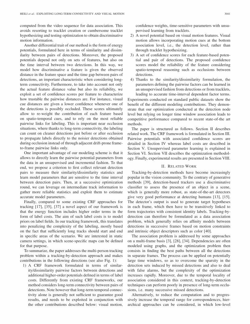
Fig. 2. Factor graph illustration of our Conditional Random Field model.

• vi denotes the 2D image plane visual motion computedfrom the video sequence;

• hbi with b ∈ P = {whole, head, torso, legs} denotes a set

of multi-resolution color histograms extracted from a setP of body parts.

Note that, in contrast to existing approaches, each detectionhas an associated motion vector vi , which is independentof the label field, i.e., motion is not derived from trackletsbut from detections. In our case, a robust estimation of thismotion is conducted by performing a weighted average of thedisplacement estimated at several body part patches resultingfrom a part-based human detector, where the weight of eachdisplacement vector indicates the motion reliability based onthe matching distance and how uniform the patch is. For thecolor descriptors, we define parts that represent the wholedetection region as well as three different spatial regions (head,torso, legs) to take advantage of both a holistic representationand heuristically defined body parts. Further implementationdetails are given in Section VIII-B.

B. Problem Formulation

We formulate multi-object tracking as a detection labelingproblem, in which we seek for the optimal label field L ={li }i=1:Nr , where li denotes the label of detection ri , so thatdetections within a same track should be assigned the samelabel. Labels can take their values in N as we do not know inadvance the number of objects in the scene.

To solve this labeling task, we rely on a CRF formulation.Assuming the graphical model and factor graph shown inFig. 2, we model the posterior probability of the label fieldgiven all the observations as follows:

p(L|R, λ) = 1

Z(R)�Pair (L, R,W, λ)�L (L) (2)

∝⎛⎝ ∏

(i, j )∈I

N f∏k=1

�k(li , l j , ri , r j , wki j , λ

k)

⎞⎠�L(L) (3)

where I denotes the set of connected detection pairs, for eachdetection pair we introduce N f factor terms �k to accountfor different pairwise feature similarity/dissimilarity measure-ments, λ = {λk} denotes the set of parameters associated witheach of these factors, and W = {wk

i j } with wki j ∈ [0, 1] denotes

the set of confidence scores associated with each featureand detection pairs. In contrast to [18] that only consideredpairwise terms, the above formulation incorporates a prior �L

over label fields in terms of higher-order potentials. This prior

acts as regularizers penalizing complex solutions, and will bedetailed in Section V.

C. Factor Modeling

The factors �k are modeled using a long-term, two-hypothesis, time-interval dependent and confident pairwiseapproach, as explained below. Firstly, we limit the number ofdetection pairs (ri , r j ) to be considered by imposing a long-term connectivity constraint:

I = {(i, j) / 1 ≤ �i j = |t j − ti | ≤ Tw}. (4)

where Tw is our long term window size. Secondly, for eachfactor term, a feature function fk(ri , r j ) is defined that com-putes a distance measure between detection characteristics.Then, the corresponding CRF pairwise factor is defined as:

�k(li , l j , ri , r j , wki j , λ

k)�= p( fk(ri , r j )|H (li, l j ), λ

k�i j

)wk

i j .

(5)

where the symbol�= means by definition. This factor depends

on the distribution p( fk |H, λk�) of the feature distance fk

under two different hypotheses corresponding to whether thelabels are the same or not, that is:

H (li , l j ) ={

H0 if li �= l j

H1 if li = l j(6)

Furthermore, the feature distribution under the two hypothesesis time-interval sensitive, in the sense that we define such adistribution for each time interval � that can separate twodetections. This allows to take into account the evolution ofthe feature according to this time parameter. In the model, thedependency is introduced thanks to the use of different sets ofparameters λk

� for each interval �.Finally, the factor �k defined by Eq. 5 accounts for the

confidence wki j we have between detection pairs by powering

the feature distribution with wki j . Intuitively, lower confidence

values will flatten the distribution of a feature leading to lessdiscriminative potential, lowering the factor difference underthe two hypotheses. At the limit, if wk

i j = 0, the factor of agiven feature distance will be identical (equal to one) underthe two hypotheses.

D. Equivalent Energy Minimization

Our goal is to optimize the probability defined by Eq. 3.Given our factor definition (Eq. 5) and since the confi-dence scores are independent of the hypothesis H (li , l j ),we can divide the expression of Eq. 3 by Cst =∏

(i, j )∈I∏

k p( fk(ri , r j )|H0, λk�i j

)wk

i j . By further taking thenegative logarithm of the resulting expression, the maximiza-tion of Eq. 3 can be equivalently conducted by minimizing thefollowing energy:

U(L) =⎛⎝∑

(i, j )

N f∑k=1

wki j βk

i j δ(li − l j )

⎞⎠ + �(L) (7)

where δ(.) denotes the Kronecker function (δ(a) = 1 if a = 0,δ(a) = 0 otherwise), the Potts coefficients for each pairwise


link and each feature distance are defined as:

βki j = log

[p( fk(ri , r j )|H0, λ

k�i j

)

p( fk(ri , r j )|H1, λk�i j

)

], (8)

and the term �(L) = − log �L(L) represents the label cost.As can be seen, for each feature, the Potts coefficients are

defined by the loglikelihood ratio of the feature distance of adetection pair under the two hypotheses. Since in the energyof Eq. 7, the terms for pairs having different labels (li �= l j )vanish and only those for which li = l j remain, the Pottscoefficient can be seen as “costs” for associating a detectionpair within the same track. When βk

i j < 0, the more negativethis coefficient will be, the more likely the pair of detectionsshould be associated, so as to minimize the energy in Eq. 7.Reversely, when βk

i j > 0, the more positive this coefficientwill be, the more likely the pair of detections should notbe associated, so as to minimize the energy in Eq. 7. Whenβk

i j = 0, there is no preference for associating or not the pairs.In the following Section, the specific features, factor models

and confidence scores will be defined and illustrated. The labelcost term �(L) will be defined in Section V.

IV. SIMILARITY/DISSIMILARITY CONFIDENT

FACTOR MODELING

The previous Section introduced our general modelingapproach. In this Section, we specify more precisely thedifferent pairwise feature functions fk that we have consideredalong with their associated distributions and the parametersthat characterize them. In practice, we used N f = 7 featurefunctions constructed around three cues: position, motion andcolor. Their definitions are provided in Subsections IV-A, IV-Band IV-C, while IV-D summarizes the model parameters thatspecify them and that will be learned automatically. In asecond stage (Subsection IV-E) we will present the pairwiseconfidence scores wk

i, j that are used to weight the contributionof each factor term of a detection pair in the overall energy.Note that the focus of this Section is on the design of thesimilarity distributions, and that parameter learning will bedescribed later in Section VI.

A. Position Cue Similarity Distributions

The position feature is defined for k = 1 as f1(ri , r j ) =xi − x j . We assume that its probability follows a Gaussiandistribution with 0 mean and whose covariance depends onthe two label hypotheses H0 or H1 and also on the time gap�i j = |ti − t j | between the detection pairs:

p( f1(ri , r j )= f |H (li, l j )= H, λ1)=N ( f ; 0,�H�i j

) (9)

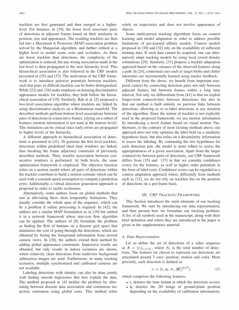
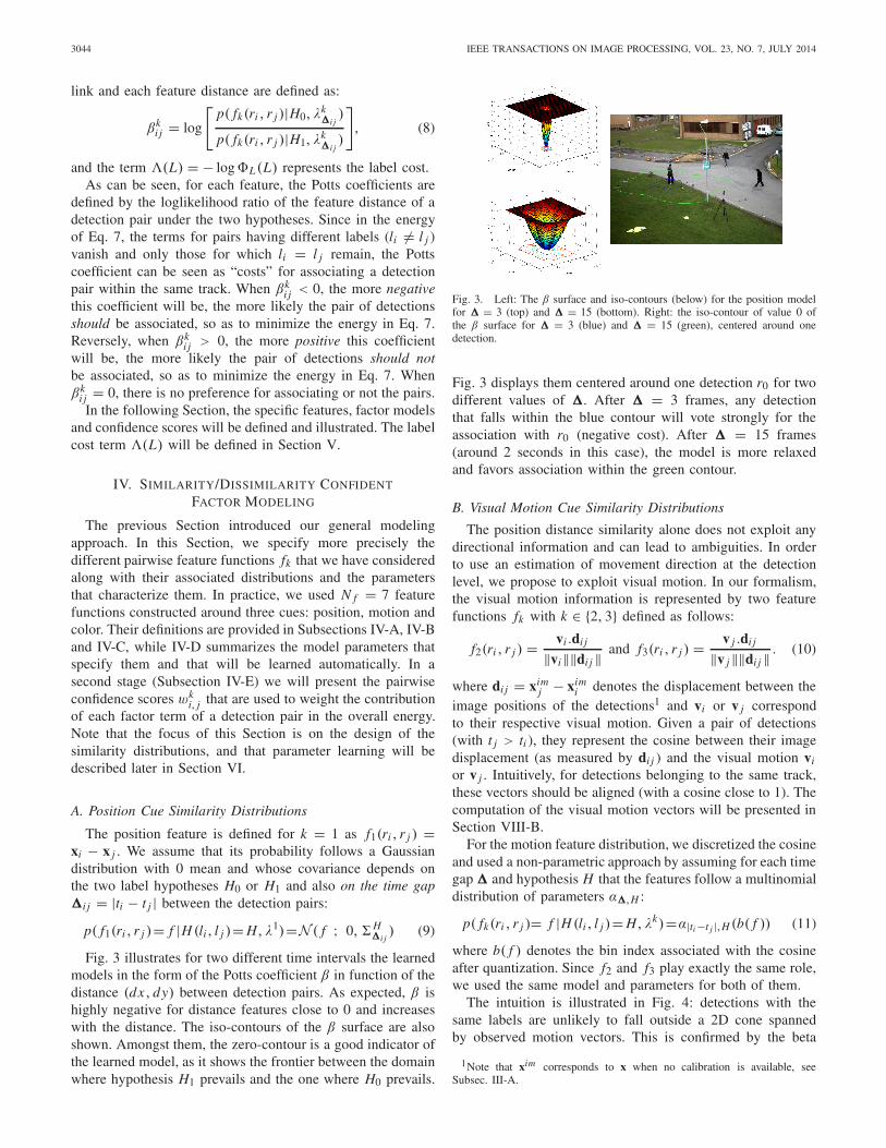
Fig. 3 illustrates for two different time intervals the learnedmodels in the form of the Potts coefficient β in function of thedistance (dx, dy) between detection pairs. As expected, β ishighly negative for distance features close to 0 and increaseswith the distance. The iso-contours of the β surface are alsoshown. Amongst them, the zero-contour is a good indicator ofthe learned model, as it shows the frontier between the domainwhere hypothesis H1 prevails and the one where H0 prevails.

Fig. 3. Left: The β surface and iso-contours (below) for the position modelfor � = 3 (top) and � = 15 (bottom). Right: the iso-contour of value 0 ofthe β surface for � = 3 (blue) and � = 15 (green), centered around onedetection.

Fig. 3 displays them centered around one detection r0 for twodifferent values of �. After � = 3 frames, any detectionthat falls within the blue contour will vote strongly for theassociation with r0 (negative cost). After � = 15 frames(around 2 seconds in this case), the model is more relaxedand favors association within the green contour.

B. Visual Motion Cue Similarity Distributions

The position distance similarity alone does not exploit anydirectional information and can lead to ambiguities. In orderto use an estimation of movement direction at the detectionlevel, we propose to exploit visual motion. In our formalism,the visual motion information is represented by two featurefunctions fk with k ∈ {2, 3} defined as follows:

f2(ri , r j ) = vi .di j

‖vi‖‖di j ‖ and f3(ri , r j ) = v j .di j

‖v j‖‖di j ‖ . (10)

where di j = ximj − xim

i denotes the displacement between theimage positions of the detections1 and vi or v j correspondto their respective visual motion. Given a pair of detections(with t j > ti ), they represent the cosine between their imagedisplacement (as measured by di j ) and the visual motion vi

or v j . Intuitively, for detections belonging to the same track,these vectors should be aligned (with a cosine close to 1). Thecomputation of the visual motion vectors will be presented inSection VIII-B.

For the motion feature distribution, we discretized the cosineand used a non-parametric approach by assuming for each timegap � and hypothesis H that the features follow a multinomialdistribution of parameters α�,H :

p( fk(ri , r j )= f |H (li , l j )= H, λk)=α|ti −t j |,H (b( f )) (11)

where b( f ) denotes the bin index associated with the cosineafter quantization. Since f2 and f3 play exactly the same role,we used the same model and parameters for both of them.

The intuition is illustrated in Fig. 4: detections with thesame labels are unlikely to fall outside a 2D cone spannedby observed motion vectors. This is confirmed by the beta

1Note that xim corresponds to x when no calibration is available, seeSubsec. III-A.


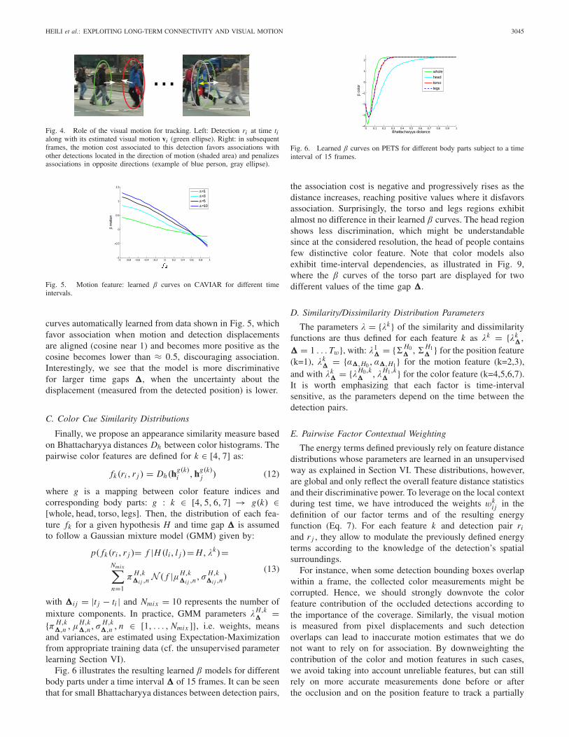
Fig. 4. Role of the visual motion for tracking. Left: Detection ri at time tialong with its estimated visual motion vi (green ellipse). Right: in subsequentframes, the motion cost associated to this detection favors associations withother detections located in the direction of motion (shaded area) and penalizesassociations in opposite directions (example of blue person, gray ellipse).

Fig. 5. Motion feature: learned β curves on CAVIAR for different timeintervals.

curves automatically learned from data shown in Fig. 5, whichfavor association when motion and detection displacementsare aligned (cosine near 1) and becomes more positive as thecosine becomes lower than ≈ 0.5, discouraging association.Interestingly, we see that the model is more discriminativefor larger time gaps �, when the uncertainty about thedisplacement (measured from the detected position) is lower.

C. Color Cue Similarity Distributions

Finally, we propose an appearance similarity measure basedon Bhattacharyya distances Dh between color histograms. Thepairwise color features are defined for k ∈ [4, 7] as:

fk(ri , r j ) = Dh(hg(k)i , hg(k)

j ) (12)

where g is a mapping between color feature indices andcorresponding body parts: g : k ∈ [4, 5, 6, 7] → g(k) ∈[whole, head, torso, legs]. Then, the distribution of each fea-ture fk for a given hypothesis H and time gap � is assumedto follow a Gaussian mixture model (GMM) given by:

p( fk(ri , r j )= f |H (li, l j )= H, λk)=Nmix∑n=1

π H,k�i j ,n

N ( f |μH,k�i j ,n

, σ H,k�i j ,n

)(13)

with �i j = |t j − ti | and Nmix = 10 represents the number ofmixture components. In practice, GMM parameters λH,k

� ={π H,k

�,n , μH,k�,n, σ H,k

�,n , n ∈ [1, . . . , Nmix ]}, i.e. weights, meansand variances, are estimated using Expectation-Maximizationfrom appropriate training data (cf. the unsupervised parameterlearning Section VI).

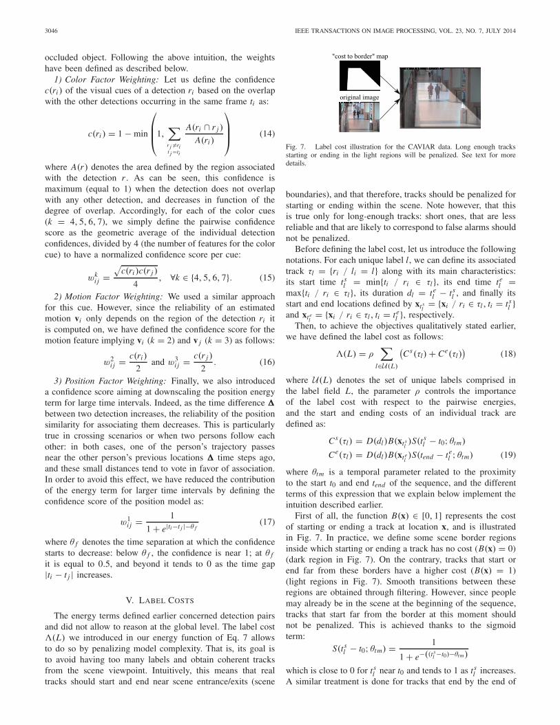
Fig. 6 illustrates the resulting learned β models for differentbody parts under a time interval � of 15 frames. It can be seenthat for small Bhattacharyya distances between detection pairs,

Fig. 6. Learned β curves on PETS for different body parts subject to a timeinterval of 15 frames.

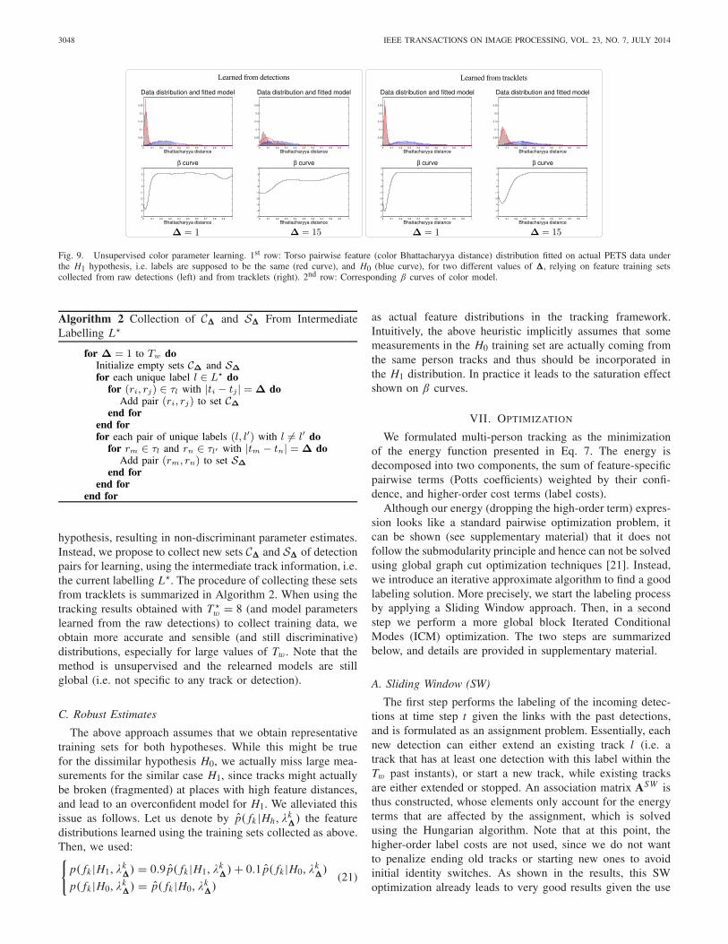
the association cost is negative and progressively rises as thedistance increases, reaching positive values where it disfavorsassociation. Surprisingly, the torso and legs regions exhibitalmost no difference in their learned β curves. The head regionshows less discrimination, which might be understandablesince at the considered resolution, the head of people containsfew distinctive color feature. Note that color models alsoexhibit time-interval dependencies, as illustrated in Fig. 9,where the β curves of the torso part are displayed for twodifferent values of the time gap �.

D. Similarity/Dissimilarity Distribution Parameters

The parameters λ = {λk} of the similarity and dissimilarityfunctions are thus defined for each feature k as λk = {λk

�,

� = 1 . . . Tw}, with: λ1� = {�H0

� ,�H1� } for the position feature

(k=1), λk� = {α�,H0 , α�,H1} for the motion feature (k=2,3),

and with λk� = {λH0,k

� , λH1,k� } for the color feature (k=4,5,6,7).

It is worth emphasizing that each factor is time-intervalsensitive, as the parameters depend on the time between thedetection pairs.

E. Pairwise Factor Contextual Weighting

The energy terms defined previously rely on feature distancedistributions whose parameters are learned in an unsupervisedway as explained in Section VI. These distributions, however,are global and only reflect the overall feature distance statisticsand their discriminative power. To leverage on the local contextduring test time, we have introduced the weights wk

i j in thedefinition of our factor terms and of the resulting energyfunction (Eq. 7). For each feature k and detection pair ri

and r j , they allow to modulate the previously defined energyterms according to the knowledge of the detection’s spatialsurroundings.

For instance, when some detection bounding boxes overlapwithin a frame, the collected color measurements might becorrupted. Hence, we should strongly downvote the colorfeature contribution of the occluded detections according tothe importance of the coverage. Similarly, the visual motionis measured from pixel displacements and such detectionoverlaps can lead to inaccurate motion estimates that we donot want to rely on for association. By downweighting thecontribution of the color and motion features in such cases,we avoid taking into account unreliable features, but can stillrely on more accurate measurements done before or afterthe occlusion and on the position feature to track a partially


occluded object. Following the above intuition, the weightshave been defined as described below.

1) Color Factor Weighting: Let us define the confidencec(ri ) of the visual cues of a detection ri based on the overlapwith the other detections occurring in the same frame ti as:

c(ri ) = 1 − min

⎛⎜⎜⎝1,

∑r j �=rit j =ti

A(ri ∩ r j )

A(ri )

⎞⎟⎟⎠ (14)

where A(r) denotes the area defined by the region associatedwith the detection r . As can be seen, this confidence ismaximum (equal to 1) when the detection does not overlapwith any other detection, and decreases in function of thedegree of overlap. Accordingly, for each of the color cues(k = 4, 5, 6, 7), we simply define the pairwise confidencescore as the geometric average of the individual detectionconfidences, divided by 4 (the number of features for the colorcue) to have a normalized confidence score per cue:

wki j =

√c(ri )c(r j )

4, ∀k ∈ {4, 5, 6, 7}. (15)

2) Motion Factor Weighting: We used a similar approachfor this cue. However, since the reliability of an estimatedmotion vi only depends on the region of the detection ri itis computed on, we have defined the confidence score for themotion feature implying vi (k = 2) and v j (k = 3) as follows:

w2i j = c(ri )

2and w3

i j = c(r j )

2. (16)

3) Position Factor Weighting: Finally, we also introduceda confidence score aiming at downscaling the position energyterm for large time intervals. Indeed, as the time difference �

between two detection increases, the reliability of the positionsimilarity for associating them decreases. This is particularlytrue in crossing scenarios or when two persons follow eachother: in both cases, one of the person’s trajectory passesnear the other person’s previous locations � time steps ago,and these small distances tend to vote in favor of association.In order to avoid this effect, we have reduced the contributionof the energy term for larger time intervals by defining theconfidence score of the position model as:

w1i j = 1

1 + e|ti−t j |−θ f(17)

where θ f denotes the time separation at which the confidencestarts to decrease: below θ f , the confidence is near 1; at θ f

it is equal to 0.5, and beyond it tends to 0 as the time gap|ti − t j | increases.

V. LABEL COSTS

The energy terms defined earlier concerned detection pairsand did not allow to reason at the global level. The label cost�(L) we introduced in our energy function of Eq. 7 allowsto do so by penalizing model complexity. That is, its goal isto avoid having too many labels and obtain coherent tracksfrom the scene viewpoint. Intuitively, this means that realtracks should start and end near scene entrance/exits (scene

Fig. 7. Label cost illustration for the CAVIAR data. Long enough tracksstarting or ending in the light regions will be penalized. See text for moredetails.

boundaries), and that therefore, tracks should be penalized forstarting or ending within the scene. Note however, that thisis true only for long-enough tracks: short ones, that are lessreliable and that are likely to correspond to false alarms shouldnot be penalized.

Before defining the label cost, let us introduce the followingnotations. For each unique label l, we can define its associatedtrack τl = {ri / li = l} along with its main characteristics:its start time ts

l = min{ti / ri ∈ τl}, its end time tel =

max{ti / ri ∈ τl}, its duration dl = tel − ts

l , and finally itsstart and end locations defined by xt s

l= {xi / ri ∈ τl , ti = ts

l }and xt e

l= {xi / ri ∈ τl , ti = te

l }, respectively.Then, to achieve the objectives qualitatively stated earlier,

we have defined the label cost as follows:

�(L) = ρ∑

l∈U(L)

(Cs(τl) + Ce(τl)

)(18)

where U(L) denotes the set of unique labels comprised inthe label field L, the parameter ρ controls the importanceof the label cost with respect to the pairwise energies,and the start and ending costs of an individual track aredefined as:

Cs(τl) = D(dl)B(xt sl)S(ts

l − t0; θtm)

Ce(τl) = D(dl)B(xt el)S(tend − te

l ; θtm) (19)

where θtm is a temporal parameter related to the proximityto the start t0 and end tend of the sequence, and the differentterms of this expression that we explain below implement theintuition described earlier.

First of all, the function B(x) ∈ [0, 1] represents the costof starting or ending a track at location x, and is illustratedin Fig. 7. In practice, we define some scene border regionsinside which starting or ending a track has no cost (B(x) = 0)(dark region in Fig. 7). On the contrary, tracks that start orend far from these borders have a higher cost (B(x) = 1)(light regions in Fig. 7). Smooth transitions between theseregions are obtained through filtering. However, since peoplemay already be in the scene at the beginning of the sequence,tracks that start far from the border at this moment shouldnot be penalized. This is achieved thanks to the sigmoidterm:

S(tsl − t0; θtm) = 1

1 + e−((t sl −t0)−θtm)

which is close to 0 for tsl near t0 and tends to 1 as ts

l increases.A similar treatment is done for tracks that end by the end of


the sequence, since people might still be in the scene at thatmoment.

Finally, since short tracks that are less reliable might bedue to false alarms, they should not be too much penalized toavoid encouraging their association. Thus the overall cost ismodulated according to the track duration:

D(dl) = min(dl , dmax) (20)

where dmax is a saturation value beyond which a track isconsidered long enough to be reliable, and all tracks arepenalized in the same way.

VI. UNSUPERVISED PARAMETER LEARNING

The appropriate setting of the model parameters is of crucialimportance for achieving good tracking results, but can bea tedious task. We remind that since distributions exhibitedtime dependencies, we have defined our models to be time-sensitive and feature-specific, which means that parametersneed to be defined for each feature and each time intervalup to Tw. Moreover, parameters also depend on the two-foldhypothesis H , so that ultimately, we have a large parameterspace size. In practice, one would like to avoid supervisedlearning, as this would require tedious track labeling for eachscene or camera.

In the following we propose an approach for learningthe factor parameter set in an unsupervised fashion. Moreprecisely, the first step is to learn model parameters by relyingdirectly on the raw detections within training videos of a givenscene. For convenience, we denote with a � superscript thenotations that apply to these initial models (for instance, thesemodels are learned up to T �

w). These models can be used fortracking on these training videos, and, provided we use a lowT �

w value, can lead to pure tracklets [17].Thus, in a second step, these tracklets corresponding to an

intermediate labelling L� can be conveniently used to refinemodel parameters and learn parameters for larger Tw values.The process could then be iterated (use new learned parametersfor tracking, then resulting tracklet for parameters learning),but experiments showed that in general no further gain can beachieved.

In this paper, since we consider rather short sequences fortesting, unsupervised learning is performed in batch modedirectly on the test sequence, i.e. the training set is the wholetest sequence, except for the CAVIAR dataset, in which weuse as training videos the set of 6 videos that are not used inthe test. The overall procedure of unsupervised batch learningand tracking is summarized in the block diagram of Fig. 8.More details are provided below.

A. Unsupervised Learning From Detections

Learning the model parameters λ can be done in a fullyunsupervised way using a sequence of detection outputs.

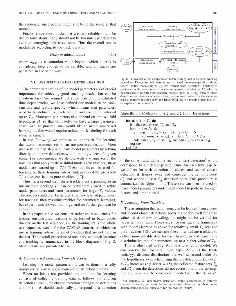
When no labels are provided, the intuition for learningconsists of collecting training data as follows: for a givendetection at time t , the closest detection amongst the detectionsat time t + � should statistically correspond to a detection

Fig. 8. Flowchart of the unsupervised batch learning and subsequent trackingprocedure. Detections and features are extracted on scene-specific trainingvideos. Initial models up to T �

w are learned from detections. Tracking isperformed with these models to obtain an intermediate labelling L�, which isin turn used to relearn more accurate models up to Tw > T �

w . Finally, givendetections and features of a test video, these refined models for the scene areused to perform tracking (SW and Block ICM are two tracking steps that willbe explained in Section VII).

Algorithm 1 Collection of C�� and S�

� From Detections

of the same track, while the second closest detection2 wouldcorrespond to a different person. Thus, for each time gap �,we collect for each detection its closest and second closestdetection � frames away and construct the set of closestC�

� and second closest S�� detection pairs. This procedure is

summarized in Algorithm 1. These sets can then be used tolearn model parameters under each model hypothesis for eachfeature and time interval.

B. Learning From Tracklets

The assumption that parameters can be learned from closestand second closest detections holds reasonably well for smallvalues of � or low crowding, but might not be verified forlarger temporal gaps. However, since our tracking frameworkwith models learned as above for relatively small Tw leads topure tracklets [18], we can use these intermediate tracklets tocollect more reliable data for each hypothesis and learn morediscriminative model parameters, up to a higher value of Tw.

This is illustrated in Fig. 9 for the torso color model. Wecan observe that for small time gaps (� = 1) the Bhat-tacharyya distance distributions are well separated under thetwo hypotheses, even when using the raw detections. However,as Tw increases (e.g. for � = 15), the collected feature sets C�

�and S�

� from the detections do not correspond to the assump-tion any more and become more blended w.r.t. the H1 or H0

2In principle, all non-closest detections would correspond to differentpersons. However, we used the second closest detection to obtain morediscriminative models, especially for the position feature.


Fig. 9. Unsupervised color parameter learning. 1st row: Torso pairwise feature (color Bhattacharyya distance) distribution fitted on actual PETS data underthe H1 hypothesis, i.e. labels are supposed to be the same (red curve), and H0 (blue curve), for two different values of �, relying on feature training setscollected from raw detections (left) and from tracklets (right). 2nd row: Corresponding β curves of color model.

Algorithm 2 Collection of C� and S� From IntermediateLabelling L�

hypothesis, resulting in non-discriminant parameter estimates.Instead, we propose to collect new sets C� and S� of detectionpairs for learning, using the intermediate track information, i.e.the current labelling L�. The procedure of collecting these setsfrom tracklets is summarized in Algorithm 2. When using thetracking results obtained with T �

w = 8 (and model parameterslearned from the raw detections) to collect training data, weobtain more accurate and sensible (and still discriminative)distributions, especially for large values of Tw . Note that themethod is unsupervised and the relearned models are stillglobal (i.e. not specific to any track or detection).

C. Robust Estimates

The above approach assumes that we obtain representativetraining sets for both hypotheses. While this might be truefor the dissimilar hypothesis H0, we actually miss large mea-surements for the similar case H1, since tracks might actuallybe broken (fragmented) at places with high feature distances,and lead to an overconfident model for H1. We alleviated thisissue as follows. Let us denote by p̂( fk |Hh, λ

k�) the feature

distributions learned using the training sets collected as above.Then, we used:{

p( fk |H1, λk�) = 0.9 p̂( fk |H1, λ

k�) + 0.1 p̂( fk |H0, λ

k�)

p( fk |H0, λk�) = p̂( fk |H0, λ

k�)

(21)

as actual feature distributions in the tracking framework.Intuitively, the above heuristic implicitly assumes that somemeasurements in the H0 training set are actually coming fromthe same person tracks and thus should be incorporated inthe H1 distribution. In practice it leads to the saturation effectshown on β curves.

VII. OPTIMIZATION

We formulated multi-person tracking as the minimizationof the energy function presented in Eq. 7. The energy isdecomposed into two components, the sum of feature-specificpairwise terms (Potts coefficients) weighted by their confi-dence, and higher-order cost terms (label costs).

Although our energy (dropping the high-order term) expres-sion looks like a standard pairwise optimization problem, itcan be shown (see supplementary material) that it does notfollow the submodularity principle and hence can not be solvedusing global graph cut optimization techniques [21]. Instead,we introduce an iterative approximate algorithm to find a goodlabeling solution. More precisely, we start the labeling processby applying a Sliding Window approach. Then, in a secondstep we perform a more global block Iterated ConditionalModes (ICM) optimization. The two steps are summarizedbelow, and details are provided in supplementary material.

A. Sliding Window (SW)

The first step performs the labeling of the incoming detec-tions at time step t given the links with the past detections,and is formulated as an assignment problem. Essentially, eachnew detection can either extend an existing track l (i.e. atrack that has at least one detection with this label within theTw past instants), or start a new track, while existing tracksare either extended or stopped. An association matrix ASW isthus constructed, whose elements only account for the energyterms that are affected by the assignment, which is solvedusing the Hungarian algorithm. Note that at this point, thehigher-order label costs are not used, since we do not wantto penalize ending old tracks or starting new ones to avoidinitial identity switches. As shown in the results, this SWoptimization already leads to very good results given the use


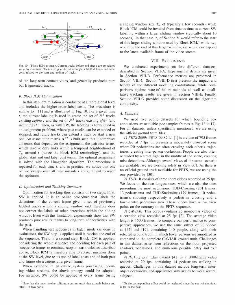
Fig. 10. Block ICM at time t . Current tracks before and after t are associatedso as to minimize block-wise β costs between pairs (dotted lines) and labelcosts related to the start and ending of tracks.

of the long-term connectivities, and generally produces purebut fragmented tracks.

B. Block ICM Optimization

In this step, optimization is conducted at a more global leveland includes the higher-order label costs. The procedure issimilar to [11] and is illustrated in Fig. 10. For a given timet , the current labeling is used to create the set of N B tracksexisting before t and the set of N A tracks existing after (andincluding) t .3 Then, as with SW, the labeling is formulated asan assignment problem, where past tracks can be extended orstopped, and future tracks can extend a track or start a newone. An association matrix AB I is built such that it comprisesall terms that depend on the assignment: the pairwise terms,which involve only links within a temporal neighborhood ofTw around t (hence the block ICM terminology), and theglobal start and end label cost terms. The optimal assignmentis solved with the Hungarian algorithm. The procedure isrepeated for each time t , and in practice, we notice that oneor two sweeps over all time instants t are sufficient to reachthe optimum.

C. Optimization and Tracking Summary

Optimization for tracking thus consists of two steps. First,SW is applied. It is an online procedure that labels thedetections of the current frame given a set of previouslylabeled tracks within a sliding window, end therefore doesnot correct the labels of other detections within the slidingwindow. Even with this limitation, experiments show that SWproduces pure results thanks to long-term connectivities withthe past.

When handling test sequences in batch mode (as done inevaluation), the SW step is applied until it reaches the end ofthe sequence. Then, in a second step, Block ICM is applied,considering the whole sequence and deciding for each pair ofsuccessive frames to continue, stop or start tracks, as describedabove. Block ICM is therefore able to correct mistakes doneat the SW level, due to its use of label costs and of both pastand future observations at a given frame.

When exploited in an online system processing incom-ing video streams, the above strategy could be adapted.For instance, SW could be applied at every frame (using

3Note that this may involve splitting a current track that extends before andafter t in two parts.

a sliding window size Tw of typically a few seconds), whileBlock ICM could be invoked from time to time to correct SWlabelling within a larger sliding window (typically about 10seconds). In that case, t0 of Section V would refer to the startof this larger sliding window used by Block ICM,4 while tend

would be the end of this larger window, i.e. would correspondto the latest available frame of the video stream.

VIII. EXPERIMENTS

We conducted experiments on five different datasets,described in Section VIII-A. Experimental details are givenin Section VIII-B. Performance metrics are presented inSection VIII-C. Section VIII-D first presents the impact andbenefit of the different modeling contributions, while com-parisons against state-of-the-art methods as well as quali-tative tracking results are given in Section VIII-E. Finally,Section VIII-G provides some discussion on the algorithmcomplexity.

A. Datasets

We used five public datasets for which bounding boxannotations are available (see samples frames in Fig. 13 to 17).For all datasets, unless specifically mentioned, we are usingthe official ground truth files.

1) PETS 2009: PETS’09 S2.L1 [1] is a video of 795 framesrecorded at 7 fps. It presents a moderately crowded scenewhere 20 pedestrians are often crossing each other’s trajec-tories, creating inter-person occlusions. People are also oftenoccluded by a street light in the middle of the scene, creatingmiss-detections. Although several views of the same scenarioare available, we are working solely in View 001. As there isno official ground truth available for PETS, we are using theone provided by [30].

2) TUD: It consists of three short videos recorded at 25 fps.We focus on the two longest ones, which are also the onespresenting the most occlusions: TUD-Crossing (201 frames,13 pedestrians) and TUD-Stadtmitte (179 frames, 10 pedes-trians), showing respectively a pedestrian crossing and atown-centre pedestrian area. These videos have a low viewpoint, on the contrary to the PETS sequence.

3) CAVIAR: This corpus contains 26 monocular videos ofa corridor view recorded at 25 fps [2]. The average videolength is 1500 frames. To compare our performance to com-petitive approaches, we use the same subset of 20 videosas [42] and [19], containing 140 people, along with theirselected ground truth, in which fewer persons are annotated ascompared to the complete CAVIAR ground truth. Challengesin this dataset arise from reflections on the floor, projectedshadows, occlusions, and numerous possible entry and exitpoints.

4) Parking Lot: This dataset [41] is a 1000-frame videorecorded at 29 fps, containing 14 pedestrians walking inqueues. Challenges in this dataset include long-term inter-object occlusions, and appearance similarities between severalsubjects.

4Or the corresponding effect could be neglected since the start of the videois far in the past.


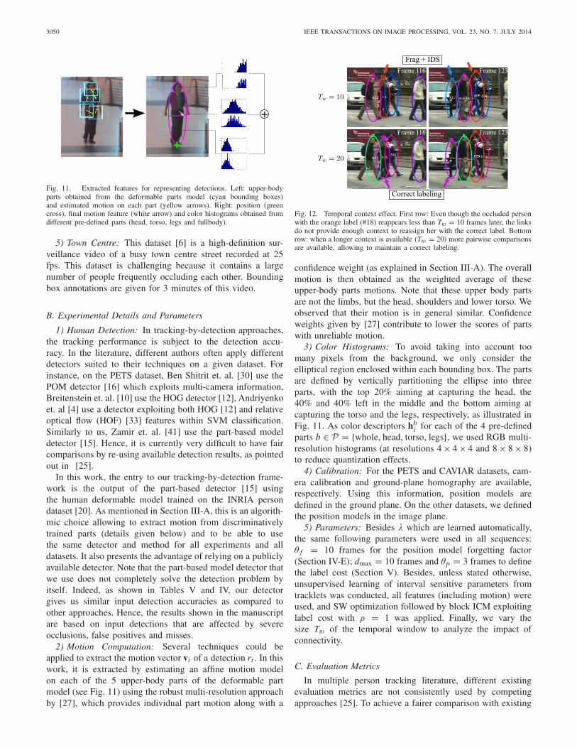
Fig. 11. Extracted features for representing detections. Left: upper-bodyparts obtained from the deformable parts model (cyan bounding boxes)and estimated motion on each part (yellow arrows). Right: position (greencross), final motion feature (white arrow) and color histograms obtained fromdifferent pre-defined parts (head, torso, legs and fullbody).

5) Town Centre: This dataset [6] is a high-definition sur-veillance video of a busy town centre street recorded at 25fps. This dataset is challenging because it contains a largenumber of people frequently occluding each other. Boundingbox annotations are given for 3 minutes of this video.

B. Experimental Details and Parameters

1) Human Detection: In tracking-by-detection approaches,the tracking performance is subject to the detection accu-racy. In the literature, different authors often apply differentdetectors suited to their techniques on a given dataset. Forinstance, on the PETS dataset, Ben Shitrit et. al. [30] use thePOM detector [16] which exploits multi-camera information,Breitenstein et. al. [10] use the HOG detector [12], Andriyenkoet. al [4] use a detector exploiting both HOG [12] and relativeoptical flow (HOF) [33] features within SVM classification.Similarly to us, Zamir et. al. [41] use the part-based modeldetector [15]. Hence, it is currently very difficult to have faircomparisons by re-using available detection results, as pointedout in [25].

In this work, the entry to our tracking-by-detection frame-work is the output of the part-based detector [15] usingthe human deformable model trained on the INRIA persondataset [20]. As mentioned in Section III-A, this is an algorith-mic choice allowing to extract motion from discriminativelytrained parts (details given below) and to be able to usethe same detector and method for all experiments and alldatasets. It also presents the advantage of relying on a publiclyavailable detector. Note that the part-based model detector thatwe use does not completely solve the detection problem byitself. Indeed, as shown in Tables V and IV, our detectorgives us similar input detection accuracies as compared toother approaches. Hence, the results shown in the manuscriptare based on input detections that are affected by severeocclusions, false positives and misses.

2) Motion Computation: Several techniques could beapplied to extract the motion vector vi of a detection ri . In thiswork, it is extracted by estimating an affine motion modelon each of the 5 upper-body parts of the deformable partmodel (see Fig. 11) using the robust multi-resolution approachby [27], which provides individual part motion along with a

Fig. 12. Temporal context effect. First row: Even though the occluded personwith the orange label (#18) reappears less than Tw = 10 frames later, the linksdo not provide enough context to reassign her with the correct label. Bottomrow: when a longer context is available (Tw = 20) more pairwise comparisonsare available, allowing to maintain a correct labeling.

confidence weight (as explained in Section III-A). The overallmotion is then obtained as the weighted average of theseupper-body parts motions. Note that these upper body partsare not the limbs, but the head, shoulders and lower torso. Weobserved that their motion is in general similar. Confidenceweights given by [27] contribute to lower the scores of partswith unreliable motion.

3) Color Histograms: To avoid taking into account toomany pixels from the background, we only consider theelliptical region enclosed within each bounding box. The partsare defined by vertically partitioning the ellipse into threeparts, with the top 20% aiming at capturing the head, the40% and 40% left in the middle and the bottom aiming atcapturing the torso and the legs, respectively, as illustrated inFig. 11. As color descriptors hb

i for each of the 4 pre-definedparts b ∈ P = {whole, head, torso, legs}, we used RGB multi-resolution histograms (at resolutions 4 × 4 × 4 and 8 × 8 × 8)to reduce quantization effects.

4) Calibration: For the PETS and CAVIAR datasets, cam-era calibration and ground-plane homography are available,respectively. Using this information, position models aredefined in the ground plane. On the other datasets, we definedthe position models in the image plane.

5) Parameters: Besides λ which are learned automatically,the same following parameters were used in all sequences:θ f = 10 frames for the position model forgetting factor(Section IV-E); dmax = 10 frames and θp = 3 frames to definethe label cost (Section V). Besides, unless stated otherwise,unsupervised learning of interval sensitive parameters fromtracklets was conducted, all features (including motion) wereused, and SW optimization followed by block ICM exploitinglabel cost with ρ = 1 was applied. Finally, we vary thesize Tw of the temporal window to analyze the impact ofconnectivity.

C. Evaluation Metrics

In multiple person tracking literature, different existingevaluation metrics are not consistently used by competingapproaches [25]. To achieve a fairer comparison with existing


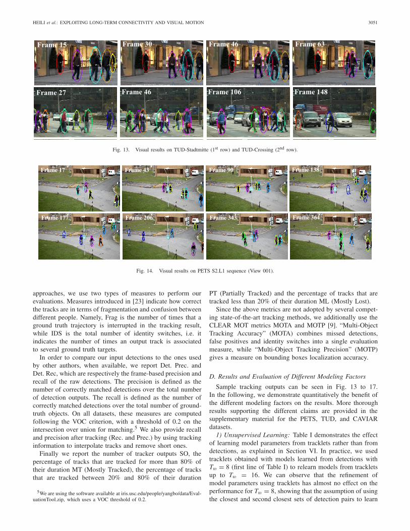
Fig. 13. Visual results on TUD-Stadtmitte (1st row) and TUD-Crossing (2nd row).

Fig. 14. Visual results on PETS S2.L1 sequence (View 001).

approaches, we use two types of measures to perform ourevaluations. Measures introduced in [23] indicate how correctthe tracks are in terms of fragmentation and confusion betweendifferent people. Namely, Frag is the number of times that aground truth trajectory is interrupted in the tracking result,while IDS is the total number of identity switches, i.e. itindicates the number of times an output track is associatedto several ground truth targets.

In order to compare our input detections to the ones usedby other authors, when available, we report Det. Prec. andDet. Rec, which are respectively the frame-based precision andrecall of the raw detections. The precision is defined as thenumber of correctly matched detections over the total numberof detection outputs. The recall is defined as the number ofcorrectly matched detections over the total number of ground-truth objects. On all datasets, these measures are computedfollowing the VOC criterion, with a threshold of 0.2 on theintersection over union for matching.5 We also provide recalland precision after tracking (Rec. and Prec.) by using trackinginformation to interpolate tracks and remove short ones.

Finally we report the number of tracker outputs SO, thepercentage of tracks that are tracked for more than 80% oftheir duration MT (Mostly Tracked), the percentage of tracksthat are tracked between 20% and 80% of their duration

5We are using the software available at iris.usc.edu/people/yangbo/data/Eval-uationTool.zip, which uses a VOC threshold of 0.2.

PT (Partially Tracked) and the percentage of tracks that aretracked less than 20% of their duration ML (Mostly Lost).

Since the above metrics are not adopted by several compet-ing state-of-the-art tracking methods, we additionally use theCLEAR MOT metrics MOTA and MOTP [9]. “Multi-ObjectTracking Accuracy” (MOTA) combines missed detections,false positives and identity switches into a single evaluationmeasure, while “Multi-Object Tracking Precision” (MOTP)gives a measure on bounding boxes localization accuracy.

D. Results and Evaluation of Different Modeling Factors

Sample tracking outputs can be seen in Fig. 13 to 17.In the following, we demonstrate quantitatively the benefit ofthe different modeling factors on the results. More thoroughresults supporting the different claims are provided in thesupplementary material for the PETS, TUD, and CAVIARdatasets.

1) Unsupervised Learning: Table I demonstrates the effectof learning model parameters from tracklets rather than fromdetections, as explained in Section VI. In practice, we usedtracklets obtained with models learned from detections withTw = 8 (first line of Table I) to relearn models from trackletsup to Tw = 16. We can observe that the refinement ofmodel parameters using tracklets has almost no effect on theperformance for Tw = 8, showing that the assumption of usingthe closest and second closest sets of detection pairs to learn


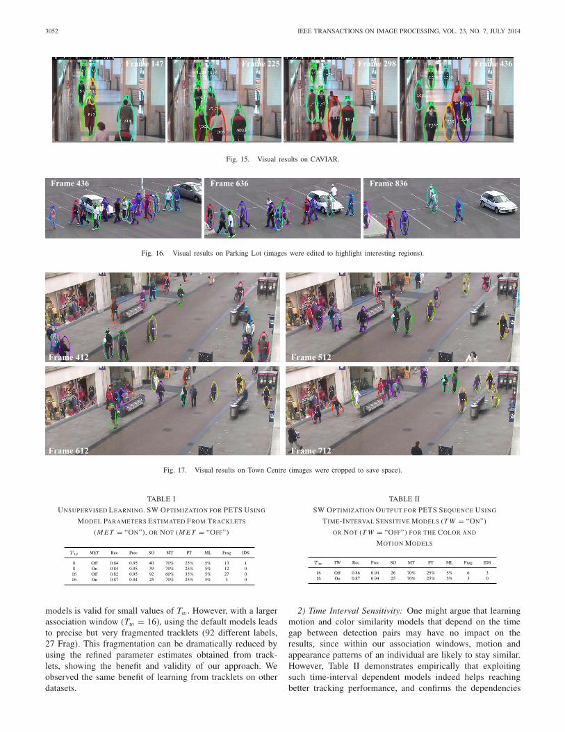
Fig. 15. Visual results on CAVIAR.

Fig. 16. Visual results on Parking Lot (images were edited to highlight interesting regions).

Fig. 17. Visual results on Town Centre (images were cropped to save space).

TABLE I

UNSUPERVISED LEARNING. SW OPTIMIZATION FOR PETS USING

MODEL PARAMETERS ESTIMATED FROM TRACKLETS

(M ET = “ON”), OR NOT (M ET = “OFF”)

models is valid for small values of Tw . However, with a largerassociation window (Tw = 16), using the default models leadsto precise but very fragmented tracklets (92 different labels,27 Frag). This fragmentation can be dramatically reduced byusing the refined parameter estimates obtained from track-lets, showing the benefit and validity of our approach. Weobserved the same benefit of learning from tracklets on otherdatasets.

TABLE II

SW OPTIMIZATION OUTPUT FOR PETS SEQUENCE USING

TIME-INTERVAL SENSITIVE MODELS (T W = “ON”)

OR NOT (T W = “OFF”) FOR THE COLOR AND

MOTION MODELS

2) Time Interval Sensitivity: One might argue that learningmotion and color similarity models that depend on the timegap between detection pairs may have no impact on theresults, since within our association windows, motion andappearance patterns of an individual are likely to stay similar.However, Table II demonstrates empirically that exploitingsuch time-interval dependent models indeed helps reachingbetter tracking performance, and confirms the dependencies


TABLE III

RESULTS ON PETS AND TUD-STADTMITTE SEQUENCES WITH SLIDING

WINDOW OPTIMIZATION. USING THE MOTION FEATURE

(MOTION=“ON”) AND LARGER TEMPORAL WINDOW

Tw PROVIDES BETTER RESULTS

observed on the learned β curves (see Fig. 5 and 9). Whenthe motion and color features between pairs of detections arecollected from tracklets regardless of their time difference(T W = 0), worse results are obtained (the position model islearned normally), resulting in 3 more fragmentations and IDS.A similar behavior has been observed on the other datasets.

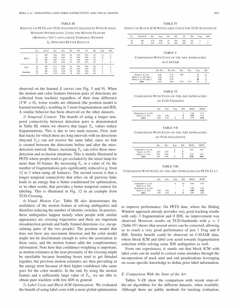
3) Temporal Context: The benefit of using a longer tem-poral connectivity between detection pairs is demonstratedin Table III, where we observe that larger Tw values reducefragmentations. This is due to two main reasons. First, notethat tracks for which there are long intervals with no detections(beyond Tw) can not receive the same label, since no linkis created between the detections before and after the miss-detection interval. Hence, increasing Tw can solve these miss-detection and occlusion situations. This is mainly illustrated inPETS where people tend to get occluded by the street lamp formore than 10 frames. By increasing Tw to a value of 16, thenumber of fragmentations gets significantly reduced (e.g. from12 to 3 when using all features). The second reason is that alonger temporal connectivity that relies on all pairwise linksleads to an energy that is better conditioned for optimization,or in other words, that provides a better temporal context forlabeling. This is illustrated in Fig. 12 in an example fromTUD-Crossing.

4) Visual Motion Cue: Table III also demonstrates theusefulness of the motion feature at solving ambiguities andtherefore reducing the number of identity switches. In practice,these ambiguities happen mainly when people with similarappearance are crossing trajectories and there are importantmissdetection periods and badly framed detections (i.e. encap-sulating parts of the two people). The position model thatdoes not favor any movement direction and the color modelmight not be discriminant enough to solve the association inthese cases, and the motion feature adds the complementaryinformation. Note here that confidence weighting is important,as motion estimates at the near proximity of the crossing mightbe unreliable because bounding boxes tend to get blendedtogether, but previous motion estimates are then prevailing inthe energy term because of their higher confidence (the samegoes for the color models). In the end, by using the motionfeature and a sufficiently large value of Tw, we are able toobtain pure tracklets with few IDS in general.

5) Label Costs and Block ICM Optimization: We evaluatedthe benefit of using label costs with a more global optimization

TABLE IV

EFFECT OF BLOCK ICM WITH LABEL COSTS FOR TUD-STADTMITTE

TABLE V

COMPARISON WITH STATE OF THE ART APPROACHES

ON CAVIAR

TABLE VI

COMPARISON WITH STATE-OF-THE-ART APPROACHES

ON TUD-CROSSING

TABLE VII


ON TUD-STADTMITTE

TABLE VIII

COMPARISON WITH STATE-OF-THE-ART APPROACHES ON PETS S2.L1

to improve performance. On PETS data, where the SlidingWindow approach already provides very good tracking resultswith only 3 fragmentation and 0 IDS, no improvement wasobserved. However, results on TUD-Stadtmitte with ρ = 3(Table IV) shows that several errors can be corrected, allowingus to reach a very good performance of just 1 Frag and 0IDS. Similar benefit could be observed on CAVIAR data,where block ICM and label cost acted towards fragmentationreduction while solving some IDS ambiguities as well.

From our experiences, it stands out that block ICM withlabel costs can be useful to correct some mistakes through theincorporation of track start and end penalizations leveragingon scene-specific knowledge to define prior label information.

E. Comparison With the State of the Art

Tables V–IX show the comparison with recent state-of-the-art algorithms for the different datasets, when available.Although there are public methods for tracking evaluation,


there is a lack of a unique standard procedure (i.e, someauthors use MOT metrics while others use fragmentation andIDS). This makes fair comparison against several methods,including recent ones, difficult, as pointed by Milan et. al. [25].In this paper, we evaluate our performance with differentexisting metrics to allow comparison with existing approachesthat have some similarities to our proposal. Note as wellthat, as discussed in Section VIII-B, different authors oftenuse different detectors. For the sake of having more detailedcomparisons, we also report and discuss the input detectionrecall and precision of our detections and compare them tothose of the detections provided by the different authors, whenavailable.

On the CAVIAR dataset, Table V compares our resultsobtained with an association horizon of 1.5 second (Tw =38) and default parameters, with the approaches from [19]and [42]. Note first that our detector delivers lower per-formance, with a worse detection recall for a comparabledetection precision. Nevertheless, the table shows that weoutperform [19] in terms of Frag and IDS. As comparedto the network flow formulation of [42] (algo. 1), we reachan almost identical number of IDS (8 vs. 7) but with muchless fragmented tracks (38 vs. 58). When adding an explicitocclusion model on top of the flow model (algo. 2), the methodin [42] reduces the number of fragmentations to 20, but thisis at the cost of a higher number of IDS (15). Our approachthus offers a good tradeoff between their methods.

For the TUD and PETS datasets, we report our resultsobtained with Tw = 20 and Tw = 16, respectively. In theTUD-Crossing sequence which contains heavy occlusions, weobtain 1 Frag and 0 IDS, outperforming the method of [10](2 IDS) and we equal [41] in terms of IDS. However, theyboth present a better MOTA score. This can be explainedby the fact that MOTA takes into account not only IDS, butalso tracking precision and recall. In this sequence, people areoften occluded because they walk next to each other, and thistranslates into low detection recall. For instance, by the endof the sequence we miss a subject due to such an occlusion,because we did not get any detection in the first place. Sincethe proposed method does not attempt to propagate detectionsnor extrapolate tracklets, such missdetections penalize thetracking recall, and ultimately the MOTA. The methods of [10]and [41] generate candidate detections by using particles andvirtual nodes, respectively, potentially overcoming problemswith missing detections due to occlusion. Despite the lack ofdetections, in this sequence our method obtains pure tracklets,with only 1 fragmentation.

On TUD-Stadtmitte, we outperform [4] both in terms ofFrag, IDS and MOT metrics. We reach similar results as [41]and [37], with 1 Frag and 0 IDS. However, we outperform [41]in terms of MOT metrics.

On PETS, we clearly outperform other techniques insofaras we reach 0 IDS. The authors of [41] obtain comparableMOT metrics but with a much higher number of 8 IDS. Itcan be noted that one of our fragmentations is due to the factthat a person going out of the scene and coming back lateris annotated as one single ground truth object. This situationis out of the scope of this paper, as we do not tackle the

TABLE IX


ON PARKING LOT AND TOWN CENTRE

re-identification problem. Another fragmentation is due to avery long occlusion by the street lamp (more than 10 seconds).

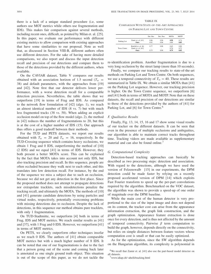
Finally, we compare our tracking results to state-of-the-artmethods on Parking Lot and Town Centre. On both sequences,we use a temporal connectivity of Tw = 40. These results aresummarized in Table IX. We obtain a similar MOTA than [41]on the Parking Lot sequence. However, our tracking precisionis higher. On the Town Centre sequence, we outperform [6]and [41] both in terms of MOTA and MOTP. Note that on thesedatasets, the recall and precision of our detections are similarto those of the detections provided by the authors of [41] forParking Lot, and [6] for Town Centre.6

F. Qualitative Results

Finally, Fig. 13, 14, 15, 16 and 17 show some visual resultsof our tracker on the different datasets. It can be seen thateven in the presence of multiple occlusions and ambiguities,our algorithm is able to maintain correct tracks throughouttime. Tracking videos are made available as supplementarymaterial and can also be found online.7

G. Computational Complexity

Detection-based tracking approaches can basically bedescribed as two processing steps: detection and association.With regard to the detections, although we have used theversion of Felzenswalb [15] in our experiments, the DPMdetection could be made faster by relying on a recentlyproposed accelerated version of DPM [14] which exploitsFast Fourier transform to speed up the per-part convolutionsrequired by the algorithm. Benchmarked on the VOC dataset,the algorithm was shown to provide a speed-up of one orderof magnitude over the DPM baseline.

While the main cost of the human detector is very pro-portional to the size of the input image and does not dependon its content, the tracker cost can arise from the appearanceinformation extraction, the graph link construction, and thegraph optimization. Appearance feature extraction is doneonce for every detection, and is thus not affected by the amountof temporal connectivity. Pairwise β term computation tobuild the graph, however, depends directly on the connectivity,but relies on simple distances between feature vectors whosecomputation cost is small or that can be easily optimized.

As for the optimization, since the SW algorithm dependson the Hungarian algorithm, its complexity is polynomial in

6We recall that Zamir et. al. [41] also use the part-based model detector onall datasets.

7www.idiap.ch/~aheili/tracking.html


O(n3), where n is the maximum between the number of detec-tions in the current frame and the number of current tracks inthe sliding window. Therefore, longer term connectivity doesnot necessarily imply an increase in complexity. Indeed, asthere are typically fewer fragmentations (and thus less tracks)when using longer temporal windows, the complexity mighteven be reduced. Similarly, block ICM is optimized usingthe Hungarian algorithm, and its complexity is polynomial inthe maximum of the number of tracks before and after thecurrently optimized frame in the ICM sweep.

To give an idea about the computational complexity of ourtracking algorithm, we report the following average processingtimes per frame on the medium crowded scene of PETS2009 with an association horizon Tw of 2 seconds, testedon a 2.9 GHz Intel Core i7 laptop with 8GB of RAM andassuming detections are available: 150ms for visual motionestimation and color features extraction; 180ms for computingthe pairwise β terms; 60ms and 280ms for SW and Block ICMoptimization, respectively. Note that we have an unoptimizedimplementation in Python with no threading. Online trackingprocessing could be achieved by optimizing algorithmic steps8

or selecting the time steps at which applying Block ICMcould be useful, or through code optimization (programminglanguage, multi-threading, etc.) as well as by processing videosat a lower framerate.

IX. CONCLUSION

We presented a CRF model for detection-based multi-persontracking. Contrarily to other methods, it exploits longer-termconnectivities between pairs of detections. Moreover, it relieson pairwise similarity and dissimilarity factors defined atthe detection level, based on position, color and also visualmotion cues, along with a feature-specific factor weightingscheme that accounts for feature reliability. The model alsoincorporates a label field prior penalizing unrealistic solutions,leveraging on track and scene characteristics like duration andstart/end zones. Experiments on public datasets and compar-isons with state-of-the-art approaches validated the differentmodeling steps, such as the use of a long time horizon Tw

with a higher density of connections that better constrains themodels and provides more pairwise comparisons to assess thelabeling, or an unsupervised learning scheme of time-intervalsensitive model parameters.

There are several possibilities to extend our work. First,rather than using the same model parameters for the wholetest sequence, unsupervised learning or adaptation of modelparameters could be done online by considering detectionoutputs until the given instant while performing trackingon long videos. Second, in addition to the exploitation ofreliability factors to handle corrupted features due to detectionoverlap, perspective reasoning as well as finer pixel-levelsegmentation (e.g. relying on motion [26]) could be used toselect only the relevant pixels for computing the appearanceand motion descriptors associated with a detection. Third,

8For instance using simple and quick procedures to trim unnecessary links inthe graph, e.g. by not creating links between detection pairs that are separatedby unrealistic distances.

in order to handle the high-level of miss-detections that cannegatively impact our algorithm, short term forward and/orbackward propagations of detections could be generated anddirectly used as another pairwise association cue in our frame-work. Furthermore, to handle long occlusions (beyond 3s andmore), higher order appearance re-identification factor termspotentially relying on online learned discriminative modelslike [5] should be defined and exploited at another hierarchicallevel. Finally, to better handle crowd and small group movinginteractions, high-order dynamical prior model taking intoaccount multiple tracks jointly could be defined like in [7] andused to constrain the solution space in the global optimizationstage.

REFERENCES

[1] (2012, Oct.). PETS 2009 Benchmark Data [Online]. Available:http://www.cvg.rdg.ac.uk/PETS2009/a.html

[2] (2011, Jun.). CAVIAR Test Case Scenarios [Online]. Available:http://groups.inf.ed.ac.uk/vision/CAVIAR/CAVIARDATA1/

[3] A. Andriyenko and K. Schindler, “Multi-target tracking by contin-uous energy minimization,” in Proc. IEEE Conf. CVPR, Jun. 2011,pp. 1265–1272.

[4] A. Andriyenko, K. Schindler, and S. Roth, “Discrete-continuous opti-mization for multi-target tracking,” in Proc. IEEE Conf. CVPR,Jun. 2012, pp. 1926–1933.

[5] S. Bak, D. P. Chau, J. Badie, E. Corvee, F. Bremond, and M. Thonnat,“Multi-target tracking by discriminative analysis on Riemannian mani-fold,” in Proc. IEEE ICIP, Sep./Oct. 2012, pp. 1605–1608.

[6] B. Benfold and I. Reid, “Stable multi-target tracking in real-time sur-veillance video,” in Proc. IEEE Conf. CVPR, Jun. 2011, pp. 3457–3464.

[7] J. Berclaz, F. Fleuret, and P. Fua, “Multi-camera tracking and atyp-ical motion detection with behavioral maps,” in Proc. ECCV, 2008,pp. 112–125.

[8] J. Berclaz, F. Fleuret, and P. Fua, “Multiple object tracking using flowlinear programming,” in Proc. 12th IEEE Int. Workshop Winter-PETS,Dec. 2009, pp. 1–8.

[9] K. Bernardin and R. Stiefelhagen, “Evaluating multiple object trackingperformance: The CLEAR MOT metrics,” J. Image Video Process.,vol. 2008, pp. 1:1–1:10, Feb. 2008.

[10] M. D. Breitenstein, F. Reichlin, B. Leibe, E. Koller-Meier, andL. Van Gool, “Online multiperson tracking-by-detection from a single,uncalibrated camera,” IEEE Trans. Pattern Anal. Mach. Intell., vol. 33,no. 9, pp. 1820–1833, Sep. 2011.

[11] R. T. Collins, “Multitarget data association with higher-order motionmodels,” in Proc. IEEE Conf. CVPR, Jun. 2012, pp. 1744–1751.

[12] N. Dalal and B. Triggs, “Histograms of oriented gradients for humandetection,” in Proc. IEEE Int. CVPR, Jun. 2005, pp. 886–893.

[13] P. Dollar, S. Belongie, and P. Perona, “The fastest pedestrian detectorin the west,” in Proc. BMVC, 2010, pp. 68.1–68.11.

[14] C. Dubout and F. Fleuret, “Exact acceleration of linear object detectors,”in Proc. ECCV, 2012, pp. 301–311.

[15] P. F. Felzenszwalb, R. B. Girshick, D. McAllester, and D. Ramanan,“Object detection with discriminatively trained part-based models,”IEEE Trans. Pattern Anal. Mach. Intell., vol. 32, no. 9, pp. 1627–1645,Sep. 2010.

[16] F. Fleuret, J. Berclaz, R. Lengagne, and P. Fua, “Multicamera peopletracking with a probabilistic occupancy map,” IEEE Trans. Pattern Anal.Mach. Intell., vol. 30, no. 2, pp. 267–282, Feb. 2008.

[17] A. Heili, C. Chen, and J.-M. Odobez, “Detection-based multi-humantracking using a CRF model,” in Proc. IEEE ICCV Workshop, Nov.2011, pp. 1673–1680.

[18] A. Heili and J.-M. Odobez, “Parameter estimation and contextualadaptation for a multi-object tracking CRF model,” in Proc. IEEE Int.Workshop PETS, Jan. 2013, pp. 14–21.

[19] C. Huang, B. Wu, and R. Nevatia, “Robust object tracking by hierar-chical association of detection responses,” in Proc. 10th ECCV, 2008,pp. 788–801.

[20] (2011, Jun.). INRIA Person Dataset [Online]. Available:http://pascal.inrialpes.fr/data/human/

[21] V. Kolmogorov and R. Zabin, “What energy functions can be minimizedvia graph cuts?” IEEE Trans. Pattern Anal. Mach. Intell., vol. 26, no. 2,pp. 147–159, Feb. 2004.


[22] C.-H. Kuo and R. Nevatia, “How does person identity recognitionhelp multi-person tracking?” in Proc. IEEE Conf. CVPR, Jun. 2011,pp. 1217–1224.

[23] Y. Li, C. Huang, and R. Nevatia, “Learning to associate: HybridBoostedmulti-target tracker for crowded scene,” in Proc. IEEE Conf. CVPR,Jun. 2009, pp. 2953–2960.

[24] E. Maggio and A. Cavallaro, “Learning scene context for multiple objecttracking,” IEEE Trans. Image Process., vol. 18, no. 8, pp. 1873–1884,Aug. 2009.

[25] A. Milan, K. Schindler, and S. Roth, “Challenges of ground truthevaluation of multi-target tracking,” in Proc. IEEE Conf. CVPRW,Jun. 2013, pp. 735–742.

[26] J.-M. Odobez and P. Bouthemy, “MRF-based motion segmentationexploiting a 2D motion model robust estimation,” in Proc. IEEE Int.Conf. Image Process., Oct. 1995, pp. 628–631.

[27] J.-M. Odobez and P. Bouthemy, “Robust multiresolution estimation ofparametric motion models,” J. Vis. Commun. Image Represent., vol. 6,no. 4, pp. 348–365, 1995.

[28] H. Pirsiavash, D. Ramanan, and C. C. Fowlkes, “Globally-optimalgreedy algorithms for tracking a variable number of objects,” in Proc.IEEE Conf. CVPR, Jun. 2011, pp. 1201–1208.

[29] M. Rodriguez, I. Laptev, J. Sivic, and J.-Y. Audibert, “Density-aware per-son detection and tracking in crowds,” in Proc. IEEE ICCV, Nov. 2011,pp. 2423–2430.

[30] H. Ben Shitrit, J. Berclaz, F. Fleuret, and P. Fua, “Tracking multiplepeople under global appearance constraints,” in Proc. IEEE ICCV,Nov. 2011, pp. 137–144.

[31] B. Song, T.-Y. Jeng, E. Staudt, and A. K. R. Chowdhury, “A stochasticgraph evolution framework for robust multi-target tracking,” in Proc.ECCV, 2010, pp. 605–619.

[32] X. Song, X. Shao, H. Zhao, J. Cui, R. Shibasaki, and H. Zha, “Anonline approach: Learning-semantic-scene-by-tracking and tracking-by-learning-semantic-scene,” in Proc. IEEE Conf. CVPR, Jun. 2010,pp. 739–746.

[33] S. Walk, N. Majer, K. Schindler, and B. Schiele, “New featuresand insights for pedestrian detection,” in Proc. IEEE Conf. CVPR,San Francisco, CA, USA, Jun. 2010, pp. 1030–1037.

[34] Z. Wu, T. H. Kunz, and M. Betke, “Efficient track linking methodsfor track graphs using network-flow and set-cover techniques,” in Proc.IEEE Conf. CVPR, Jun. 2011, pp. 1185–1192.

[35] B. Yang, C. Huang, and R. Nevatia, “Learning affinities and dependen-cies for multi-target tracking using a CRF model,” in Proc. IEEE Conf.CVPR, Jun. 2011, pp. 1233–1240.

[36] B. Yang and R. Nevatia, “Multi-target tracking by online learning ofnon-linear motion patterns and robust appearance models,” in Proc. IEEEConf. CVPR, Jun. 2012, pp. 1918–1925.

[37] B. Yang and R. Nevatia, “An online learned CRF model for multi-targettracking,” in Proc. IEEE Conf. CVPR, Jun. 2012, pp. 2034–2041.

[38] M. Yang, Y. Wu, and G. Hua, “Context-aware visual tracking,” IEEETrans. Pattern Anal. Mach. Intell., vol. 31, no. 7, pp. 1195–1209,Jul. 2009.

[39] J. Yao and J.-M. Odobez, “Multi-camera multi-person 3D space track-ing with MCMC in surveillance scenarios,” in Proc. ECCV-M2SFA2,Marseille, France, Oct. 2008.

[40] A. Yilmaz, O. Javed, and M. Shah, “Object tracking: A survey,” ACMComput. Surv., vol. 38, no. 4, p. 13, 2006.

[41] A. R. Zamir, A. Dehghan, and M. Shah, “GMCP-tracker: Global multi-object tracking using generalized minimum clique graphs,” in Proc.ECCV, 2012, pp. 343–356.

[42] L. Zhang, Y. Li, and R. Nevatia, “Global data association for multi-objecttracking using network flows,” in Proc. IEEE Conf. CVPR, Jun. 2008,pp. 1–8.

Alexandre Heili (S’11) recived the degreefrom Télécom Physique Strasbourg, Illkirch-Graffenstaden, France, and the M.Sc. degreein computer vision and medical robotics fromUniversité de Strasbourg, Strasbourg, France,in 2009. He is currently pursuing the Ph.D.degree with the Idiap Research Institute, Martigny,Switzerland, and École Polytechnique Fédérale deLausanne, Lausanne, Switzerland.

Adolfo López-Méndez received the B.Sc. degreeand master’s degree in signal theory and communi-cations from the Technical University of Catalonia,Barcelona, Spain, in 2007 and 2009, respectively,where he received the Ph.D. degree. During thisperiod, he was involved in several national and Euro-pean projects (VISION, PROVEC, CHIL, ACTIBIO,and FASCINATE). In 2012, he became a Post-Doctoral Researcher at the Idiap Research Institute,Martigny, Switzerland. His research interests includetracking, action, and gesture recognition, markerless

motion capture, and machine learning.

Jean-Marc Odobez (M’03) received the degreefrom École Nationale Supérieure de Télécommuni-cations de Bretagne, Plouzané, France, in 1990, andthe Ph.D. degree from INRIA, Rennes University,Rennes, France, in 1994. He was an AssociateProfessor of Computer Science with the Univer-sité du Maine, Le Mans, France, from 1996 to2001. He is currently a Senior Researcher with theIdiap Research Institute, Martigny, Switzerland, andÉcole Polytechnique Fédérale de Lausanne, Lau-sanne, Switzerland, where he is the Director of the

Perception and Activity Understanding Team. His main areas of researchare computer vision and machine learning techniques applied to multimediacontent analysis, tracking, and human activity and behavior recognition. Hehas authored and co-authored more than 100 papers in international journalsand conferences. He has been the principal investigator of 10 European andSwiss projects. He holds two patents on video motion analysis. He is the Co-Founder of the Swiss Klewel SA Company, Martigny, where he is involved inthe intelligent capture, indexing, and Web casting of multimedia conferences.He is an Associate Editor of the Machine Vision and Application journal.