


Bahasa
Halaman
Hukum

Evaluating eutrophication management scenarios in
the Baltic Sea using species distribution modelling
Ulf Bergstr€om1*, G€oran Sundblad2, Anna-Leena Downie3, Martin Snickars4,
Christoffer Bostr€om4 and Mats Lindegarth5
1Swedish University of Agricultural Sciences, Department of Aquatic Resources, Institute of Coastal Research,
Skolgatan 6, 74242 €Oregrund, Sweden; 2AquaBiota Water Research, L€ojtnantsgatan 25, 11550 Stockholm, Sweden;3Finnish Environment Institute, Marine Research Centre, PO Box 140, 00251 Helsinki, Finland; 4Department of
Biosciences, Environmental and Marine Biology, �Abo Akademi University, Artillerigatan 6, 20520 �Abo, Finland; and5Department of Biological and Environmental Sciences, University of Gothenburg, Tj€arn€o, 45296 Str€omstad, Sweden
Summary
1. Eutrophication is severely affecting species distributions and ecosystem functioning in
coastal areas. Targets for eutrophication reduction have been set in the Baltic Sea Action
Plan (BSAP) using Secchi depth, a measure of water transparency, as the main status indica-
tor. Despite the high economic costs involved, the potential effects of this political decision
on key species and habitats have not been assessed.
2. In a case study including species central to coastal ecosystem functioning, we modelled the
effects of changing Secchi depth on the distribution of bladderwrack Fucus vesiculosus and
eelgrass Zostera marina vegetation as well as recruitment areas of the main predatory fish spe-
cies, perch Perca fluviatilis and pikeperch Sander lucioperca. Specifically, we explored the
effects of changing Secchi depth on species distributions under a set of scenarios based on the
BSAP, using three fundamentally different modelling techniques: maximum entropy, general-
ized additive and random forest modelling.
3. Improved Secchi depth (reduced eutrophication) was predicted to cause a substantial
increase in the distribution of bladderwrack, while the distribution of eelgrass remained lar-
gely unaffected. For the fish, a large increase in perch recruitment areas was predicted and a
concurrent decrease in recruitment areas of pikeperch. These changes are likely to have effects
on biodiversity and ecosystem services.
4. The three modelling methods exposed differences in the quantitative predictions for species
with a weaker coupling to Secchi depth. Qualitatively, however, the results were consistent
for all species.
5. Synthesis and applications. We show how ecological effects of environmental policies can
be evaluated in an explicit spatial context using species distribution modelling. The model-
specific responses to changes in eutrophication status emphasize the importance of using
ensemble modelling for exploring how species distributions may respond to alternative
management regimes. A pronounced difference in response between species suggests that
eutrophication mitigation will have consequences for ecosystem functioning, and thus eco-
system goods and services, by inducing changes in the simple food webs of the Baltic Sea.
These model predictions form a basis for spatially explicit cost-benefit estimates under dif-
ferent scenarios, providing valuable information for both decision-makers and the wider
society.
Key-words: Baltic Sea Action Plan, ensemble modelling, GAM, Maxent, Random Forest,
scenario analysis, Secchi depth, species distribution models
*Correspondence author. E-mail: [email protected].
© 2013 The Authors. Journal of Applied Ecology © 2013 British Ecological Society
Journal of Applied Ecology 2013 doi: 10.1111/1365-2664.12083
Introduction
As a result of growing human populations and an associ-
ated increase in competition for space, loss of habitat is
now one of the major threats to biodiversity and the ser-
vices provided by ecosystems (Sih, Jonsson & Luikart
2000). Pressures on habitats are particularly severe in
coastal areas, as a consequence of the high concentration
of human activities (Airoldi & Beck 2007). In order to
better manage conflicts of interest, minimize negative
impacts and promote sustainable use of coastal environ-
ments, tools and information systems for marine spatial
planning are currently the focus of extensive efforts. One
area of particular interest for efficient planning is the
development of methods for coupling human pressures
and ecological effects, that is, for predicting the ecological
consequences of alternative policy and management
scenarios.
The complexity of ecosystems, however, makes predic-
tion of ecological responses to environmental change
extremely challenging, and scenario-based assessments are
still in their infancy (Coreau et al. 2009; Elith & Leath-
wick 2009). Scenarios are sets of expectations about plau-
sible futures, which aim to explore the range of potential
outcomes starting from a known situation, to aid in man-
agement planning (Bennett et al. 2003). Scenario analysis
is often perceived only as a qualitative description of pos-
sible futures, given a set of assumptions of driving forces
or extrinsic stressors. However, using scenarios in combi-
nation with predictive ecological models may be a way of
producing quantitative estimates of the span of potential
future outcomes, encompassing different sources of uncer-
tainty (Coreau et al. 2009).
For ecology to grow into a fully integrated part of deci-
sion-making in society, taking these difficult steps towards
a quantitative and predictive discipline is crucial (Pereira
et al. 2010). One branch that has emerged within predic-
tive ecology is species distribution modelling, in which
species–environment relationships are described statisti-
cally and used to make spatial predictions of species dis-
tributions across space and time (Elith & Leathwick
2009). Species distribution models (SDMs) have the
potential to be used as tools for exploring management
scenarios relating to the conservation of species and habi-
tats (Robinson et al. 2011). So far, SDMs have primarily
been used in large-scale studies of climate change effects
(e.g. Keith et al. 2008; Ara�ujo et al. 2011), while their
potential for exploring management options relating to
human pressures that can be managed at a regional scale
is largely unknown. The basis of the method is that by
including a measure of the human pressure(s) of interest
as predictor variable(s) in the model, the effects of
changes in the pressure may be explored. Adding the
spatial component of the SDM into a scenario modelling
approach greatly enhances the information that can be
gained from relating a change in a pressure to changes in
the species of interest, when compared to a purely correlative
approach. The ability to define spatially explicit changes
allows for a more locally relevant and quantitative assess-
ment of expected change, providing answers to the ques-
tions of how much change and where. For this approach
to be successful, the pressure variable should have a
direct, mechanistic effect on the modelled response vari-
able. Further, the future level and distribution of the pres-
sure variable expected under the scenario being evaluated
is needed in order to make spatial predictions of the
modelled species.
In the current study, we set out to test the utility of
SDMs for studying scenarios relating to eutrophication
mitigation measures in the Baltic Sea. Eutrophication, due
to excessive phosphorus and nitrogen loads, is one of the
most serious threats to coastal ecosystems worldwide
(Cloern 2001), including the semi-enclosed Baltic Sea
(Korpinen et al. 2012). The high nutrient concentrations
give rise to excessive growth of planktonic and filamen-
tous algae, which leads to shading, smothering and
reduced recruitment success of perennial macrophytes in
the shallow sublittoral (Berger et al. 2004; Krause-Jensen
et al. 2008), as well as oxygen deficiency and habitat deg-
radation with severe negative effects on ecosystem func-
tioning and the goods and services provided by the sea
(R€onnberg & Bonsdorff 2004; Diaz & Rosenberg 2008).
These problems, in combination with the requirements of
the EU Marine Strategy Framework Directive and the
Water Framework Directive, have led the member states
of Helsinki Commission (HELCOM, the executive body
of the Convention on the Protection of the Marine Envi-
ronment of the Baltic Sea Area) to take action against
eutrophication in the Baltic Sea Action Plan (BSAP). This
action plan was adopted in 2007 by all countries sur-
rounding the Baltic Sea (HELCOM 2007a). It has set up
a number of environmental objectives for 2021, relating
to eutrophication, hazardous substances, maritime activi-
ties and biodiversity conservation (Backer et al. 2010).
The main indicator for eutrophication is water transpar-
ency measured as mean summer Secchi disc depth
(HELCOM 2007a). The Secchi disc method (Preisendorfer
1986) is a simple measure of the amount of phytoplank-
ton in the water column, and long time-series are avail-
able. While phytoplankton only accounts for 17–40% of
light attenuation in the study area, there is a strong rela-
tionship between light attenuation and the chlorophyll a
concentration in the water column, indicating that Secchi
depth is a good indicator of eutrophication status
(Fleming-Lehtinen & Laamanen 2012). Specific target and
reference levels for water transparency have been set for
the different basins of the Baltic Sea. The reference levels
are based on historical data, while the target levels are set
to 25% lower transparency than the reference level.
For the Baltic Sea region, the countrywise nutrient
reductions required to reach these goals, as well as the
necessary measures, have been defined (HELCOM 2007b;
Wulff et al. 2007). Costs associated with eutrophication
mitigation are high, and therefore, it is important not
© 2013 The Authors. Journal of Applied Ecology © 2013 British Ecological Society, Journal of Applied Ecology
2 U. Bergstr€om et al.

only to consider the cost-efficiency of different actions
(Elofsson 2010), but also to study more in detail how eco-
system components and functions may respond to a
decrease in eutrophication. So far, however, the potential
effects of the agreed reduction in nutrient loads on the
ecosystems and associated goods and services have only
been afforded a cursory evaluation. Qualitative studies
indicate that most provisioning, regulating and cultural
services of coastal habitats would increase with an
improved eutrophication situation (R€onnb€ack et al. 2007;
BalticSTERN 2013; Ahtiainen & Vanhatalo 2012). How-
ever, detailed studies, entailing quantitative measures of
how species distributions and ecosystem services may
change with a decrease in eutrophication, are lacking.
In this paper, we show how SDMs can be used for
exploring the effects of alternative management measures
on the distribution of habitats. We utilize a simple sce-
nario approach, where we account for different sources of
uncertainty. Specifically, we use an ensemble of species
distribution models for studying the consequences of
eutrophication mitigation on the distribution of key
coastal macrophyte and fish species in a 40 000-km2
archipelago area in the northern Baltic Sea. The angio-
sperm eelgrass Zostera marina L. and the brown alga
bladderwrack Fucus vesiculosus L. are both considered to
be sensitive to eutrophication and changes in water trans-
parency (e.g. Berger et al. 2004; Krause-Jensen et al.
2008), and as such, they are used as important indicators
for monitoring environmental status in most Baltic coun-
tries (B€ack et al. 2006; Schories, Pehlke & Selig 2009).
The fish species perch Perca fluviatilis L. and pikeperch
Sander lucioperca L., differ in their preferences for recruit-
ment areas with respect to water transparency, with perch
preferring clear water and pikeperch turbid waters
(Sandstr€om & Kar�as 2002; Ljunggren & Sandstr€om 2007;
Veneranta et al. 2011). Based on this knowledge of eutro-
phication responses of the study species, we hypothesized
that the distribution of eelgrass and bladderwrack and
recruitment areas of perch would increase with a higher
water transparency, while recruitment areas of pikeperch
would decrease.
Materials and methods
STUDY AREA AND SPECIES
The study area is located in the northern Baltic Sea, covering
the extensive archipelago between Sweden and Finland (Fig. 1).
The 40 000-km2 area is characterized by high topographic com-
plexity, this being the world’s largest archipelago by the number
of islands. The convoluted shoreline and mosaic of islands create
strong small-scale environmental gradients and patchy habitat
distributions. The salinity range is 4–7 psu, and the area encom-
passes a wide range of wave exposure conditions, from enclosed
bays in the innermost parts of the archipelagos to open sea.
The Baltic Sea is a young brackish-water sea (approximately
4000 years in its current state) characterized by low diversity
and a mix of marine and freshwater organisms, with a few dom-
inant species found in high abundances (Bonsdorff & Blomqvist
1993).
The main canopy-forming alga on hard substrates in the north-
ern Baltic Sea is bladderwrack, while soft substrates are inhabited
by numerous species of angiosperms of freshwater origin and a
few marine ones, most importantly eelgrass. Bladderwrack and
eelgrass are both key habitat-forming species in the area; by pro-
viding complex structures to their respective habitats, they consti-
tute the basis for diverse and highly productive coastal biotopes
(Bostr€om et al. 2006; Wikstr€om & Kautsky 2007). The demersal
fish community of the area is dominated by freshwater percids
and cyprinids together with whitefish and marine flatfishes. Two
of the dominating fish species are the large predators perch and
pikeperch, which are also among the most important species for
both recreational and commercial fisheries (Lehtonen, Hansson &
Winkler 1996; �Adjers et al. 2006). Both species have specific
habitat requirements for their recruitment, selecting shallow, shel-
tered bays that warm up early in spring (Lehtonen, Hansson &
Winkler 1996; Snickars et al. 2010). One important aspect of the
ecology of these two species is that they are both sensitive to the
Fig. 1. Map of the study area in the
northern Baltic Sea. Sampling stations for
bladderwrack, eelgrass, perch and pike-
perch are shown on a background of cur-
rent mean summer Secchi depth.
© 2013 The Authors. Journal of Applied Ecology © 2013 British Ecological Society, Journal of Applied Ecology
Evaluating eutrophication management scenarios 3
level of water transparency, perch preferring clear waters and
pikeperch turbid waters (see Introduction).
DATA SETS
Field data on the occurrence, that is, presence and absence records,
of the study species (Fig. 1) were collated from a number of sources
(see Appendix S1, Supporting information). Bladderwrack (1139
records, including 333 presences) and eelgrass (1340 records,
including 151 presences) were compiled from drop-video, ROV,
snorkelling and scuba-dive surveys performed in 2004–2009. The
data sets on fish recruitment areas came from studies performed
in 2003–2009, using visual transect survey by snorkelling for
perch egg strands (4039 records, including 302 presences) and
small underwater detonations for young-of-the-year pikeperch
(570 records, including 33 presences).
Three environmental variables with effects on species distribu-
tions were used as predictors in the modelling – water depth,
wave exposure and Secchi depth (Eriksson & Bergstr€om 2005;
Sundblad, Bergstr€om & Sandstr€om 2011). All environmental vari-
able rasters had a grid cell size of 25 m. The water depth raster
was interpolated using depth data available from official sea
charts. The wave exposure raster, log-transformed to normalize
distributions, was calculated with the Wave Impact software
(Isæus 2004), which combines fetch calculations with wind condi-
tions and also accounts for refraction and diffraction effects. A
raster of Secchi depth, the pressure variable in the scenarios, was
produced using a generalized additive model (GAM) based on
monitoring and inventory data from 2000–2008 (see Appendix
S2, Supporting information). The resulting raster showed mean
summer (months 5–9) water transparency, as this time period is
used as an indicator for eutrophication in the BSAP. The model
explained 85% of the variation and evaluation against withheld
data resulted in an r2 of 0�79 and a root mean square error of
0�69 m. Secchi depth rasters for each scenario were produced by
recalculating the current Secchi depth values, multiplying each
grid cell in the raster according to the percentage change expected
under the scenarios described below.
SCENARIOS
The effects of changes in water transparency on the predicted
spatial distribution of the study species were explored by adjust-
ing the Secchi depth according to a set of scenarios. We specified
three scenarios relating to changes in water transparency, based
on the BSAP target and reference levels as well as the current
trend of Secchi depth in the study area and surrounding waters.
Secchi depth monitoring data show that in offshore areas of the
Baltic Proper and the Bothnian Sea, water transparency contin-
ues to decrease (HELCOM 2009). Long-term data from the study
area collated in this study and in HELCOM (2012) show
decreases or no trends, while in areas close to local eutrophica-
tion sources such as Stockholm even increases in Secchi depth
have been observed (Karlsson et al. 2010).
The scenarios were defined based on the difference between the
current level of water transparency and the BSAP target and refer-
ence levels (HELCOM 2007a), according to the following: (1)
Return to BSAP reference level: according to the BSAP, the refer-
ence level for water transparency is 9�3 m and the current level is
6�3 m in the Baltic Proper. A return to the reference level corre-
sponds to a 48% increase in Secchi depth. (2) Return to BSAP
target level: for the Baltic Proper, a return to the BSAP target is
defined as a 25% deviation from the reference level. This corre-
sponds to an 11% increase in water transparency compared to the
current situation. (3) Business-as-usual: although not fully consis-
tent, the general trend in available data suggests that the Secchi
depth is still decreasing at a rate that corresponds to approximately
a 10% decrease until 2021, for which the BSAP targets are set. The
business-as-usual scenario is therefore set to �10%.
The three scenarios of this study only involve changes in Secchi
depth, all other variables being constant. Thus, potential changes
in other pressure variables relating to, for example, climate
change and physical habitat loss are not considered in the study.
To be able to make predictions for the different scenarios, the
Secchi depth map was changed according to the levels specified
above. To account for the uncertain effects of the ongoing eutro-
phication mitigation actions and to increase interpretability of the
results, predictions for three more levels of change in Secchi
depth were calculated: increases by 20, 30 and 40%. Making pre-
dictions for a total of seven different levels of Secchi depth
enabled us to produce curves that are helpful in taking the uncer-
tainty of future water transparency into account, by displaying
patterns of species distributions in relation to Secchi depth.
MODELLING AND SPATIAL PREDICTIONS
Species–environment relationships were modelled using three con-
ceptually different techniques, in order to minimize methodologi-
cal errors (Ara�ujo & New 2007). The methods employed were
maximum entropy (Maxent), GAM and random forest (RF)
modelling. These three methods have been shown to perform
favourably compared to other novel methods for spatial predic-
tion (Elith et al. 2006; Knudby, Brenning & LeDrew 2010). Max-
ent is a machine learning method for presence-only data. Instead
of using absence data, Maxent uses the principle of maximum
entropy to contrast presence records to the environmental back-
ground represented by the predictor grids (Phillips, Anderson &
Schapire 2006; Elith et al. 2011). The models were run using the
MAXENT software (version 3.3.3a; available at: http://www.cs.
princeton.edu/~schapire/maxent/). All background environmental
layers were limited to the maximum sampling depth to avoid a
spatial bias in the random background data drawn from the grids
(Phillips et al. 2009). This restriction was set at a depth of 6 m
for the fish recruitment models and 10 m for the vegetation mod-
els. The regularization parameter was set to 2 in all models to
make the responses smooth and ecologically interpretable.
Generalized additive models are semi-parametric extensions of
generalized linear models, useful for fitting nonlinear relation-
ships without prior assumptions on the shape of the response.
GAMs with binomial error distribution were run on presence/
absence data using the ‘mgcv’ package for R (Wood 2006).
Model selection was based on penalized regression splines with
gamma values of 1�4 and a maximum of two degrees of freedom
for the predictor variables in order to maintain ecologically inter-
pretable models (Wood & Augustin 2002; Sandman et al. 2008).
Relative variable importance was measured based on chi-square
values from the summary command.
Random forest is an ensemble method where a large number
of decision trees are built and responses are predicted based on
majority rule (for presence/absence data) from all trees (Breiman
2001; Cutler et al. 2007). In comparison with traditional classifi-
cation trees, the main advantages are that RF produces more
© 2013 The Authors. Journal of Applied Ecology © 2013 British Ecological Society, Journal of Applied Ecology
4 U. Bergstr€om et al.
accurate predictions and is easier to use as it requires no pruning.
For modelling and predicting presence/absence, we used the
package ‘randomForest’ for R (Breiman 2001). We developed
models with 1000 classification trees each. Exploratory graphs
indicated that error rates became stable well before this number
of trees was developed. Variable importance was measured using
the mean decrease in accuracy when permuting the predictor’s
values over the data set (%IncMSE). To ease interpretation of
the partial response curves, we applied a smooth spline function
with 5 degrees of freedom on the predicted values.
The GAM and Maxent model were validated using 10-fold
cross-validation and the area-under-curve value (AUC) of recei-
ver-operating characteristic plots (Fielding & Bell 1997). For each
fold in a cross-validation procedure, a subset of the data is with-
held during model building and used as a test set. This has the
advantage of utilizing all available data for both model building
and validation. AUC values stretch between 0�5 and 1, where mod-
els with values above 0�7 have a reasonable discriminatory ability
and models with AUC values above 0�9 are considered excellent
(Maggini et al. 2006). For RF, models were validated using the
bootstrapped out-of-bag error estimate (OOB), which is estimated
internally in the model runs. OOB is conceptually similar to cross-
validation as the sample is split into a training set and a validation
set in the construction of each tree, although OOB values are given
as percentage error rates.
Extrapolation of models outside the range of observations used
for model specification was necessary to some extent for the sce-
nario predictions. The assumptions made on the behaviour of the
species–environment relationship outside the bounds set by the
observations may potentially have a large influence on the predic-
tions (Sundblad et al. 2009; Elith, Kearney & Phillips 2010). To
minimize the risk of unrealistic extrapolation, we adopted a con-
servative approach of extrapolation, where the response to each
environmental variable was held constant outside the range of
the training data.
For the scenarios, we predicted the distributions in geographi-
cal space for the four species and three modelling methods at
the seven levels of Secchi depth. Each model prediction resulted
in a species-specific map with a probability of occurrence for
each raster cell. The predictions were dichotomized into suitable
and unsuitable habitats, by cutting at the probability that maxi-
mized both sensitivity and specificity (Jim�enez-Valverde & Lobo
2007). The map predictions were restricted to the maximum
water depth of potential occurrence of the species, which was
6 m for the fish and 10 m for vegetation. The total areal cover
of each species (measured by the number of cells in the raster
predicted as presences) was computed for each combination of
modelling method and Secchi depth level. To combine the fore-
casts of the three methods, we calculated the mean of the
predicted areal extents, as this is a robust consensus method
(Marmion et al. 2009).
Results
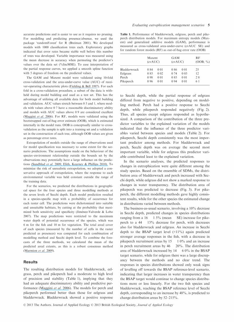
The resulting distribution models for bladderwrack, eel-
grass, perch and pikeperch had a moderate to high level
of precision and stability (Table 1), implying that they
had an adequate discriminatory ability and predictive per-
formance (Maggini et al. 2006). The models for perch and
pikeperch performed better than those for eelgrass and
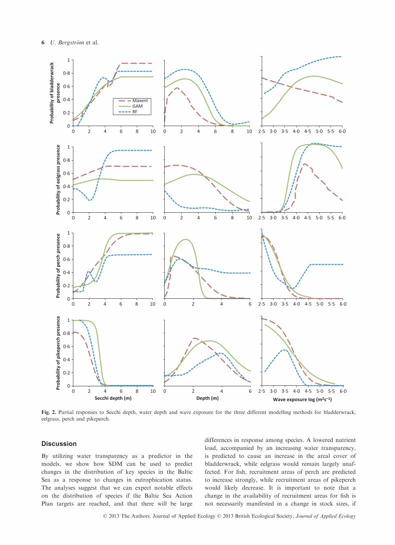
bladderwrack. Bladderwrack showed a positive response
to Secchi depth, while the partial response of eelgrass
differed from negative to positive, depending on model-
ling method. Perch had a positive response to Secchi
depth, while pikeperch responded negatively (Fig. 2).
Thus, all species except eelgrass responded as hypothe-
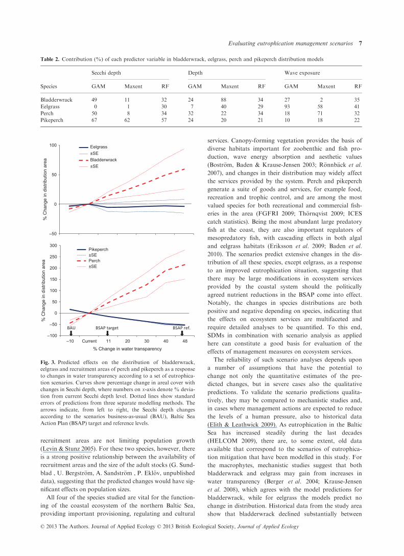
sized. A comparison of the contribution of the three pre-
dictor variables to the explained variation of the models
indicated that the influence of the three predictor vari-
ables varied between species and models (Table 2). For
pikeperch, Secchi depth consistently was the most impor-
tant predictor among methods. For bladderwrack and
perch, Secchi depth was on average the second most
important variable, while for eelgrass this predictor vari-
able contributed least to the explained variation.
In the scenario analyses, the predicted responses to
changes in eutrophication were quite different among the
study species. Based on the ensemble of SDMs, the distri-
bution area of bladderwrack and perch increased with Sec-
chi depth, while eelgrass did not show a marked response to
changes in water transparency. The distribution area of
pikeperch was predicted to decrease (Fig. 3). For pike-
perch, the different modelling methods gave highly consis-
tent results, while for the other species the estimated change
in distributions varied between methods.
The business-as-usual scenario, involving a 10% decrease
in Secchi depth, predicted changes in species distributions
ranging from a 16 � 1�5% (mean � SE) increase for pike-
perch to a 44 � 13% decrease for perch, with decreases
also for bladderwrack and eelgrass. An increase in Secchi
depth to the BSAP target level (+11%) again predicted
stronger average responses in the fish, with a decrease in
pikeperch recruitment areas by 15 � 1�0% and an increase
in perch recruitment areas by 46 � 20%. The distribution
area of bladderwrack increased by 14 � 6�0% in the BSAP
target scenario, while for eelgrass there was a large discrep-
ancy between the methods and no clear trend. The
responses in species distributions showed only weak signs
of levelling off towards the BSAP reference-level scenario,
indicating that larger increases in water transparency than
the BSAP target would continue to change species distribu-
tions more or less linearly. For the two fish species and
bladderwrack, reaching the BSAP reference level of Secchi
depth, corresponding to an increase by 48%, is predicted to
change distribution areas by 52–215%.
Table 1. Performance of bladderwrack, eelgrass, perch and pike-
perch distribution models. For maximum entropy models (Max-
ent) and generalized additive models (GAM), performance is
measured as cross-validated area-under-curve (cvAUC�SE) and
for random forest models (RF) as out-of-bag error rate (OOB)
Maxent
(cvAUC)
GAM
(cvAUC)
RF
(OOB; %)
Bladderwrack 0�84 � 0�01 0�86 � 0�01 25
Eelgrass 0�85 � 0�02 0�74 � 0�03 12
Perch 0�98 � 0�01 0�85 � 0�01 2�8Pikeperch 0�96 � 0�01 0�94 � 0�01 6�1
© 2013 The Authors. Journal of Applied Ecology © 2013 British Ecological Society, Journal of Applied Ecology
Evaluating eutrophication management scenarios 5
Discussion
By utilizing water transparency as a predictor in the
models, we show how SDM can be used to predict
changes in the distribution of key species in the Baltic
Sea as a response to changes in eutrophication status.
The analyses suggest that we can expect notable effects
on the distribution of species if the Baltic Sea Action
Plan targets are reached, and that there will be large
differences in response among species. A lowered nutrient
load, accompanied by an increasing water transparency,
is predicted to cause an increase in the areal cover of
bladderwrack, while eelgrass would remain largely unaf-
fected. For fish, recruitment areas of perch are predicted
to increase strongly, while recruitment areas of pikeperch
would likely decrease. It is important to note that a
change in the availability of recruitment areas for fish is
not necessarily manifested in a change in stock sizes, if
2·5 3·0 3·5 4·0 4·5 5·0 5·5 6·00 2 4 6 8 100
0·2
0·4
0·6
0·8
1
0 2 4 6 8 10
Prob
abili
ty o
f bla
dder
wra
ckpr
esen
cePr
obab
ility
of e
elgr
ass
pres
ence
Prob
abili
ty o
f per
ch p
rese
nce
Prob
abili
ty o
f pik
eper
ch p
rese
nce
MaxentGAMRF
2·5 3·0 3·5 4·0 4·5 5·0 5·5 6·00 2 4 6 8 100
0·2
0·4
0·6
0·8
1
0 2 4 6 8 10
2·5 3·0 3·5 4·0 4·5 5·0 5·5 6·00 2 4 60
0·2
0·4
0·6
0·8
1
0 2 4 6 8 10
2·5 3·0 3·5 4·0 4·5 5·0 5·5 6·0
Wave exposure log (m2s–1)
0 2 4 6Depth (m)
0
0·2
0·4
0·6
0·8
1
0 2 4 6 8 10Secchi depth (m)
Fig. 2. Partial responses to Secchi depth, water depth and wave exposure for the three different modelling methods for bladderwrack,
eelgrass, perch and pikeperch.
© 2013 The Authors. Journal of Applied Ecology © 2013 British Ecological Society, Journal of Applied Ecology
6 U. Bergstr€om et al.
recruitment areas are not limiting population growth
(Levin & Stunz 2005). For these two species, however, there
is a strong positive relationship between the availability of
recruitment areas and the size of the adult stocks (G. Sund-
blad , U. Bergstr€om, A. Sandstr€om , P. Ekl€ov, unpublished
data), suggesting that the predicted changes would have sig-
nificant effects on population sizes.
All four of the species studied are vital for the function-
ing of the coastal ecosystem of the northern Baltic Sea,
providing important provisioning, regulating and cultural
services. Canopy-forming vegetation provides the basis of
diverse habitats important for zoobenthic and fish pro-
duction, wave energy absorption and aesthetic values
(Bostr€om, Baden & Krause-Jensen 2003; R€onnb€ack et al.
2007), and changes in their distribution may widely affect
the services provided by the system. Perch and pikeperch
generate a suite of goods and services, for example food,
recreation and trophic control, and are among the most
valued species for both recreational and commercial fish-
eries in the area (FGFRI 2009; Th€ornqvist 2009; ICES
catch statistics). Being the most abundant large predatory
fish at the coast, they are also important regulators of
mesopredatory fish, with cascading effects in both algal
and eelgrass habitats (Eriksson et al. 2009; Baden et al.
2010). The scenarios predict extensive changes in the dis-
tribution of all these species, except eelgrass, as a response
to an improved eutrophication situation, suggesting that
there may be large modifications in ecosystem services
provided by the coastal system should the politically
agreed nutrient reductions in the BSAP come into effect.
Notably, the changes in species distributions are both
positive and negative depending on species, indicating that
the effects on ecosystem services are multifaceted and
require detailed analyses to be quantified. To this end,
SDMs in combination with scenario analysis as applied
here can constitute a good basis for evaluation of the
effects of management measures on ecosystem services.
The reliability of such scenario analyses depends upon
a number of assumptions that have the potential to
change not only the quantitative estimates of the pre-
dicted changes, but in severe cases also the qualitative
predictions. To validate the scenario predictions qualita-
tively, they may be compared to mechanistic studies and,
in cases where management actions are expected to reduce
the levels of a human pressure, also to historical data
(Elith & Leathwick 2009). As eutrophication in the Baltic
Sea has increased steadily during the last decades
(HELCOM 2009), there are, to some extent, old data
available that correspond to the scenarios of eutrophica-
tion mitigation that have been modelled in this study. For
the macrophytes, mechanistic studies suggest that both
bladderwrack and eelgrass may gain from increases in
water transparency (Berger et al. 2004; Krause-Jensen
et al. 2008), which agrees with the model predictions for
bladderwrack, while for eelgrass the models predict no
change in distribution. Historical data from the study area
show that bladderwrack declined substantially between
Table 2. Contribution (%) of each predictor variable in bladderwrack, eelgrass, perch and pikeperch distribution models
Species
Secchi depth Depth Wave exposure
GAM Maxent RF GAM Maxent RF GAM Maxent RF
Bladderwrack 49 11 32 24 88 34 27 2 35
Eelgrass 0 1 30 7 40 29 93 58 41
Perch 50 8 34 32 22 34 18 71 32
Pikeperch 67 62 57 24 20 21 10 18 22
–50
0
50
100
% C
hang
e in
dis
tribu
tion
area
Eelgrass±SEBladderwrack±SE
–100
–50
0
50
100
150
200
250
300
–10 Current 11 20 30 40 48
% C
hang
e in
dis
tribu
tion
area
% Change in water transparency
Pikeperch±SEPerch±SE
BSAP ref.BSAP targetBAU
Fig. 3. Predicted effects on the distribution of bladderwrack,
eelgrass and recruitment areas of perch and pikeperch as a response
to changes in water transparency according to a set of eutrophica-
tion scenarios. Curves show percentage change in areal cover with
changes in Secchi depth, where numbers on x-axis denote % devia-
tion from current Secchi depth level. Dotted lines show standard
errors of predictions from three separate modelling methods. The
arrows indicate, from left to right, the Secchi depth changes
according to the scenarios business-as-usual (BAU), Baltic Sea
Action Plan (BSAP) target and reference levels.
© 2013 The Authors. Journal of Applied Ecology © 2013 British Ecological Society, Journal of Applied Ecology
Evaluating eutrophication management scenarios 7

the 1940s and the 1980s (Kangas et al. 1982; Kautsky
et al. 1986). For eelgrass, available long-term studies from
the northern Baltic Sea suggest no declines in the distribu-
tion in Finland (Bostr€om et al. 2002) and Estonia (M€oller
& Martin 2007). In the study region, eelgrass distribution
appears to be influenced by a trade-off between light
availability and physical exposure. In contrast to marine
coastal regions, eelgrass in our study area thrives on
exposed sandy sea floor in the outer archipelago areas
with relatively good water transparency (Bostr€om et al.
2006). However, with increasing Secchi depth, exposure
values peak beyond the suitable range for eelgrass, and
the subsequent response in areal distribution remains
weak. The lack of response in eelgrass can also be
explained by other factors, such as stochastic events, com-
petition with freshwater plants in sheltered areas and
availability of suitable sandy substrates, may be more
important in the northern Baltic Sea (Krause-Jensen et al.
2008). Thus, for bladderwrack, the results of our scenario
analyses agree well with current knowledge, while for
eelgrass mechanistic studies and historical data from the
study area are somewhat contradictory. These results
illustrate the potential utility of SDMs for exploring how
the distribution of species suggested as indicators within
the Water Framework Directive and the Marine Strategy
Framework Directive responds to changes in specific
pressures.
The responses of perch and pikeperch are consistent
with knowledge about water transparency preferences for
early life stages of the two species. Perch recruits are
known to gain from a high water transparency, while
young pikeperch is adapted to turbid waters (Sandstr€om
& Kar�as 2002; Ljunggren & Sandstr€om 2007). When com-
paring to historical data, based on commercial catch sta-
tistics and coastal fish monitoring, the picture becomes
more complex. In the commercial fishery, pikeperch
catches increased dramatically from the 1950s to the
1980s, that is, at the onset of eutrophication, while perch
catches decreased several-fold during the same period in
the northern Baltic Sea. These changes probably reflect
the increase in eutrophication status and turbidity (Lehto-
nen 1985; Hansson & Rudstam 1990; Swedish official
catch statistics), in line with our predictions. On the other
hand, fish monitoring data, which are available from the
1980s onwards, point at increases in perch populations in
the study area during the last decades, while pikeperch
populations have been stable or even decreasing. The
development in the last decades is probably the result of
interacting effects of climate change, eutrophication and
fishing (HELCOM 2012; Olsson, Bergstr€om & G�ardmark
2012, N. Mustam€aki , K. �Adjers , U. Bergstr€om, J. Mattila,
unpublished). These dynamics illustrate the complex
nature of population regulation in fish stocks and show
that SDMs incorporating only one pressure variable may
not be successful in predicting the dynamics of popula-
tions. In this study, however, we wanted to test the
hypothesized effects of the politically agreed eutrophica-
tion targets in isolation from other potential changes in
the environment, and as such, the scenario analyses are
still valuable.
Species distribution modelling, and predictions of future
distributions in particular, may be affected by uncertainty
stemming from both the modelling process and the specifi-
cation of scenarios (Coreau et al. 2009; Elith & Leathwick
2009). Quantifying and communicating these uncertainties
is a central part in scenario analysis, as this information is
vital for politicians or managers using the scenarios in deci-
sion-making. For the Baltic Sea, it is difficult to predict
how soon nutrient reduction measures will translate into
alleviated eutrophication symptoms of the Baltic Sea,
including changes in water transparency, and how much
change we can expect, especially as climate-induced changes
will likely counteract these measures (Meier, Eilola &
Almroth 2011). To accommodate for this source of uncer-
tainty, we made predictions of species distributions across a
range of Secchi depths, not only those specified by the sce-
narios. Thereby, we could graphically illustrate how species
respond to Secchi depth. This approach is helpful in the
interpretation of results in cases where the magnitude of
change in the pressure variable is uncertain. These graphs
show that the response to water transparency changes is
predicted to be fairly linear, not levelling off until Secchi
depth approaches the BSAP reference level. This is true also
for a situation with no action taken. If no nutrient reduc-
tions are achieved and Secchi depth continues to decrease,
then a close to linear negative effect can be anticipated in
bladderwrack and perch, and a positive one in pikeperch.
The lack of thresholds and other complex responses sug-
gests that the qualitative conclusions from the analyses are
robust and that the quantitative effects on habitat distribu-
tions will be nearly linearly related to how large improve-
ments in Secchi depth can be reached for these key species
of the northern Baltic Sea. Nevertheless, it is important to
bear in mind that changes in coastal ecosystems as a result
of nutrient reduction have been observed to be nonlinear
with respect to nutrient loads, water transparency and time.
These complex trajectories, which can probably be
explained by concurrent changes in several human pres-
sures (Duarte et al. 2009), are not captured in simplified
models taking into account only one of these pressures.
Apart from the specification of scenarios, uncertainty in
predictions may also arise from data deficiencies and from
the actual modelling process (Elith & Leathwick 2009).
Quantifying these methodological errors inherent in the
sampling and modelling procedure is crucial for measur-
ing and communicating the precision of the predictions to
stakeholders and policy makers. To increase the quantita-
tive predictive ability of the models, it is important to
minimize these sources of error, while to test the stability
of the predictions, sensitivity analyses need to be per-
formed. Sampling uncertainty, which comes from deficient
data sets due to, for example, small sample sizes or unrep-
resentative sampling, was estimated by cross-validation.
The models had a moderate to high level of precision and
© 2013 The Authors. Journal of Applied Ecology © 2013 British Ecological Society, Journal of Applied Ecology
8 U. Bergstr€om et al.
stability (cvAUC 0�74–0�98, OOB 2�8–25%), indicating
that the samples of species occurrence and the predictor
variables used for calibrating the models captured the
major patterns of species–environment relationships of the
complex coastal region. Model uncertainty, that is,
method-specific errors in the description of species–
environment relationships, was assessed by comparing
predictions of three conceptually different modelling tech-
niques. The performance of the methods was comparable,
all three producing useful models for the species. For all
species except pikeperch, there were, however, relatively
large differences in predicted changes in habitat cover
between the methods. In the perch, bladderwrack and eel-
grass models, the partial response to Secchi depth had a
similar shape but varied in importance between models.
Consequently, the span in the predictions between the
methods was large for these species when applied in geo-
graphical space. This can be contrasted to pikeperch, where
both response curve shape and variable contribution of
Secchi depth were comparable between methods, and the
three models produced very consistent estimates of habitat
distributions for the different scenarios. Our experience
thus suggests that relatively small differences in the shape
of the partial response curves, as well as their relative
importance (within method), may increase when they are
applied in a geographical, predictive, context. In line with
previous studies (Ara�ujo & New 2007; Marmion et al.
2009; Mateo et al. 2012), our results highlight the value of
applying an ensemble approach for minimizing model-
specific errors in predictions of species distributions.
Our results provide a good basis for more in-depth analyses
of the potential consequences of eutrophication mitigation
measures taken around the Baltic Sea. By coupling the
effects on the distribution of key species to ecosystem ser-
vices, it may be possible to generate spatially explicit cost-
benefit estimates (Sanchirico & Mumby 2009), which could
add detail to the coarse-scale analyses of the BSAP done so
far (BalticSTERN 2013). SDMs coupled with scenario
analysis thus have a large potential for use as decision
support tools in conservation planning, as they provide a
systematic way of comparing the effects of alternative
policy options and management measures on species and
habitats. This avenue could be highly attractive for manage-
ment, to help bridging the current gap between economy and
ecology in decision-making (R€onnb€ack et al. 2007; Carpen-
ter et al. 2009). Another application of SDMs and prediction
of future species distributions is in the design of marine pro-
tected area networks. By taking into account future changes
in species distributions as a response to an altered environ-
ment, networks may be designed to be resilient to environ-
mental change (Ara�ujo et al. 2004; Mumby et al. 2011). The
MPA network of the northern Baltic Sea is still deficient
(Sundblad, Bergstr€om & Sandstr€om 2011), and in the work
towards making it ecologically coherent, it would be benefi-
cial to incorporate forecasts of species distributions.
In conclusion, we expect that the effects of eutrophica-
tion mitigation on the Baltic Sea coastal ecosystem will be
pronounced, with species-specific responses to improve-
ments in water transparency leading to changes in ecosys-
tem functioning. The politically agreed environmental
targets of the BSAP will require large-scale and costly
actions in the near future, and taxpayers have the right to
know how they might be affected by the measures, as well
as how the alternative of not taking action would affect
them. The most direct experience of changes in the marine
ecosystem will relate to the highly populated coastal zone.
This study provides a step towards analysing the ecologi-
cal and economic consequences of the BSAP eutrophica-
tion objectives for the coastal ecosystem by providing
quantitative estimates of changes in species distributions
in relation to water transparency.
Acknowledgements
The study was performed within the project PREHAB (Spatial prediction
of benthic habitats in the Baltic Sea), financially supported from the Euro-
pean Community’s Seventh Framework Programme (FP/2007-2013) under
grant agreement n° 217246 made with the joint Baltic Sea research and
development programme. Finnish Environment Institute and Svealandsku-
stens kustvattenv�ardsf€orbund are acknowledged for providing water trans-
parency data, and the Nannut project, Mikael von Numers and Suvi
Kivilahti for species distribution data.
References
�Adjers, K., Appelberg, M., Eschbaum, R., Lappalainen, A., Minde, A.,
Repecka, R. & Thoresson, G. (2006) Trends in coastal fish stocks of the
Baltic Sea. Boreal Environment Research, 11, 13–25.Ahtiainen, H. & Vanhatalo, J. (2012) The value of reducing eutrophication
in European marine areas — a Bayesian meta-analysis. Ecological Eco-
nomics, 83, 1–10.Airoldi, L. & Beck, M.W. (2007) Loss, status and trends for coastal mar-
ine habitats of Europe. Oceanography and Marine Biology: An Annual
Review, 45, 345–405.Ara�ujo, M.B. & New, M. (2007) Ensemble forecasting of species distribu-
tions. Trends in Ecology & Evolution, 22, 42–47.Ara�ujo, M.B., Cabeza, M., Thuiller, W., Hannah, L. & Williams, P.H.
(2004) Would climate change drive species out of reserves? An assess-
ment of existing reserve-selection methods. Global Change Biology, 10,
1618–1626.Ara�ujo, M.B., Alagador, D., Cabeza, M., Nogu�es-Bravo, D. & Thuiller,
W. (2011) Climate change threatens European conservation areas. Ecol-
ogy Letters, 14, 484–492.B€ack, S., Kauppila, P., Kangas, P., Ruuskanen, A., Westberg, V., Perus,
J. & R€aike, A. (2006) A biological monitoring programme for the
coastal waters of Finland according to the EU Water Framework
Directive. Environmental Research, Engineering and Management, 4,
6–11.Backer, H., Lepp€anen, J.-M., Brusendorff, A.C., Forsius, K.,
Stankiewicz, M., Mehtonen, J., Pyh€al€a, M., Laamanen, M.,
Paulom€aki, H., Vlasov, N. & Haaranen, T. (2010) HELCOM Baltic
Sea Action Plan – a regional programme of measures for the marine
environment based on the Ecosystem Approach. Marine Pollution
Bulletin, 60, 642–649.BaltiSTERN 2013. The Baltic Sea – Our Common Treasure. Economics of
Saving the Sea. SwAM Report 2013:4, pp. 1–140. Swedish Agency for
Marine and Water Management, Gothenburg, Sweden.
Baden, S., Bostr€om, C., Tobiasson, S., Arponen, H. & Moksnes, P.-O.
(2010) Relative importance of trophic interactions and nutrient
enrichment in seagrass ecosystems: a broad-scale field experiment in
the Baltic-Skagerrak area. Limnology and Oceanography, 55,
1435–1448.Bennett, E.M., Carpenter, S.R., Peterson, G.D., Cumming, G.S., Zurek,
M. & Pingali, P. (2003) Why global scenarios need ecology. Frontiers in
Ecology and the Environment, 1, 322–329.
© 2013 The Authors. Journal of Applied Ecology © 2013 British Ecological Society, Journal of Applied Ecology
Evaluating eutrophication management scenarios 9

Berger, R., Bergstr€om, L., Gran�eli, E. & Kautsky, L. (2004) How does
eutrophication affect different life stages of Fucus vesiculosus in the Bal-
tic Sea? – a conceptual model. Hydrobiologia, 514, 243–248.Bonsdorff, E. & Blomqvist, E.M. (1993) Biotic couplings on shallow water
soft bottoms - examples from the northern Baltic Sea.. Oceanography
and Marine Biology: An Annual Review, 31, 153–176.Bostr€om, C., Baden, S. & Krause-Jensen, D. (2003) The seagrasses of
Scandinavia and the Baltic Sea. World Atlas of Seagrasses: Present Sta-
tus and Future Conservation (eds E.P. Green & F.T. Short), pp. 27–35.University of California Press, Berkeley.
Bostr€om, C., Bonsdorff, E., Kangas, P. & Norkko, A. (2002) Long-term
changes of a brackish-water eelgrass (Zostera marina L.) community
indicate effects of coastal eutrophication. Estuarine, Coastal and Shelf
Science, 55, 795–804.Bostr€om, C., O’Brien, K., Roos, C. & Ekebom, J. (2006) Environmental
variables explaining structural and functional diversity of seagrass mac-
rofauna in an archipelago landscape. Journal of Experimental Marine
Biology and Ecology, 335, 52–73.Breiman, L. (2001) Random forests. Machine Learning, 45, 5–32.Carpenter, S.R., Mooney, H.A., Agard, J., Capistrano, D., DeFries, R.S.,
D�ıaz, S., Dietz, T., Duraiappah, A.K., Oteng-Yeboah, A., Pereira,
H.M., Perrings, C., Reid, W.V., Sarukhan, J., Scholes, R.J. & Whyte,
A. (2009) Science for managing ecosystem services: Beyond the Millen-
nium Ecosystem Assessment. Proceedings of the National Academy of
Sciences, 106, 1305–1312.Cloern, J.E. (2001) Our evolving conceptual model of the coastal eutrophi-
cation problem. Marine Ecology Progress Series, 210, 223–253.Coreau, A., Pinay, G., Thompson, J.D., Cheptou, P.-O. & Mermet, L.
(2009) The rise of research on futures in ecology: rebalancing scenarios
and predictions. Ecology Letters, 12, 1277–1286.Cutler, D.R., Edwards, T.C., Beard, K.H., Cutler, A., Hess, K.T., Gibson,
J. & Lawler, J.J. (2007) Random forests for classification in ecology.
Ecology, 88, 2783–2792.Diaz, R.J. & Rosenberg, R. (2008) Spreading dead zones and conse-
quences for marine ecosystems. Science, 321, 926–929.Duarte, C., Conley, D., Carstensen, J. & S�anchez-Camacho, M. (2009)
Return to Neverland: Shifting baselines affect eutrophication restoration
targets. Estuaries and Coasts, 32, 29–36.Elith, J., Kearney, M. & Phillips, S. (2010) The art of modelling range-
shifting species. Methods in Ecology and Evolution, 1, 330–342.Elith, J. & Leathwick, J.R. (2009) Species distribution models: ecological
explanation and prediction across space and time. Annual Review of
Ecology, Evolution, and Systematics, 40, 677–697.Elith, J., H. Graham, C., P. Anderson, R., Dudik, M., Ferrier, S., Guisan,
A., J. Hijmans, R., Huettmann, F., R. Leathwick, J., Lehmann, A., Li,
J., G. Lohmann, L., A. Loiselle, B., Manion, G., Moritz, C., Nakam-
ura, M., Nakazawa, Y., McC. M. Overton, J., Townsend Peterson, A.,
J. Phillips, S., Richardson, K., Scachetti-Pereira, R., E. Schapire, R.,
Soberon, J., Williams, S., S. Wisz, M. & E. Zimmermann, N. (2006)
Novel methods improve prediction of species’ distributions from occur-
rence data. Ecography, 29, 129–151.Elith, J., Phillips, S.J., Hastie, T., Dud�ık, M., Chee, Y.E. & Yates, C.J.
(2011) A statistical explanation of MaxEnt for ecologists. Diversity and
Distributions, 17, 43–57.Elofsson, K. (2010) Cost-effectiveness of the Baltic Sea Action Plan.
Marine Policy, 34, 1043–1050.Eriksson, B.K. & Bergstr€om, L. (2005) Local distribution patterns of mac-
roalgae in relation to environmental variables in the northern Baltic
Proper. Estuarine, Coastal and Shelf Science, 62, 109–117.Eriksson, B.K., Ljunggren, L., Sandstr€om, A., Johansson, G., Mattila, J.,
Rubach, A., R�aberg, S. & Snickars, M. (2009) Declines in predatory fish
promote bloom-forming macroalgae. Ecological Applications, 19,
1975–1988.FGFRI (2009) Recreational fishing 2008. Official Statistics of Finland –
Agriculture, Forestry and Fishery. URL http://rktl.fi/English/statistics.
Fielding, A.H. & Bell, J.F. (1997) A review of methods for the assessment
of prediction errors in conservation presence/absence models. Environ-
mental Conservation, 24, 38–49.Fleming-Lehtinen, V. & Laamanen, M. (2012) Long-term changes in Secchi
depth and the role of phytoplankton in explaining light attenuation in the
Baltic Sea. Estuarine, Coastal and Shelf Science, 102–103, 1–10.Hansson, S. & Rudstam, L.G. (1990) Eutrophication and Baltic fish com-
munities. AMBIO, 19, 123–125.HELCOM (2007a) HELCOM Baltic Sea Action Plan (adopted by the
HELCOM Ministerial meeting, Krakow, Poland 15th November 2007).
HELCOM (2007b) Outcomes from the Expert Meetings of the HELCOM
Baltic Sea Action Plan, 2.1 Eutrophication Segment. An approach to
set country-wise nutrient reduction allocations to reach good ecological
status of the Baltic Sea. HELCOM HOD 22/2007. Helsinki, HELCOM.
HELCOM (2009) Eutrophication in the Baltic Sea – an integrated the-
matic assessment of the effects of nutrient enrichment in the Baltic Sea
region. Baltic Sea Environment Proceedings, 115B. 1–148. Helsinki Com-
mission, Helsinki, Finland.
HELCOM (2012) Indicator based assessment of coastal fish community
status in the Baltic Sea 2005–2009. Baltic Sea Environment Proceedings,
131. 1–148. Helsinki Commission, Helsinki, Finland.
Isæus, M. (2004) Factors structuring Fucus communities at open and com-
plex coastlines in the Baltic Sea. PhD thesis, Stockholm University.
Jim�enez-Valverde, A. & Lobo, J.M. (2007) Threshold criteria for conver-
sion of probability of species presence to either-or presence-absence.
Acta Oecologia, 31, 361–369.Kangas, P., Autio, H., H€allfors, G., Luther, H., Niemi, �A. & Salemaa, H.
(1982) A general model of the decline of Fucus vesiculosus at Tv€armin-
ne, south coast of Finland in 1977–81. Acta Botanica Fennica, 118,
1–27.Karlsson, O., Jonsson, P., Lindgren, D., Malmaeus, J. & Stehn, A. (2010)
Indications of recovery from hypoxia in the Inner Stockholm Archipel-
ago. AMBIO: A Journal of the Human Environment, 39, 486–495.Kautsky, N., Kautsky, H., Kautsky, U. & Waern, M. (1986) Decreased
depth penetration of Fucus vesiculosus (L.) since the 1940’s indicates
eutrophication of the Baltic Sea. Marine Ecology Progress Series, 28,
1–8.Keith, D.A., Akc�akaya, H.R., Thuiller, W., Midgley, G.F., Pearson, R.G.,
Phillips, S.J., Regan, H.M., Ara�ujo, M.B. & Rebelo, T.G. (2008) Pre-
dicting extinction risks under climate change: coupling stochastic popu-
lation models with dynamic bioclimatic habitat models. Biology Letters,
4, 560–563.Knudby, A., Brenning, A. & LeDrew, E. (2010) New approaches to mod-
elling fish–habitat relationships. Ecological Modelling, 221, 503–511.Korpinen, S., Meski, L., Andersen, J.H. & Laamanen, M. (2012) Human
pressures and their potential impact on the Baltic Sea ecosystem.
Ecological Indicators, 15, 105–114.Krause-Jensen, D., Sagert, S., Schubert, H. & Bostr€om, C. (2008) Empiri-
cal relationships linking distribution and abundance of marine vegeta-
tion to eutrophication. Ecological Indicators, 8, 515–529.Lehtonen, H. (1985) Changes in commercially important freshwater fish
stocks in the Gulf of Finland during recent decades. Finnish Fisheries
Research, 6, 61–70.Lehtonen, H., Hansson, S. & Winkler, H. (1996) Biology and exploitation
of pikeperch, Stizostedion lucioperca (L.), in the Baltic Sea area. Annales
Zologici Fennici, 33, 525–535.Levin, P.S. & Stunz, G.W. (2005) Habitat triage for exploited fishes: Can
we identify essential “Essential Fish Habitat?”. Estuarine, Coastal and
Shelf Science, 64, 70–78.Ljunggren, L. & Sandstr€om, A. (2007) Influence of visual conditions on
foraging and growth of juvenile fishes with dissimilar sensory physiol-
ogy. Journal of Fish Biology, 70, 1319–1334.Maggini, R., Lehmann, A., Zimmerman, N.E. & Guisan, A. (2006)
Improving generalized regression analysis for the spatial prediction of
forest communities. Journal of Biogeography, 33, 1729–1749.Marmion, M., Parviainen, M., Luoto, M., Heikkinen, R.K. & Thuiller,
W. (2009) Evaluation of consensus methods in predictive species distri-
bution modelling. Diversity and Distributions, 15, 59–69.Mateo, R.G., Felicisimo, A.M., Pottier, J., Guisan, A. & Munoz, J. (2012)
Do stacked species distribution models reflect altitudinal diversity pat-
terns? PLoS ONE, 7, e32586.
Meier, H.E.M., Eilola, K. & Almroth, E. (2011) Climate-related changes
in marine ecosystems simulated with a 3-dimensional coupled physi-
cal-biogeochemical model of the Baltic Sea. Climate Research, 48,
31–55.M€oller, T. & Martin, G. (2007) Distribution of the eelgrass Zostera marina
L. in the coastal waters of Estonia, NE Baltic Sea. Proceedings of the
Estonian Academy of Sciences. Biology, Ecology, 56, 270–277.Mumby, P.J., Elliott, I.A., Eakin, C.M., Skirving, W., Paris, C.B.,
Edwards, H.J., Enr�ıquez, S., Iglesias-Prieto, R., Cherubin, L.M. &
Stevens, J.R. (2011) Reserve design for uncertain responses of coral
reefs to climate change. Ecology Letters, 14, 132–140.Olsson, J., Bergstr€om, L. & G�ardmark, A. (2012) Abiotic drivers of
coastal fish community change during four decades in the Baltic Sea.
ICES Journal of Marine Science, 69, 961–970.
© 2013 The Authors. Journal of Applied Ecology © 2013 British Ecological Society, Journal of Applied Ecology
10 U. Bergstr€om et al.
Pereira, H.M., Leadley, P.W., Proenc�a, V., Alkemade, R., Scharlemann,
J.P.W., Fernandez-Manjarr�es, J.F., Ara�ujo, M.B., Balvanera, P., Biggs,
R., Cheung, W.W.L., Chini, L., Cooper, H.D., Gilman, E.L., Gu�enette,
S., Hurtt, G.C., Huntington, H.P., Mace, G.M., Oberdorff, T.,
Revenga, C., Rodrigues, P., Scholes, R.J., Sumaila, U.R. & Walpole,
M. (2010) Scenarios for Global Biodiversity in the 21st Century.
Science, 330, 1496–1501.Phillips, S.J., Anderson, R.P. & Schapire, R.E. (2006) Maximum entropy
modeling of species geographic distributions. Ecological Modelling, 190,
231–259.Phillips, S.J., Dudik, M., Elith, J., Graham, C.H., Lehmann, A., Leath-
wick, J. & Ferrier, S. (2009) Sample selection bias and presence-only
distribution models: implications for background and pseudo-absence
data. Ecological Applications, 19, 181–197.Preisendorfer, R.W. (1986) Secchi disk science: visual optics of natural
waters. Limnology and Oceanography, 31, 909–926.Robinson, L.M., Elith, J., Hobday, A.J., Pearson, R.G., Kendall, B.E.,
Possingham, H.P. & Richardson, A.J. (2011) Pushing the limits in mar-
ine species distribution modelling: lessons from the land present chal-
lenges and opportunities. Global Ecology and Biogeography, 20,
789–802.R€onnb€ack, P., Kautsky, N., Pihl, L., Troell, M., S€oderqvist, T. &
Wennhage, H. (2007) Ecosystem goods and services from swedish
coastal habitats: Identification, valuation, and implications of ecosystem
shifts. Ambio, 36, 534–544.R€onnberg, C. & Bonsdorff, E. (2004) Baltic Sea eutrophication: area-
specific ecological consequences. Hydrobiologia, 514, 227–241.Sanchirico, J. & Mumby, P. (2009) Mapping ecosystem functions to the
valuation of ecosystem services: implications of species–habitat associa-tions for coastal land-use decisions. Theoretical Ecology, 2, 67–77.
Sandman, A., Isæus, M., Bergstr€om, U. & Kautsky, H. (2008) Spatial pre-
dictions of Baltic phytobenthic communities: Measuring robustness of
generalized additive models based on transect data. Journal of Marine
Systems Supplement, 74 (Suppl. 1), S86–S96.Sandstr€om, A. & Kar�as, P. (2002) Effects of eutrophication on young-of-
the-year freshwater fish communities in coastal areas of the Baltic. Envi-
ronmental Biology of Fishes, 63, 89–101.Schories, D., Pehlke, C. & Selig, U. (2009) Depth distributions of Fucus
vesiculosus L. and Zostera marina L. as classification parameters for
implementing the European Water Framework Directive on the German
Baltic coast. Ecological Indicators, 9, 670–680.Sih, A., Jonsson, B.G. & Luikart, G. (2000) Habitat loss: ecological, evo-
lutionary and genetic consequences. Trends in Ecology & Evolution, 15,
132–134.Snickars, M., Sundblad, G., Sandstr€om, A., Ljunggren, L., Bergstr€om,
U., Johansson, G. & Mattila, J. (2010) Habitat selectivity of
substrate-spawning fish: modelling requirements for the Eurasian
perch Perca fluviatilis. Marine Ecology Progress Series, 398, 235–243.Sundblad, G., Bergstr€om, U. & Sandstr€om, A. (2011) Ecological
coherence of marine protected area networks: a spatial assessment
using species distribution models. Journal of Applied Ecology, 48,
112–120.Sundblad, G., H€arm€a, M., Lappalainen, A., Urho, L. & Bergstr€om,
U. (2009) Transferability of predictive fish distribution models in
two coastal systems. Estuarine, Coastal and Shelf Science, 83,
90–96.Th€ornqvist, S. (2009) Fritidsfiskets ut€ovare 2006. Fem studier av fritidsfiske
2002-2007. FINFO 2009:1, pp. 16–62. Swedish Board of Fisheries,
Gothenburg, Sweden.
Veneranta, L., Urho, L., Lappalainen, A. & Kallasvuo, M. (2011) Turbid-
ity characterizes the reproduction areas of pikeperch (Sander lucioperca
(L.)) in the northern Baltic Sea. Estuarine, Coastal and Shelf Science,
95, 199–206.Wikstr€om, S.A. & Kautsky, L. (2007) Structure and diversity of inverte-
brate communities in the presence and absence of canopy-forming Fucus
vesiculosus in the Baltic Sea. Estuarine, Coastal and Shelf Science, 72,
168–176.Wood, S.N. (2006) Generalized Additive Models: An Introduction With R.
Chapman & Hall/CRC. Boca Raton, FL.
Wood, S.N. & Augustin, N.H. (2002) GAMs with integrated model selec-
tion using penalized regression splines and applications to environmen-
tal modelling. Ecological Modelling, 157, 157–177.Wulff, F., Savchuk, O.P., Sokolov, A., Humborg, C. & M€orth, C.-M.
(2007) Management Options and Effects on a Marine Ecosystem:
Assessing the Future of the Baltic. AMBIO: A Journal of the Human
Environment, 36, 243–249.
Received 29 June 2012; accepted 4 March 2013
Handling Editor: David Angeler
Supporting Information
Additional Supporting Information may be found in the online version
of this article.
Appendix S1. Vegetation and fish data sets.
Appendix S2. Construction of a water transparency map as envi-
ronmental background data for the habitat models.
© 2013 The Authors. Journal of Applied Ecology © 2013 British Ecological Society, Journal of Applied Ecology
Evaluating eutrophication management scenarios 11
Copyright © 2022 FDOKUMEN

