Preprint version. Manuscript submitted to the Journal of Medical Imaging Nov 20, 2019

DirectPET: Full Size Neural Network PET Reconstruction fromSinogram Data

William Whiteleya,b,*, Wing K. Lukb, Jens Gregora

aThe University of Tennessee, EECS, 1520 Middle Drive, Knoxville, TN 37996, USAbSiemens Medical Solutions USA Inc., 810 Innovation Drive, Knoxville, TN 37932, USA

Abstract.

Purpose Neural network image reconstruction directly from measurement data is a relatively new field of research,that until now has been limited to producing small single-slice images (e.g., 1x128x128). This paper proposes anovel and more efficient network design for Positron Emission Tomography called DirectPET which is capable ofreconstructing multi-slice image volumes (i.e., 16x400x400) from sinograms.

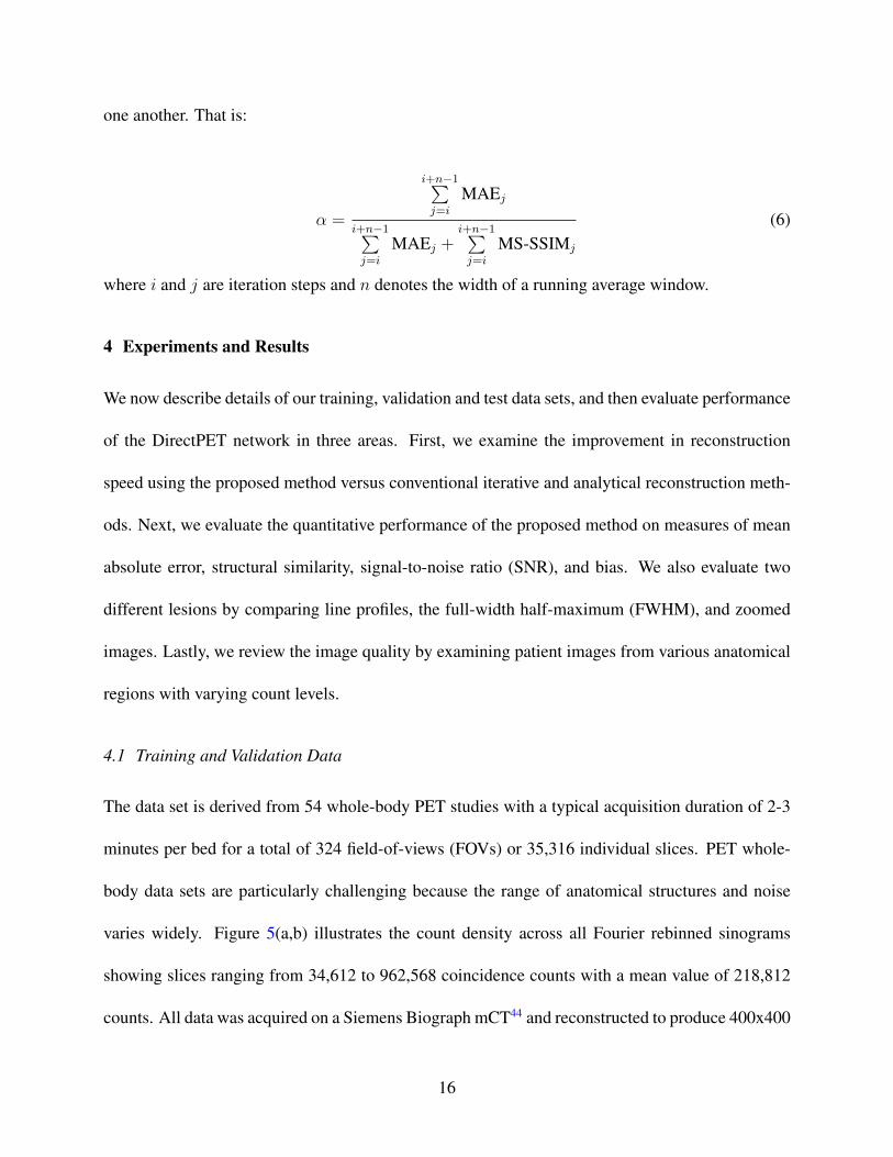
Approach Large-scale direct neural network reconstruction is accomplished by addressing the associated memoryspace challenge through the introduction of a specially designed Radon inversion layer. Using patient data, we comparethe proposed method to the benchmark Ordered Subsets Expectation Maximization (OSEM) algorithm using signal-to-noise ratio, bias, mean absolute error and structural similarity measures. In addition, line profiles and full-widthhalf-maximum measurements are provided for a sample of lesions.

Results DirectPET is shown capable of producing images that are quantitatively and qualitatively similar to theOSEM target images in a fraction of the time. We also report on an experiment where DirectPET is trained to map lowcount raw data to normal count target images demonstrating the method’s ability to maintain image quality under a lowdose scenario.

Conclusion The ability of DirectPET to quickly reconstruct high-quality, multi-slice image volumes suggests po-tential clinical viability of the method. However, design parameters and performance boundaries need to be fullyestablished before adoption can be considered.

Keywords: Image Reconstruction, Medical Imaging, Positron Emission Tomography, Neural Network, Deep Learn-ing.

*William Whiteley, william.whiteley@siemens-healthineers.com

1 Introduction

Reconstructing a medical image by approximating a solution to the so-called ill-posed inverse prob-

lem typically falls into one of three broad categories of reconstruction methods: analytical, iterative

and, more recently, deep learning. While conventional analytical and iterative methods are far more

studied, understood and deployed, the recent effectiveness of deep learning in a variety of domains

1

arX

iv:1

908.

0751

6v4

[ee

ss.I

V]

11

Feb

2020

has raised the question whether neural networks are an effective means to directly solve the in-

verse imaging problem. In this article, we explore an answer to that question for Positron Emission

Tomography (PET) with the development of DirectPET, a deep neural network capable of recon-

structing a multi-slice image volume directly from Radon encoded measurement data. We analyze

the quality of DirectPET reconstructions both qualitatively and quantitatively by comparing against

the standard clinical reconstruction benchmark of Ordered Subsets Expectation Maximization plus

Point Spread Function (OSEM+PSF).1, 2 Additionally, we explore the benefits and limitations in-

herent in direct neural network reconstruction.

As a precondition, it is reasonable to ask whether medical image reconstruction is an appro-

priate application for a neural network. The answer to this question is found in the understanding

that feed-forward neural networks have been proven to be general approximators of continuous

functions with bounded input under the Universal Approximation Theorem.3–5 The nature of PET

imaging makes it such a problem with the implication that a solution can be approximated by a

neural network. This leads us to believe that the study of direct neural network reconstruction is a

worthy pursuit.

We acknowledge that the notion of direct neural network reconstruction may be somewhat con-

troversial. The primary criticism, which the authors freely admit is reasonable, is that it foregoes

decades of imaging physics research as well as the careful development of realistic statistical mod-

els to approximate the system matrix, not to mention corrections for scatter and randoms. Instead of

utilizing these handcrafted approximations, data driven reconstruction solves the inverse problem

by directly learning a mapping between measurement data and images from a large number of ex-

amples (targets) and in turn encodes this mapping into millions or billions of network parameters.

The disadvantage with the method is its black box nature and the current inability to understand

2

and explain the reasoning behind a given set of trained parameters for networks of any significant

size or complexity.

Speaking in favor of direct neural network reconstruction, on the other hand, are distinct and

quantifiable benefits not found with conventional methods. First and foremost, we will show that

direct neural network reconstruction provides good image quality with very high computational

efficiency once training has been completed. Specifically, we show that the DirectPET network

can produce a multi-slice image volume comparable to OSEM+PSF in a fraction of the amount of

time needed by the model-based iterative method. Another benefit is the adaptability and flexibility

that deep learning methods provide in that the output can be tuned to exhibit specific desirable

image characteristics by providing training targets with those same characteristics. In particular,

data driven reconstruction methods can produce high quality images, if data sets containing high

quality image targets are available to train the neural network. We demonstrate this ability by

showing that DirectPET can be trained to learn a mapping from low count sinograms to high count

images. Subsequent reconstruction produces images of a quality that is superior to those produced

by OSEM-PSF.

The proposed DirectPET network advances the applicability of direct neural network recon-

struction. AUTOMAP6 and DeepPET7 have only been shown to produce single-slice 1x128x128

images. AUTOMAP has specifically been critiqued8 for the image size being limited by its large

memory space requirement. For direct methods to be of practical relevance, they must be able

to produce larger image sizes as commonly used in clinical practice. DirectPET was designed

for efficiency, and we demonstrate single forward pass simultaneous reconstruction of multi-slice

16x400x400 image volumes. When batch operations are employed, DirectPET can not only recon-

struct an entire full-size 400x400x400 whole-body PET study, but does so in a little more than one

3

second.

In this paper, the general advantages of direct neural network reconstruction methods and the

specific advancements of the proposed DirectPET network are explored with the specific contribu-

tions being as follows:

1. A novel direct reconstruction neural network design: A three segment architecture capable

of full-size multi-slice reconstruction along with a quantitative and qualitative analysis com-

pared to the conventional reconstruction benchmark of OSEM+PSF.

2. Effective direct reconstruction neural network training techniques: We propose specific tech-

niques (loss function, hyper-parameter selection and learning rate management) not utilized

in previous direct reconstruction methods to achieve efficient learning and high image quality

overcoming the often blurry images produced by neural networks using simple L1 or L2 loss

functions.

3. A path to superior image quality: We demonstrate that the image quality depends less on the

raw data and more on the target images used for training.

4. Challenges and a path to overcoming them: We discuss current challenges and limitations

associated with direct neural network reconstruction and propose a future path to reliably

surmounting these obstacles.

2 Related Work

The terms deep learning and image reconstruction are often used in conjunction to describe a sig-

nificant amount of recent research8 that falls into one of three categories: 1) combination of deep

4

learning with a conventional analytical or statistical method; 2) use of a neural network as a non-

linear post reconstruction filter for denoising and mitigating artifacts; and less commonly 3) use of

a neural network to generate an image directly from raw data. This last category of direct neural

network reconstruction, which forms the largest departure from conventional methods, is the focus

of our work.

Early research was based on networks of fully connected multilayer perceptrons9–12 that yielded

promising results, but only for simple low resolution reconstructions. More recent efforts have

capitalized on the growth of computational resources, especially in the area of Graphical Processing

Units (GPUs), which has led to deep networks capable of direct reconstruction. The AUTOMAP

network6 is a recent example that utilizes multiple fully connected layers followed by a sparse

convolutional encoder-decoder to learn a mapping manifold from measurement space to image

space. AUTOMAP is capable of learning a general solution to the reconstruction inverse problem.

However, the generality is achieved by learning an excessively high number of parameters which

limits its application to fairly small single-slice images (e.g., 1x128x128). DeepPET7 is another

example of direct neural network reconstruction that utilizes an encoder-decoder architecture, but

forgoes any fully connected layers. Instead, this network utilizes convolutional layers to encode the

sinogram input (1x288x269) into a higher dimensional feature vector representation (1024x18x17)

which is then decoded by convolutional layers to produce yet another small single-slice image

(e.g., 1x128x128). While both of these novel methods embody significant advancements in direct

neural network reconstruction, there are several noteworthy differences to the DirectPET network

presented here. As mentioned above, DirectPET is capable of producing multi-slice image volumes

(e.g., 16x400x400). We furthermore train and validate DirectPET on actual raw PET data taken

from patient scans as opposed to using simulated data. Also not done previously, we include the

5

attenuation maps as input to the neural network. Finally, DeepPET was shown to become unstable

at low count densities generating erroneous images,7 a problem not encountered for DirectPET

which exhibits consistent performance across all count densities.

A currently more common application of deep learning in the image formation process is com-

bining a neural network with conventional reconstruction. One method is using an image-to-image

neural network to apply an image-space operator to enhance the post reconstruction output. While

the term ”reconstruction” has been attached to some of these methods, the neural network is not

directly involved in solving the inverse imaging problem, and is more accurately described as a post

reconstruction filter. These learned filters have produced improvements compared to conventional

handcrafted alternatives. In PET imaging, these image-space methods are often applied to low dose

images to produce normal dose equivalents13–15 utilizing U-Net16 or ResNet17 style networks. Sim-

ilarly, these methods are demonstrated to work for X-ray CT on low dose image restoration18 and

limited angle19 applications. Jiao et al.20 increased the reconstruction speed by performing a sim-

ple back-projection of PET data and then utilizing a neural network to reduce the typical streaking

artifacts. Cui et al.21 used a novel unsupervised approach to denoise a low count PET image from

the same patient’s previous high quality image.

As an alternative to the image-space methods, other efforts have included deep learning el-

ements inside the conventional iterative reconstruction process creating unrolled neural network

methods. This often takes the form of using the neural network as a denoising or regularizing op-

erator inside the iterative loop for both PET22, 23 and X-ray CT24, 25 reconstruction. Gong et al.26

replaced the penalty gradient with a neural network in their Expectation Maximization network

(EMnet) and Alder et al.27 replaced the proximal operators in the primal-dual reconstruction algo-

rithm. While the image-space and unrolled deep learning methods all demonstrated improvement

6

over conventional handcrafted alternatives, in addition to now containing a black box component

in the form of a neural network, they continue to carry all of the disadvantages of conventional

reconstruction methods, namely, the complexity of multiple projection and correction components

and a high computational cost. By comparison, direct neural network reconstruction methods are

relatively simple operators with very high computational efficiency once trained.

3 Methods

3.1 Network Architecture Overview

Figure 1 illustrates where the proposed DirectPET network fits in the PET imaging pipeline. Time-

of-flight (TOF) list-mode data is acquired and histogrammed into sinograms. Random correction,

normalization and arc correction are performed on the raw sinogram data in that order. Scatter

and attenuation correction are not applied in the sinogram domain but instead accounted for by

the learned parameters in the DirectPET neural network. Oblique plane sinograms are eliminated

by applying Fourier rebinning,28 and the TOF dimension of the resulting direct plane sinograms

is collapsed. The sinogram data could have been transformed to 2D Non-TOF data in a single

rebinning step,29 but was done in two steps for convenience with readily available software. X-ray

CT data is acquired to create attenuation maps and for later anatomical visualization. A single

forward pass through the DirectPET network of the PET/CT data then produces the desired multi-

slice image volume.

With reference to Figure 2, DirectPET consists of three distinct segments each designed for a

specific purpose. An encoding segment compresses the sinogram data into a lower dimensional

space. A domain transformation segment uses specially designed data masking along with small

fully connected layers to carry out the Radon inversion needed to convert the compressed sinogram

7

Attenuation Maps

PET/CT Scanner

Sum

TO

F Bin

s

Sinogram Preprocessing Steps

Neural Network

Final ImageVolume

3D TOF Sinograms2D Sinograms

TOF

FORE R

ebin

Ran

dom

Cor

rect

ion

Arc

Corr

ection

Nor

mal

izat

ion

(Note: Scatter and attenuation correction are not performed)

Fig 1: The DirectPET imaging pipeline uses TOF Fourier rebinned PET data and X-ray CT basedattenuation maps to generate PET image volumes.

into image-space. Finally, a refinement and scaling segment enhances and upsamples an initial

image estimate to produce the final multi-slice image volume. Together, the segments comprise

an Encoding, Transformation and Refinement and Scaling (ETRS) architecture.30 We proceed by

describing each segment starting with the domain transformation layer, which is what enables the

DirectPET efficiency, followed by the encoder and then the refinement and scaling segment.

Fig 2: The DirectPET reconstruction neural network consists of three distinct segments each witha specific task: (a) the encoding segment is composed of convolutional layers that compress thesinogram input; (b) the domain transformation segment implements Radon inversion by applyingmasks to filter the compressed sinogram data into small fully connected networks for each of anumber of image patches that are then combined to produce an initial image estimate; and (c) therefinement and scaling segment carries out denoising along with attenuation correction and appliessuper-resolution techniques to produce a final full-scale image.

8

3.1.1 Domain Transformation

The computational cost of performing the domain transformation from sinogram to image space

is a key challenge with direct neural network reconstruction. In previous research6, 9–12 this was

typically accomplished through the use of one or more fully connected layers where every input

element is connected to every output element. This results in a multiplicative scaling of the memory

requirements proportional to the size of the input and the number of neurons, i.e., the number of

sinogram bins and the number of image voxels. Figure 3(a,b) illustrates a simple, single layer

reconstruction experiment where each bin in a 200x168 sinogram is connected to every pixel in

a corresponding 200x200 image. After training to convergence using a natural image data set,

examination of the learned activation maps shown in Figure 3(c) reveals that network learned an

approximation to the inverse Radon transform. Along with noting the sinusoidal distribution of

the activation weights, the other key observation is that the majority of weights in the activation

map are near-zero, meaning they do not contribute to the output image and essentially constitute

irrelevant parameters.

Fig 3: A single, fully-connected layer can be trained to learn the distinctive sinusoidal patternassociated with the Radon transform.

With insight from this initial experiment, we designed a more efficient Radon inversion layer

9

to perform the domain transformation. We eliminated network connections that do not contribute

to the output image by creating small fully-connected networks for each patch in the output image

that are only connected to the relevant subset of sinogram data. The activation maps from the initial

simple experiment were used to create a sinogram mask for each patch in the image. Each of these

masks is then independently applied to the compressed sinogram, and the surviving bins are fed to

an independent fully-connected layer connected to the pixels in the relevant image patch. These

patches are then reassembled to create the initial image estimate. When a multi-slice image volume

is reconstructed, the transformation is carried out independently for each slice in the stack, and the

volume is reassembled at output of the segment. The primary design decision for this segment is

selecting the size of the image patch to consider, and is a trade-off between execution speed and

memory consumption. Considering that a downsized sinogram (i.e., 168x200) is the input to the

Radon inversion layer and a half-scale image estimate (i.e., 1x200x200) is the output, on one end

of the spectrum a patch size of a single pixel results in 31,415 fully connected networks (we only

address pixels in the field of view). On the other end of the spectrum, if the patch size equals

the entire image, only a single fully connected network is required, but this choice requires the

maximum 1.055 billion network parameters. We have settled on using 40x40 pixel patches as a

baseline, but have empirically found that patches with 30x30 to 50x50 pixels provide a good trade-

off between speed and memory consumption. Table 1 shows the parameter count as a function

of patch size selection for 168x200 sinograms and 200x200 images. The parameter count for

AUTOMAP and a single fully-connected layer are included for comparison.

Having selected the patch size, the learned activation maps for each pixel in a patch are summed

together. However, the raw activation maps are noisy and applying a simple threshold to generate

a mask includes sinogram bins that should not contribute to a given image patch. The activation

10

Table 1: The selection of patch size is directly related to the required number of parameters in thetransform segment and inversely related to the number of masks and associated networks impactingthe execution speed.

Network Patch Size Input Size Output Size Segment Parameters Number of MasksAUTOMAP na 200 x 168 200 x 200 6,545,920,000 naFully-Connected Layer 200 x 200 200 x 168 200 x 200 1,055,544,000 1Radon Inversion Layer 60 x 60 200 x 168 200 x 200 627,224,400 16Radon Inversion Layer 40 x 40 200 x 168 200 x 200 382,259,200 28Radon Inversion Layer 30 x 30 200 x 168 200 x 200 353,583,000 52Radon Inversion Layer 20 x 20 200 x 168 200 x 200 238,370,400 88Radon Inversion Layer 10 x 10 200 x 168 200 x 200 209,706,900 336

maps are consequently refined using a three step process of Gaussian smoothing to filter high

frequency noise, morphological opening and closing operations to remove noise and fill gaps, and

thresholding using Li’s iterative minimum cross entropy method.31 Figure 4 illustrates the mask

refining process. The resulting size of the learned mask can also be tuned by adjusting the size of

the Gaussian filter (here σ=4) and the morphological structuring element (here a disk of radius 8).

A somewhat simpler approach that generates less memory efficient masks, but achieves comparable

results, would be to create sinogram masks by forward projecting image patches surrounded by a

small buffer.32

Fig 4: The mask creation process begins with summing the raw pixel activation maps for an im-age patch and then undergoes a process of smoothing, morphological opening and closing, andthresholding to produce the final mask.

11

3.1.2 Encoding

Despite the significant efficiency gains achieved in the domain transformation segment, the original

uncompressed sinogram is still too large to process with only modest computational resources. We

initially explored simple bilinear scaling and angular and line of response compression/summing,

but achieved superior performance allowing a convolutional encoder to learn the optimal compres-

sion. The theory and motivation behind this segment is similar to that found in the first half of an

autoencoder33 where the convolutional kernels extract and forward essential information in each

successive layer. Figure 2(a) shows a detailed diagram of the encoding segment illustrating its

architecture and chosen hyper-parameters consisting of three convolutional layers each with 128

3x3 kernels and a Parametric Rectified Linear Unit (PReLU)34 activation function. Spatial down-

sampling is accomplished by the second convolutional layer employing a kernel stride of 2 along

the r sinogram dimension. While we experimented with the axial dimension (number of slices) of

the input between 1 and 32 slices, we ultimately settled on training DirectPET on 16 slices.

3.1.3 Refinement and Scaling

The final neural network segment is responsible for taking the initial image estimate plus the corre-

sponding attenuation maps and removing noise and scaling the image to full size. The attenuation

maps added at this point in the network provide additional image space anatomical information

which significantly boosts the network’s image quality. The refinement and scaling tasks draw on

significant deep learning research in the areas of denoising35 and super-resolution.36 As illustrated

in Figure 2(c), the refinement and scaling segment uses a simple two stage strategy, where each

stage contains convolutional layers followed by a series of ResNet17 blocks that include an overall

skip connection. This strategy is employed first at half spatial resolution and then again at full

12

resolution after a sub-pixel transaxial scaling by a factor of 2 using the PixelShuffle37 technique.

These two sub-segments are followed by a final convolutional layer that outputs the image volume.

All layers in this segment use 64 3x3 convolutional kernels and PReLU activation.

3.2 Neural Network Training

The DirectPET network was implemented with the PyTorch38 deep learning platform and executed

on single and dual Nvidia Titan RTX GPUs. Training occurred over 1,000 epochs with each epoch

having 2,048 samples of sinogram and image target pairs randomly drawn from the training data

in mini-batches of 16. The Adam optimizer39 was used with β1 = 0.5 and β2 = 0.999, which is

similar to traditional stochastic gradient descent but additionally maintains a separate learning rate

for each network parameter. In addition to the optimizer, a cyclic learning rate scheduler40 was

employed that cycles the learning rate between a lower and upper bound with the amplitude of

the cycle decaying exponentially over time towards the lower bound. This type of scheduler aids

training since the periodic raising of the learning rate provides an opportunity for the network to

escape sub-optimal local minimum and traverse saddle points more rapidly.

Based on a triangular wave function, our scheduler was defined as follows for the kth iteration:

η(k) = Λ(k) (ηmax − ηmin) 0.99995n + ηmin (1a)

Λ(k) , 2

∣∣∣∣ k

1000−⌊

k

1000+

1

2

⌋∣∣∣∣ (1b)

To determine appropriate values for the two bounds, an experiment was performed where the

learning rate was slowly increased and plotted against the loss. The results of this study led us to

designate ηmin = 0.5× 10−5 and ηmax = 9.0× 10−5.

13

The loss function is another primary component of neural network training. Previous research41

dedicated to loss functions for image generation and repair suggested a weighted combination of

the element-wise L1 loss, which is an absolute measure, and a multi-scale structural similarity

(MS-SSIM)42 loss, which is a perceptual measure. We extended this idea by eliminating the static

weighting factor and instead developed a dynamically balanced scale factor α between these two

elements. We also added an additional perceptual feature loss component based on a so-called

VGG network.43 The loss between reconstructed image x and target image x was thus made to

consist of three terms, namely:

L(x, x) = β VGG(x, x) + (1− α) MAE(x, x) + α MS-SSIM(x, x) (2)

The VGG loss is based on a convolutional neural network of the same name. Pre-trained on

the large ImageNet data set, which contains millions of natural images, each convolutional layer

of the VGG network is a general image feature extractor; earlier layers extract fine image details

like lines and edges, while deeper layers extract larger semantic features as the image is spatially

down sampled. In our application, the output from the DirectPET network and the target image

are independently input to the VGG network. After the input passes through each of the first

four layers, the output is saved for comparison. The features from the DirectPET image are then

subtracted from the target image features for each of the four VGG layers. The sum of the absolute

value differences forms the VGG loss. That is:

VGG(x, x) =3∑

`=0

|VGG`(x)− VGG`(x)|. (3)

Thus accounting for perceptual differences helps the DirectPET network reconstruct images of

14

higher fidelity than otherwise possible.

The MAE loss denotes the Mean Absolute Error between reconstructed image x and target

image x calculated over all N voxels:

MAE(x, x) =1

N

N−1∑i=0

|xi − xi|. (4)

The MS-SSIM loss measures structural similarity between the two images based on luminance

(denoted lM ), contrast (denoted cj), and structure (denoted sj) components calculated at M scales.

More specifically:

MS-SSIM(x, x) = 1− l(x, x)M∏j=1

cj(x, x)sj(x, x) (5)

where

l(x, x) =2µxµx + C1

µ2x + µ2

x + C1

,

cj(x, x) =2σxσx + C2

σ2x + σ2

x + C2

,

sj(x, x) =σxx + C3

σxσx + C3

.

As usual, µx and µx denote the two image means, and σ2x and σ2

x are the corresponding variances

while σxx is the covariance. The constants are given by C1 =(K1L)2, C2 =(K2L)2, and C3 =C2/2

where L is the dynamic range of values while K1 = 0.01 and K2 = 0.03 are generally accepted

stability constants.

With respect to the weighting of the VGG loss, we used β = 0.5 for all updates. In contrast,

we used a dynamically calculated value for α that trades off the MAE and MS-SSIM losses against

15

one another. That is:

α =

i+n−1∑j=i

MAEj

i+n−1∑j=i

MAEj +i+n−1∑j=i

MS-SSIMj

(6)

where i and j are iteration steps and n denotes the width of a running average window.

4 Experiments and Results

We now describe details of our training, validation and test data sets, and then evaluate performance

of the DirectPET network in three areas. First, we examine the improvement in reconstruction

speed using the proposed method versus conventional iterative and analytical reconstruction meth-

ods. Next, we evaluate the quantitative performance of the proposed method on measures of mean

absolute error, structural similarity, signal-to-noise ratio (SNR), and bias. We also evaluate two

different lesions by comparing line profiles, the full-width half-maximum (FWHM), and zoomed

images. Lastly, we review the image quality by examining patient images from various anatomical

regions with varying count levels.

4.1 Training and Validation Data

The data set is derived from 54 whole-body PET studies with a typical acquisition duration of 2-3

minutes per bed for a total of 324 field-of-views (FOVs) or 35,316 individual slices. PET whole-

body data sets are particularly challenging because the range of anatomical structures and noise

varies widely. Figure 5(a,b) illustrates the count density across all Fourier rebinned sinograms

showing slices ranging from 34,612 to 962,568 coincidence counts with a mean value of 218,812

counts. All data was acquired on a Siemens Biograph mCT44 and reconstructed to produce 400x400

16

image slices using the manufacturer’s standard OSEM+PSF TOF reconstruction with 3 iterations

and 21 subsets including X-ray CT attenuation correction and a 5x5 Gaussian filter. These con-

ventionally reconstructed images constitute the training targets for the DirectPET network with the

goal of producing images of similar quality. At the outset, 14 patients were set aside with 4 going

into a validation set used to evaluate the model during training and 10 patients comprising the test

set only used to evaluate the final model. Although it is common to normalize input and target data

for neural network training, since we are interested in a quantitative reconstruction, the values are

not normalized but instead the input sinograms and target images are scaled by a fixed value to

create average data values closer to 1, which is conducive to stability during neural network train-

ing. With this in mind, sinogram counts were scaled down by a factor of 5 and image voxel Bq/ml

values were scaled down by a factor of 400. During analysis the images were scaled back to their

normal range to perform comparisons in the original units.

4.2 Reconstruction Speed

One of the most pronounced benefits of direct neural network reconstruction is the computational

efficiency of a trained network and the resulting speed up in the subsequent image formation pro-

cess. While a faster reconstruction may not greatly benefit a typical static PET scan, studies where

a large number of reconstructions are required such as dynamic or gated studies with many frames

or gates will see a significant benefit. In these cases, where conventional reconstruction could take

tens of minutes, it would be reduced to tens of seconds. A fast reconstruction would also allow

a radiologist reading a study to rerun the reconstruction multiple times with different parameters

very quickly if desired. Admittedly this would require the training of a plurality of neural networks

to choose from, but we believe this is what will ultimately be required for direct neural network

17

reconstruction similar to the selection of iterations, subsets, filter and scatter correction in conven-

tional reconstruction to produce the most diagnostically desirable image. Additionally, very fast

reconstruction could enable entirely new procedures such as interventional PET where a probe is

marked with a radioactive tracer, or performing radiation or proton therapy tumor ablation in a

single step with real-time patient imaging/positioning and treatment versus the two-step process

common today.

A comparison of reconstruction speed is shown in Figure 5(c) where all three methods start

from the same set of oblique TOF sinograms and end with a final whole-body image volume. The

test was run on all 10 whole-body data sets, and the average time shown for each method refers to

reconstruction of a single FOV (which makes up 109 image slices). We followed standard clinical

protocols. OSEM+PSF TOF reconstruction was based on 21 subsets and 3 iterations. We used

attenuation and scatter correction as well as post-reconstruction smoothing by a 5x5 Gaussian filter.

Filtered Back-Projection (FBP) included the same corrections and filtering. Both reconstructions

were performed on an HP Z8 G4 workstation with two 10-core Intel Xeon Silver 4114 CPUs

running at 2.2 GHz. DirectPET utilized a patch size of 40 x 40 pixels and a batch size of 7. These

reconstructions were performed on an HP Z840 workstation with an Intel E5-2630 CPU running at

2.2 GHz and a single Nvidia Titan RTX GPU.

The results show that reconstruction with the DirectPET image formation pipeline on average

takes 4.3 seconds from start to finish. Is is noteworthy that 3 seconds are dedicated to pre-processing

and the Fourier rebinning while a mere 1.3 seconds is needed for the forward reconstruction pass

of the network. If additional realizations were desired with different reconstruction parameters,

the additional DirectPET reconstructions would only require the 1.3 second forward pass of the

network. In comparison, OSEM+PSF TOF reconstruction of the same data averaged 31 seconds

18

while FBP averaged 21 seconds, which is 7.2x and 4.9x slower respectively.

Fig 5: The histograms in (a) and (b) show the relative distribution of slice counts in the Fourierrebinned sinograms for the training and test sets. (c) Shows the reconstruction time of a singleFOV for both conventional methods and DirectPET demonstrating 7.2x and 4.9x improvementrespectively.

4.3 Quantitative Image Analysis

For this section on quantitative performance and the next section focusing on qualitative aspects,

two versions of DirectPET were trained. The first version, which will be referred to as DirectPET,

was trained using the entire full count PET whole-body training set. The second version, which will

be referred to as DirectPET-50, was trained with half of the raw counts removed using list-mode

thinning while retaining the full count images as training targets. This second network evaluates

the ability of the DirectPET network to produce high quality images from low count input data. For

comparison, the half-count raw data was also reconstructed with OSEM+PSF TOF using the same

reconstruction parameters as the full-count data. Those images are referred to as OSEM+PSF-50.

Figure 6(a) is the measured SNR over an average of 3 VOIs in areas of relative uniform uptake

in the liver for each of the 10 patients in the test set. The DirectPET and DirectPET-50 networks

both exhibit similar but slightly higher SNR values compared with the target OSEM+PSF. This

indicates the neural network produces slightly smoother images with less noise. Smoothing is a

common feature of neural networks due to the data driven way they optimize over a large data

19

set. Smoother images are, of course, only acceptable if structural details are preserved along with

spatial resolution. This is explored below. As one would predict, OSEM+PSF-50 reconstructions

exhibit the lowest SNR indicating a lack of ability to overcome lower count input data.

Bias measurements, which were calculated relative to the target OSEM+PSF images, indicate if

there is an overall mean deviation from the target value. Again these measurements were calculated

from three volumes-of-interest (VOIs) in the liver of each patient and averaged. The results shown

in Figure 6(b) first indicate there is no global systematic bias with the neural network reconstruction

given that about the same amount of positive and negative bias is present across the 10 patients.

The average absolute bias for DirectPET is 1.82% with a maximum of 4.1%. For DirectPET-50 the

average is 2.04% with a maximum of 4.60% . This demonstrates that the neural networks trained

on full and half-counts show similar low biases. Conversely, the OSEM+PSF-50 images have a

negative bias around 50%.

The mean absolute error (MAE) is a common metric in deep learning research to indicate the

accuracy of a trained model and is an explicit component of our loss function. Figure 6(b) shows

the MAE for each patient image volume, again compared to the target OSEM+PSF volume. To

prevent the many zero valued voxels present in the images from skewing the metric, the absolute

difference is only calculated for non-zero voxel values. For DirectPET, the resulting average MAE

value across the 10 data sets is 33.07 Bq/ml. For DirectPET-50 and OSEM+PSF-50, the average

MAE values are 33.57 Bq/ml and 265.7 Bq/ml, respectively. The nearly identical performance of

the two neural networks is driven by MAE being a component of their loss function causing them

to specifically optimize this measurement in the same way.

Defined above, multi-scale structural similarity (MS-SSIM) values range from 0 to 1, where 0

means no similarity whatsoever while 1 means that the images are identical. Figure 6(d) plots MS-

20

Fig 6: Quantitative measurements of the reference OSEM+PSF reconstructions, DirectPET, Di-rectPET trained on half-count input data and OSEM+PSF reconstructed with half-count inputdata show (a) the neural network methods produce images with less noise, (b) introduce a non-systematic bias of less than 5%, (c) produce low absolute voxel error, and (d) produce images thatare perceptually very similar to the target. These plots also show that the neural network trainedwith only half of the raw counts performed about the same as the network trained on full countsfrom a quantitative perspective.

SSIM values for each reconstruction method with full count OSEM+PSF serving as the reference.

DirectPET and DirectPET-50 are seen to achieve similar values with both networks consistently

at or above a value of 0.99 across the 10 data sets. The fact that MS-SSIM is included in the

loss function is what once again leads to similar high performance. By contrast, OSEM+PSF-50

achieves an average structural similarity score of just 0.88.

In Figure 7 we analyze two lesions in two independent images, and compare the benchmark

OSEM+PSF reconstruction to DirectPET, DirectPET-50 and OSEM+PSF-50 reconstructions with

line profiles, measures of full-width half-maximum (FWHM) and zoomed images. While the line

profiles provide some intuition on the neural networks’ performance on spatial resolution, the mea-

surements are from patient data rather than a well defined point source or phantom. Spatial reso-

21

lution can thus only be loosely inferred relative to the reference reconstruction. That is, if spatial

resolution performance is poor, this should be evident in larger FWHM measurements of the neural

network methods compared to the reference. In Figure 7(a) the line profiles between both neural

networks and the reference image are largely overlapping. The FWHM of DirectPET is 0.75%

larger than the reference, DirectPET-50 is 0.98% smaller and OSEM+PSF-50 is 4.9% larger. In

Figure 7(b) a larger lesion is analyzed and in this case the peak of the line profile is distinguishable

between the two neural network methods and the reference, with the DirectPET neural network

achieving a maximum value 6.7% less than the reference and DirectPET-50 14.5% less.

From a qualitative aspect the line profiles, FWHM measurements and zoomed images seem

to indicate reasonable neural network preservation of spatial resolution for this sample of lesions

while also having a slightly higher SNR performance as discussed above. Although the focus of

this paper is primarily on introducing direct neural network reconstruction as a viable method,

the characterization of two randomly selected lesions can best be described as a preliminary and

somewhat anecdotal study. We defer a quantitative examination of a large number of lesions along

with the more well defined procedures of NEMA spatial resolution and image quality to future

work.

4.4 Qualitative Image Image Analysis

In Figure 8 we examine a sampling of 400x400 images slices from various regions of the body con-

taining different count levels, ranging from 330k counts down to 79k counts. We again compare

DirectPET and DirectPET-50 reconstructions to the OSEM+PSF reference. Overall, visual com-

parison indicates strong similarity between the images. In particular, areas of high tracer uptake,

such as the chest in row (a), the lesions in row (b), and the heart in row (c), all show little difference

22

Fig 7: Quantitative analysis of two lesions showing a line profile and full-width half-maximum(FWHM) for each reconstruction method.

to the reference images. Even the lower count images in rows (d) and (e) exhibit nearly identical

areas of high uptake. On close inspection of areas of lower uptake, while still very similar to the

reference, there are minor differences in intensity, structure and blurring present. Whether these

subtle differences are clinically relevant is an open question to be explored in future research on

neural network reconstruction to include lesion detectability, and observer studies.

23

Fig 8: Full resolution test set reconstructions using OSEM+PSF, DirectPET and DirectPET-50methods from a variety of body locations and count levels.

4.5 Limitations and Future Challenges

One long term challenge to direct neural network reconstruction is understanding the boundaries

and limits of a trained network when the quality and content of a medical image is at stake. The data

driven nature of deep learning is both its most powerful strength and greatest weakness. As we and

others have shown, a neural network can, somewhat counter intuitively, take a data set and essen-

tially learn the mapping of physics and geometry of PET image reconstruction despite the inherent

presence of significant noise. On the other hand, there is no mathematical or statistical guarantee

that some unknown new data will be reconstructed with the same image quality. To combat this

uncertainty large carefully curated data sets for training and validation could be maintained that

24

uniformly represent the entire distribution of data a given neural network must learn (ethnicity, age,

physical traits, tracer concentration, disease, etc.). While this someday may be possible, in the near

term a more practical approach is to better understand the boundaries of the network’s underlying

learned distribution and develop techniques to classify or predict the reconstructed quality of previ-

ously unseen data, perhaps again utilizing a neural network for this task, and revert to conventional

reconstruction techniques if the predicted image quality falls below a certain threshold.

There is also the challenge of bootstrapping neural network reconstruction training when a new

scanner geometry, radio-pharmaceutical or other aspect introduces the need to develop a fresh re-

construction (i.e. system matrix and corrections). At the outset of these new developments there

is no data to train the neural network, and so skipping the step of developing conventional recon-

struction methods, at the absolute least to create the data sets for neural network training, is not

practical. It is perhaps possible and even likely to one day create data sets entirely from simulation

that translate into high quality neural network images of patients in the physical world, but this still

remains to be seen.

A more logistical drawback of neural network reconstruction arises if a variety of reconstruction

styles/parameters (attenuation, scatter, filter, noise, etc.) are desired. A single network is likely

insufficient to meet this need, and the solution is to train multiple neural networks each specifically

targeted to produce images with certain characteristics. Although this requires the training and

management of multiple networks, the computational burden can possibly be mitigated through the

use of transfer learning, which accelerates the training of a neural network on a new reconstruction

by starting with a network previously trained on a similar reconstruction.

Regarding comparison with other algorithms, a limitation common to this work and all recent

deep learning medical image reconstruction research is the lack of a robust platform to consistently

25

compare results. Ideally, a large database containing raw data as well as associated state-of-the-

art reconstructions would be publicly available for benchmarking new algorithms. The absence of

such a database combined with the performance sensitivity of neural networks for a given data set in

turn makes it challenging to directly compare the image quality of our method with existing image

space, unrolled network and other direct reconstruction methods, thus limiting the comparison to

differences in approach, computational efficiency and implementation complexity as discussed in

the introduction.

5 Conclusion

We have presented DirectPET, a neural network capable of full size volume PET reconstruction

directly from clinical sinogram data. The network contains three distinct segments, namely, one

for encoding the sinogram data, one for converting the resulting data to image space, and one

for refining and scaling the image for final presentation. The DirectPET network overcomes the

key computational challenge of performing the domain transformation from sinogram to image

space through the use of a novel Radon inversion layer enabling neural network reconstructions

significantly larger (16x400x400) than any previous work. When batch operations are considered,

the reconstruction of an entire PET whole-body scan (e.g., 400x400x400)is possible in a single,

very fast forward pass of the network.

Our work also shows the ability of a neural network to learn a higher quality reconstruction

than the conventional PET benchmark of OSEM+PSF, if provided a training set with superior tar-

get images. This capability was demonstrated by removing half the counts in the raw data through

list-mode thinning, training the DirectPET network to reconstruct full count images from half count

sinogram data, and comparing the results to OSEM+PSF reconstructions on the decimated data.

26

The results showed that the proposed neural network produced images nearly equivalent to using

the full count data and superior to conventional reconstruction of the same data. While DirectPET

was purposefully trained to match the performance of the standard Siemens OSEM+PSF recon-

struction, similarly other suitable techniques such as maximum a posteriori (MAP) reconstruction

or adding a non-local means filter, both of which are known to produce superior images, could have

been used as the neural network training target.

Looking toward future work, there are many possibilities in network architecture, loss functions

and training optimization to explore, which will undoubtedly lead to more efficient reconstructions

and even higher quality images. However, the biggest challenge with producing medical images

is providing overall confidence on neural network reconstruction on unseen samples. While the

understanding of deep learning techniques is growing and becoming less of a black box, future

research should investigate the boundaries and limits of trained neural networks and how they

relate to the underlying data distribution. Additionally, research to understand and quantify the

clinical relevance and impact of neural network generated images will be an important step towards

eventual adoption.

6 Acknowledgements

The authors would like to thank Dr. Michael E. Casey for his advice and feedback, Dr. Chuanyu

Zhou for providing baseline OSEM+PSF reconstruction and Fourier rebinning software, advice and

expertise, and The University of Tennessee Medical Center for providing PET whole-body patient

data.

27

7 Disclosures

No conflicts of interest, financial or otherwise, are declared by the authors. All data was acquired

under the supervision of the institutional review board of The University of Tennessee Medical

Center.

References

1 H. M. Hudson and R. S. Larkin, “Accelerated image reconstruction using ordered subsets of

projection data,” IEEE Transactions on Medical Imaging 13, 601–609 (1994).

2 E. Rapisarda, V. Bettinardi, K. Thielemans, et al., “Image-based point spread function imple-

mentation in a fully 3d OSEM reconstruction algorithm for PET,” Physics in Medicine and

Biology 55, 4131–4151 (2010).

3 K. Hornik, “Approximation capabilities of multilayer feedforward networks,” Neural Netw. 4,

251–257 (1991).

4 B. C. Csji, “Approximation with artificial neural networks,” Master’s thesis, Faculty Sci., Etvs

Lornd Univ., Budapest, Hungary (2001).

5 Z. Lu, H. Pu, F. Wang, et al., “The expressive power of neural networks: A view from the

width,” in Advances in Neural Information Processing Systems 30, I. Guyon, U. V. Luxburg,

S. Bengio, et al., Eds., 6231–6239, Curran Associates, Inc. (2017).

6 B. Zhu, J. Z. Liu, B. R. Rosen, et al., “Image reconstruction by domain-transform manifold

learning,” Nature 555, 487–492 (2018).

7 I. Hggstrm, C. R. Schmidtlein, G. Campanella, et al., “DeepPET: A deep encoderdecoder

network for directly solving the PET image reconstruction inverse problem,” Medical Image

Analysis 54, 253 – 262 (2019).

28

8 G. Wang, J. C. Ye, K. Mueller, et al., “Image reconstruction is a new frontier of machine

learning,” IEEE Transactions on Medical Imaging 37, 1289–1296 (2018).

9 C. E. Floyd, J. E. Bowsher, M. T. Munley, et al., “Artificial neural networks for SPECT

image reconstruction with optimized weighted backprojection,” in Conference Record of the

1991 IEEE Nuclear Science Symposium and Medical Imaging Conference, 2184–2188 vol.3

(1991).

10 A. Bevilacqua, D. Bollini, R. Campanini, et al., “A new approach to Positron Emission To-

mography (PET) image reconstruction using Artificial Neural Networks (ANN),” Interna-

tional Journal of Modern Physics C 9 (2000).

11 P. Paschalis, N. D. Giokaris, A. Karabarbounis, et al., “Tomographic image reconstruction

using Artificial Neural Networks,” Nuclear Instruments and Methods in Physics Research A

527, 211–215 (2004).

12 M. Argyrou, D. Maintas, C. Tsoumpas, et al., “Tomographic image reconstruction based on

artificial neural network (ANN) techniques,” in 2012 IEEE Nuclear Science Symposium and

Medical Imaging Conference Record (NSS/MIC), 3324–3327 (2012).

13 K. Gong, J. Guan, C. Liu, et al., “PET image denoising using a deep neural network through

fine tuning,” IEEE Transactions on Radiation and Plasma Medical Sciences 3, 153–161

(2019).

14 S. J. Kaplan and Y.-M. Zhu, “Full-dose PET image estimation from low-dose PET image

using deep learning: a pilot study,” Journal of Digital Imaging 32, 773–778 (2018).

15 J. Xu, E. Gong, J. Pauly, et al., “200x Low-dose PET Reconstruction using Deep Learning,”

arXiv e-prints , arXiv:1712.04119 (2017).

29

16 O. Ronneberger, P.Fischer, and T. Brox, “U-net: Convolutional networks for biomedical im-

age segmentation,” in Medical Image Computing and Computer-Assisted Intervention (MIC-

CAI), LNCS 9351, 234–241, Springer (2015). (available on arXiv:1505.04597 [cs.CV]).

17 K. He, X. Zhang, S. Ren, et al., “Deep residual learning for image recognition,” in 2016 IEEE

Conference on Computer Vision and Pattern Recognition (CVPR), 770–778 (2016).

18 E. Kang, W. Chang, J. Yoo, et al., “Deep convolutional framelet denosing for low-dose CT via

wavelet residual network,” IEEE Transactions on Medical Imaging 37, 1358–1369 (2018).

19 Y. Han and J. C. Ye, “Framing U-Net via deep convolutional framelets: Application to sparse-

view CT,” IEEE Transactions on Medical Imaging 37, 1418–1429 (2018).

20 J. Jiao and S. Ourselin, “Fast PET reconstruction using Multi-scale Fully Convolutional Neu-

ral Networks,” arXiv e-prints , arXiv:1704.07244 (2017).

21 J. Cui, K. Gong, N. Guo, et al., “PET image denoising using unsupervised deep learning,”

European Journal of Nuclear Medicine and Molecular Imaging (2019).

22 K. Kim, D. Wu, K. Gong, et al., “Penalized PET reconstruction using deep learning prior and

local linear fitting,” IEEE Transactions on Medical Imaging 37, 1478–1487 (2018).

23 K. Gong, J. Guan, K. Kim, et al., “Iterative PET image reconstruction using convolutional

neural network representation,” IEEE Transactions on Medical Imaging 38, 675–685 (2019).

24 B. Chen, K. Xiang, Z. Gong, et al., “Statistical iterative CBCT reconstruction based on neural

network,” IEEE Transactions on Medical Imaging 37, 1511–1521 (2018).

25 L. Gjesteby, Q. Yang, Y. Xi, et al., “Deep learning methods to guide CT image reconstruction

and reduce metal artifacts,” in Medical Imaging 2017: Physics of Medical Imaging, T. G.

30

Flohr, J. Y. Lo, and T. G. Schmidt, Eds., 10132, 752 – 758, International Society for Optics

and Photonics, SPIE (2017).

26 K. Gong, D. Wu, K. Kim, et al., “MAPEM-Net: an unrolled neural network for Fully 3D

PET image reconstruction,” in 15th International Meeting on Fully Three-Dimensional Image

Reconstruction in Radiology and Nuclear Medicine, S. Matej and S. D. Metzler, Eds., 11072,

109 – 113, International Society for Optics and Photonics, SPIE (2019).

27 J. Adler and O. ktem, “Learned primal-dual reconstruction,” IEEE Transactions on Medical

Imaging 37, 1322–1332 (2018).

28 M. Defrise, M. E. Casey, C. Michel, et al., “Fourier rebinning of time-of-flight PET data,”

Physics in Medicine and Biology 50, 2749–2763 (2005).

29 Y. Li, S. Matej, and S. D. Metzler, “A unified fourier theory for time-of-flight PET data,”

Physics in Medicine and Biology 61, 601–624 (2015).

30 W. Whiteley and J. Gregor, “Direct image reconstruction from raw measurement data using an

encoding transform refinement-and-scaling neural network,” in 15th International Meeting on

Fully Three-Dimensional Image Reconstruction in Radiology and Nuclear Medicine, S. Matej

and S. D. Metzler, Eds., 11072, 369 – 373, International Society for Optics and Photonics,

SPIE (2019).

31 C. Li and C. Lee, “Minimum cross entropy thresholding,” Pattern Recognition 26(4), 617 –

625 (1993).

32 W. Whiteley and J. Gregor, “Efficient neural network image reconstruction from raw data us-

ing a radon inversion layer,” in 2019 IEEE Nuclear Science Symposium and Medical Imaging

Conference (NSS/MIC), 1–2 (2019).

31

33 D. E. Rumelhart, G. E. Hinton, and R. J. Williams, “Parallel distributed processing: Explo-

rations in the microstructure of cognition, vol. 1,” in Parallel Distributed Processing, D. E.

Rumelhart, J. L. McClelland, and C. PDP Research Group, Eds., ch. Learning Internal Rep-

resentations by Error Propagation, 318–362, MIT Press, Cambridge, MA, USA (1986).

34 K. He, X. Zhang, S. Ren, et al., “Delving deep into rectifiers: Surpassing human-level perfor-

mance on imagenet classification,” in Proceedings of the 2015 IEEE International Conference

on Computer Vision (ICCV), ICCV ’15, 1026–1034, IEEE Computer Society, (Washington,

DC, USA) (2015).

35 C. Tian, Y. Xu, L. Fei, et al., “Deep learning for image denoising: A survey,” in Genetic

and Evolutionary Computing, J.-S. Pan, J. C.-W. Lin, B. Sui, et al., Eds., 563–572, Springer

Singapore, (Singapore) (2019).

36 W. Yang, X. Zhang, Y. Tian, et al., “Deep learning for single image super-resolution: A brief

review,” IEEE Transactions on Multimedia 21, 1–1 (2019).

37 W. Shi, J. Caballero, F. Huszar, et al., “Real-time single image and video super-resolution us-

ing an efficient sub-pixel convolutional neural network,” 2016 IEEE Conference on Computer

Vision and Pattern Recognition (CVPR) , 1874–1883 (2016).

38 A. Paszke, S. Gross, S. Chintala, et al., “Automatic differentiation in PyTorch,” in NIPS-W,

(2017).

39 D. P. Kingma and J. Ba, “Adam: A method for stochastic optimization,” International Con-

ference on Learning Representations ICLR(’14) (2014).

40 L. N. Smith, “Cyclical learning rates for training neural networks,” 2017 IEEE Winter Con-

ference on Applications of Computer Vision (WACV) , 464–472 (2015).

32

41 H. Zhao, O. Gallo, I. Frosio, et al., “Loss functions for image restoration with neural net-

works,” IEEE Transactions on Computational Imaging 3, 47–57 (2017).

42 Z. Wang, A. C. Bovik, H. R. Sheikh, et al., “Image quality assessment: from error visibility

to structural similarity,” IEEE Transactions on Image Processing 13, 600–612 (2004).

43 K. Simonyan and A. Zisserman, “Very Deep Convolutional Networks for Large-Scale Image

Recognition,” arXiv e-prints , arXiv:1409.1556 (2014).

44 I. Rausch, J. Cal-Gonzalez, D. Dapra, et al., “Performance evaluation of the biograph mct

flow pet/ct system according to the nema nu2-2012 standard,” EJNMMI physics 2, 26 (2015).

William Whiteley is a Director of Software Engineering at Siemens Medical Solutions USA,

Inc. working in molecular imaging and a PhD student at The University of Tennessee, Knoxville

studying artificial intelligence and image reconstruction. He received his BSEE degree from Van-

derbilt University, Nashville, TN and his MSEE degree from Stanford University, Stanford, CA.

His research interests include artificial intelligence, deep learning, medical imaging, and data min-

ing.

Wing K Luk is a senior staff physicist with Siemens Medical Solutions USA, Inc. He received

his BS degree in Engineering, MS degree in Physics and MS degree in Computer Science from

University of Tennessee, Knoxville. His current research interests include PET image reconstruc-

tion, NUMA memory access optimization, dynamic imaging run-time load balancing and AI image

reconstruction.

Dr. Jens Gregor received his PhD in Electrical Engineering from Aalborg University Denmark,

in 1991. He then joined the faculty at the University of Tennessee, Knoxville, where he currently

holds the position of Professor and Associate Department Head in the Department of Electrical

33

Engineering and Computer Science. His research has covered different imaging modalities includ-

ing X-ray and neutron CT, SPECT, and PET with applications ranging from industrial and security

imaging to preclinical and clinical imaging.

34

8 Figure Captions

Figure 1. The DirectPET imaging pipeline uses TOF Fourier rebinned PET data and X-ray CT

based attenuation maps to generate PET image volumes.

Figure 2. The DirectPET reconstruction neural network consists of three distinct segments each

with a specific task: (a) the encoding segment is composed of convolutional layers that compress the

sinogram input; (b) the domain transformation segment implements Radon inversion by applying

masks to filter the compressed sinogram data into small fully connected networks for each of a

number of image patches that are then combined to produce an initial image estimate; and (c) the

refinement and scaling segment carries out denoising along with attenuation correction and applies

super-resolution techniques to produce a final full-scale image.

Figure 3. A single, fully-connected layer can be trained to learn the distinctive sinusoidal pattern

associated with the Radon transform.

Figure 4. The mask creation process begins with summing the raw pixel activation maps for an

image patch and then undergoes a process of smoothing, morphological opening and closing, and

thresholding to produce the final mask.

Figure 5. The histograms in (a) and (b) show the relative distribution of slice counts in the Fourier

rebinned sinograms for the training and test sets. (c) Shows the reconstruction time of a single

FOV for both conventional methods and DirectPET demonstrating 7.2x and 4.9x improvement

respectively.

35

Figure 6. Quantitative measurements of the reference OSEM+PSF reconstructions, DirectPET,

DirectPET trained on half-count input data and OSEM+PSF reconstructed with half-count input

data show (a) the neural network methods produce images with less noise, (b) introduce a non-

systematic bias of less than 5%, (c) produce low absolute voxel error, and (d) produce images that

are perceptually very similar to the target. These plots also show that the neural network trained

with only half of the raw counts performed about the same as the network trained on full counts

from a quantitative perspective.

Figure 7. Quantitative analysis of two lesions showing a line profile and full-width half-maximum

(FWHM) for each reconstruction method.

Figure 8. Full resolution test set reconstructions using OSEM+PSF, DirectPET and DirectPET-50

methods from a variety of body locations and count levels.

36