


Bahasa
Halaman
Hukum

Cost Minimization for Hot Gas Defrost System
A Thesis
Presented to
The Faculty of California Polytechnic State University,
San Luis Obispo
In Partial Fulfillment
Of the Requirements for the Degree
Master of Science in Mechanical Engineering
By:
Jarubutr Dansilasirithavorn
June 2009
ii
© 2009
Jarubutr Dansilasirithavorn
ALL RIGHTS RESERVED
iii
COMMITTEE MEMBERSHIP
TITLE: Cost Minimization for Hot Gas Defrost System
AUTHOR: Jarubutr Dansilasirithavorn
DATE SUMMITED: June 2009
COMMITTEE CHAIR: Jesse Maddren, Ph.D., P.E.
Associate Professor
Department of Mechanical Engineering
Cal Poly, San Luis Obispo
COMMITTEE MEMBER: Glen Thorncroft, Ph.D.
Associate Chair
Department of Mechanical Engineering
Cal Poly, San Luis Obispo
COMMITTEE MEMBER: Andrew Kean, Ph.D.
Assistant Professor
Department of Mechanical Engineering
Cal Poly, San Luis Obispo
iv
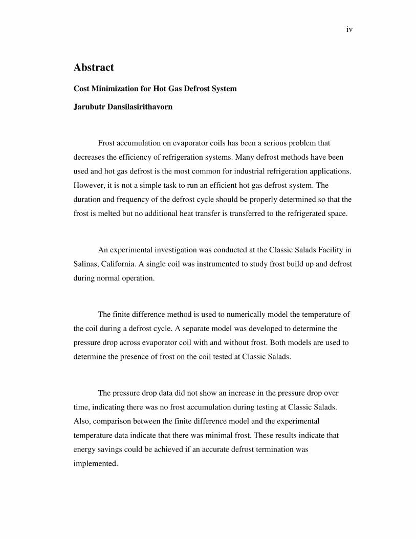
Abstract
Cost Minimization for Hot Gas Defrost System
Jarubutr Dansilasirithavorn
Frost accumulation on evaporator coils has been a serious problem that
decreases the efficiency of refrigeration systems. Many defrost methods have been
used and hot gas defrost is the most common for industrial refrigeration applications.
However, it is not a simple task to run an efficient hot gas defrost system. The
duration and frequency of the defrost cycle should be properly determined so that the
frost is melted but no additional heat transfer is transferred to the refrigerated space.
An experimental investigation was conducted at the Classic Salads Facility in
Salinas, California. A single coil was instrumented to study frost build up and defrost
during normal operation.
The finite difference method is used to numerically model the temperature of
the coil during a defrost cycle. A separate model was developed to determine the
pressure drop across evaporator coil with and without frost. Both models are used to
determine the presence of frost on the coil tested at Classic Salads.
The pressure drop data did not show an increase in the pressure drop over
time, indicating there was no frost accumulation during testing at Classic Salads.
Also, comparison between the finite difference model and the experimental
temperature data indicate that there was minimal frost. These results indicate that
energy savings could be achieved if an accurate defrost termination was
implemented.
v
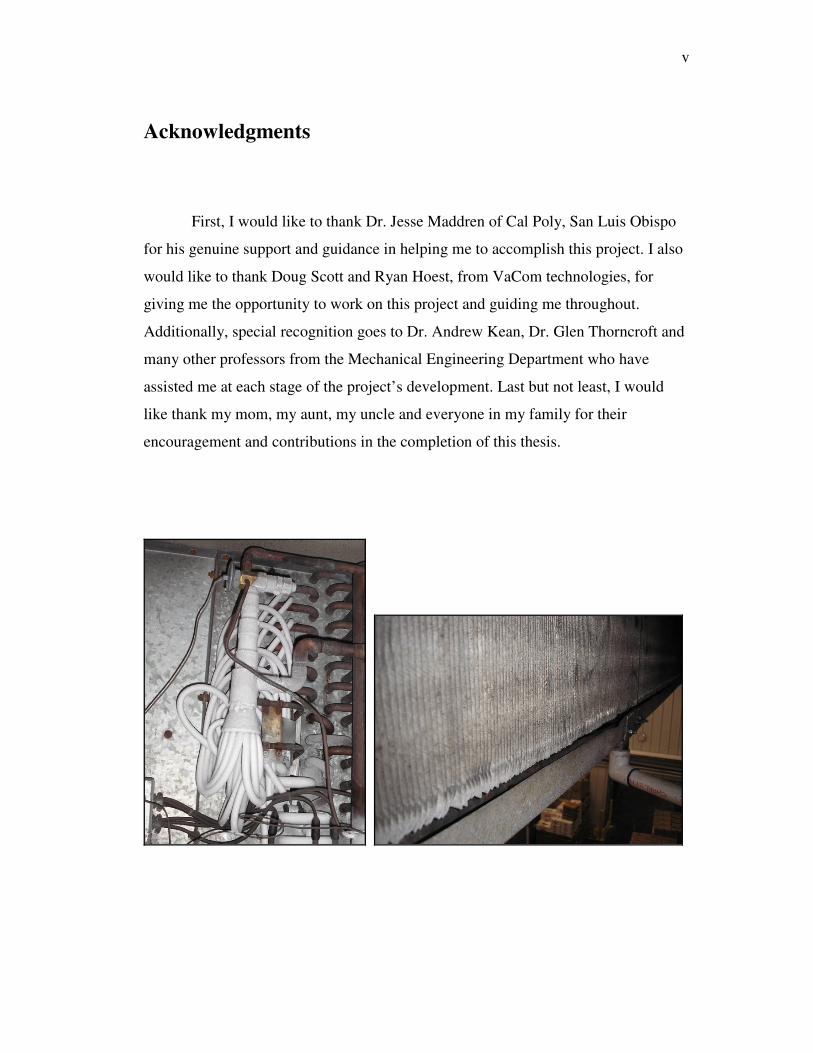
Acknowledgments
First, I would like to thank Dr. Jesse Maddren of Cal Poly, San Luis Obispo
for his genuine support and guidance in helping me to accomplish this project. I also
would like to thank Doug Scott and Ryan Hoest, from VaCom technologies, for
giving me the opportunity to work on this project and guiding me throughout.
Additionally, special recognition goes to Dr. Andrew Kean, Dr. Glen Thorncroft and
many other professors from the Mechanical Engineering Department who have
assisted me at each stage of the project’s development. Last but not least, I would
like thank my mom, my aunt, my uncle and everyone in my family for their
encouragement and contributions in the completion of this thesis.
vi
Table of Contents
List of Figures ...........................................................................................................viii
List of Tables ............................................................................................................... x
Introduction.................................................................................................................. 1
Background .................................................................................................................. 4
Frost ......................................................................................................................... 4
Hot Gas Defrost ....................................................................................................... 5
Literature Review..................................................................................................... 8
Temperature Model.................................................................................................... 11
Pressure Drop Model ................................................................................................. 17
Testing........................................................................................................................ 21
Collecting Data .......................................................................................................... 22
Opto system ........................................................................................................... 22
HOBO System ....................................................................................................... 22
Time Constant........................................................................................................ 24
Results........................................................................................................................ 28
Temperature ........................................................................................................... 28
Pressure drop.......................................................................................................... 34
Efficiency and Cost................................................................................................ 38
Conclusions & Recommendations............................................................................. 42
References.................................................................................................................. 45
Appendix A: LRC evaporator specifications............................................................. 48
Appendix B: Opto22 system and ICTD temperature probe specifications................ 52
vii
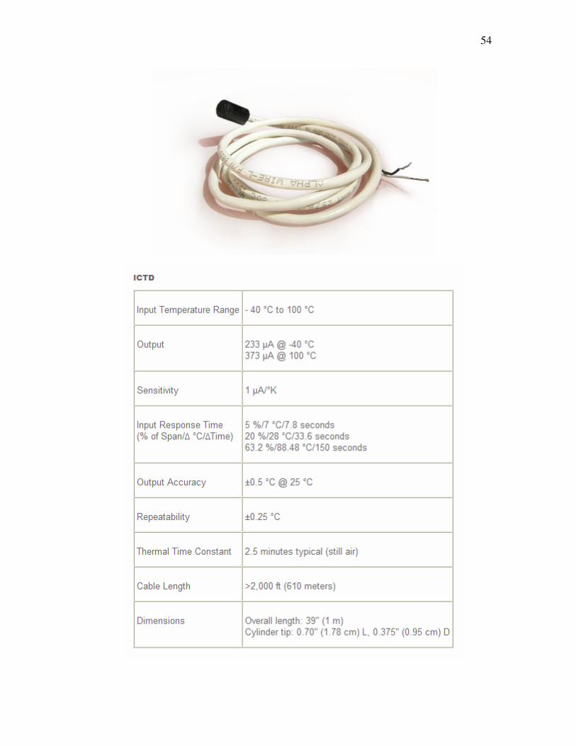
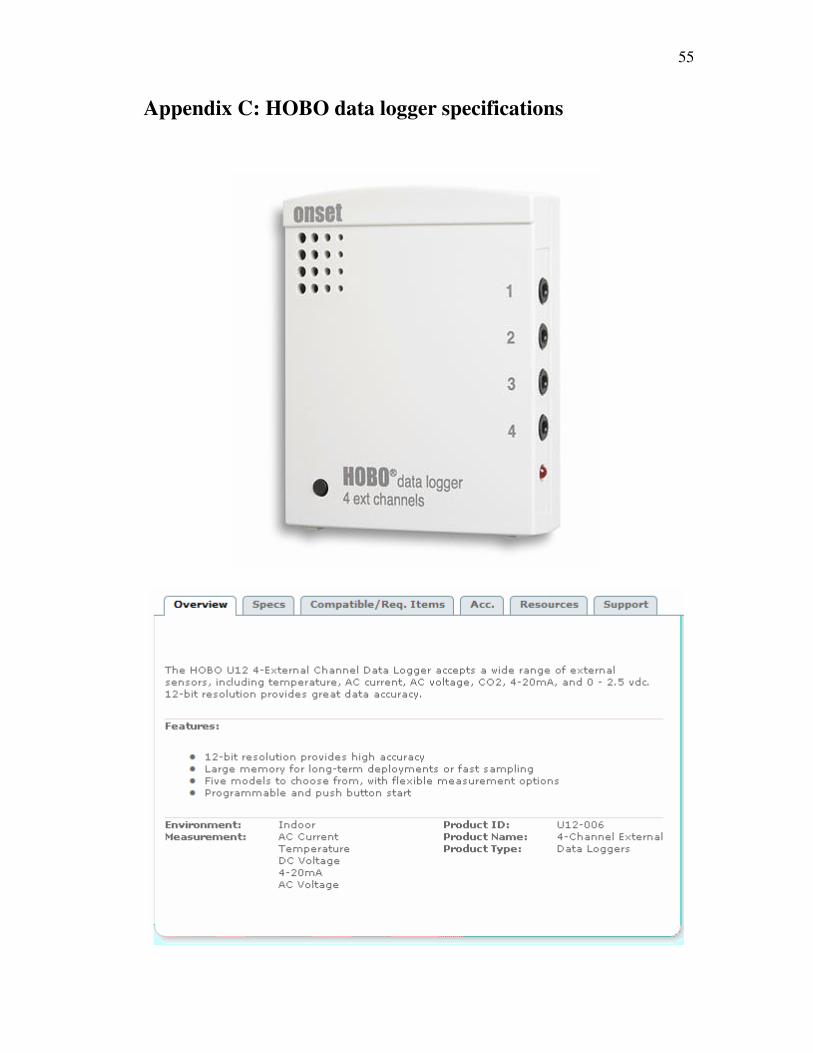
Appendix C: HOBO data logger specifications......................................................... 55
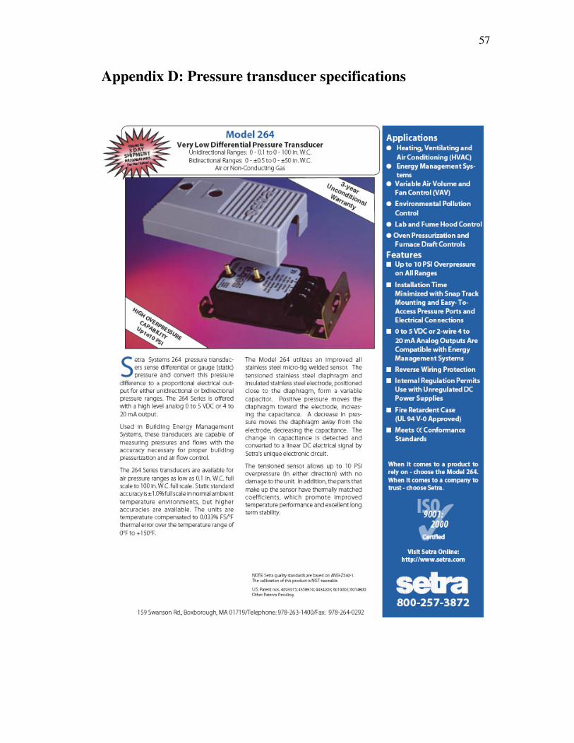
Appendix D: Pressure transducer specifications........................................................ 57
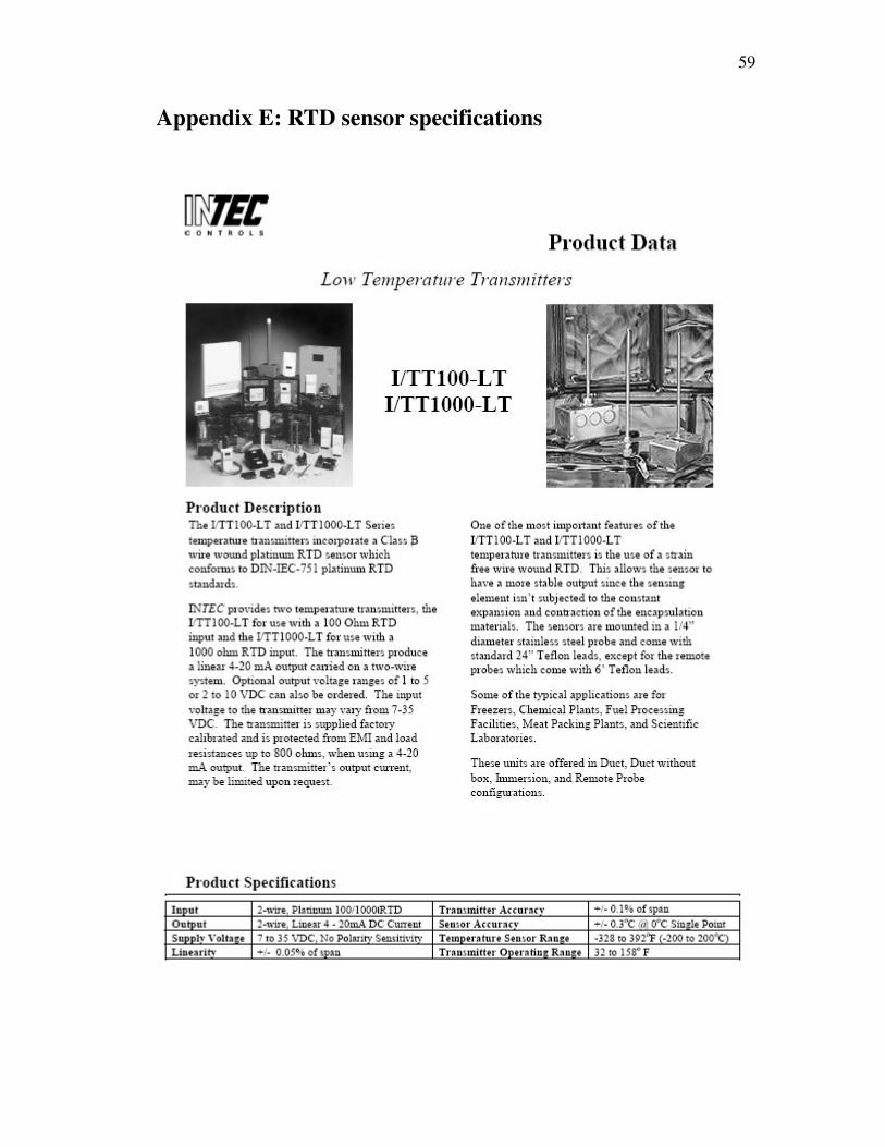
Appendix E: RTD sensor specifications .................................................................... 59
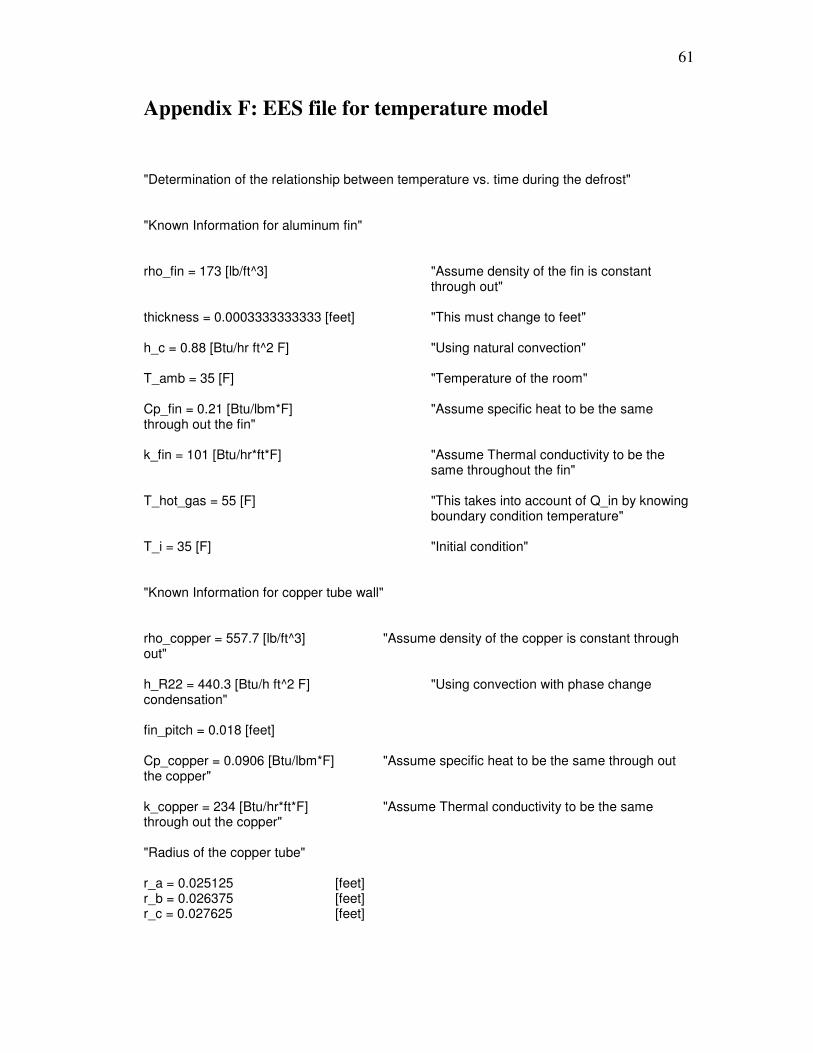
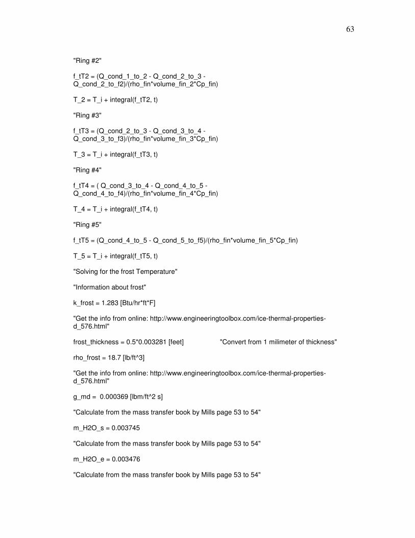
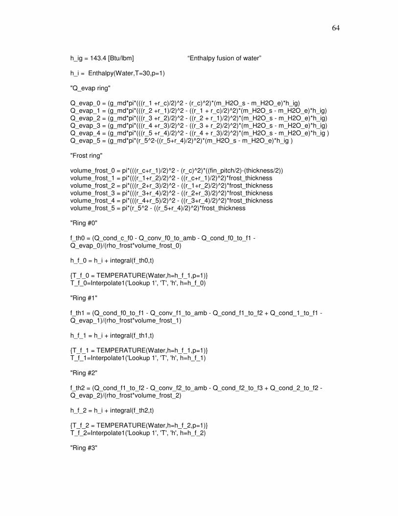
Appendix F: EES file for temperature model ............................................................ 61
Appendix G: EES file for pressure drop model ......................................................... 69
Appendix H: Weather data during experiment .......................................................... 71
viii
List of Figures
Figure 1: Layout of Classic Salads facility .................................................................. 2
Figure 2: Refrigeration unit with hot gas defrost arrangement.................................... 5
Figure 3: Representation of a fin-tube section for a plate-fin heat exchanger........... 11
Figure 4: Schematic of the domain for fin-tube section ............................................ 12
Figure 5: Isometric view with staggered arrangement............................................... 18
Figure 6: Friction factor tubef for staggered tube bundle arrangement ..................... 19
Figure 7: The evaporator inside the Organic Room that was tested .......................... 21
Figure 8: HOBO data recorder for temperature sensors and pressure transducer ..... 23
Figure 9: Temperature data to determine sensor time constant ................................. 25
Figure 10: Location of the RTD inserted between two fins....................................... 26
Figure 11: Locations of RTD on evaporator tube sheet............................................. 27
Figure 12: Temperature data from Opto22 and HOBO systems during the defrost
cycle ........................................................................................................................... 28
Figure 13: Comparison between temperature data and model................................... 30
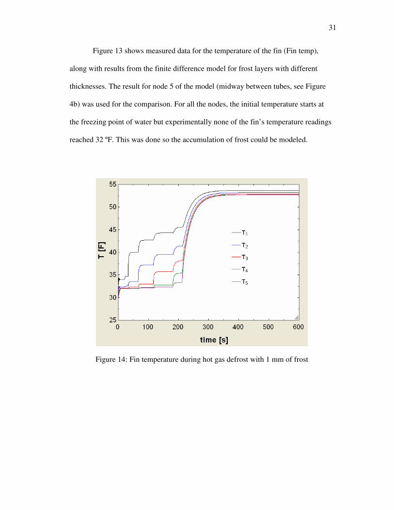
Figure 14: Fin temperature during hot gas defrost with 1 mm of frost...................... 31
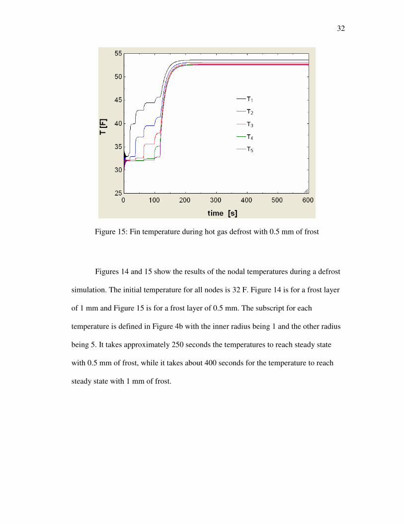
Figure 15: Fin temperature during hot gas defrost with 0.5 mm of frost................... 32
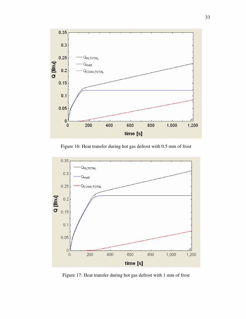
Figure 16: Heat transfer during hot gas defrost with 0.5 mm of frost ....................... 33
Figure 17: Heat transfer during hot gas defrost with 1 mm of frost .......................... 33
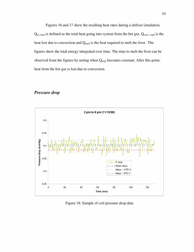
Figure 18: Sample of coil pressure drop data ............................................................ 34
Figure 19: Pressure drop as a function of volumetric flow rate................................. 35
Figure 20: Pressure drop as a function of volumetric flow rate for different frost
thicknesses ................................................................................................................. 36
ix
Figure 21: Pressure drop as a function of volumetric flow rate for different frost
thicknesses and different fan speeds .......................................................................... 37
Figure 22: Hot gas defrost efficiency as a function of defrost time for different
frost thickness ............................................................................................................ 39
Figure 23: Hot gas defrost cost as a function of defrost time for different frost
thickness..................................................................................................................... 41
x
List of Tables
Table 1: Temperature probe specifications for HOBO and Opto systems ................ 24
Table 2: Pressure transducer specifications ............................................................... 24
Table 3: Evaporator coil flow rate and pressure drop as a function of frost
thickness..................................................................................................................... 37
xi
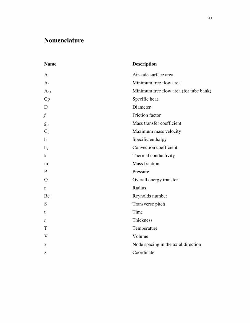
Nomenclature
Name Description
A Air-side surface area
Ac Minimum free flow area
Ac,t Minimum free flow area (for tube bank)
Cp Specific heat
D Diameter
f Friction factor
gm Mass transfer coefficient
Gc Maximum mass velocity
h Specific enthalpy
hc Convection coefficient
k Thermal conductivity
m Mass fraction
P Pressure
Q Overall energy transfer
r Radius
Re Reynolds number
ST Transverse pitch
t Time
t Thickness
T Temperature
V Volume
x Node spacing in the axial direction
z Coordinate
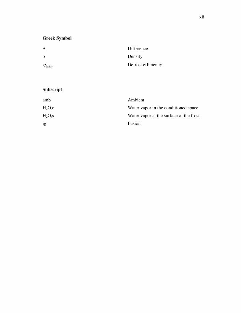
xii
Greek Symbol
∆ Difference
ρ Density
defrostη Defrost efficiency
Subscript
amb Ambient
H2O,e Water vapor in the conditioned space
H2O,s Water vapor at the surface of the frost
ig Fusion
1
Introduction
VaCom Technologies is a consulting refrigeration controls company with
headquarters in Laverne, CA. They also have an office in San Luis Obispo, CA.
They design and install control systems to reduce energy consumption for industrial
refrigeration facilities. One of their clients is Classic Salads located in Salinas, CA.
The Classic Salads facility was recently retrofitted with new energy saving systems
such as variable speed drives on the evaporator coils and floating head pressure
control on the condenser. Nevertheless, VaCom Technologies is still interested in
reducing energy expense by minimizing the defrost frequency and duration. Due to
company workloads and the complexity of this problem, VaCom Technologies
contacted Cal Poly for assistance.
The system at Classic Salads is a single stage R22 refrigeration system with
four Carrier 5H80 reciprocating compressors and one Frick RWBII-134 screw
compressor. There are a total of 26 evaporators, with groups of 2 or 3 in each zone,
as shown in Figure 1. There are 6 auxiliary coils, 3 in the Finished Product room and
3 in the Raw Product room, while the rest are direct expansion coils. All of the
evaporators are defrosted with hot gas refrigerant except the 6 auxiliary coils which
use air to defrost.
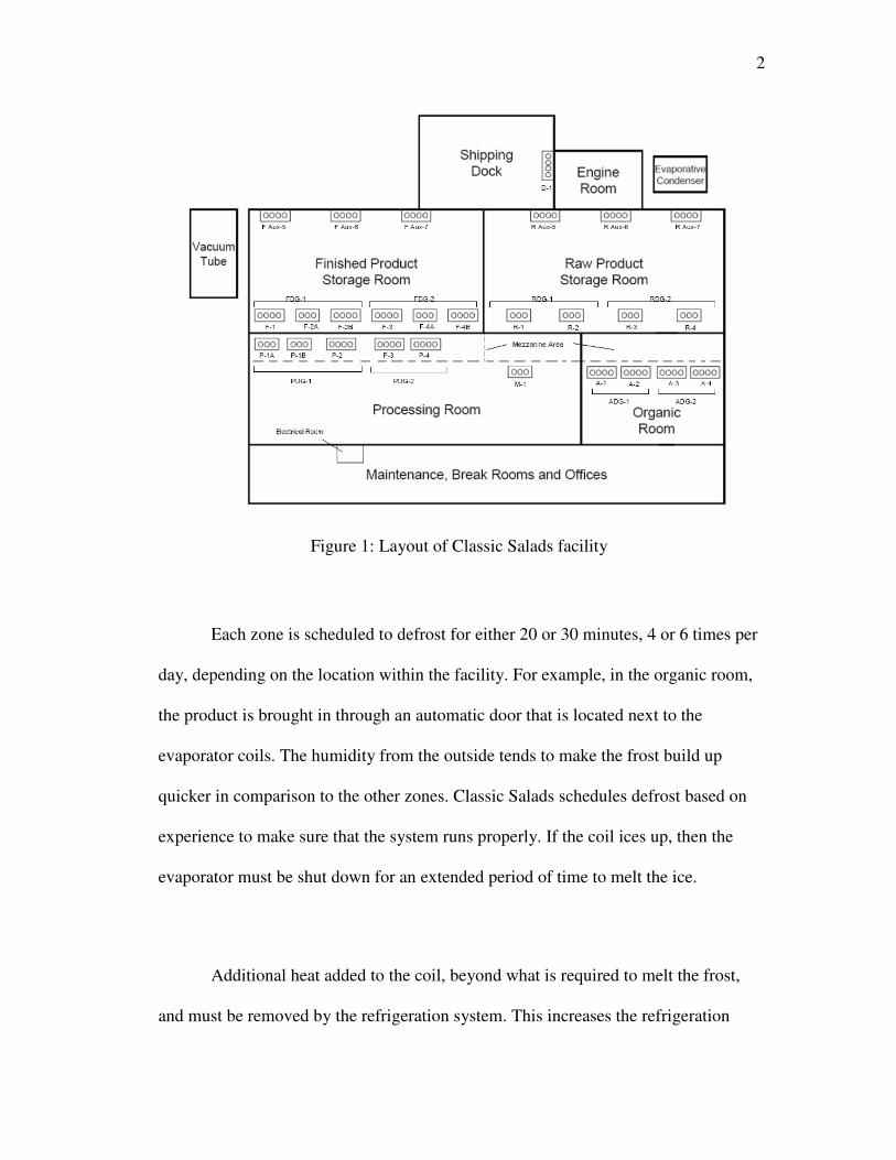
2
Figure 1: Layout of Classic Salads facility
Each zone is scheduled to defrost for either 20 or 30 minutes, 4 or 6 times per
day, depending on the location within the facility. For example, in the organic room,
the product is brought in through an automatic door that is located next to the
evaporator coils. The humidity from the outside tends to make the frost build up
quicker in comparison to the other zones. Classic Salads schedules defrost based on
experience to make sure that the system runs properly. If the coil ices up, then the
evaporator must be shut down for an extended period of time to melt the ice.
Additional heat added to the coil, beyond what is required to melt the frost,
and must be removed by the refrigeration system. This increases the refrigeration
3
load and also the cost of operating the system. The objective of this study is to
determine when to initiate and/or terminate the defrost cycle. If the defrost time is
too short then there will be some frost remaining on the coil when the normal
operation resumes. Energy will be wasted if the defrost time is too long.
Due to limited time and resources, the experimental investigation is limited to
the study of a single coil for a 1 week period. Results from the experiments will be
composed to mathematical models of the coil.
4
Background
Refrigeration is the process of removing heat from a space or a substance and
rejecting it to the surroundings. The main goal of this process is to lower the
temperature of a space or a substance. Refrigeration has been used in wide a range of
applications from air conditioning to food preservation. One of the key components
of the refrigeration system is the evaporator. In food storage applications, the
evaporator sometimes operates below freezing temperature (<32 ºF) and frost can
accumulate on the coil.
Frost
Frost accumulation will occur when the surfaces of the operating evaporative
coil are below 32 ºF and the entering air dew point temperature is higher than the coil
surface temperature [1]. There is a special case when moisture in the air condenses to
liquid water and then freezes to ice. Although, normally the water vapor will
transform directly into a solid phase, frost.
There are two major concerns when the frost formation occurs. First, when
the frost layers grow, the air passages of the evaporator are narrowed. This will
increase the resistance to the air flow. This frost layer will reduce the ability of the
evaporator fan to move air through the coil and fan energy consumption will
increase. Second, frost accumulation increases the resistance to heat transfer due to
5
the low conductivity of the frost layer [2]. Both of these factors reduce the
effectiveness of the evaporator. Therefore, the frost must be removed periodically.
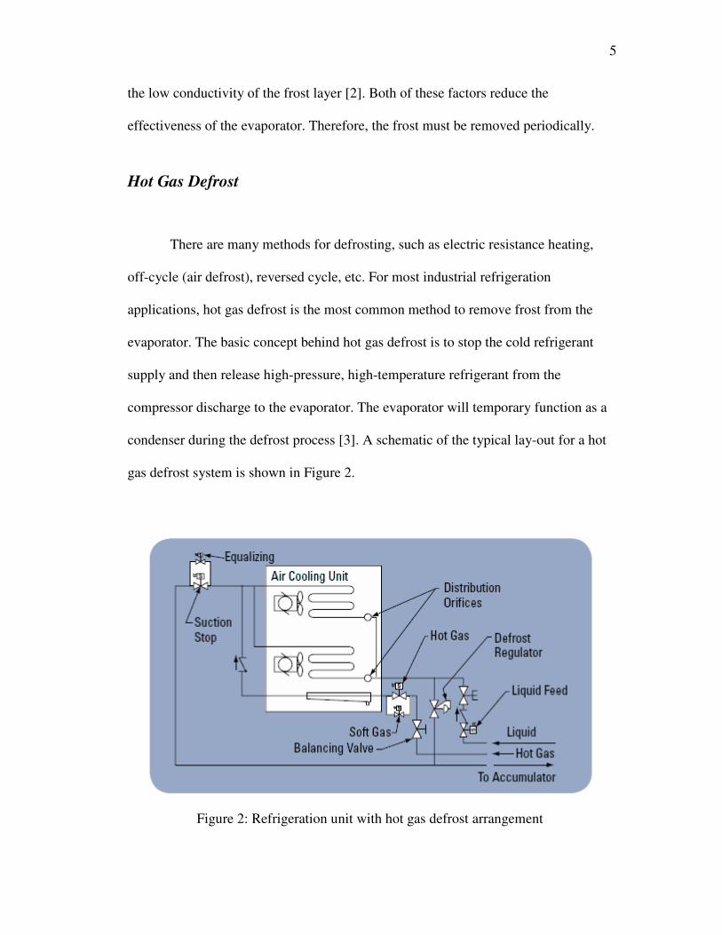
Hot Gas Defrost
There are many methods for defrosting, such as electric resistance heating,
off-cycle (air defrost), reversed cycle, etc. For most industrial refrigeration
applications, hot gas defrost is the most common method to remove frost from the
evaporator. The basic concept behind hot gas defrost is to stop the cold refrigerant
supply and then release high-pressure, high-temperature refrigerant from the
compressor discharge to the evaporator. The evaporator will temporary function as a
condenser during the defrost process [3]. A schematic of the typical lay-out for a hot
gas defrost system is shown in Figure 2.
Figure 2: Refrigeration unit with hot gas defrost arrangement
6
The processes of a typical hot gas defrost system are as follows:
Refrigeration (normal operation) phase:
• Saturated liquid refrigerant runs through the liquid feed valve into the evaporator
• Heat from the space is absorbed and the majority of the refrigerant is vaporized
• Saturated vapor from the evaporator outlet flows to the accumulator
Pump out phase (approximately 10 to 30 minutes):
• The liquid feed valve is closed
• The evaporator fans will continue to run in order for the liquid inside the coil to
vaporize which will prevent pressure shocks damage
• At the end of this phase, the fans are turned off and the suction stop valve will be
closed
Soft gas phase:
• For safety purposes, a solenoid valve is installed parallel to the hot gas valve to
allow the hot gas to flow slowly into the coil
• The main hot gas valve is opened while the solenoid valve is closed at the end of
this phase
7
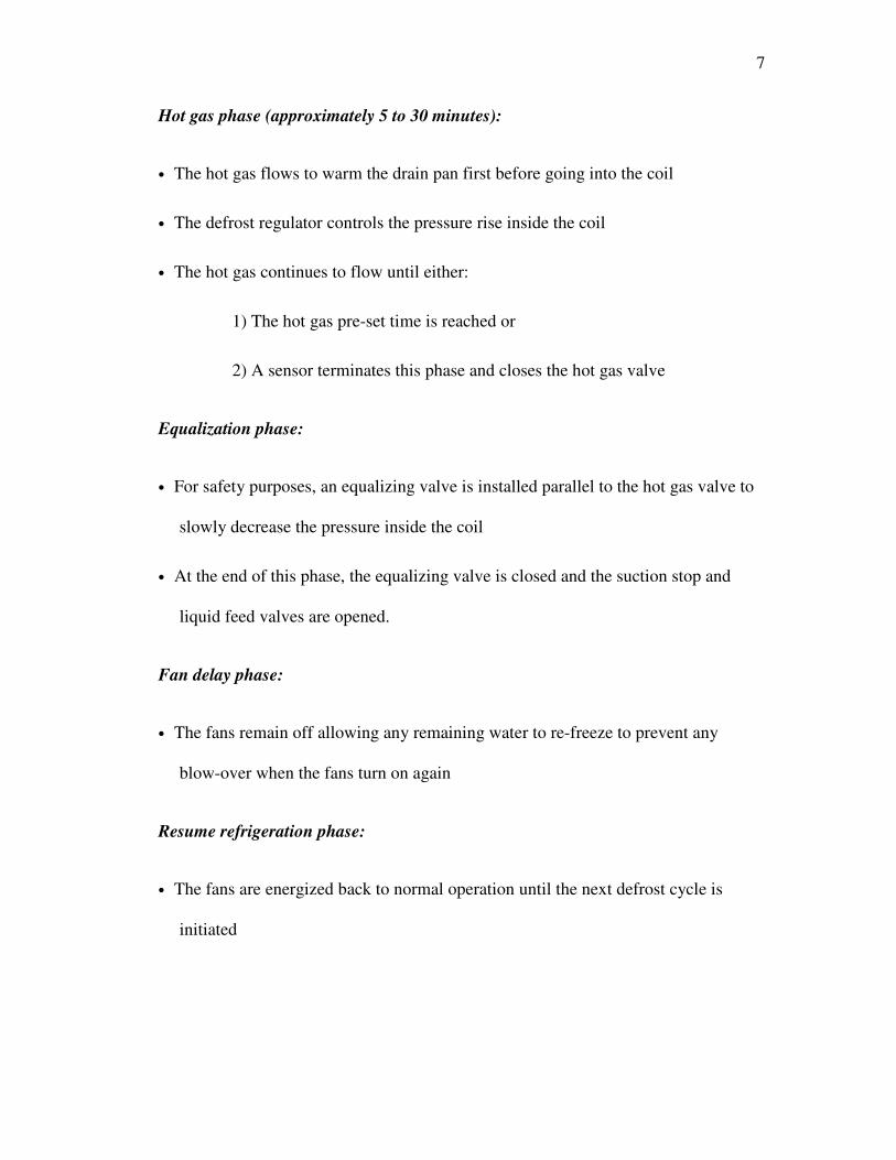
Hot gas phase (approximately 5 to 30 minutes):
• The hot gas flows to warm the drain pan first before going into the coil
• The defrost regulator controls the pressure rise inside the coil
• The hot gas continues to flow until either:
1) The hot gas pre-set time is reached or
2) A sensor terminates this phase and closes the hot gas valve
Equalization phase:
• For safety purposes, an equalizing valve is installed parallel to the hot gas valve to
slowly decrease the pressure inside the coil
• At the end of this phase, the equalizing valve is closed and the suction stop and
liquid feed valves are opened.
Fan delay phase:
• The fans remain off allowing any remaining water to re-freeze to prevent any
blow-over when the fans turn on again
Resume refrigeration phase:
• The fans are energized back to normal operation until the next defrost cycle is
initiated
8
Literature Review
There are two ways for frost to build up on the evaporator coil. The first type
is when tiny frost particles accumulate due to impaction on the evaporator coil
surfaces. The tiny frost particles are created from the supersaturated air stream that
suddenly cools. This type frost can build up very quickly due to its low density. It
forms when the moisture content in the air is high, for example, evaporative coils
near doors that open to the outside.
The second mechanism is through the diffusion of water vapor onto the cold
surface due to the difference in the concentration of water between the air stream and
the frost layer. This forms a layer of frost with high density. Due to the dense
structure, this type of frost must be removed periodically. This high density frost
occurs in places where the air temperature is low, along with low moisture content.
This type of frost forms on evaporator coils located inside a refrigerated warehouse
where food products are stored for a long period of time [1]. It is important to
periodically remove the frost on the coil surface regardless of the frost formation
mechanism, so that the evaporator can continue to operate normally.
There are many research studies for the prediction of frost growth.
Nevertheless, the frost formation is still an open research topic because there are
many different types of models, different assumptions and different experimental
conditions. Most of the frost prediction models can be categorized into three main
9
groups [4]. The first group uses molecular diffusion applied to the frost layer. Then,
empirical correlations on the air side are used to calculate heat and mass transfer to
predict the frost growth characteristics [5]. The second group applies an improved
model to predict the frost properties by using the empirical correlations from the air
flow boundary layer equations [6]. The third group uses molecular diffusion in the
frost layer combined with the boundary layer equations to analyze the frost
formation [7].
There are some studies that do not follow the previous mentioned groups.
Some of these studies focus on the analysis of simple geometries that resemble a
portion of a heat exchanger, such as a laminar flow analysis over parallel cold plates
[8], a frost formation study on a vertical plate [9], and an experimental analysis on a
cold cylindrical surface [10]. Some researchers have worked to develop realistic and
complex frost growth models. For example, Tso et al. created a more comprehensive
model by deriving equations for non-steady-state and quasi-steady state heat transfer
through a tube-fin heat exchanger [11]. Lenic et al. developed a transient two-
dimensional mathematical model of frost formation to predict the frost growth rate
and a change in the thermal conductivity of the frost layer [12].
Although there are many frost growth models, the majority of them do not
focus on when to initiate or terminate the hot gas defrost cycle. Hoffenbecker et al
developed a model of the hot gas defrost process [13]. For practical applications, this
10
method is easier to implement than other models and it still can produce reasonable
results, which is why Hoffenbecker’s model is chosen for this project.
Many models have been developed and experiments have been conducted to
study how to detect the frost build up and how the frost accumulation affects the
system performance. The pressure drop across the coil has been used numerous times
to predict frost growth, especially in heat pump applications. For example, Yao et al.
developed a distributed mathematical model of the airside heat exchanger under frost
conditions in an air source heat pump unit [14]. Liu et al. created a transient one
dimensional model to predict frost growth and validated it experimentally for a heat
pump unit [15]. Both researchers show that pressure drop increases dramatically
once the frost accumulates. As a result, pressure drop is investigated as a frost
detection method in this application as well.
Not many studies focus on cost estimation of the hot gas process. Cole is one
of the few researchers who has developed models to analyze the cost of the hot gas
defrost process [16].
11
Temperature Model
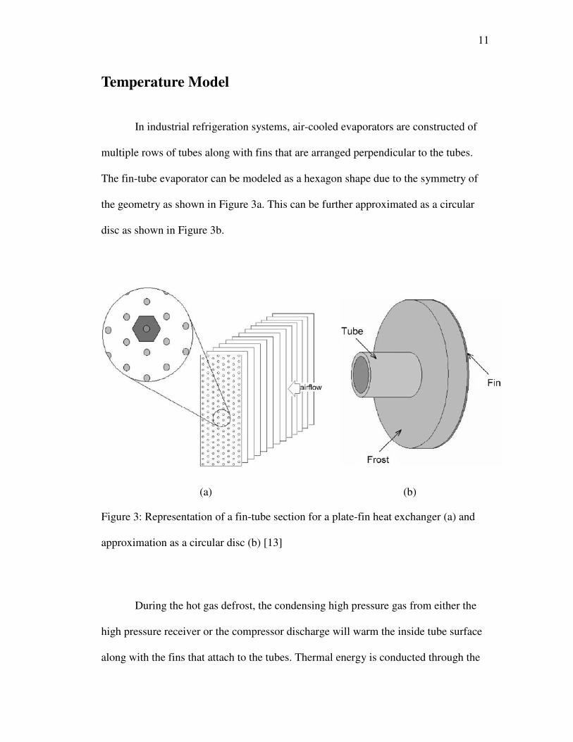
In industrial refrigeration systems, air-cooled evaporators are constructed of
multiple rows of tubes along with fins that are arranged perpendicular to the tubes.
The fin-tube evaporator can be modeled as a hexagon shape due to the symmetry of
the geometry as shown in Figure 3a. This can be further approximated as a circular
disc as shown in Figure 3b.
(a) (b)
Figure 3: Representation of a fin-tube section for a plate-fin heat exchanger (a) and
approximation as a circular disc (b) [13]
During the hot gas defrost, the condensing high pressure gas from either the
high pressure receiver or the compressor discharge will warm the inside tube surface
along with the fins that attach to the tubes. Thermal energy is conducted through the
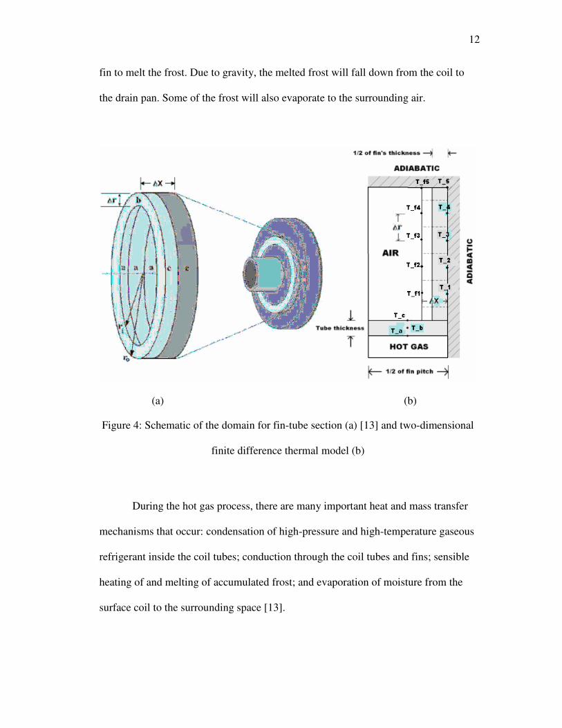
12
fin to melt the frost. Due to gravity, the melted frost will fall down from the coil to
the drain pan. Some of the frost will also evaporate to the surrounding air.
(a) (b)
Figure 4: Schematic of the domain for fin-tube section (a) [13] and two-dimensional
finite difference thermal model (b)
During the hot gas process, there are many important heat and mass transfer
mechanisms that occur: condensation of high-pressure and high-temperature gaseous
refrigerant inside the coil tubes; conduction through the coil tubes and fins; sensible
heating of and melting of accumulated frost; and evaporation of moisture from the
surface coil to the surrounding space [13].
13
A thermal model of the geometry shown in Figure 3 was developed to study
the hot gas defrost process. The fin-tube was modeled as a two-dimensional,
transient conduction problem. The heat equation for two-dimensional, axisymmetric
conduction is
.1
C
∂
∂
∂
∂+
∂
∂
∂
∂=
∂
∂
z
Tk
zr
Tkr
rrt
Tpρ (1)
The geometry is sub-divided into smaller regions, as shown in Figure 4, and the heat
transfer problem is solved using the finite difference method. The boundary
conditions for a control volume about each node are:
• Boundary a: thermal conduction from the adjoining nodes at the inner radius.
• Boundary b: conduction/convection in the axial direction at the left side
• Boundary c: thermal conduction to the adjoining nodes at the outer radius
• Boundary d: thermal conduction in the axial direction at the right side
An adiabatic boundary condition is applied at the outer radius and the right side of
the model as shown in Figure 4b. The boundary condition at the inside tube wall is
assumed to be constant temperature due to the condensing refrigerant. The boundary
condition on the left side is convective heat and mass transfer to the surrounding air.
14
The two dimensional axisymmetric, partial differential equation is solved using a
finite difference approach. The difference equation for node T_1 is
(2)
The first term on the left hand side of equation (2) represents the change in
energy stored in the node. This can be simplified by changing dh = CpdT and
assuming that Cp is constant. The first and second terms on the right hand side of
equation (2) represent thermal conduction in the radial direction. The third term on
the right hand side represents the thermal conduction between adjacent nodes from
the fin to the frost at the same radial location. The energy balance at different radial
locations along the fin will have a similar set up.
( )( )
( )( )
( )( )
( ) .222
2
/In22
/In22
1frost1
2
1
2
12
12
21
1
1
−
+
+
+−
+
−−∆
−−∆
=
TTtktk
kkrrrr
rr
TTxk
rr
TTxk
dt
dhV
frostfinfinfrost
frostfinc
fin
c
c
fin
π
ππρ
15
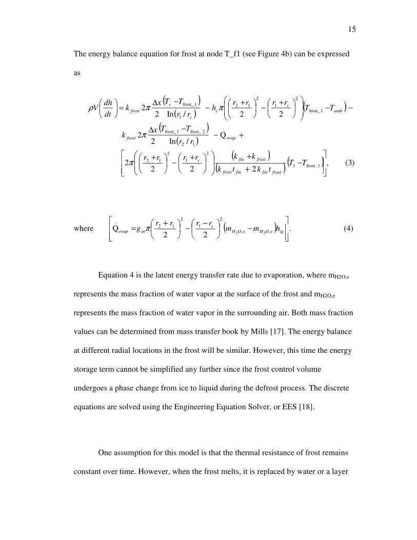
The energy balance equation for frost at node T_f1 (see Figure 4b) can be expressed
as
where ( ) .22
Q ,,
2
1
2
12.
22
−
−−
+= igeOHsOH
c
mevap hmmrrrr
g π (4)
Equation 4 is the latent energy transfer rate due to evaporation, where mH2O,s
represents the mass fraction of water vapor at the surface of the frost and mH2O,e
represents the mass fraction of water vapor in the surrounding air. Both mass fraction
values can be determined from mass transfer book by Mills [17]. The energy balance
at different radial locations in the frost will be similar. However, this time the energy
storage term cannot be simplified any further since the frost control volume
undergoes a phase change from ice to liquid during the defrost process. The discrete
equations are solved using the Engineering Equation Solver, or EES [18].
One assumption for this model is that the thermal resistance of frost remains
constant over time. However, when the frost melts, it is replaced by water or a layer
( )( )
( )
( )( )
( )( )
( ) )3(,222
2
Q/In2
2
22/In22
1frost_1
2
1
2
12
.
12
2frost_1frost_
1frost_
2
1
2
12
1
1frost_
−
+
+
+−
+
+−−∆
−−
+−
+−
−∆=
TTtktk
kkrrrr
rr
TTxk
TTrrrr
hrr
TTxk
dt
dhV
frostfinfinfrost
frostfinc
evapfrost
amb
c
c
c
c
frost
π
π
ππρ
16
of air, which cause a change in the thermal resistance. It is difficult to model the
change in thermal resistance under these conditions because of the uncertainty in
determining the substance/phase within the layer as a function of time. This approach
was taken in order to develop a reasonably accurate yet somewhat simple model.
17
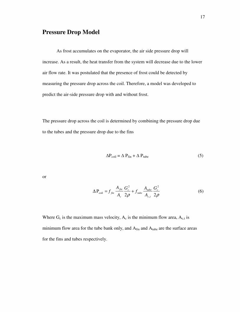
Pressure Drop Model
As frost accumulates on the evaporator, the air side pressure drop will
increase. As a result, the heat transfer from the system will decrease due to the lower
air flow rate. It was postulated that the presence of frost could be detected by
measuring the pressure drop across the coil. Therefore, a model was developed to
predict the air-side pressure drop with and without frost.
The pressure drop across the coil is determined by combining the pressure drop due
to the tubes and the pressure drop due to the fins
∆Pcoil = ∆ Pfin + ∆ Ptube (5)
or
ρρ 22
P2
,
2
coilc
tc
tube
tube
c
c
fin
fin
G
A
Af
G
A
Af +=∆ (6)
Where Gc is the maximum mass velocity, Ac is the minimum flow area, Ac,t is
minimum flow area for the tube bank only, and Afin and Atube are the surface areas
for the fins and tubes respectively.
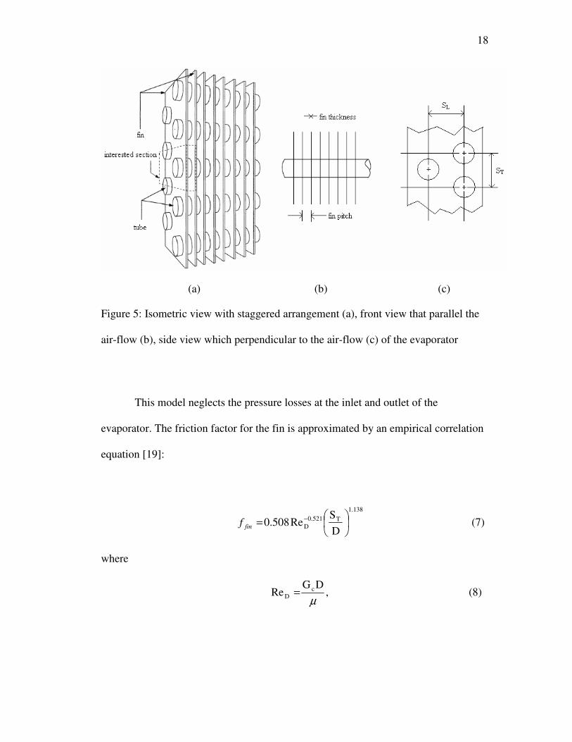
18
(a) (b) (c)
Figure 5: Isometric view with staggered arrangement (a), front view that parallel the
air-flow (b), side view which perpendicular to the air-flow (c) of the evaporator
This model neglects the pressure losses at the inlet and outlet of the
evaporator. The friction factor for the fin is approximated by an empirical correlation
equation [19]:
138.1
T521.0
DD
SRe508.0
= −
finf (7)
where
,DG
Re cD
µ= (8)
19
ST is defined as the transverse pitch or tube spacing normal to the air flow (shown in
Figure 5c), and µ is defined as the viscosity of air. The Reynolds number is based on
the tube outer diameter and the maximum fluid velocity occurring within the tube
bank. The maximum velocity is defined as
( )( )( )
.max VthicknessfinpitchfinDS
thicknessfinpitchfinSV
tubeT
T
−−
−= (9)
Some researchers use the friction factor for the tube based on the Zukauskas
correlation for both normal and staggered banks of tubes. For this pressure drop
model, the friction factor for the tube can be approximate from Figure 6 [20],
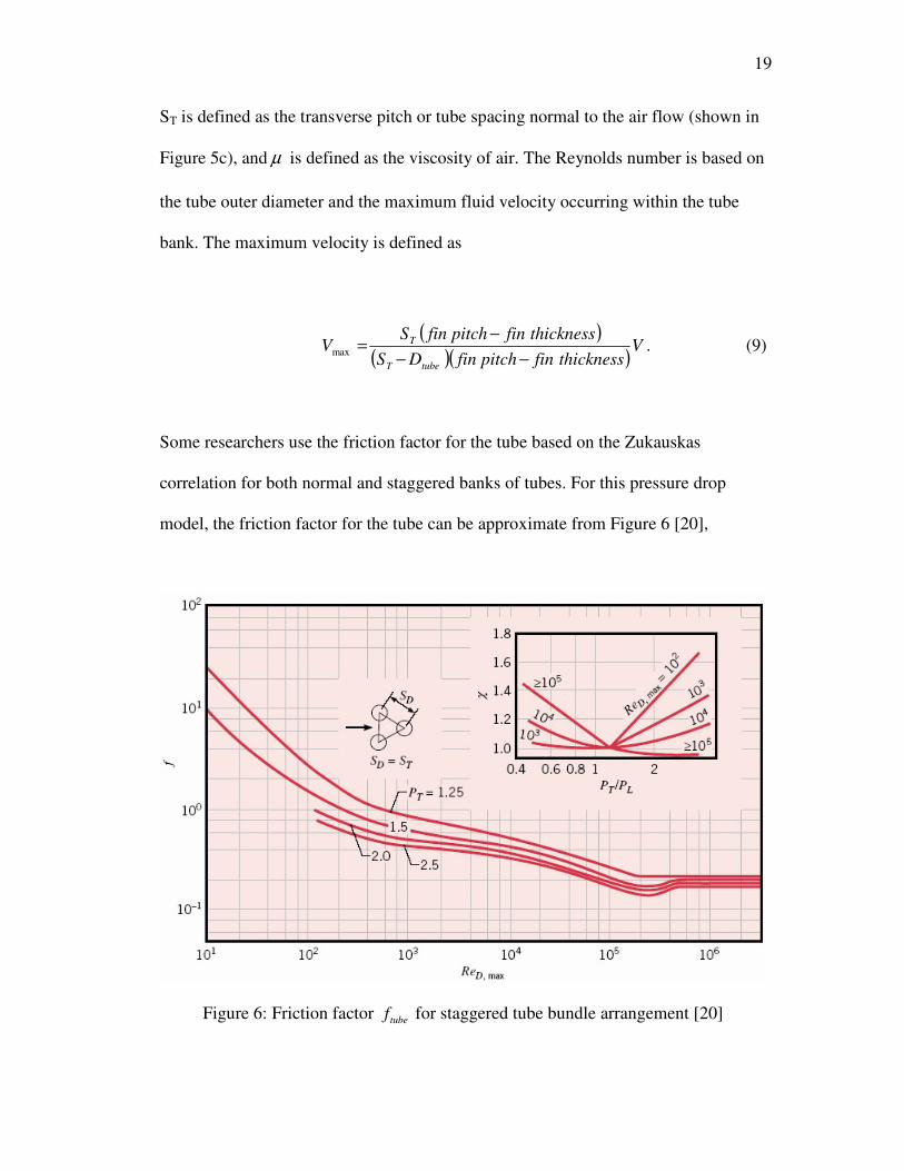
Figure 6: Friction factor tubef for staggered tube bundle arrangement [20]
20
where PT is defined as ST/D which is the dimensionless transverse pitch.
The pressure drop for the coil with frost is modeled by assuming that the frost layer
simply increases the fin thickness and the tube outer diameter. The frost layer is
assumed to have uniform thickness and the increased roughness of the frost layer is
neglected.
21
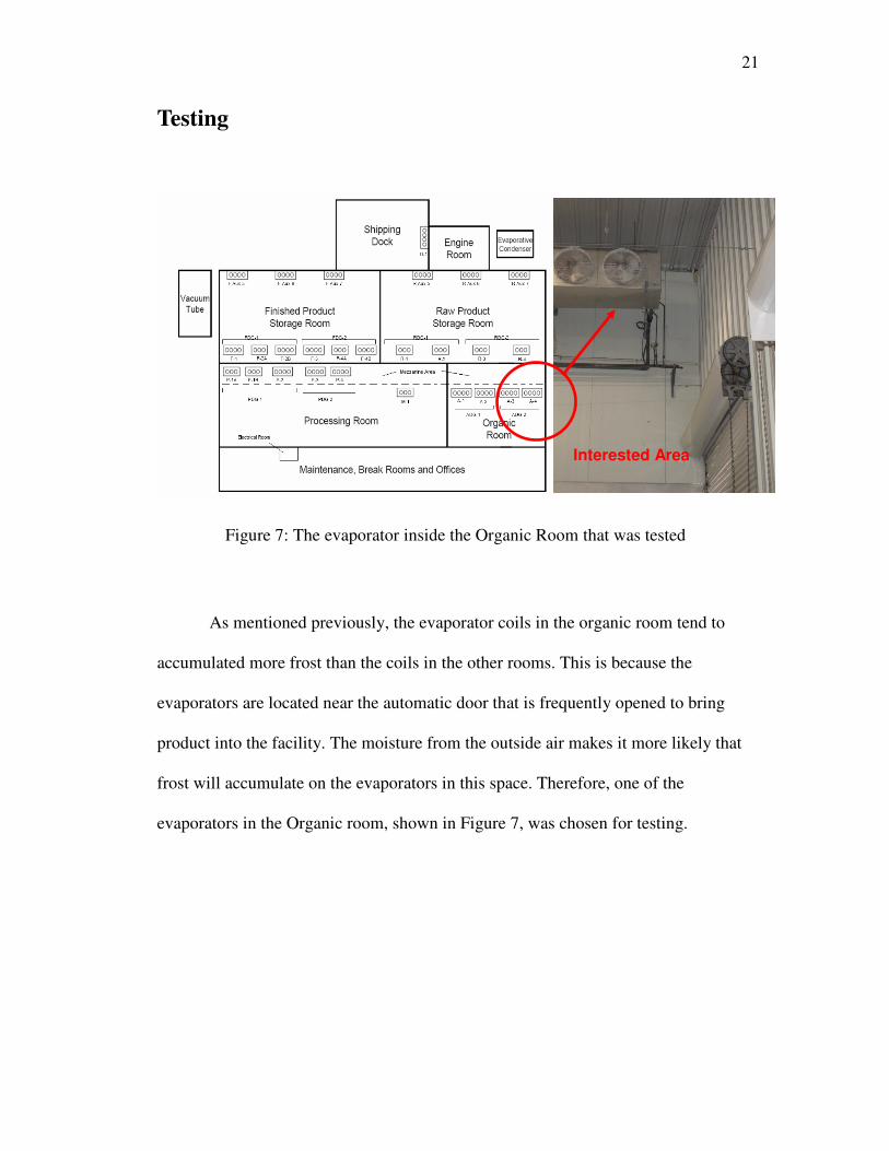
Testing
Figure 7: The evaporator inside the Organic Room that was tested
As mentioned previously, the evaporator coils in the organic room tend to
accumulated more frost than the coils in the other rooms. This is because the
evaporators are located near the automatic door that is frequently opened to bring
product into the facility. The moisture from the outside air makes it more likely that
frost will accumulate on the evaporators in this space. Therefore, one of the
evaporators in the Organic room, shown in Figure 7, was chosen for testing.
Interested Area
22
Collecting Data
Opto system
The Opto22 system is used as the main control system for the Classic Salads
facility [21]. The following is the list of sensors connected to the Opto22 system:
• Zone temperature - air temperature measured at the inlet of the coil
• Zone suction temperature – refrigerant temperature measured at the outlet of the
coil
• AU VFD SR – fan speed
• Zone coil temperature – temperature measured at the tube sheet on evaporator
• Discharge pressure – main system discharge pressure at the outlet of the condenser
Two wire RTD are used to measure temperature for the Opto22 system.
HOBO System
The coil was instrumented with additional sensors and the output from these
sensors was recorded with a HOBO U12-006 model data logger, which is shown in
Figure 8. The HOBO data logger has 4 channels and can record up to 43,000
measurements [22]. The coil was instrumented with 3 temperature sensors and 1
pressure transducer. Data was logged from November 9, 2008 at 8 am to November
15, 2008 at 7 pm. The temperature sensors were two wire RTD. Each RTD utilized a
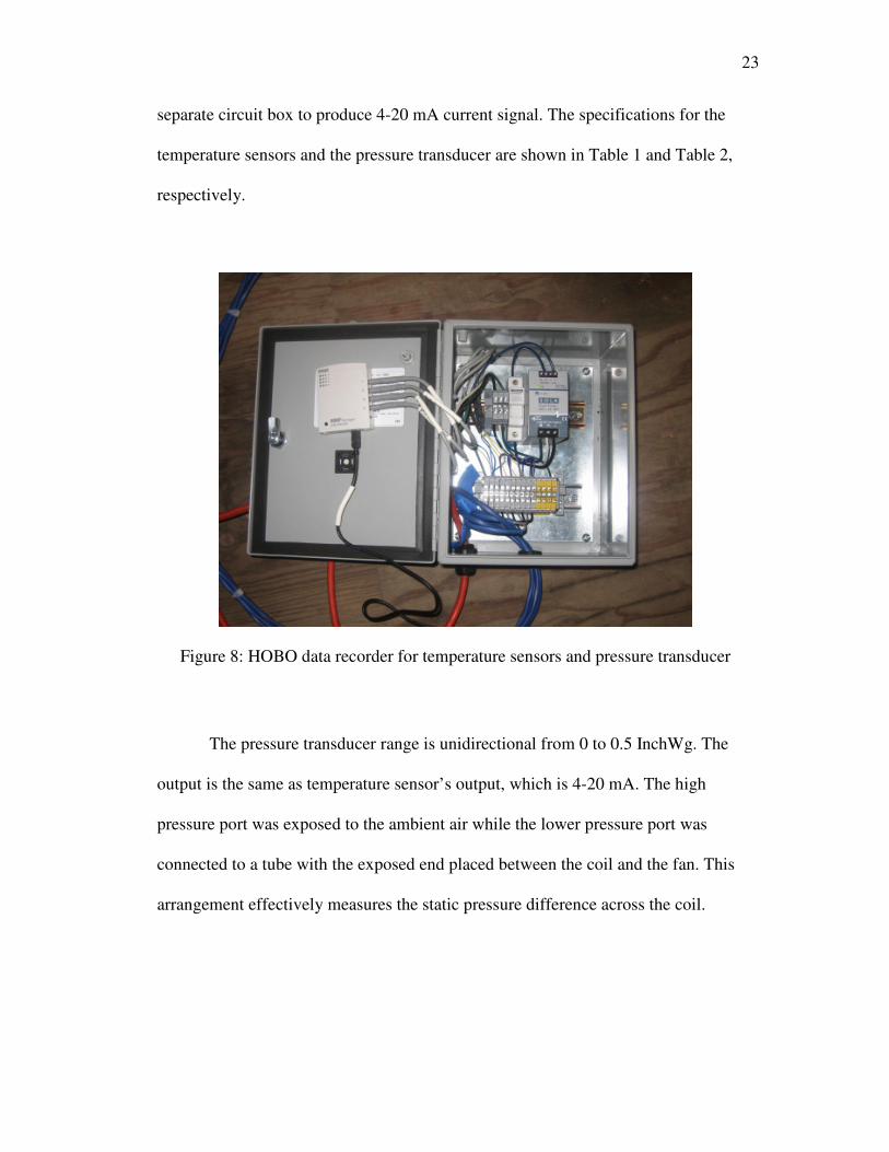
23
separate circuit box to produce 4-20 mA current signal. The specifications for the
temperature sensors and the pressure transducer are shown in Table 1 and Table 2,
respectively.
Figure 8: HOBO data recorder for temperature sensors and pressure transducer
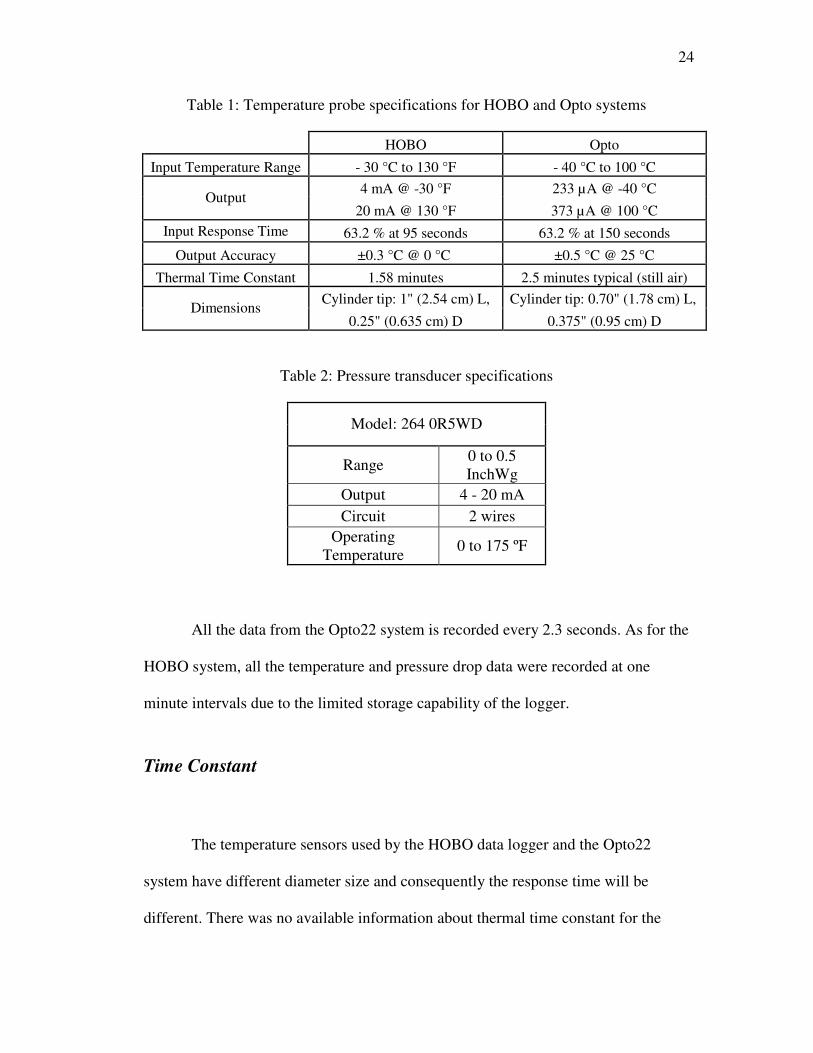
The pressure transducer range is unidirectional from 0 to 0.5 InchWg. The
output is the same as temperature sensor’s output, which is 4-20 mA. The high
pressure port was exposed to the ambient air while the lower pressure port was
connected to a tube with the exposed end placed between the coil and the fan. This
arrangement effectively measures the static pressure difference across the coil.
24
Table 1: Temperature probe specifications for HOBO and Opto systems
HOBO Opto
Input Temperature Range - 30 °C to 130 °F - 40 °C to 100 °C
4 mA @ -30 °F 233 µA @ -40 °C Output
20 mA @ 130 °F 373 µA @ 100 °C
Input Response Time 63.2 % at 95 seconds 63.2 % at 150 seconds
Output Accuracy ±0.3 °C @ 0 °C ±0.5 °C @ 25 °C
Thermal Time Constant 1.58 minutes 2.5 minutes typical (still air)
Cylinder tip: 1" (2.54 cm) L, Cylinder tip: 0.70" (1.78 cm) L, Dimensions
0.25" (0.635 cm) D 0.375" (0.95 cm) D
Table 2: Pressure transducer specifications
Model: 264 0R5WD
Range 0 to 0.5 InchWg
Output 4 - 20 mA
Circuit 2 wires
Operating Temperature
0 to 175 ºF
All the data from the Opto22 system is recorded every 2.3 seconds. As for the
HOBO system, all the temperature and pressure drop data were recorded at one
minute intervals due to the limited storage capability of the logger.
Time Constant
The temperature sensors used by the HOBO data logger and the Opto22
system have different diameter size and consequently the response time will be
different. There was no available information about thermal time constant for the
25
RTD used by the HOBO data logger. Therefore, an experiment was conducted to
determine the response time.
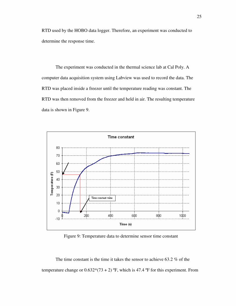
The experiment was conducted in the thermal science lab at Cal Poly. A
computer data acquisition system using Labview was used to record the data. The
RTD was placed inside a freezer until the temperature reading was constant. The
RTD was then removed from the freezer and held in air. The resulting temperature
data is shown in Figure 9.
Figure 9: Temperature data to determine sensor time constant
The time constant is the time it takes the sensor to achieve 63.2 % of the
temperature change or 0.632*(73 + 2) ºF, which is 47.4 ºF for this experiment. From
26
Figure 9, the time constant is determined to be approximately 95 seconds. The first
53 seconds is when the RTD is still inside the refrigerator at a temperature of
approximately -2 ºF. After that, the RTD is taken out from the refrigerator to the
ambient air, which is at approximately 73 ºF. The time to reach steady state is
approximately 600 seconds. This is approximately 37% faster than the response time
of the temperature sensor used by the Opto22 system (see Table 1).
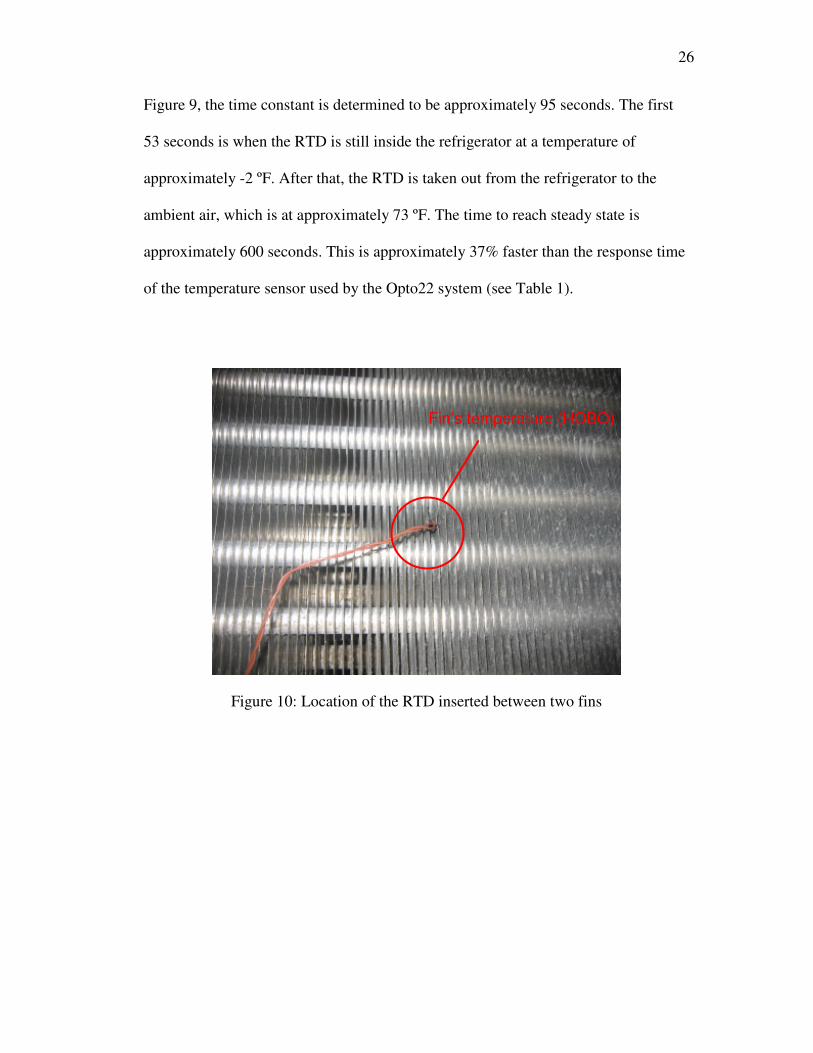
Figure 10: Location of the RTD inserted between two fins
Fin’s temperature (HOBO)
27
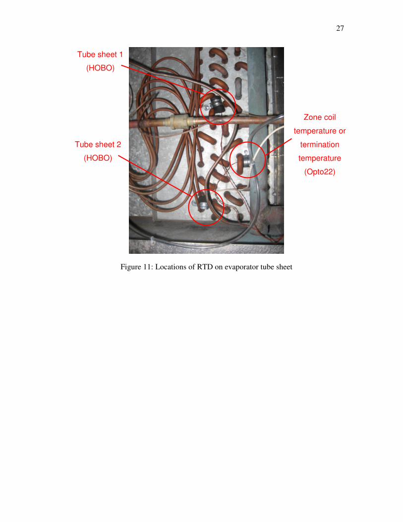
Figure 11: Locations of RTD on evaporator tube sheet
Zone coil
temperature or
termination
temperature
(Opto22)
Tube sheet 2
(HOBO)
Tube sheet 1
(HOBO)
28
Results
Temperature
8 am to 2 pm (11/09/08)
30
35
40
45
50
55
120 125 130 135 140 145 150 155 160 165 170
Time (min)
Tem
mp
era
ture
(F
)
Fin temp
Tube sheet temp 1
Tube sheet temp 2
Inlet air T
Outlet T
Termination T
Figure 12: Temperature data from Opto22 and HOBO systems during the defrost
cycle
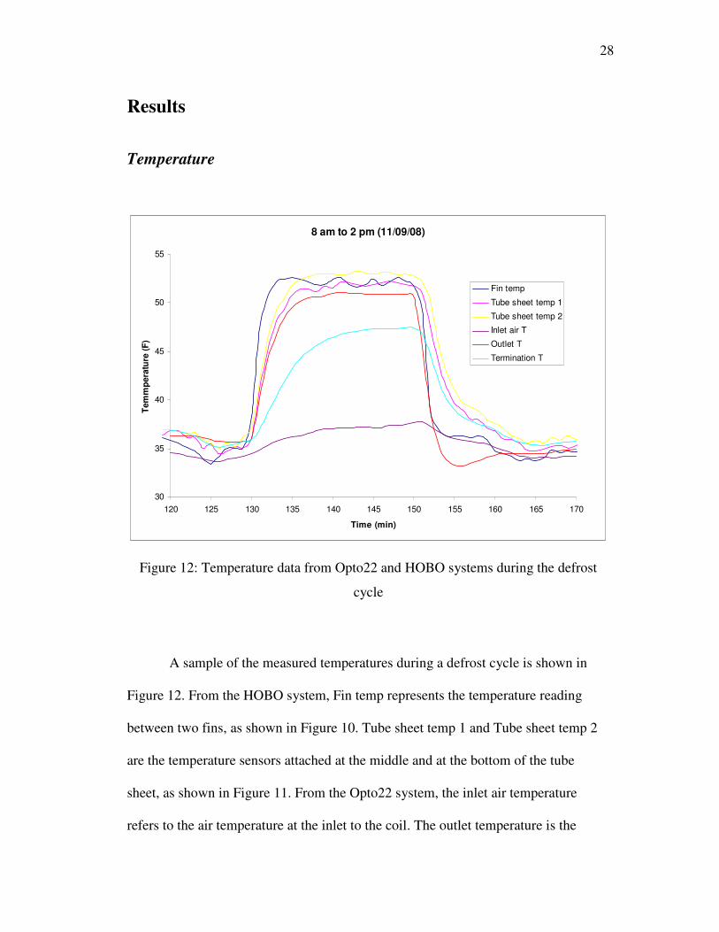
A sample of the measured temperatures during a defrost cycle is shown in
Figure 12. From the HOBO system, Fin temp represents the temperature reading
between two fins, as shown in Figure 10. Tube sheet temp 1 and Tube sheet temp 2
are the temperature sensors attached at the middle and at the bottom of the tube
sheet, as shown in Figure 11. From the Opto22 system, the inlet air temperature
refers to the air temperature at the inlet to the coil. The outlet temperature is the
29
sensor attached to the suction line of the coil. The termination temperature is
attached on the tube sheet which is shown in Figure 11.
Note that none of the temperature readings are below 32 ºF which indicates
that there might not be much frost accumulated. This result is representative for data
collected during the entire week. The temperature readings from the tube sheet seem
to be more stable in comparison to the reading for the sensor between the fins. This
may be due to the insulation that covering around the temperature sensors on the
tube sheet, while the temperature sensor attached between the fins is exposed to the
surrounding air.
The termination temperature sensor (Opto22 system) attached to the tube
sheet responded slowly compared to the HOBO temperature sensors that were also
attached to the tube sheet. The Opto22 sensor took more than 10 minutes to reach
steady state while it took about 5 minutes for the HOBO sensors. Also, the Opto22
temperature measurement is approximately 5 degrees lower in comparison to the
measurements made by the HOBO sensors. The reason for these different values is
unknown.
The temperature sensor attached between the fins appeared to have a quick
response time compared to the other sensors. This indicates that temperature sensor
between the fins should yield a more accurate representation of the temperature of
30
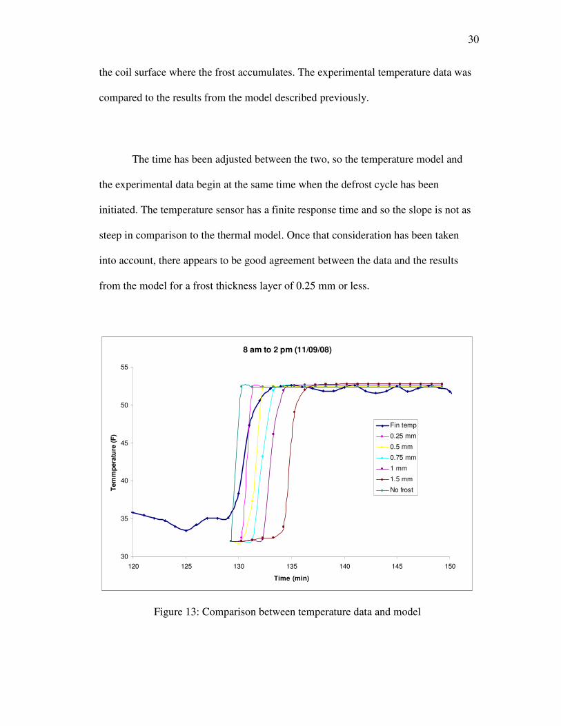
the coil surface where the frost accumulates. The experimental temperature data was
compared to the results from the model described previously.
The time has been adjusted between the two, so the temperature model and
the experimental data begin at the same time when the defrost cycle has been
initiated. The temperature sensor has a finite response time and so the slope is not as
steep in comparison to the thermal model. Once that consideration has been taken
into account, there appears to be good agreement between the data and the results
from the model for a frost thickness layer of 0.25 mm or less.
8 am to 2 pm (11/09/08)
30
35
40
45
50
55
120 125 130 135 140 145 150
Time (min)
Tem
mp
era
ture
(F
)
Fin temp
0.25 mm
0.5 mm
0.75 mm
1 mm
1.5 mm
No frost
Figure 13: Comparison between temperature data and model
31
Figure 13 shows measured data for the temperature of the fin (Fin temp),
along with results from the finite difference model for frost layers with different
thicknesses. The result for node 5 of the model (midway between tubes, see Figure
4b) was used for the comparison. For all the nodes, the initial temperature starts at
the freezing point of water but experimentally none of the fin’s temperature readings
reached 32 ºF. This was done so the accumulation of frost could be modeled.
Figure 14: Fin temperature during hot gas defrost with 1 mm of frost
32
Figure 15: Fin temperature during hot gas defrost with 0.5 mm of frost
Figures 14 and 15 show the results of the nodal temperatures during a defrost
simulation. The initial temperature for all nodes is 32 F. Figure 14 is for a frost layer
of 1 mm and Figure 15 is for a frost layer of 0.5 mm. The subscript for each
temperature is defined in Figure 4b with the inner radius being 1 and the other radius
being 5. It takes approximately 250 seconds the temperatures to reach steady state
with 0.5 mm of frost, while it takes about 400 seconds for the temperature to reach
steady state with 1 mm of frost.
33
Figure 16: Heat transfer during hot gas defrost with 0.5 mm of frost
Figure 17: Heat transfer during hot gas defrost with 1 mm of frost
34
Figures 16 and 17 show the resulting heat rates during a defrost simulation.
Qin, total is defined as the total heat going into system from the hot gas. Qconv, total is the
heat lost due to convection and Qmelt is the heat required to melt the frost. The
figures show the total energy integrated over time. The time to melt the frost can be
observed from the figures by noting when Qmelt becomes constant. After this point,
heat from the hot gas is lost due to convection.
Pressure drop
2 pm to 8 pm (11/10/08)
0.25
0.3
0.35
0.4
0.45
0.5
0 20 40 60 80 100 120
Time (min)
Pre
ssu
re D
rop
(In
ch
Wg
)
P drop
Mean value
Mean + STD V
Mean - STD V
Figure 18: Sample of coil pressure drop data
35
Figure 18 shows the measured pressure drop as a function of time during
normal operation. The mean value, of the pressure for the period shown in Figure 18
is 0.403 InchWg. The standard deviation of the readings is 0.019 InchWg. The data
is a representative of the data collected for the entire week.
There is significant scatter in the data, which may indicate the pressure tap
was not rigidly fixed. Regardless, there is no general trend of increasing pressure
drop with time, which would indicate the buildup of frost on the coil.
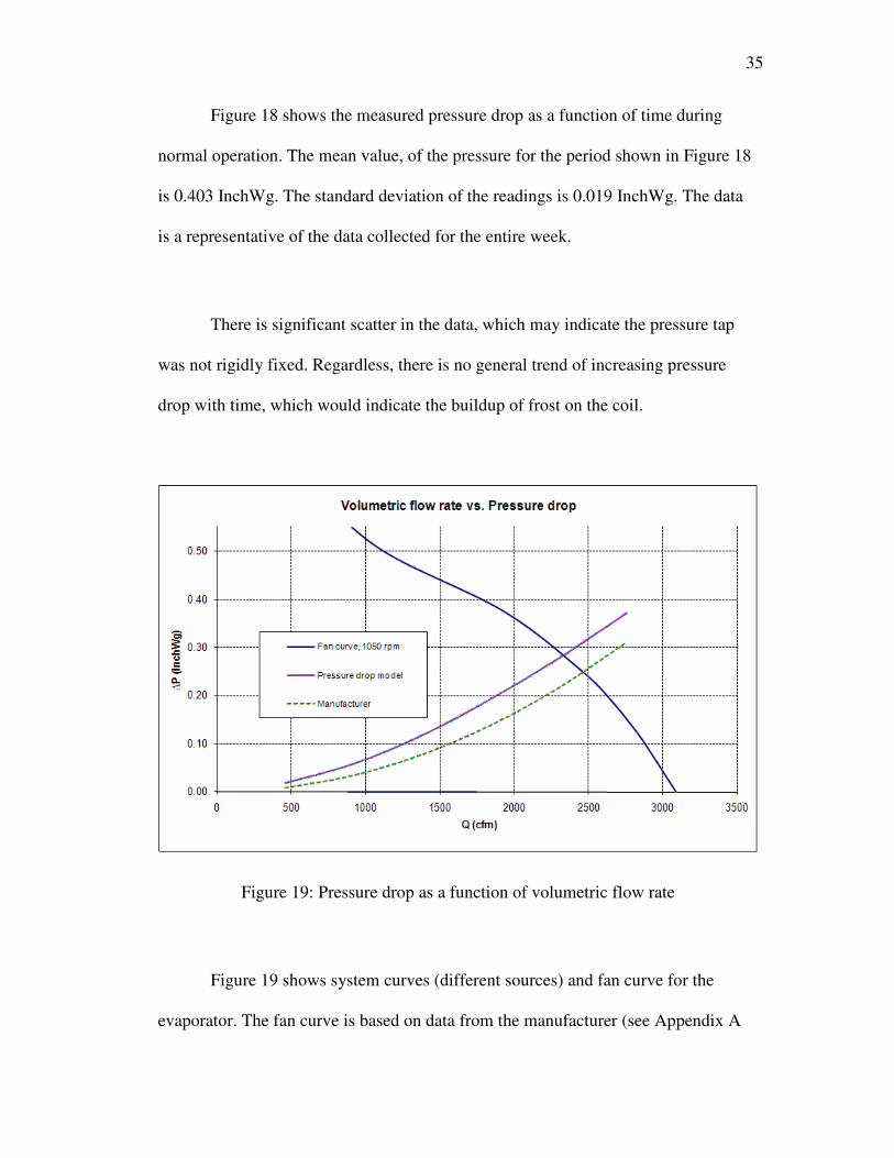
Figure 19: Pressure drop as a function of volumetric flow rate
Figure 19 shows system curves (different sources) and fan curve for the
evaporator. The fan curve is based on data from the manufacturer (see Appendix A
36
for more information). The “manufacturer” system curve is extrapolated from a
single data point assuming 2QαP∆ . The pressure drop as determined by the model is
also shown over the range of flow rates.
Figure 19 shows reasonably good agreement between the manufacturer’s data
and the pressure drop model. The measured pressure drop exceeds the pressure drop
from the manufacturer’s data and the model. This may be due to foreign particles,
such as cardboard fibers, which have buildup on the coil surface.
Volumetric flow rate vs. Pressure drop
0.00
0.10
0.20
0.30
0.40
0.50
0.60
0.70
0.80
0.90
0 500 1000 1500 2000 2500 3000 3500
Q (cfm)
∆P
(In
ch
Wg
)
1050 rpm
without frost
0.25 mm of frost
0.5 mm of frost
0.75 mm of frost
1 mm of frost
Figure 20: Pressure drop as a function of volumetric flow rate for different frost
thicknesses
37
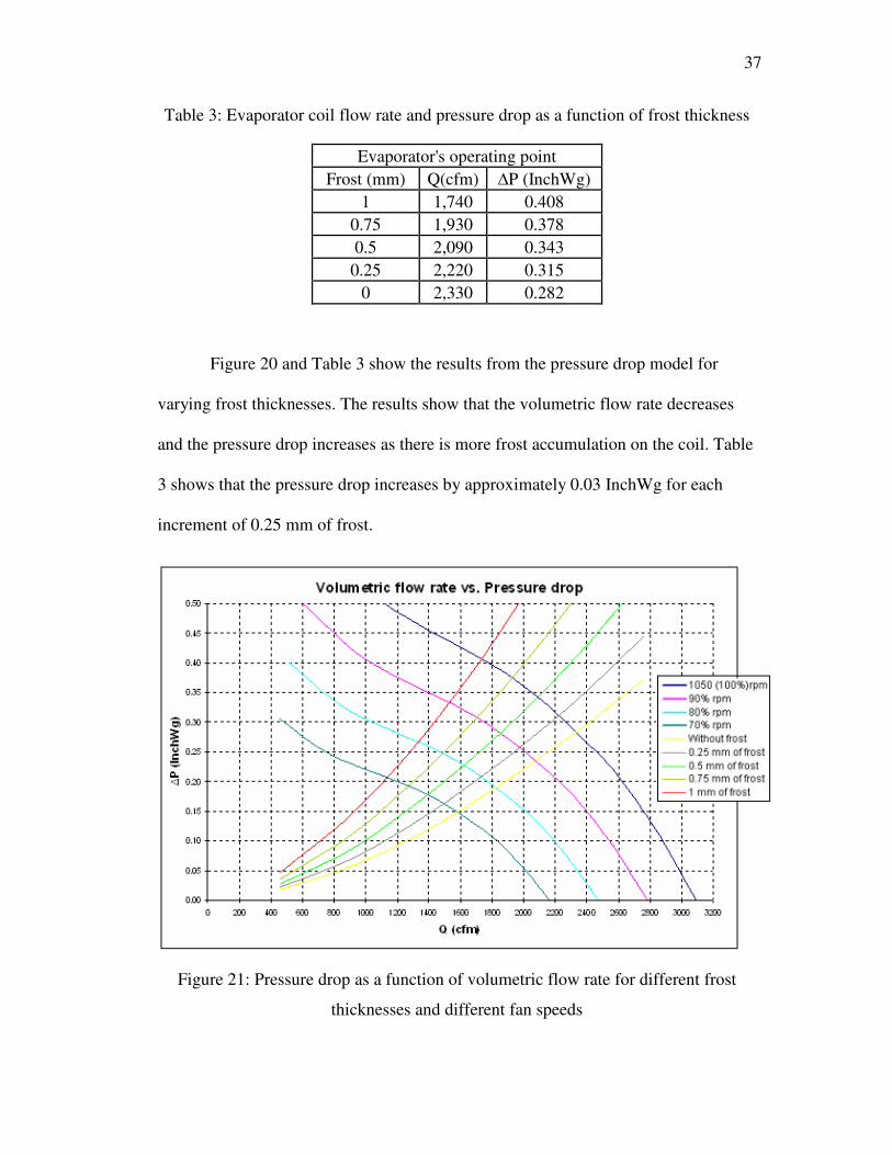
Table 3: Evaporator coil flow rate and pressure drop as a function of frost thickness
Evaporator's operating point
Frost (mm) Q(cfm) ∆P (InchWg)
1 1,740 0.408
0.75 1,930 0.378
0.5 2,090 0.343
0.25 2,220 0.315
0 2,330 0.282
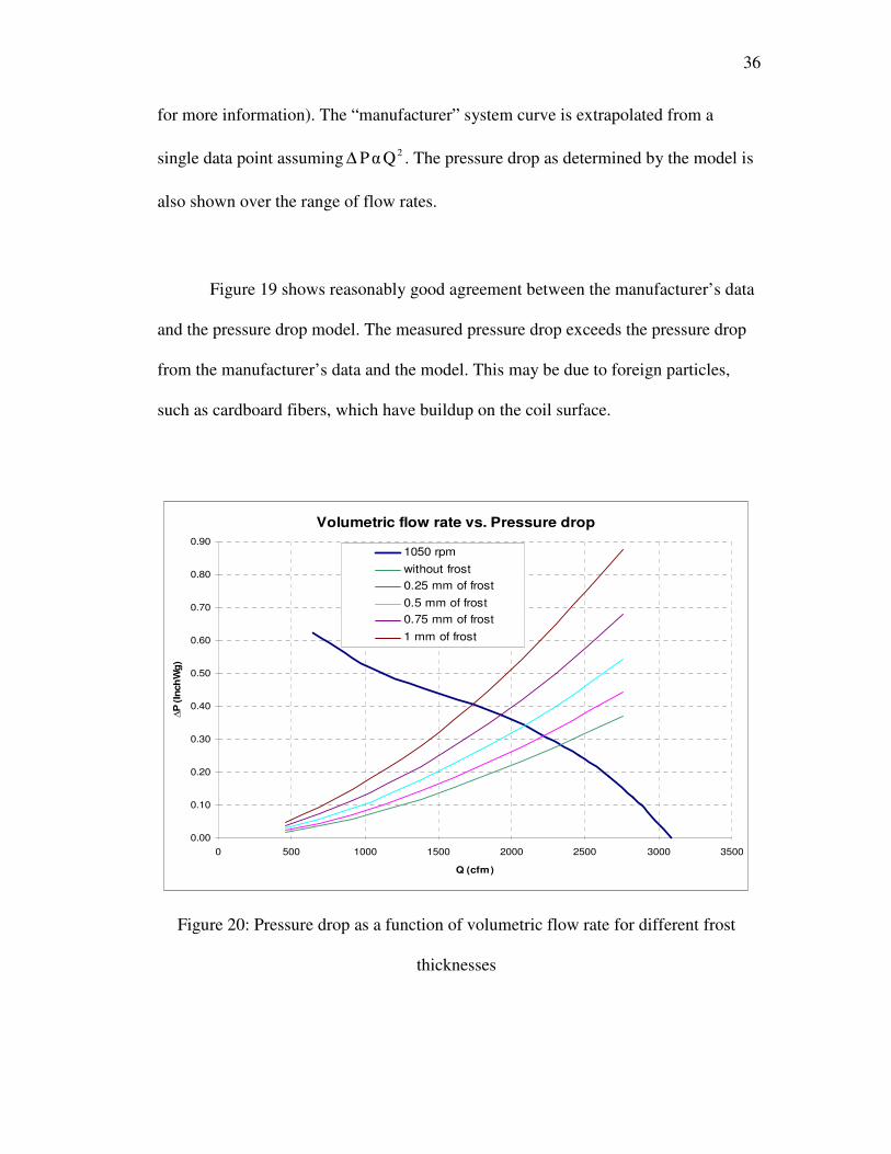
Figure 20 and Table 3 show the results from the pressure drop model for
varying frost thicknesses. The results show that the volumetric flow rate decreases
and the pressure drop increases as there is more frost accumulation on the coil. Table
3 shows that the pressure drop increases by approximately 0.03 InchWg for each
increment of 0.25 mm of frost.
Figure 21: Pressure drop as a function of volumetric flow rate for different frost
thicknesses and different fan speeds
38
Figure 21 shows the same set of system curves from Figure 20 along with a
set of fan curves at speeds varying from 70% to 100% of full speed (1050 rpm) .The
pressure drop will increase from 0.282 InchWg (dry coil) to 0.408 InchWg with 1
mm of frost when the system is operated at 100% fan speed. If the system operates at
70% of the fan speed (735 rpm), then the pressure drop will increase from 0.147
InchWg (dry coil) to 0.205 InchWg with 1 mm of frost. This shows that as the fan
speed decreases the difference in the pressure drop will also decrease. Therefore, it
will be harder to detect the amount of frost on the coil using a pressure sensor when
the system operates at lower fan speed.
Efficiency and Cost
The defrost efficiency is defined as
total
meltdefrost
Q
Q=η (10)
Where Qmelt is total heat required to warm and melt the frost on the coil and
Qtotal is the total heat transfer to the coil during the defrost. A defrost efficiency
closer to 1 indicates that a majority of the heat is used to melt the frost.
39
Eff vs. time for different h @ 1 mm
0.0
0.1
0.2
0.3
0.4
0.5
0.6
0.7
0.8
0.9
1.0
1 3 5 7 9 11 13 15 17 19Time (min)
Eff
h = 2
h = 5
h = 10
h = 15
h = 20
h = 25
Figure 22: Hot gas defrost efficiency as a function of defrost time for different
frost thickness
Figure 22 shows the defrost efficiency as a function of time for varying frost
thicknesses. The results were obtained from the thermal model. Figure 22 shows that
the efficiency of the hot gas defrost decreases with increasing time. Also, the
efficiency of the defrost decreases as the frost thickness decreases. These results
make sense because initially most of the energy is used to melt the frost. After that,
heat is transferred to the space by convection. A thinner frost layer will defrost more
rapidly and the defrost efficiency will be lower for a fixed defrost time. As
mentioned previously, the thermal resistance of the frost layer was not reduced as the
frost melted. Therefore, the efficiency of the real system will be lower than what is
shown in Figure 22.

40
The work input for a defrost system is defined as
βn
cycle
QW i= , (11)
where Qin is the excess heat generated from the hot gas after the frost has
melted and β is the coefficient of performance of the refrigeration system. Qin can
be expressed as: Qtotal – Qmelt. After substituting Qmelt = defrostη Qtotal from equation 11,
the work input can now be expressed as
( )β
ηdefrosttotalcycle
1QW
−= . (12)
Therefore, the cost for a defrost cycle is defined as:
Cost = ( )
−
β
ηdefrosttotal 1Q
kWh
$. (13)
For sample calculation, the coefficient of performance is assumed to be 3 and the
electricity cost is assumed to be $ 0.12 per kWh, based on 2009 Energy Information
Administration data [23].
41
Cost vs. defrost time
$0.00
$0.01
$0.02
$0.03
$0.04
$0.05
$0.06
$0.07
$0.08
$0.09
$0.10
0 2 4 6 8 10 12 14 16 18 20
Time (min)
Co
st
($)
0.25 mm
0.5 mm
0.75 mm
1 mm
1.5 mm
Figure 23: Hot gas defrost cost as a function of defrost time for different frost
thickness
Figure 23 shows the cost of operation will consequently increase as the
longer the system has to defrost. For thicker frost layers, all the energy from the hot
gas is used to melt the frost and so the cost is low initially. Thinner frost layers are
melted very quickly and the remaining heat goes to heat up the space instead. For 1
mm of frost, it costs about $ 0.08 for 20 minutes of defrost. If the system is
terminated 10 minutes sooner, it will cost only $ 0.035, which will save $ 0.045 per
defrost cycle.
42
Conclusions & Recommendations
Both the results from the measurements and the modeling indicate that there
was no frost build up during the testing at the Classic Salads facility. Although there
was scatter in the pressure measurements, there was no overall increase in the
pressure measurement with time, which would indicate the presence of frost on the
coil. The finite difference model with little or no frost was in good agreement with
the measured temperatures during a defrost cycle.
The Opto 22 temperature measurement on the tube sheet was significantly
different than the HOBO measurements on the fin and the tube sheet. First, the
Opto22 sensor had a longer lag time. Second, at steady state, there was about a 5°F
temperature difference between the measurements using the two systems. It may be
possible to use a temperature measurement to terminate the defrost cycle. A sensor
located on the fins should give a more accurate measure of the temperature of the
coil surface and whether frost is present. However, the lag in the Opto22 sensor (due
to the larger size) would make this measurement more conservative.
There was significant scatter in the pressure measurements, much larger than
the accuracy of the transducer. It is believed that the exposed end of the tube
between the fan and the coil was not properly attached and consequently was moving
due to the turbulence within the air stream. Also, the measured pressure drop across
43
the coil was higher than that measured by the manufacturer and predicted by the
model. The reason for this could be due to cardboard fiber accumulation on the
surfaces of the coil.
The purpose of the pressure measurement was to determine whether the
defrost cycle could be initiated based on a measured increase in the pressure drop
across the coil, indicating the presence or frost. This is a common technique in heat
pump applications. Unfortunately, the experimental results could not prove the
usefulness of this method since there was little or no frost during the testing.
The pressure drop model was used to determine the change in the coil
pressure drop as a function of frost thickness and fan speed. The changes in the
pressure drop are much greater than the repeatability of the transducer, indicating
that this method could prove useful. Also, the fans do not have to be maintained at
fixed speed in order to accurately detect the presence of frost since this can be
modeled.
The results from the testing indicate that the defrost cycle could be
terminated sooner. If the defrost cycle could be terminated 10 minutes sooner during
a regularly scheduled 20 minute defrost cycle, the savings per defrost are estimated
to be $0.045 per coil. Extending this to the entire facility, and assuming the Classic
Salads facility is operated for 9 months during the year and each of the 26 evaporator
44
coils are scheduled to defrost 6 times per day for 20 minutes, the annual savings
would be approximately $1,900 per year.
Many things can be done to improve the experimental testing. First, it is
necessary to repeat the testing under conditions where frost will form. Second,
photographic evidence would be very helpful in determining the presence of frost. It
should also be possible to use this to determine the thickness of the frost layer. It is
also recommended that the testing be conducted at a location on campus. This would
facilitate easy access to the testing facility and the ability to run multiple tests under
different, and hopefully more controllable, conditions.
Also, the models need to be verified with experimental testing. While this
investigation was an important first step, both the thermal and pressure drop models
need to be tested against measurements on a coil, under frosting conditions, with a
known layer of frost.
45
References
[1] N. F. Aljuwayhel, Reindl, D. T., S. A. Klein, and G. F. Nellis. "Comparison of
parallel- and counter-flow circuiting in an industrial evaporator under frosting
conditions." International Journal of Refrigeration 30 (2007): 1347-1357.
[2] Aljuwayhel, N. F., D. T. Reindl, S. A. Klein, and G. F. Nellis. "Experimental
investigation of the performance of industrial evaporator coils operating under
frosting conditions." International Journal of Refrigeration 31 (2008): 98-106.
[3] Norton, Ellis. "A Look at Hot Gas Defrost." ASHRAE Journal (2000): 88.
[4] Lenic, Kristian, Anica Trp, and Bernard Frankovic. "Transient two-dimensional
model of frost formation on a fin-and-tube." International Journal of Heat and Mass
Transfer 52 (2009): 22-32.
[5] Sekar, Deniz, Hakan Karatas, and Nilufer Egrican. "Frost formation on fain-and-
tube heat exchangers. Part I-Modeling of frost formation on fin-and-tube heat
exchangers." International Journal of Refrigeration 27 (2004): 367-374.
[6] Sherif, S. A., S. P. Raju, M. M. Padki, and A. B. Chan. "A semi-empirical
transient method for modelling frost formation on a flat plate." Internation Journal of
Refrigeration 16 (1993): 321-329.
[7] Lee, Kwan-Soo, Sung Jhee, and Dong-Keun Yang. "Prediction of the frost
formation on a cold flat surface." Internation Journal of Heat and Mass Transfer 46
(2003): 3789-796.
46
[8] Ismail, K.A. R., and C. S. Salinas. "Modeling of frost formation over parallel
cold plates." International Journal of Refrigeration 22 (1999): 425-441.
[9] Fossa, Marco, and Giovanni Tanda. "Study of free convection frost formation on
a vertical plate." Experimental Thermal and Fluid Science 26 (2002): 661-668.
[10] Kim, Jung-Soo, Dong-Keun Yang, and Kwan-Soo Lee. "Dimensionless
correlations of frost properties on a cold cylinder surface." International Journal of
Heat and Mass Transfer 51 (2008): 3946-3952.
[11] Tso, C. P., Y. C. Cheng, and A.C. K. Lai. "An improved model for predicting
performance of finned tube heat exchanger under frosting condition, with frost
thickness variation along fin." Applied Thermal Engineering 26 (2006): 111-120.
[12] Lenic, Kristian, Anica Trp, and Bernard Frankovic. "Prediction of an effective
cooling output of the fin-and-tube heat exchanger under frosting conditions."
Applied Thermal Engineering 29 (2009): 2534-2543.
[13] Hoffenbecker, N., S. A. Klein, and D. T. Reindl. "An improved model for
predicting performance of finned tube heat exchanger under frosting condition, with
frost thickness variation along fin." International Journal of Refrigeration 28 (2005):
605-615.
[14] Yao, Yang, Yiqiang Jiang, Shiming Deng, and Zuiliang Ma. "A study on the
performance of the airside heat exchanger under frosting in an air source heat pump
water heater/chiller unit." International Journal of Heat and Mass Transfer 47 (2004):
3745-3756.

47
[15] Liu, Zhiqiang, Hongtao Zhu, and Hanqing Wang. "Study on Transient
Distributed Model of Frost on Heat Pump Evaporator." International of Asian
Architecture and Building Engineering 4 (2005): 265-270.
[16] Cole, R. A. "Refrigeration Loads in a Freezer Due to Hot Gas Defrost and Their
Associated Costs." ASHRAE Transition 95 (1989): 1149-1154.
[17] Mills, Anthony F. Mass transfer. Upper Saddle River, N.J: Prentice Hall, 2001.
[18] Klein, S. A., and F. L. Alvarado. Engineering equation solver. Computer
software. F-Chart Software. 2003. Nov. & dec. 2008 <www.fchart.com>.
[19] Gray, D. L., and R. L. Webb. Proc. of Heat Transfer and Friction Correlations
for Plate Finned-Tube Heat Exchangers Having Plain Fins. Vol. 6. San Francisco,
1986. 2745-750.
[20] Incropera, Frank P., and David P. DeWitt. Introduction to heat transfer. 4th ed.
New York: Wiley, 2002.
[21] OPTO 22. 1995. OPTO 22. Fall 2008 <http://www.opto22.com/>.
[22] Onset. 1996. Onset Computer Corporation. Fall 2008
<http://www.onsetcomp.com/>.
[23] Energy Information Administration. EIA. 29 May 2009
<http://www.eia.doe.gov/cneaf/electricity/epm/table5_6_b.html>.
48
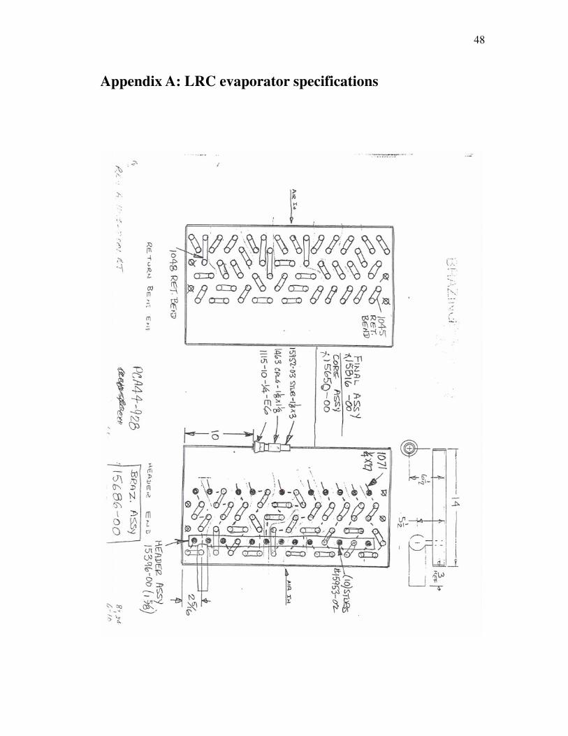
Appendix A: LRC evaporator specifications

49
50

51

52
Appendix B: Opto22 system and ICTD temperature probe
specifications
53
54
55
Appendix C: HOBO data logger specifications
56
57
Appendix D: Pressure transducer specifications

58
59
Appendix E: RTD sensor specifications
60
61
Appendix F: EES file for temperature model
"Determination of the relationship between temperature vs. time during the defrost" "Known Information for aluminum fin" rho_fin = 173 [lb/ft^3] "Assume density of the fin is constant
through out" thickness = 0.0003333333333 [feet] "This must change to feet" h_c = 0.88 [Btu/hr ft^2 F] "Using natural convection" T_amb = 35 [F] "Temperature of the room" Cp_fin = 0.21 [Btu/lbm*F] "Assume specific heat to be the same through out the fin" k_fin = 101 [Btu/hr*ft*F] "Assume Thermal conductivity to be the
same throughout the fin" T_hot_gas = 55 [F] "This takes into account of Q_in by knowing
boundary condition temperature" T_i = 35 [F] "Initial condition" "Known Information for copper tube wall" rho_copper = 557.7 [lb/ft^3] "Assume density of the copper is constant through out" h_R22 = 440.3 [Btu/h ft^2 F] "Using convection with phase change condensation" fin_pitch = 0.018 [feet] Cp_copper = 0.0906 [Btu/lbm*F] "Assume specific heat to be the same through out the copper" k_copper = 234 [Btu/hr*ft*F] "Assume Thermal conductivity to be the same through out the copper" "Radius of the copper tube" r_a = 0.025125 [feet] r_b = 0.026375 [feet] r_c = 0.027625 [feet]
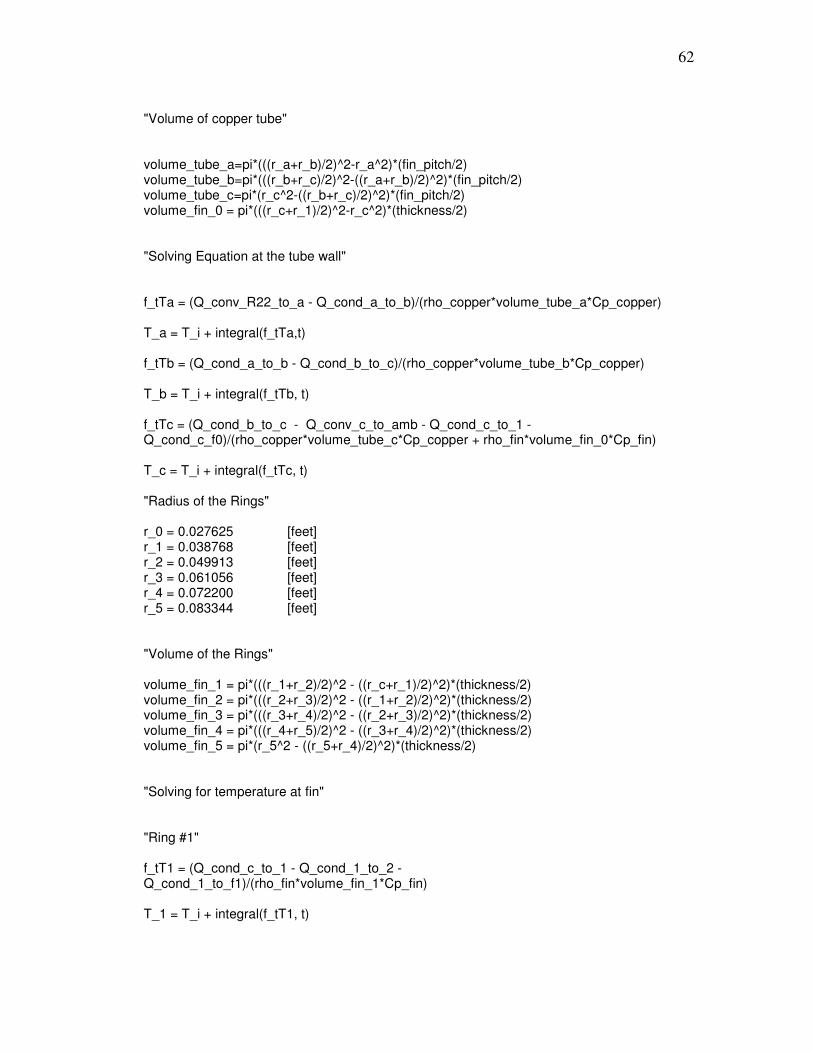
62
"Volume of copper tube" volume_tube_a=pi*(((r_a+r_b)/2)^2-r_a^2)*(fin_pitch/2) volume_tube_b=pi*(((r_b+r_c)/2)^2-((r_a+r_b)/2)^2)*(fin_pitch/2) volume_tube_c=pi*(r_c^2-((r_b+r_c)/2)^2)*(fin_pitch/2) volume_fin_0 = pi*(((r_c+r_1)/2)^2-r_c^2)*(thickness/2) "Solving Equation at the tube wall" f_tTa = (Q_conv_R22_to_a - Q_cond_a_to_b)/(rho_copper*volume_tube_a*Cp_copper) T_a = T_i + integral(f_tTa,t) f_tTb = (Q_cond_a_to_b - Q_cond_b_to_c)/(rho_copper*volume_tube_b*Cp_copper) T_b = T_i + integral(f_tTb, t) f_tTc = (Q_cond_b_to_c - Q_conv_c_to_amb - Q_cond_c_to_1 - Q_cond_c_f0)/(rho_copper*volume_tube_c*Cp_copper + rho_fin*volume_fin_0*Cp_fin) T_c = T_i + integral(f_tTc, t) "Radius of the Rings" r_0 = 0.027625 [feet] r_1 = 0.038768 [feet] r_2 = 0.049913 [feet] r_3 = 0.061056 [feet] r_4 = 0.072200 [feet] r_5 = 0.083344 [feet] "Volume of the Rings" volume_fin_1 = pi*(((r_1+r_2)/2)^2 - ((r_c+r_1)/2)^2)*(thickness/2) volume_fin_2 = pi*(((r_2+r_3)/2)^2 - ((r_1+r_2)/2)^2)*(thickness/2) volume_fin_3 = pi*(((r_3+r_4)/2)^2 - ((r_2+r_3)/2)^2)*(thickness/2) volume_fin_4 = pi*(((r_4+r_5)/2)^2 - ((r_3+r_4)/2)^2)*(thickness/2) volume_fin_5 = pi*(r_5^2 - ((r_5+r_4)/2)^2)*(thickness/2) "Solving for temperature at fin" "Ring #1" f_tT1 = (Q_cond_c_to_1 - Q_cond_1_to_2 - Q_cond_1_to_f1)/(rho_fin*volume_fin_1*Cp_fin) T_1 = T_i + integral(f_tT1, t)
63
"Ring #2" f_tT2 = (Q_cond_1_to_2 - Q_cond_2_to_3 - Q_cond_2_to_f2)/(rho_fin*volume_fin_2*Cp_fin) T_2 = T_i + integral(f_tT2, t) "Ring #3" f_tT3 = (Q_cond_2_to_3 - Q_cond_3_to_4 - Q_cond_3_to_f3)/(rho_fin*volume_fin_3*Cp_fin) T_3 = T_i + integral(f_tT3, t) "Ring #4" f_tT4 = ( Q_cond_3_to_4 - Q_cond_4_to_5 - Q_cond_4_to_f4)/(rho_fin*volume_fin_4*Cp_fin) T_4 = T_i + integral(f_tT4, t) "Ring #5" f_tT5 = (Q_cond_4_to_5 - Q_cond_5_to_f5)/(rho_fin*volume_fin_5*Cp_fin) T_5 = T_i + integral(f_tT5, t) "Solving for the frost Temperature" "Information about frost" k_frost = 1.283 [Btu/hr*ft*F] "Get the info from online: http://www.engineeringtoolbox.com/ice-thermal-properties-d_576.html" frost_thickness = 0.5*0.003281 [feet] "Convert from 1 milimeter of thickness" rho_frost = 18.7 [lb/ft^3] "Get the info from online: http://www.engineeringtoolbox.com/ice-thermal-properties-d_576.html" g_md = 0.000369 [lbm/ft^2 s] "Calculate from the mass transfer book by Mills page 53 to 54" m_H2O_s = 0.003745 "Calculate from the mass transfer book by Mills page 53 to 54" m_H2O_e = 0.003476 "Calculate from the mass transfer book by Mills page 53 to 54"
64
h_ig = 143.4 [Btu/lbm] “Enthalpy fusion of water” h_i = Enthalpy(Water,T=30,p=1) "Q_evap ring" Q_evap_0 = (g_md*pi*(((r_1 +r_c)/2)^2 - (r_c)^2)*(m_H2O_s - m_H2O_e)*h_ig) Q_evap_1 = (g_md*pi*(((r_2 +r_1)/2)^2 - ((r_1 + r_c)/2)^2)*(m_H2O_s - m_H2O_e)*h_ig) Q_evap_2 = (g_md*pi*(((r_3 +r_2)/2)^2 - ((r_2 + r_1)/2)^2)*(m_H2O_s - m_H2O_e)*h_ig) Q_evap_3 = (g_md*pi*(((r_4 +r_3)/2)^2 - ((r_3 + r_2)/2)^2)*(m_H2O_s - m_H2O_e)*h_ig) Q_evap_4 = (g_md*pi*(((r_5 +r_4)/2)^2 - ((r_4 + r_3)/2)^2)*(m_H2O_s - m_H2O_e)*h_ig ) Q_evap_5 = (g_md*pi*(r_5^2-((r_5+r_4)/2)^2)*(m_H2O_s - m_H2O_e)*h_ig ) "Frost ring" volume_frost_0 = pi*(((r_c+r_1)/2)^2 - (r_c)^2)*((fin_pitch/2)-(thickness/2)) volume_frost_1 = pi*(((r_1+r_2)/2)^2 - ((r_c+r_1)/2)^2)*frost_thickness volume_frost_2 = pi*(((r_2+r_3)/2)^2 - ((r_1+r_2)/2)^2)*frost_thickness volume_frost_3 = pi*(((r_3+r_4)/2)^2 - ((r_2+r_3)/2)^2)*frost_thickness volume_frost_4 = pi*(((r_4+r_5)/2)^2 - ((r_3+r_4)/2)^2)*frost_thickness volume_frost_5 = pi*(r_5^2 - ((r_5+r_4)/2)^2)*frost_thickness "Ring #0" f_th0 = (Q_cond_c_f0 - Q_conv_f0_to_amb - Q_cond_f0_to_f1 - Q_evap_0)/(rho_frost*volume_frost_0) h_f_0 = h_i + integral(f_th0,t) {T_f_0 = TEMPERATURE(Water,h=h_f_1,p=1)} T_f_0=Interpolate1('Lookup 1', 'T', 'h', h=h_f_0) "Ring #1" f_th1 = (Q_cond_f0_to_f1 - Q_conv_f1_to_amb - Q_cond_f1_to_f2 + Q_cond_1_to_f1 - Q_evap_1)/(rho_frost*volume_frost_1) h_f_1 = h_i + integral(f_th1,t) {T_f_1 = TEMPERATURE(Water,h=h_f_1,p=1)} T_f_1=Interpolate1('Lookup 1', 'T', 'h', h=h_f_1) "Ring #2" f_th2 = (Q_cond_f1_to_f2 - Q_conv_f2_to_amb - Q_cond_f2_to_f3 + Q_cond_2_to_f2 - Q_evap_2)/(rho_frost*volume_frost_2) h_f_2 = h_i + integral(f_th2,t) {T_f_2 = TEMPERATURE(Water,h=h_f_2,p=1)} T_f_2=Interpolate1('Lookup 1', 'T', 'h', h=h_f_2) "Ring #3"
65
f_th3 = (Q_cond_f2_to_f3 - Q_conv_f3_to_amb - Q_cond_f3_to_f4 + Q_cond_3_to_f3 - Q_evap_3)/(rho_frost*volume_frost_3) h_f_3 = h_i + integral(f_th3,t) {T_f_3 = TEMPERATURE(Water,h=h_f_3,p=1)} T_f_3=Interpolate1('Lookup 1', 'T', 'h', h=h_f_3) "Ring #4" f_th4 = (Q_cond_f3_to_f4 - Q_conv_f4_to_amb - Q_cond_f4_to_f5 + Q_cond_4_to_f4 - Q_evap_4)/(rho_frost*volume_frost_4) h_f_4 = h_i + integral(f_th4,t) {T_f_4 = TEMPERATURE(Water,h=h_f_4,p=1)} T_f_4=Interpolate1('Lookup 1', 'T', 'h', h=h_f_4) "Ring #5" f_th5 = (Q_cond_f4_to_f5 - Q_conv_f5_to_amb + Q_cond_5_to_f5 - Q_evap_5)/(rho_frost*volume_frost_5) h_f_5 = h_i + integral(f_th5,t) {T_f_5 = TEMPERATURE(Water,h=h_f_5,p=1)} T_f_5=Interpolate1('Lookup 1', 'T', 'h', h=h_f_5) "List of all the Heat energy terms" Q_conv_R22_to_a = (h_R22*pi*r_a*fin_pitch*(T_hot_gas - T_a))/3600 Q_CONV_R22_to_a_sum = integral(Q_conv_R22_to_a, t) Q_cond_a_to_b = (k_copper*pi*fin_pitch*(T_a-T_b)/ln(r_b/r_a))/3600 Q_COND_a_to_b_sum = integral(Q_cond_a_to_b, t) Q_cond_b_to_c = (k_copper*pi*fin_pitch*(T_b-T_c)/ln(r_c/r_b))/3600 Q_COND_b_to_c_sum = integral(Q_cond_b_to_c, t) Q_conv_c_to_amb = (h_c*pi*r_c*((fin_pitch)/2 - (thickness)/2 - frost_thickness)*(T_c-T_amb))/3600 Q_CONV_c_to_amb_sum = integral(Q_conv_c_to_amb , t) Q_cond_c_to_1 = (k_fin*pi*thickness*(T_c-T_1)/ln(r_1/r_c))/3600 Q_COND_c_to_1_sum = integral(Q_cond_c_to_1, t) Q_cond_c_f0 = (((2*pi*(((r_1+r_c)/2)^2-(r_c)^2)*(T_c - T_f_0)*(k_fin*k_frost))/((thickness*k_frost)+(2*frost_thickness*k_fin)))/3600) "+ ((k_frost*2*pi*(fin_pitch/2 - thickness/2)*(T_c - T_f_0)/LN(r_0/r_c))/3600)"
66
Q_COND_c_f0_sum = integral(Q_cond_c_f0,t) Q_cond_1_to_2 = (k_fin*pi*thickness*(T_1-T_2)/ln(r_2/r_1))/3600 Q_COND_1_to_2_sum = integral(Q_cond_1_to_2, t) Q_cond_1_to_f1 = ((2*pi*(((r_2+r_1)/2)^2-((r_1+r_c)/2)^2)*(T_1 - T_f_1)*(k_fin*k_frost))/((thickness*k_frost)+(2*frost_thickness*k_fin)))/3600 Q_COND_1_to_f1_sum = integral(Q_cond_1_to_f1, t) Q_cond_2_to_3 = (k_fin*pi*thickness*(T_2-T_3)/ln(r_3/r_2))/3600 Q_COND_2_to_3_sum = integral(Q_cond_2_to_3, t) Q_cond_2_to_f2 = ((2*pi*(((r_3+r_2)/2)^2-((r_2+r_1)/2)^2)*(T_2 - T_f_2)*(k_fin*k_frost))/((thickness*k_frost)+(2*frost_thickness*k_fin)))/3600 Q_COND_2_to_f2_sum = integral(Q_cond_2_to_f2 , t) Q_cond_3_to_4 = (k_fin*pi*thickness*(T_3-T_4)/ln(r_4/r_3))/3600 Q_COND_3_to_4_sum = integral(Q_cond_3_to_4, t) Q_cond_3_to_f3 = ((2*pi*(((r_4+r_3)/2)^2-((r_3+r_2)/2)^2)*(T_3 - T_f_3)*(k_fin*k_frost))/((thickness*k_frost)+(2*frost_thickness*k_fin)))/3600 Q_COND_3_to_f3_sum = integral(Q_cond_3_to_f3, t) Q_cond_4_to_5 = (k_fin*pi*thickness*(T_4-T_5)/ln(r_5/r_4))/3600 Q_COND_4_to_5_sum = integral(Q_cond_4_to_5, t) Q_cond_4_to_f4 = ((2*pi*(((r_5+r_4)/2)^2-((r_4+r_3)/2)^2)*(T_4 - T_f_4)*(k_fin*k_frost))/((thickness*k_frost)+(2*frost_thickness*k_fin)))/3600 Q_COND_4_to_f4_sum = integral(Q_cond_4_to_f4, t) Q_cond_5_to_f5 = ((2*pi*((r_5)^2-((r_5+r_4)/2)^2)*(T_5 - T_f_5)*(k_fin*k_frost))/((thickness*k_frost)+(2*frost_thickness*k_fin)))/3600 Q_COND_5_to_f5_sum = integral(Q_cond_5_to_f5, t) Q_cond_f0_to_f1 = (k_frost*2*pi*frost_thickness*(T_f_0 - T_f_1)/LN(r_1/r_0))/3600 Q_COND_f0_to_f1_sum = integral(Q_cond_f0_to_f1, t) Q_conv_f0_to_amb = (h_c*pi*(((r_1+r_c)/2)^2-(r_c)^2)*(T_f_0 -T_amb))/3600 + ((h_c*pi*(r_1+r_c)/2)*((fin_pitch/2) - (thickness/2) - frost_thickness)*(T_f_0 - T_amb))/3600 Q_CONV_f0_to_amb_sum = integral(Q_conv_f0_to_amb,t) Q_conv_f1_to_amb = (h_c*pi*(((r_2+r_1)/2)^2-((r_1+r_c)/2)^2)*(T_f_1 -T_amb))/3600 Q_CONV_f1_to_amb_sum = integral(Q_conv_f1_to_amb, t)
67
Q_cond_f1_to_f2 = (k_frost*2*pi*frost_thickness*(T_f_1-T_f_2)/LN(r_2/r_1))/3600 Q_COND_f1_to_f2_sum = integral(Q_cond_f1_to_f2, t) Q_conv_f2_to_amb = (h_c*pi*(((r_3+r_2)/2)^2-((r_2+r_1)/2)^2)*(T_f_2 -T_amb))/3600 Q_CONV_f2_to_amb_sum = integral(Q_conv_f2_to_amb, t) Q_cond_f2_to_f3 = (k_frost*2*pi*frost_thickness*(T_f_2-T_f_3)/LN(r_3/r_2))/3600 Q_COND_f2_to_f3_sum = integral(Q_cond_f2_to_f3, t) Q_conv_f3_to_amb = (h_c*pi*(((r_4+r_3)/2)^2-((r_3+r_2)/2)^2)*(T_f_3 -T_amb))/3600 Q_CONV_f3_to_amb_sum = integral(Q_conv_f3_to_amb, t) Q_cond_f3_to_f4 = (k_frost*2*pi*frost_thickness*(T_f_3-T_f_4)/LN(r_4/r_3))/3600 Q_COND_f3_to_f4_sum = integral(Q_cond_f3_to_f4, t) Q_conv_f4_to_amb = (h_c*pi*(((r_5+r_4)/2)^2-((r_4+r_3)/2)^2)*(T_f_4 -T_amb))/3600 Q_CONV_f4_to_amb_sum = integral(Q_conv_f4_to_amb, t) Q_cond_f4_to_f5 = (k_frost*2*pi*frost_thickness*(T_f_4-T_f_5)/LN(r_5/r_4))/3600 Q_COND_f4_to_f5_sum = integral(Q_cond_f4_to_f5, t) Q_conv_f5_to_amb = (h_c*pi*(r_5^2-((r_5+r_4)/2)^2)*(T_f_5 -T_amb))/3600 Q_CONV_f5_to_amb_sum = integral(Q_conv_f5_to_amb, t) Q_conv = (h_c*pi*r_c*(fin_pitch-thickness)*(T_c-T_amb) + h_c*pi*(((r_2+r_1)/2)^2-((r_1+r_c)/2)^2)*(T_f_1 -T_amb) + h_c*pi*(((r_3+r_2)/2)^2-((r_2+r_1)/2)^2)*(T_f_2 -T_amb) + h_c*pi*(((r_4+r_3)/2)^2-((r_3+r_2)/2)^2)*(T_f_3 -T_amb) + h_c*pi*(r_5^2-((r_5+r_4)/2)^2)*(T_f_5 -T_amb) + h_c*pi*(r_5^2-((r_5+r_4)/2)^2)*(T_f_5 -T_amb))/3600 Q_CONV_TOTAL = integral(Q_conv, t) Q_evap_sum = (Q_evap_1 + Q_evap_2 + Q_evap_3 + Q_evap_4 + Q_evap_5) Q_EVAP_TOTAL = integral(Q_evap_sum, t) Q_in = (h_R22*pi*r_a*fin_pitch*(T_hot_gas - T_a))/3600 Q_IN_TOTAL = integral(Q_in, t) Q_tube=rho_copper*volume_tube_a*Cp_copper*(T_a-T_i)+rho_copper*volume_tube_b*Cp_copper*(T_b-T_i)+rho_copper*volume_tube_c*Cp_copper*(T_c-T_i) Q_fin=rho_fin*volume_fin_0*Cp_fin*(T_c-T_i)+rho_fin*volume_fin_1*Cp_fin*(T_1-T_i)+rho_fin*volume_fin_2*Cp_fin*(T_2-T_i)+rho_fin*volume_fin_3*Cp_fin*(T_3-T_i)+rho_fin*volume_fin_4*Cp_fin*(T_4-T_i)+rho_fin*volume_fin_5*Cp_fin*(T_5-T_i)
68
Q_melt=rho_frost*volume_frost_0*(h_f_0-h_i)+rho_frost*volume_frost_1*(h_f_1-h_i)+rho_frost*volume_frost_2*(h_f_2-h_i)+rho_frost*volume_frost_3*(h_f_3-h_i)+rho_frost*volume_frost_4*(h_f_4-h_i)+rho_frost*volume_frost_5*(h_f_5-h_i) Q_Total=Q_tube+Q_fin+Q_melt+Q_evap_total+Q_conv_total ratio=Q_total/(Q_in_total+.0000000001) eff = Q_melt/(Q_in_total+.0000000001) number_elements = 70000 Cost = 0.1*((Q_IN_TOTAL*(1- eff))/3)*(number_elements/3412)
69
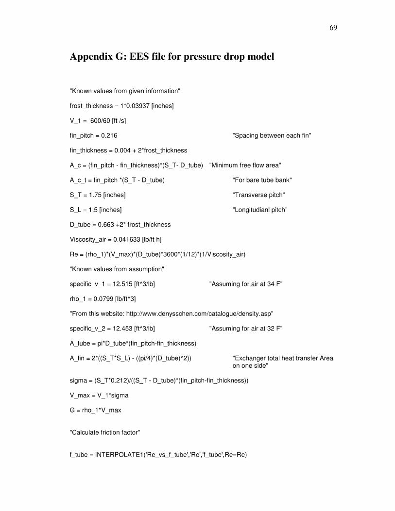
Appendix G: EES file for pressure drop model
"Known values from given information" frost_thickness = 1*0.03937 [inches] V_1 = 600/60 [ft /s] fin_pitch = 0.216 "Spacing between each fin" fin_thickness = 0.004 + 2*frost_thickness A_c = (fin_pitch - fin_thickness)*(S_T- D_tube) "Minimum free flow area" A_c_t = fin_pitch *(S_T - D_tube) "For bare tube bank" S_T = 1.75 [inches] "Transverse pitch" S_L = 1.5 [inches] "Longitudianl pitch" D_tube = 0.663 +2* frost_thickness Viscosity_air = 0.041633 [lb/ft h] Re = (rho_1)*(V_max)*(D_tube)*3600*(1/12)*(1/Viscosity_air) "Known values from assumption" specific_v_1 = 12.515 [ft^3/lb] "Assuming for air at 34 F" rho_1 = 0.0799 [lb/ft^3] "From this website: http://www.denysschen.com/catalogue/density.asp" specific_v_2 = 12.453 [ft^3/lb] "Assuming for air at 32 F" A_tube = pi*D_tube*(fin_pitch-fin_thickness) A_fin = 2*((S_T*S_L) - ((pi/4)*(D_tube)^2)) "Exchanger total heat transfer Area
on one side" sigma = (S_T*0.212)/((S_T - D_tube)*(fin_pitch-fin_thickness)) V_max = V_1*sigma G = rho_1*V_max "Calculate friction factor" f_tube = INTERPOLATE1('Re_vs_f_tube','Re','f_tube',Re=Re)
70
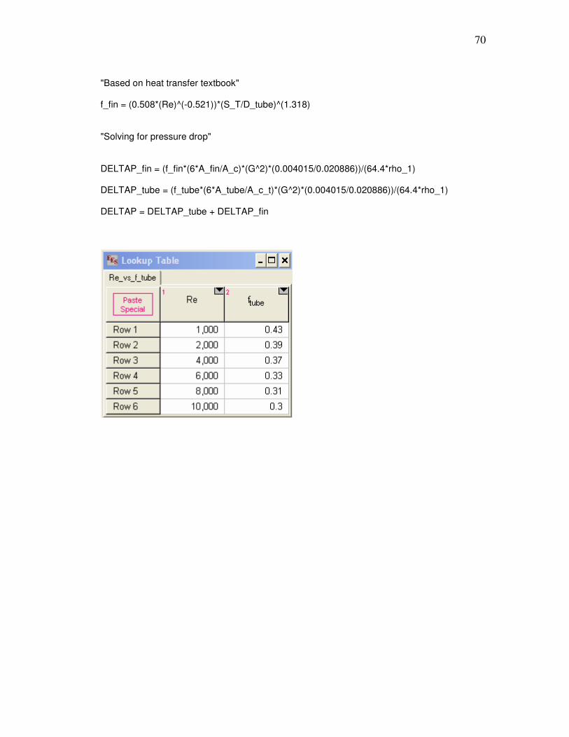
"Based on heat transfer textbook" f_fin = (0.508*(Re)^(-0.521))*(S_T/D_tube)^(1.318) "Solving for pressure drop" DELTAP_fin = (f_fin*(6*A_fin/A_c)*(G^2)*(0.004015/0.020886))/(64.4*rho_1) DELTAP_tube = (f_tube*(6*A_tube/A_c_t)*(G^2)*(0.004015/0.020886))/(64.4*rho_1) DELTAP = DELTAP_tube + DELTAP_fin
71
Appendix H: Weather data during experiment
Copyright © 2022 FDOKUMEN

