


Bahasa
Halaman
Hukum


IZA DP No. 2358
Conjugal Bereavement Effects on Healthand Mortality at Advanced Ages
Gerard J. van den BergMaart en LindeboomFrance Port rait
DI
SC
US
SI
ON
P
AP
ER
S
ER
IE
S
Forschungsinst it ut
zur Zukunf t der Arbeit
Inst it ut e for t he St udy
of Labor
Oct ober 2006

Conjugal Bereavement Effects on Health and Mortality at Advanced Ages
Gerard J. van den Berg Free University Amsterdam, IFAU Uppsala,
CEPR, IFS, Netspar and IZA Bonn
Maarten Lindeboom
Free University Amsterdam, HEB Bergen, Netspar and IZA Bonn
France Portrait
Free University Amsterdam
Discussion Paper No. 2358 October 2006
IZA
P.O. Box 7240 53072 Bonn
Germany
Phone: +49-228-3894-0 Fax: +49-228-3894-180
E-mail: [email protected]
Any opinions expressed here are those of the author(s) and not those of the institute. Research disseminated by IZA may include views on policy, but the institute itself takes no institutional policy positions. The Institute for the Study of Labor (IZA) in Bonn is a local and virtual international research center and a place of communication between science, politics and business. IZA is an independent nonprofit company supported by Deutsche Post World Net. The center is associated with the University of Bonn and offers a stimulating research environment through its research networks, research support, and visitors and doctoral programs. IZA engages in (i) original and internationally competitive research in all fields of labor economics, (ii) development of policy concepts, and (iii) dissemination of research results and concepts to the interested public. IZA Discussion Papers often represent preliminary work and are circulated to encourage discussion. Citation of such a paper should account for its provisional character. A revised version may be available directly from the author.

IZA Discussion Paper No. 2358 October 2006
ABSTRACT
Conjugal Bereavement Effects on Health and Mortality at Advanced Ages*
We specify a model for the lifetimes of spouses and the dynamic evolution of health, allowing spousal death to have causal effects on the health and mortality of the survivor. We estimate the model using a longitudinal survey that traces many health status aspects over time, and that is linked to register data on the vital status of the individuals. The model takes account of selectivity in partners' mortality and health evolution. We find strong instantaneous effects of bereavement on mortality and on certain aspects of health. Individuals lose on average 12 % of residual life expectancy after bereavement. Bereavement affects the share of healthy years in residual lifetime, primarily because healthy years are replaced by years with chronic diseases. JEL Classification: I12, I11, J14, J12, C41 Keywords: death, longevity, health care, disease, life expectancy, elderly couples,
impairment Corresponding author: Gerard J. van den Berg Department of Economics Free University of Amsterdam De Boelelaan 1105 1081 HV Amsterdam The Netherlands E-mail: [email protected]
* We thank participants in workshops and conferences in Bergen, York, Amsterdam, The Hague, Lund, Tunis, Venice, and Bonn, in particular Dan Hamermesh, for useful comments. Part of the research was carried out when Lindeboom was Visiting Professor at the Department of Economics and the ISR at the University of Michigan, Ann Arbor, USA. The Longitudinal Aging Study Amsterdam (LASA) kindly allowed us to use their LASA survey data. LASA has been supported by a long term grant from the Netherlands Ministry of Health, Welfare and Sports.
1 Introduction
At high ages, dramatic events in an individual’s life may lead to dramatic changes
in his or her health conditions. In particular, the death of the spouse can be a
major sources of psychosocial stress, depression and anxiety. These are all fac-
tors associated with morbidity and mortality.1 Conjugal bereavement may also
directly deteriorate physical health, for instance by impairing the immune sys-
tem, increasing the prevalence of chronic illnesses, and functional limitations.
Furthermore, most older widowers experience (serious) difficulties in performing
housekeeping chores like cooking or cleaning. This may in the long run negatively
affect their health - due, for instance, to insufficient caloric intake or nutritional
deficits. Finally, there is evidence that widows often suffer from greater poverty,
a factor associated with higher morbidity and mortality among the aged.2 Os-
terweis, Solomon and Green (1984) provide a detailed overview of the possible
causal effects of bereavement on health and mortality.
Conjugal bereavement affects the potential supply of informal care for the
person left behind (the non-organized care provided from within the social net-
work of the individual). Informal care is an essential supplement or substitute to
self-care and professional long-term care. In the Netherlands for instance, about
30% of older (65 plus) individuals receive some kind of informal assistance (see
e.g. Portrait, 2000). The larger part of the informal assistance is provided by
healthier partners (see for instance Norton, 2000, and Lakdawalla and Philipson,
2002). This is reflected in health care costs. Prigerson, Maciejewski and Rosen-
heck (2000) estimated average health costs in 1989 and find that costs equal
$ 2,384 for widowed and $ 1,498 for married subjects. So, if the death of the
partner negatively affects the health and well-being of the surviving spouse, it
also reduces the supply of informal care whereas in fact the demand for care has
increased (see Williams, 2004, for additional evidence). This will exacerbate the
health effects and therefore increase the demand for formal health care services
use, and this increases health care costs.
In this paper we provide a detailed analysis of health and mortality risks at
advanced ages. We model the dynamic evolution of health and we focus on the
effect of conjugal bereavement on health and mortality risks. This enables us to
improve on the existing literature in two ways. First, note that the lifetimes of
spouses may be related because of a causal effect of the death of one member
on the mortality rate of the surviving spouse, or because of (unobserved) fac-
1See for instance Prigerson, Maciejewski and Rosenheck (2000).2See for instance Ecob and Smith (1999) and Benzeval and Judge (2001).
2

tors that influence both lifetimes. With respect to the latter, spouses may have
similar health-related behavior, eating patterns, material circumstances, marital
satisfaction, or more generally, spouses have shared life histories that may af-
fect husband-wife mortality and morbidity. Klein (1992) finds that death times
are related significantly between husbands and wives through unobserved couple-
level frailty. This means that there may be a stochastic relationship between the
two lifetimes, even after we have controlled for observed characteristics. It also
means that we can not simply assume that the vital status of one spouse is an
exogenous determinant of the mortality rate of the other. Instead we model the
lifetimes of both spouses and the multiple ways in which they are related. This
distinguishes our model from the usual contributions on conjugal bereavement ef-
fects. One major exception is Lichtenstein et al. (1998) in which the dependence
of survival status on marital status is studied using twin data. They assume that
there is an identical unobserved component for both members of the twin couple
and use stratified partial likelihood methods to assess the causal effect of spousal
bereavement on subsequent mortality.
Furthermore, the large majority of the studies in this area analyze the effect of
bereavement on one specific aspect of health status, like stress or mortality.3 This
includes Lichtenstein et al. (1998) who restrict attention to mortality. A second
main contribution of our study is that we distinguish between different aspects
of health. There are large differences in health status among the aged. Some of
them are healthy, whereas others suffer from cognitive impairment, but are in
perfect physical condition, and yet others combine cognitive impairment with
severe physical limitations. We consider all of these and study their simultaneous
dynamic evolution.
Our analyzes are based on a dataset covering about 2,000 older couples for the
period 1992-2000 called the Longitudinal Aging Study Amsterdam. The dataset
has abundant information on health indicators and outcomes as well as on socio-
demographic variables. Of interest for our analyses is that about 24% of the main
3See, for instance, Prigerson, Maciejewski and Rosenheck (2000) and Dijkstra, Van Tilburg
and De Jong Gierveld (2005) on the effect on psychosocial stress, depression, anxiety and lone-
liness, Irwin et al. (1987, 1993) on impaired immune function, Prigerson et al. (1997, 2000)
on chronic illnesses and functional limitations, Koehn (2001) on caloric intake and nutritional
deficits, and McGarry and Schoeni (2005) on poverty. Lillard and Panis (1996) study mortality
outcomes and incorporate a one-dimensional self-reported general-health assessment into the
analysis. This health variable is observed at regular time intervals. They also control for related
unobserved determinants in marital status, health, and mortality. However, the empirical anal-
ysis focuses on the effect of marital status (formation and dissolution) in general on mortality,
and most observed dissolutions are not bereavements but divorces.
3

respondents and about 17.3 % of their partners are observed to die during the
period of observation, and that we were able to obtain administrative data on
the vital status of the respondents and of their spouse for the entire period of
observation.
The information in the data allows us to carefully characterize health evolu-
tion, to examine how health status influences mortality, to model the interrelation
between the lifetimes of spouses, and to study how the death of a partner influ-
ences the health and mortality of the surviving spouse. As will be explained,
feasibility constraints demand the use of a data reduction method to summarize
the observed health information in an equally informative health set of lower
dimension. We use a flexible non-parametric method called the Grade of Mem-
bership Method (GoM) (Woodbury and Clive, 1974; Woodbury and Manton,
1982). This method is designed to summarize a large set of health conditions
into a smaller number of clinical disease types. It is particularly useful if the
observable health-condition outcome variables are binary or only have a small
set of possible values. The method also determines individual weights measuring
the degree to which an individual fits each of the clinical disease types. We use
these Grade of Membership individual weights as measures for the health status
of the respondents and include these as regressors in our model for mortality.
These health measures are likely to be endogenous and we therefore extend our
bivariate survival model with a model for health dynamics. Health is allowed to
depend on lagged health, individual characteristics and the death of the partner.
We use the estimated model to calculate expected residual lifetimes in dif-
ferent health states (“health expectancies”) for married and widowed males and
females of various age groups. Health expectancies are informative on the frac-
tion of life spent in a healthy state compared to the fraction spent in frail health
conditions. This information plays a central role in the policy debate about the
future needs for long-term care of older populations. For a recent review on health
expectancies, see Robine, Jagger, and Mathers (2003).
Section 2 reports on the dataset. Section 3 discusses the non-parametric Grade
of Membership method. We apply the method on our data and briefly discuss
the main results. Section 4 proceeds with the statistical model for health and
mortality and Section 5 presents the results. In Section 6 we present the results of
simulations with the model. In particular, we compare expected residual lifetimes
and health expectancies of married and bereaved individuals. Section 7 concludes.
4

2 Data
We use data from the Longitudinal Aging Study Amsterdam (LASA) (Deeg,
Knipscheer and Van Tilburg, 1993). The LASA study follows over time a rep-
resentative sample of non-institutionalized and institutionalized individuals aged
55 and above. The respondents lived at baseline (1992) in 11 municipalities in
the West, North-East, and South of the Netherlands. We use three waves: the
1992-93 wave, the 1995-96 wave, and the 1998-99 wave.4 Apart from the usual
socio-demographic variables, this dataset provides extensive information on the
physical, emotional, mental, and social functioning and also on a large set of
variables that may have an effect on these four aspects of functioning. Each com-
ponent is assessed by questionnaires and tests. Individuals were submitted either
to a complete face-to-face interview or, if they refused this, to a short telephone
interview.
The LASA dataset is linked to administrative records on the vital and marital
status of the main respondents and their spouses up to the first of January 2000.
If the respondent died during the sampling period, the date and place of death
as well as the timing of spousal bereavement (if he or she was widowed at the
moment of death) are recorded. For respondents who are still alive at the first of
January 2000, changes in marital status – and the moment these changes took
place – are also registered. This allows us to accurately follow the changes in
marital and vital status from the start of the sampling period up to the first of
January 2000. The smallest interval of time between deaths of spouses is 20 days
and one quarter of the respondents observed to die after conjugal bereavement
die within one year.
There are however some data limitations. First, information on the spouse
is not available after the death of the LASA respondent. Second, for privacy
reasons, the municipality of Amsterdam refused to provide records on spouses.
Consequently, the information on the vital status of spouses of respondents who
lived in Amsterdam can only be obtained from the survey data. We return to
factual numbers concerning this below.
2,061 individuals share their household with a partner at the initial wave in
1992. Respondents who lost their partner before this initial wave are excluded.
For this group we do not have information on the partner. We also excluded
a small group (121) of people living together but who were not married. For
4The LASA respondents are drawn from a dataset on social network of older individuals
held in the early months of 1992. This dataset, called the LSN dataset (Van Tilburg et al.
1992), provides among other things the household history of the respondents.
5

this group we lacked essential information on the vital status of the partner.5
Respondents who were still legally married but who were not living together (13
individuals) were also excluded from our dataset. 6 respondents are observed
to divorce during the observation period; these respondents are discarded from
our analyses as well. The resulting sample counts 1.921 individuals. Very few
respondents (about 0.3% of our sample) are observed to re-marry after a period
of widowhood. We decided to only use the information of these individuals up to
the time of their new marriage.
Figure 1 shows the evolution of marital status and mortality over time. About
24 % of the main respondents died during the sample period. This concerns 345
males (dying at an average age of 79) and 111 females (dying at an average age of
78). 269 respondents were still married at the time of their death. 37 males and
25 males were observed to die after a period of widowhood (on average 2.2 and
2.9 years for respectively males and females). The remaining 125 (345 + 111 - 269
- 37 - 25) respondents who are observed to die lived in the city of Amsterdam.
For these 125 respondents we can only assess their marital status from survey
information. More precisely, information on the vital status of the spouse can
only be obtained for these respondents if they lived longer than their spouse and
also participated in a wave after the death of their partner. We furthermore have
256 respondents from Amsterdam, who were still alive at the first of January of
2000. For these individuals, we miss information on the vital status of the spouse
for the period between their last interview and the first of January 2000. These
partial observability problems need to be accounted for in the construction of the
likelihood function. We return to this in Section 4.
In total we observe 331 cases where the partner of the main respondent dies
(116 widowers and 215 widows). The average ages of widowhood are equal to
78.4 for males and 73.4 for females. Figure 2 shows the survival curve based on
the Kaplan-Meier estimate of the mortality hazard. First, it should be noted that
the survival probabilities for married individuals who are older then 86 are based
on a small number of observations. The same is true for age class 49-55. Second,
the graph shows that the survival probabilities are lower for widowed individuals,
except at older ages. For younger ages there is a relatively large difference between
the curves for married individuals and widowed individuals. This is consistent
with the results in the literature on mortality and spousal bereavement (see, for
instance, Lichtenstein et al. 1998).
5The cause of a separation between unmarried partners (death, discord, hospitalization,
admission in nursing or residential homes etc.) is not recorded in the LASA study. Moreover,
municipalities only provide records of official partners – i.e. spouses.
6

Figure 1: Evolution of marital status during the LASA study
92/93
95/96
2000
98/99
1516 married
respondents
1233 married
respondents
1921 married respondents
160 widowed
220 deceasedrespondents:- 14 widowed- 149 married- 57 with unknownmarital status*
132 deceasedrespondents:- 6 widowed - 81 married- 45 with unknown marital status*
27 deceasedrespondents
127widowed
133 widowed
8 deceasedrespondents
6 deceasedrespondents
50 deceased respondents:- 1 widowed- 39 married- 10 with unknownmarital status*
1183 survivors:- 23 widowed- 940 married- 220 withunknownmarital status*
25 survivorswith unknownmarital status*
24 withunknownmaritalstatus*
13 deceasedrespondents
* Individuals registrered in Amsterdam
7

Figure 2: Kaplan-Meier survivor function
Kaplan-Meier survivor function
0
0.1
0.2
0.3
0.4
0.5
0.6
0.7
0.8
0.9
1
55 68 80 91
Age
Sur
vivo
r pro
bab
ility
MarriedWidowed at age 55-65Widowed at age 65-75Widowed at age 75-85
8

Health status is a crucial variable in our model. Health is a multidimensional
concept and especially at advanced ages, striking differences are observed be-
tween individuals as well as over time. We use an extensive set of 22 health
measures that each describe different aspects of health, but together provide a
complete picture of health.6 Physical functioning is measured by a self-reported
test on mobility (van Sonsbeek 1988) and by a performance test of physical abil-
ity (Gulranik, 1994). Cognitive status is assessed using the Mini Mental State
Examination (MMSE, Folstein, 1975). The Center for Epidemiologic Studies De-
pression Scale (CES-D, Radloff, 1977) is used to measure emotional functioning of
older individuals. Two self-reported items on difficulties with seeing and hearing
measure perception. Finally, the presence of chronic diseases is assessed by ask-
ing the participants whether they have or have had any of the following diseases:
chronic obstructive pulmonary diseases (COPD), heart diseases, atherosclerosis,
stroke, diabetes, arthritis, cancer, and other chronic diseases. These diseases are
the most prevalent ones in older persons. To assess the severity of each disease,
it is asked whether respondents follow a medical treatment. Unfortunately, the
information on health is only available for the head respondent, and not for the
spouse.7
A problem with the high dimensionality of the health data is that it will be
difficult to use these indicators simultaneously in an empirical model for health
and mortality. In Section 3, we discuss a flexible non-parametric data reduction
method called the Grade of Membership method. Before we do this, we first
briefly list socio-demographic variables that we will use in our analyzes.
Income is derived from a question where respondents were asked to assign
their monthly total income - derived from pension, savings, dividends, and other
sources - to four categories (in $): 0 - 794 (in line with the Dutch minimum in-
come), 795 - 1,134, 1,134 - 1,815 and more than 1,815.8 For the spouse, we use as
proxy for income the occupational prestige of the longest job according to Sixma
and Ultee (1983) (ranging from 0 = “never had job” until 87 = “high prestige”).
A categorical variable indicating the level of education attained is used as a sup-
plemental measure of socioeconomic status and is determined by the question:
“Which is the highest education level attained?” Nine categories were reported
6The 22 health measures have been selected in collaboration with gerontologists and epi-
demiologists.7This will of course affect our empirical model. We return to this issue in Section 4.8Missing values for income were relatively frequent (almost 15%) and were imputed on the
basis of results of regression analyses of income on demographic and socioeconomic variables
such as age, cohort, gender, education, and degree of urbanization of the municipality where
the respondent lives.
9

varying from “elementary education not completed” to “university education”.
The degree of urbanization of the area where the respondent lives (categorical
variable ranging from 1 = “low” until 10 =“high”) is an indicator of the external
living conditions and may influence positively or negatively the probabilities of
dying of older individuals through a variety of mediating factors – such as feelings
of insecurity, pollution, and availability of both formal and informal caregivers.
The variable “network size” (Van Tilburg et al. 1992) indicates the number of
network members – including children, other family members, friends, and neigh-
bors – who have regular contacts with the main respondent. The size of the social
network may affect morbidity or mortality in different ways. Previous studies in-
dicate that having children is one of the best predictors of formal and informal
care (Norton 2000). Our network variable includes this. We opted for the variable
“network size” instead of a set of variables measuring the number and gender of
children because “network size” excludes children with whom older individuals do
not have any contact, or who do not support their parents. A variable indicating
the frequency of church attendance is included in our analyses. The strength of
church affiliation may give some information on the lifestyle of the respondent,
and also on the way the respondent deals with the bereavement process. The
variable takes on value 0 if the respondent does not go to any church and ranges
from value 1 (“yearly or less”) until 5 (“weekly or more”). We also include age
and gender.
The quality of marital union may affect the way widowed individuals adjust
to the loss of the spouse (see for instance Van Baarsen and Broese van Groenou,
2001, Prigerson et al., 2000). Unfortunately, no reliable information on marital
satisfaction is available in the data set. The duration of the marital union is
included in the analyses as a proxy for the quality of marriage.9
Table 1 below presents the means of the demographic and socio-economic
variables.
9We will allow for time constant unobserved individual components in our model. This will
account for the average quality of the marriage.
10

Table 1: Demographic and socioeconomic characteristics of the head (Wave I)
Variables Score Wave I (in %)
Number of individuals 1,743
Female 41.5
Age 55-65 43
65-75 33.5
75-85 23.4
Attained education level respondent Low 58.1
Medium 27.6
Income in $ < 793 14.4
793-1134 37.0
1134-1815 32.7
Degree of Urbanization Low 14.0
Medium 29.4
Church attendance ≤ Yearly 45.6
Monthly 10.6
3 The Grade of Membership method
3.1 General description
To describe the health condition of older individuals, a broad range of different
measures is required to cover all dimensions of health. Above we discussed the
set of 22 measures that we use in our study. As we aim to analyze the dynamics
in health, we need a method that summarizes this extensive set of indicators into
a manageable and meaningful health set of lower dimension. In addition, this
data reduction method also needs to be as flexible as possible, given the complex
nature of health and the way it is distributed across individuals in the sample.
The Grade of Membership (GoM) method is perfectly suited for this.
The GoM, developed by Woodbury and Clive (1974), Woodbury, Clive and
Garson (1978), and Woodbury and Manton (1982), is a statistical classification
procedure, designed to summarize a complex set of symptoms for chronic diseases
into a smaller number of ideal clinical disease types. These ideal clinical disease
types are referred to as “pure types” in the GoM terminology. The method not
only makes a partitioning of the data into a limited set of pure types, but it also
provides for each individual in the sample different weights indicating the degree
of similarity that an individual has with each of the pure types. These weights,
called “grades of membership”, sum up to unity over the classes. A weight of
1.0 means that an individual has all of the symptoms associated with the pure
type (so this individual can be viewed as a “standard textbook case”), whereas
11
a weight of 0.0 indicates that the individual bears no similarities with the pure
type at all. The method is similar to the well known and much applied factor
analysis, but it has some distinctive properties that are particularly relevant for
our study. We return to this after a more formal description of the method.
3.2 The method
Suppose that there are K underlying non overlapping pure (clinical disease) types.
Suppose furthermore that we have access to a set of J variables or tests that
together cover the symptoms of the underlying pure types present in a sample
of I individuals. As the information in each test j can have multiple response
categories, Lj, we can without loss of information code the test score of individual
i in test j into a set of dichotomous indicators yijl, measuring whether or not
individual i has responded or scored affirmative on the lth outcome of test j.
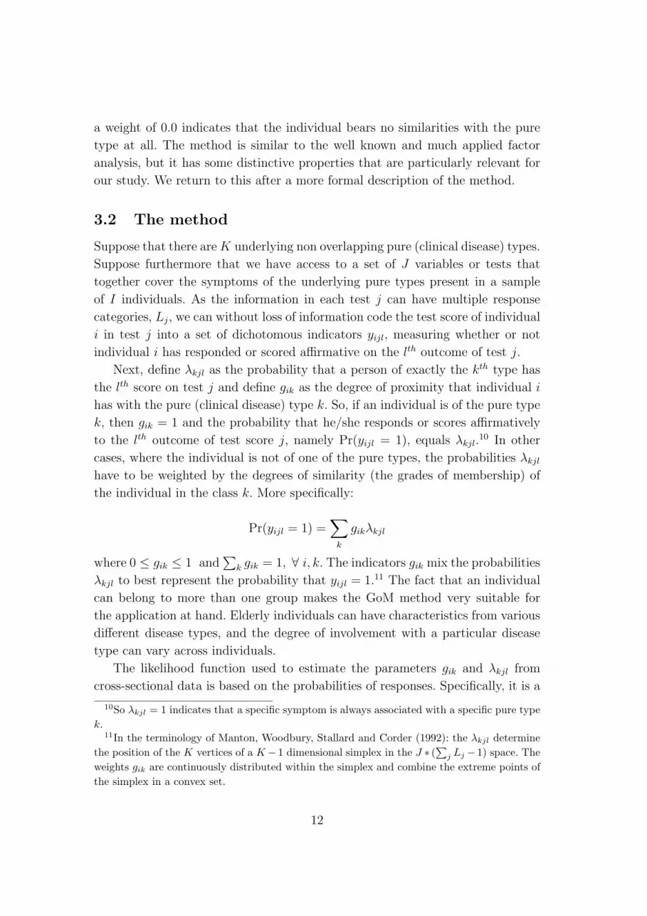
Next, define λkjl as the probability that a person of exactly the kth type has
the lth score on test j and define gik as the degree of proximity that individual i
has with the pure (clinical disease) type k. So, if an individual is of the pure type
k, then gik = 1 and the probability that he/she responds or scores affirmatively
to the lth outcome of test score j, namely Pr(yijl = 1), equals λkjl.10 In other
cases, where the individual is not of one of the pure types, the probabilities λkjl
have to be weighted by the degrees of similarity (the grades of membership) of
the individual in the class k. More specifically:
Pr(yijl = 1) =∑
k
gikλkjl
where 0 ≤ gik ≤ 1 and∑
k gik = 1, ∀ i, k. The indicators gik mix the probabilities
λkjl to best represent the probability that yijl = 1.11 The fact that an individual
can belong to more than one group makes the GoM method very suitable for
the application at hand. Elderly individuals can have characteristics from various
different disease types, and the degree of involvement with a particular disease
type can vary across individuals.
The likelihood function used to estimate the parameters gik and λkjl from
cross-sectional data is based on the probabilities of responses. Specifically, it is a
10So λkjl = 1 indicates that a specific symptom is always associated with a specific pure type
k.11In the terminology of Manton, Woodbury, Stallard and Corder (1992): the λkjl determine
the position of the K vertices of a K − 1 dimensional simplex in the J ∗ (∑
j Lj − 1) space. The
weights gik are continuously distributed within the simplex and combine the extreme points of
the simplex in a convex set.
12

simple independent multinomial given by:
L =∏
i
∏
j
∏
l
Pr(yijl = 1)yijl =∏
i
∏
j
∏
l
(∑
k
gikλkjl)yijl
This needs to be optimized with respect to gik and λkjl subject to the constraints:
0 ≤ gik ≤ 1 ∀ i, k∑
k
gik = 1
0 ≤ λkjl ≤ 1 ∀ k, j, l∑
l
λkjl = 1
As in Woodbury and Manton (1982), we use approximate likelihood ratio
tests for the determination of the order K (number of dimensions) of the model.
The test statistic is approximately χ2 distributed with the number of degrees
of freedom equal to the number of respondents I minus one plus the number of
variables j multiplied by the number of category per variable∑
j Lj. We refer to
Woodbury and Manton (1982) for more details.
Given K, we need to address the consistency of the estimates of the indi-
vidual parameters gik, not in the least because we use the estimated individual
parameters gik in subsequent analyzes of health dynamics and mortality (Section
4). For consistency of gik, we have to rely on information growth in J or Lj.
More specifically, consistency is ensured when J ∗ (Lj − 1) becomes large (see,
for instance, Manton, Woodbury, Stallard and Corder, 1992). In our application
J ∗ (Lj − 1) equals 25, which may be sufficient, for not too large K, to accurately
estimate the individual parameters gik.
The GoM approach is similar to factor analysis. The factor loadings compare
to λkjl, whereas the gik have a similar function as the factor scores. However,
factor analysis typically makes distributional (normal) assumptions on the factor
scores and the outcomes, whereas the GoM method requires no assumption on
the distribution of gik. Moreover, the GoM method is well-suited for outcomes
that can be represented by binary variables. This makes GoM suitable to capture
the highly skewed and irregular health distribution among the aged. A practical
difference is that factor scores are calculated after the factor loadings have been
determined, whereas in the GoM method the parameters λkjl and gik are esti-
mated simultaneously. See Manton, Woodbury, Stallard and Corder (1992) for a
more detailed comparison.
13

3.3 Application to the data
The GoM method is successively applied on the 22 health indicators (described
in Section 2) of wave I, wave II, and wave III of the data set, using the typology
derived in wave I. See, for instance, Portrait (2000) for details on the applica-
tion of the GoM method in a longitudinal context. The GoM parameters λkjl –
reported in Table A1 in appendix A – are used in the following to derive the
characterization of the pure types.
The empirical results reveal that the health concept can be characterized us-
ing five underlying health dimensions. The first group (see the column for K=1
of Table A1 in Appendix A) is the healthy group, they do not suffer from any
chronic diseases or functional limitations. The functional status of individuals
who completely belong to the second health dimension (K=2) is very good, but
they suffer from some mild depression12 and/or the presence of “other chronic
diseases”. The latter are mainly diseases which are not specific to older indi-
viduals and generally not too serious. Examples of these are hypertension, back
troubles, or diseases of the stomach, intestines, or nervous system. The third type
is characterized by the presence of heart diseases and atherosclerosis – without
any severe functional impairment except for some mild mobility limitations. The
fourth group is characterized by the prevalence of serious arthritis and/or dia-
betes. It is also characterized by mobility limitations. The fifth type is complexly
impaired, (s)he suffers from severe physical, emotional, and cognitive health dis-
orders, reports mobility limitations, has a low score on the performance test and
on the MMSE test, is depressed, and may suffer from severe respiratory diseases,
stroke, and/or cancer. Note that the GoM method does not identify a profile
characterized by high levels of depressive feelings and no cognitive or physical
limitations. This may be explained by the fact that depressive symptoms alone
are somewhat uncommon in older populations. Older individuals often suffer from
physical or cognitive health disorders and these disorders are often related (or due
to) emotional distress. Note that the pure types 2, 3, 4, and 5 are all associated
to some extent with emotional disorders.
With respect to the graded participation into the different pure types (the
gik), it can be noted that the larger part of our respondents participates only in
two (30.8%) or three (36.5%) dimensions. This means that a large share of the
respondents have a few gik (grades of membership/weights) strictly greater than
zero, while others equal zero. The distribution of the GoM parameters display
12CES-D scores larger than 16 indicate depression. Table A1 indicates that there is a positive
score on this item.
14

Figure 3: Distribution of the GoM parameters, wave I
02468
10121416
Perc
enta
ge
0 .1 0 .2 0 .3 0 .4 0 .5 0 .6 0 .7 0 .8 0 .9 1
C ardiovas cular dis e as e s
02468
10121416
Perc
enta
ge
0 .1 0 .2 0 .3 0 .4 0 .5 0 .6 0 .7 0 .8 0 .9 1
A rthritis /D iabe te s
02468
10121416
Perc
enta
ge
0 .1 0 .2 0 .3 0 .4 0 .5 0 .6 0 .7 0 .8 0 .9 1
C omple x ly impaire d
02468
10121416
Perc
enta
ge
0 .1 0 .2 0 .3 0 .4 0 .5 0 .6 0 .7 0 .8 0 .9 1
M ild chro nic dis e a s e s
02468
10121416
Perc
enta
ge
0 .1 0 .2 0 .3 0 .4 0 .5 0 .6 0 .7 0 .8 0 .9 1
H e a lthy type
15

extensive data heaping on a score of zero, meaning no participation in this specific
health dimension. For instance, 62% of the individual parameters have a zero score
in pure health type I and 69% have a zero score in pure health type III. Figure
3 displays the distributions of the grades of membership for the five types at
wave I conditional on participation in the respective pure type (i.e. for strictly
positive values of gik). No drastic and meaningful changes are observed in terms
of the distribution of the individual GoM parameters at wave II and wave III
(figures available on request by the authors). The figures also display substantive
heaping at one. These respondents exactly match the pure (classical disease)
type. For instance respondents with a score equal to one in the first dimension
can be considered as completely healthy. Individuals in our sample are aged 55
and over, hence not surprisingly this happens for 13.2% of the cases in our sample.
This implies that in our statistical model for health, measured by the individual
parameters gik, we have to allow for heaping at both zero and one.
4 The model for mortality and health status,
and its empirical implementation
4.1 Mortality
Let the couple {T h, T s} be non-negative random variables describing the lifetimes
of the head (main) respondent (h) and his/her spouse (s) respectively. Let xh and
xs be observed and αh and αs be unobserved factors for the head and spouse,
respectively. Our interest is in the lifetime of the head and how this is affected by
the death of the spouse. More specifically, we are concerned with the conditional
distribution T h|xh, ts, αh.
We assume that the hazard of the conditional distribution, T h|xh, ts, αh is of
the familiar Mixed Proportional Hazard (MPH) type and take it as (for notational
convenience we omit the individual index):
θh(th|xht , t
s, αh; β1, δ) = θh0 (t). exp{xh′
t β1 + f(I(th > ts); δ) + αh} (1)
The set of explanatory variables xht includes socio-demographic factors and
health, i.e. xht = [xh
t , g1t, g2t, g3t, g4t, g5t], with xht socio-demographic variables and
gkt, k = 1, ..., 5 GoM health indicators. The function f(I(th > ts); δ) is included
to capture causal conjugal bereavement effects on the hazard rate of the head
respondent that are not captured by the causal effects induced by gkt.
16

Some comments are in order. Firstly, our model is estimated on data from a
survey held at discrete points in time linked with administrative information on
the vital status of husband and wife. The administrative data provide an almost
continuous picture of the life histories over a period of seven to eight years.
However, the health status of the head respondent is measured at, at most, three
points in time. This is why the term f(I(th > ts); δ) is included. It is supposed to
capture the short-run effect of conjugal bereavement on mortality to the extent
that this effect is not yet captured by the included health status variables as
measured in the last survey wave before bereavement. (It would be preferable
to specify a model in which the instantaneous or short-run effect does not vary
across individuals with the timing of the survey interviews, but this would require
much more frequent observations of health status changes in time.) We expect
that in the longer run the effect of the realized bereavement before death of the
head respondent will be absorbed by the health status indicators. In that case
the value of f(I(th > ts); δ) should converge to zero if th − ts becomes large. We
do not impose this on our function f(.; δ), but expect to find this in the data.
Secondly, notice that (1) assumes that the hazard of the head respondent is
affected after the death of the partner but not before. This rules out anticipation
effects. This assumption is required to identify causal effects (see Abbring and
Van den Berg, 2003, and the discussion below), and it is implicitly made in most
of the literature on bereavement effects on the mortality rate. In the context
of our model, the assumption basically means that individuals can not exactly
predict the exact moment of the death of their partner. This is a reasonable
assumption. One may argue that there are situations where individuals are to
some extent able to predict the time of the death of their partner. For instance,
in the situation where the partner suffers from a life-threatening disease like
cancer. In that case, the hazard function may already start to rise before the
actual death of the partner and the estimate of the effect of f(I(th > ts); δ) may
be biased. Note however that it is always difficult to exactly predict the timing
of the death of the spouse. Also, we should point out that it is allowed that
individuals know as much about the process leading to the partner’s death as
is specified in equation (2). In terms of the treatment evaluation literature: we
allow the individual’s knowledge of the treatment assignment process to lead to
so-called ex ante effects on the rate at which the outcome of interest is realized.
The identified causal effect is relative with respect to the counterfactual mortality
rate in case the spouse has not died yet.
There is evidence that most individuals are able to cope with the situation
of a terminally ill partner before the actual moment of death and that most of
17

the detrimental effects on the health of the head respondent take place just after
the death of the spouse (see Carr et al., 2001, for a recent review on anticipation
effects on adjustments to widowhood). Moreover, mechanisms that may play a
role after bereavement, like being lost in zest of life, and poverty due to reduced
income, actually take place after the death of the partner.
Note that the function f(I(th > ts); δ) as well as xht are endogenous deter-
minants of Th, since all are potentially affected by unobserved determinants. For
example, there may be selectivity in marital formation, leading to a dependence
of αh and ts. Also, the life style of an individual or previous investments in health
may play a role in both the individual’s mortality risk and the way in which
health evolves at advanced ages, leading to a dependence between αh and health.
This makes health, i.e., gkt and ultimately xht , an endogenous regressor in the
mortality equation. Fixed effect methods are not of much use here since we only
observe a single lifetime spell for each respondent. So we have to specify the cor-
relation between spousal bereavement and the unobservable αh, and we have to
consider the simultaneous determination of T h and xht .
We first examine the dependence of αh and the determinants of ts. For this we
extend the conditional model of mortality for the head with a model explaining
spousal mortality. We use the following MPH specification of the hazard function
of T s| xs, αs :
θs(ts|xst , α
s; β2) = θs0(t
s). exp{xs′t β2 + αs} (2)
As noted earlier, the data lack some valuable partner information. The data
contain only limited information on his or her health status, and, more impor-
tantly, we can not follow the spouse once the head respondent dies. For this reason
we do not allow for any effect of the death of the head respondent on the hazard
rate of the spouse. Equation (2) should therefore be viewed as a pure reduced
from equation.
Identification of the causal effect of spousal bereavement in duration models
is different from identification in linear models and most other non-linear models.
Abbring and Van den Berg (2003) prove and discuss extensively the identifica-
tion of treatment effects in duration models with selective assignment. They show
that, within our context of the class of MPH models, some residual randomness
in the timing of the cause-event (here: bereavement) is sufficient to identify the
causal treatment effect f(I(th > ts); δ), provided that the explanatory variables
are exogenous and independent of the unobserved heterogeneity terms αh, αs.
Identification does not require exclusion restrictions or assumptions on the func-
tional form of the baseline hazards or the mixing distribution (distribution of αh,
18

αs). This result provides some intuition for the identification of our parameter
δ, although we have endogenous regressors xht in the mortality rate of the head
respondent (see next subsection).
4.2 Health evolution
We now turn to the second endogeneity issue, namely that health, as included in
xht , is an endogenous regressor for our mortality model because it may be related
to αh. To deal with this, we extend the mortality-rate model equations with
health evolution equations. Recall that health is characterized by the individual
GoM parameters gkt (t = 1, 2, .., 5) of the head respondent. The GoM parameters
show heaping at zero and one. We therefore opted for a two-limit Tobit panel
model to characterize the dynamics in health. More specifically, we specify for
each health typology the latent variable g∗kt governing the individual outcomes
gkt, as (for notational convenience we omit the individual index):
g∗kt =
5∑
l=1
glt−1γl1 + x′tγk2 + f(I(ts < th); γk3) + ζk + ukt (3)
for k = 1, ..., 5, and where gkt := g∗kt if 0 ≤ g∗
kt ≤ 1, gkt := 0 if g∗kt < 0, and gkt := 1
if g∗kt > 1. Previous health captures dynamic health evolution. The health gkt−1
at time t − 1 in the pure health state k captures state dependence. Note that
t − 1 is short-hand notation for “the previous wave in the survey” (we discuss
initial conditions in Subsection 4.3 on empirical implementation). Furthermore,
since co-morbidity is a common phenomenon among older individuals, and the
occurrence of one disease may affect the likelihood of getting another disease, we
also include the lagged health indicators in the other states, gk′,t−1, k′ 6= k. The
vector xt refers to socio-demographic variables. As in the mortality equation, we
allow for a direct effect f(I(ts < th); γk3) of bereavement. Like f(I(ts < th); δ)
in the mortality equation, this additional “bereavement function” is expected to
mostly capture short-run effects. In the longer run, the effect of bereavement will
be absorbed by the lagged health variables.
As with mortality, real-life anticipation to spousal death may affect health
before the actual death of the partner. We argued previously that this effect is
likely not to be important, but in case it affects our results, it most likely leads
to a downward bias of the bereavement effect.
The variables ukt are idiosyncratic shocks assumed to be uncorrelated. On the
other hand, the unobserved individual characteristics ζk, k = 1, .., 5, are allowed
to be related to αh and αs. This captures common unobserved determinants of
19

health evolution and mortality of the head respondent and the spouse.
4.3 Empirical implementation
Equations (1) and (2) as well as the five equations of (3) constitute the full model
– referred to as Model I. The different parts of the models are linked because of
possibly correlated unobservables and because of direct effects (i.e. the effects of
bereavement and health on mortality of the head respondent and the effect of
bereavement on health). The structure of the model is such that joint estimation
is required.
We now discuss the regressors and other model determinants in the model.
First, consider the mortality rate (1). We split the total causal effect of bereave-
ment on mortality into a short-run effect and a long-run effect. The short-run
effect is the effect on the mortality rate between the moment of bereavement and
the moment of the first survey wave that occurs after bereavement. This effect
is captured by the “bereavement function” f(.; δ) on that specific time interval.
The long-run effect concerns the effect on the mortality rate after the first sur-
vey wave that occurs after bereavement. Now part (or all) of the bereavement
effect is also captured in the included health variables. The shape of f(.; δ) on
this time interval will pick up any effect of bereavement on the hazard that are
not captured by the observed health status evolution. We adopt the following
functional form for f : in the short-run time interval it is quadratic in the time
since bereavement, and in the long-run time interval it is also quadratic in the
time since bereavement, but the two quadratic functions are unrelated, so we do
not impose parameter restrictions across the quadratic functions.
The set of remaining explanatory variables x includes time-varying variables
(such as income and health) and time-constant variables (such as gender, educa-
tion, urbanization, network size, and active church attendance.13). Information on
time-varying variables (such as health and income) is not always available for ev-
ery wave. Information at some waves is missing for respondents with a telephone
interview or respondents who refused to participate in wave II (201 cases and 88
cases, respectively) or wave III (135 and 110 cases, respectively). Nevertheless,
we include these individuals in the sample. We observe their vital status from the
register data, We control for the lack of recent health and income information by
including a “refusal” dummy variable indicating whether the respondents leave
the sample before the first of January 2000 for other reasons than death. Hence,
13Urbanization, network size, and active church attendance are measured at the first wave
and are held constant during the study period.
20

this dummy variable is merely included to control for the fact that the information
of earlier waves on time-varying explanatory variables is not updated.
The baseline hazards θn0 (t), n ∈ {h, s} of hazards (1) and (2) are taken as
piecewise constant functions of age that are allowed to change every four years
(except at younger and older ages since too few deaths were recorded in these
age classes to allow for a more detailed description of the data).
The health variables gkt sum up to unity over k for each individual at each
point in time. We choose to exclude the equation related to the healthy dimension
(for g1) from our calculations to avoid perfect correlation.14
The health modelling is dynamic, so we face an initial conditions problem. We
deal with this in the common way (see for instance Heckman, Manski, and Mc-
Fadden (1981) or Gritz (1993)) by specifying an extra auxiliary model equation
for observed health at the first wave. This includes unobservable health deter-
minants νk that are allowed to be correlated with the other unobservables of
the model (αh, αs and ζk, k = 2, .., 5). The estimation results may be sensitive
to aspects of the specification of this initial health equation, notably that the
included regressors are exogenous and that these are orthogonal to the unobserv-
able ν. Especially the latter assumption may be violated in practice. Here we
reach the limit of what is feasible in our study. It is fair to state that our model
framework and data are rich in terms of the changes over time in health as a
determinant of high-age mortality, and the model deals with joint selectivity in
health evolution and conjugal bereavement. The price to be paid is that we need
to deal with initial health conditions in a rather ad hoc way.15 To gauge to what
extent our results depend on the initial conditions, we also estimate a model –
referred to in the following as Model II – where hazards (1) and (2) are estimated
along with a static version of (3). We return to this in the next section.
The likelihood function associated with our Model I (equations (1), (2), and
(3)) plus the initial health conditions equation is not straightforward to derive
or compute. Firstly, as documented in the data section, in some situations we
can only partially observe health and vital status of the individuals.16 Survival
14Alternatively, we could have opted for the equivalent, but more complicated solution to
estimate the full model subject to the restriction that the five g′s have to sum up to unity.15It is hard to justify exclusion restrictions on the set of explanatory variables that is allowed
to have a direct causal effect on mortality, so that instrumental variable techniques are not
useful here. Identification of our models benefits from the data-driven assumption that the
health-status regressors change values at a finite number of points only.16It is important to emphasize that the likelihood function is corrected for the fact that the
interviews of each wave are held at different points in time. For instance, the duration of the
follow-up of respondents that are still alive at the end of the panel varies between 2,280 and
21

data are right censored for the head respondent (1) when he or she is alive at
the first of January 2000 and (2) when he or she starts a new relationship after
spousal bereavement. With respect to the spouses, data on survival status are
right-censored (1) when both the head respondent and his/her spouse are alive
at the end of the panel and (2) when the head respondent dies during the period of
observation and his or her spouse is alive at the moment of death. In these cases,
we take the censoring as independent right censoring, with obvious modifications
to our likelihood function. Less straightforward is the case for respondents living
in Amsterdam. For privacy reasons, the municipality of Amsterdam refuses to
provide records on spouses. Consequently, for these respondents, we have a gap
for the vital status of the spouse between the last held interview and the point
where observation for the head respondent stops (i.e. the 1st of January 2000
if the respondent is still alive, or the moment of death if the respondent died
during the period of observation). This means that we have to “integrate out”
the life time T s of the partner from the last held interview up to the point where
observation stops. We do this in a way that is consistent with our model (i.e. we
use model (2) explicitly).
Secondly, our model includes unobserved random effects. The standard pro-
cedure to deal with random effects is to specify the likelihood conditional on the
unobservables of the model and to integrate these unobservables out of the likeli-
hood function. This assumes independence between observed exogenous charac-
teristics x and unobserved characteristics (αh, αs, ζk, νk, k = 2, . . . , 5. Our sample
is taken from the older (55+) population. In the construction of our likelihood we
condition on survival beyond age 55. Van den Berg and Lindeboom (1995) show
that in this conditional approach, independence in the population carries over to
independence in the sample distribution under relatively weak conditions.
Thirdly, the large number of unobservables in our model poses formidable
computational obstacles, even with simulation estimation methods. We reduce
the dimensionality by adopting a one-factor loading specification for the unob-
served characteristics νk of the initial conditions. Specifically, we take (αh, αs,
ζ2, ζ3, ζ4, ζ5, ν2) jointly normal distributed and assume that νk = φkν2, k =
3, . . . , 5. The parameters φk are estimated along with the other parameters of
the model. Furthermore, the residuals ukt of the health evolution equations are
assumed to be independently (across health dimensions k and periods t) normally
distributed with zero mean and variance σk1. The likelihood function then con-
2,655 days – depending on the timing of the first LASA interview. In our estimation procedure,
ages of respondents at the timing of the interviews as well as the timing of bereavement are
thoroughly taken into account to increase the precision of our estimates.
22
tains 7-dimensional integrals (over (αh, αs, ζ2, ζ3, ζ4, ζ5, ν2)), for which no closed
form solution exists. We use Simulation Methods to estimate the model. In par-
ticular, we opted for Simulated Maximum Likelihood (SML) (see, for instance,
Stern 1997).
The random variables S = (αh, αs, ζ2, ζ3, ζ4, ζ5, ν2) are assumed to be normally
distributed with mean 0 and covariance matrix Σ. It is well-known that any sym-
metric positive definite matrix Σ can be written as the product of L ∗ L′ = Σ,
where L is lower triangular. In order to simulate S, we first simulate a matrix ǫ of
standard normally distributed variables. It follows from standard statistical the-
ory that Lǫ is normally distributed with mean 0 and variance Σ. The parameters
of matrix L are estimated and used to compute matrix Σ. The Delta method is
used to estimate the standard errors of the parameters of matrix Σ.
The number of replications using Simulated Maximum Likelihood methods
has to be infinite to ensure consistency of estimated parameters. We estimated
Model I successively using an increasing number of replications. Beyond 20 draw-
ings the results appear to be very stable. The results presented in the following
sections are based on 30 replications.
5 Model estimation results
The parameter estimates for Model I are reported in Tables 2a (below) and 2b
(Appendix B) and in Figures 4, 5 and 6.
The upper panel of Table 2a reports the parameters of the mortality hazard
of the head respondent. Not surprisingly, the parameters of the baseline hazard
show an exponentially increasing function. The other coefficients also have the
expected signs. Females, individuals with higher incomes and religiously affiliated
people, and individuals with a large social network face lower mortality risks. The
last effect may be explained by different life style and social support of individ-
uals who frequently attend religious services. People living in urban areas have
higher mortality rates. Note that these effects are conditional on an individual’s
health status. Concerning health, individuals with higher involvement (grades of
membership) in dimension/health typology 5 (complexly impaired), 3 (cardio-
vascular diseases), and to a lesser extent, in dimension 2 (other chronic diseases)
have increased mortality risks. The remaining health dimension (4) is character-
ized by two, not directly, life threatening diseases (arthritis and diabetes) and we
consequently find little effects of it on the mortality rate. The dummy variable
“refusals” indicates whether the individual drops out of the subsequent wave(s).
23

It is strongly significant,17 most likely because it captures time-varying health
effects for such individuals.
Both short-run and long-run bereavement effects variables are significantly
different from 0.18 Figure 5 depicts the total effect of bereavement. We find that
the loss of a partner significantly increases the mortality rate and that the effect
is stronger during the first three years of bereavement, decreases afterwards, and
disappears after approximately seven years of widowhood. This result is consistent
with previous findings in the literature (Lichtenstein et al., 1998). Note that the
bereavement variables measure the direct effect of bereavement, as far as this is
not included in health. We need to take the changes in health, due to bereavement
into account in order to assess the total effect of bereavement on mortality. We
return to this later.
Our findings are robust to alternative specifications. We tried various specifi-
cations like (a function of) the logarithm of time since bereavement, year dum-
mies for short-run and long-run effects etc. The results do not change and the
highest likelihood value is obtained using the specification presented above. We
also estimated the model allowing for different effects of widowhood according
to (1) gender, (2) the duration of the marriage, (3) age, (4) the number of times
an individual became widowed (5) strength of religion, and (6) health status.
The parameters associated with the interaction variables were never significant.
Therefore, we did not pursue this any further.
The lower panel of Table 2a reports the results of the health model. This
concerns estimates of a dynamic panel data model, with the GoM parameters
gkt, measuring the degree of involvement in health type k = 2, .., 5 as health
measures.19 We find strong effects of lagged health. The own lagged variables
- that account for state dependence - are strongly significant and greater than
one, indicating that a given condition deteriorates over time. The significant
lagged health indicators in the other health states are also positive, showing
that pertaining to a specific health type increases the probability of suffering
from other health disorders. For instance suffering from other chronic diseases at
(t − 1) increases the probability of having arthritis and/or diabetes, of having
cardiovascular diseases, and to a lesser extent of being complexly impaired at
(t). Likewise, suffering from arthritis and/or diabetes at (t − 1) increases the
probability of being complexly impaired and (to a lesser extent) increases the
17Recall that we use register data to follow individuals from the start of our sample period
(1992) up to the end of the observation window.18See Subsection 4.2 for the definitions of the short- and long-run effects.19The sum over k of gkt equals one, so we omit one of the categories (see Subsection 4.2).
24

Table 2a: Results of Model I (first part): Mortality and Health Status of Head
Mortality Coeff. t-value Baseline hazard Coeff. t-value
Female -0.412 -3.45 γ1 (55/62) 0.002 2.59
Education -0.005 -0.20 γ2 (63/66) 0.005 2.83
Income -0.916 -3.92 γ3 (67/70) 0.008 3.06
Urbanization 0.028 1.68 γ4 (71/74) 0.016 3.31
Church attendance -0.118 -4.32 γ5 (75/78) 0.043 3.37
Network size -0.041 -7.33 γ6 (79/82) 0.095 3.45
TSB (short run) -0.331 -1.21 γ7 (83/86) 0.262 3.46
Quadratic TSB (short run) 0.307 3.75 γ8 (87/92) 0.365 3.03
TSB (long run) 0.721 2.81
Quadratic TSB (long run) -0.112 -1.90
Dummy refusals -1.523 -11.30
Other Chronic diseases 0.445 2.26
Cardiovascular diseases 0.650 3.44
Arthritis/Diabetes 0.125 0.54
Complexly impaired 1.346 7.25
Health evolution equations
Other Chronic diseases Cardiovascular diseases
Constant -1.004 -4.14 Constant -0.276 -2.88
Other Chronic diseases(t-1) 0.959 8.04 Other Chronic diseases(t-1) 0.232 5.78
Cardiovascular diseases(t-1) -0.031 -0.20 Cardiovascular diseases(t-1) 1.451 18.46
Arthritis/Diabetes(t-1) 0.247 1.67 Arthritis/Diabetes(t-1) -0.032 -0.60
Complexly impaired(t-1) 0.094 0.59 Complexly impaired(t-1) 0.055 0.88
Age 0.204 0.30 Age 0.247 0.86
Age2 -0.206 -0.30 Age2 -0.145 -0.49
Female 0.234 1.70 Female -0.198 -3.50
Education 0.093 0.52 Education 0.003 0.03
Income 0.121 0.75 Income -0.117 -1.60
Church attendance -0.105 -1.16 Church attendance -0.036 -0.92
Urbanization -0.183 -1.69 Urbanization 0.009 0.20
TSB (short run) 0.431 1.01 TSB (short run) -0.133 -0.65
TSB (long run) -0.137 -0.57 TSB (long run) -0.009 -0.08
σ1 0.953 8.74 σ2 0.186 15.53
Arthritis/Diabetes Complexly impaired
Constant -0.696 -5.89 Constant -0.222 -2.53
Other Chronic diseases(t-1) 0.300 7.00 Other Chronic diseases(t-1) 0.133 3.80
Cardiovascular diseases(t-1) 0.065 0.95 Cardiovascular diseases(t-1) 0.026 0.48
Arthritis/Diabetes(t-1) 1.249 16.39 Arthritis/Diabetes(t-1) 0.143 2.88
Complexly impaired(t-1) 0.081 1.16 Complexly impaired(t-1) 1.13 16.76
Age 0.128 0.40 Age 0.397 1.57
Age2 -0.101 -0.31 Age2 0.042 0.17
Female 0.310 4.64 Female -0.116 -2.19
Education 0.098 1.12 Education -0.140 -2.14
Income -0.144 -1.93 Income -0.053 -0.86
Urbanization 0.064 1.24 Urbanization -0.029 -0.70
Church attendance 0.027 0.64 Church attendance 0.016 0.48
TSB (short run) 0.394 2.05 TSB (short run) -0.223 -1.24
TSB (long run) 0.089 0.78 TSB (long run) -0.057 -0.65
σ3 0.239 16.83 σ4 0.166 16.74
Number of observations 1743 mean(log-likelihood) -9.6068
Note: TSB = Time since bereavement25

Figure 4: Covariance matrix of the unobserved effects (Model I);
0.0002(0.031)
-0.0002 0.0002(-0.060) (0.024)
0.0006 -0.0008 0.005(0.125) (-0.216) (0.174)
0.0003 -0.0003 -0.0002 0.0016(0.074) (-0.159) (-0.054) (0.812)
-0.0002 0.0002 0.0008 -0.0014 0.0052(-0.107) (0.019) (0.084) (-0.206) (2.333)
-0.0017 0.0023 -0.011 -0.002 -0.006 0.041(-0.754) (0.224) (-2.188) (-1.223) (-4.287) (8.047)
0.0002 -0.0007 0.008 -0.003 0.007 -0.021 0.025(0.062) (-0.231) (1.657) (0.698) (0.364) (-1.642) (3.126)
α� Partner
α� Respondent
α� G1(other diseases)
α� G2 (complexly imp.)
α� G4 (Arthritis/Diabetes)
α� G5 (Cardiovascular dis.)
α� Initial Cond.
(T-values into brackets; calculated using the Delta method)
Figure 5: Total effect of bereavement on mortality (Model I);
1
1.5
2
2.5
3
3.5
4
4.5
0 0.4 0.8 1.2 1.6 2 2.4 2.8 3.2 3.6 4 4.4 4.8 5.2 5.6 6 6.4 6.8
Time since bereavement in years
Multip
licat
ive
facto
r H
azar
d R
ate
26

Figure 6: Ratio of g(bereavement at age 70) / g(no bereavement) for arthri-
tus/diabetes
1
1 .1
1 .2
1 .3
1 .4
1 .5
1 .6
1 .7
1 .8
1 .9
61 64 67 70 73 76 79 82 85 88 91 94 97 10 0
A ge
Rat
io
A r thr itis / D iabe te s
risk of experiencing “Other chronic diseases” at (t). So indirectly, a not directly
life threatening condition like diabetes can lead to increased mortality risks. This
is a well established fact in the medical literature (see e.g. Nathan, 1993).
We observe only a few age effects after we control for lagged health status.20
Only the age parameters of “complexly impaired” are jointly significant. They
indicate that the shifts in grades of membership are larger at older ages than
at younger ages. Differences are found with respect to gender. Females suffer
more often from arthritis, diabetes, and, to a lesser extent, from other chronic
diseases than males and males suffer more often from cardiovascular diseases and
complex impairment than females. Consequently, at older ages females experi-
ence less directly life threatening disorders. This finding is consistent with the
fact that females live on average longer than males. Finally, we find significant
effects of socioeconomic status, measured by income and education. Having high
incomes and/or being well educated positively affect(s) health status; it lowers
the probability of suffering from arthritis/diabetes, cardiovascular diseases, and
being complexly impaired. This result is similar to the finding of Attanasio and
Emmerson (2003), who also find an additional effect of socioeconomic status on
20The age effects are stronger in the static model; see Table 2c in Appendix C.
27

health status after correcting for initial health status. Urbanization and church
attendance do not influence health evolution, but these factors are important in
the static model for health (see Table 2c in Appendix C).
With respect to the effects of bereavement on health, we start with mentioning
that we tried a range of different specifications : (1) using dummies for spousal
bereavement, (2) using quadratic specifications of the short-run and long-run
effect of bereavement (as in hazard (1)), (3) using the logarithm of the time
since death of the spouse. We also estimated the model allowing for different
bereavement effects for widows and widowers. These alternative specifications
did not lead to better results and the interaction variables were not significant in
any of the alternative specifications.
Table 2a shows that spousal bereavement significantly increases the probabil-
ity of suffering from Arthritis/Diabetes. Bereavement has no direct effect on the
other health dimensions.21 It is amenable that bereaved individuals experience a
reduction of their level of physical activity, a worsening of their eating patterns
and sleeping disturbances. These lifestyle factors may increase the risk of suffering
from arthritis and diabetes, which are to a certain extent related to the level of
physical activity and to eating patterns. Prigerson et al. (1997, 2000) also found
that bereavement increases the probability of suffering from chronic diseases.22
Only the short term effect is significant. This does not mean that there are no
longer run effects. These may be picked up by the lagged health status variable.
To illustrate this we used our model to calculate expected health paths for an
average male respondent for ages 61 to 100. In one situation we assumed that the
partner remains alive, in the other situation we assumed that his partner died
when he was 70 years old.
Figure 6 displays the ratio of the two health paths. The general picture is
that there is a strong immediate effect of bereavement on arthritus/diabetes. At
21We should point out that the precision of the estimates discussed above may be influenced
by some shortcomings of the data. First, the health information of individuals who refuse to
continue to participate in the LASA study is not available after they have left the sample. Note
that about one third of them refuses because of health problems. Second, we can not measure
the health status of an individual who lost his/her spouse and who dies before the next wave.
This effectively reduces the sample information with likely consequences for the precision of
the estimates of the health evolution equations. Most probably, we are more likely to miss
information on individuals suffering from more serious health disorders. In other words, the
sample design and the dynamic selection in the sample may prevent us from demonstrating the
direct effects of bereavement on dimensions with more serious health disorders.22Our results do not imply that bereavement only affects physical health. As argued pre-
viously (Section 3), at advanced ages symptoms of emotional disorders are rarely observed
without physical disorders. Also our typologies are associated with emotional disorders.
28
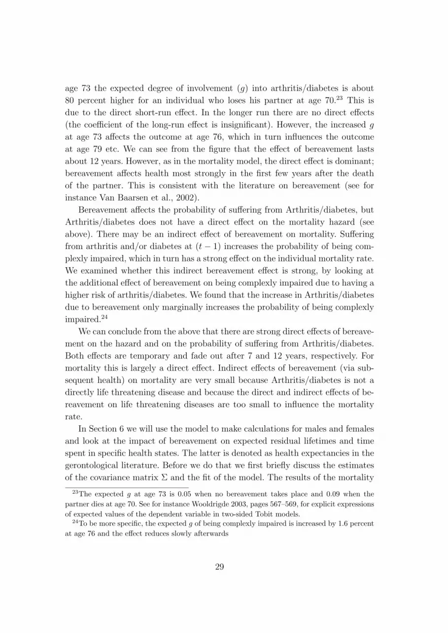
age 73 the expected degree of involvement (g) into arthritis/diabetes is about
80 percent higher for an individual who loses his partner at age 70.23 This is
due to the direct short-run effect. In the longer run there are no direct effects
(the coefficient of the long-run effect is insignificant). However, the increased g
at age 73 affects the outcome at age 76, which in turn influences the outcome
at age 79 etc. We can see from the figure that the effect of bereavement lasts
about 12 years. However, as in the mortality model, the direct effect is dominant;
bereavement affects health most strongly in the first few years after the death
of the partner. This is consistent with the literature on bereavement (see for
instance Van Baarsen et al., 2002).
Bereavement affects the probability of suffering from Arthritis/diabetes, but
Arthritis/diabetes does not have a direct effect on the mortality hazard (see
above). There may be an indirect effect of bereavement on mortality. Suffering
from arthritis and/or diabetes at (t − 1) increases the probability of being com-
plexly impaired, which in turn has a strong effect on the individual mortality rate.
We examined whether this indirect bereavement effect is strong, by looking at
the additional effect of bereavement on being complexly impaired due to having a
higher risk of arthritis/diabetes. We found that the increase in Arthritis/diabetes
due to bereavement only marginally increases the probability of being complexly
impaired.24
We can conclude from the above that there are strong direct effects of bereave-
ment on the hazard and on the probability of suffering from Arthritis/diabetes.
Both effects are temporary and fade out after 7 and 12 years, respectively. For
mortality this is largely a direct effect. Indirect effects of bereavement (via sub-
sequent health) on mortality are very small because Arthritis/diabetes is not a
directly life threatening disease and because the direct and indirect effects of be-
reavement on life threatening diseases are too small to influence the mortality
rate.
In Section 6 we will use the model to make calculations for males and females
and look at the impact of bereavement on expected residual lifetimes and time
spent in specific health states. The latter is denoted as health expectancies in the
gerontological literature. Before we do that we first briefly discuss the estimates
of the covariance matrix Σ and the fit of the model. The results of the mortality
23The expected g at age 73 is 0.05 when no bereavement takes place and 0.09 when the
partner dies at age 70. See for instance Wooldrigde 2003, pages 567–569, for explicit expressions
of expected values of the dependent variable in two-sided Tobit models.24To be more specific, the expected g of being complexly impaired is increased by 1.6 percent
at age 76 and the effect reduces slowly afterwards
29

equation of the spouse as well as the results of the initial conditions are reported
in Appendix B. We do not comment on these results. These models are purely
reduced form and it is therefore difficult to give a meaningful interpretation to
the parameter estimates of these models.
Figure 4 displays the results of the covariance matrix Σ of the unobserved
individual effects. A majority of the variances and covariances of the individual
unobserved effects are not significant.25 This seems to indicate that it is not
necessary to estimate the mortality equation jointly with the health evolution
equations. We performed a Wald test on the joint significance of the parameters
of the matrix Σ. The Wald test rejects the null hypothesis of no correlation
between (αh, αs, ζ2, ζ3, ζ4, ζ5, ν2). Similarly, we perform a series of Wald tests for
the joint significance of the variances and covariances of : (1) the head and spouse
mortality equations, (2) the head mortality equation and (each of) the health
equations, (3) the spouse mortality equation and (each of) the health equations,
and (4) the health equations. The Wald tests indicate that the null hypothesis
of no correlation between unobserved determinants of head and spouse mortality
could not be rejected whereas the other null hypotheses of no correlation between
unobserved determinants of head mortality and health evolution, between spouse
mortality and health evolution, and between the health equations are rejected.
This indicates that the shared risks of mortality between husband and wife go
through unobserved characteristics that influence health status. Our conclusion
from all these tests is that the mortality equations and the health equations
should be jointly estimated.
We have performed an informal check of the fit of our health evolution model.
Figure 9 of Appendix D is based on histograms of the average actual and es-
timated probabilities that a grade of membership g∗kt falls in a specific interval.
The estimated probabilities are calculated using parameters estimates of Model I.
The dotted line connects the tops of the histogram of actual probabilities whereas
the solid line connects the tops of the histogram of the estimated probabilities.
A comparison of the graphs per health dimension indicates that the dynamic
health model fits the observed data quite well. A check on the model fit of the
bivariate mortality model is less straightforward.26 However, we have modelled
the lifetimes with a flexible piecewise constant baseline hazard, time-varying re-
gressors and unobserved characteristics. Generally, it is believed that this is the
25The covariances in Model II (the static model) are strongly significant. The results are
available upon request.26We have stock sampled lifetimes, which makes it difficult to calculate (modified) Kaplan-
Meier estimates that are comparable to the hazard rate predictions of the model.
30
most flexible specification within the class of MPH models. Finally, the results
of Model I may depend on the specification of the initial conditions. To check on
this, we compare the results of the survival models and of the health model in the
static and dynamic specifications. The results are highly comparable, which indi-
cates that our results are not sensitive to the treatment of the initial conditions
problem in our model.
6 Life and health expectancies
Residual life expectancy and time spend in specific health states (called “health
expectancies”) are relevant for health care policy and frequently calculated in the
demographic and gerontological literature. With our model we can differentiate
these with respect to marital status and calculate the fraction of lifetime lost as
well as the increase in health disorders resulting from bereavement.
6.1 Residual life expectancies
Expected residual lifetimes at age s are computed as (see, for instance, Lancaster
1990):
E(s) =
∫ ∞
sS(t) dt
S(s)
We compute the survivor function, S(.) from the estimated model, for each sam-
ple respondent. Subsequently, we average the survivor functions per gender and
within specific age intervals. The expected residual lifetimes E(s) are calculated
per gender and marital status. We do the calculations at the sample average
of the socioeconomic characteristics and health status. We report the results in
Tables 3a and 3b.
Males and females lose 7.6 % (= 2.4 years of life) and 8.3 % (= 2.9 years of
life) respectively of their residual life expectancy after bereavement at age 55-
65. For bereavement at age 65-75, these percentages equal 11 and 12.1 and for
bereavement at age 75-85, 16.0 and 17.3. So the loss of the spouse is found to
significantly decrease the residual lifetimes of both genders and at all ages. Tables
3a and 3b also show that most of the effect arises in the first years of bereavement,
during which the residual life expectancies are largely affected. Afterwards, the
decline in remaining years of life are comparable for (still) married and widowed
individuals. This is in line with what we concluded in the previous section. The
31

Table 3a: Residual life expectancies for males (in years).Age Married Widowed
at age 55-65 at age 65-75 at age 75-85
Number of cases 958 3 31 49
55 31.5 29.1
62 24.6 22.3
66 20.7 18.4 18.4
70 16.7 14.5 14.6
74 13 10.8 11 11.2
78 9.5 7.7 7.9 8.1
81 6.4 5.4 5.6 5.8
85 3.6 3.0 3.2 3.4
Table 3b: Residual life expectancies for females (in years).Age Married Widowed
at age 55-65 at age 65-75 at age 75-85
Number of cases 530 29 84 73
55 34.9 32.0
62 27.9 25.0
66 23.9 21.1 21.1
70 20 17.2 17.2
74 16.2 13.4 13.6 13.8
78 12.5 9.9 10.1 10.3
81 8.9 7.1 7.3 7.5
85 5.5 4.9 5.1 5.3
32

table also shows that widowhood at younger ages affects the remaining life ex-
pectancies the most. At all ages residual life expectancy after the death of the
partner is lower for those who lose their spouse at a relatively young age (55-65)
as compared to those who lose their partner at older ages (65-75 and 75-85).
The residual lifetimes based on our model exceed the numbers provided by
Statistics Netherlands. Our sample concerns a group of married older persons and
their characteristics differ from the characteristics of entire Dutch population. We
report on this in Appendix E.
6.2 Health expectancies
Usually, the calculation of health expectancies involves the use of data on the
prevalence of unhealthy states and mortality. Information on the prevalence of
health states can be obtained from census of survey data and usually one uses
life table information to calculate mortality rates. The average number of years
spend in a health state x onwards from a given age s is then derived from (see
e.g. Sullivan, 1971):
HE(s, x) =
∫ ∞
s
∫xh(t, u)S(t) du dt
S(s)
where h(u, t) assigns weights to health states at age t.
Our approach differs from the the traditional “Sullivan method” in two ways.
First, we base our calculations of residual lifetimes in specific health states on
estimates of a joint model for health and mortality. Second, we do not use census
data on the prevalence of unhealthy states in older population, but use instead the
Grade of Membership and the estimates from our model. Our approach allows
for more detail in the calculation of the health expectancies. We calculate the
average grades of membership per age, gender, and marital status as weights
(h(t, k)=gkt) and use these to dis-aggregate the residual life expectancies27
“Healthy life expectancy” or “active life expectancy” is a particular form of
life expectancy that refers to the expected time spent in health states that are free
from serious disability. “Healthy” health states for older population are generally
associated with the absence of functional limitations. In our analyses, “healthy
life expectancies” are given by HE(s, 1), the number of years remaining in the
27Manton and Stallard (1991) also give estimates of health expectancies of the American older
population using the GoM method. However, their method differs from ours. They first identify
the different health dimensions from a cross section of a survey using the Grade of Membership
method and use Census Data to derive life expectancies E(s) for specific age-gender groups. we
use our model for this. They next combine both elements to derive health expectancies.
33

healthy first dimension. Estimates of residual health expectancies per marital
status at age 70 and 80 are reported in Figures 7 and 8, for males and females
respectively.
Figures 7 and 8 show that after bereavement the share of healthy residual
years of life decrease for both genders. Bereaved males experience a worsening of
health status as (relatively) healthy years – in dimension 1 (healthy) and 2 (other
chronic diseases) – are replaced by unhealthy years – in dimension 4 (serious
arthritis and diabetes) and 5 (complexly impaired). Males lose on average 8.5 %
of their remaining healthy years as a consequence of widowhood. Similar effects
are observed for younger (70 year old) females. So, the calculations show that
after bereavement people spend a larger share of their remaining life suffering
from (serious) chronic diseases In absolute terms, however, bereavement reduces
time spend in unhealthy states. This is caused by the strong direct effect of
bereavement on mortality. The reduction in life years due to bereavement are
stronger than the effects of bereavement on health.
7 Conclusions
This study assesses the effects of spousal bereavement on health and mortality
risks at advanced ages. For that purpose, we specify a bivariate survival model
for husband and wife and a dynamic health evolution model and estimate it on a
rich longitudinal survey. Our approach adds to the literature because we combine
a number of relevant aspects. The mortality hazard of the head respondent allows
for a direct effect of the death of the partner and a range of health indicators.
The health indicators give an accurate description of all dimensions of individual
health and are derived from a broader set of health indicators using a flexible,
non-parametric, data reduction method called the Grade of Membership method.
Health is treated as an endogenous regressor and the dynamic model for health
also allows for a direct effect of spousal bereavement and indirect effect via lagged
health.
We find much higher mortality hazards for individuals with cardiovascular
diseases and complexly impaired individuals. The death of the partner signifi-
cantly increases the mortality rate of the survivor. The effect is strong during the
first three years and disappears after approximately seven years.
With respect to health, we find strong effects of lagged health, indicating on
average aggravation of health disorders. Also the prevalence of one disease in-
creases the risk of getting other diseases in the future. So initially not directly
life threatening diseases (like arthritis or diabetes) increase the risk of obtain-
34

Figure 7: Health expectancies for older males
Married male aged 70, Total life expectancy = 16.7 years
Arthritis13%
Others18%
Complexly impaired
20%
Cardiovascular
diseases23%
Healthy26%
Widowed male aged 70, Total life expectancy = 14.5 years
Arthritis27%
Others8%
Complexly impaired
20%
Cardiovascular
diseases21%
Healthy24%
Married male aged 80, Total life expectancy = 7.5 years
Arthritis13%
Others16%
Complexly impaired
27%
Cardiovascular
diseases27%
Healthy17%
Widowed male aged 80, Total life expectancy = 6.6 years
Arthritis22%
Others11%
Complexly impaired
30%
Cardiovascular
diseases22%
Healthy15%
35

Figure 8: Health expectancies for older females
Married female aged 70, Total life expectancy = 20.0 years
Arthritis29%
Others22%
Complexly impaired
18%
Cardiovascular
diseases11%
Healthy20%
Widowed female aged 70, Total life expectancy = 17.2 years
Arthritis31%
Others21%
Complexly impaired
23%
Cardiovascular
diseases10%
Healthy15%
Married female aged 80, Total life expectancy = 10.0 years
Arthritis30%
Others17%
Complexly impaired
27%
Cardiovascular
diseases16% Healthy
10%
Widowed female aged 80, Total life expectancy = 8.3 years
Arthritis29%
Others20%
Complexly impaired
26%
Cardiovascular
diseases16% Healthy
9%
36

ing life threatening diseases later in life and therefore later life mortality. The
death of the partner significantly increases the probability of suffering from arthri-
tis/diabetes. This effect is not permanent, but can last up to 12 years. However,
as in the mortality model, the direct effects of bereavement are stronger than the
longer run effects; bereavement affects the probability of arthritis/diabetes most
strongly in the first few years just after the death of the partner. We find no
direct effects of bereavement on other health disorders. Also indirect effects (via
arthritis/diabetes) of bereavement on other health disorders are small.
We used the model to calculate residual life and health expectancies differen-
tiated per marital status. We find that males and females lose on average 11.5 %
and 12.5 % respectively of their residual life expectancy after bereavement. Most
of the effect takes place in the first years of bereavement. We also calculated
health expectancies, i.e. residual life time spend in specific health states. We find
that bereavement affects the share of healthy years in residual lifetime, primarily
because healthy years are replaced by years of having serious arthritis and dia-
betes and of being complexly impaired. In absolute terms, however, bereavement
reduces time spent in unhealthy states. This is caused by the strong direct effect
of bereavement on mortality. The reduction in life years due to bereavement are
stronger than the effects of bereavement on health.
The strong direct effects of bereavement are important for policies aimed at
the elderly. It suggests that monitoring and/or interventions just after spousal
bereavement are important for the length of remaining life and for the physical
and mental health-related quality of life of older bereaved persons.
37
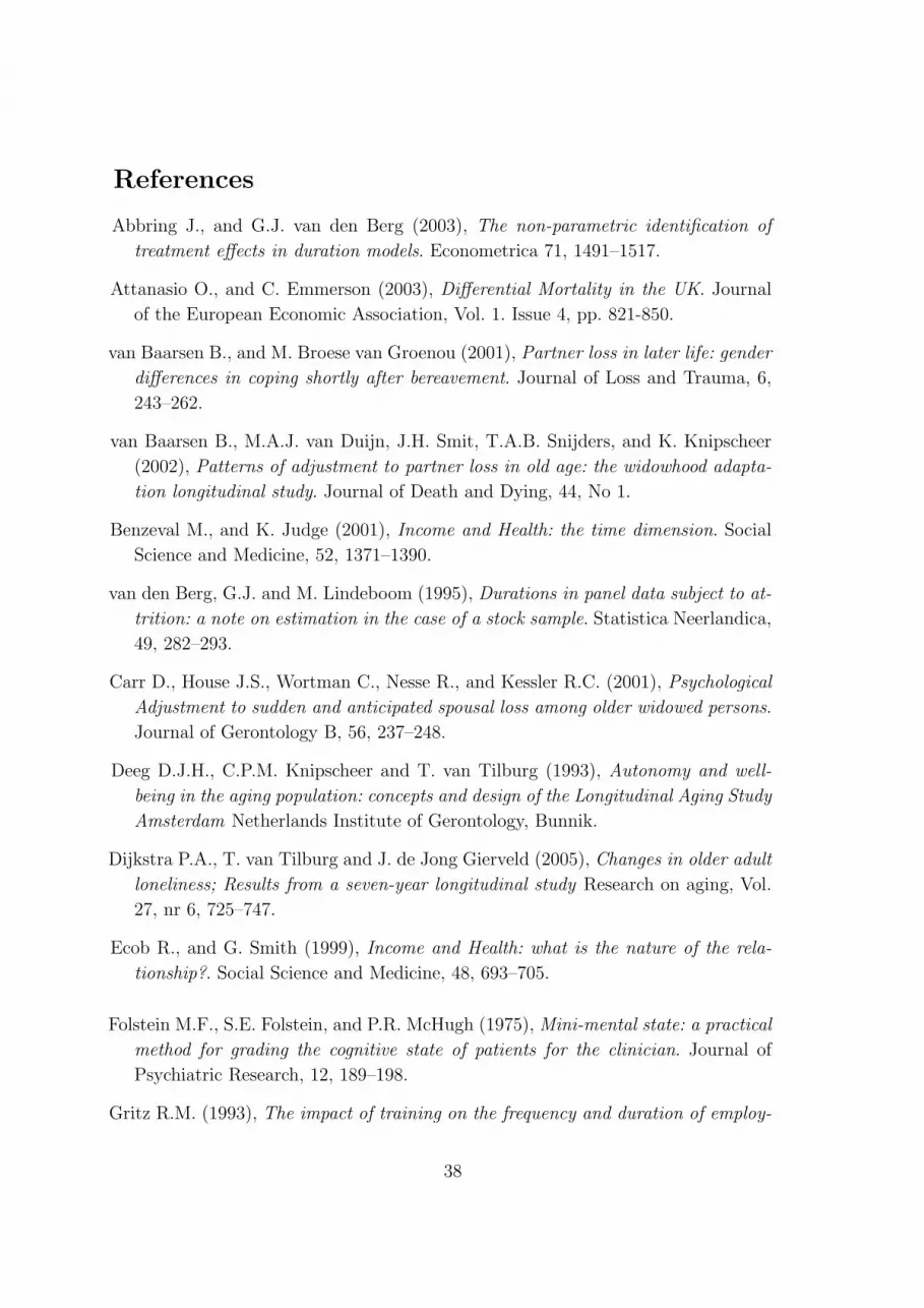
References
Abbring J., and G.J. van den Berg (2003), The non-parametric identification of
treatment effects in duration models. Econometrica 71, 1491–1517.
Attanasio O., and C. Emmerson (2003), Differential Mortality in the UK. Journal
of the European Economic Association, Vol. 1. Issue 4, pp. 821-850.
van Baarsen B., and M. Broese van Groenou (2001), Partner loss in later life: gender
differences in coping shortly after bereavement. Journal of Loss and Trauma, 6,
243–262.
van Baarsen B., M.A.J. van Duijn, J.H. Smit, T.A.B. Snijders, and K. Knipscheer
(2002), Patterns of adjustment to partner loss in old age: the widowhood adapta-
tion longitudinal study. Journal of Death and Dying, 44, No 1.
Benzeval M., and K. Judge (2001), Income and Health: the time dimension. Social
Science and Medicine, 52, 1371–1390.
van den Berg, G.J. and M. Lindeboom (1995), Durations in panel data subject to at-
trition: a note on estimation in the case of a stock sample. Statistica Neerlandica,
49, 282–293.
Carr D., House J.S., Wortman C., Nesse R., and Kessler R.C. (2001), Psychological
Adjustment to sudden and anticipated spousal loss among older widowed persons.
Journal of Gerontology B, 56, 237–248.
Deeg D.J.H., C.P.M. Knipscheer and T. van Tilburg (1993), Autonomy and well-
being in the aging population: concepts and design of the Longitudinal Aging Study
Amsterdam Netherlands Institute of Gerontology, Bunnik.
Dijkstra P.A., T. van Tilburg and J. de Jong Gierveld (2005), Changes in older adult
loneliness; Results from a seven-year longitudinal study Research on aging, Vol.
27, nr 6, 725–747.
Ecob R., and G. Smith (1999), Income and Health: what is the nature of the rela-
tionship?. Social Science and Medicine, 48, 693–705.
Folstein M.F., S.E. Folstein, and P.R. McHugh (1975), Mini-mental state: a practical
method for grading the cognitive state of patients for the clinician. Journal of
Psychiatric Research, 12, 189–198.
Gritz R.M. (1993), The impact of training on the frequency and duration of employ-
38

ment. Journal of Econometrics, 57, 21–51.
Gulranik J.M. (1994), A short physical performance battery assessing lower extremity
function: association with self-reported disability and prediction of mortality and
nursing home admission. Journal of Gerontology B, 49, 85–94.
Heckman J.J., C. Manski, and D. McFadden (1981), The Incidental Parameters
Problem and the Problem of Initial Conditions in Estimating A Discrete Time-
Discrete Data Stochastic Process and Some Monte Carlo Evidence. Structural
Analysis of Discrete Data With Econometric Applications. M.I.T. Press.
Irwin M., M. Daniels, and H. Weiner (1987), Immune and neuroendocrine changes
during bereavement. Psychiatric Clinics of North America, 10, 449–465.
Irwin M. and J. Pike (1993), Bereavement, depressive symptoms, and immune func-
tion. In Handbook of Bereavement. Theory, Research, and Intervention, ed. M.
Stroebe, W. Stroebe, R.O. Hansson, 160–171. New York: Cambridge University
Press.
Klein J.P. (1992), Semiparametric Examination of Random Effects Using the Cox
Model Based on the EM Algorithm. Biometrics, 48, 795–806.
Koehn S. (2001), Food for Life/Back to the Table. Report of research findings.
Lakdawalla D.N. and T. Philipson (2002), The rise in old-age longevity and the
market for long-term care. American Economic Review 92(1) 295-306.
Lancaster T. (1990), The Econometric Analysis of Transition Data. Cambridge Uni-
versity Press.
Lichtenstein P., M. Gatz, and S. Berg (1998), A twin study of mortality after spousal
bereavement. Psychological Medicine, 28, 635–643.
Lillard, L.A. and C.W.A. Panis (1996), Marital status and mortality: the role of
health, Demography, 33, 313–327.
Manton K., and E. Stallard (1991), Cross-sectional estimates of active life expectancy
for the U.S. elderly and oldest-old populations. Journal of Gerontology B, 46,
170–182.
Manton K., M. Woodbury, E. Stallard, and L. Corder (1992), The use of Grade of
Membership techniques to estimate regression relationships. Sociological Method-
ology, 22, 150–182.
39
McGarry K. and R.F. Schoeni (2005), Widow(er) poverty and out-of-pocket medical
expenditures at the end of life. Journals of Gerontology B, 60, S160–S168.
Nathan, D.M. (1993), Long-term complications of diabetes mellitus. New England
Journal of Medicine, 328, 1676–1685.
Norton E. (2000), Long-term care. Handbooks of Health Economics, Chapter 21.
Osterweis, M., F. Solomon and M. Green (1984), Bereavement: reactions, conse-
quences and care. National Academies Press, Washington DC.
Portrait F. (2000), Long-term care services for the Dutch elderly – An investigation
into the process of utilization. PhD thesis, Vrije Universiteit, Amsterdam.
Prigerson H., A.J. Bierhals, S.V. Kasl, C.F. Reynolds, M.K. Shear, N. Day, L.C.
Beery, J.T. Newsom, and S. Jacobs (1997), Traumatic grief as a risk factor for
mental and physical morbidity. American Journal of Psychiatry, 154, 616–623.
Prigerson H., P. Maciejewski, and R. Rosenheck (2000), Preliminary explorations
of the harmful interactive effects of widowhood and marital harmony on health,
health service use, and health service costs. The Gerontologist, 40, 349–357.
Radloff, L.S. (1977), The CES-D scale: a self-report depression scale for research in
the general population, Applied Psychological Measurement, 1, 385–401.
Robine J., C. Jagger, and Mathers C. (2003), Determining health expectancies, John
Wiley and sons, Ltd.
Sixma H., and Ultee, W.C. (1983), Een Beroepsprestigeschaal voor Nederland in de
Jaren Tachtig (in English: Occupational prestige score for the Netherlands in the
eighties). Mens en Maatschappij, 58, 360–382.
van Sonsbeek, J.L.A. (1988), Methodological and substantial aspects of the OECD
indicator of chronic functional limitations. Maandbericht Gezondheid (Central
Bureau of Statistics), Holland.
Stern S. (1997), Simulation-Based Estimation Journal of Economic Literature, XXXV,
2006–2039.
Sullivan D. (1971), A single index of mortality and morbidity, HSMHA report, 86.
van Tilburg, T., P. Dijkstra, A. Liefbroer, and M. Broese van Groenou (1992),
Sourcebook of Living Arrangements and Social Networks of Older Adults in the
Netherlands. Vrije Universiteit Amsterdam.
40

Williams, K. (2004), The transition to widowhood and the social regulation of health:
consequences for health and health risk behavior, Journal of Gerontology B, 59,
343–349.
Woodbury M.A., and J. Clive (1974), Clinical Pure Types as a Fuzzy Partition.
Journal of Cybernetics, 4, 111–121.
Woodbury M.A., J. Clive, and A. Garson (1978), Mathematical Typology: A Grade of
Membership Technique for Obtaining Disease Definition. Computers and Biomed-
ical Research, 11, 277–298.
Woodbury, M.A. and K.G. Manton (1982), A new procedure for analysis of medical
classification. Methods of Information in Medicine, 21, 209–220.
Wooldridge J.M. (2003), Introductory econometrics: a modern approach. Thomson
South-Western.
41

Appendix A
Table A1: GoM Parameters λkjl, wave I
Score Freq. K=1 K=2 K=3 K=4 K=5
Self-reported test 0 0.591 1 0.612 0.358 0.367 0.433
on mobility 1 0.191 0 0.246 0.516 0.289 0.086
2 0.115 0 0.142 0.126 0.344 0.047
3 0.103 0 0 0 0 0.434
Performance test 0 0.545 0.642 0.600 0.481 0.565 0.285
(cardigan) 1 0.435 0.358 0.400 0.519 0.435 0.643
2 0.020 0 0 0 0 0.072
MMSE ≥ 23 0.900 1 1 1 1 0.604
< 23 0.100 0 0 0 0 0.396
CES-D ≤ 16 0.855 1 0.847 0.851 0.849 0.732
> 16 0.145 0 0.153 0.149 0.151 0.268
Vision Good 0.885 1 0.864 0.874 0.910 0.786
Bad 0.115 0 0.136 0.126 0.090 0.214
Hearing Good 0.940 1 1 1 1 0.770
Bad 0.060 0 0 0 0 0.230
COPD N 0.884 1 1 1 1 0.540
Y 0.116 0 0 0 0 0.460
Medical treatment N 0.915 1 1 1 1 0.672
(COPD) Y 0.085 0 0 0 0 0.328
Heart diseases N 0.804 1 1 0 1 1
Y 0.196 0 0 1 0 0
Medical treatment N 0.826 1 1 0.111 1 1
(Heart diseases) Y 0.174 0 0 0.889 0 0
Atherosclerosis N 0.902 1 1 0.591 1 1
Y 0.098 0 0 0.409 0 0
Medical treatment N 0.930 1 1 0.712 1 1
(Atherosclerosis) Y 0.070 0 0 0.288 0 0
Diabetes N 0.922 1 1 1 0.693 1
Y 0.078 0 0 0 0.307 0
Medical treatment N 0.926 1 1 1 0.709 1
(Diabetes) Y 0.074 0 0 0 0.291 0
Stroke N 0.944 1 1 1 1 0.780
Y 0.056 0 0 0 0 0.220
Medical treatment N 0.958 1 1 1 1 0.842
(Stroke) Y 0.042 0 0 0 0 0.158
Arthritis N 0.651 1 0.700 0.825 0 0.689
Y 0.349 0 0.300 0.175 1 0.311
Medical treatment N 0.850 1 1 1 0.336 1
(Arthritis) Y 0.150 0 0 0 0.664 0
Cancer N 0.907 1 1 1 1 0.650
Y 0.093 0 0 0 0 0.350
Medical treatment N 0.939 1 1 1 1 0.775
(Cancer) Y 0.061 0 0 0 0 0.225
Other chronic diseases N 0.667 1 0 0.966 1 0.887
Y 0.333 0 1 0.034 0 0.113
Medical treatment N 0.767 1 0 1 1 1
(Other chronic diseases) Y 0.233 0 1 0 0 0
The third column of Table A1 reports sample proportions of various health dis-
orders. The characteristics of the different health dimensions are determined by
examination of the K profile probabilities λkjl and their comparison to the sample
proportions of interest.
42

Appendix B
Table 2b: Results of Model I (second part): mortality of spouse and initial conditions
Variables Coeff. t-value Variables Coeff. t-value
Mortality of spouses Baseline hazard for spouses
Female -0.890 -6.91 γ1 (32/70) 0.008 3.32
Education -0.110 -3.48 γ2 (70/74) 0.028 3.19
Occupational level 0.020 0.38 γ3 (74/78) 0.072 3.28
Urbanization -0.038 -1.94 γ4 (78/82) 0.207 3.25
Church attendance -0.044 -1.40 γ5 (82/86) 0.406 3.15
γ6 (86/95) 0.424 2.74
Health equation (Initial conditions)
Other chronic diseases Cardiovascular diseases
Constant -1.129 -4.16 Constant -0.321 -1.57
Age 0.491 0.65 Age 1.358 2.29
Age2 -0.647 -0.69 Age2 -0.539 -0.76
Female 0.696 3.63 Female -0.810 -5.48
Education 0.172 0.81 Education -0.229 -1.46
Urbanization -0.102 -0.67 Urbanization 0.061 0.53
Church attendance 0.018 0.15 Church attendance -0.076 -0.80
σ1 1.643 8.18 σ2 0.890 9.11
Arthritis/Diabetes Complexly impaired
Constant -0.965 -5.84 Constant -0.353 -2.85
Age 0.816 1.84 Age 0.899 2.47
Age2 -0.387 -0.72 Age2 -0.001 -0.00
Female 0.645 5.59 Female 0.008 0.09
Education -0.266 -2.12 Education -0.335 -3.39
Urbanization -0.040 -0.44 Urbanization 0.024 0.33
Church attendance 0.028 0.38 Church attendance -0.246 -3.86
σ3 0.239 16.830 σ4 0.166 16.74
One-factor error specification
l2 -0.133 -0.64
l3 0.205 0.62
l4 -1.630 -2.20
43

Appendix C
Table 2c: Model 2: Mortality of head and spouse and a static health model of the head
Variables Coeff. t-value Variables (Age classes) Coeff. t-value
Mortality of LASA respondents Baseline hazard for LASA respondents
Female -0.482 -4.50 γ1 (55/62) 0.005 2.74
Education 0.018 0.77 γ2 (62/66) 0.010 3.08
Income -1.057 -4.87 γ3 (66/70) 0.016 3.29
Urbanization 0.026 1.76 γ4 (70/74) 0.030 3.57
Church attendance -0.112 -4.62 γ5 (74/78) 0.063 3.72
TSB (short run) -0.330 -1.38 γ6 (78/82) 0.121 3.80
Quadratic TSB (short run) 0.319 4.76 γ7 (82/85) 0.303 3.81
TSB (long run) 0.797 3.72 γ8 (86/92) 0.454 3.45
Quadratic TSB (long run) -0.130 -2.61
Dummy refusals -1.358 -10.78
Other Chronic diseases 0.444 2.40
Cardiovascular diseases 0.650 3.74
Arthritis/Diabetes -0.043 -0.21
Complexly impaired 1.275 7.23
Mortality of spouses Baseline hazard for spouses
Female -0.984 -8.15 γ1 (32/70) 0.017 3.47
Education -0.110 -3.81 γ2 (70/74) 0.051 3.36
Occupational level 0.033 0.70 γ3 (74/78) 0.110 3.41
Urbanization -0.040 -2.17 γ4 (78/82) 0.265 3.42
Church attendance -0.059 -2.03 γ5 (82/86) 0.478 3.39
γ6 (86/95) 0.547 3.00
Health model
Other Chronic diseases Cardiovascular diseases
Constant -0.860 -6.24 Constant -0.141 -1.79
Age -0.057 -0.15 Age 1.199 5.11
Age2 -0.069 -0.16 Age2 -0.542 -2.17
Female 0.516 5.72 Female -0.647 -13.70
Education 0.172 1.49 Education -0.130 -2.17
Income -0.016 -0.14 Income -0.137 -2.93
Church attendance -0.045 -0.76 Church attendance -0.122 -3.83
Urbanization -0.177 -2.40 Urbanization 0.010 0.27
TSB (short run) 0.008 0.16 TSB (short run) -0.002 -0.02
TSB (long run) 0.019 0.80 TSB (long run) -0.061 -1.44
σ1 1.305 14.14 σ2 0.425 19.80
Arthritis/Diabetes Complexly impaired
Constant -0.933 -12.75 Constant -0.218 -3.77
Age 0.972 4.91 Age 0.957 5.63
Age2 -0.603 -2.83 Age2 -0.118 -0.65
Female 0.643 13.98 Female -0.050 -1.40
Education -0.049 -0.86 Education -0.238 -5.17
Income -0.137 -2.50 Income -0.137 -2.93
Urbanization 0.031 0.87 Urbanization -0.024 -0.82
Church attendance 0.081 2.82 Church attendance -0.104 -4.08
TSB (short run) 0.094 2.31 TSB (short run) -0.002 -0.08
TSB (long run) 0.036 1.74 TSB (long run) 0.006 0.37
σ3 0.379 22.22 σ4 0.263 20.94
Note: TSB = Time since bereavement
44

Appendix D
Figure 9: Informal check dynamic health model
0
0 .1
0 .2
0 .3
0 .4
0 .5
0 .6
0 .7
0 0 .1 0 .2 0 .3 0 .4 0 .5 0 .6 0 .7 0 .8 0 .9 1
O the r d ise ase s
Freq
uenc
y
: Realized Values: Predicted Values
0
0 .1
0 .2
0 .3
0 .4
0 .5
0 .6
0 .7
0 0 .1 0 .2 0 .3 0 .4 0 .5 0 .6 0 .7 0 .8 0 .9 1
C a rd iovascu lar d ise ase s
Freq
uenc
y
0
0 .1
0 .2
0 .3
0 .4
0 .5
0 .6
0 .7
0 0 .1 0 .2 0 .3 0 .4 0 .5 0 .6 0 .7 0 .8 0 .9 1
A r th r itis
Freq
uenc
y
0
0 .1
0 .2
0 .3
0 .4
0 .5
0 .6
0 .7
0 0 .1 0 .2 0 .3 0 .4 0 .5 0 .6 0 .7 0 .8 0 .9 1
O the r d ise ase s
Freq
uenc
y
45

Appendix E
Figure 10: Sample and Statistics-Netherlands hazard rates
0
0.02
0.04
0.06
0.08
0.1
0.12
0.14
55 64 73 81Age
Haz
ard r
ates
(w
ithi
n th
ree
yea
rs o
f ag
e)
Female (Sample)Female (Statistics Netherlands)Male (Sample)Male (Statistics Netherlands)
Statistics Netherlands calculate “average residual life expectancies” – i.e. residual
lifetimes for individuals with average health status, socioeconomic characteristics
and marital status. Our sample is not representative of the Dutch older population
as we selected married individuals at baseline. Figure 10 shows hazard rate from
our model (estimated on the sample of married individuals) and hazard rates from
the Statistics Netherlands. It is clear that our model estimates are lower than
the estimates from Statistics Netherlands. We further compared the averages of
the explanatory variables of our (married) sample with the population averages.
On average, the sample respondents are younger, higher educated, have higher
incomes, and go more often to church. These factors are found to be associated
(in our model and in the literature) with lower mortality and morbidity.
46
Top Related
Copyright © 2022 FDOKUMEN

