MARINE ECOLOGY PROGRESS SERIESMar Ecol Prog Ser

Vol. 382: 297–311, 2009doi: 10.3354/meps08030

Published April 30

INTRODUCTION

The European Water Framework Directive (WFD)establishes a basis for the protection of ground, conti-nental, transitional and coastal waters. It aims atachieving a good ecological status (ES) for all Euro-pean water bodies by 2015. The first step consists ofassessing the current ES of these water bodies, which

is based on a large variety of hydromorphological,physicochemical and biological parameters. In order tounravel natural and man-induced changes, ES valuesare derived from ecological quality ratios (EQR), whichcorrespond to the ratio of the value of the consideredparameter at each sampled station divided by thevalue of the same parameter at a reference (i.e. non-impacted) station (Wallin et al. 2003).

© Inter-Research 2009 · www.int-res.com*Email: a.gremare@epoc.u-bordeaux1.fr

Addresses for other authors are given in the Electronic Appen-dix at www.int-res.com/articles/suppl/m382p221_app.pdf

Comparison of the performances of two bioticindices based on the MacroBen database

A. Grémare1,*, C. Labrune, E. Vanden Berghe, J. M. Amouroux, G. Bachelet,M. L. Zettler, J. Vanaverbeke, D. Fleischer, L. Bigot, O. Maire, B. Deflandre,

J. Craeymeersch, S. Degraer, C. Dounas, G. Duineveld, C. Heip, M. Herrmann,H. Hummel, I. Karakassis, M. Kedra, M. Kendall, P. Kingston, J. Laudien,

A. Occhipinti-Ambrogi, E. Rachor, R. Sardá, J. Speybroeck, G. Van Hoey, M. Vincx,P. Whomersley, W. Willems, M. W8odarska-Kowalczuk, A. Zenetose

1Université Bordeaux 1, CNRS, UMR 5805 EPOC, Station Marine d’Arcachon, 2 rue du Professeur Jolyet,33120 Arcachon, France

ABSTRACT: The pan-European MacroBen database was used to compare the AZTI Marine BioticIndex (AMBI) and the Benthic Quality Index (BQIES), 2 biotic indices which rely on 2 distinct assess-ments of species sensitivity/tolerance (i.e. AMBI EG and BQI E[S50]0.05) and which up to now haveonly been compared on restricted data sets. A total of 12 409 stations were selected from the data-base. This subset (indicator database) was later divided into 4 marine and 1 estuarine subareas. Wecomputed E(S50)0.05 in 643 taxa, which accounted for 91.8% of the total abundances in the wholemarine indicator database. AMBI EG and E(S50)0.05 correlated poorly. Marked heterogeneities inE(S50)0.05 between the marine and estuarine North Sea and between the 4 marine subareas suggestthat sensitivity/tolerance levels vary among geographical areas. High values of AMBI were alwaysassociated with low values of BQIES, which underlines the coherence of these 2 indices in identifyingstations with a bad ecological status (ES). Conversely, low values of AMBI were sometimes associatedwith low values of BQIES resulting in the attribution of a good ES by AMBI and a bad ES by BQIES.This was caused by the dominance of species classified as sensitive by AMBI and tolerant by BQIES.Some of these species are known to be sensitive to natural disturbance, which highlights the ten-dency of BQIES to automatically classify dominant species as tolerant. Both indices thus present weak-nesses in their way of assessing sensitivity/tolerance levels (i.e. existence of a single sensitivity/toler-ance list for AMBI and the tight relationship between dominance and tolerance for BQIES). Futurestudies should focus on the (1) clarification of the sensitivity/tolerance levels of the species identifiedas problematic, and (2) assessment of the relationships between AMBI EG and E(S50)0.05 within andbetween combinations of geographical areas and habitats.

KEY WORDS: AZTI Marine Biotic Index · Benthic Quality Index · Macrozoobenthos · Waterframework directive

Resale or republication not permitted without written consent of the publisher

Contribution to the Theme Section ‘Large-scale studies of the European benthos: the MacroBen database’ OPENPEN ACCESSCCESS

Mar Ecol Prog Ser 382: 297–311, 2009

Macrozoobenthos is one of the biological compart-ments considered by the WFD (Borja et al. 2004a, Borja2005) and a large variety of biotic indices use its com-position to infer ES (Grall & Glémarec 1997, Borja et al.2000, Gomez Gesteira & Dauvin 2000, Rosenberg et al.2004). In spite of their diversity, most of these indicesare based on the same paradigm: disturbances aregenerating secondary successions during which toler-ant species are at first dominant and then progres-sively replaced by sensitive species (Pearson & Rosen-berg 1978). There is, thus, more need for testing andunifying the existing benthic biotic indices than forproducing new ones (Diaz et al. 2004). Two of the mainindices introduced in view of the implementation of theWFD are (1) the AZTI Marine Biotic Index (AMBI;Borja et al. 2000), and (2) the Benthic Quality Index(BQI; Rosenberg et al. 2004). Although these 2 indicesrely on the same concept, they differ in (1) their waysof assessing species sensitivity/tolerance levels, (2) theconsideration of species richness, and (3) the proce-dures used to convert computed indices of ES.

In AMBI, sensitivity/tolerance levels are assessedbased on the compilation of expert knowledge and itstranslation into ecological groups (AMBI EG). Thisresults in a single sensitivity/tolerance per species thatis used for all data sets irrespective of geographic loca-tion (Borja et al. 2000, Borja et al. 2003, Salas et al.2004, Muxika et al. 2005). Conversely, for BQI, Rosen-berg et al. (2004) assume that species sensitivity/toler-ance levels vary according to geographical location.The assessment of sensitivity/tolerance within BQI isbased on the concept of E(S50)0.05 (see ‘Data and meth-ods’ for definition) (Rosenberg et al. 2004). The avail-ability of E(S50)0.05 constitutes a severe limitation to thecomputation of BQI, which is either restricted to largedata sets (Rosenberg et al. 2004, Labrune et al. 2006,Dauvin et al. 2007, Zettler et al. 2007) or to areas wherea list of E(S50)0.05 is available (Reiss & Kröncke 2005).

The computation of AMBI is based on the sole sensi-tivity/tolerance concept (Borja et al. 2000), which makesit largely sampling effort-independent (Fleischer et al.2007, Muxika et al. 2007b). Conversely, BQI also takesinto account species richness (S) through a log(S + 1)term (Rosenberg et al. 2004), which makes it samplingeffort-dependent when computed on lumped data(Fleischer et al. 2007) and/or on individual samples col-lected with different gears. This constitutes anotherrestriction to its use since large databases are (1) oftenconstituted of several surveys with different samplingstrategies (see Table 1 for the present study), and (2)often comprised of a significant proportion of lumpeddata (i.e. 96.3% of all stations during the present study).Fleischer et al. (2007) proposed to overcome this diffi-culty by replacing log(S + 1) by log(E[S50] + 1) andproved that the so-modified BQI (i.e. BQIES) is indepen-

dent of sampling effort and correlates tightly with BQI.AMBI uses a single scale to infer ES (Borja et al.

2004a), whereas BQI assumes that for each habitat thestation with the highest BQI constitutes a valid refer-ence for the computation of EQR. The stations with anEQR higher than 0.6 are then considered to at least bein a good ES (Rosenberg et al. 2004).

Multivariate AMBI (M-AMBI) was recently intro-duced as a refinement of AMBI (Borja et al. 2004b,Borja et al. 2007, Muxika et al. 2007a). Its computationinvolves a factorial correspondence analysis (FCA)based on AMBI, species richness and the Shannon-Wiener diversity index, H ’. FCAs are carried out foreach habitat and 2 bad and good reference stations areincluded. The coordinates of the projection of the sta-tions along the axis linking the bad and good referencestations in the first plane of the FCA constitute EQR,which are transformed into ES using an appropriateconversion scale (Wallin et al. 2003). M-AMBI is muchmore similar to BQI than AMBI since it accounts forspecies richness and uses several scales to infer ES.BQI and M-AMBI, however, still largely differ in theirassessments of species sensitivity/tolerance.

Both AMBI and BQI were initially proposed andtested based on individual data sets (Borja et al. 2000,Rosenberg et al. 2004). AMBI has, since then, beentested on a large variety of other (but still mostly indi-vidual) data sets (Borja et al. 2000, 2003, Salas et al.2004, Marin-Guirao et al. 2005, Muniz et al. 2005,Muxika et al. 2005, Bigot et al. 2008, Blanchet et al.2008), BQI has been tested on a much smaller num-ber of datasets due to the difficulty in computingE(S50)0.05. AMBI and BQI have recently been com-pared in the North Sea (Reiss & Kröncke 2005), theGulf of Lions (Labrune et al. 2006), the Seine estuary(Dauvin et al. 2007) and the Baltic Sea (Zettler et al.2007). All comparisons have shown major discrepan-cies but have largely ignored their potential causes.The adequacy of the use of a single sensitivity/toler-ance list by AMBI as opposed to BQI is, for example,yet to be tested partly due to the lack of any com-prehensive database at the pan-European level. TheNetwork of Excellence Marine Biodiversity and Eco-system Functioning (MarBEF) has recently filled thisgap for soft-bottom macrozoobenthos by creating theMacroBen database. The aim of the present study isto use this new tool to (1) promote the use of BQIES byproviding lists of E(S50)0.05 both at the pan-Europeanlevel and within distinct geographic subareas, (2)compare AMBI EG and E(S50)0.05, (3) assess the valid-ity of the use of a single list of sensitivity/tolerancelevels by comparing E(S50)0.05 between subareas, (4)assess the relationships between AMBI and BQIES

and (5) compare the ES assessments derived fromAMBI and BQIES.

298

Grémare et al.: Comparison of two biotic indices

DATA AND METHODS

MacroBen database. The main characteristics ofMacroBen are described in Vanden Berghe et al. (2009,this Theme Section) and will not be repeated here. Thefiltering procedure used during the present study con-sisted of selecting (1) quantitative data, (2) adult animaltaxa, (3) organisms identified to the species level, (4)non-colonial organisms and (5) samples collected after1980. Baltic Sea samples were excluded because an ex-tensive comparison between AMBI and BQI has re-cently been carried out in this area (Zettler et al. 2007),and Black Sea samples were excluded because theywere too few. The data set was further reduced byconsidering only the most recent sampling date foreach station. This reduced indicator database was com-

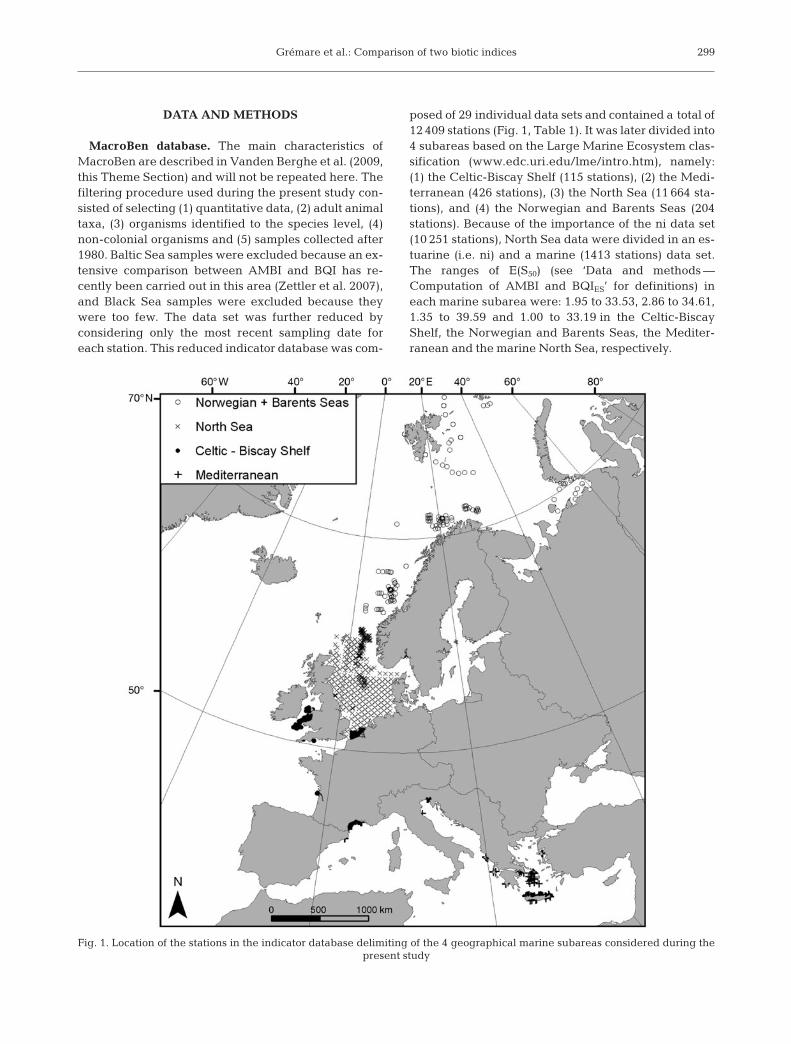
posed of 29 individual data sets and contained a total of12 409 stations (Fig. 1, Table 1). It was later divided into4 subareas based on the Large Marine Ecosystem clas-sification (www.edc.uri.edu/lme/intro.htm), namely:(1) the Celtic-Biscay Shelf (115 stations), (2) the Medi-terranean (426 stations), (3) the North Sea (11 664 sta-tions), and (4) the Norwegian and Barents Seas (204stations). Because of the importance of the ni data set(10 251 stations), North Sea data were divided in an es-tuarine (i.e. ni) and a marine (1413 stations) data set.The ranges of E(S50) (see ‘Data and methods —Computation of AMBI and BQIES’ for definitions) ineach marine subarea were: 1.95 to 33.53, 2.86 to 34.61,1.35 to 39.59 and 1.00 to 33.19 in the Celtic-BiscayShelf, the Norwegian and Barents Seas, the Mediter-ranean and the marine North Sea, respectively.

299

Fig. 1. Location of the stations in the indicator database delimiting of the 4 geographical marine subareas considered during the present study

Mar Ecol Prog Ser 382: 297–311, 2009

Computation of AMBI and BQIES. AMBI was com-puted as:

AMBI = [(0 × %GI) + (1.5 × %GII) + (3 × %GIII) + (4.5 ×%GIV) + (6 × %GV)]/100 (1)

where %GI is the relative abundance of disturbance-sensitive species, %GII is the relative abundance ofdisturbance-indifferent species, %GIII is the relativeabundance of disturbance-tolerant species, %GIV isthe relative abundance of second-order opportunisticspecies and %GV is the relative abundance of first-order opportunistic species (Borja et al. 2000). AMBIwas computed as recommended by Borja & Muxika(2005) using a specific function implemented in Mac-roBen and based on the species reference list availableat www.azti.es in July 2006. We used a single fixedscale to infer ES from AMBI (Borja et al. 2004a).

E(S50)0.05 is defined as the E(S50) (Hurlbert 1971) cor-responding to the 5 lowest percentiles of the total

abundance of the considered species within the stud-ied area (Rosenberg et al. 2004). E(S50)0.05 values werecomputed for the whole marine indicator data set andeach subarea.

BQIES was then computed as:

(2)

where Ai is the abundance of the ith species at the con-sidered station, E(S50)0.05i is the E(S50)0.05 of species i inthe considered subarea, ATot is the total abundance ofthe individuals belonging to the species for whichE(S50)0.05 can be computed and E(S50) is the expectednumber of species in a sample of 50 individuals takenat the considered station (Fleischer et al. 2007).E(S50)0.05 and BQIES were computed on lumped datausing a specific function implemented in MacroBen.E(S50)0.05 values were not computed for species presentat less than 20 stations. We used several conversion

BQI E SESTot

= × ( )⎡⎣⎢

⎤⎦⎥

⎧⎨⎩

⎫⎬⎭

×=

∑ AA

ii

i

s

50 0 051

10. log EE S50 1( ) +[ ]

300

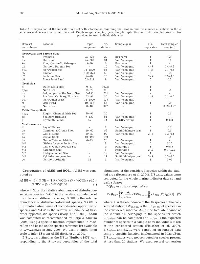
Data set Location Depth No. Sample gear No. Total sampledand subarea range (m) stations replicates area (m2)

Norwegian and Barents Seasar Svalbard 75–335 22 Box corer 1 0.1hs Hornsund 25–203 34 Van Veen grab 1 0.1ko Kongsfjorden/Spitsbergen 5–30 6 Box corer 1 –o2 Northern Barents Sea – 10 Van Veen grab 4–5 0.4–0.5o4NB Norwegian Sea 71–1520 55 Van Veen grab 1–5 0.1–0.5o6 Finmark 160–374 53 Van Veen grab 5 0.5o7 Pechoran Sea 7–207 15 Van Veen grab 3–5 0.3–0.5o8 Franz Josef Land 52–312 9 Van Veen grab 5 0.5

North Seani Dutch Delta area 0–57 10251 – 1 –npNS North Sea 35–70 20 – 1 0.1ns Belgian part of the North Sea 0–150 231 Van Veen grab – –o3 Statfjord, Oseberg, Ekosfisk 65–91 30 Van Veen grab 1–5 0.1–0.5o4NS Norwegian coast 71–1520 128 Van Veen grab – –of Oslo Fjord 19–356 57 Van Veen grab 1 0.1ug North Sea 0–40 947 – 3 0.09–0.27

Celtic-Biscay ShelfnpCS English Channel, Irish Sea 50–96 20 – 1 0.1o5 Southern Irish Sea 7–130 51 Van Veen grab 1 –pl Plymouth Sound 15 44 SCUBA diving 1 0.008

Mediterraneanbl Bay of Blanes – 2 Van Veen grab 5 0.3do Continental Cretan Shelf 10–60 56 Smith McIntyre grab 1 0.1gr Gulf of Lions 10–50 92 Van Veen grab 2–4 0.2–0.4ka Cretan Shelf 10–190 199 – – 0.1lm Gulf of Trieste, Adriatic 4–25 28 Van Veen grab 1 –M0 Gialova Lagoon, Ionian Sea – 7 Van Veen grab 5 0.25M2 Gulf of Geras, Aegean Sea – 9 Ponar grab 1 0.045M3 Saronikos Gulf – 6 Ponar grab 2–5 0.1–0.25M7 Kerkyra, Ionian Sea – 12 Van Veen grab 1 0.2M8 Kyklades, Aegean Sea – 14 Smith McIntyre grab 3–5 0.3–0.5oc Northern Adriatic 12 1 Van Veen grab 1 0.06

Table 1. Composition of the indicator data set with information regarding the location and the number of stations in the 4subareas and in each individual data set. Depth range, sampling gear, sample replication and total sampled area is also

provided for each individual data set

Grémare et al.: Comparison of two biotic indices

scales to infer ES from BQIES. Homogeneoushabitats were defined based on multi-dimensional scaling and cluster analyses ofmacrozoobenthos composition carried outon the whole subarea data set (Celtic-Bis-cay Shelf and Norwegian and Barents Seas)or on each major individual data set (i.e. ka,gr and do, see Table 1) in the Mediter-ranean and the North Sea. The highestvalue of BQIES in each homogeneous habi-tat was used to compute an EQR. Each scalewas then obtained by dividing these maxi-mal values into 5 equal classes (Rosenberget al. 2004).

RESULTS

Computation of E(S50)0.05 between subareas and with AMBI EG

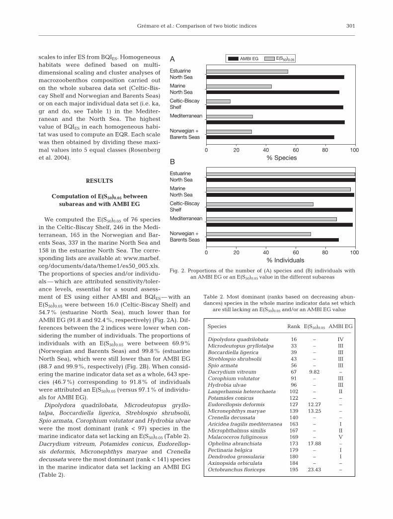
We computed the E(S50)0.05 of 76 speciesin the Celtic-Biscay Shelf, 246 in the Medi-terranean, 165 in the Norwegian and Bar-ents Seas, 337 in the marine North Sea and158 in the estuarine North Sea. The corre-sponding lists are available at: www.marbef.org/documents/data/theme1/es50_005.xls.The proportions of species and/or individu-als — which are attributed sensitivity/toler-ance levels, essential for a sound assess-ment of ES using either AMBI and BQIES— with anE(S50)0.05 were between 16.0 (Celtic-Biscay Shelf) and54.7% (estuarine North Sea), much lower than forAMBI EG (91.8 and 92.4%, respectively) (Fig. 2A). Dif-ferences between the 2 indices were lower when con-sidering the number of individuals. The proportions ofindividuals with an E(S50)0.05 were between 69.9%(Norwegian and Barents Seas) and 99.8% (estuarineNorth Sea), which were still lower than for AMBI EG(88.7 and 99.9%, respectively) (Fig. 2B). When consid-ering the marine indicator data set as a whole, 643 spe-cies (46.7%) corresponding to 91.8% of individualswere attributed an E(S50)0.05 (versus 97.1% of individu-als for AMBI EG).

Dipolydora quadrilobata, Microdeutopus gryllo-talpa, Boccardiella ligerica, Streblospio shrubsolii,Spio armata, Corophium volutator and Hydrobia ulvaewere the most dominant (rank < 97) species in themarine indicator data set lacking an E(S50)0.05 (Table 2).Dacrydium vitreum, Potamides conicus, Eudorellop-sis deformis, Micronephthys maryae and Crenelladecussata were the most dominant (rank < 141) speciesin the marine indicator data set lacking an AMBI EG(Table 2).

301

Norwegian +Barents Seas

Mediterranean

Celtic-BiscayShelf

MarineNorth Sea

EstuarineNorth Sea

AMBI EG E(S50)0.05

% Individuals0 20 40 60 80 100

% Species0 20 40 60 80 100

Norwegian +Barents Seas

Mediterranean

Celtic-BiscayShelf

MarineNorth Sea

EstuarineNorth Sea

A

B

Fig. 2. Proportions of the number of (A) species and (B) individuals withan AMBI EG or an E(S50)0.05 value in the different subareas

Species Rank E(S50)0.05 AMBI EG

Dipolydora quadrilobata 16 – IVMicrodeutopus gryllotalpa 33 – IIIBoccardiella ligerica 39 – IIIStreblospio shrubsolii 43 – IIISpio armata 56 – IIIDacrydium vitreum 67 9.82 –Corophium volutator 91 – IIIHydrobia ulvae 96 – IIILangerhansia heterochaeta 102 – IIPotamides conicus 122 – –Eudorellopsis deformis 127 12.27 –Micronephthys maryae 139 13.25 –Crenella decussata 140 – –Aricidea fragilis mediterranea 163 – IMicrophthalmus similis 167 – IIMalacoceros fuliginosus 169 – VOphelina abranchiata 173 17.88 –Pectinaria belgica 179 – IDendrodoa grossularia 180 – IAxinopsida orbiculata 184 – –Octobranchus floriceps 195 23.43 –

Table 2. Most dominant (ranks based on decreasing abun-dances) species in the whole marine indicator data set which

are still lacking an E(S50)0.05 and/or an AMBI EG value

Mar Ecol Prog Ser 382: 297–311, 2009

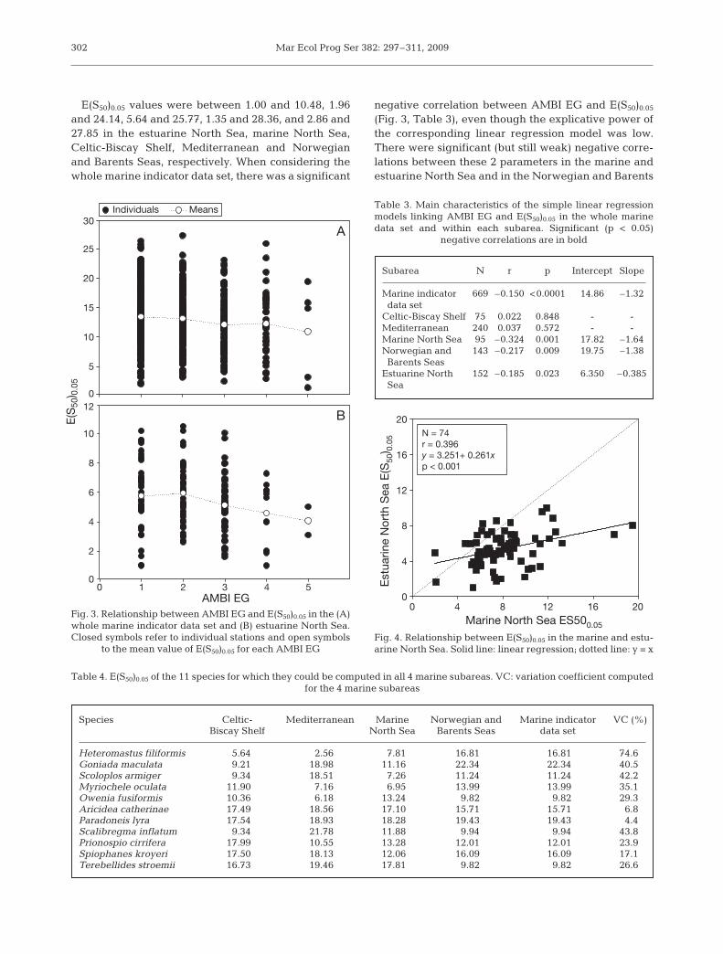
E(S50)0.05 values were between 1.00 and 10.48, 1.96and 24.14, 5.64 and 25.77, 1.35 and 28.36, and 2.86 and27.85 in the estuarine North Sea, marine North Sea,Celtic-Biscay Shelf, Mediterranean and Norwegianand Barents Seas, respectively. When considering thewhole marine indicator data set, there was a significant

negative correlation between AMBI EG and E(S50)0.05

(Fig. 3, Table 3), even though the explicative power ofthe corresponding linear regression model was low.There were significant (but still weak) negative corre-lations between these 2 parameters in the marine andestuarine North Sea and in the Norwegian and Barents

302

Subarea N r p Intercept Slope

Marine indicator 669 –0.150 <0.0001 14.86 –1.32data set

Celtic-Biscay Shelf 75 0.022 0.848 - -Mediterranean 240 0.037 0.572 - -Marine North Sea 95 –0.324 0.001 17.82 –1.64Norwegian and 143 –0.217 0.009 19.75 –1.38Barents Seas

Estuarine North 152 –0.185 0.023 6.350 –0.385Sea

Table 3. Main characteristics of the simple linear regressionmodels linking AMBI EG and E(S50)0.05 in the whole marinedata set and within each subarea. Significant (p < 0.05)

negative correlations are in bold

Species Celtic- Mediterranean Marine Norwegian and Marine indicator VC (%)Biscay Shelf North Sea Barents Seas data set

Heteromastus filiformis 5.64 2.56 7.81 16.81 16.81 74.6Goniada maculata 9.21 18.98 11.16 22.34 22.34 40.5Scoloplos armiger 9.34 18.51 7.26 11.24 11.24 42.2Myriochele oculata 11.90 7.16 6.95 13.99 13.99 35.1Owenia fusiformis 10.36 6.18 13.24 9.82 9.82 29.3Aricidea catherinae 17.49 18.56 17.10 15.71 15.71 6.8Paradoneis lyra 17.54 18.93 18.28 19.43 19.43 4.4Scalibregma inflatum 9.34 21.78 11.88 9.94 9.94 43.8Prionospio cirrifera 17.99 10.55 13.28 12.01 12.01 23.9Spiophanes kroyeri 17.50 18.13 12.06 16.09 16.09 17.1Terebellides stroemii 16.73 19.46 17.81 9.82 9.82 26.6

Table 4. E(S50)0.05 of the 11 species for which they could be computed in all 4 marine subareas. VC: variation coefficient computed for the 4 marine subareas

0

5

10

15

20

25

30

AMBI EG0 1 2 3 4 5

E(S

50) 0

.05

0

2

4

6

8

10

12

Individuals Means

A

B

Fig. 3. Relationship between AMBI EG and E(S50)0.05 in the (A)whole marine indicator data set and (B) estuarine North Sea.Closed symbols refer to individual stations and open symbols

to the mean value of E(S50)0.05 for each AMBI EG

Marine North Sea ES500.05

0 4 8 12 16 20

Est

uarin

e N

orth

Sea

E(S

50) 0.

05

0

4

8

12

16

20N = 74r = 0.396y = 3.251+ 0.261xp < 0.001

Fig. 4. Relationship between E(S50)0.05 in the marine and estu-arine North Sea. Solid line: linear regression; dotted line: y = x

Grémare et al.: Comparison of two biotic indices

Seas (Table 3). This correlation was not significant inthe Mediterranean or in the Celtic-Biscay Shelf, whereAMBI was initially developed.

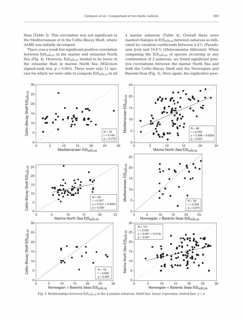
There was a weak but significant positive correlationbetween E(S50)0.05 in the marine and estuarine NorthSea (Fig. 4). However, E(S50)0.05 tended to be lower inthe estuarine than in marine North Sea (Wilcoxonsigned-rank test, p < 0.001). There were only 11 spe-cies for which we were able to compute E(S50)0.05 in all

4 marine subareas (Table 4). Overall there weremarked changes in E(S50)0.05 between subareas as indi-cated by variation coefficients between 4.4% (Parado-neis lyra) and 74.6% (Heteromastus filiformis). Whencomparing the E(S50)0.05 of species occurring in anycombination of 2 subareas, we found significant posi-tive correlations between the marine North Sea andboth the Celtic-Biscay Shelf and the Norwegian andBarents Seas (Fig. 5). Here again, the explicative pow-

303

Mediterranean E(S50)0.05

0

5

10

15

20

25

30

Marine North Sea E(S50)0.05

0

5

10

15

20

25

Norwegian + Barents Seas E(S50)0.05 Norwegian + Barents Seas E(S50)0.05

Norwegian + Barents Seas E(S50)0.05

0 5 10 15 20 25 30 0 5 10 15 20 25 30

0 5 10 15 20 25

0 5 10 15 20 250 5 10 15 20 25 30

0 5 10 15 20 25

Cel

tic-B

isca

y S

helf

E(S

50) 0

.05

Cel

tic-B

isca

y S

helf

E(S

50) 0

.05

Cel

tic-B

isca

y S

helf

E(S

50) 0

.05

0

5

10

15

20

25

30

Marine North Sea E(S50)0.05

Med

iterr

anea

n E

(S50

) 0.0

5

0

5

10

15

20

25

Med

iterr

anea

n E

(S50

) 0.0

5

0

5

10

15

20

25

Mar

ine

Nor

th S

ea E

(S50

) 0.0

5

0

5

10

15

20

25

30

N = 45r = 0.165p = 0.278

N = 98r = 0.456y = 5.398 + 0.620xp < 0.001

N = 60r = 0.357y = 9.047 + 0.620xp = 0.005

N = 30r = 0.330p = 0.075

N = 18r = 0.030p = 0.907

N = 101r = 0.352y = 9.001 + 0.319xp < 0.001

Fig. 5. Relationships between E(S50)0.05 in the 4 marine subareas. Solid line: linear regression, dotted line: y = x

Mar Ecol Prog Ser 382: 297–311, 2009

ers of corresponding simple linear regression modelsalways remained low, and these models differedclearly from the y = x equation. E(S50)0.05 tended to belower in the marine North Sea than in the Celtic-BiscayShelf and the Norwegian and Barents Seas (see Table5 for the significance of corresponding Wilcoxonsigned-rank tests).

Comparisons between AMBI and BQIES

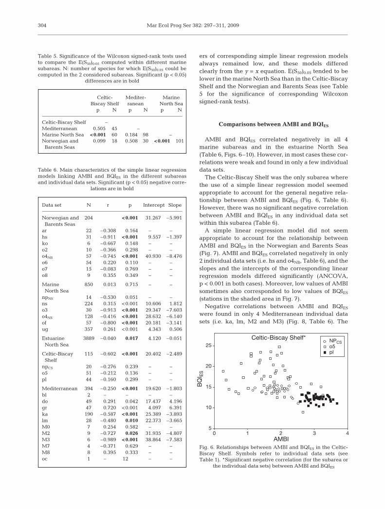
AMBI and BQIES correlated negatively in all 4marine subareas and in the estuarine North Sea(Table 6, Figs. 6–10). However, in most cases these cor-relations were weak and found in only a few individualdata sets.

The Celtic-Biscay Shelf was the only subarea wherethe use of a simple linear regression model seemedappropriate to account for the general negative rela-tionship between AMBI and BQIES (Fig. 6, Table 6).However, there was no significant negative correlationbetween AMBI and BQIES in any individual data setwithin this subarea (Table 6).

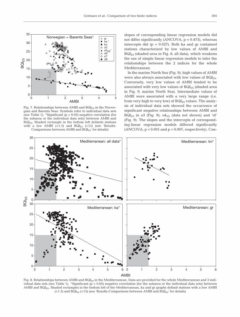
A simple linear regression model did not seemappropriate to account for the relationship betweenAMBI and BQIES in the Norwegian and Barents Seas(Fig. 7). AMBI and BQIES correlated negatively in only2 individual data sets (i.e. hs and o4NB, Table 6), and theslopes and the intercepts of the corresponding linearregression models differed significantly (ANCOVA,p < 0.001 in both cases). Moreover, low values of AMBIsometimes also corresponded to low values of BQIES

(stations in the shaded area in Fig. 7).Negative correlations between AMBI and BQIES

were found in only 4 Mediterranean individual datasets (i.e. ka, lm, M2 and M3) (Fig. 8, Table 6). The

304

Data set N r p Intercept Slope

Norwegian and 204 <0.001 31.267 –5.991Barents Seas

ar 22 –0.308 0.164 – –hs 31 –0.911 <0.001 9.557 –1.397ko 6 –0.667 0.148 – –o2 10 –0.366 0.298 – –o4NB 57 –0.745 <0.001 40.930 –8.476o6 54 0.220 0.110 – –o7 15 –0.083 0.769 – –o8 9 0.355 0.349 – –

Marine 850 0.013 0.715 – –North Sea

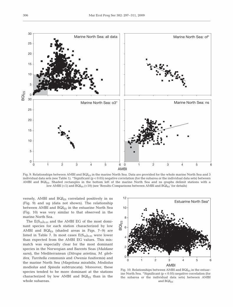
npNS 14 –0.530 0.051 – –ns 224 0.315 <0.001 10.606 1.812o3 30 –0.913 <0.001 29.347 –7.603o4NS 128 –0.416 <0.001 28.632 –6.140of 57 –0.800 <0.001 20.181 –3.141ug 357 0.261 <0.001 4.343 0.506

Estuarine 3889 –0.040 0.017 4.120 –0.051North Sea

Celtic-Biscay 115 –0.602 <0.001 20.402 –2.489Shelf

npCS 20 –0.276 0.239 – –o5 51 –0.212 0.136 – –pl 44 –0.160 0.299 – –

Mediterranean 394 –0.250 <0.001 19.620 –1.803bl 2 – – – –do 49 0.291 0.042 17.437 4.196gr 47 0.720 <0.001 4.097 6.391ka 190 –0.587 <0.001 25.389 –3.893lm 28 –0.480 0.010 22.373 –3.665M0 7 0.254 0.582 – –M2 9 –0.727 0.026 31.935 –4.807M3 6 –0.989 <0.001 38.864 –7.583M7 4 –0.371 0.629 – –M8 8 0.395 0.333 – –oc 1 – 12 – –

Table 6. Main characteristics of the simple linear regressionmodels linking AMBI and BQIES in the different subareasand individual data sets. Significant (p < 0.05) negative corre-

lations are in bold

Celtic- Mediter- MarineBiscay Shelf ranean North Sea

p N p N p N

Celtic-Biscay Shelf –Mediterranean 0.505 45 –Marine North Sea <0.001 60 0.184 98 –Norwegian and 0.099 18 0.508 30 <0.001 101Barents Seas

Table 5. Significance of the Wilcoxon signed-rank tests usedto compare the E(S50)0.05 computed within different marinesubareas. N: number of species for which E(S50)0.05 could becomputed in the 2 considered subareas. Significant (p < 0.05)

differences are in bold

AMBI0 1 2 3 4

BQ

I ES

5

10

15

20

25NPCSo5 pl

Celtic-Biscay Shelf*

Fig. 6. Relationships between AMBI and BQIES in the Celtic-Biscay Shelf. Symbols refer to individual data sets (seeTable 1). *Significant negative correlation (for the subarea or

the individual data sets) between AMBI and BQIES

Grémare et al.: Comparison of two biotic indices

slopes of corresponding linear regression models didnot differ significantly (ANCOVA, p = 0.473), whereasintercepts did (p = 0.027). Both ka and gr containedstations characterized by low values of AMBI andBQIES (shaded area in Fig. 8, all data), which weakensthe use of simple linear regression models to infer therelationships between the 2 indices for the wholeMediterranean.

In the marine North Sea (Fig. 9), high values of AMBIwere also always associated with low values of BQIES.Conversely, very low values of AMBI tended to beassociated with very low values of BQIES (shaded areain Fig. 9, marine North Sea). Intermediate values ofAMBI were associated with a very large range (i.e.from very high to very low) of BQIES values. The analy-sis of individual data sets showed the occurrence ofsignificant negative relationships between AMBI andBQIES in o3 (Fig. 9), o4NS (data not shown) and ‘of’(Fig. 9). The slopes and the intercepts of correspond-ing linear regression models differed significantly(ANCOVA, p < 0.001 and p = 0.007, respectively). Con-

305

0 1 2AMBI

3 4 5

BQ

I ES

0

5

10

15

20

25

30

35Norwegian + Barents Seas* ar

hs *koo2 o4NB*o6 o7 o8

Fig. 7. Relationships between AMBI and BQIES in the Norwe-gian and Barents Seas. Symbols refer to individual data sets(see Table 1). *Significant (p < 0.05) negative correlation (forthe subarea or the individual data sets) between AMBI andBQIES. Shaded rectangle in the bottom left delimits stationswith a low AMBI (<1.5) and BQIES (<15) (see ‘Results-

Comparisons between AMBI and BQIES’ for details)

0

5

10

15

20

25

30Mediterranean: all data* Mediterranean: lm*

Mediterranean: gr

AMBI

0 1 2 3 4 5 6 0 1 2 3 4 5 6

BQ

I ES

0

5

10

15

20

25

30Mediterranean: ka*

Fig. 8. Relationships between AMBI and BQIES in the Mediterranean. Data are provided for the whole Mediterranean and 3 indi-vidual data sets (see Table 1). *Significant (p < 0.05) negative correlation (for the subarea or the individual data sets) betweenAMBI and BQIES. Shaded rectangles in the bottom left of the Mediterranean, ka and gr graphs delimit stations with a low AMBI

(<1.5) and BQIES (<15) (see ‘Results-Comparisons between AMBI and BQIES’ for details)

Mar Ecol Prog Ser 382: 297–311, 2009

versely, AMBI and BQIES correlated positively in ns(Fig. 9) and ug (data not shown). The relationshipbetween AMBI and BQIES in the estuarine North Sea(Fig. 10) was very similar to that observed in themarine North Sea.

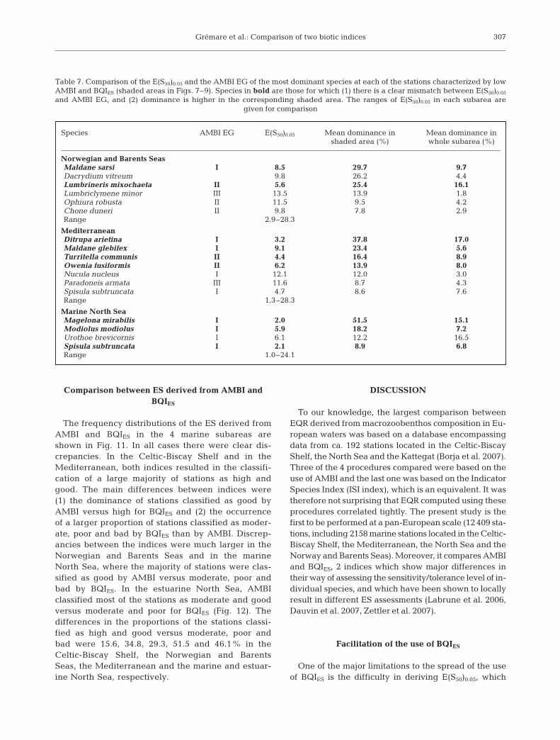
The E(S50)0.05 and the AMBI EG of the most domi-nant species for each station characterized by lowAMBI and BQIES (shaded areas in Figs. 7–9) arelisted in Table 7. In most cases E(S50)0.05 were lowerthan expected from the AMBI EG values. This mis-match was especially clear for the most dominantspecies in the Norwegian and Barents Seas (Maldanesarsi), the Mediterranean (Ditrupa arietina, M. gleb-ifex, Turritella communis and Owenia fusiformis) andthe marine North Sea (Magelona mirabilis, Modiolusmodiolus and Spisula subtruncata). Moreover, thesespecies tended to be more dominant at the stationscharacterized by low AMBI and BQIES than in thewhole subareas.

306

0

5

10

15

20

25

30Marine North Sea: all data Marine North Sea: of*

Marine North Sea: ns

AMBI0 1 2 3 4 5 6 0 1 2 3 4 5 6

BQ

I ES

0

5

10

15

20

25

30Marine North Sea: o3*

Fig. 9. Relationships between AMBI and BQIES in the marine North Sea. Data are provided for the whole marine North Sea and 3individual data sets (see Table 1). *Significant (p < 0.05) negative correlation (for the subarea or the individual data sets) betweenAMBI and BQIES. Shaded rectangles in the bottom left of the marine North Sea and ns graphs delimit stations with a

low AMBI (<1) and BQIES (<10) (see ‘Results-Comparisons between AMBI and BQIES’ for details)

AMBI0 1 2 3 4 5 6

BQ

I ES

0

2

4

6

8

10

12Estuarine North Sea*

Fig. 10. Relationships between AMBI and BQIES in the estuar-ine North Sea. *Significant (p < 0.05) negative correlation (forthe subarea or the individual data sets) between AMBI

and BQIES

Grémare et al.: Comparison of two biotic indices

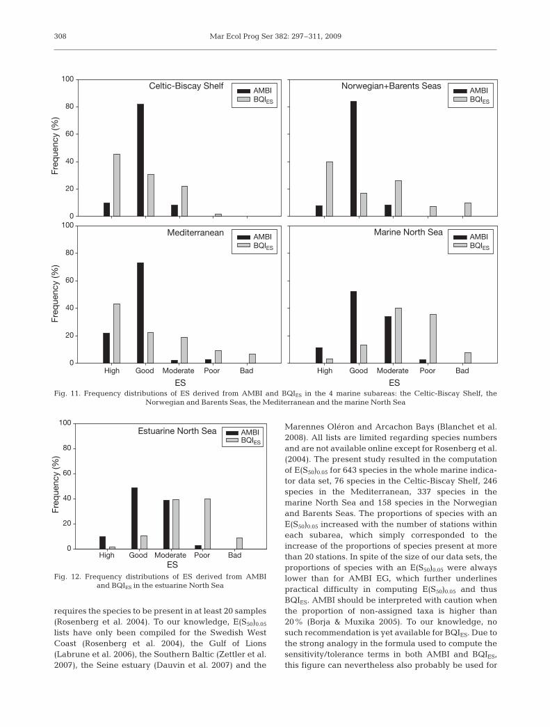
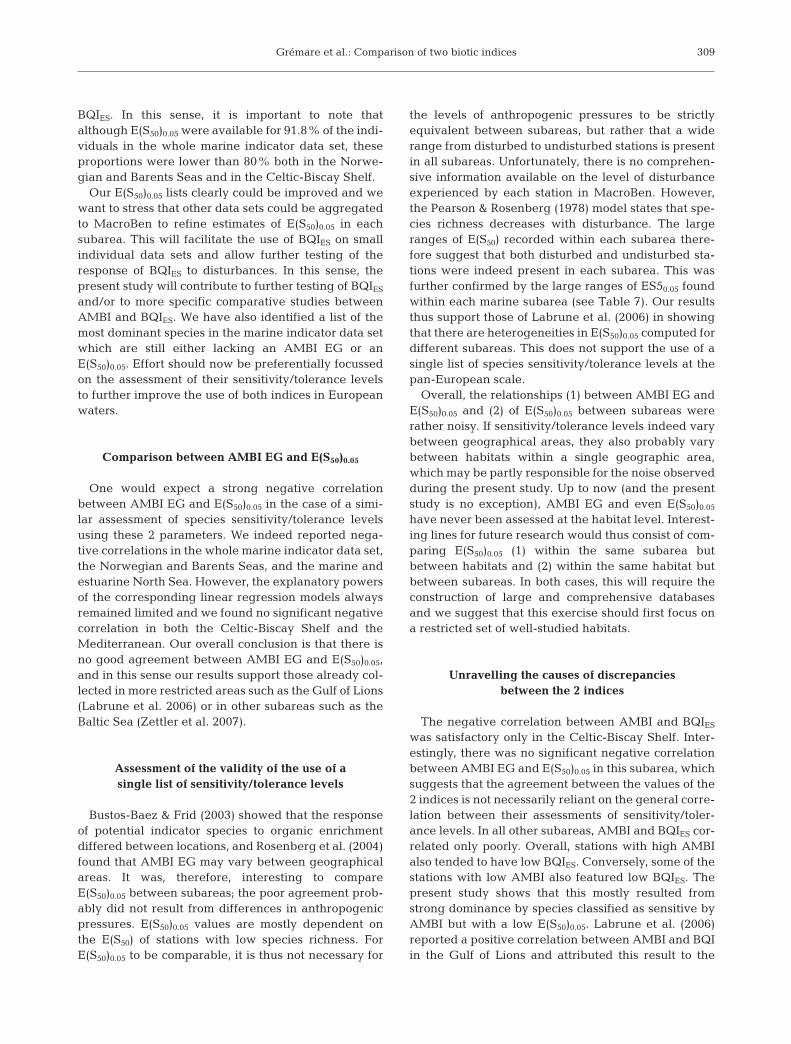
Comparison between ES derived from AMBI andBQIES

The frequency distributions of the ES derived fromAMBI and BQIES in the 4 marine subareas areshown in Fig. 11. In all cases there were clear dis-crepancies. In the Celtic-Biscay Shelf and in theMediterranean, both indices resulted in the classifi-cation of a large majority of stations as high andgood. The main differences between indices were(1) the dominance of stations classified as good byAMBI versus high for BQIES and (2) the occurrenceof a larger proportion of stations classified as moder-ate, poor and bad by BQIES than by AMBI. Discrep-ancies between the indices were much larger in theNorwegian and Barents Seas and in the marineNorth Sea, where the majority of stations were clas-sified as good by AMBI versus moderate, poor andbad by BQIES. In the estuarine North Sea, AMBIclassified most of the stations as moderate and goodversus moderate and poor for BQIES (Fig. 12). Thedifferences in the proportions of the stations classi-fied as high and good versus moderate, poor andbad were 15.6, 34.8, 29.3, 51.5 and 46.1% in theCeltic-Biscay Shelf, the Norwegian and BarentsSeas, the Mediterranean and the marine and estuar-ine North Sea, respectively.

DISCUSSION

To our knowledge, the largest comparison betweenEQR derived from macrozoobenthos composition in Eu-ropean waters was based on a database encompassingdata from ca. 192 stations located in the Celtic-BiscayShelf, the North Sea and the Kattegat (Borja et al. 2007).Three of the 4 procedures compared were based on theuse of AMBI and the last one was based on the IndicatorSpecies Index (ISI index), which is an equivalent. It wastherefore not surprising that EQR computed using theseprocedures correlated tightly. The present study is thefirst to be performed at a pan-European scale (12 409 sta-tions, including 2158 marine stations located in the Celtic-Biscay Shelf, the Mediterranean, the North Sea and theNorway and Barents Seas). Moreover, it compares AMBIand BQIES, 2 indices which show major differences intheir way of assessing the sensitivity/tolerance level of in-dividual species, and which have been shown to locallyresult in different ES assessments (Labrune et al. 2006,Dauvin et al. 2007, Zettler et al. 2007).

Facilitation of the use of BQIES

One of the major limitations to the spread of the useof BQIES is the difficulty in deriving E(S50)0.05, which

307

Species AMBI EG E(S50)0.05 Mean dominance in Mean dominance inshaded area (%) whole subarea (%)

Norwegian and Barents SeasMaldane sarsi I 8.5 29.7 9.7Dacrydium vitreum 9.8 26.2 4.4Lumbrineris mixochaeta II 5.6 25.4 16.1Lumbriclymene minor III 13.5 13.9 1.8Ophiura robusta II 11.5 9.5 4.2Chone duneri II 9.8 7.8 2.9Range 2.9–28.3

MediterraneanDitrupa arietina I 3.2 37.8 17.0Maldane glebifex I 9.1 23.4 5.6Turritella communis II 4.4 16.4 8.9Owenia fusiformis II 6.2 13.9 8.0Nucula nucleus I 12.1 12.0 3.0Paradoneis armata III 11.6 8.7 4.3Spisula subtruncata I 4.7 8.6 7.6Range 1.3–28.3

Marine North SeaMagelona mirabilis I 2.0 51.5 15.1Modiolus modiolus I 5.9 18.2 7.2Urothoe brevicornis I 6.1 12.2 16.5Spisula subtruncata I 2.1 8.9 6.8Range 1.0–24.1

Table 7. Comparison of the E(S50)0.05 and the AMBI EG of the most dominant species at each of the stations characterized by lowAMBI and BQIES (shaded areas in Figs. 7–9). Species in bold are those for which (1) there is a clear mismatch between E(S50)0.05

and AMBI EG, and (2) dominance is higher in the corresponding shaded area. The ranges of E(S50)0.05 in each subarea are given for comparison

Mar Ecol Prog Ser 382: 297–311, 2009

requires the species to be present in at least 20 samples(Rosenberg et al. 2004). To our knowledge, E(S50)0.05

lists have only been compiled for the Swedish WestCoast (Rosenberg et al. 2004), the Gulf of Lions(Labrune et al. 2006), the Southern Baltic (Zettler et al.2007), the Seine estuary (Dauvin et al. 2007) and the

Marennes Oléron and Arcachon Bays (Blanchet et al.2008). All lists are limited regarding species numbersand are not available online except for Rosenberg et al.(2004). The present study resulted in the computationof E(S50)0.05 for 643 species in the whole marine indica-tor data set, 76 species in the Celtic-Biscay Shelf, 246species in the Mediterranean, 337 species in themarine North Sea and 158 species in the Norwegianand Barents Seas. The proportions of species with anE(S50)0.05 increased with the number of stations withineach subarea, which simply corresponded to theincrease of the proportions of species present at morethan 20 stations. In spite of the size of our data sets, theproportions of species with an E(S50)0.05 were alwayslower than for AMBI EG, which further underlinespractical difficulty in computing E(S50)0.05 and thusBQIES. AMBI should be interpreted with caution whenthe proportion of non-assigned taxa is higher than20% (Borja & Muxika 2005). To our knowledge, nosuch recommendation is yet available for BQIES. Due tothe strong analogy in the formula used to compute thesensitivity/tolerance terms in both AMBI and BQIES,this figure can nevertheless also probably be used for

308

Freq

uenc

y (%

)Fr

eque

ncy

(%)

0

20

40

60

80

100

AMBIBQIES

Celtic-Biscay Shelf AMBIBQIES

Norwegian+Barents Seas

Mediterranean

ES

AMBIBQIES

Marine North Sea

ESHigh Good Moderate Poor Bad High Good Moderate Poor Bad

0

20

40

60

80

100

AMBIBQIES

Fig. 11. Frequency distributions of ES derived from AMBI and BQIES in the 4 marine subareas: the Celtic-Biscay Shelf, the Norwegian and Barents Seas, the Mediterranean and the marine North Sea

ESHigh Good Moderate Poor Bad

Freq

uenc

y (%

)

0

20

40

60

80

100AMBIBQIES

Estuarine North Sea

Fig. 12. Frequency distributions of ES derived from AMBI and BQIES in the estuarine North Sea

Grémare et al.: Comparison of two biotic indices

BQIES. In this sense, it is important to note thatalthough E(S50)0.05 were available for 91.8% of the indi-viduals in the whole marine indicator data set, theseproportions were lower than 80% both in the Norwe-gian and Barents Seas and in the Celtic-Biscay Shelf.

Our E(S50)0.05 lists clearly could be improved and wewant to stress that other data sets could be aggregatedto MacroBen to refine estimates of E(S50)0.05 in eachsubarea. This will facilitate the use of BQIES on smallindividual data sets and allow further testing of theresponse of BQIES to disturbances. In this sense, thepresent study will contribute to further testing of BQIES

and/or to more specific comparative studies betweenAMBI and BQIES. We have also identified a list of themost dominant species in the marine indicator data setwhich are still either lacking an AMBI EG or anE(S50)0.05. Effort should now be preferentially focussedon the assessment of their sensitivity/tolerance levelsto further improve the use of both indices in Europeanwaters.

Comparison between AMBI EG and E(S50)0.05

One would expect a strong negative correlationbetween AMBI EG and E(S50)0.05 in the case of a simi-lar assessment of species sensitivity/tolerance levelsusing these 2 parameters. We indeed reported nega-tive correlations in the whole marine indicator data set,the Norwegian and Barents Seas, and the marine andestuarine North Sea. However, the explanatory powersof the corresponding linear regression models alwaysremained limited and we found no significant negativecorrelation in both the Celtic-Biscay Shelf and theMediterranean. Our overall conclusion is that there isno good agreement between AMBI EG and E(S50)0.05,and in this sense our results support those already col-lected in more restricted areas such as the Gulf of Lions(Labrune et al. 2006) or in other subareas such as theBaltic Sea (Zettler et al. 2007).

Assessment of the validity of the use of a single list of sensitivity/tolerance levels

Bustos-Baez & Frid (2003) showed that the responseof potential indicator species to organic enrichmentdiffered between locations, and Rosenberg et al. (2004)found that AMBI EG may vary between geographicalareas. It was, therefore, interesting to compareE(S50)0.05 between subareas; the poor agreement prob-ably did not result from differences in anthropogenicpressures. E(S50)0.05 values are mostly dependent onthe E(S50) of stations with low species richness. ForE(S50)0.05 to be comparable, it is thus not necessary for

the levels of anthropogenic pressures to be strictlyequivalent between subareas, but rather that a widerange from disturbed to undisturbed stations is presentin all subareas. Unfortunately, there is no comprehen-sive information available on the level of disturbanceexperienced by each station in MacroBen. However,the Pearson & Rosenberg (1978) model states that spe-cies richness decreases with disturbance. The largeranges of E(S50) recorded within each subarea there-fore suggest that both disturbed and undisturbed sta-tions were indeed present in each subarea. This wasfurther confirmed by the large ranges of ES50.05 foundwithin each marine subarea (see Table 7). Our resultsthus support those of Labrune et al. (2006) in showingthat there are heterogeneities in E(S50)0.05 computed fordifferent subareas. This does not support the use of asingle list of species sensitivity/tolerance levels at thepan-European scale.

Overall, the relationships (1) between AMBI EG andE(S50)0.05 and (2) of E(S50)0.05 between subareas wererather noisy. If sensitivity/tolerance levels indeed varybetween geographical areas, they also probably varybetween habitats within a single geographic area,which may be partly responsible for the noise observedduring the present study. Up to now (and the presentstudy is no exception), AMBI EG and even E(S50)0.05

have never been assessed at the habitat level. Interest-ing lines for future research would thus consist of com-paring E(S50)0.05 (1) within the same subarea butbetween habitats and (2) within the same habitat butbetween subareas. In both cases, this will require theconstruction of large and comprehensive databasesand we suggest that this exercise should first focus ona restricted set of well-studied habitats.

Unravelling the causes of discrepancies between the 2 indices

The negative correlation between AMBI and BQIES

was satisfactory only in the Celtic-Biscay Shelf. Inter-estingly, there was no significant negative correlationbetween AMBI EG and E(S50)0.05 in this subarea, whichsuggests that the agreement between the values of the2 indices is not necessarily reliant on the general corre-lation between their assessments of sensitivity/toler-ance levels. In all other subareas, AMBI and BQIES cor-related only poorly. Overall, stations with high AMBIalso tended to have low BQIES. Conversely, some of thestations with low AMBI also featured low BQIES. Thepresent study shows that this mostly resulted fromstrong dominance by species classified as sensitive byAMBI but with a low E(S50)0.05. Labrune et al. (2006)reported a positive correlation between AMBI and BQIin the Gulf of Lions and attributed this result to the

309

Mar Ecol Prog Ser 382: 297–311, 2009

strong dominance of the serpulid polychaete Ditrupaarietina (Grémare et al. 1998, Labrune et al. 2007a),which was classified as sensitive by AMBI and had alow E(S50)0.05. Our results support this interpretationand generalize it to other geographical areas (e.g. theCretan Shelf) and to other species. The present studyprovides the first lists of the most dominant specieswithin each marine subarea for which there are impor-tant discrepancies between AMBI EG and E(S50)0.05.All were classified in AMBI EG I or II. However, someof them are known to be influenced by natural sourcesof disturbance such as sediment instability (D. arietina,Grémare et al. 1998 and Magelona mirabilis, Rayment2007) or climatic anomalies (Maldane glebifex, Glé-marec et al. 1986) and cycles (D. arietina, Labrune etal. 2007b). These observations are indicative of thetendency of E(S50)0.05 to automatically classify domi-nant species as tolerant and its inability to differentiatebetween natural and anthropogenic sources of distur-bance (Labrune et al. 2006, 2007b). Further autoeco-logical studies are nevertheless clearly needed to bet-ter unravel the actual sensitivity/tolerance levels of thespecies highlighted in Table 7.

Comparison of ES assessments derived from AMBI and BQIES

Given the discrepancies between AMBI and BQIES,it was not surprising that the frequency distributionsof ES derived from these 2 indices differed in mostsubareas. In the Norwegian and Barents Seas andboth the marine and estuarine North Sea, these dis-crepancies were also apparent when distinguishingstations with a high or good ES from those with amoderate, poor or bad ES as recommended by theWFD. BQIES resulted in overall poorer ES than AMBI,which supports preliminary results in the Gulf ofLions (Labrune et al. 2006), the Southern Baltic(Zettler et al. 2007) the Bay of Seine (Dauvin et al.2007) and to a lesser extent the North Sea (Reiss &Kröncke 2005).

It should be underlined that all the above-mentionedstudies plus the present one have used a fixed con-version scale to infer ES from AMBI. One of the charac-teristics of the recently introduced M-AMBI is that itis using a different conversion scale for each homo-geneous habitat as does BQIES (Borja et al. 2007,Muxika et al. 2007a). In both cases, this requires theexistence of valid references (i.e. a single high refer-ence in the case of BQIES, and both a bad and a highreference in the case of M-AMBI). The computation ofM-AMBI was not integrated in the MacroBen tool andwe did not use this procedure to infer ES during thepresent study.

CONCLUSIONS

AMBI and BQIES both ultimately rely on species sen-sitivity/tolerance levels, which they respectively assessthrough AMBI EG and E(S50)0.05. We identified themost dominant species in marine European waters stilllacking an AMBI EG or an E(S50)0.05. Our results sup-port those of previous studies, obtained at muchsmaller geographical scales, in showing that AMBI EGand E(S50)0.05 poorly agree. They suggest that the useof a single sensitivity/tolerance list in different geo-graphical areas (such as in AMBI EG) is not appropri-ate. Discrepancies between the values of the 2 indicesare due to the dominance of species characterized assensitive by AMBI and tolerant by BQIES. These spe-cies were identified and some of them are known to beinfluenced by natural disturbance, which highlightsthe tendency of BQIES to classify dominant species astolerant and thus to be inefficient in distinguishinganthropogenic from natural disturbances. AMBI andBQIES thus both present weaknesses relative to theassessment of sensitivity/tolerance. Both indices havebeen subject to several recent refinements regardingtheir computation and their procedures to infer ES,which are now quite comparable. However, all thesesteps are posterior (and thus dependent on) a soundassessment of species sensitivity/tolerance. Changes inthe scales used to convert indices to ES can only par-tially compensate for changes in sensitivity/tolerancelevels among geographical areas and/or habitats. Pref-erential attention should thus now be paid to this par-ticular issue. Future studies should focus on (1) theclarification of the sensitivity/tolerance levels of thespecies identified as problematic during the presentstudy, and (2) the assessment of the relationshipsbetween AMBI EG and E(S50)0.05 within and betweencombinations of geographical areas and habitats.

Acknowledgements. This study was carried out within theframework of the EU Network of Excellence Marine Biodiver-sity and Ecoystem Functioning (MarBEF). We thank F. Aleffi,A. Koukouras, R. Jasku8a, A. S. Y. Mackie, P. G. Oliver, E. I. S.Rees, J. M. Wes8awski, J. Wittoeck, the Norwegian Oil Indus-try Association, Akvaplan-niva and Det Norske Veritas forkindly providing data. We deeply thank C. Arvinitidis fororganising the 2005 MarBEF Theme 1 Crete workshop wherethis work was initiated.

LITERATURE CITED

Bigot L, Grémare A, Amouroux JM, Frouin P (2008) Assess-ment of the ecological quality status of soft-bottoms inRéunion Island (Southwest Indian Ocean) using both AZTIMarine Biotic Indices. Mar Pollut Bull 56:704–722

Blanchet H, Lavesque N, Ruellet T, Dauvin JC and others(2008) Use of biotic indices in semi-enclosed coastalecosystems and transitional waters habitats: implications

310

Grémare et al.: Comparison of two biotic indices

for the implementation of the European Water FrameworkDirective. Ecol Indic 8:360–372

Borja A (2005) The European Water Framework Directive: achallenge for nearshore, coastal and continental shelfresearch. Cont Shelf Res 25:1768–1783

Borja A, Muxika I (2005) Guidelines for the use of AMBI(AZTI’s Marine Biotic Index) in the assessment of the ben-thic ecological quality. Mar Pollut Bull 50:787–789

Borja A, Franco J, Pérez V (2000) A marine biotic index toestablish the ecological quality of soft-bottom benthoswithin European estuarine and coastal environments. MarPollut Bull 40:1100–1114

Borja A, Muxika I, Franco J (2003) The application of a marinebiotic index to different impact sources affecting soft-bot-tom benthic communities along European coasts. Mar Pol-lut Bull 46:835–845

Borja A, Franco J, Valencia V, Bald J, Muxika I, Belzunce MJ,Slaun O (2004a) Implementation of the European waterframework directive from the Basque country (northernSpain): a methodological approach. Mar Pollut Bull48:209–218

Borja A, Franco J, Muxika I (2004b) The biotic indices and theWater Framework Directive: the required consensus in thenew benthic monitoring tools. Mar Pollut Bull 48:405–408

Borja A, Josefson AB, Miles A, Muxika I and others (2007) Anapproach to the intercalibration of benthic ecological sta-tus assessment in the North Atlantic ecoregion, accordingto the European Water Framework Directive. Mar PollutBull 55:42–52

Bustos-Baez S, Frid C (2003) Using indicator species to assessthe state of macrobenthic communities. Hydrobiologia496:299–309

Dauvin JC, Ruellet T, Desroy N, Janson AL (2007) The ecolog-ical quality status of the Bay of Seine and the Seine estu-ary: use of biotic indices. Mar Pollut Bull 55:241–257

Diaz RJ, Solan M, Valente RM (2004) A review of approachesfor classifying benthic habitats and evaluating habitatquality. J Environ Manage 73:165–181

Fleischer D, Grémare A, Labrune C, Rumohr H, VandenBerghe E, Zettler ML (2007) Performance comparison oftwo biotic indices measuring the ecological status of waterbodies in the Southern Baltic and the Gulf of Lions. MarPollut Bull 54:1598–1606

Glémarec M, Le Bris H, Le Guellec C (1986) Modifications desécosystèmes des vasières côtières du sud-Bretagne.Hydrobiologia 142:159–170 (In French with Englishabstract)

Gomez Gesteira JL, Dauvin JC (2000) Amphipods are goodbioindicators of the impact of oil spills on soft-bottom mac-robenthic communities. Mar Pollut Bull 40:1017–1027

Grall J, Glémarec M (1997) Using biotic indices to estimatemacrobenthic community perturbations in the Bay ofBrest. Estuar Coast Shelf Sci 44(Suppl A):43–53

Grémare A, Sardá R, Medernach L, Jordana E and others(1998) On the dramatic increase of Ditrupa arietina O.F.Müller (Annelida: Polychaeta) along both the French andSpanish Catalan coasts. Estuar Coast Shelf Sci 47:447–457

Hurlbert SH (1971) The nonconcept of species diversity: a cri-tique and alternative parameters. Ecology 52:577–586

Labrune C, Amouroux JM, Sardá R, Dutrieux E, Thorin S,Rosenberg R, Grémare A (2006) Characterization of theecological quality of the coastal Gulf of Lions (NWMediterranean). A comparative approach based on threebiotic indices. Mar Pollut Bull 52:34–47

Labrune C, Grémare A, Amouroux JM, Sardá R, Gil J,Taboada S (2007a) Assessment of soft-bottom polychaeteassemblages in the Gulf of Lions (NW Mediterranean)based on a mesoscale survey. Estuar Coast Shelf Sci71:133–147

Labrune C, Grémare A, Guizien K, Amouroux JM (2007b)Long-term comparison of soft bottom macrobenthos in theBay of Banyuls-sur-Mer (north-western MediterraneanSea): a reappraisal. J Sea Res 58:125–143

Marin-Guirao L, Cesar A, Marin A, Lloret J, Vita R (2005)Establishing the ecological quality status of soft-bottommining-impacted coastal water bodies in the scope of theWater Framework Directive. Mar Pollut Bull 50:374–387

Muniz P, Venturini N, Pires-Vanin AMS, Tommasi LR, Borja A(2005) Testing the applicability of a marine biotic index(AMBI) to assessing the ecological quality of soft-bottombenthic communities, in the South America Atlanticregion. Mar Pollut Bull 50:624–637

Muxika I, Borja A, Bonne W (2005) The suitability of themarine biotic index (AMBI) to new impact sources alongEuropean coasts. Ecol Indic 5:19–31

Muxika I, Borja A, Bald J (2007a) Using historical data, expertjudgement and multivariate analysis in assessing refer-ence conditions and benthic ecological status, accordingto the European Water Framework Directive. Mar PollutBull 55:16–29

Muxika I, Ibaibarriaga L, Saiz JI, Borja A (2007b) Minimalsampling requirements for a precise assessment of soft-bottom macrobenthic communities, using AMBI. J ExpMar Biol Ecol 349:323–333

Pearson TH, Rosenberg R (1978) Macrobenthic succession inrelation to organic enrichment and pollution of the marineenvironment. Oceanogr Mar Biol Annu Rev 16:229–311

Rayment WJ (2007) Magelona mirabilis. A polychaete.Marine Life Information Network: Biology and SensitivityKey Information Sub-programme. Mar Biol Assoc UK, Ply-mouth. Available at www.marlin.ac.uk/species/Magelon-amirabilis.htm

Reiss H, Kröncke I (2005) Seasonal variability of benthicindices: An approach to test the applicability of differentindices for ecosystem quality assessment. Mar Pollut Bull50:1490–1499

Rosenberg R, Blomqvist M, Nilsson HC, Cederwall H, Dim-ming A (2004) Marine quality assessment by use of ben-thic species-abundance distributions: a proposed new pro-tocol within the European Union Water FrameworkDirective. Mar Pollut Bull 49:728–739

Salas F, Neto JM, Borja A, Marques JC (2004) Evaluation ofthe applicability of a marine biotic index to characterizethe status of estuarine ecosystems: the case of Mondegoestuary (Portugal). Ecol Indic 4:215–225

Vanden Berghe E, Claus S, Appeltans W, Faulwetter S andothers (2009) MacroBen integrated database on benthicinvertebrates of European continental shelves: a tool forlarge-scale analysis across Europe. Mar Ecol Prog Ser 382:225–238

Wallin M, Wiederholm T, Johnson RK (2003) Guidance onestablishing reference conditions and ecological statusclass boundaries for inland surface waters. CommonImplementation Strategy Working Group 2.3, REFCOND,Water Framework Directive, Luxembourg

Zettler ML, Schiedek D, Bobertz B (2007) Benthic biodiversityindices versus salinity gradient in the southern Baltic Sea.Mar Pollut Bull 55:258–270

311

Submitted: June 5, 2008; Accepted: March 25, 2009 Proofs received from author(s): April 23, 2009