�����������������

Citation: Cheng, T.; Lu, D.D.-C.;

Siwakoti, Y.P. Circuit-Based Rainflow

Counting Algorithm in Application

of Power Device Lifetime Estimation.

Energies 2022, 15, 5159. https://

doi.org/10.3390/en15145159

Received: 15 June 2022

Accepted: 13 July 2022

Published: 16 July 2022

Publisher’s Note: MDPI stays neutral

with regard to jurisdictional claims in

published maps and institutional affil-

iations.

Copyright: © 2022 by the authors.

Licensee MDPI, Basel, Switzerland.

This article is an open access article

distributed under the terms and

conditions of the Creative Commons

Attribution (CC BY) license (https://

creativecommons.org/licenses/by/

4.0/).

energies

Article

Circuit-Based Rainflow Counting Algorithm in Application ofPower Device Lifetime EstimationTian Cheng *, Dylan Dah-Chuan Lu and Yam P. Siwakoti

School of Electrical and Data Engineering, Faculty of Engineering and IT, University of Technology Sydney,Building 11, Ultimo, NSW 2007, Australia; Dylan.lu@uts.edu.au (D.D.-C.L.); Yam.Siwakoti@uts.edu.au (Y.P.S.)* Correspondence: Tian.Cheng@student.uts.edu.au

Abstract: The software-assisted reliability assessment of power electronic converters is increasinglyimportant due to its multi-domain nature and extensive parametric calculations. The rainflowcounting algorithm is gaining popularity for its low relative error in device lifetime estimation.Nevertheless, the offline operation of the algorithm prevents most simulation software packagesconsidering other parameters for the device under study, such as aging and the current state ofhealth in the estimation, as it requires a complete loading profile to run recursive comparison. Thisalso brings difficulties in realization in circuit simulators such as SPICE. To tackle the issue, anin-the-loop circuit-based rainflow counting algorithm is proposed in this paper, and applied toestimate the consumed lifetime of the MOSFET in a boost converter for illustration. Instantaneouselectrical and thermal performances, and the accumulated stress of the device can be monitored.Not only does this assist in evaluating the state of health of a device, but also allows the possibilityof integrating the aging into the lifetime evaluation. The method follows the four-point rainflowcounting algorithms, which continuously compares three adjacent temperature fluctuations ∆Tj toselect full cycles for two rounds, and the remaining cycles are counted as half cycles. To validatethe performance, a comparative analysis in terms of counting accuracy and simulation speed wasperformed alongside the proposed method, MATLAB® and also with a well-accepted half-cyclecounting method. Reported results show that the proposed method has an improved countingaccuracy compared to the half-cycle counting from 24% to 3.5% on average under different loadstresses and length conditions. The accuracy can be effectively improved by a further 1.3–2% byadding an extra comparison round.

Keywords: circuit-based rainflow counting algorithm; multi-domain simulation; lifetime estima-tion application

1. Introduction

Stress cycle counting algorithms translate complicated and irregular loading profilesinto a set of organized cycles to facilitate stress accumulative calculations, and are essen-tial in reliability assessments and lifetime prediction for power devices, such as powersemiconductors, or converters/inverters, especially when they operate with critical andvarying loads.

Various counting approaches such as level-crossing, peak counting and rainflow wereintroduced in [1–5]. Comparative discussions on peak counting algorithms (e.g., half-cycle,maximum edge and rising edge) and rainflow counting are given in [6] through thermo-mechanical FEM analysis, and the rainflow counting is reported to have the lowest relativeerror with 11% while the others are between 19–27% when running a certain missionprofile. Rainflow counting was first introduced by Matsuishi and Endo in fatigue analysisin 1968 [7] by assuming the reversals as rain drops and drips off the pagoda roofs. Thismethod incorporates closed hysteresis loops in stress–strain plots and considers them tobe full cycles with corresponding range and mean value. It has also gained popularity in

Energies 2022, 15, 5159. https://doi.org/10.3390/en15145159 https://www.mdpi.com/journal/energies

Energies 2022, 15, 5159 2 of 13

dealing with critical thermal profiles and calculating lifetimes. For example, the lifetimeof grid-connected PV inverters in [8,9], multi-level converters utilized in wind turbinesystems [10–12] are evaluated with the help of this counting algorithm. In most of thesestudies, the counting is completed by inputting the thermal profile into the MATLAB®

rainflow counting command for ease of implementation and fast computation speed. Tothe best of our knowledge, there are very few existing solutions which realize rainflowcounting in a circuit simulation platform. Possible reasons may be that the traditionalrainflow method is applied offline, while the circuit simulator follows the time sequence,which brings difficulties in comparing different reversals, especially when they are far awayfrom each other.

There is a growing trend at present for implementing multi-domain or multi-disciplinesimulations; for instance, an increasing number of integrated electro-thermal models ofpower MOSFETs, IGBTs, etc., are provided by leading manufacturers such as Infineonand STMicroelectronics. It could be beneficial to include lifetime estimation into thesimulation, such that users are allowed to monitor the device’s electrical performance,thermal properties, accumulated damage and lifetime simultaneously and only in onesimulator. Apart from this, studies have demonstrated the great impacts of aging andthe current health state of a device on lifetime estimation [13–17]. To take them intoconsideration, it is necessary to know the instantaneous accumulated stress. In otherwords, an online counting method is required. Although the MATLAB® rainflow countingfunction provides a convenient implementation, it is an offline method which means acomplete loading profile is required. To tackle this, online rainflow counting methods wereproposed in [18,19]. All are stack-based recursive algorithms, which allow users to easilyselect and discard counted cycles in programming. These methods are well-suited to areal-time environment but have difficulty in being applied in a circuit simulator. As circuitsimulators follow the time sequence, it is not possible to make any change on those alreadyplotted points.

This paper proposes an easy-to-use and in-the-loop rainflow counting approach forpower devices and power electronic circuits. The novelty of the proposed work is theimplementation of the algorithm in a circuit simulator, which makes possible the in-the-loop monitoring of the electrical and thermal performances, thermal cycles counting andinstantaneous evaluation of aging of a device. This work also addresses the issue in theconventional lifetime estimation that multi-domain models and stages are essential butprovides a solution to integrate them together. In addition, to the best of our knowledge,there is no existing solution of using circuits for realizing the rainflow counting algorithm.Therefore, this work is proposed is to fill the gap of missing functionality and the integratedapproach in existing circuit simulators, as well as to facilitate multi-discipline simulationin SPICE. Additionally, since the rainflow counting has the smallest relative error, theestimated lifetime evaluation is more reliable with this method. The realization of thisalgorithm is assisted by sample-and-hold function blocks, buffers, logic gates, behavioralset–reset flipflop and behavioral models. Since it is not possible for the circuit simulator torun the recursive method such as the stack-based implementation, simplification is madeby only sorting full cycles for limited times. Although it cannot pick out all full cycles, itstill has an improved counting accuracy as compared to other simple approaches, such asthe half-cycle counting method. Additional comparison rounds can be added to improvethe counting accuracy further.

2. Realization of Rainflow Counting Algorithm in SPICE2.1. Principle of Rainflow Counting Algorithm

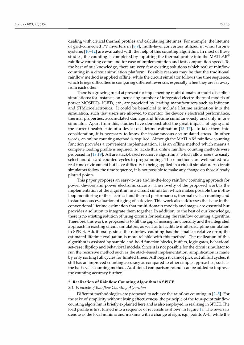
Different methodologies are proposed to achieve the rainflow counting in [2–5]. Forthe sake of simplicity without losing effectiveness, the principle of the four-point rainflowcounting algorithm is briefly explained here and is also employed in realizing in SPICE. Theload profile is first turned into a sequence of reversals as shown in Figure 1a. The reversalsdenote as the local minima and maxima with a change of sign, e.g., points A–L, while the

Energies 2022, 15, 5159 3 of 13

difference between the two reversals is described as range, e.g., r(AB). Then, three adjacentranges are continuously compared to determine the counting action following the criteriathat X2 ≤ X3 and X2 ≤ X1. If satisfied, a closed loop is formed, and the range X2 is countedas a full cycle. Finally, reversals involved in the counted range will be discarded, and a newrange between uncounted reversals will be similarly formed, and the comparisons keepon. For instance, once r(EF) in the loop of D–E–F–G in Figure 1a is counted, both E and Fwill be discarded, and the new range becomes r(DG). By doing so, it is possible to pick outall of the full cycles in the load profile, and only a few uncounted half cycles remain. Insummary, the principle of the four-point algorithm is simple, and since it requires recursiveimplementation, it is a more programming friendly algorithm.

Figure 1. (a) Example of reversal sequence; and (b) four-point rainflow algorithm.

2.2. Implementation Method in SPICE

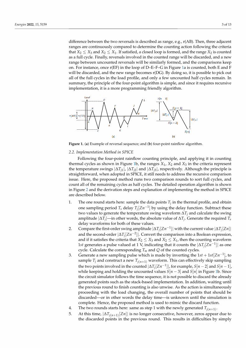
Following the four-point rainflow counting principle, and applying it in countingthermal cycles as shown in Figure 1b, the ranges X1, X2 and X3 in the criteria representthe temperature swings |∆Tj1|, |∆Tj2| and |∆Tj3|, respectively. Although the principle isstraightforward, when adopted in SPICE, it still needs to address the recursive comparisonissue. Here, the proposed method runs two comparison rounds to sort full cycles, andcount all of the remaining cycles as half cycles. The detailed operation algorithm is shownin Figure 2 and the derivation steps and explanation of implementing the method in SPICEare described below.

1. The one round starts here: sample the data points Tj in the thermal profile, and obtainone sampling period Ts delay Tj[Zn−1] by using the delay function. Subtract thesetwo values to generate the temperature swing waveform ∆Tj and calculate the swingamplitude |∆Tj|—in other words, the absolute value of ∆Tj. Generate the required Tsdelay waveforms for both of these values.

2. Compare the first-order swing amplitude |∆Tj[Zn−1]|with the current value |∆Tj[Zn]|and the second-order |∆Tj[Zn−2]|. Convert the comparison into a Boolean expression,and if it satisfies the criteria that X2 ≤ X3 and X2 ≤ X1, then the counting waveform1st generates a pulse valued at 1 V, indicating that it counts the |∆Tj[Zn−1]| as onecycle. Calculate the corresponding Tm and Q of the counted cycles.

3. Generate a new sampling pulse which is made by inverting the 1st + 1st[Zn−1], tosample Tj and construct a new Tj(n+1) waveform. This can effectively skip samplingthe two points involved in the counted |∆Tj[Zn−1]|, for example, S[n− 2] and S[n− 1],while keeping and holding the uncounted values S[n− 3] and S[n] in Figure 1b. Sincethe circuit simulator follows the time sequence, it is not possible to discard the alreadygenerated points such as the stack-based implementation. In addition, waiting untilthe previous round to finish counting is also unwise. As the action is simultaneouslyproceeding with the load changing, the overall number of points that should bediscarded—or in other words the delay time—is unknown until the simulation iscomplete. Hence, the proposed method is used to mimic the discard function.

4. The two rounds starts here: same as step 1 with the newly generated Tj(n+1).5. At this time, |∆Tj(n+1)[Zn]| is no longer consecutive, however, zeros appear due to

the discarded points in the previous round. This results in difficulties by simply

Energies 2022, 15, 5159 4 of 13

adopting the same method as in step 2. Thus, another solution is given here. Deter-mine the growing trend of the temperature swing by comparing |∆Tj(n+1)[Zn]| with|∆Tj(n+1)[Zn−1]|. A falling trend is indicated if the current |∆Tj(n+1)[Zn]| is smalleror equal to |∆Tj(n+1)[Zn−1]|. Otherwise, it is following a rising trend. Based on thecriteria that X2 ≤ X3 and X2 ≤ X1, X2 must have the smallest range. Thus, fullcycles at the end of falling segments will always exist, just next to the following risingsegment. As the one round discards even numbers of points, for instance, two pointsfor 1 counted cycle, four points for two consecutive counted cycles, etc., the full cyclesare most likely to occur in odd delay times, e.g., [Zn−1/−3/−5]. Therefore, the solutionis to pick out full cycles by shifting the |∆Tj(n+1)| five times, from [Zn−1] to [Zn−5], todetermine the first cycle that overlaps with the rising segment. Within five Ts periods,it is capable of filtering out most of the full cycles in this round.

6. Unify the counted cycles to the same delay times [Zn−5] and calculate their sum.Same as step 3 and generate with a new sampling pulse made by inverting theaforementioned pulses, and output a new Tj(n+2) waveform.

7. The three rounds starts here: same as step 1 with the newly generated Tj(n+2).8. Same as step 2, and the loop stops here. The remaining ∆Tj(n+2) values are counted

as half cycles. Calculate the corresponding Tm and Q of half cycles.

Figure 2. Operation of the proposed rainflow counting algorithm in LTspice®.

In summary, the proposed implementation of rainflow counting continuously com-pares the values of three adjacent temperature swings |∆Tjn(n=1,2,3)| for the first two rounds.Counting pulses will be generated during the comparison, and its inverted waveform willbe used as the sampling pulse for producing the next round Tj(n+1)(n=1,2). By doing so, thecounted points can be skipped sampling, and the next round Tj(n+1)(n=1,2) waveforms aresimplified. The remaining cycles in the round 3 are all counted as half cycles.

It should be noted that two rounds cannot filter out all full cycles. In fact, in theory, itrequires numerous rounds to achieve it. However, the difficulty, complexity and simulationtime of running this are expected to increase rapidly. Hence, the proposed method will

Energies 2022, 15, 5159 5 of 13

inevitably have small errors. Nevertheless, it is possible to modularize the two-roundoperation and add it as an additional round to improve the counting accuracy. As a trade-off, the simulation time will be increased. For illustration purposes, this paper only explainsthe three key steps of the proposed rainflow counting. The detailed implementation of thisalgorithm in a circuit simulator will be introduced in the following section.

2.3. Circuitry Analysis

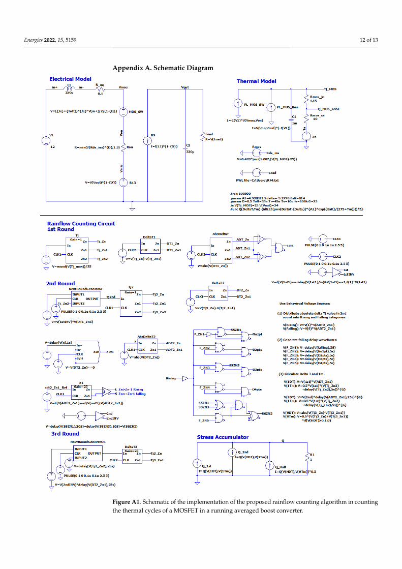
The implementation of the algorithm is carried out in LTspice®, which is a user-friendlyand free circuit simulator. In order to verify the effectiveness of the proposed model, it isapplied to estimate the lifetime of the MOSFET in a free-running boost converter accordingto random load-profiles. The complete circuity of the proposed counting method and theelectro-thermal averaged boost converter model are shown in Figure A1 in Appendix A.Since LTspice® focuses on electrical domain simulation, the temperature (◦C) and powerloss (W) in the thermal domain are modeled by behavioral voltage (V) and current (A)sources in the electrical domain, respectively.

2.3.1. Electro-Thermal Averaged Model

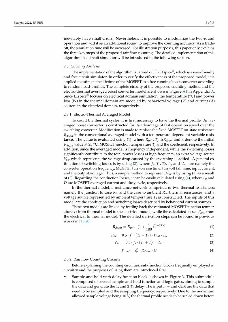
To count the thermal cycles, it is first necessary to have the thermal profile. An av-eraged boost converter is constructed for its advantage of fast operation speed over theswitching converter. Modification is made to replace the fixed MOSFET on-state resistanceRds,on in the conventional averaged model with a temperature-dependent variable resis-tance. The value is evaluated using (1), where Rinit, Tj, ∆Rds,on and α denote the initialRds,on value at 25 ◦C, MOSFET junction temperature Tj and the coefficient, respectively. Inaddition, since the averaged model is frequency independent, while the switching lossessignificantly contribute to the total power losses at high frequency, an extra voltage sourceVsw which represents the voltage drop caused by the switching is added. A general es-timation of switching losses is by using (2), where fs, Tr, Tf , Iin and Vout are namely theconverter operation frequency, MOSFET turn-on rise time, turn-off fall time, input current,and the output voltage. Thus, a simple method to represent Vsw is by using (3) as a resultof (2). Regarding the conduction losses, it can be easily calculated using (4), where im andD are MOSFET averaged current and duty cycle, respectively.

In the thermal model, a resistance network comprised of two thermal resistances:namely the junction to case Rjc and the case to ambient Rca thermal resistances, and avoltage source represented by ambient temperature Ta is constructed. The inputs of thismodel are the conduction and switching losses described by behavioral current sources.

These two models are linked by feeding back the estimated MOSFET junction temper-ature Tj from thermal model to the electrical model, while the calculated losses Ploss fromthe electrical to thermal model. The detailed derivation steps can be found in previousworks in [15,20].

Rds,on = Rinit · (1 +α

100)Tj−25◦C (1)

Psw = 0.5 · fs · (Tr + Tf ) ·Vout · Iin (2)

Vsw = 0.5 · fs · (Tr + Tf ) ·Vout (3)

Pcond = i2m · Rds,on · D (4)

2.3.2. Rainflow Counting Circuits

Before explaining the counting circuities, sub-function blocks frequently employed incircuitry and the purposes of using them are introduced first.

• Sample-and-hold with delay function block is shown in Figure 3. This submoduleis composed of several sample-and-hold function and logic gates, aiming to samplethe data and generate the 1, and 2 Ts delay. The input in+ and CLK are the data thatneed to be sampled and the sampling frequency, respectively. Due to the maximumallowed sample voltage being 10 V, the thermal profile needs to be scaled down before

Energies 2022, 15, 5159 6 of 13

being input to this function. It can be converted back to its original value by using avoltage-dependent voltage source E to provide a gain. The pre-defined value is 1.

• Behavioral Schmitt-triggered buffer with differential inputs is utilized in comparingthe input amplitudes, and outputs a Boolean result.

• Logic gates including AND, NOT and OR gates are used in making decisions if a cycleshould be counted or not.

• Behavioral models, which include behavioral current or voltage sources, allow theuser to define the required functions. A few functions employed in this algorithm andalso in the electrical circuits are explained in Table 1, and further description can befound in [21].

• Next round Tj(n+1) waveform generator, as shown in Figure 4, where input 1, input2 and CLK are the uncounted ∆Tj(n), Tj(n) and sampling pulse, respectively, whilethe output is the Tj(n+1) waveform. After sampling the ∆Tj(n) values, it will be splitinto two groups which contain pure positive and negative values, respectively. Usingthe behavioral set–reset flipflop, the positive pulse can be extended until it meetsthe negative value, and vice versa. By doing so, the uncounted Tj(n) will be keptand extended until meeting the next uncounted value. The achievement of the nextround waveform is by adding the positive and negative outputs together through anIF function.

Figure 3. Sample-and-hold with delay function block: (a) symbol of the block with 1 Ts delay;(b) symbol of the block with two-order delay; and (c) schematic of (b).

Figure 4. Next round Tj(n+1) waveform generator: (a) symbol; and (b) schematic.

Energies 2022, 15, 5159 7 of 13

Table 1. Description and explanation of LTspice®.functions used in the proposed model.

Function Description [21]Purposes of These

Functions in the Model

if(x,y,z) If x is true, do y else z Conditional statement

idt(x) Integrate x Accumulate stresses Q

delay(x,t) x delayed by t

Generate a waveformwith t cycles delayed

for comparison

abs(x) Absolute value of x Calculate amplitude ∆Tj

uramp(x) If x > 0 , output x, else 0Split positive and

negative ∆Tj

As can be seen from the rainflow counting circuits in Figure A1, the counting step inone round is simple. It only contains sampling Tj, calculating the temperature swing andits amplitude, and generating their delays waveforms by employing sample-and-hold withdelay function blocks and behavioral voltage sources. The determination of a full cycleis by using the behavioral Schmitt-triggered buffer with differential inputs. Since it canonly output the true value when the positive side is larger than the negative side, hence, aninverting comparison is made to achieve the X2 ≤ X3 and X2 ≤ X1 criteria.

Using two rounds is slightly complicated as zeros appear in |∆Tj2|, as explainedin Section 2.2 step (5). A reference waveform |∆T′j2[Zn−1]| is generated to facilitate thecomparison between two non-zero adjacent values, as they may possibly become separatedand far away from each other in the original |∆Tj2|. The reference waveform is firstlyachieved by detecting all zeros in |∆Tj2|, and utilized it as the sampling pulse to samplethe |∆Tj2| again. By doing so, a new waveform, which samples the previous value of allzeros in |∆Tj2| are constructed. This action will result in 1 Ts delay from the |∆Tj2|. Hence,to sum the |∆Tj2[Zn−1]| and the aforementioned pulses together, the reference waveform|∆T′j2[Zn−1]| is formed. For instance, the original |∆Tj2[Zn−1]| is [X3 X2 0 0 X1], while

in reference |∆T′j2[Zn−1]|, it becomes [X3 X2 X2 X2 X1]. With the help of the referencewaveform, the falling and rising cycles can be distinguished.

Shifting the falling cycles V(falling) by one Ts produces the V(F_ZN1), which is usedto meet the rising cycles five times. After each time, cycles that overlap with the risingsegment are deleted, and a new truncated falling cycles waveform will be generated andemployed in the next shifting step. Comparisons are mainly made in 1, 3 and 5 Ts, to searchthe full cycles that when X2 is 1, 3, 5 Ts away from X1, indicating cases that, no cycles, onecycle, and two consecutive cycles are counted between X2 and X1 in a previous round,respectively. Since one counted cycle contains two reversals, discarding them will resultin two zeros in |∆Tj2|. With cycles in even numbers of shifting orders, 2 or 4 Ts will bestraightforwardly deleted as they will either be zeros or cycles X3 before the full cycles X2.

The third round is the simplest one, which counts all of the remaining temperatureswings’ cycles as half cycles. Therefore, only a next-round generator, and a sample-and-hold with delay function block to produce the Tj3 and its one Ts delay Tj3[Zn−1] waveformare required. As they provide enough information for calculating the |∆Tj| and Tm.

The corresponding |∆Tj| and Tm of all cases above are calculated by using (5) and (6),respectively, where C and G indicate the counted cycles of each round, and the gain value,as the temperature is scaled down before inputting into the sample and hold function. Forn and x, they are the corresponding round, and delay Ts.

∆Tj = C · |∆Tj(n)| · G (5)

Tm =12· C · (Tj(n)[Zn−x] + Tj(n)[Zn−x−1]) · G (6)

Energies 2022, 15, 5159 8 of 13

The stress accumulator is utilized to evaluate the accumulated damage of a deviceafter a number of thermal cycles, in other words, the consumed lifetime. It is made byconnecting behavioral current sources in parallel which represent stresses from each round,and injecting them into a 1 ohm resistor to sum the stresses up. To calculate the stressof a device, it is necessary to know two terms, namely the device failure cycles underdifferent operation conditions, and the number of cycles that a device has performed.Widely adopted modified Coffin–Manson model (7) can be used to evaluate the number ofcycles to fail, in which N f , ∆Tj, Tm, Ea, k are the number of cycles before a device gener-ates a fault under certain thermal stress, junction temperature swing, mean temperature,thermal activation energy and Boltzman constant, respectively. Regarding δ and A1, theyare empirical coefficients. The MOSFET model under estimation is the IRFP340, and thecoefficient δ and A1 are −5.2776 and 4.9283× 1013, respectively, given in [22]. The accu-mulated stress Q is determined by Miner’s rule (8), which is a commonly used model ofdescribing fatigue-related failures. The rule evaluates the stress that a device undergoesafter a number of thermal cycles. In the equation, Ni indicates the number of cycles that adevice has performed and N f indicates the corresponding number of cycles to fail undercertain stress. The Q is continuously accumulated, and once it reaches one, its reaches itsthreshold of the end of its useful lifetime.

N f = ∆Tδj A1e

EakTm (7)

Q =n

∑i=1

NiN f

(8)

3. Simulation Results3.1. Simulation Waveform

The simulation results of applying the proposed method to a DC/DC boost converterwith a 700 s (s) random load are given in Figures 5–7 as an illustrative example. The loadV(load) changes every 5 s, and only contains reversal points. The V(tj_mos) and V(rds_ins),namely the simulated MOSFET junction temperature Tj, and the instantaneous Rds,on, sharethe same varying trend. As they follow the (1) that high operation temperature will result ahigh on-state resistance, and it in turn will cause heavy power losses. V(tj_zn), V(tj2_zn),and V(tj3_zn) are the sampled waveforms of V(tj_mos), and the generated 2 and 3 roundsTj after skipping sampling counted points. As V(tj_zn) and V(tj2_zn) will be used in thenext round sample-and-hold function, the gain is 1 for simplicity. The true value needs tobe multiplied by a gain of 25. A fairly clear observation on the simplification of the latterround as compared to the previous one can be found.

Key waveforms utilized in 1 and 2 rounds are shown in Figure 6 to better explainthe counting actions. V(tj_zn), V(adt_zn1) and V(1st) indicate the 1 round sampled Tj, theabsolute value of the temperature swing |∆Tj(n+1)[Zn−1]| and the counting waveform. It iseasy for this round to determine the full cycles due to its ease of comparison. The countedcycles can either appear at the middle value X2, which corresponds to the |∆Tj(n+1)[Zn−1]|,or alternatively, at the third point X3, which is |∆Tj(n+1)[Zn]|. To facilitate the later stresscalculation, the second point corresponding waveform is always selected.

While with two round, V(adt2_zn1) and V(adt2_zn1_ref) are the |∆Tj2[Zn−1]|, and itscorresponding reference waveform |∆Tj2′ [Zn−1]|. With the help of reference waveform,|∆Tj2[Zn−1]| can be divided into two groups, namely V(falling) and V(rising) with cyclesonly in a declining/increasing in it. The V(2nd) displays all of the counted cycles in tworounds, with 5 Ts delay time away from the |∆Tj2[Zn−1]|.

Energies 2022, 15, 5159 9 of 13

Figure 5. Waveforms of the proposed method of running a 700 s randomly generated load as anillustrative example.

Figure 6. Example waveforms of depicting the counting actions of the 1 and 2 rounds for explanation.

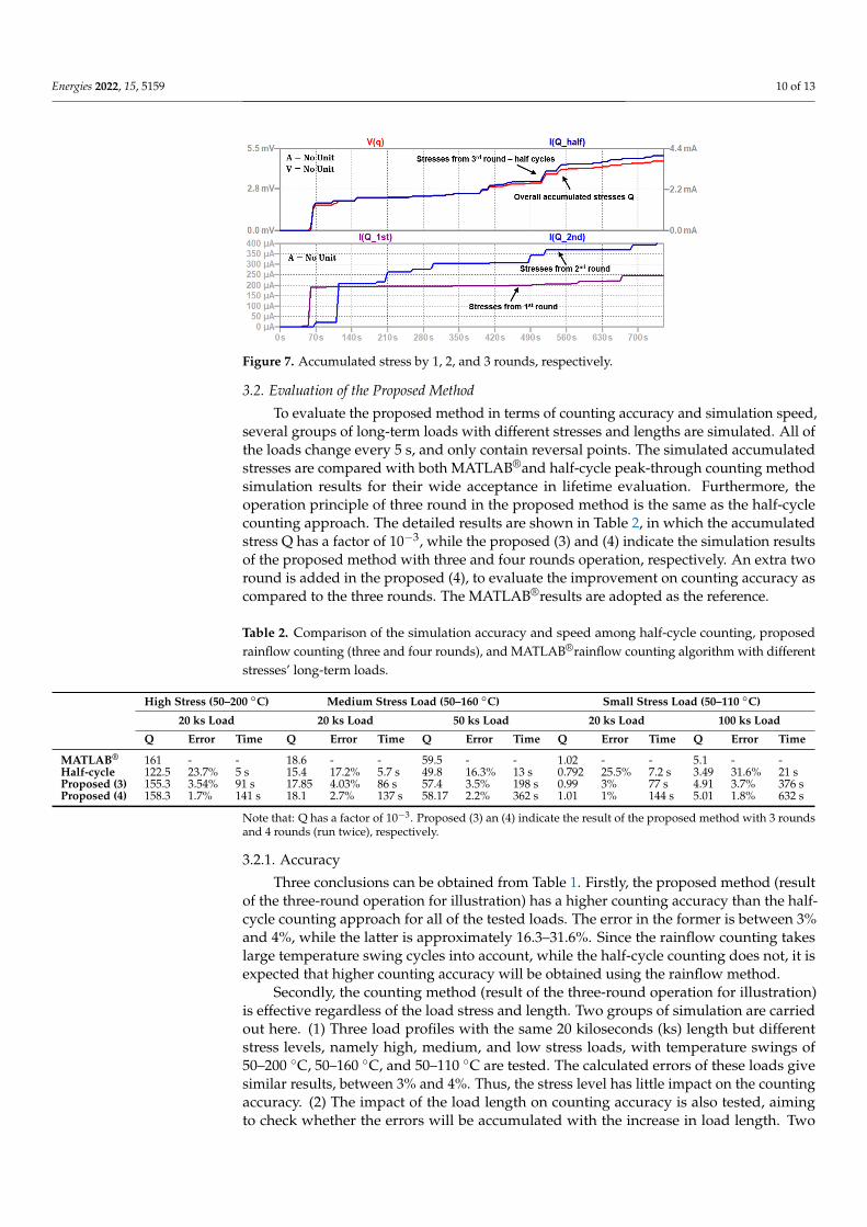
Stress accumulation performance is shown in Figure 7. Since the proposed rainflowcounting is an online method, a continuous accumulation of stresses from one, two andthree rounds with the simulation can be seen. Both steep and flat increases occur in all ofthe stresses. In addition, the stresses from half cycles take the highest portion in the overallaccumulated one. The reason of these can be found from (7), where the ∆Tj is the dominantterm. Hence, the steepness is highly dependent on the temperature swing ∆Tj. As the firstand second round filtered out small full cycles while the large ∆Tj cycles are left, the halfcycles contribute the most.

Energies 2022, 15, 5159 10 of 13

Figure 7. Accumulated stress by 1, 2, and 3 rounds, respectively.

3.2. Evaluation of the Proposed Method

To evaluate the proposed method in terms of counting accuracy and simulation speed,several groups of long-term loads with different stresses and lengths are simulated. All ofthe loads change every 5 s, and only contain reversal points. The simulated accumulatedstresses are compared with both MATLAB®and half-cycle peak-through counting methodsimulation results for their wide acceptance in lifetime evaluation. Furthermore, theoperation principle of three round in the proposed method is the same as the half-cyclecounting approach. The detailed results are shown in Table 2, in which the accumulatedstress Q has a factor of 10−3, while the proposed (3) and (4) indicate the simulation resultsof the proposed method with three and four rounds operation, respectively. An extra tworound is added in the proposed (4), to evaluate the improvement on counting accuracy ascompared to the three rounds. The MATLAB®results are adopted as the reference.

Table 2. Comparison of the simulation accuracy and speed among half-cycle counting, proposedrainflow counting (three and four rounds), and MATLAB®rainflow counting algorithm with differentstresses’ long-term loads.

High Stress (50–200 ◦C) Medium Stress Load (50–160 ◦C) Small Stress Load (50–110 ◦C)

20 ks Load 20 ks Load 50 ks Load 20 ks Load 100 ks Load

Q Error Time Q Error Time Q Error Time Q Error Time Q Error Time

MATLAB® 161 - - 18.6 - - 59.5 - - 1.02 - - 5.1 - -Half-cycle 122.5 23.7% 5 s 15.4 17.2% 5.7 s 49.8 16.3% 13 s 0.792 25.5% 7.2 s 3.49 31.6% 21 sProposed (3) 155.3 3.54% 91 s 17.85 4.03% 86 s 57.4 3.5% 198 s 0.99 3% 77 s 4.91 3.7% 376 sProposed (4) 158.3 1.7% 141 s 18.1 2.7% 137 s 58.17 2.2% 362 s 1.01 1% 144 s 5.01 1.8% 632 s

Note that: Q has a factor of 10−3. Proposed (3) an (4) indicate the result of the proposed method with 3 roundsand 4 rounds (run twice), respectively.

3.2.1. Accuracy

Three conclusions can be obtained from Table 1. Firstly, the proposed method (resultof the three-round operation for illustration) has a higher counting accuracy than the half-cycle counting approach for all of the tested loads. The error in the former is between 3%and 4%, while the latter is approximately 16.3–31.6%. Since the rainflow counting takeslarge temperature swing cycles into account, while the half-cycle counting does not, it isexpected that higher counting accuracy will be obtained using the rainflow method.

Secondly, the counting method (result of the three-round operation for illustration)is effective regardless of the load stress and length. Two groups of simulation are carriedout here. (1) Three load profiles with the same 20 kiloseconds (ks) length but differentstress levels, namely high, medium, and low stress loads, with temperature swings of50–200 ◦C, 50–160 ◦C, and 50–110 ◦C are tested. The calculated errors of these loads givesimilar results, between 3% and 4%. Thus, the stress level has little impact on the countingaccuracy. (2) The impact of the load length on counting accuracy is also tested, aimingto check whether the errors will be accumulated with the increase in load length. Two

Energies 2022, 15, 5159 11 of 13

cases are tested here: (a) Medium stress load profiles with 20 ks and 50 ks; and (b) Smallstress load profiles with 20 ks and 100 ks length are simulated, respectively. No significantaccumulation of errors can be observed. Hence, the counting accuracy is independent ofthe load length.

Thirdly, it can also be observed that adding an extra round can effectively improve theaccuracy by 1.3–2% further, generally from 3 to 4% in three rounds to 1–3%.

3.2.2. Simulation Time

The simulation is carried out on a laptop computer, with Inter(R) Core(TM) i7-7600UCPU. The reported elapse time of running the half-cycle algorithm with these 20–100 ksloads is between 5 s and 21 s, while for the proposed (3), it is between 77 s and 367 s.The half cycle counting has the advantage of its fast simulation speed, as it does notrequire any comparison; hence, less circuitries are used. For the proposed method, as thetrade-off for the improved accuracy, the simulation speed is scarified as compared to thehalf-cycle counting method. Moreover, an increase of more than 50% in simulation timecan be achieved by adding an additional round in proposed (4). Nevertheless, given thel00 ks load profile with 20,000 points and finishing both electro-thermal modeling andthermal cycles counting within less than 7 min is not unacceptable. A high performancecomputational system can also be used if a high speed is required. Since the MATLAB®

rainflow counting is offline, its operation speed is not considered here.

4. Conclusions

This paper presents a circuit-based rainflow counting algorithm in device lifetimeestimation application, aiming to achieve in-the-loop and high accuracy counting, whilstrealizing multi-domain simulation in a circuit simulator. The proposed method followsthe principle of the four-point rainflow counting algorithm, which continuously comparesadjacent temperature swings in a thermal profile to figure out full cycles for two rounds.Counting pulses will be generated during the comparison, and its inverse will be used asthe sampling pulse for producing a simplified thermal profile Tj(n+1) for the next round,where counted reversals are discarded. The remaining cycles will be counted as half cycles.To verify the performance of the proposed method, it is applied to estimate the lifetime ofan operating MOSFET in a boost converter. The simulated accumulated stress is comparedwith the MATLAB® simulation results and also with the half-cycle peak-through countingmethod. Results show that the proposed method has an improved counting accuracy with3–4% errors as compared to the half-cycle counting method which is 16.3–31.6% underdifferent load conditions. It is also reported that a further refinement of the accuracy of1.3–2% can be achieved by adding an extra comparison round. Simulation speed willbe inevitably increased as a trade-off for the enhanced counting accuracy. Nevertheless,with 100 ks, the load profile finished simulating in less than 7 min is still acceptable. Ahigh-speed computing system can also be utilized to compensate this effect if the simulationspeed is a requirement.

Author Contributions: Conceptualization, methodology, software, validation and writing—originaldraft preparation, T.C.; writing—review and editing, D.D.-C.L. and Y.P.S.; supervision, D.D.-C.L. andY.P.S. All authors have read and agreed to the published version of the manuscript.

Funding: This research received no external funding.

Institutional Review Board Statement: Not applicable.

Informed Consent Statement: Not applicable.

Conflicts of Interest: The authors declare no conflict of interest.

Energies 2022, 15, 5159 12 of 13

Appendix A. Schematic Diagram

Figure A1. Schematic of the implementation of the proposed rainflow counting algorithm in countingthe thermal cycles of a MOSFET in a running averaged boost converter.

Energies 2022, 15, 5159 13 of 13

References1. Ciappa, M.; Carbognani, F.; Fichtner, W. Lifetime prediction and design of reliability tests for high-power devices in automotive

applications. IEEE Trans. Device Mater. Rel. 2003, 3, 191–196.2. ASTM E1049-85; Standard Practices for Cycle Counting in Fatigue Analysis. ASTM: West Conshohocken, PA, USA, 2011.3. Application Notes AN2019-05-“PC and TC Diagrams”; Infineon Technologies: Neubiberg, Germany, 2019.4. Matlab, Rainflow Counts for Fatigue Analysis. Available online: https://au.mathworks.com/help/signal/ref/rainflow.html

(accessed on 14 June 2022).5. McInnes, C.H.; Meehan, P.A. Equivalence of four-point and three-point rainflow cycle counting algorithms. Int. J. Fatigue 2008, 30,

547–559.6. Mainka, K.; Thoben, M.; Schilling, O. Lifetime calculation for power modules application and theory of models and counting

methods. In Proceedings of the 2011 14th European Conference on Power Electronics and Applications, Birmingham, UK,30 August–1 September 2011; pp. 1–8.

7. Matsuishi, M.; Endo, T. Fatigue of metals subjected to varying stress. Jpn. Soc. Mech. Eng. 1968, 68, 37–40.8. Sangwongwanich, A.; Yang, Y.; Sera, D.; Blaabjerg, F. Lifetime Evaluation of Grid-Connected PV Inverters Considering Panel

Degradation Rates and Installation Sites. IEEE Trans. Power Electron. 2018, 33, 1225–1236.9. Shen, Y.; Chub, A.; Wang, H.; Vinnikov, D.; Liivik, E.; Blaabjerg, F. Wear-Out Failure Analysis of an Impedance-Source PV

Microinverter Based on System-Level Electrothermal Modeling. IEEE Trans. Ind. Power Electron. 2019, 66, 3914–3927.10. Shipurkar, U.; Lyrakis, E.; Ma, K.; Polinder, H.; Ferreira, J.A. Lifetime Comparison of Power Semiconductors in Three-Level

Converters for 10-MW Wind Turbine Systems. IEEE J. Emerg. Sel. Top. Power Electron. 2018, 6, 1366–1377.11. Liu, H.; Ma, K.; Qin, Z.; Loh, P.C.; Blaabjerg, F. Lifetime Estimation of MMC for Offshore Wind Power HVDC Application. IEEE J.

Emerg. Sel. Top. Power Electron. 2016, 4, 504–511.12. Ma, K.; Liserre, M.; Blaabjerg, F.; Kerekes, T. Thermal Loading and Lifetime Estimation for Power Device Considering Mission

Profiles in Wind Power Converter. IEEE Trans. Power Electron. 2015, 30, 590–602.13. Huang, H.; Mawby, P.A. A Lifetime Estimation Technique for Voltage Source Inverters. IEEE Trans. Power Electron. 2013, 28,

4113–4119.14. Sintamarean, N.; Blaabjerg, F.; Wang, H.; Iannuzzo, F.; de Place Rimmen, P. Reliability Oriented Design Tool For the New

Generation of Grid Connected PV-Inverters. IEEE Trans. Power Electron. 2015, 30, 2635–2644.15. Cheng, T.; Lu, D.D.C.; Siwakoti, Y.P. A MOSFET SPICE Model With Integrated Electro-Thermal Averaged Modeling, Aging, and

Lifetime Estimation. IEEE Access 2021, 9, 5545–5554.16. Lai, W.; Chen, M.; Ran, L.; Xu, S.; Jiang, N.; Wang, X.; Alatise, O.; Mawby, P. Experimental Investigation on the Effects of Narrow

Junction Temperature Cycles on Die-Attach Solder Layer in an IGBT Module. IEEE Trans. Power Electron. 2017, 32, 1431–1441.17. Lai, W.; Chen, M.; Ran, L.; Alatise, O.; Xu, S.; Mawby, P. Low ∆Tj Stress Cycle Effect in IGBT Power Module Die-Attach Lifetime

Modeling. IEEE Trans. Power Electron. 2016, 31, 6575–6585.18. Musallam, M.; Johnson, C.M. An Efficient Implementation of the Rainflow Counting Algorithm for Life Consumption Estimation.

IEEE Trans. Reliab. 2012, 61, 978–986.19. Chen, Z.; Gao, F.; Yang, C.; Peng, T.; Zhou, L.; Yang, C. Converter Lifetime Modeling Based on Online Rainflow Counting

Algorithm. In Proceedings of the 2019 IEEE 28th International Symposium on Industrial Electronics (ISIE), Vancouver, BC,Canada, 12–14 June 2019; pp. 1743–1748.

20. Cheng, T.; Lu, D.D.C.; Siwakoti, Y.P. Electro-Thermal Average Modeling of a Boost Converter Considering Device Self-heating.In Proceedings of the 2020 IEEE Applied Power Electronics Conference and Exposition (APEC), New Orleans, LA, USA, 15–19March 2020; pp. 2854-2859.

21. LTspice®B Sources (Complete Reference). Available online: http://ltwiki.org/index.php?title=B_sources_(complete_reference)(accessed on 14 June 2022).

22. Dusmez, S.; Duran, H.; Akin, B. Remaining Useful Lifetime Estimation for Thermally Stressed Power MOSFETs Based on on-StateResistance Variation. IEEE Trans. Ind. Appl. 2016, 52, 2554–2563.