


Bahasa
Halaman
Hukum


Proceedings of 2013 IAHR Congress © 2013 Tsinghua University Press, Beijing
ABSTRACT: With the aim of optimising contact tank design through numerical model simulations,
results are presented herein of an experimental and computational fluid dynamics (CFD) study in a scaled
laboratory model. Three-dimensional numerical simulations of flow and transport characteristics were
conducted using a Reynolds Averaged Navier-Stokes equation approach. Experimental results were
obtained through Acoustic Doppler Velocimetry measurements and a series of conservative tracer
experiments. Focus is given on turbulent structures and undesirable flow patterns that lead to a reduced
disinfection efficiency, through phenomena such as short circuiting and recirculation zones. The
laboratory data analysis indicates extensive three-dimensionality as a result of the current inlet geometry
with a confirmed negative impact on the disinfection performance of the contact tank model, as
demonstrated by Residence Time Distribution curves. Disinfection performance is evaluated through
hydraulic efficiency indicators commonly used in the industry to monitor field-scale disinfection facilities.
Correlations between CFD and experimental data confirm the adequate reproduction of hydrodynamic
conditions and reinforce the predictive capabilities of numerical models as tools to simulate field scale
tanks or optimize existing designs.
KEY WORDS: Contact Tanks, Acoustic Doppler Velocimetry, Tracer Experimentation, RANS,
Disinfection Performance
1 INTRODUCTION
Serpentine contact tank units suggest plug flow to be the ideal hydrodynamic condition at which
disinfection performance is maximized (Falconer and Tebbutt, 1986; Markse and Boyle, 1973). Under
such flow conditions, disinfectant transport becomes ideal by remaining in the tank for a uniform time
interval whilst achieving the desired disinfection. However, previous studies (e.g. Teixeira, 1993) indicate
that flow exhibits a residence time distribution (RTD) which can be significantly different from what is
dictated by plug flow. The shape of the tracer RTD curves can provide an insight into the hydrodynamic
and mixing conditions, as explained by Levenspiel (1999). For example, the residence time at 10%
cumulative RTD constitutes a crucial indicator (t10) for the evaluation of disinfection efficiency and
design suitability at water treatment works. Digression from plug flow can be attributed to the complex
hydrodynamics, namely short-circuiting and recirculation zone formation (Kim et al., 2010).
Short-circuiting occurs when particles pass through a reactor quicker than the theoretical hydraulic
residence time. Recirculation zones not only promote short-circuiting (since they occupy a considerable
part of the tank volume) but they also trap solutes and particles (or pathogens), which are then retained in
the tank for a longer period than the theoretical hydraulic residence time. The occurrence of such flow
patterns has a detrimental effect on the overall efficiency, because contact times of pathogens with the
CFD Study of Flow and Transport Characteristics in Baffled
Disinfection Tanks
Athanasios Angeloudis
Research Student, School of Engineering, Cardiff University, Cardiff CF24 3AA, UK, Email:
Thorsten Stoesser
Professor, School of Engineering, Cardiff University, Cardiff CF24 3AA, UK. Email: [email protected]
Dongjin Kim
Research Assosiate, School of Civil and Environmental Engineering ,Georgia Institute of Technology ,
Atlanta, GA 30332,USA. E-mail: [email protected]
Roger Alexander Falconer
Professor, School of Engineering, Cardiff University, Cardiff CF24 3AA, UK. Email:

2
disinfectant are either too short (insufficient treatment) or too long, which can cause disinfection
by-products.
Computational Fluid Dynamics (CFD) techniques have been implemented widely to simulate flow
conditions and mixing processes during disinfection tank operation (e.g. Kim et al., 2010; Khan et al.,
2006; Wang and Falconer, 1998). Even though the performance of computational models has vastly
improved, there is still concern with regards to the accuracy and ability of numerical models to predict the
turbulence characteristics as well as the actual shape of RTD curves. For reliable simulation results, CFD
models require validation by comparisons against experimental data. However, the availability of such
data in water treatment facilities through in situ experimentation is scarce or limited to “black-box” type
tracer injections due to difficulties in obtaining hydrodynamic or solute transport measurements inside
field scale tanks.
Results are presented herein of an experimental and CFD study in a scaled baffled tank laboratory
model. 3D numerical simulations of flow and tracer transport characteristics were conducted using a
Reynolds Averaged Navier-Stokes (RANS) equation approach. Experimental results were obtained
through ADV measurements and a series of conservative tracer experiments in a scaled baffled contact
tank model in Cardiff University. In this study, tracer monitor points are not only limited at the outlet
section of the tank but are spread out across the geometry for a more thorough overview of mixing
processes. Core objectives of this study were to: (a) inform modelling practises by presenting
hydrodynamic and tracer transport results from a physical model, (b) compare hydrodynamic and solute
transport simulations with available laboratory data so as to examine the validity and potential of the 3D
simulations, and (c) discuss the potential of refining and tailoring CFD models to be used as tool for the
design and retrofitting of water disinfection infrastructure.
Figure 1 (a) Schematic view of laboratory model tank configuration including vectors indicating main streamwise flow direction ; (b) channel inlet and compartment 1 cross-section (dimensions in mm). Experimental data availability is illustrated in both sketches.
2 METHODOLOGY
2.1 Laboratory Model Setup and Experimental Data
Experimental data was acquired from a scaled disinfection tank, which exhibits standard features of
a baffled contact tank, i.e. it is separated into a certain number of compartments where the flow meanders
due to the baffles being arranged in an alternating fashion. The model (denoted as CT-1 in this study) is Lt
= 3.0 m long, Wt = 2.0 m wide and Zt = 1.2 m deep. Internal baffles, 12 mm thick, divide the tank into 8
compartments of Wc = 0.365 m width. The inlet is located in the northeast corner of the tank and consists
of an open channel of width Wc and depth Hi of 0.30 m, which is approximately 1/4 of the tank depth.
Honeycombs located in the approach channel promote uniformity when the flow enters the system. The
water level, controlled via a rectangular sharp crested weir at the outlet, was measured to be at Ht = 1.02
m. A constant flow rate of 4.72 l/s was set when collecting velocity measurements corresponding to a bulk

3
velocity Ub of 12.5 mm/s and a tank theoretical retention time (T=V/Q) of 1265 s. Hydrodynamic
measurements were collected via a 3D ADV technique manufactured by Nortek AS yielding a total of
3200. Pulse tracer experiments involved Rhodamine WT injections at the inlet, while Cyclops-7
submersible sensors monitored fluorescence levels for a sufficient duration (10,000s) at designated
locations. Sensitivity analysis and Instrument Calibration tests were performed prior to any
experimentation to ensure the validity of the measurements. Figure 1 illustrates the laboratory model’s
main geometric features and also depicts velocity measurement and tracer sampling locations. The data
set of the experimental results is denoted here as CT-EXP.
2.2 Numerical Methods and Computational Model Setup
The RANS simulations of the hydrodynamics are performed using an in-house code implementing a
finite-volume approach on a structured orthogonal grid. A Semi-Implicit Method for Pressure-Linked
Equations (SIMPLE) is applied to couple the pressure to the velocity field and the standard k-ε turbulence
closure to compute the Reynolds Stresses. The geometry and boundary conditions of the CFD simulations
are chosen in accordance with the laboratory experiment. At the inlet surface, a Dirichlet boundary
condition is applied for velocity and turbulence parameters. Transversal V and vertical W velocity
components are set to zero and a uniform streamwise velocity U is assumed with a magnitude based on
the experimental study flow rate. A Neumann condition with mass conservation is imposed at the outlet
surface for all variables. The water surface is treated as a rigid, frictionless lid with no shear stress. Side
walls, tank bottom and internal baffles are considered smooth to match the low roughness surfaces of the
laboratory model and low Reynolds number wall functions are employed.
Once the steady state flow field is obtained, the transport of a conservative tracer scalar quantity C is
simulated by solving the three-dimensional Reynolds-averaged advection-diffusion equation. The
turbulent Schmidt number is given the standard value of Sc = 0.7 as suggested in Launder (1978). The
low-diffusive and oscillation-free Hybrid Liner/Parabolic Approximation (Zhu, 1991) approximates the
convective term and the central differencing scheme the diffusion term. The implicit Euler scheme is
employed to integrate the equation in time. Tracer transport is based on the values of velocity Ui and
viscosity vt which are obtained from the converged steady-state hydrodynamics simulation. The tracer
injection is simulated at the inlet of the contact tank for 40 time steps of Δt = 0.25 sec in order to
reproduce the injection interval of the experimental study.
The simulation reproducing the experimental results in CT-1, referred to here as CT-S, were
produced using a non-uniform grid of 161×77×42 cells featuring a variable geometrical grid step to
ensure a more refined grid in areas of interest (i.e. near baffles, walls and inlet flow). The mesh was
subject to a convergence analysis to ensure mesh independence for hydrodynamic and tracer transport
results (Angeloudis et al, 2013).
3 RESULTS AND DISCUSSION
3.1 Flow and Tracer Transport Validation
Figure 2 Velocity vectors in the centre-plane of (a) Compartment 1 and (b) Compartment 2. The blue vectors represent CT-S simulation results and the black vectors represent the ADV (CT-EXP) data
The capacity of the numerical models to reproduce accurately hydrodynamics of the experimental

4
study is examined in Figures 2 and 3. From the vector plot in Figure 2(a) it is clear that the first
compartment is dominated by one large recirculation zone and significant two-dimensionality in the
longitudinal plane. This flow pattern is a result of the inlet configuration which causes the flow to enter
the first chamber by means of a high momentum jet. The recirculation zone occupies a region between
0.20< x/Wt < 1.00 and is centered at (0.60, 0.40). The region between 0.00< x/Wt < 0.20 and 0.00< z/Ht <
0.80 is dictated by very low flow velocities and can arguably be classified as either a dead zone or a
slower portion of the larger vertical recirculation. The conditions of compartment 1, result in subsequent
recirculation zones occurring in compartments downstream (Figure 2b) which combined with the
expected recirculation zones around baffle lees demonstrate the complexity of the tank hydrodynamics. In
terms of compliance between experimental and computational results, main hydrodynamic features are
captured accurately (i.e. flow pattern and magnitude). This is more quantitatively demonstrated in Figure
3, from which it can be seen that the simulated magnitudes of streamwise velocity (U) and turbulent
kinetic energy (k) matches closely the experimental data. From the velocity profile in particular, the
presence of reverse flow is dominant in compartments 1 and 2 but diminishes toward the outlet as seen by
the profile in compartment 8 where experimentally and computationally it resembles uniform flow.
Figure 3 Vertical profiles of a) U/Ub and b) k/Ub2 in compartments 1, 2 and 8 as measured experimentally (CT-EXP)
and predicted computationally (CT-S). Positive are considered the velocities that follow the streamwise direction in each compartment.
Figure 4 RTD curves produced for experimental and computational data at (a) Compartment 1 and (b) Compartment 3: experimental RTDs (left), computational RTDs (right).
Figure 4 presents tracer RTD results obtained experimentally (left) and as predicted computationally
(right) for concentration sampling locations in compartments 1 and 3 respectively. The numerically
predicted RTDs are much smoother than the measured ones, the latter exhibiting the unsteadiness of the
flow. Tracer injected at the inlet is clearly transported by means of convection, as shown by the

5
correlation of figures 2a and 4a. The flow in 2a initially appears only in the top layer of the vertical
profile by means of the inlet jet flow. It then appears in the bottom layer (reverse flow), due to the vertical
recirculation zone, and appears in the middle layer even later. This pattern appears to apply for tracer
transport, by observation of concentration peaks in 4a. The concentration fluctuations in compartment 1
suggest unsteadiness in the flow which is not captured by the RANS simulation. However, for
compartment 3 (Figure 4b), as flow becomes more uniform and the initial three-dimensionality caused by
jet mixing diminishes, RANS simulations produce more accurate RTD predictions which consistently
improve towards the outlet. This is particularly interesting as RTDs are determinant for evaluating the
performance of disinfection facilities by deriving Hydraulic Efficiency Indicators (HEI).
Figure 5 Correlation between experimental and computational results through Hydraulic Efficiency Indicator (HEI) prediction: (a) Dispersion Index (σ2), (b) short-circuiting indicator t10 and (c) Morrill Index (Mo)
Figure 5 presents HEI results for each compartment with a view to monitoring hydraulic
performance in each compartment of the tank. The indicator t10, corresponds to the normalized time since
injection for the passage of 10% of the injected tracer mass through the monitoring section and serves as a
measure for severity of short-circuiting. The HEI Mo (Morrill index), defined as Mo = t90/t10, where t90 is
the normalized time since injection for the passage of 90% of injected tracer mass. The dispersion index
σ2, defined σ
2 = σt
2/tg
2 where σt
2 is the variance of the RTD curve and tg is the normalized time to reach
the centroid of the effluent curve (Markse and Boyle, 1973). HEIs Mo and σ2 reflect the amount of
mixing in the disinfection tank. The indicators are classified into “poor”, “compromising”, “acceptable”
and “excellent” in accordance with guidelines of US EPA (AWWA,1991) and Van der Walt (2002).
Overall, numerical model predictions provide a reliable indication of the disinfection performance
demonstrated by the close agreement against measured results. The non-ideal nature of hydrodynamics
and mixing processes in the contact tank is observed inside the tank, where compromising or even poor
performance is encountered at some tracer sampling points. HEIs drawn from compartments 1-2 (marked
grey in the figure) are considered unreliable as the monitor points are inside recirculation zones where
tracer mass reappears multiple times during the sampling duration (due to convection), thus distorting the
accuracy of RTD curves and their corresponding HEIs.
The comparison of experimental and computational results presented herein, indicates the ability of
the current CFD approach to predict flow and solute transport conditions within disinfection tank
facilities. This can be refined to produce design specific parameters (i.e. HEIs) that can either aid in the
performance of a design prior to construction, or the optimization of an existing design through
retrofitting by evaluation of potential improvements computationally.
3.2 Retrofit of Current Geometry
The optimization of the CT-1 design was examined experimentally by Rauen (2005) in an effort to
neutralize the current inlet water jet that results in the dominance of complex flow in compartments 1 and
2. By implementing a cross-baffling configuration (CT-O), the inlet three-dimensionality is constrained to
a lesser extent of the tank volume (Figure 6a). The impact of retrofitting the design was evaluated through
outlet HEIs (Table 1) which suggest superior performance. The available data presented an opportunity to
quantitatively examine and confirm the predictive capabilities of the current CFD approach. A numerical
model of the CT-O design was setup to simulate a tracer experiment similar to the one undertaken by
Rauen. The present simulation HEIs closely matched the measured values as shown by the percentile
6
deviations of 3.6, 0.1 and 1.8% for σ2, t10 and Mo respectively.
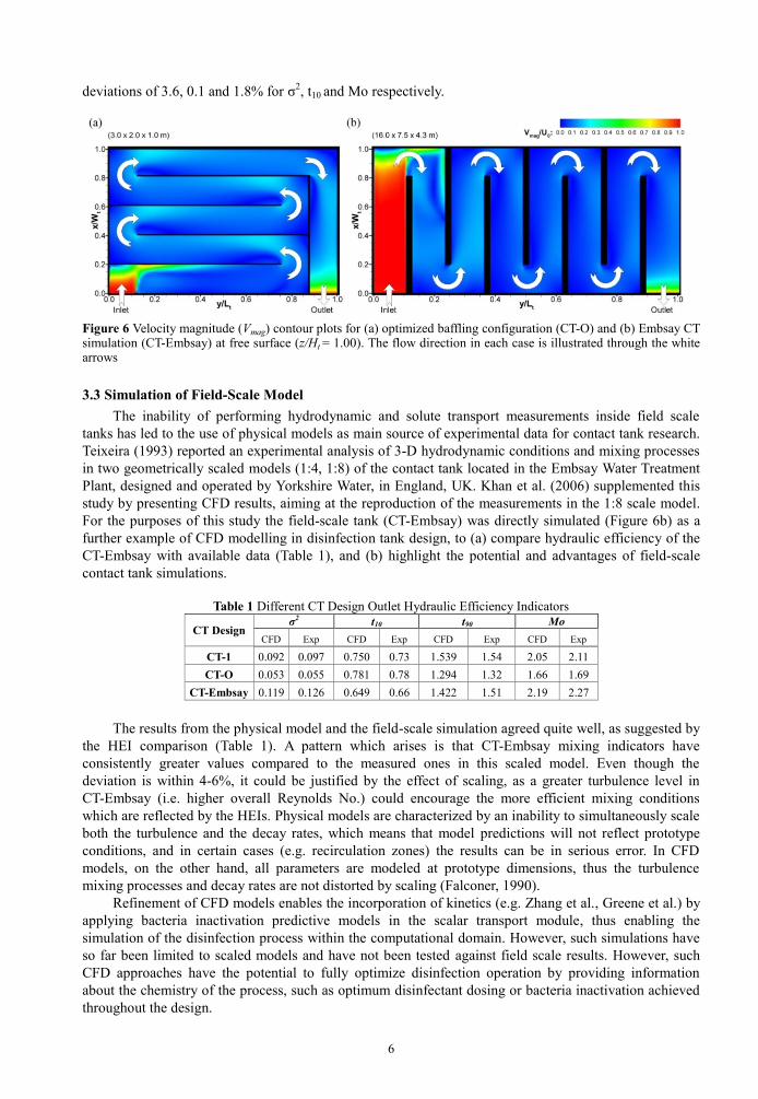
Figure 6 Velocity magnitude (Vmag) contour plots for (a) optimized baffling configuration (CT-O) and (b) Embsay CT simulation (CT-Embsay) at free surface (z/Ht = 1.00). The flow direction in each case is illustrated through the white arrows
3.3 Simulation of Field-Scale Model
The inability of performing hydrodynamic and solute transport measurements inside field scale
tanks has led to the use of physical models as main source of experimental data for contact tank research.
Teixeira (1993) reported an experimental analysis of 3-D hydrodynamic conditions and mixing processes
in two geometrically scaled models (1:4, 1:8) of the contact tank located in the Embsay Water Treatment
Plant, designed and operated by Yorkshire Water, in England, UK. Khan et al. (2006) supplemented this
study by presenting CFD results, aiming at the reproduction of the measurements in the 1:8 scale model.
For the purposes of this study the field-scale tank (CT-Embsay) was directly simulated (Figure 6b) as a
further example of CFD modelling in disinfection tank design, to (a) compare hydraulic efficiency of the
CT-Embsay with available data (Table 1), and (b) highlight the potential and advantages of field-scale
contact tank simulations.
Table 1 Different CT Design Outlet Hydraulic Efficiency Indicators
CT Design σ2 t10 t90 Mo
CFD Exp CFD Exp CFD Exp CFD Exp
CT-1 0.092 0.097 0.750 0.73 1.539 1.54 2.05 2.11
CT-O 0.053 0.055 0.781 0.78 1.294 1.32 1.66 1.69
CT-Embsay 0.119 0.126 0.649 0.66 1.422 1.51 2.19 2.27
The results from the physical model and the field-scale simulation agreed quite well, as suggested by
the HEI comparison (Table 1). A pattern which arises is that CT-Embsay mixing indicators have
consistently greater values compared to the measured ones in this scaled model. Even though the
deviation is within 4-6%, it could be justified by the effect of scaling, as a greater turbulence level in
CT-Embsay (i.e. higher overall Reynolds No.) could encourage the more efficient mixing conditions
which are reflected by the HEIs. Physical models are characterized by an inability to simultaneously scale
both the turbulence and the decay rates, which means that model predictions will not reflect prototype
conditions, and in certain cases (e.g. recirculation zones) the results can be in serious error. In CFD
models, on the other hand, all parameters are modeled at prototype dimensions, thus the turbulence
mixing processes and decay rates are not distorted by scaling (Falconer, 1990).
Refinement of CFD models enables the incorporation of kinetics (e.g. Zhang et al., Greene et al.) by
applying bacteria inactivation predictive models in the scalar transport module, thus enabling the
simulation of the disinfection process within the computational domain. However, such simulations have
so far been limited to scaled models and have not been tested against field scale results. However, such
CFD approaches have the potential to fully optimize disinfection operation by providing information
about the chemistry of the process, such as optimum disinfectant dosing or bacteria inactivation achieved
throughout the design.

7
4 CONCLUSIONS
In this study a RANS based CFD technique was employed to predict flow, transport processes and
hydraulic efficiency in serpentine contact tanks. The CFD model was first validated by comparing
simulated velocity and tracer prediction with experimental data obtained from an Acoustic Doppler
Velocimetry measurement program and conservative tracer experiments in a physical contact tank model.
The analysis was complemented with the evaluation of contact tank performance using disinfection
specific Hydraulic Efficiency Indicators (i.e. t10, σ2 and Mo). These were calculated at various locations
inside the tank rather than only at the outlet, which provided a better understanding of the mixing
processes inside the model and not treat the contact tank operation as a “black box”.
The predictive capabilities of the numerical model were then demonstrated by simulating a
retrofitted design of the laboratory model, reaffirming the implementation of validated CFD approaches
as suitable design tools. The scale of the problem was then expanded by simulating a field-scale tank
highlighting how the computational simulations do not have to be constrained by the uncertainties and
scaling problems leading to the Froude-Reynolds conflict of small-scale physical models. It is shown that
a 3-D CFD model can aide in and/or guide the design of contact tanks by providing reliable predictions of
flows, scalar transport and hydraulic efficiency. There is the need to further refine the model with more
sophisticated kinetic bacteria inactivation models which could more specifically describe disinfection
reactions (i.e. disinfectant decay, pathogen inactivation, by-product formation). Such refinements would
provide even more detailed analyses of newly designed or retrofitted CTs.
ACKNOWLEDGEMENT
The first author acknowledges the financial support of Halcrow, a CH2M Hill company.
References
American Water Works Association (AWWA), 1991. Guidance Manual for compliance with the filtration and disinfection requirements for public water systems using surface water sources, Denver
Angeloudis, A., Stoesser, T., Kim, D. and Falconer, R.A., 2013. Computational Modelling of Flow and Disinfection Processes in Contact Tanks. Water Management – Proceedings of the ICE (in review).
Falconer, R. A., 1990. Engineering Problems and the Application of Mathematical Models Relating to Combating Water Pollution. Municipal Engineer, 7, 281-291.
Falconer, R. A. and Tebbutt, T. H. Y., 1986. A Theoretical and Hydraulic Model Study of a Chlorine Contact Tank. Proceedings of the Institution of Civil Engineers, Part 2-Research and Theory, 81, 255-276.
Khan, L. A., Wicklein E. A. and Teixeira, E. C., 2006. Validation of a Three-Dimensional Computational Fluid Dynamics Model of a Contact Tank. Journal of Hydraulic Engineering 132(7), 741-746.
Kim, D., Kim, D., Kim, J. H. and Stoesser, T., 2010. Large Eddy Simulation of Flow and Tracer Transport in Multichamber Ozone Contactors. Journal of Environmental Engineering, 136(1), 22-31.
Launder, B. E., 1978. Heat and Mass Transport. Turbulence, Chapter 5, P. Bradshaw, ed., Springer, Berlin Levenspiel, O., 1999. Chemical Reaction Engineering. 3rd ed., John Wiley & Sons, New York. Marske, D. M. and Boyle, J. D., 1973. Chlorine Contact Chamber Design – A Field Evaluation. Water and Sewage
Works, 120(1), 70-77. Rauen, W. B., 2005. Physical and Numerical Modelling of 3-D Flow and Mixing Processes in Contact Tanks. PhD
Thesis, Cardiff University. Rauen, W.B., Angeloudis A. and Falconer, R.A., 2012. Appraisal of Chlorine Contact Tank Modelling Practices.
Water Research, 46(18), 5834-5847 Teixeira, E. C., 1993. Hydrodynamic Processes and Hydraulic Efficiency of Chlorine Contact Units. PhD Thesis,
University of Bradford. Van der Walt, J. J., 2002. The Modelling of Water Treatment Process Tanks. PhD Thesis, Rand Afrikaans
University. Wang, H. and Falconer, R. A., 1998. Simulating Disinfection Processes in Chlorine Contact Tanks using Various
Turbulence Models and High-Order Accurate Difference Schemes. Water Research, 32(5), 1529-1543. Zhang, G., Lin, B. and Falconer, R. A., 2000. Modelling Disinfection By-products in Contact Tanks. Journal of
Hydroinformatics, 2(2), 123-132. Zhu, J., 1991. A Low-diffusive and Oscillation-free Convection scheme. Communications in Applied Numerical
Methods, 7, 225-232.
Top Related
Copyright © 2022 FDOKUMEN

