


Bahasa
Halaman
Hukum

Brain-wide mapping of neural activity controlling zebrafish exploratory locomotion
CitationDunn, Timothy W, Yu Mu, Sujatha Narayan, Owen Randlett, Eva A Naumann, Chao-Tsung Yang, Alexander F Schier, Jeremy Freeman, Florian Engert, and Misha B Ahrens. 2016. “Brain-wide mapping of neural activity controlling zebrafish exploratory locomotion.” eLife 5 (1): e12741. doi:10.7554/eLife.12741. http://dx.doi.org/10.7554/eLife.12741.
Published Versiondoi:10.7554/eLife.12741
Permanent linkhttp://nrs.harvard.edu/urn-3:HUL.InstRepos:26860207
Terms of UseThis article was downloaded from Harvard University’s DASH repository, and is made available under the terms and conditions applicable to Other Posted Material, as set forth at http://nrs.harvard.edu/urn-3:HUL.InstRepos:dash.current.terms-of-use#LAA
Share Your StoryThe Harvard community has made this article openly available.Please share how this access benefits you. Submit a story .
Accessibility
*For correspondence: ahrensm@
janelia.hhmi.org
†These authors contributed
equally to this work‡These authors also contributed
equally to this work
Competing interests: The
authors declare that no
competing interests exist.
Funding: See page 26
Received: 03 November 2015
Accepted: 09 March 2016
Published: 22 March 2016
Reviewing editor: Ronald L
Calabrese, Emory University,
United States
Copyright Dunn et al. This
article is distributed under the
terms of the Creative Commons
Attribution License, which
permits unrestricted use and
redistribution provided that the
original author and source are
credited.
Brain-wide mapping of neural activitycontrolling zebrafish exploratorylocomotionTimothy W Dunn1,2,3†, Yu Mu3†, Sujatha Narayan3, Owen Randlett1,Eva A Naumann1,4, Chao-Tsung Yang3, Alexander F Schier1,2, Jeremy Freeman3‡,Florian Engert1,2‡, Misha B Ahrens3*‡
1Department of Molecular and Cellular Biology, Harvard University, Cambridge,United States; 2Program in Neuroscience, Department of Neurobiology, HarvardMedical School, Boston, United States; 3Janelia Research Campus, Howard HughesMedical Institute, Ashburn, United States; 4Department of Neuroscience, Physiologyand Pharmacology, University College London, London, United Kingdom
Abstract In the absence of salient sensory cues to guide behavior, animals must still execute
sequences of motor actions in order to forage and explore. How such successive motor actions are
coordinated to form global locomotion trajectories is unknown. We mapped the structure of larval
zebrafish swim trajectories in homogeneous environments and found that trajectories were
characterized by alternating sequences of repeated turns to the left and to the right. Using whole-
brain light-sheet imaging, we identified activity relating to the behavior in specific neural
populations that we termed the anterior rhombencephalic turning region (ARTR). ARTR
perturbations biased swim direction and reduced the dependence of turn direction on turn history,
indicating that the ARTR is part of a network generating the temporal correlations in turn direction.
We also find suggestive evidence for ARTR mutual inhibition and ARTR projections to premotor
neurons. Finally, simulations suggest the observed turn sequences may underlie efficient
exploration of local environments.
DOI: 10.7554/eLife.12741.001
IntroductionLocomotion trajectories must be highly structured to achieve goals that cannot be reached by indi-
vidual motor actions (Flavell et al., 2013; Berman et al., 2014; Maye et al., 2007). When environ-
mental cues such as odor gradients or visual landmarks are present, these can be used to guide
sequential motor actions in a goal-driven manner, such as navigating up an odor gradient toward
food (Gomez-Marin et al., 2010). When such cues are lacking, however, behavior must be struc-
tured so that efficient foraging and exploration can continue until cues are found. This behavior
often follows optimal algorithms (Stephens, 1986; Charnov, 1976) that must be guided by internal
brain activity. Such internal activity is necessarily embedded in brain-wide patterns of spontaneous
activity, but the relevant signals and brain areas remain elusive.
Decades of motor system research have identified many regions involved in the initiation of loco-
motion. The basal ganglia, which are closely associated with action selection, have been studied
extensively in mammals and more recently in lamprey (Stephenson-Jones et al., 2011), and the
mesencephalic locomotor region (MLR) (Sirota et al., 2000; Dubuc et al., 2008) and the dience-
phalic locomotor region (DLR) (El Manira et al., 1997) are causally linked to coordinated motor out-
put. However, many other regions show activity related to motor patterns (e.g. [Arrenberg et al.,
2009]), and it is possible that many adjunct motor centers have yet to be characterized. In any case,
Dunn et al. eLife 2016;5:e12741. DOI: 10.7554/eLife.12741 1 of 29
RESEARCH ARTICLE
it is likely that multiple circuits participate in shaping the fine structure of motor output. Further-
more, it is unknown how higher level structure in spontaneous behavior, potentially reflecting goal-
driven internal states like those underlying foraging and surveillance, might be realized in circuitry
across the vertebrate brain.
We investigated the spatiotemporal properties of internally generated actions by characterizing
the spontaneous locomotion patterns of larval zebrafish swimming in an equiluminant environment
devoid of explicit sensory cues. Even without structured external cues, fish remain highly active,
swimming and turning in discrete bouts. While this behavior appears random, analysis of turn
sequences over time revealed a specific temporal structure: a turn is likely to follow in the same
direction as the preceding turn, creating alternating ’chains’ of turns biased to one side. Overall,
such a pattern generates conspicuous, slaloming swim trajectories. These are distinct from biased
random walks, which evolve randomly at any point in time, and instead show a strong dependency
on past behavior. Because the timescales of spatiotemporal correlations exceeded the timescales of
individual swim bouts, we hypothesized that networks upstream of the peripheral motor system
likely govern this unique pattern of spontaneous behavior.
Given the large space of putative brain circuits underlying this behavioral program, we employed
novel techniques to search for neural populations controlling spontaneous turning. Whole-brain
imaging during behavior is a promising method for finding unknown neuronal populations
(Ahrens et al., 2013; 2012; Portugues et al., 2014; Vladimirov et al., 2014), which, in contrast to
conventional recordings from subsets of brain areas, increases the likelihood that neurons underlying
a specific behavior will be discovered. To this end, we combined a fictive version of the spontaneous
behavior with light-sheet imaging, enabling fast, volumetric whole-brain imaging at cellular resolu-
tion (Vladimirov et al., 2014). By analyzing the relationship between spontaneous brain activity and
spontaneous behavior (Freeman et al., 2014), we generated whole-brain activity maps of neuronal
and neuropil structures that correlated well with the observed locomotor patterns. We revealed
anatomically structured neural populations in the hindbrain with activity fluctuating on slow
eLife digest Much of an animal’s behavior is guided by cues in the environment: many animals
follow odors to find food, for example. But even in the absence of such cues, animals continue to
show spontaneous behaviors that are optimized to help them discover resources, such as food, or
landmarks, such as shelter. While these behaviors have been observed in many animals, it is unclear
how they are supported by the nervous system. This is partly because it is hard to know where to
look for relevant signals in large brains of many animals.
The development of whole-brain imaging techniques in zebrafish larvae offers a possible solution
to this problem. Zebrafish are commonly used in laboratory studies because the zebrafish genome
has been fully sequenced and they reproduce quickly. Whole-brain imaging in larval zebrafish has
previously revealed widespread and complex patterns of spontaneous activity. However, it has been
unclear whether or how these ‘thoughts’ are translated into behavior. Moreover, while researchers
have studied how the fish respond to lights and sounds, little is known about how fish behave in the
absence of guiding stimuli from their environment.
Dunn, Mu et al. now show that spontaneous fish behavior is not random, but is instead
characterized by alternating states in which the fish are more likely to repeatedly turn either left or
right. Simulations show that this pattern of swimming increases the fish’s local foraging efficiency. By
analyzing data from across the whole brain, Dunn, Mu et al. identified specific circuits of neurons
that help generate these switching chains of turns. This alternating left-right rhythm appears to be
dictated by signals sent between theses sets of neurons and may be supported by feedback from
the behavior itself.
This analysis generates specific predictions about how specific neurons should connect with one
another, and about the relationship between this connectivity and the activity of the rest of the
brain. Future studies are required to test these predictions, and to determine how factors – such as
whether an animal is hungry, for example – influence the pattern of spontaneous movements.
DOI: 10.7554/eLife.12741.002
Dunn et al. eLife 2016;5:e12741. DOI: 10.7554/eLife.12741 2 of 29
Research Article Neuroscience
timescales similar to the periods of directional locomotion that characterize spatiotemporal behav-
ioral patterning. Subsequent circuit perturbations established a link between these populations and
self-generated swim statistics. Finally, we showed that these cells are composed of two glutamater-
gic clusters and two GABAergic clusters that potentially form a mutually inhibitory circuit motif. We
suggest that these neuronal populations are part of a network that confers temporal structure to
spontaneous behavior to optimize innate spontaneous exploration.
Results
Fish exhibit a structured spatiotemporal pattern of spontaneousswimmingWe mapped the statistical structure of larval zebrafish swim patterns in homogenous environments
providing no explicit sensory input to ask if we could detect structural features in spontaneous
behavior (Figure 1A, left). Because larval zebrafish swim in discrete swim bouts (Figure 1A, right; on
average one bout every 1.22 ± 0.16 s, mean ± SEM across fish), the behavior could be partitioned
into a punctuated series of swim bout locations and turn angles (Figure 1B). We observed that fish
do not randomly choose a turning direction, but rather string together repeated turns in one direc-
tion before stochastically switching to a chain of turns in the other direction (Figure 1B,C; Video 1;
overall turn angle distribution shown in Figure 1D). We quantified this observation by constructing a
null hypothesis that the chains of ipsilateral turns arise by chance from a fish choosing randomly to
turn left or right independent of turn history. In real fish, correlations in turn direction resulted in an
increase in cumulative signed turn direction after a switch in turn direction. This increase was signifi-
cantly different, for chains of five turns, from that of a model fish swimming left and right randomly
(Figure 1E; Figure 1—figure supplement 1A; Figure 1—source data 1; see ’Materials and meth-
ods’). Furthermore, histograms of streak length showed that long streaks were significantly more
prevalent in the real data than in the model fish, up to streaks of at least 15 turns (Figure 1F; Fig-
ure 1—figure supplement 1B). We conclude that freely swimming fish spontaneously chain together
turns biased in the same direction for approximately 6 seconds on average (assuming 1.2 seconds/
bout) and much longer in some periods (45% of bouts are in streaks of 5 bouts or longer; 14% in
streaks of 10 bouts or longer; see Figure 1—figure supplement 1B,C), significantly deviating from a
random walk (Codling et al., 2008).
Structure of spontaneous locomotion in fictively behaving zebrafishWe sought to characterize the neural basis of these spontaneous behavioral sequences. In order to
do this, we first determined if similar temporal turning structures could be observed in a paralyzed
fish preparation compatible with live microscopy (Figure 1G). Fictive turns were decoded using elec-
trical recordings from peripheral motor nerves and an algorithm that compares the signals on the
left and right electrodes after normalizing each channel to account for signal strength differences
(see ’Materials and methods’) (Ahrens et al., 2013). We verified the accuracy of our turn decoding
algorithm using two complementary strategies, detailed in ’Materials and methods’ and Figure 1—
figure supplement 2. First, we used a three-electrode setup to verify that fictive swims that were
decoded to have a small angular component indeed consisted of traveling waves along the tail, and
that motor events decoded to have a large angular component consisted of concurrent signals along
the ipsilateral rostrocaudal extent of the tail during the initial burst (Figure 1—figure supplement
2A–F), as in freely swimming fish (Mirat et al., 2013). Second, we used weakly paralyzed fish to
record fictive signals and residual tail motion simultaneously, and found an accurate match between
decoded fictive turn direction and tail movement (Figure 1—figure supplement 2G–K). We also
verified that the fictive swim events did not contain struggles or Mauthner-mediated escapes (Fig-
ure 1—figure supplement 3). Additionally, although not essential to the subsequent analyses, by
matching the distributions of fictive turn angles to the corresponding distributions of freely swim-
ming fish, we generated approximate two-dimensional trajectories in virtual space from the fictive
recordings (Figure 1H), as described previously (Ahrens et al., 2013).
We confirmed that fictively behaving zebrafish exhibit behavioral sequences similar to freely
swimming zebrafish, with similar chains of unilateral turns (compare Figure 1H–L to Figure 1B–F,
Figure 1—figure supplement 1B–C). While the fictive swim frequency was slightly slower relative to
Dunn et al. eLife 2016;5:e12741. DOI: 10.7554/eLife.12741 3 of 29
Research Article Neuroscience
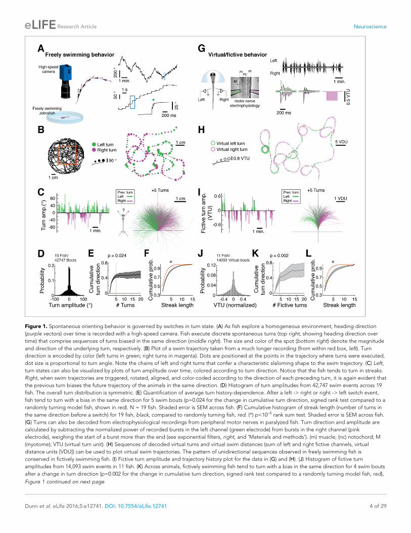
Figure 1. Spontaneous orienting behavior is governed by switches in turn state. (A) As fish explore a homogeneous environment, heading direction
(purple vectors) over time is recorded with a high-speed camera. Fish execute discrete spontaneous turns (top right, showing heading direction over
time) that comprise sequences of turns biased in the same direction (middle right). The size and color of the spot (bottom right) denote the magnitude
and direction of the underlying turn, respectively. (B) Plot of a swim trajectory taken from a much longer recording (from within red box, left). Turn
direction is encoded by color (left turns in green; right turns in magenta). Dots are positioned at the points in the trajectory where turns were executed;
dot size is proportional to turn angle. Note the chains of left and right turns that confer a characteristic slaloming shape to the swim trajectory. (C) Left,
turn states can also be visualized by plots of turn amplitude over time, colored according to turn direction. Notice that the fish tends to turn in streaks.
Right, when swim trajectories are triggered, rotated, aligned, and color-coded according to the direction of each preceding turn, it is again evident that
the previous turn biases the future trajectory of the animals in the same direction. (D) Histogram of turn amplitudes from 42,747 swim events across 19
fish. The overall turn distribution is symmetric. (E) Quantification of average turn history-dependence. After a left -> right or right -> left switch event,
fish tend to turn with a bias in the same direction for 5 swim bouts (p=0.024 for the change in cumulative turn direction, signed rank test compared to a
randomly turning model fish, shown in red). N = 19 fish. Shaded error is SEM across fish. (F) Cumulative histogram of streak length (number of turns in
the same direction before a switch) for 19 fish, black, compared to randomly turning fish, red. (*) p<10–5 rank sum test. Shaded error is SEM across fish.
(G) Turns can also be decoded from electrophysiological recordings from peripheral motor nerves in paralyzed fish. Turn direction and amplitude are
calculated by subtracting the normalized power of recorded bursts in the left channel (green electrode) from bursts in the right channel (pink
electrode), weighing the start of a burst more than the end (see exponential filters, right, and ’Materials and methods’). (m) muscle; (nc) notochord; M
(myotome); VTU (virtual turn unit). (H) Sequences of decoded virtual turns and virtual swim distances (sum of left and right fictive channels, virtual
distance units [VDU]) can be used to plot virtual swim trajectories. The pattern of unidirectional sequences observed in freely swimming fish is
conserved in fictively swimming fish. (I) Fictive turn amplitude and trajectory history plot for the data in (G) and (H). (J) Histogram of fictive turn
amplitudes from 14,093 swim events in 11 fish. (K) Across animals, fictively swimming fish tend to turn with a bias in the same direction for 4 swim bouts
after a change in turn direction (p=0.002 for the change in cumulative turn direction, signed rank test compared to a randomly turning model fish, red),
Figure 1 continued on next page
Dunn et al. eLife 2016;5:e12741. DOI: 10.7554/eLife.12741 4 of 29
Research Article Neuroscience
freely swimming conditions (modefictive/modefree = 1.4; meanfictive/meanfree = 2.4; medianfictive/
medianfree = 1.9), the large overlap between the histograms of inter-bout intervals (IBIs) (Figure 1—
figure supplement 4A–C) suggests that fictive behavior is sufficiently similar to that of freely swim-
ming fish to allow for analysis of concurrent neural signals.
Recording brain activity during spontaneous fictive locomotionWe used light-sheet microscopy to record neural activity in most neurons in the brain during sponta-
neous fictive locomotion. Using transgenic zebrafish expressing the genetically encoded calcium
indicator GCaMP6f or GCaMP6s (Chen et al., 2013) in most neurons (’Materials and methods’), and
a dual-laser light-sheet microscope capable of scanning the entire brain without exposing the retina
to the laser beam (Vladimirov et al., 2014) (Figure 2A), we captured whole-brain neuron-resolution
activity at 1.87 ± 0.14 (mean ± SD over all recordings) brain volumes per second during spontaneous
behavior (Video 2). To map the relationship between whole-brain activity and behavioral sequences,
we constructed a representation of swimming events that allows for nonlinear relationships between
neuronal activity and the strength and direction of turns. To generate this representation, fictive
recordings were transformed into distinct behavioral events (Ahrens et al., 2013) (Figure 2B, left;
’Materials and methods’), each associated with a particular point in a two-dimensional ’behavioral
tuning space’, analogous to a visual receptive field. In this space, angle represents turning direction,
and radial distance represents the strength of the motor event (Figure 2B, middle). By regressing
whole-brain activity against this representation
of behavior (Figure 2B, right; ’Materials and
methods’) (Portugues et al., 2014; Miri et al.,
2011), signals from individual voxels (or neurons)
were thus described with a tuning field over the
behavioral space (Figure 2C; two example neu-
rons, one tuned to left and the other to right
turns).
Whole-brain maps reveal neuralrepresentations of spontaneousbehaviorTo match neural activity to the pattern of spon-
taneous turning, we generated whole-brain
activity maps for individual fish by color-coding
each voxel for preferred angle (Figure 2D;
Videos 3,4; ’Materials and methods’; analysis
code and example data available online). We
encoded the predictability of the response, or
R2, with brightness so that brighter colors mean
Figure 1 continued
although many chains persist for much longer. N = 11 fish. Shaded error is SEM across fish. (L) The cumulative probability distribution of fictive streak
length is also significantly different from a randomly turning model fish. (*) p<10–4, rank sum test. N = 11 fish. Shaded error is SEM across fish.
DOI: 10.7554/eLife.12741.003
The following source data and figure supplements are available for figure 1:
Source data 1. Behavioral data from freely swimming larval zebrafish, with analysis code.
DOI: 10.7554/eLife.12741.004
Figure supplement 1. Analysis of free and fictive turn states.
DOI: 10.7554/eLife.12741.005
Figure supplement 2. Fictive swimming is a reliable readout of intended locomotion.
DOI: 10.7554/eLife.12741.006
Figure supplement 3. Fictive swims are not struggles or startles.
DOI: 10.7554/eLife.12741.007
Figure supplement 4. Comparison of free and fictive swimming statistics.
DOI: 10.7554/eLife.12741.008
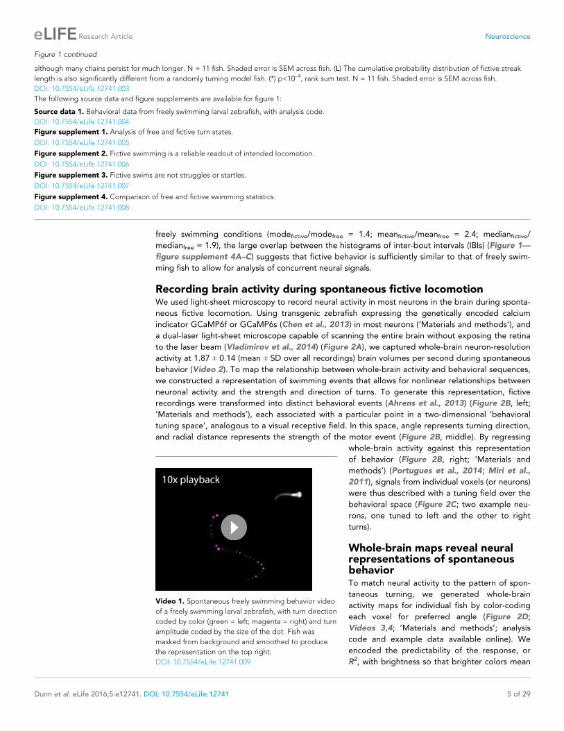
Video 1. Spontaneous freely swimming behavior video
of a freely swimming larval zebrafish, with turn direction
coded by color (green = left; magenta = right) and turn
amplitude coded by the size of the dot. Fish was
masked from background and smoothed to produce
the representation on the top right.
DOI: 10.7554/eLife.12741.009
Dunn et al. eLife 2016;5:e12741. DOI: 10.7554/eLife.12741 5 of 29
Research Article Neuroscience
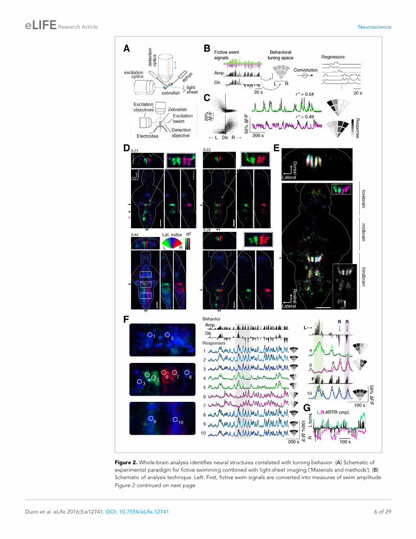
Figure 2. Whole-brain analysis identifies neural structures correlated with turning behavior. (A) Schematic of
experimental paradigm for fictive swimming combined with light-sheet imaging (’Materials and methods’). (B)
Schematic of analysis technique. Left: First, fictive swim signals are converted into measures of swim amplitude
Figure 2 continued on next page
Dunn et al. eLife 2016;5:e12741. DOI: 10.7554/eLife.12741 6 of 29
Research Article Neuroscience

more significant correlations to behavior (Figure 2D–F). These maps revealed the organization of
behavioral tuning in both neurons and neuropil. Neurons linked to spontaneous swimming were
located in diverse areas of the brain (Figure 2D–G). Anatomical consistency of the functionally iden-
tified regions was evaluated using a nonlinear volume registration algorithm (Portugues et al.,
2014) that aligned seven brains based only on anatomy; this analysis revealed that, across fish, the
most spatially conserved functionally defined cell clusters were in a region in the anterior hindbrain
(Figure 2E; Figure 2—figure supplement 2). This region is composed of two bilaterally symmetric
clusters of cells on either side of the midline. In a previous study (Ahrens et al., 2013), this area was
identified by brain activity alone – without behavioral readout – and termed the hindbrain oscillator
(HBO). The dynamics of these cells were tightly coupled to the direction of turning and highly anti-
phasic, such that the majority of the time, cells in only one hemisphere were active (Figure 2F,G).
The location and dynamics of these cells, which we call the anterior rhombencephalic turning region
(ARTR), named according to its salient anatomical and functional properties, was additionally verified
using two-photon imaging during fictive behavior (Figure 2—figure supplement 1). We manually
counted the numbers of neurons in the functional brain maps and found 60 ± 7 neurons in each
medial cluster and 33 ± 2 neurons in each lateral cluster (mean ± SEM, 8 fish). To visualize the
Figure 2 continued
(’Amp’) and turning direction (’Dir’ for laterality). Middle: Next, amplitude and laterality are mapped onto the
vertical and horizontal axes of a 2D space. This space is tiled with 12 basis functions, each representing a region in
this 2D behavior space, now defined in polar coordinates (’Materials and methods’). Contours are shown for
clarity; actual basis functions overlap by 50%. Right: The signal from each bin is convolved with an impulse
response function to generate a regressor; an example subset of regressors is shown. (C) Brain activity is regressed
against the regressors constructed in (B) to generate a behavioral tuning function for every voxel. Voxels of two
example neurons are shown here. Left, relationship between turn laterality and neural response for the two
example neurons, each dot is a time point. Middle, time series from the same two example neurons. Black line,
DF/F; colored line, prediction of best-fitting model (see panel B). Right, behavioral tuning for the same two
neurons, given by regression coefficients, using the analysis described in panel B; grayscale ranges from 10th to
90th percentile of the coefficient weights. (D) Behavioral tuning maps across the brain derived from fitting every
voxel with the regressors described in panel B, for four representative fish. Calcium indicators are either localized
in cytoplasm (left two fish) or in the nucleus (right two fish). The dorsal view is a maximum intensity projection over
the whole brain; the side and front views are taken from a maximum intensity projection of 21 slices ( ~ 10 mm)
along the medial-lateral axis and rostral-caudal axis, respectively. Numbers above each panel indicate the R2 value
at which the color map saturates (maximum R2 value is higher), color maps start at R2 = 0. Arrows in each panel
represent the centroid position of these slices for the frontal view (top) or side view (right). Solid arrowhead:
diffusive correlated region in rhombomeres 4–6. Open arrowhead, inferior olive. Scale bar, 100 mm. D, dorsal; V,
ventral; A, anterior; P, posterior. (E) Registered map from seven different fish (nuclear localized GCaMP6f) to a
standard brain. Each fish is encoded by a different color; brightness represents R2. Bottom, top-down maximum
intensity projection (along the dorsal-ventral axis). Top, front projection as in d, with the centroid of the slice
indicated by the arrow in bottom panel. Top right inset, ARTR region across fish in the standard brain, but with
color representing laterality as in panel d, showing consistent tuning across animals. Bottom right inset, a measure
of stereotypy in location of functionally identified neurons across the 7 fish. Intensity represents the standard
deviation divided by the mean of R2 (thresholded at 0.04). Scale bar, 100 mm. (F) Example DF/F traces from regions
of interest (ROIs) in panel (D) (left bottom, white boxes). Left, top to bottom: midbrain, ARTR, and caudal
hindbrain. Middle, top, signals of swim amplitude (Amp.) and turn laterality (Dir.). Black bars represent several
individual swim events. Bottom, DF/F from ROIs in the left panels. Right, enlarged view of gray region in middle
panel. L,R,F stand for left turns, right turns and swim amplitude, respectively. Responses from ROIs 1–3 and 8–10
show tuning to swim amplitude; ROIs 4,5 to left turns, and ROIs 6,7 to right turns. (G) In addition to single cells,
activity of left and right populations derived with ICA (Figure 2—figure supplement 1C–E; bottom-right fish of
Figure 2D) tracks turning behavior.
DOI: 10.7554/eLife.12741.010
The following figure supplements are available for figure 2:
Figure supplement 1. Alignment of functional brain maps in fish expressing calcium indicators in the cytosol.
DOI: 10.7554/eLife.12741.011
Figure supplement 2. Recovering the ARTR using supervised and unsupervised methods.
DOI: 10.7554/eLife.12741.012
Figure supplement 3. Dynamics of ARTR activity during behavior.
DOI: 10.7554/eLife.12741.013
Dunn et al. eLife 2016;5:e12741. DOI: 10.7554/eLife.12741 7 of 29
Research Article Neuroscience

relationship between ARTR dynamics at the time
of turns, we aligned the neuronal activity traces
to individual turns that were followed by five
seconds of no turns. At the time of a turn, the
ipsilateral ARTR was activated, and after a rise in
calcium signal over about 2 s, decayed to base-
line slowly on a timescale of 5–10 s (Figure 2—
figure supplement 3).
To analyze the wider anatomical features of
these maps across fish, we used Z-Brain (Fig-
ure 3—figure supplement 1) (Randlett et al.,
2015) to register together and average multiple
brain volumes. These averaged functional brain
maps (Figure 3A–B) revealed that the most
prominent directionally tuned neurons were
located in the hindbrain, where most tuning was
ipsilateral to turning direction. These prominent
directionally tuned neurons were found in the
ARTR in rhombomeres 2–3, diffusely distributed
in rhombomeres 4–6 (Rh4-6), in the inferior olive
(IO), and in the vicinity of and overlapping with
the reticulospinal system (Figure 3C,E). Weaker
and less directionally tuned signals were
observed in the torus longitudinalis, the habe-
nula, the preoptic area and pretectum, the cere-
bellum (Cb, Figure 3D), and the midbrain tegmentum, including the area containing the nucleus of
the medial longitudinal fasciculus (nMLF, Figure 3E, Figure 3—figure supplement 2).
These maps outline areas across the brain that are active during spontaneous locomotion, but
which of these areas may underlie the slow structure in directional swimming? The strongest direc-
tional tuning was found in the ARTR, Rh4-6, and IO. Directly comparing the directional tuning of the
ARTR and Rh4-6, however, revealed that the ARTR was more directionally tuned (Figure 3—figure
supplement 3A). In addition, the ARTR was more predictive of future turn direction (Figure 3—fig-
ure supplement 3B). These observations suggest that the ARTR may be more involved in turn pat-
terning. In addition, we compared the temporal dynamics of the ARTR and Rh4-6 and found that the
ARTR had slower dynamics than Rh4-6 (Figure 3—figure supplement 3C), suggesting that the
ARTR may be more involved in the slow dynamics of the behavior and Rh4-6 more in direct behav-
ioral output. Further, while the IO was strongly directionally tuned, it projects only to the contralat-
eral Cb (De Zeeuw et al., 1998; Bae et al., 2009). While we did see directional tuning with flipped
laterality in the Cb (Figure 3D), this signal was only weakly tuned to behavior, and therefore, the IO-
Cb circuit may be less directly related to turn
patterns. These results led to the hypothesis that
the ARTR might generate the slowly fluctuating
bias in swimming direction.
Video 2. Whole-brain imaging during spontaneous
fictive behavior recorded in the light-sheet virtual
reality setup. Left: top projection of whole-brain DF/F.
Top left: behavior represented by left and right turn
amplitude. Right: projections of whole-brain DF/F,
where the brain has been masked by the R2 volume, so
that each voxel represents DF/F x R2, emphasizing
neural activity in the regions identified by the
regression analysis.
DOI: 10.7554/eLife.12741.014
Video 3. Analysis of imaging data Computational brain
maps of the voxel-wise tuning to the laterality of turns.
Green signifies tuning to left turns; magenta to right
turns; brightness codes for R2 of the model fit. Same
data as Figure 2 but represented in three dimensions.
DOI: 10.7554/eLife.12741.015
Video 4. 3D representation of Z-Brain atlas.
DOI: 10.7554/eLife.12741.016
Dunn et al. eLife 2016;5:e12741. DOI: 10.7554/eLife.12741 8 of 29
Research Article Neuroscience
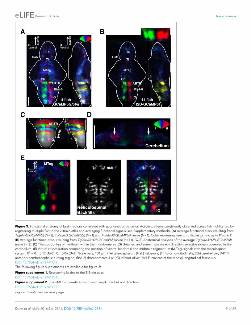
Figure 3. Functional anatomy of brain regions correlated with spontaneous behavior. Activity patterns consistently observed across fish highlighted by
registering multiple fish to the Z-Brain atlas and averaging functional signals (see Supplementary methods). (A) Average functional stack resulting from
Tg(elavl3:GCaMP6f) (N=2), Tg(elavl3:GCaMP5G) (N=1) and Tg(elavl3:GCaMP6s) larvae (N=1). Color represents tuning to fictive turning as in Figure 2.
(B) Average functional stack resulting from Tg(elavl3:H2B-GCaMP6f) larvae (n=11). (C–E) Anatomical analyses of the average Tg(elavl3:H2B-GCaMP6f)
maps in (B). (C) The positioning of hindbrain within the rhombomeres. (D) Untuned and some more weakly direction selective signals observed in the
cerebellum. (E) Virtual colocalization comparing the position of ventral hindbrain and midbrain tegmentum (M-Teg) signals with the reticulospinal
system. R2 = 0. . .0.12 (A–C), 0. . .0.06 (D–E). Scale bars, 100 mm. (Te) telencephalon; (Hab) habenula; (Tl) torus longitudinalis; (Cb) cerebellum; (ARTR)
anterior rhombencephalic turning region; (Rh4-6) rhombomeres 4-6; (IO) inferior olive; (nMLF) nucleus of the medial longitudinal fasciculus.
DOI: 10.7554/eLife.12741.017
The following figure supplements are available for figure 3:
Figure supplement 1. Registering brains to the Z-Brain atlas.
DOI: 10.7554/eLife.12741.018
Figure supplement 2. The nMLF is correlated with swim amplitude but not direction.
DOI: 10.7554/eLife.12741.019
Figure 3 continued on next page
Dunn et al. eLife 2016;5:e12741. DOI: 10.7554/eLife.12741 9 of 29
Research Article Neuroscience
The ARTR biases spontaneous turningThe relationship between neuronal activity in the ARTR and fictive behavior suggests that the ARTR
may underlie directionality in spontaneous swimming, such that activity in the right ARTR or the left
ARTR biases turning to the right or the left, respectively. To test this hypothesis, we performed uni-
lateral lesions of the ARTR. To do this, we first functionally identified the ARTR at the single-cell level
in each fish, using two-photon imaging and fast analyses of correlated activity patterns (’Materials
and methods’). This enabled us to use targeted two-photon laser ablation to lesion one side of the
ARTR while keeping the other side intact (19 ± 6 cells [mean ± SD] in the medial cluster, i.e. about
32% of cells of one medial cluster; ’Materials and methods’). Freely swimming behavior was quanti-
fied before and after unilateral lesions of the ARTR. We found that post-ablation, fish turned rela-
tively more often toward the direction of the intact half of the ARTR (shift in turn direction to intact
side: 18 ± 4%, mean ± SEM; Figure 4A–B) (left ARTR ablation: N = 6 fish, p=0.031; right ARTR abla-
tion: N = 7 fish, p=0.031; sham ablation: N = 5, p=0.438, paired signed rank test), suggesting that
the ARTR is involved in generating directionality bias in spontaneous turning behavior.
Do these ARTR lesions affect the turn bias, or simply the ability of the animals to turn? We exam-
ined the magnitude of turns – independent of relative frequency – pre- and post-ablation. In contrast
to the effect of reticulospinal neuron ablation (Orger et al., 2008; Huang et al., 2013;
Kimmel et al., 1982), after ARTR ablation, the magnitude of turns to either the ablated or intact
side remained unchanged (Figure 4C, p=0.147, ablated side; p=0.127, intact side, N = 13 fish,
paired signed rank test). These results suggest that the ARTR is involved in regulating the choice of
turning direction, rather than mediating the actual turn kinematics.
We also tested whether the ARTR contributes to temporal correlations in turn direction. For each
fish, before and after ablation, we constructed a model fish consisting of a history-independent pro-
cess in which every turn was randomly chosen to be to the left or to the right. Since the overall turn
bias contributes to the distribution of streak lengths, the bias of each model fish must be matched
to that of each real fish. Thus, the direction of every turn in each model fish effectively results from a
biased coin flip, with the bias matched to each corresponding real fish (e.g. 45% right turns and 55%
left turns). Under the hypothesis that the ARTR contributes to temporal correlations in turn direction,
the streak length distribution of a post-ablation real fish should be closer to that of its matched
model fish than a pre-ablation real fish to its matched model fish. We found that this was indeed the
case (Figure 4D–F). Specifically, comparing the goodness-of-fit between the matched biased ran-
dom walks and the observed turn sequences (’Materials and methods’), we found a significant reduc-
tion in the normalized root-mean-square error over fish after ablation (Figure 4G, p=0.027, paired
signed rank test, N = 13 fish). These results indicate that turn sequences in lesioned fish are more
similar to strings of biased coin flips than are turn sequences in intact fish, providing evidence that
the ARTR is part of a circuit that implements a temporally correlated process.
To further test whether the ARTR biases turn direction, we optogenetically stimulated the ARTR
in fish expressing both GCaMP6f and the excitatory opsin ReaChR (Lin et al., 2013) under the elavl3
promoter (’Materials and methods’). We first imaged the area of the ARTR using 930 nm light (near
the peak two-photon excitation wavelength of GCaMP6f) and functionally identified ARTR neurons.
Next, we selected an ROI over 15 to 20 ARTR neurons and stimulated these neurons using 1050 nm
light (near the peak two-photon excitation wavelength of ReaChR). Stimulating ARTR cells caused an
increase in the number of turns in the direction ipsilateral to the stimulated ARTR region
(Figure 4H–K; 29 ± 9%, mean ± SEM, shift in turns to the stimulated direction; left stimulation,
p=0.004; right stimulation, p=0.002, paired signed rank test, N = 7 fish), independent of whether
the medial clusters or lateral clusters were chosen for stimulation (Figure 4—figure supplement
1A). These results are corroborated by electrical stimulation experiments (Figure 4—figure supple-
ment 1B–D), demonstrating that the ARTR is functionally connected to downstream motor circuitry
and that activity in the ARTR influences turn direction. In contrast to our ablation results, the magni-
tude of turns during stimulation of the medial clusters tended to increase (Figure 4L, Figure 4—fig-
ure supplement 1A, left stimulation, p=0.010; right stimulation, p=0.036, paired signed rank test, N
Figure 3 continued
Figure supplement 3. Comparison of ARTR and Rh4-6 dynamics, tuning, and predictiveness of future behavior.
DOI: 10.7554/eLife.12741.020
Dunn et al. eLife 2016;5:e12741. DOI: 10.7554/eLife.12741 10 of 29
Research Article Neuroscience
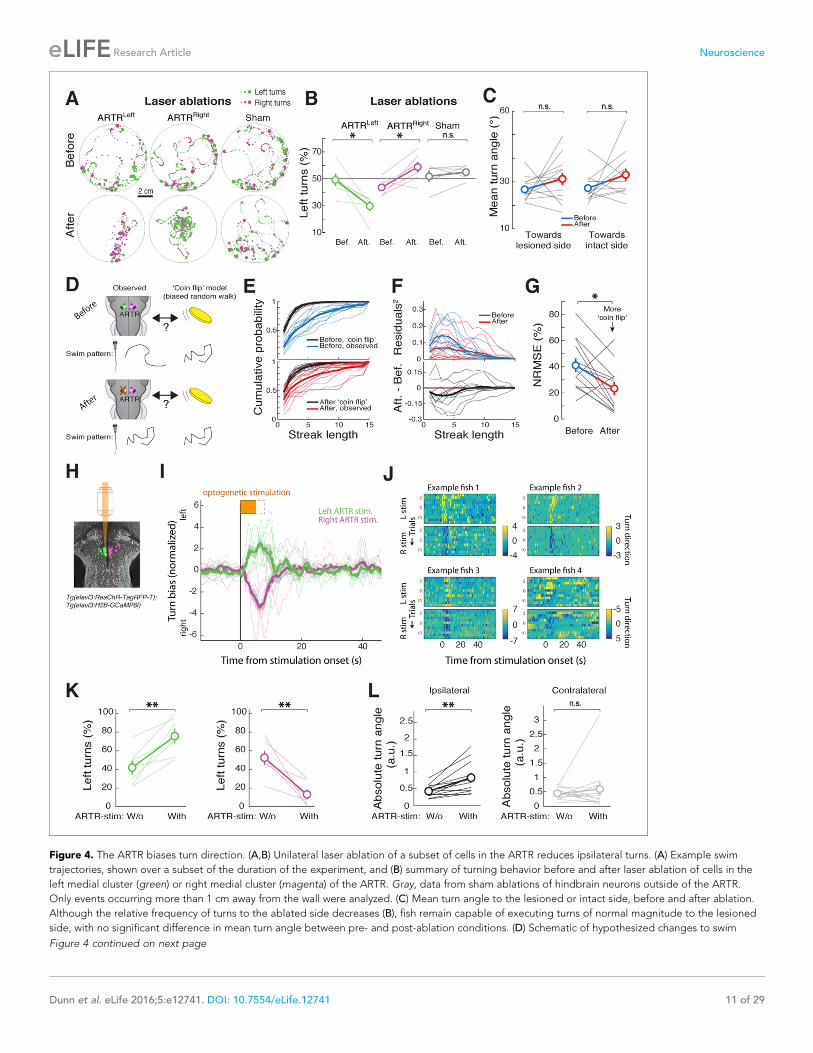
Figure 4. The ARTR biases turn direction. (A,B) Unilateral laser ablation of a subset of cells in the ARTR reduces ipsilateral turns. (A) Example swim
trajectories, shown over a subset of the duration of the experiment, and (B) summary of turning behavior before and after laser ablation of cells in the
left medial cluster (green) or right medial cluster (magenta) of the ARTR. Gray, data from sham ablations of hindbrain neurons outside of the ARTR.
Only events occurring more than 1 cm away from the wall were analyzed. (C) Mean turn angle to the lesioned or intact side, before and after ablation.
Although the relative frequency of turns to the ablated side decreases (B), fish remain capable of executing turns of normal magnitude to the lesioned
side, with no significant difference in mean turn angle between pre- and post-ablation conditions. (D) Schematic of hypothesized changes to swim
Figure 4 continued on next page
Dunn et al. eLife 2016;5:e12741. DOI: 10.7554/eLife.12741 11 of 29
Research Article Neuroscience
= 7 fish), indicating that either the ARTR is able to bias turn magnitude in addition to turn direction,
or that there is a spillover of artificial ARTR stimulation to downstream circuits.
ARTR neurotransmitter identity and morphologyGiven these functional observations of ARTR activity and its effect on behavior, how might ARTR
connectivity give rise to its activity patterns and cause it to influence motor output? To address this
question, we investigated the projection patterns of ARTR cells to look for evidence of putative
intrinsic connectivity and putative connectivity to premotor neurons.
Registration to the Z-Brain atlas suggested a unique distribution of neurotransmitter identities
within the ARTR, which comprises a pair of medial and lateral clusters in both hemispheres. In the Z-
Brain atlas, the medial and lateral clusters mostly overlapped with glutamate and GABA markers,
respectively (Figure 5—figure supplement 1A,B). To verify this overlap, we functionally identified
the ARTR in double transgenic lines with GCaMP6f and red fluorescent labels for either glutamater-
gic (vglut2a) or GABAergic (gad1b) neurons and matched it with its neurotransmitter phenotype
(Figure 5A, Figure 5—figure supplement 1C,D, ’Materials and methods’). In this way, the medial
clusters of the ARTR were identified as being glutamatergic, and the lateral clusters as being primar-
ily GABAergic (Figure 5A middle and right, respectively).
How might such an arrangement of excitatory and inhibitory neurons lead to the activity patterns
observed in the ARTR? The strongly antiphasic activity patterns and the presence of excitatory and
inhibitory clusters suggests underlying mutual inhibition, i.e. when one side of the ARTR is active,
the other side is suppressed. To probe for such an architecture, we used a combination of calcium
imaging and photoactivateable GFP (PA-GFP) (Patterson, 2002; Ruta et al., 2010; Datta et al.,
2008). After functionally identifying the ARTR using a nuclear-localized calcium indicator (H2B-
GCaMP6f), we photoactivated PA-GFP in a subset of ARTR cells and traced their projections.
Indeed, tracing PA-GFP-activated neurites from the lateral GABAergic clusters revealed projections
reaching across the midline toward both contralateral ARTR clusters (Figure 5B and Figure 5—fig-
ure supplement 1E–G). In contrast, we did not find evidence for neurites from the medial glutama-
tergic clusters crossing the midline (Figure 5B, bottom right). Although these tracing studies cannot
prove whether there exists synaptic connectivity between the ARTR clusters, they are suggestive of
a mutually inhibitory circuit motif, which could mediate the antiphasic activation necessary for pat-
terning directional motor output.
To investigate potential connectivity between the ARTR and downstream premotor circuitry, we
again combined functional imaging with anatomical tracing, this time using PA-GFP with a red fluores-
cent calcium indicator (jRCaMP1a [Dana et al., 2016]), which improved our ability to trace more distal
Figure 4 continued
structure, assuming that the ARTR is involved in setting correlational patterns. Before and after ablation, turn patterns will be compared to a ‘coin flip’
model that emits turns to the left and right randomly but with some bias equal to the observed data. (E) Empirical cumulative distribution functions
(CDFs) of streak length before (blue, top) and after (red, bottom) ablation, compared to model fish executing turns at random without history
dependence but with overall turn bias matched to each individual fish (black). Streak length post-ablation appears distributed more like ’coin flips’. (F)
Top, quantification of the squared residuals between each individual fish CDF and its matched ’coin flip’ CDF before (blue) and after (red) ablation.
Bottom, the difference between each respective before and after curve reveals a shift toward the ’coin flip’ distribution for the majority of fish. (G)
Summary of the normalized root-mean-square error (NRMSE) quantifying goodness-of-fit between the observed streak distributions and their matched
random model distributions. After ablation, turning becomes more ‘coin flip’-like and thus history dependence is reduced. (H–L) Optogenetic
stimulation of the ARTR elicits ipsilateral turn biases. (H) The ARTR was functionally identified in double transgenic fish Tg(elavl3:H2B-GCaMP6f;elavl3:
ReaChR-TagRFP-T) and a medial ARTR cluster was unilaterally stimulated. Gray, expression of ReaChR-TagRFP-T; green and magenta, functionally
identified ARTR from this example fish based on correlational map. (I) Ipsilateral turn bias increases during optogenetic stimulation (solid lines, 5 s
stimulation; dotted lines, 8 s stimulation, N = 7 fish, ’Materials and methods’). (J) Results from example fish show the reproducibility of stimulation effect
across trials. Turn direction is normalized to time-averaged turn direction pre-stimulation. (K) Summary of the change in bias quantified for each fish,
showing that optogenetic stimulation results in a bias toward ipsilateral turns. (L) Summary of the change in absolute fictive turn angle during
stimulation, showing that ipsilateral turn angle increases and contralateral turn angle remains unchanged. n.s., no significance; (*) p<0.05; (**) p<0.01
(paired signed rank test). All error bars are mean ± SEM across fish.
DOI: 10.7554/eLife.12741.021
The following figure supplement is available for figure 4:
Figure supplement 1. Detailed analysis of ARTR stimulations.
DOI: 10.7554/eLife.12741.022
Dunn et al. eLife 2016;5:e12741. DOI: 10.7554/eLife.12741 12 of 29
Research Article Neuroscience
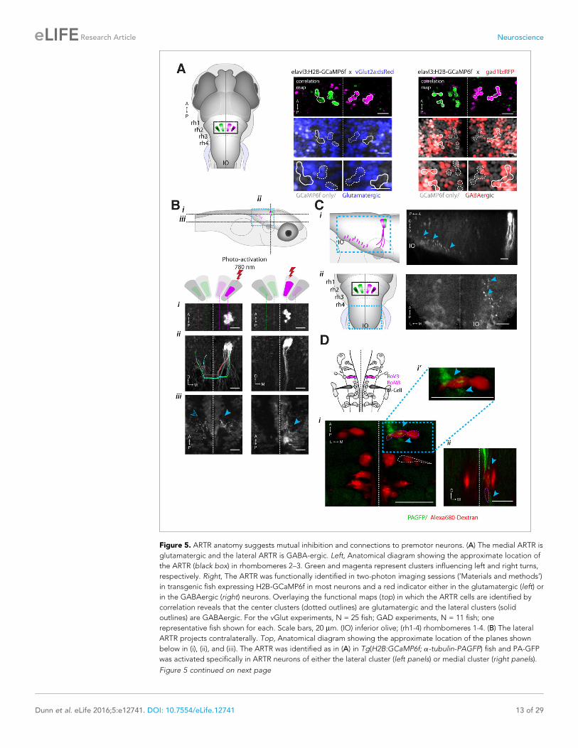
Figure 5. ARTR anatomy suggests mutual inhibition and connections to premotor neurons. (A) The medial ARTR is
glutamatergic and the lateral ARTR is GABA-ergic. Left, Anatomical diagram showing the approximate location of
the ARTR (black box) in rhombomeres 2–3. Green and magenta represent clusters influencing left and right turns,
respectively. Right, The ARTR was functionally identified in two-photon imaging sessions (’Materials and methods’)
in transgenic fish expressing H2B-GCaMP6f in most neurons and a red indicator either in the glutamatergic (left) or
in the GABAergic (right) neurons. Overlaying the functional maps (top) in which the ARTR cells are identified by
correlation reveals that the center clusters (dotted outlines) are glutamatergic and the lateral clusters (solid
outlines) are GABAergic. For the vGlut experiments, N = 25 fish; GAD experiments, N = 11 fish; one
representative fish shown for each. Scale bars, 20 mm. (IO) inferior olive; (rh1-4) rhombomeres 1-4. (B) The lateral
ARTR projects contralaterally. Top, Anatomical diagram showing the approximate location of the planes shown
below in (i), (ii), and (iii). The ARTR was identified as in (A) in Tg(H2B:GCaMP6f; a-tubulin-PAGFP) fish and PA-GFP
was activated specifically in ARTR neurons of either the lateral cluster (left panels) or medial cluster (right panels).
Figure 5 continued on next page
Dunn et al. eLife 2016;5:e12741. DOI: 10.7554/eLife.12741 13 of 29
Research Article Neuroscience
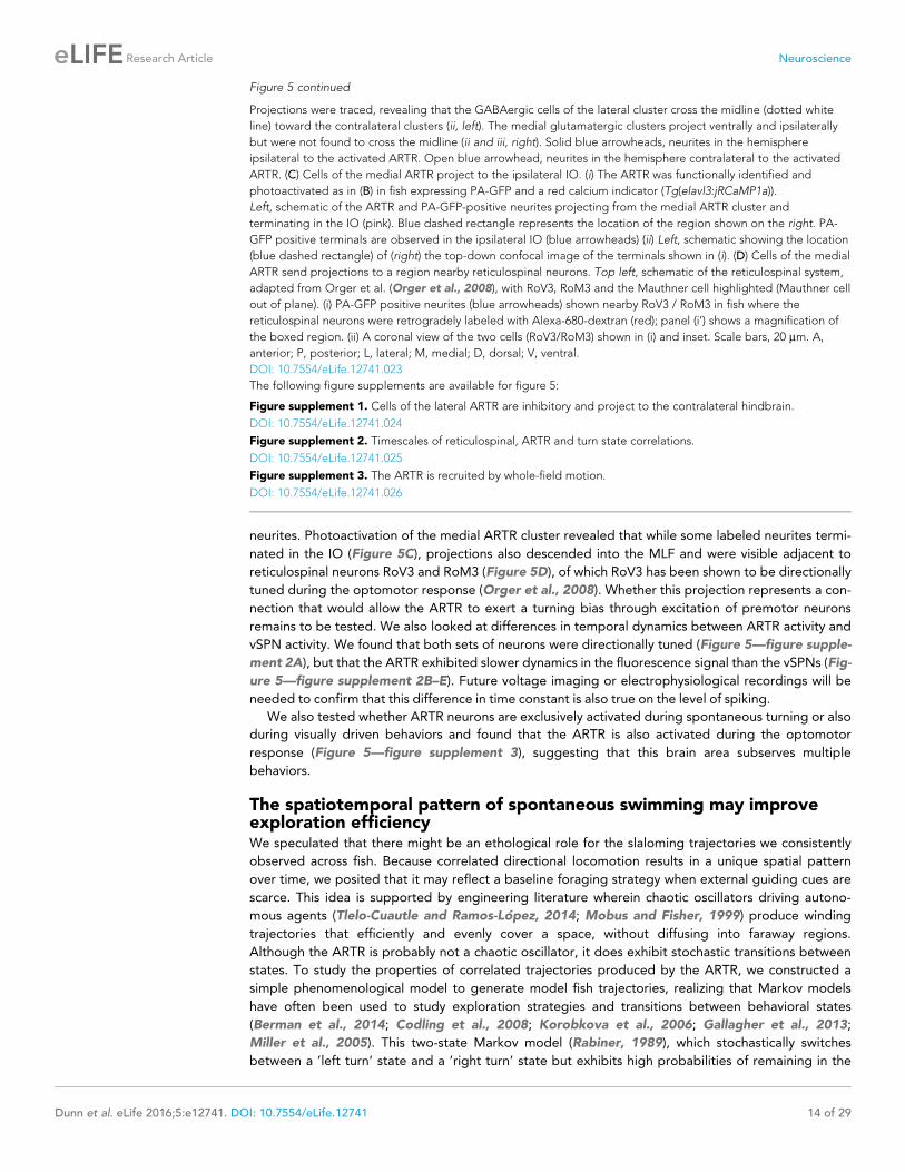
neurites. Photoactivation of the medial ARTR cluster revealed that while some labeled neurites termi-
nated in the IO (Figure 5C), projections also descended into the MLF and were visible adjacent to
reticulospinal neurons RoV3 and RoM3 (Figure 5D), of which RoV3 has been shown to be directionally
tuned during the optomotor response (Orger et al., 2008). Whether this projection represents a con-
nection that would allow the ARTR to exert a turning bias through excitation of premotor neurons
remains to be tested. We also looked at differences in temporal dynamics between ARTR activity and
vSPN activity. We found that both sets of neurons were directionally tuned (Figure 5—figure supple-
ment 2A), but that the ARTR exhibited slower dynamics in the fluorescence signal than the vSPNs (Fig-
ure 5—figure supplement 2B–E). Future voltage imaging or electrophysiological recordings will be
needed to confirm that this difference in time constant is also true on the level of spiking.
We also tested whether ARTR neurons are exclusively activated during spontaneous turning or also
during visually driven behaviors and found that the ARTR is also activated during the optomotor
response (Figure 5—figure supplement 3), suggesting that this brain area subserves multiple
behaviors.
The spatiotemporal pattern of spontaneous swimming may improveexploration efficiencyWe speculated that there might be an ethological role for the slaloming trajectories we consistently
observed across fish. Because correlated directional locomotion results in a unique spatial pattern
over time, we posited that it may reflect a baseline foraging strategy when external guiding cues are
scarce. This idea is supported by engineering literature wherein chaotic oscillators driving autono-
mous agents (Tlelo-Cuautle and Ramos-Lopez, 2014; Mobus and Fisher, 1999) produce winding
trajectories that efficiently and evenly cover a space, without diffusing into faraway regions.
Although the ARTR is probably not a chaotic oscillator, it does exhibit stochastic transitions between
states. To study the properties of correlated trajectories produced by the ARTR, we constructed a
simple phenomenological model to generate model fish trajectories, realizing that Markov models
have often been used to study exploration strategies and transitions between behavioral states
(Berman et al., 2014; Codling et al., 2008; Korobkova et al., 2006; Gallagher et al., 2013;
Miller et al., 2005). This two-state Markov model (Rabiner, 1989), which stochastically switches
between a ’left turn’ state and a ’right turn’ state but exhibits high probabilities of remaining in the
Figure 5 continued
Projections were traced, revealing that the GABAergic cells of the lateral cluster cross the midline (dotted white
line) toward the contralateral clusters (ii, left). The medial glutamatergic clusters project ventrally and ipsilaterally
but were not found to cross the midline (ii and iii, right). Solid blue arrowheads, neurites in the hemisphere
ipsilateral to the activated ARTR. Open blue arrowhead, neurites in the hemisphere contralateral to the activated
ARTR. (C) Cells of the medial ARTR project to the ipsilateral IO. (i) The ARTR was functionally identified and
photoactivated as in (B) in fish expressing PA-GFP and a red calcium indicator (Tg(elavl3:jRCaMP1a)).
Left, schematic of the ARTR and PA-GFP-positive neurites projecting from the medial ARTR cluster and
terminating in the IO (pink). Blue dashed rectangle represents the location of the region shown on the right. PA-
GFP positive terminals are observed in the ipsilateral IO (blue arrowheads) (ii) Left, schematic showing the location
(blue dashed rectangle) of (right) the top-down confocal image of the terminals shown in (i). (D) Cells of the medial
ARTR send projections to a region nearby reticulospinal neurons. Top left, schematic of the reticulospinal system,
adapted from Orger et al. (Orger et al., 2008), with RoV3, RoM3 and the Mauthner cell highlighted (Mauthner cell
out of plane). (i) PA-GFP positive neurites (blue arrowheads) shown nearby RoV3 / RoM3 in fish where the
reticulospinal neurons were retrogradely labeled with Alexa-680-dextran (red); panel (i’) shows a magnification of
the boxed region. (ii) A coronal view of the two cells (RoV3/RoM3) shown in (i) and inset. Scale bars, 20 mm. A,
anterior; P, posterior; L, lateral; M, medial; D, dorsal; V, ventral.
DOI: 10.7554/eLife.12741.023
The following figure supplements are available for figure 5:
Figure supplement 1. Cells of the lateral ARTR are inhibitory and project to the contralateral hindbrain.
DOI: 10.7554/eLife.12741.024
Figure supplement 2. Timescales of reticulospinal, ARTR and turn state correlations.
DOI: 10.7554/eLife.12741.025
Figure supplement 3. The ARTR is recruited by whole-field motion.
DOI: 10.7554/eLife.12741.026
Dunn et al. eLife 2016;5:e12741. DOI: 10.7554/eLife.12741 14 of 29
Research Article Neuroscience

Figure 6. Correlated turn states may underlie efficient local exploration (A) Spontaneous turn states are well-characterized by a two-state Markov
model (Figure 6—figure supplement 1). In an average model fit, fish in the left state, SL, are much more likely ( ~ 90%) to turn left (eL) than right (eR),
and vice-versa. And fish in SL or SR tend to return to SL or SR, respectively, after a turn. (B) Left, black, Five swim trajectories generated with a Markov
model matching the statistics of acquired swim data (see fish 16, Figure 6—figure supplement 1, Ptransition = [PL"L PL"R PR"L PR"R] = [0.86 0.14 0.15
0.85]). Right, blue, five swim trajectories generated with a Markov model randomly emitting left and right turns (all Ptransition = 0.5). Notice that the
unadjusted ’random’ fish diffuses farther from the given starting position. The dotted circle represents the mean diffusion distance for the correlated
model fish. All trajectories begin at the center of the circle and facing in the direction of the arrow. (C) Left, five example trajectories from the ’random’
model fish after average diffusion has (right) been matched to the correlated fish by decreasing bout distance. (D) Plots of exploration efficiency for
the ’random’ model fish normalized by bout distance. Left, in this local regime, the ’random’ model fish must turn more (16.9% more for 1 resource,
p < 10–9; p = 0.004 for 10 resources, two-tailed t-test) and (right) execute more swim bouts (21.3% fewer resources after 40 swims, p=<10–9, two-tailed t-
test) than the correlated model to collect randomly distributed virtual resources. Left, dashed lines, plots showing the proportion of simulated
trajectories able to gather the indicated number of resources after 40 swims. Error bars are SEM, see Figure 6—figure supplement 1E,F; ’Materials
and methods’. (E) Left, five example trajectories from the ’random’ model fish after average diffusion has (right) been matched to the correlated model
fish by broadening the underlying turn angle distribution. (F) Plots of exploration efficiency for the ’random’ model fish normalized by turn angle. Left,
this ’random’ fish must turn much more (40.8% more for 1 resource, p<10–9; p<10–9 for 10 resources, two-tailed t-test) and (right) execute more swim
bouts (7.0% fewer resources after 40 swims, p=9.9 � 10–4, two-tailed t-test) than the correlated model to collect randomly distributed virtual resources.
Left, dashed lines, plots showing the proportion of simulated trajectories able to gather the indicated number of resources after 40 swims. Error bars
are SEM, see Figure 6—figure supplement 1G,H; ’Materials and methods’.
DOI: 10.7554/eLife.12741.027
The following figure supplement is available for figure 6:
Figure supplement 1. Validation of two-state Markov model.
DOI: 10.7554/eLife.12741.028
Dunn et al. eLife 2016;5:e12741. DOI: 10.7554/eLife.12741 15 of 29
Research Article Neuroscience

same turn state (Figure 6A; Figure 6—figure supplement 1A, ’Materials and methods’), produced
behavior similar to that of real fish (Figure 6—figure supplement 1B,C) based only on low-level
parameters. Using this Markov model to simulate trajectories through virtual space (Figure 6B), we
show that such a scheme covers a restricted area more efficiently than a model fish turning left and
right randomly without turn history dependence, and reduces diffusion into faraway regions
(Figure 6C–F, Figure 6—figure supplement 1E–H). This strategy presents two distinct advantages.
First, rapid spatial diffusion may lead the fish into unknown and potentially unsafe territories; this
should be prevented. Second, given this preference to remain local, covering an area efficiently in
the search for food cues represents an energetically favorable program that ensures no nearby
resources have been missed. Thus, we speculate that the ARTR is part of a circuit that implements a
foraging strategy that discourages travel into uncertain territory, instead favoring efficient and even
exploration of the local environment.
DiscussionWe uncovered an anatomically and functionally defined population of neurons that we propose is part
of a circuit generating the spontaneous, patterned statistics of a directional locomotion behavior. We
speculate that the function of the ARTR is to coordinate multiple successive swim bouts in order to
shape trajectories on spatial scales larger than individual locomotor events. Analogous behavioral
strategies must exist in other animals that explore environments much larger than themselves
(Flavell et al., 2013; Stephens, 1986; Charnov, 1976). Thus, we expect that neural systems coordi-
nating the transformation of multiple local actions into global actions also exist in other organisms.
The challenge in identifying neural circuits underlying such behavior lies both in the characteriza-
tion of the behavior (Stephens et al., 2008) and in locating neural structures implementing observed
behavioral schema. Spontaneously active single neurons in primates (Okano and Tanji, 1987) and
invertebrates (Kagaya and Takahata, 2011) have been studied in concert with behavior, as well as
neurons in invertebrates that trigger behaviors such as escape responses, exploratory limb move-
ments and particular walking patterns (Berg et al., 2015; Bidaye et al., 2014; Fotowat and Gab-
biani, 2011). Here, we harnessed the power of fast whole-brain imaging to describe, in detail, a
nucleus in the zebrafish hindbrain influencing a simple but potentially vital behavioral algorithm that
may optimize foraging when available information about the environment is scarce.
We hypothesize that the ARTR contributes to the control of correlations in turn direction accord-
ing to the following mechanism. Activity on one side of the ARTR biases turn direction by subthresh-
old excitation of reticulospinal neurons by the medial cluster of cells. When the fish turns in the
direction where the ARTR is active, a motor copy feeds back on the ipsilateral ARTR and re-activates
it, which also suppresses the contralateral ARTR through contralateral inhibition. Next, ARTR activity
decays slowly, again biasing turns to the same direction. This scheme could generate sequences of
turns in the same direction. Switches in turn direction might arise from spontaneous activity in
the ARTR population, from spontaneous or evoked input from neurons upstream of the ARTR, or
when ARTR activity has decayed sufficiently so that it no longer exerts a bias on turning direction. To
test this model, synaptic connections between ARTR clusters and between the ARTR and vSPNs
need to be established, and ARTR activation and decay dynamics must be carefully characterized
using electrophysiology. It should also be determined, for example with the aid of optogenetic
silencing, whether the ARTR operates autonomously or whether it relies on interactions with other
populations, such as cells in Rh4-6.
Comprehensive, whole-brain, cell-level imaging was crucial for discovering the ARTR circuit
(Vladimirov et al., 2014; Freeman et al., 2014). Lacking a priori hypotheses regarding the location of
circuits governing a behavior, the near-complete coverage of this approach helps ensure that neurons
with response properties of interest, if present, will likely be identified (depending on the sensitivity of
the activity reporter [Chen et al., 2013] and the design of computational approaches [Freeman et al.,
2014]). Thus, while inputs to the identified neural populations certainly shape circuit activity, our meas-
urements and analyses suggest that the identified cells are likely to be the primary set of neurons con-
sistently involved in generating directional behavior. Of these neurons, we decided to causally
interrogate the ARTR because of its strong stereotypy across fish, tight correlations to the slow switch-
ing structure of spontaneous behavior, and its pattern of projections to the premotor reticulospinal
system. We identified, by ablation and stimulation, the ability of the ARTR to bias turning direction.
Dunn et al. eLife 2016;5:e12741. DOI: 10.7554/eLife.12741 16 of 29
Research Article Neuroscience
The properties of the ARTR, including its morphological projections, activation after a turn, ability to
bias turns, and slow decay time, together with the change in the temporal structure of behavior follow-
ing ARTR lesions, establishes the ARTR as an important candidate for the circuit generating temporal
structure in spontaneous turn sequences. However, the ARTR may also be part of a larger circuit per-
forming this operation. The contribution of other functionally identified regions, which were mapped
carefully across fish utilizing the Z-brain atlas, will be explored in future studies.
Tethered preparations are an important tool for studying the relationship between neuronal activ-
ity and behavior (Dombeck and Reiser, 2012). Differences between real and tethered behaviors are
usually present (Dombeck and Reiser, 2012), but are, in many cases, small enough to allow for the
study of related neural activity, including for relatively complex phenomena such as spatial represen-
tations (Seelig and Jayaraman, 2015; Harvey et al., 2009). Here, we observed differences between
the fictive behavior and freely swimming behavior, such as an approximately 1.4- to 2.4-fold differ-
ence in swim frequency, but these differences were modest enough for the essential properties of
the behavior to persist, allowing the underlying signals to be analyzed. Since the length of behavioral
sequences was similar when analyzed over number of swim bouts, it is possible that the time con-
stant of the ARTR was slightly longer in the fictively behaving fish, potentially due to influences such
as a lack of proprioceptive feedback. However, the persistent similarity of behavioral sequences and
other behavioral kinematics (Figure 1—figure supplement 4D,E) between fictively and freely swim-
ming fish suggests that the function of neural circuits underlying behavior remain largely intact under
the microscope. Of course, subsequent perturbation studies, like the ones performed here, are cru-
cial for establishing the necessity or sufficiency of neurons for a given behavior.
Based on PA-GFP tracing, neurotransmitter phenotyping, and references to the Z-Brain atlas, we
have developed predictions for specific connectivity between the medial and lateral ARTR clusters,
and the medial ARTR cluster and downstream reticulospinal premotor neurons. Deciphering the
nature of these connections will be essential for a precise mechanistic understanding of ARTR
dynamics and their link to spontaneous behavioral bias. Future experiments employing electrophysi-
ology, viral tracing, and connectomics will verify and expand on the precise mechanistic operations
of the circuits underlying spontaneous behavior in larval zebrafish.
The initiation of locomotion in other animals, such as lamprey (Sirota et al., 2000), salamander
(Cabelguen et al., 2003), and cat (Shik et al., 1969), has been attributed to the mesencephalic loco-
motor region (MLR). While the MLR has yet to be identified in the larval zebrafish (Severi et al.,
2014), the midbrain tegmental nMLF has been shown to regulate swimming (Severi et al.,
2014; Thiele et al., 2014; Wang and McLean, 2014). Consistent with this, we find the nMLF to be
routinely correlated with spontaneous swimming, and it is possible that the additional mesencephalic
cells not part of the nMLF but correlated strongly with swim amplitude (Figure 3E, Figure 3—figure
supplement 2) may be part of the larval zebrafish MLR. Furthermore, motor-related signals were
present, albeit weakly, in other areas including in the forebrain; it will be exciting to discover
whether these areas, or even the ARTR itself, are homologous to structures known to be involved in
motor control in other species but have not yet been located in the larval zebrafish. That being said,
while we have reported a causal role of the ARTR in spontaneous swim patterns, we do not claim
that the initial command for motion originates from the ARTR. Rather, we suggest that the ARTR
exerts a bias on the direction of swim bouts initiated by other circuits. This view is supported data
presented in Figure 4—figure supplement 1A, bottom, which shows that additional turns are not
recruited by ARTR stimulation. Thus, we argue that the ARTR occupies a position complementary to
canonical motor control centers.
The neural populations uncovered by our analysis are involved in setting the direction of sponta-
neous swimming but may be involved in other functions as well. In principle, signals from other
motor modalities as well as sensory systems could be integrated into ARTR activity fluctuations. In
feature-poor environments, the ARTR system may interact with sensory systems in such a way that
ARTR control of exploration is preserved but biased by the influence of weak sensory inputs. When
stronger sensory cues are encountered, navigation systems purely driven by sensory stimulation may
take over. For instance, all or part of the cell population may be involved in the optomotor response,
as the ARTR responds to whole-field motion, and turns in the direction of motion persist after visual
stimuli disappear (Figure 5—figure supplement 3). In the context of phototaxis, navigational strate-
gies have been observed in larval zebrafish that also exhibit strong temporal correlations in turning
direction (Chen and Engert, 2014), potentially involving the ARTR. Furthermore, preliminary
Dunn et al. eLife 2016;5:e12741. DOI: 10.7554/eLife.12741 17 of 29
Research Article Neuroscience
observations show that eye movements (Miri et al., 2011) and turning are correlated in larval zebra-
fish, and activity in the vicinity of the abducens and oculomotor nuclei is correlated to turning and
ARTR activity (albeit much more weakly than the strength of correlation between the ARTR and turn-
ing, Figures 2,3). Thus, it is possible that multiple motor patterns are represented in and coordi-
nated by the ARTR. In the future, it will be exciting to study just how much the ARTR intersects with
these complementary systems.
According to our modeling of swim trajectories generated by temporally correlated vs. uncorre-
lated turns, the slow fluctuations in turn direction that we observed may increase foraging efficiency
under the condition that the fish are restricted to a local search (due to, for example, dangers arising
from venturing into unknown places). Future work can investigate whether this strategy adapts to
changes in the environment or internal state. Food restriction or low light levels, for instance, may
decrease state length in order to increase diffusion and promote exploration of completely novel
environments. Conversely, favorable conditions may increase state length so as to decrease the rate
of diffusion while encouraging efficient sampling of the local environment.
In summary, the whole-brain analysis, neural perturbation experiments and anatomical characteri-
zation together reveal a circuit contributing to the patterning of a spontaneous, self-generated
behavior. While this circuit is likely supported by other neurons and regions, we speculate that its
function may be to guide animals through environments where guidance from external cues is lack-
ing, a context where animals must rely primarily on the internal drive of brain-autonomous activity.
Materials and methodsAll experiments presented in this study were conducted in accordance with the animal research
guidelines from the National Institutes of Health and were approved by the Institutional Animal Care
and Use Committee and Institutional Biosafety Committee of Janelia Research Campus. Statistical
tests reported were two-tailed. Most statistical tests performed are Wilcoxon rank sum or paired
signed rank (where applicable) tests because in most cases data were not normally distributed. No
sample size calculations were performed, but even the experiment with the lowest sample size (N =
5 fish, sham ablation, Figure 4B) has statistical power over 99% for alpha = 0.05 (with z-statistics),
given the large size of the ablation effect in associated experimental groups. For most summary
analyses, we averaged across biological replicates, such that numerical data from each fish was
weighted equally (across fish), unless indicated otherwise (across all trials, events, turns, or time – i.e.
technical replicates). All error bars are mean ± SEM unless noted otherwise.
Spontaneous swimming experiments and analysisLarvae (5–9 dpf) were monitored in a 9.2-cm petri dish (VWR). A high-speed camera (Mikrotron
1362, Mikrotron GmbH, Germanyor AVT Pike, Allied Vision Technologies GmbH, Germany)
equipped with a lens (CF35HA-1, Fujinon, Japan) running at 200 or 100 fps captured swim dynamics.
Custom-written C# software (available upon request) recorded fish center of mass and orientation as
fish swam spontaneously in the arena. Uniform neutral gray background illumination was delivered
with a DLP projector (Dell M109S, Dell, Round Rock TX) and reflected by a 3 x 4 inch cold mirror
(Edmund Optics, Barrington NJ) underneath the petri dish. The petri dish rested on a clear acrylic
platform (McMaster-Carr, Elmhurst IL) equipped with a diffusive screen (Cinegel, Rosco, Stamford
CT). An array of LEDs at an IR wavelength of 810 nm was used to illuminate the arena from below.
An IR band pass filter (BP850, Midwest Optics, Palatine IL) allowed the IR light to reach the camera,
creating an image of the fish, while blocking the visible light from the projector.
After data collection, swimming was analyzed using Matlab (Mathworks, Natick MA). Swim trajec-
tories (fish center of mass over time) were first smoothed with a 400 ms Gaussian kernel ( ~ 40%
inter-bout interval) with s = 70 ms to reduce noise in recorded center of mass. Swim events were
then marked at time points where instantaneous linear velocity crossed a threshold that minimized
false positives and negatives. Because measurements of instantaneous velocity depend on spatial
resolution and pixel noise, this threshold was adjusted for each type of recording: 3.3 mm/s for Pike
camera experiments at 200 fps and 1.0 mm/s for Mikrotron camera experiments at 100 fps. For a
subset of experiments (4/19 fish), fish position was recorded as the darkest point on the fish (i.e. one
eye). Because this introduced an additive baseline velocity during swim events, a threshold of 4.5
mm/s was used for these experiments. Visual inspection of heading direction traces showed that
Dunn et al. eLife 2016;5:e12741. DOI: 10.7554/eLife.12741 18 of 29
Research Article Neuroscience
each threshold yielded consistent turn classification. Turn angle was calculated as the change in
heading angle during a swim bout, calculated as the difference between the heading angle 250 ms
after and 250 ms before peak swim velocity.
For analyses of cumulative signed turn direction and streak length, we only considered turns that
were executed at least 1 cm from the edge of the petri dish in order to eliminate artifacts arising from
thigmotaxis (the propensity of fish to hug the walls of an enclosure) and avoiding artifacts from wall vis-
ibility. The cumulative sum of signed turn sequences triggered on a switch in turn direction (that is,
sequences of 1 and -1, with positive values representing turns in the same direction as the switch) were
then averaged over all such sequences for a given fish. To determine the last turn from a triggered
switch in direction that was reliably in the same direction as the first (i.e. the average length of a turn
state), we looked for where the change in turn direction within a sequence across all fish was no longer
significantly different from 0 (p>=0.05, signed rank test), which corresponds to the expected value for
a fish turning left and right randomly with or without a bias. This point can also be seen as the turn
(from a switch) where the average cumulative angle plateaus. Streak length was defined as the number
of turns executed in the same direction before a turn in the opposite direction. Source data and analy-
sis (Figure 1—source data 1 e.m) are provided as supplementary files.
Fictive behavior setup and analysisThe fictive behavior setup has been previously described in Ahrens et al. (2012) and the directional
decoding strategy is as in Ahrens et al. (2013) with minor improvements. Larval zebrafish (5–7 dpf)
were paralyzed by immersion in a drop of fish water with 1 mg/ml alpha-bungarotoxin (Sigma-
Aldrich) and embedded in a drop of 2% low melting point agarose, after which the tail was freed by
cutting away the agarose around it. Two suction pipettes – of diameter 45 mm – were placed on the
tail of the fish at intersegmental boundaries, and gentle suction was applied until electrical contact
with the motor neuron axons was made, usually after about 10 min. These electrodes allowed for
the recording of multi-unit extracellular signals from clusters of motor neuron axons, and provided a
readout of intended locomotion (Ahrens et al., 2012; Masino and Fetcho, 2005). Extracellular sig-
nals were amplified with a Molecular Devices Axon Multiclamp 700B amplifier and fed into a com-
puter using a National Instruments data acquisition card. Custom software written in C#
(Microsoft, Redmond WA) recorded the incoming signals. Fictive swim bouts were processed as
described previously (Ahrens et al., 2012; 2013), separately for the left and the right channels, so
that the filtered signal consists of the standard deviation of the raw signal in 10 ms time bins. Subse-
quently, the channels were normalized by dividing the filtered signal by the average filtered signal
amplitude during swim events, to account for different signal strengths that may arise from differen-
ces in the quality of the left and right recordings. Prior to averaging, each swim bout was weighted
by a normalized rising exponential function, to take into account the fact that turns affect the start of
swim bouts more heavily than the end of swim bouts, so that weighting the ends of swim bouts
more heavily will reduce the effect of turning and lead to more robust normalization of the two chan-
nels. To determine fictive turn amplitude and distance, filtered left and right fictive signals at swim
bouts were first weighed with a decaying exponential function (t = [bout duration] / 3) to emphasize
the initial bursts that determine overall turn direction. The power of the right channel was then sub-
tracted from the power of the left channel to arrive at turn amplitude and direction, and the powers
were summed to provide a measure of swim vigor or distance. We then analyzed turn history and
streak length from these processed turn sequences, as outlined in Spontaneous swimming experi-
ments above. For reconstructing the virtual swim trajectories, we assumed similar distributions of
turn angles in the fictive and freely swimming cases, and thus converted the raw fictive turn ampli-
tudes and directions to turn angles via normalization to an estimate of the maximum turn angle
observed in freely swimming fish (150˚, from the data used for Figure 1). Virtual distance units were
defined as the square root of the summed fictive power, which approximated the distribution of
bout lengths observed in freely swimming fish. Together, these virtual turn and distance units were
used to calculate a sequence of virtual fish positions before and after each fictive turn bout.
Verifying the accuracy of fictive turn direction decodingAfter signals from the two electrodes, recording from peripheral motor nerves on both sides of the
tail, are normalized (see Fictive behavior setup and analysis, above) to account for differences in
Dunn et al. eLife 2016;5:e12741. DOI: 10.7554/eLife.12741 19 of 29
Research Article Neuroscience

signal amplitude, the power on the left and right channels are compared, exponentially weighted to
emphasize the start of the fictive swim bouts, which carry the most information about turning behav-
ior (Mirat et al., 2013; Huang et al., 2013). We verified that bilateral fictive recordings contain suffi-
cient information for decoding turn direction using two complementary methods. First, using
recordings from three points along the tail – two anterior electrodes and one posterior electrode –
we verified that turns decoded from the two anterior electrodes showed an overlap between the ini-
tial burst on the anterior electrode the ipsilateral posterior electrode (Figure 1—figure supplement
2A–F). This is analogous to turning in freely swimming fish (Mirat et al., 2013), where turns are char-
acterized by a bend to one direction at overlapping time points along the length of the tail, whereas
forward swims comprise a traveling wave along the tail with a phase offset between ipsilateral ante-
rior and posterior tail bends. Second, we performed fictive recordings in weakly paralyzed fish that
were still able to move their tails and found that fictive turn direction, as decoded only from the elec-
trical recordings, generated a reliable classification of the direction of physical tail movement (Fig-
ure 1—figure supplement 2G–K; 4% discrepancy between physical and fictively decoded turn
direction). We also verified that the fictive behavior did not contain struggles or Mauthner-mediated
escapes (Figure 1—figure supplement 3). Together, these results show that the decoded fictive
turn direction reliably quantifies intended turning behavior.
Light-sheet imagingThe light-sheet imaging experiments were performed according to the paradigm previously
described (Vladimirov et al., 2014). We used transgenic zebrafish expressing the calcium indicator
GCaMP6 (Chen et al., 2013) under the elavl3 promoter, which provides near-panneuronal expres-
sion, either cytosolic as Tg(elavl3:GCaMP6f) or Tg(elavl3:GCaMP6s) or nucleus-targeted as Tg(elavl3:
H2B-GCaMP6f). Our data set also includes one Tg(elavl3:GCaMP5G) fish (Ahrens et al., 2013).
Zebrafish larvae were embedded in a custom made chamber that allowed for electrical recordings of
fictive swimming from the tail and access to light-sheet excitation laser beams from the lateral and
frontal direction of the fish. The lateral beam was used to scan over the majority of the brain, while
the frontal beam scanned over the region between the eyes that was inaccessible to the lateral
beam, thus covering most of the brain at single-cell resolution. The detection objective was moved
with a piezo so that the light sheets were always in the focal plane of the objective. Using this tech-
nique, the imaging rate was about 2 brain volumes/s (1.87 ± 0.14 s), that is every cell was imaged
roughly every 0.5 s. Importantly, the lateral beam rapidly switched off whenever it was located inside
a circular exclusion region around the eye, so that whole-brain imaging could be performed without
directly shining the laser beams into the eye. Average laser power was set to the dimmest viable
average power of 44 mW (66 mW with a sweep duty cycle of 67%) (below the range considered in
ref. [Wolf et al., 2015]), and red background illumination was provided to mimic the freely swim-
ming light levels as well as provide a luminous environment to mask the blue laser. The red back-
ground illumination was provided to the fish by projecting homogeneous red light with a mini
projector onto a screen underneath the fish (see Vladimirov et al., 2014 for details). Each experi-
ment lasted between 30 and 60 min and thus contained 3000–6000 whole-brain stacks.
Analysis of volumetric light-sheet dataImaging data were analyzed using the open-source Thunder library described in Freeman et al.
(2014). Thunder uses the Apache Spark cluster computing platform for manipulating and analyzing
large-scale image and time series data. All analyses described here were performed on a local clus-
ter, but can be reproduced identically on cloud compute, and sample data is made available on
Amazon S3 (see below).
Using Thunder, light-sheet data were first registered by cross-correlation to a reference volume,
and each voxel’s time series was converted to DF/F. We then developed a regression analysis to cap-
ture the extent to which neuronal responses were predicted by directionally specific behavior. First,
two one-dimensional parameters were derived from the fictive swim signals: one capturing the
instantaneous amplitude of swimming (strictly positive), and another capturing the instantaneous
direction (positive for right, negative for left). We noted that, across many experiments, these two
parameters tended to fall within the same region of a two-dimensional space (after normalizing
amplitude to have a maximum of 1) (Figure 2B). To compute neuronal tuning within this space, we
Dunn et al. eLife 2016;5:e12741. DOI: 10.7554/eLife.12741 20 of 29
Research Article Neuroscience
expanded the instantaneous value of the two signals into a nonlinear basis; intuitively, this corre-
sponds to dividing the two-dimensional space into several small wedges each corresponding to a
range of directions and amplitudes. We used a polar basis, separably and evenly tiling amplitude
(three bins) and angle (four bins). Each basis had a flat top and raised cosine transition region, with
50% overlap; see Simoncelli et al. (1992) and Freeman et al. (2011) for the parameterization of this
basis (Freeman and Simoncelli, 2011), which is more commonly used to tile the two-dimensional
Fourier domain. With this basis, we represented instantaneous behavior with 12 predictor time
series, each 1 x T, where T is the duration of an experiment. These predictors were each convolved
with an impulse kernel k intended to reflect typical calcium dynamics; the kernel had a linear rise of
1 s and a linear decay of 5 s; variations of the kernel both in shape (e.g. exponential decay) and tim-
ing (0.5 s rise and 2 s decay) yielded qualitatively similar maps. Along with a constant offset term,
this yielded a 13 x T predictor matrix X. We then used ordinary least squares regression to infer the
best fitting coefficients b:
b ¼ ðXXTÞ�1
XTr
where r is the T x 1 fluorescence time course of either a single voxel or a neuron. The 12 coefficients
(ignoring the constant) describe tuning with the two-dimensional behavioral space (e.g. polar wedge
plots in Figure 2C,F), and R2 from the regression captures prediction accuracy. Computing a
weighted angular mean yields a single laterality index, used to determine hue in computational
maps (Figure 2D–F, Figure 3). Note that a bilinear model (Ahrens et al., 2008) could have been
used to estimate behavioral tuning and temporal kernel simultaneously, but preliminary analyses
showed that tuning was largely invariant to the shape of the temporal kernel.
An example data set (one of the same data sets used to generate maps in Figure 2) is available
on Amazon S3 at s3://neuro.datasets/ahrens.lab/spontaneous.turning/2/, including both neural data
and behavioral regressors. And an example analysis in the form of a Jupyter notebook are included
as Supplementary Files (spontaneous-turning.html, spontaneous-turning.ipynb); the notebook shows
how to load data from that URI and generate a map for one of the data sets shown in Figure 2.
Registering light-sheet data to the Z-Brain atlasTo register light-sheet data to the confocal data in the Z-Brain (Randlett et al., 2015), we used the
Computational Morphometry toolkit (CMTK, https://www.nitrc.org/projects/cmtk/). To solve this
cross-modal registration problem, we used two different strategies for the two types of transgenes
(nuclear and cytoplasmic GCaMP). For Tg(elavl3:GCaMP6f/s) registrations, we used a single Tg
(elavl3:GCaMP6f;elavl3:H2B-mKate2) fish to create a bridging reference brain from the light-sheet
data to the Z-Brain. This fish was imaged on the light-sheet microscope live, then imaged again by
confocal microscopy live, fixed in 4% PFA and stained with tERK, and then finally the transgene sig-
nals and tERK stain were imaged by confocal microscopy. We then used CMTK to calculate the
morphing transformations through each of these steps using the Tg(elavl3:H2B-mKate2) to align the
light sheet fi live confocal fi fixed confocal data, and then the tERK stain to align the to Z-Brain ref-
erence brain. To register the three Tg(elavl3:GCaMP6f) and one Tg(elavl3:GCaMP6s) fish in this
study, each fish is aligned to the light-sheet volume of the bridging brain using the Tg(elavl3:
GCaMP6f) signal, and then the 4 transformation steps (1 fish specific, 3 common to all fish) are
concatenated and applied using CMTK’s ‘reformatx’ tool.
For Tg(elavl3:H2B-GCaMP6f), the anatomical volume of the 11 fish imaged in this study were all
registered to a single template Tg(elavl3:H2B-GCaMP6f) fish. These 12 volumes were averaged, and
then this mean-volume registered to the Tg(elavl3:H2B-RFP) (Randlett et al., 2015) Z-Brain volume,
which is the average of 10 fish. The two transformation steps for each fish are then concatenated
and applied using ‘reformatx.’ To confirm the accuracy of alignment, we compared the positioning
of reticulospinal cells imaged live on the light-sheet microscope to the same label in the Z-Brain,
which revealed good overlap (Figure 3—figure supplement 1b), thus validating the accuracy of our
alignment in this area.
To analyze the anatomical features of the Tg(elavl3:H2B-GCaMP6f) derived functional volumes,
we used the Z-BrainViewer and the ‘ZBrainAnalysisOfMAP-Maps’ function (Randlett et al., 2015) to
compare the positioning of features with regions and cell type labels in the Z-Brain atlas (supplemen-
tary Data: SupplementaryData_ZBrainAnalysisOfNucMaps.xls).
Dunn et al. eLife 2016;5:e12741. DOI: 10.7554/eLife.12741 21 of 29
Research Article Neuroscience
Identification of the ARTR in two-photon data for cell activation,ablation, and neuroanatomyBecause the location of the ARTR was stereotyped across fish (Figure 2E), it was possible to find the
area of the ARTR using two-photon microscopy. We imaged single planes in this area, and then ana-
lyzed the imaging data rapidly in Matlab (MathWorks) as follows. First, putative ARTR cells were
identified according to activity profiles; next, an ROI was drawn manually around a cluster of such
identified cells, and the DF/F time course of this ROI was correlated, pixel-by-pixel, to the entire
movie. This resulted in an image of correlation coefficients (e.g. Figure 4H, Figure 5A, Figure 5—
figure supplement 1D) which was then verified to exhibit the structure of the ARTR. Based on this
image, cells were selected for ablation, optogenetic stimulation, photo-conversion, or overlap with
dsRed and RFP (for identifying vglut2a and gad1b expressing cells, respectively).
Optogenetic stimulation of the ARTRFirst, (Tg(elavl3:ReaChR-TagRFP-T); (Tg(elavl3:H2B-GCaMP6f)) fish (that express both the channelr-
hodopsin ReaChR (Lin et al., 2013) and GCaMP6f in most neurons) were embedded in agarose and
imaged with a two-photon microscope while simultaneously recording fictive swimming (as
described above). Regions belonging to one of the four ARTR clusters (15–20 cells in a single plane)
were selected as described above. Next, selected regions were optogenetically activated using laser
raster scanning (1050 nm, 50 mW) once every 80 or 100 s. Each stimulus consisted of a sequence of
7 or 12 pulses, with 200 ms pulse duration and 500 ms inter-pulse interval. The selected region was
scanned at 20 Hz, that is four times per pulse, 28–48 times per stimulus.
ARTR lesion experiments and analysisBefore ARTR lesions, fish were filmed with a high-speed camera and their behavior quantified as
below. Next, we embedded the fish and used two-photon imaging to identify the ARTR according
to anatomical location and function (see Identification of the ARTR in two-photon data, above).
Next, 10 to 20 ARTR neurons (19 ± 6, mean ± SD, i.e. about 32% of the total number of neurons in
the medial cluster) were selected from either the left or right medial cluster and ablated with a two-
photon laser (850 nm, 120–135 mW). During the exposure, the laser beam spiraled over a circle of 1
mm diameter. To improve the specificity of ablation, laser exposure was minimized (typically 0.1–10
s, depending on e.g. the expression level of the fluorophore in the neuron) by a feedback control
system using custom software: large and sudden brightness increases, which indicate successful
lesions, were detected automatically and used to terminate the laser exposure. We estimated by
eye that in each experiment, no more than two neurons outside of the set of targeted neurons were
unintentionally damaged. For the sham ablation group, 8–10 neurons in the vicinity of the ARTR, but
not in the pool of neurons activated in synchrony with ARTR neurons, were chosen randomly, and
these were ablated using the same procedure described above.
All behavior experiments were performed with an AVT Pike at 30 fps. We only considered turns
that were executed at least 1 cm from the edge of the petri dish in order to eliminate artifacts aris-
ing from thigmotaxis (the propensity of fish to hug the walls of an enclosure) and avoiding artifacts
from wall visibility. Due to a higher noise level and lower frame rate in these Pike recordings, swim
trajectory was used to calculate turn angle, and a threshold of 0.17 radian per turn was applied
(without threshold change in bias: p=0.006, signed rank test). In order to compare the streak distri-
bution of each fish before and after ablation to a random distribution of streaks, we used the nor-
malized root-mean-square error (NRMSE) to assess goodness-of-fit. For each fish before and after
ablation, we used the overall turn bias (# of left turns/# total turns) to generate a binary sequence of
left and right turns equal in length to the number of recorded turns in the real data set. Individual
turn identities in these sequences were determined by generating a random number between 0 and
1 and comparing its value to the overall turn bias. For instance, if the overall bias was 0.4, any ran-
dom number less than or equal to 0.4 was called a left turn, and any random number greater than
0.4 was called a right turn. For our analyses, the NRMSE was then calculated comparing the streak
histograms for random, simulated sequences to the streak histograms for real fish (which, pre-abla-
tion, show strong, non-geometric correlations), using:
Dunn et al. eLife 2016;5:e12741. DOI: 10.7554/eLife.12741 22 of 29
Research Article Neuroscience
RMSE ¼
ffiffiffiffiffiffiffiffiffiffiffiffiffiffiffiffiffiffiffiffiffiffiffiffiffiffiffiffi
P
15
i¼1ðobsi�coiniÞ
2
15
r
, where obsi and coini represent the relative frequency of the ith streak
length for the observed distribution and associated ‘coin flip’ distribution, respectively, and
NRMSE ¼ RMSE
obsmax�obsmin, where obsmax and obsmin represent the maximum and minimum relative fre-
quency for the observed distribution, respectively.
As two distributions increase in similarity, the NRMSE approaches 0.
Identification of neurotransmitter phenotypeTg(vGlut2a:dsRed);Tg(elavl3:H2B-GCaMP6f) and Tg(gad1b:RFP);Tg(elavl3:H2B-GCaMP6f) fish at
6dpf were embedded in 2% agarose in a 35 mm petri dish. The fish were imaged under a two-pho-
ton microscope at 930 nm in the anterior hindbrain at the level of rhombomeres 2–3. Several planes
about 2 mm apart were imaged in order to find a plane where all four clusters of the ARTR were
strongly visible. The ARTR was functionally identified by using a correlational measure (see Identifica-
tion of the ARTR in two-photon data, above) to construct a correlational map over the various
planes. The plane best depicting all four clusters was selected and imaged in the red channel (1005
nm). The images were then superimposed to evaluate the expression pattern of vGlut2a:DsRed or
gad1b:RFP in ARTR neurons.
Neurite-tracing experimentsTg(alpha-tubulin:C3PA-GFP);Tg(elavl3:H2B-GCaMP6f) or Tg(alpha-tubulin:C3PA-GFP);Tg(elavl3:
jRCaMP1a) fish at 6dpf were embedded in 2% agarose in a 35-mm petri dish. For some experiments,
the reticulospinal neurons were retrogradely labeled with 20% alexa-680-dextran according to pub-
lished protocols (Fetcho and O’Malley, 1995). The fish were imaged under a two-photon micro-
scope at 930 nm (1050 nm for jRCaMP1a) in the anterior hindbrain at the level of rhombomeres 2–3.
The ARTR was functionally identified by using a correlational measure to construct a correlation map
as described above. Individual cells of either the medial or lateral cluster were selected on one side
of the brain in a plane containing sections of all four clusters. We modified the neurite tracing proto-
col developed by Datta et al. (2008) (Datta et al., 2008) to trace projections from a subset of
ARTR neurons. Cells were selected using custom written software and PA-GFP was activated using a
protocol for iterative activation: ten 250 ms pulses of 780 nm pulsed infrared laser light were admin-
istered over a course of 16 cycles spaced 15 min apart for 4 hr. Selective activation was confirmed
after each cycle by switching to 930 nm and imaging the selected plane for increased fluorescence.
At the end of 4 hr, fish were transferred to an incubator and kept in the dark for another hour to
allow additional time for GFP transport along the neurites. Subsequently, the fish were imaged on a
Zeiss 710 confocal microscope using a 20x or 40x objective. The confocal stacks were then analyzed
using the Simple Neurite Tracer plugin in FIJI (ImageJ).
Transgenic zebrafishTransgenic zebrafish larvae used in this study were in either casper or nacre background
(White et al., 2008). TgBAC(gad1b:loxP-RFP-loxP-GFP), described previously (Satou et al., 2013)
and TgBAC(slc17a6b:loxP-DsRed-loxP-GFP), described previously (Satou et al., 2013;
Koyama et al., 2011) were used in the absence of Cre mediated recombination and are referred to
as Tg(gad1b:RFP) and Tg(vGlut2a:dsRed), respectively. Tg(alpha-tubulin:C3PA-GFP) was used as
described previously (Ahrens et al., 2012). The Tg(elavl3:GCaMP6f)jf1, Tg(elavl3:H2B-GCaMP6f)jf7
(Freeman et al., 2014; Chen et al., 2013; Kanda et al., 1998; Quirin et al., 2016), and Tg(elavl3:
ReaChR-TagRFP-T)jf10 (Lin et al., 2013) and Tg(elavl3:jRCaMP1a)jf16 and Tg(elavl3:H2B-mKate2)jf14
lines were newly generated using the Tol2 system (Urasaki et al., 2006) and a published elavl3
sequence (Sato et al., 2006). The fish lines are being deposited to ZIRC and the DNA constructs to
Addgene, and are also directly available from Janelia Research Campus upon request. The larvae
were reared at 14:10 light-dark cycles according to the standard protocol at 28.5o C (undefined).
Markov model for fitting and generating turn sequencesFor each fish, we trained a hidden Markov model with the signed sequence of all valid turns (i.e. at
least 1 cm from dish edge) using a forward-backward Baum-Welch algorithm (hmmtrain, Matlab) to
form a Markov model of the experimentally observed turn sequences. This algorithm terminated
Dunn et al. eLife 2016;5:e12741. DOI: 10.7554/eLife.12741 23 of 29
Research Article Neuroscience
when the change in the log likelihood that turn sequences were generated from estimated transition
and emission probabilities, the change in the norm of the transition matrix, and the change in the
norm of the emission matrix were all less than 10–6, or after 2000 iterations (4 of 19 fish, all metrics
less than the default tolerance of 10–4) This method produced best-fit estimates for the underlying
transmission and emission probabilities explaining the turn sequences for each fish. We then gener-
ated sequences of binary turns (hmmgenerate, Matlab) equal in number to the turns used to train
the model for each fish. These simulated turn sequences were then used to analyze turn history and
streak length, as outlined above.
For simulating exploration (Figure 6), two initial models, a correlated fish and a ’random’ fish,
were used to generate 106 swim trajectories of 40 bouts each. For the correlated fish, emission
sequences were generated with Ptransition = [PL"L PL"R PR"L PR"R] = [0.86 0.14 0.15 0.85] and Pemis-
sion = [Pturn L | L Pturn R | L Pturn L | R Pturn R | R] = [0.85 0.15 0.10 0.90], the best-fit probability matrices
for the fish in Figure 1B. For the ’random’ fish, emission sequences were generated with Ptransition =
[0.5 0.5 0.5 0.5] and Pemission = [1 0 0 1]. These Markov sequences were then used to assign direction
to individual turn magnitudes, which were drawn according to the turn angle probability distribution
derived from all acquired swim bouts in freely swimming fish.
The ’random’ model fish diffuses on average more rapidly away from the starting point due to
the reduced ’winding’ properties of the trajectories. Assuming pressure to not venture too far afield
due to potential dangers in faraway areas, we matched the average diffusion rate of the correlated
and the random model fish after 40 swim bouts. In one random model, diffusion was matched to the
correlated fish by decreasing simulated bout length by 24.6%. In the other model, diffusion was
matched by broadening the turn angle probability distribution, resulting in a 47.0% increase in mean
turn angle. The 106 trajectories for each model, which each started at a common point in space but
with a random initial heading direction, were then used to measure how many virtual “resources”
were collected by each fish model. Virtual resources were distributed randomly over an area approx-
imately 25 bout lengths x 25 bout lengths in size with density 0.10 resources/bout length. Resources
were counted as collected if simulated trajectories passed within 3.25 bout lengths of a resource
position, representing a remote detection radius such as an odor gradient. We then used resource
collection as function of bout number or angle turned – each of which is energetically and temporally
costly – to assess model exploration efficiency.
Although these simulations suggest significant differences in foraging efficiency between corre-
lated and ’random’ swim strategies over a large number of fish or a long period of time (i.e. 106 sim-
ulated trajectories), we sought to characterize the distribution of our efficiency statistics. We used
this characterization to inform hypothesis tests and provide an estimate of the number of individuals
(or length of time) required to find significant increases in efficiency for the correlated model. For
the SEM indicated by error bars in the right panels of Figure 6D and Figure 6F, we determined criti-
cal simulation number (N) by examining graphs of gathered resources after 40 swims over increasing
numbers of simulated trajectories (left panels of Figure 6—figure supplement 1E and G, respec-
tively). Specifically, we defined N to be the number of simulated trajectories needed for this
quantity (gathered resources) to stabilize (Koehler et al., 2009), and we considered the quantity to
be stable when the local Fano factor (variance/mean over a moving window of 400 simulations) first
dropped below 10–5 for either the correlated model or each respective ’random’ model. This thresh-
old, an automatic asymptotic indicator, consistently aligned with visual inspection of the graphs. We
then used N (1304 for the bout length normalized and 1520 for the turn angle normalized ’random’
model comparisons) for hypothesis testing and for determining mean ± SEM in plots of resource/
swim. Because the distributions of angle/resource depend on the underlying ’success’ rate at each
resource bin, that is almost all simulated trajectories encounter at least 1 resource and only a small
fraction of simulated trajectories encounter 10 resources after 40 swims, we determined N sepa-
rately across ’successful’ simulations for each bin when plotting angle/resource (left panels of
Figure 6D and Figure 6F). For comparisons with the bout length normalized model, N = 2340 at 1
resource (with 91.0% ’success’ rate for ’random’, n = 2129 trajectories; with 95.3% ’success’ rate for
correlated, n = 2191 trajectories) and N = 34,810 at 10 resources (with 0.20% ’success’ rate for ’ran-
dom’, n = 68 trajectories; with 1.02% ’success’ rate for correlated, n = 354 trajectories). For compari-
sons with the turn angle normalized model, N = 2340 at 1 resource (with 93.6% ’success’ rate for
’random’, n = 2191 trajectories; with 95.3% ’success’ rate for correlated, n = 2231 trajectories) and
Dunn et al. eLife 2016;5:e12741. DOI: 10.7554/eLife.12741 24 of 29
Research Article Neuroscience
N = 33,260 at 10 resources (with 0.81% ’success’ rate for ’random’, n = 270 trajectories; with 1.02%
’success’ rate for correlated, n = 338 trajectories).
In a complementary analysis, we also plotted the two-tailed Student’s t-test p-value and statistical
power for efficiency statistics over number of simulated trajectories. These analyses, which depend
on the underlying mean and variance of each quantity, reveal how many individuals need to exist (or
swim bouts need to occur) before the underlying advantage of the correlated model can be realized
consistently.
Supplementary methodsElectrical stimulation of the ARTRStimulation pipettes were pulled from theta glass capillaries (~ 10 MW, tip diameter ~ 2 mm), and
then coated with nano-gold, which made the pipette visible with 930 nm laser illumination (unpub-
lished data). Zebrafish larvae (5–7 dpf; Tg(elavl3:GCaMP6f)) were paralyzed with a-bungarotoxin,
embedded in 2% low melting point agarose, and immersed in external solution (in mM: 134 NaCl,
2.9 KCl, 2.1 CaCl2, 1.2 MgCl2, 10 HEPES, and 10 glucose, pH = 7.8). A small piece of skin above the
hindbrain was cut open for pipette insertion. Fictive behavior was recorded using two suction pip-
ettes as described in Fictive behavior setup. A stimulation pipette was inserted diagonally through
the cut in the skin and targeted to the lateral edge of the medial cluster of the ARTR, which was
monitored with a two-photon microscope. Next, the pipette was advanced further into the ARTR,
and test electrical pulses were delivered while ARTR activation was monitored with the two-photon
microscope. The pipette was moved in the dorsal-ventral direction, rostral-caudal direction and fur-
ther towards the midline until a point was reached where maximal ARTR activation to the test pulse
was observed. The distance from the initial position at the edge of the ARTR was typically in the
range of 20 mm and maximally 40 mm (note that the dorsal-ventral extent of the ARTR is about 80
mm). A brief electrical shock train (duration: 0.2–2 ms, inter-pulse-interval: 20–50 ms, number of
pulses: 5–10, voltage 10–30 V) was delivered through the pipette to activate the ARTR neurons.
GABA immunohistochemistry for additional validation of neurotransmitterphenotype determinationIn addition to the experiments of Figure 5A,B we verified the neurotransmitter phenotype of the lat-
eral ARTR clusters using immunohistochemistry. Tg(a-tubulin:C3PA-GFP);Tg(elavl3:H2B-GCaMP6f)
fish at 6dpf were embedded in 2% agarose in a 35 mm petri dish. The fish were imaged under a
two-photon microscope at 930 nm in the ARTR region. Several planes about 2 mm apart were
imaged in order to find a plane where all four clusters of the ARTR were visible. The ARTR was func-
tionally identified as in Figures 4, 5. Individual cells of either the medial or lateral cluster were
selected on one side of the brain. Cells were selected using custom written software and PA-GFP
was activated at 780 nm (250 ms pulses, 10 cycles, 15 min apart for 2 hr). The fish were then released
from the agarose, euthanized with an overdose of MS-222 (tricaine) and transferred to a dish con-
taining 10mM EGTA in PBS for 1 hr. The fish were then fixed overnight in 4% PFA-PBS pH 7.4 at
4˚C. Fixed fish were then dissected to expose the brain and processed for immunohistochemistry
using published protocols (McLean and Fetcho, 2004). A primary antibody to GABA (1:400; Sigma
A2052, St Louis, MO) was used to label GABA in neurons. At the end of the procedure, fish were
mounted in Vectashield (Vector Laboratories, Burlingame CA) and imaged on a Zeiss 710 confocal
microscope using a 20x or 40x objective.
AcknowledgementsWe thank the Janelia GENIE project for providing reagents before publication (jRCaMP1a
[Dana et al., 2016]); Minoru Koyama and Avinash Pujala for sharing data used in Figure 1—figure
supplement 3; Mladen Barbic and Janelia Instrument Design and Fabrication for providing nano-
gold-coated pipettes for the stimulation experiments; David Hildebrand for sharing a elavl3:
GCaMP6f DNA construct; Minoru Koyama for help with anatomy experiments; Philipp Keller for help
with microscopy; Emre Aksay, Alexandro Ramirez, Martin Haesemeyer, Robert Johnson, and Brett
Mensh for discussions; Charles Zuker, Minoru Koyama, Karel Svoboda, Vivek Jayaraman, Andrew
Dunn et al. eLife 2016;5:e12741. DOI: 10.7554/eLife.12741 25 of 29
Research Article Neuroscience
Bolton and Scott Sternson for reading the manuscript and providing feedback; NIH grants
DP1NS082121 and R01DA030304 and HHMI for support.
Additional information
Funding
Funder Author
Howard Hughes MedicalInstitute
Yu MuSujatha NarayanChao-Tsung YangJeremy FreemanMisha B Ahrens
National Institutes of Health Timothy W DunnOwen RandlettEva A NaumannAlexander F SchierFlorian Engert
Marie Curie Fellowship Eva A Naumann
National Science Foundation Timothy W Dunn
The funders had no role in study design, data collection and interpretation, or thedecision to submit the work for publication.
Author contributions
TWD, Conception and design, Acquisition of data, Analysis and interpretation of data, Writing the
article; YM, Conception and design, Acquisition of data, Analysis and interpretation of data, Contri-
bution to writing; SN, Acquisition and analysis of anatomical data, Contribution to writing; OR, AFS,
Analysis and interpretation of anatomical data, Contribution to writing; EAN, Conception and
design, Writing the article; C-TY, Generation of DNA constructs and transgenic zebrafish, Contribu-
tion to writing; JF, Analysis and interpretation of data, Contribution to writing; FE, Conception and
design, Contribution to writing; MBA, Conception and design, Analysis and interpretation of data,
Writing the article
Author ORCIDs
Owen Randlett, http://orcid.org/0000-0003-0181-5239
Eva A Naumann, http://orcid.org/0000-0002-1671-4636
Alexander F Schier, http://orcid.org/0000-0002-5317-494X
Florian Engert, http://orcid.org/0000-0001-8169-2990
Misha B Ahrens, http://orcid.org/0000-0002-3457-4462
Ethics
Animal experimentation: All experiments presented in this study were conducted in accordance with
the animal research guidelines from the National Institutes of Health and were approved by the Insti-
tutional Animal Care and Use Committee (#13-98) and Institutional Biosafety Committee of Janelia
Research Campus.
Additional filesSupplementary files. Supplementary file 1. Example whole-brain data and analysis code (the data is on Amazon S3; the
example analysis code links to the data).
DOI: 10.7554/eLife.12741.029
. Supplementary file 2. Table of brain areas with functional signals for the Z-Brain atlas.
DOI: 10.7554/eLife.12741.030
Dunn et al. eLife 2016;5:e12741. DOI: 10.7554/eLife.12741 26 of 29
Research Article Neuroscience
ReferencesAhrens MB, Huang KH, Narayan S, Mensh BD, Engert F. 2013. Two-photon calcium imaging during fictivenavigation in virtual environments. Frontiers in Neural Circuits 7. doi: 10.3389/fncir.2013.00104
Ahrens MB, Li JM, Orger MB, Robson DN, Schier AF, Engert F, Portugues R. 2012. Brain-wide neuronaldynamics during motor adaptation in zebrafish. Nature 485:471–477. doi: 10.1038/nature11057
Ahrens MB, Orger MB, Robson DN, Li JM, Keller PJ. 2013. Whole-brain functional imaging at cellular resolutionusing light-sheet microscopy. Nature Methods 10:413–420. doi: 10.1038/nmeth.2434
Ahrens MB, Paninski L, Sahani M. 2008. Inferring input nonlinearities in neural encoding models. Network 19:35–67. doi: 10.1080/09548980701813936
Arrenberg AB, Del Bene F, Baier H. 2009. Optical control of zebrafish behavior with halorhodopsin. Proceedingsof the National Academy of Sciences 106:17968–17973. doi: 10.1073/pnas.0906252106
Bae YK, Kani S, Shimizu T, Tanabe K, Nojima H, Kimura Y, Higashijima S, Hibi M. 2009. Anatomy of zebrafishcerebellum and screen for mutations affecting its development. Developmental Biology 330:406–426. doi: 10.1016/j.ydbio.2009.04.013
Berg EM, Hooper SL, Schmidt J, Buschges A. 2015. A leg-local neural mechanism mediates the decision tosearch in stick insects. Current Biology 25:2012–2017. doi: 10.1016/j.cub.2015.06.017
Berman GJ, Choi DM, Bialek W, Shaevitz JW. 2014. Mapping the stereotyped behaviour of freely moving fruitflies. Journal of the Royal Society, Interface / the Royal Society 11. doi: 10.1098/rsif.2014.0672
Bidaye SS, Machacek C, Wu Y, Dickson BJ. 2014. Neuronal control of Drosophila walking direction. Science 344:97–101. doi: 10.1126/science.1249964
Budick SA, O’Malley DM. 2000. Locomotor repertoire of the larval zebrafish: swimming, turning and preycapture. The Journal of Experimental Biology 203:2565–2579.
Cabelguen JM, Bourcier-Lucas C, Dubuc R. 2003. Bimodal locomotion elicited by electrical stimulation of themidbrain in the salamander Notophthalmus viridescens. The Journal of Neuroscience 23:2434–2439.
Charnov EL. 1976. Optimal foraging, the marginal value theorem. Theoretical Population Biology 9:129–136. doi:10.1016/0040-5809(76)90040-X
Chen TW, Wardill TJ, Sun Y, Pulver SR, Renninger SL, Baohan A, Schreiter ER, Kerr RA, Orger MB, Jayaraman V,Looger LL, Svoboda K, Kim DS. 2013. Ultrasensitive fluorescent proteins for imaging neuronal activity. Nature499:295–300. doi: 10.1038/nature12354
Chen X, Engert F. 2014. Navigational strategies underlying phototaxis in larval zebrafish. Frontiers in SystemsNeuroscience 8. doi: 10.3389/fnsys.2014.00039
Codling EA, Plank MJ, Benhamou S. 2008. Random walk models in biology. Journal of the Royal Society,Interface / the Royal Society 5:813–834. doi: 10.1098/rsif.2008.0014
Dana H, Mohar B, Sun Y, Narayan S, Gordus A, Hasseman JP, Tsegaye G, Holt GT, Hu A, Walpita D, Patel R,Macklin JJ, Bargmann CI, Ahrens MB, Schreiter ER, Jayaraman V, Looger LL, Svoboda K, Kim DS. 2016.Sensitive red protein calcium indicators for imaging neural activity. eLife 5:12727. doi: 10.7554/eLife.12727
Datta SR, Vasconcelos ML, Ruta V, Luo S, Wong A, Demir E, Flores J, Balonze K, Dickson BJ, Axel R. 2008. TheDrosophila pheromone cVA activates a sexually dimorphic neural circuit. Nature 452:473–477. doi: 10.1038/nature06808
De Zeeuw CI, Simpson JI, Hoogenraad CC, Galjart N, Koekkoek SK, Ruigrok TJ. 1998. Microcircuitry andfunction of the inferior olive. Trends in Neurosciences 21:391–400. doi: 10.1016/S0166-2236(98)01310-1
Dombeck DA, Reiser MB. 2012. Real neuroscience in virtual worlds. Current Opinion in Neurobiology 22:3–10.doi: 10.1016/j.conb.2011.10.015
Dubuc R, Brocard F, Antri M, Fenelon K, Gariepy JF, Smetana R, Menard A, Le Ray D, Viana Di Prisco G,Pearlstein E, Sirota MG, Derjean D, St-Pierre M, Zielinski B, Auclair F, Veilleux D. 2008. Initiation of locomotionin lampreys. Brain Research Reviews 57:172–182. doi: 10.1016/j.brainresrev.2007.07.016
Dunn TW, Gebhardt C, Naumann EA, Riegler C, Ahrens MB, Engert F, Del Bene F. 2016. Neural CircuitsUnderlying Visually Evoked Escapes in Larval Zebrafish. Neuron 89:613–628. doi: 10.1016/j.neuron.2015.12.021
El Manira A, Pombal MA, Grillner S. 1997. Diencephalic projection to reticulospinal neurons involved in theinitiation of locomotion in adult lampreys Lampetra fluviatilis. The Journal of Comparative Neurology 389:603–616. doi: 10.1002/(sici)1096-9861(19971229)389:4
Fetcho JR, O’Malley DM. 1995. Visualization of active neural circuitry in the spinal cord of intact zebrafish.Journal of Neurophysiology 73:399–406.
Flavell SW, Pokala N, Macosko EZ, Albrecht DR, Larsch J, Bargmann CI. 2013. Serotonin and the neuropeptidePDF initiate and extend opposing behavioral states in C. elegans. Cell 154:1023–1035. doi: 10.1016/j.cell.2013.08.001
Fotowat H, Gabbiani F. 2011. Collision detection as a model for sensory-motor integration. Annual Review ofNeuroscience 34:1–19. doi: 10.1146/annurev-neuro-061010-113632
Freeman J, Simoncelli EP. 2011. Metamers of the ventral stream. Nature Neuroscience 14:1195–1201. doi: 10.1038/nn.2889
Freeman J, Vladimirov N, Kawashima T, Mu Y, Sofroniew NJ, Bennett DV, Rosen J, Yang CT, Looger LL, AhrensMB. 2014. Mapping brain activity at scale with cluster computing. Nature Methods 11:941–950. doi: 10.1038/nmeth.3041
Gallagher T, Bjorness T, Greene R, You YJ, Avery L. 2013. The geometry of locomotive behavioral states in C.elegans. PloS One 8:e59865. doi: 10.1371/journal.pone.0059865
Dunn et al. eLife 2016;5:e12741. DOI: 10.7554/eLife.12741 27 of 29
Research Article Neuroscience
Gomez-Marin A, Duistermars BJ, Frye MA, Louis M. 2010. Mechanisms of odor-tracking: multiple sensors forenhanced perception and behavior. Frontiers in Cellular Neuroscience 4. doi: 10.3389/fncel.2010.00006
Harvey CD, Collman F, Dombeck DA, Tank DW. 2009. Intracellular dynamics of hippocampal place cells duringvirtual navigation. Nature 461:941–946. doi: 10.1038/nature08499
Huang KH, Ahrens MB, Dunn TW, Engert F. 2013. Spinal projection neurons control turning behaviors inzebrafish. Current Biology 23:1566–1573. doi: 10.1016/j.cub.2013.06.044
Kagaya K, Takahata M. 2011. Sequential synaptic excitation and inhibition shape readiness discharge forvoluntary behavior. Science 332:365–368. doi: 10.1126/science.1202244
Kanda T, Sullivan KF, Wahl GM. 1998. Histone-GFP fusion protein enables sensitive analysis of chromosomedynamics in living mammalian cells. Current Biology 8:377–385. doi: 10.1016/S0960-9822(98)70156-3
Kimmel CB, Powell SL, Metcalfe WK. 1982. Brain neurons which project to the spinal cord in young larvae of thezebrafish. The Journal of Comparative Neurology 205:112–127. doi: 10.1002/cne.902050203
Koehler E, Brown E, Haneuse SJ. 2009. On the Assessment of Monte Carlo Error in Simulation-Based StatisticalAnalyses. The American Statistician 63:155–162. doi: 10.1198/tast.2009.0030
Korobkova EA, Emonet T, Park H, Cluzel P. 2006. Hidden stochastic nature of a single bacterial motor. PhysicalReview Letters 96. doi: 10.1103/PhysRevLett.96.058105
Koyama M, Kinkhabwala A, Satou C, Higashijima S, Fetcho J. 2011. Mapping a sensory-motor network onto astructural and functional ground plan in the hindbrain. Proceedings of the National Academy of Sciences of theUnited States of America 108:1170–1175. doi: 10.1073/pnas.1012189108
Liao JC, Fetcho JR. 2008. Shared versus specialized glycinergic spinal interneurons in axial motor circuits of larvalzebrafish. The Journal of Neuroscience 28:12982–92. doi: 10.1523/JNEUROSCI.3330-08.2008
Lin JY, Knutsen PM, Muller A, Kleinfeld D, Tsien RY. 2013. ReaChR: a red-shifted variant of channelrhodopsinenables deep transcranial optogenetic excitation. Nature Neuroscience 16:1499–1508. doi: 10.1038/nn.3502
Masino MA, Fetcho JR. 2005. Fictive swimming motor patterns in wild type and mutant larval zebrafish. Journalof Neurophysiology 93. doi: 10.1152/jn.01248.2004
Maye A, Hsieh CH, Sugihara G, Brembs B. 2007. Order in spontaneous behavior. PloS One 2:e443. doi: 10.1371/journal.pone.0000443
McLean DL, Fetcho JR. 2004. Relationship of tyrosine hydroxylase and serotonin immunoreactivity tosensorimotor circuitry in larval zebrafish. The Journal of Comparative Neurology 480:57–71. doi: 10.1002/cne.20281
Miller AC, Thiele TR, Faumont S, Moravec ML, Lockery SR. 2005. Step-Response analysis of chemotaxis inCaenorhabditis elegans. Journal of Neuroscience 25:3369–3378. doi: 10.1523/JNEUROSCI.5133-04.2005
Mirat O, Sternberg JR, Severi KE, Wyart C. 2013. ZebraZoom: an automated program for high-throughputbehavioral analysis and categorization. Frontiers in Neural Circuits 7. doi: 10.3389/fncir.2013.00107
Miri A, Daie K, Burdine RD, Aksay E, Tank DW. 2011. Regression-based identification of behavior-encodingneurons during large-scale optical imaging of neural activity at cellular resolution. Journal of Neurophysiology105:964–980. doi: 10.1152/jn.00702.2010
Mobus GE, Fisher PS. 1999. Foraging search at the edge of chaos. In: Oscillations in Neural Networks.Okano K, Tanji J. 1987. Neuronal activities in the primate motor fields of the agranular frontal cortex precedingvisually triggered and self-paced movement. Experimental Brain Research 66:155–166. doi: 10.1007/BF00236211
Orger MB, Kampff AR, Severi KE, Bollmann JH, Engert F. 2008. Control of visually guided behavior by distinctpopulations of spinal projection neurons. Nature Neuroscience 11:327–333. doi: 10.1038/nn2048
Patterson GH, Lippincott-Schwartz J. 2002. A photoactivatable GFP for selective photolabeling of proteins andcells. Science 297:1873–1877. doi: 10.1126/science.1074952
Portugues R, Feierstein CE, Engert F, Orger MB. 2014. Whole-brain activity maps reveal stereotyped, distributednetworks for visuomotor behavior. Neuron 81:1328–1343. doi: 10.1016/j.neuron.2014.01.019
Quirin S, Vladimirov N, Yang CT, Peterka DS, Yuste R, B Ahrens M. 2016. Calcium imaging of neural circuits withextended depth-of-field light-sheet microscopy. Optics Letters 41. doi: 10.1364/OL.41.000855
Rabiner LR. 1989. A tutorial on hidden Markov models and selected applications in speech recognition.Proceedings of the IEEE 77:257–286. doi: 10.1109/5.18626
Randlett O, Wee CL, Naumann EA, Nnaemeka O, Schoppik D, Fitzgerald JE, Portugues R, Lacoste AM, RieglerC, Engert F, Schier AF. 2015. Whole-brain activity mapping onto a zebrafish brain atlas. Nature Methods 12.doi: 10.1038/nmeth.3581
Ruta V, Datta SR, Vasconcelos ML, Freeland J, Looger LL, Axel R. 2010. A dimorphic pheromone circuit inDrosophila from sensory input to descending output. Nature 468:686–690. doi: 10.1038/nature09554
Sato T, Takahoko M, Okamoto H. 2006. HuC:Kaede, a useful tool to label neural morphologies in networks invivo. Genesis 44:136–142. doi: 10.1002/gene.20196
Satou C, Kimura Y, Hirata H, Suster ML, Kawakami K, Higashijima S. 2013. Transgenic tools to characterizeneuronal properties of discrete populations of zebrafish neurons. Development 140:3927–3931. doi: 10.1242/dev.099531
Seelig JD, Jayaraman V. 2015. Neural dynamics for landmark orientation and angular path integration. Nature521:186–191. doi: 10.1038/nature14446
Severi KE, Portugues R, Marques JC, O’Malley DM, Orger MB, Engert F. 2014. Neural control and modulation ofswimming speed in the larval zebrafish. Neuron 83:692–707. doi: 10.1016/j.neuron.2014.06.032
Shik ML, Severin FV, Orlovsky GN. 1969. Control of walking and running by means of electrical stimulation of themesencephalon. Electroencephalography and Clinical Neurophysiology 26.
Dunn et al. eLife 2016;5:e12741. DOI: 10.7554/eLife.12741 28 of 29
Research Article Neuroscience
Simoncelli EP, Freeman WT, Adelson EH, Heeger DJ. 1992. Shiftable multiscale transforms. IEEE Transactions onInformation Theory 38:587–607. doi: 10.1109/18.119725
Sirota MG, Di Prisco GV, Dubuc R. 2000. Stimulation of the mesencephalic locomotor region elicits controlledswimming in semi-intact lampreys. The European Journal of Neuroscience 12:4081–4092. doi: 10.1046/j.1460-9568.2000.00301.x
Stephens DW, Krebs JR. 1986. Foraging Theory. Princeton University Press.Stephens GJ, Johnson-Kerner B, Bialek W, Ryu WS. 2008. Dimensionality and dynamics in the behavior of C.elegans. PLoS Computational Biology 4:e1000028. doi: 10.1371/journal.pcbi.1000028
Stephenson-Jones M, Samuelsson E, Ericsson J, Robertson B, Grillner S. 2011. Evolutionary conservation of thebasal ganglia as a common vertebrate mechanism for action selection. Current Biology 21:1081–1091. doi: 10.1016/j.cub.2011.05.001
Thiele TR, Donovan JC, Baier H. 2014. Descending control of swim posture by a midbrain nucleus in zebrafish.Neuron 83:679–691. doi: 10.1016/j.neuron.2014.04.018
Tlelo-Cuautle E, Ramos-Lopez HC. 2014. Application of a chaotic oscillator in an autonomous mobile robot.Electrical Engineering 65:157–162. doi: 10.2478/jee-2014-0024
Urasaki A, Morvan G, Kawakami K. 2006. Functional dissection of the Tol2 transposable element identified theminimal cis-sequence and a highly repetitive sequence in the subterminal region essential for transposition.Genetics 174:639–649. doi: 10.1534/genetics.106.060244
van der Maaten L, Hinton G. 2008. Visualizing Data using t-SNE. Journal of Machine Learning Research 9:2579–2605.
Vladimirov N, Mu Y, Kawashima T, Bennett DV, Yang CT, Looger LL, Keller PJ, Freeman J, Ahrens MB. 2014.Light-sheet functional imaging in fictively behaving zebrafish. Nature Methods 11:883–884. doi: 10.1038/nmeth.3040
Wang W-C, McLean DL. 2014. Selective responses to tonic descending commands by temporal summation in aspinal motor pool. Neuron 83:708–721. doi: 10.1016/j.neuron.2014.06.021
Westerfield M. 2007. A Guide for the Laboratory Use of Zebrafish (Danio Rerio). University of Oregon Press.White RM, Sessa A, Burke C, Bowman T, LeBlanc J, Ceol C, Bourque C, Dovey M, Goessling W, Burns CE, ZonLI. 2008. Transparent adult zebrafish as a tool for in vivo transplantation analysis. Cell Stem Cell 2:183–189. doi:10.1016/j.stem.2007.11.002
Wolf S, Supatto W, Debregeas G, Mahou P, Kruglik SG, Sintes JM, Beaurepaire E, Candelier R. 2015. Whole-brain functional imaging with two-photon light-sheet microscopy. Nature Methods 12:379–380. doi: 10.1038/nmeth.3371
Dunn et al. eLife 2016;5:e12741. DOI: 10.7554/eLife.12741 29 of 29
Research Article Neuroscience
Top Related
Copyright © 2022 FDOKUMEN

