lable at ScienceDirect

Atmospheric Environment 43 (2009) 1339–1348

Contents lists avai

Atmospheric Environment

journal homepage: www.elsevier .com/locate/atmosenv

Atmospheric deposition of nitrogen emitted in the Metropolitan Area of BuenosAires to coastal waters of de la Plata River

Andrea L. Pineda Rojas a,b,c,*, Laura E. Venegas a,d

a National Scientific and Technological Research Council (CONICET), Buenos Aires, Argentinab Centro de Investigaciones del Mar y la Atmosfera (CIMA/CONICET-UBA), Buenos Aires, Argentinac Department of Atmospheric and Oceanic Sciences, Faculty of Sciences, University of Buenos Aires, Ciudad Universitaria, Pabellon II, Piso 2. 1428 Buenos Aires, Argentinad Department of Chemical Engineering, National Technical University, Av. Mitre 750, 1870 Avellaneda, Buenos Aires, Argentina

a r t i c l e i n f o

Article history:Received 10 August 2008Received in revised form3 November 2008Accepted 30 November 2008

Keywords:Atmospheric dispersion modellingAtmospheric depositionOxidized nitrogen compoundsUrban areaCoastal waters

* Corresponding author. Department of AtmosphFaculty of Sciences, University of Buenos Aires, CiudPiso 2. 1428 Buenos Aires, Argentina.

E-mail address: pineda@cima.fcen.uba.ar (A.L. Pine

1352-2310/$ – see front matter � 2008 Elsevier Ltd.doi:10.1016/j.atmosenv.2008.11.038

a b s t r a c t

The Metropolitan Area of Buenos Aires (MABA) is the third mega-city in Latin America. Atmospheric Nemitted in the area deposits to coastal waters of de la Plata River. This study describes the parameter-izations included in DAUMOD-RD (v.3) model to evaluate concentrations of nitrogen compounds(nitrogen dioxide, gaseous nitric acid and nitrate aerosol) and their total (dry and wet) deposition toa water surface. This model is applied to area sources and CALPUFF model to point sources of NOx in theMABA. The models are run for 3 years of hourly meteorological data, with a spatial resolution of 1 km2.Mean annual deposition is 69, 728 kg-N year�1 over 2 339 km2 of river. Dry deposition contributions ofN-NO2, N-HNO3 and N-NO3

� to this value are 44%, 22% and 20%, respectively. Wet deposition of N-HNO3

and N-NO3� represents 3% and 11% of total annual value, respectively. This very low contribution results

from the rare occurrence of rainy hours with wind blowing from the city to the river. Monthly drydeposition flux estimated for coastal waters of MABA varies between 7 and 13 kg-N km�2 month�1. Theseresults are comparable to values reported for other coastal zones in the world.

� 2008 Elsevier Ltd. All rights reserved.

1. Introduction

Air pollutants emitted to the atmosphere may reach the aquaticenvironment (rivers, lakes, estuaries) through dry and wet depo-sition processes and affect the water quality of this system.Increasing human activities at coastal urban zones have lead to anincrease of nitrogen oxides (NOx) emissions from fossil fuelcombustion sources with important consequences for the envi-ronment. Secondary atmospheric nitrogen (N) compounds gener-ated from NOx can be transported and transferred to coastal surfacewaters, contributing to the increasing discharge of nitrogen to thesesystems. Reduced nitrogen compounds, greatly produced by agri-cultural activities, can also contribute to total N deposition. Severalstudies have shown that the atmospheric pathway may constitutean important source of nitrogen for aquatic environments (Pooret al., 2001; Hertel et al., 2002; Gao, 2002; Luo et al., 2002; Imbodenet al., 2003; Whitall et al., 2003; Clark and Kremer, 2005; Ayars andGao, 2007). Excessive inputs of N compounds to the water may have

eric and Oceanic Sciences,ad Universitaria, Pabellon II,

da Rojas).

All rights reserved.

important ecological impacts such as acidification of surface watersand eutrophication (Nixon, 1995). Hence, the determination ofnitrogen deposition is necessary to assess and control the waterquality of aquatic environments greatly influenced by humanactivities.

The Metropolitan Area of Buenos Aires (MABA) is consideredone of the ten greatest urban conglomerates in the world and thethird mega-city in Latin America, following Mexico City (Mexico)and Sao Paulo (Brazil). It is conformed by the city of Buenos Airesand the Greater Buenos Aires. Due to its geographical location,significant amounts of NOx coming from the great number ofsources existing in the urban zone can be transferred to coastalwaters of de la Plata River. A previous paper (Pineda Rojas andVenegas, 2008) presented the application of a former version of theatmospheric dispersion-deposition model DAUMOD-RD to esti-mate the formation and deposition of nitrogen dioxide (NO2) andgaseous nitric acid (HNO3) obtained from area source emissions ofNOx located only in the city of Buenos Aires. This paper describesthe DAUMOD-RD (v.3) model including a chemical reaction schemeto estimate the NO2, HNO3 and ammonium nitrate (NH4NO3)aerosol concentrations from the oxidation of NOx and algorithms toevaluate dry and wet deposition fluxes of these species over a watersurface. DAUMOD-RD (v.3) is applied to the NOx emitted from thearea sources in the MABA considering three years of hourly

A.L. Pineda Rojas, L.E. Venegas / Atmospheric Environment 43 (2009) 1339–13481340

meteorological data. Moreover, the contribution of the emissionscoming from the main point sources in the area is evaluatedapplying the CALPUFF model (Scire et al., 2000). The horizontaldistributions of dry and wet N deposition to de la Plata River areanalyzed and results are compared with nitrogen deposition valuesobtained in other coastal sites of the world.

2. The DAUMOD-RD (v.3) model

2.1. Key assumptions

The DAUMOD-RD (v.3) model is an extension of the atmosphericdispersion model DAUMOD (Mazzeo and Venegas, 1991; Venegasand Mazzeo, 2002). The DAUMOD model has been originallydeveloped to estimate the concentration of inert pollutants emittedto the atmosphere from multiple area sources in an urban area. Thestarting point of the model development is to consider a semi-infinite volume of air, bounded by the planes z ¼ 0 and x ¼ 0.Steady-state conditions are assumed, with the x-axis in the direc-tion of the mean wind and the z-axis vertical. The model is based onthe bi-dimensional advection-diffusion crosswind integratedequation. The lower boundary condition is given by the area sourcestrength. The top boundary of the model coincides with the upperboundary of the plume of contaminants, taken as 1% of ground levelconcentration, considering a polynomial solution to the diffusionproblem. Furthermore, wind speed and eddy diffusivity areexpressed as functions of height as well as stability, differing fromearlier simple area source models (e.g. Gifford and Hanna, 1970).The expression to estimate ground level concentration is obtainedassuming mass continuity. Finally, the expression for a finite andcontinuous area source is derived. The polynomial form of pollutantconcentration [C(x,z)] is given by (Mazzeo and Venegas, 1991):

Cðx; zÞ ¼ Cðx;0ÞX6

j¼0

Ajðz=hÞj (1)

where C(x,0) is the ground level concentration and h is the verticalextension of the pollutant plume (m) which is estimated by:

h=z0 ¼ aðx=z0Þb (2)

z0 being the surface roughness length (m). Coefficients a, b and Aj

depend on the atmospheric stability (Mazzeo and Venegas, 1991)and their expressions can be found in Pineda Rojas and Venegas(2008). The ground level air pollutant concentration [C(x,0)] due toa horizontal distribution of area sources with emission strengths Qi

(i ¼ 1, 2,., N, N being the number of sources upwind the receptor),is given by:

Cðx;0Þ ¼ a

"Q0xb þ

XN

i¼1

ðQi � Qi�1Þðx� xiÞb#=ðjA1jkz0u*Þ (3)

where k is the von Karman constant (¼0.41) and u* is the frictionvelocity (m s�1).

DAUMOD model is simpler and requires less computation thana mesoscale model. Sometimes, available input data make

NOx NO2 O3, HO2, OH, ROG

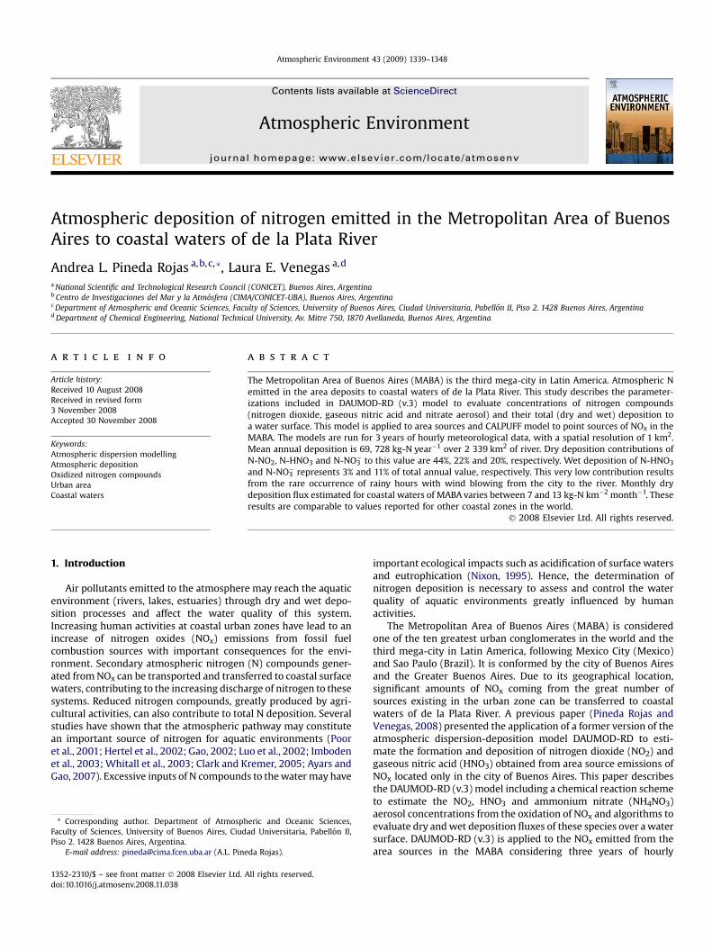
Fig. 1. Schematic illustration of the chemical transformations included in the DAUMOD-RDradical; ROG, reactive organic gases; HNO3, gaseous nitric acid; NH3, gaseous ammonia; NH

application of complex numerical tools not possible, and simpleurban background pollution models become an acceptable alter-native. The performance of the model in estimating air pollutantconcentrations has been evaluated in previous papers (Mazzeo andVenegas, 1991; Venegas and Mazzeo, 2002, 2006). Results showthat the ability of the DAUMOD model to estimate pollutantconcentrations in short averaging time (hourly and daily) is goodand it improves when estimating values in long averaging time(monthly and annual).

In order to estimate the transfer of nitrogen from the NOx

emitted in the urban area to coastal waters, parameterizations offormation of secondary oxidized nitrogen compounds (NO2,gaseous HNO3 and NH4NO3 aerosol) and their dry and wetdeposition to a water surface, are included in the model. Nitricacid may also be combined with sea salt particles to form sodiumnitrate. However, the main sources of sodium are the sea spraydroplets greatly produced at the breaking zones, so this reactionmight be important in marine environments (Pryor and Sør-ensen, 2000; de Leeuw et al., 2001). Despite MABA not being ina marine environment, a preliminary study (Bogo et al., 2003)revealed the presence of sodium in the atmosphere. That studyrecommended that this possible marine characteristic in theatmosphere of Buenos Aires should be investigated in a moresystematic study. Since no further results are available atpresent, the formation of sodium nitrate is not included in themodel.

The model assumes that pollutants are dispersed in the domainbefore being removed from the atmosphere; therefore, depositionover land before reaching the shoreline is not evaluated.

2.2. Chemical reactions

The scheme of chemical transformations included in the DAU-MOD-RD (v.3) model is briefly illustrated in Fig. 1. The firstconservative assumption is that NOx emitted to the atmosphere isall transformed to NO2. In presence of solar light, NO2 is oxidized toHNO3 according to the reaction:

NO2 þ OHþM/HNO3 þM (4)

and organic nitrates (RNO3). The HNO3 can then react with gaseousammonia (NH3) present in the atmosphere to form NH4NO3 aerosol(solid or aqueous) through a reversible process:

NH3ðgÞ þHNO3ðgÞ4NH4NO3 (5)

2.2.1. Gas phaseIn the model, the mechanisms through which NO2 is lost and

HNO3 is formed are considered as pseudo-first-order reactions, andthe concentrations of these species following the oxidation of NOx

can therefore be calculated as (Scire et al., 2000):

½NO2� ¼ ½NOx�expð�k1Dt=100Þ (6)

½HNO3�i¼ ½NOx�½1� expð�k2Dt=100Þ� (7)

NH4NO3NH3HNO3

RNO3

(v.3) model. NOx, nitrogen oxides; NO2, nitrogen dioxide; O3, ozone; HO2, hydroperoxyl

4NO3, ammonium nitrate aerosol; RNO3, organic nitrates.

A.L. Pineda Rojas, L.E. Venegas / Atmospheric Environment 43 (2009) 1339–1348 1341

where the subscript i denotes ‘‘initial’’ concentration of HNO3 [i.e.,after reaction (4) and before reaction (5)], Dt is the model time step(¼1 h) and [NOx] is the concentration (ppm) of NOx (expressed asNO2) before reacting [estimated by Eqs. (1) and (3)].

The reaction constants for the loss of NO2 (k1) and the formationof HNO3 (k2), can be estimated by the expressions (Scire et al.,2000):

k1 ¼ 1206½O3�1:5S�1:41½NOx��0:329m (8)

k2 ¼ 1262½O3�1:45S�1:34½NOx��0:122m (9)

where [O3] is the ozone background concentration (ppm), S is anatmospheric stability index [that varies between 2–6 according tothe Pasquill–Gifford–Turner classification (Gifford, 1976)], and½NOx�m is the vertically averaged NOx concentration (ppm) withinthe pollutant plume, which can be obtained using Eq. (1) as:

Cm ¼1h

Z h

0Cðx; zÞ dz ¼ 1

h

Z h

0Cðx;0Þ

X6

j¼0

Ajðz=hÞjdz

¼ Cðx;0ÞX6

j¼0

�Aj=ðjþ 1Þ

�(10)

At night, due to the relatively low concentration of the OH radical,NOx oxidation rates are lower than typical diurnal rates andconstant values of k1 ¼ k2 ¼ 2.0% h�1 are considered (Scire et al.,2000).

2.2.2. Aerosol phaseAccording to reaction (5), part of HNO3 formed from the

oxidation of NOx [Eq. (7)] will be converted to NH4NO3 aerosol andthe rest will remain as gaseous HNO3. The fraction (g) of ammo-nium nitrate aerosol in equilibrium with gaseous HNO3 and NH3, iscalculated as:

g ¼ ½NH4NO3�=½NO3�T (11)

where [NH4NO3] is the ammonium nitrate equilibrium concentra-tion and [NO3]T is the total nitrate concentration. In DAUMOD-RD(v.3) model, [NO3]T ¼ [HNO3]i is considered. Based on equilibriumconsiderations and assuming conservation of total nitrate and totalammonia concentrations, [NH4NO3] is obtained as a function ofthese parameters and the equilibrium constant. It is considered thattotal NH3 concentration is given by its background value. If noobservations of hourly background ammonia concentration areavailable, monthly mean values can be used (Scire et al., 2000). Theequilibrium constant is a nonlinear function of temperature andrelative humidity and is estimated through a double linear inter-polation algorithm on these variables following the relationshipsobtained by Stelson and Seinfeld (1982). Finally, gaseous HNO3 andNH4NO3 aerosol concentrations are estimated as:

½HNO3� ¼ ð1� gÞ½HNO3�i (12)

½NH4NO3� ¼ g½HNO3�i (13)

2.3. Depositions module

2.3.1. Wet depositionConsidering that the species is irreversibly soluble and that the

size of drops does not vary with height, the wet deposition flux (Fw)can be estimated according to (Seinfeld and Pandis, 1998):

Fw ¼ LhCm (14)

where L is the scavenging coefficient (s�1), h is calculated from Eq.(2) and Cm is the vertically averaged pollutant concentration beforethe wet removal process, computed from Eq. (10). The scavengingcoefficient can be parameterized in terms of the precipitationintensity (p0) by the following expression (Levine and Schwartz,1982; Mircea et al., 2000; Scire et al., 2000; Sportisse and du Bois,2002):

L ¼ lðp0=p1Þ (15)

where p1 is a reference value (¼1 mm h�1) and l is a washoutcoefficient (s�1) that depends on the species. Due to the low solu-bility of nitrogen dioxide in water, the removal of NO2 by precipi-tation can be assumed negligible (Lee and Schwartz, 1981; Seinfeldand Pandis, 1998). In DAUMOD-RD (v.3), l ¼ 0 for nitrogen dioxide,6.0E-05 s�1 for gaseous nitric acid and 1.0E-04 s�1 for nitrateaerosol (Scire et al., 2000) are considered.

The air concentration of each species remaining after the rainscavenging (C0) is estimated by the expression:

C0ðx; zÞ ¼ Cðx; zÞexpð � LDtÞ (16)

where C represents the species concentration before the wetremoval [given by Eq. (12) for gaseous HNO3 and Eq. (13) forNH4NO3 aerosol].

2.3.2. Dry deposition over waterThe dry deposition flux (Fd) is estimated by:

Fd ¼ vdC0ðx;0Þ (17)

where vd is the deposition velocity (cm s�1) of the species andC0(x,0) is given by Eq. (16) [note that in absence of precipitation, Eq.(16) gives C0(x,0) ¼ C(x,0)]. The deposition velocities of gaseousspecies (vdg) and aerosol (vdp) are parameterized applying theresistance method. Based on an assumption of steady-state depo-sition flux conditions, these deposition velocities can be expressedas (Seinfeld and Pandis, 1998):

vdg ¼�

ra þ rdg þ rw

��1(18)

vdp ¼�

ra þ rdp þ rardpvs

��1þvs (19)

where ra is the aerodynamic resistance (s cm�1), rdg and rdp are thequasi-laminar layer resistances (s cm�1) for gaseous and aerosolspecies, respectively, rw is the water surface resistance (s cm�1) andvs is the aerosol gravitational settling velocity (cm s�1).

2.3.2.1. Aerodynamic resistance (ra). This resistance represents theeffect of turbulent transport of species through the atmosphericsurface layer and does not depend on the type of species (gas oraerosol) but on the atmospheric conditions. It is estimated followingthe Monin–Obukhov theory as (Seinfeld and Pandis, 1998):

ra ¼ ½lnðzr=z0Þ � 4Hðzr=LÞ�=ðku*Þ (20)

where zr is a reference level (zr ¼ 1 m), L is the Monin–Obukhovlength (m) and 4H is a stability correction term (Wieringa, 1980;Gryning et al., 1987):

4Hðzr=LÞ ¼��9:2zr=L zr=L � 02 ln½ðhr þ 1Þ=ðh0 þ 1Þ� zr=L < 0

(21)

with hr ¼ (1–13zr/L)1/2 and h0 ¼ (1–13z0/L)1/2. The water surfaceroughness length (z0) (m) is evaluated considering the wind speed(u) (m s�1) at 10 m height (Hosker, 1974):

A.L. Pineda Rojas, L.E. Venegas / Atmospheric Environment 43 (2009) 1339–13481342

z0 ¼ 2:0E� 06u2:5 (22)

CBA

GBA

de la Plata River

10 km

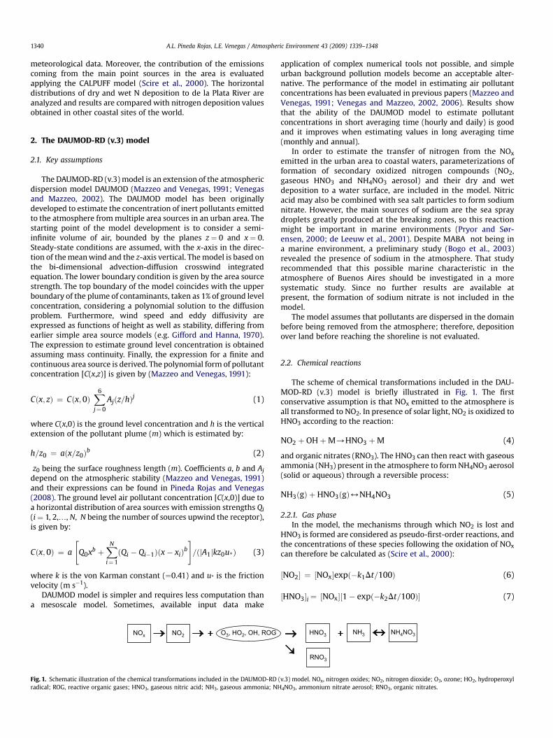
Fig. 2. Area of study: Metropolitan Area of Buenos Aires (MABA) composed by the cityof Buenos Aires (CBA) and 24 districts from the Greater Buenos Aires (GBA); JorgeNewbery Domestic Airport (downward aeroplane symbol) and Ministro Pistarini(Ezeiza) International Airport (upward aeroplane symbol); thermal power plants (:);oil company (6) and surface of de la Plata River in front of MABA considered forcalculations.

2.3.2.2. Quasi-laminar layer resistance for gases (rdg). This resis-tance includes the effects of molecular diffusion of species throughthis thin layer and is calculated in terms of the Schmidt number(Sc ¼ na/n, where na is the air kinematic viscosity and n is thepollutant molecular diffusivity in air) by:

rdg ¼ d1Scd2=ðku*Þ (23)

d1 and d2 are empirical parameters assumed to be 2 and 2/3,respectively (Scire et al., 2000).

2.3.2.3. Quasi-laminar layer resistance for aerosol particles (rdp). Inthe case of aerosols, the quasi-laminar layer resistance accounts forBrownian diffusion, inertial impaction and interception processes.This resistance can be parameterized as a function of the Schmidtnumber and the Stokes number (St) as:

rdp ¼h�

Sc�2=3 þ 10�3=St�

u*

i�1(24)

The Stokes number is a measure of the likelihood of impaction ofthe particle and is given by (Seinfeld and Pandis, 1998):

St ¼ vsu2*=ðgnaÞ (25)

where g is the acceleration due to gravity (9.8 m s�2).

2.3.2.4. Gravitational settling velocity (vs). The gravitational settlingvelocity of aerosol particles is given by the Stokes equation:

vs ¼ rpd2pgCc=ð18maÞ (26)

where rp is the particle density (g cm�3), ma is the air dynamicviscosity (1.81E-04 g cm�1 s�1), dp is the particle diameter (mm) andCc is the Cunningham correction factor for small particles, given by:

Cc ¼ 1þ�2c=dp

��a1 þ a2exp

��a3dp=c

��(27)

c being the mean free path of particles (¼6.53E-06 cm) anda1 ¼1.257, a2 ¼ 0.40 and a3 ¼ 0.55. The particle diffusivity in air (n)included in the Schmidt number is a function of the particle sizeand can be estimated as:

n ¼ d3Cc=�3pmadp

�(28)

where d3 is a constant (¼4.045E-14).

2.3.2.5. Water surface resistance (rw). Finally, the water surfaceresistance for gaseous species is calculated from (Slinn et al., 1978):

rw ¼ H=ða*d4u*Þ (29)

where H is the Henry’s Law constant (i.e., ratio of gas to liquid phasepollutant concentration), a* is a factor related to the pollutantdissociation in the aqueous phase and d4 is a constant (¼4.8E-04).

2.4. Inclusion of particle size

According to Eqs. (24)–(28), the quasi-laminar layer resistancefor aerosols (rdp) and the gravitational settling velocity (vs) dependon the particle size (dp). To include these dependences in themodel, a log-normal distribution with typical parameters fornitrate aerosol [geometric mean diameter: dp ¼ 0.48 mm,geometric standard deviation: sp ¼ 2.0 mm (Scire et al., 2000)] isconsidered. The distribution is divided into Nint particle sizeintervals, for which values of rdp and vs are evaluated as a function

of the interval mean diameter (Nint ¼ 9 is considered). Then, an‘‘effective’’ deposition velocity (vdpe) for each interval j of thedistribution is obtained:

vdpeðjÞ ¼hra þ rdpðjÞ þ rardpðjÞvsðjÞ

i�1þ vsðjÞ (30)

and the ‘‘total’’ deposition velocity (vdp) is therefore calculated asthe weighted average of the effective deposition velocities:

vdp ¼XNint

j¼1

vdpeðjÞfpðjÞ (31)

where fp(j) is the fraction of aerosol mass with diameters within theinterval j.

3. NOx emission data

The Metropolitan Area of Buenos Aires (MABA) has 11. 460.575 inhabitants within an extension of 3 827 km2 (see Fig. 2).NOx emission data belong to a recently developed (Pineda Rojaset al., 2007) high spatial resolution (1 km2) emission inventory.Emission sources are classified into area and point sources. Areasources include road transport (cars, tracks and buses), resi-dential, commercial and small industry activities and aircrafts atthe Domestic and International airports. Moreover, the stacks offour thermal power plants and a large oil company (shown inFig. 2) are considered as the main point sources located near thecoast.

Table 1 includes the annual NOx emission for each sourcecategory considered in the MABA. Area sources account for 67% (66,823 ton-NOx year�1) of NOx annual emissions in the MABA. Themain contribution to this value comes from vehicles (81%). Resi-dential, commercial and small industry activities representa contribution of 18% and aircrafts account for around 1% of totalarea source NOx emission.

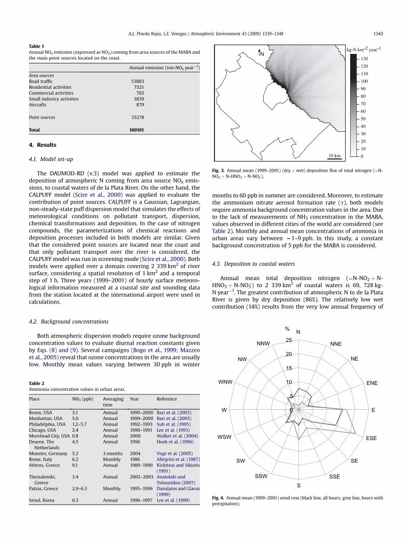
Table 1Annual NOx emission (expressed as NO2) coming from area sources of the MABA andthe main point sources located on the coast.

Annual emission (ton-NOx year�1)

Area sourcesRoad traffic 53883Residential activities 7521Commercial activities 702Small industry activities 3839Aircrafts 879

Point sources 33278

Total 100101

0

10

20

30

40

50

60

70

80

90

100

110

120

130

10 km

kg-N km-2 year-1

Fig. 3. Annual mean (1999–2001) (dry þwet) deposition flux of total nitrogen (¼N-NO2 þ N-HNO3 þ N-NO3

�).

A.L. Pineda Rojas, L.E. Venegas / Atmospheric Environment 43 (2009) 1339–1348 1343

4. Results

4.1. Model set-up

The DAUMOD-RD (v.3) model was applied to estimate thedeposition of atmospheric N coming from area source NOx emis-sions, to coastal waters of de la Plata River. On the other hand, theCALPUFF model (Scire et al., 2000) was applied to evaluate thecontribution of point sources. CALPUFF is a Gaussian, Lagrangian,non-steady-state puff dispersion model that simulates the effects ofmeteorological conditions on pollutant transport, dispersion,chemical transformations and deposition. In the case of nitrogencompounds, the parameterizations of chemical reactions anddeposition processes included in both models are similar. Giventhat the considered point sources are located near the coast andthat only pollutant transport over the river is considered, theCALPUFF model was run in screening mode (Scire et al., 2000). Bothmodels were applied over a domain covering 2 339 km2 of riversurface, considering a spatial resolution of 1 km2 and a temporalstep of 1 h. Three years (1999–2001) of hourly surface meteoro-logical information measured at a coastal site and sounding datafrom the station located at the international airport were used incalculations.

20

25N

NNE

NENW

NNW

%

4.2. Background concentrations

Both atmospheric dispersion models require ozone backgroundconcentration values to evaluate diurnal reaction constants givenby Eqs. (8) and (9). Several campaigns (Bogo et al., 1999; Mazzeoet al., 2005) reveal that ozone concentrations in the area are usuallylow. Monthly mean values varying between 30 ppb in winter

Table 2Ammonia concentration values in urban areas.

Place NH3 (ppb) Averagingtime

Year Reference

Bronx, USA 3.1 Annual 1999–2000 Bari et al. (2003)Manhattan, USA 5.0 Annual 1999–2000 Bari et al. (2003)Philadelphia, USA 1.2–5.7 Annual 1992–1993 Suh et al. (1995)Chicago, USA 2.4 Annual 1990–1991 Lee et al. (1993)Morehead City, USA 0.8 Annual 2000 Walker et al. (2004)Deurne, The

Netherlands4.5 Annual 1996 Hoek et al. (1996)

Munster, Germany 5.2 3 months 2004 Vogt et al. (2005)Rome, Italy 6.2 Monthly 1986 Allegrini et al. (1987)Athens, Greece 9.1 Annual 1989–1990 Kirkitsos and Sikiotis

(1991)Thessaloniki,

Greece3.4 Annual 2002–2003 Anatolaki and

Tsitouridou (2007)Patras, Greece 2.9–6.3 Monthly 1995–1996 Danalatos and Glavas

(1999)Seoul, Korea 6.3 Annual 1996–1997 Lee et al. (1999)

months to 60 ppb in summer are considered. Moreover, to estimatethe ammonium nitrate aerosol formation rate (g), both modelsrequire ammonia background concentration values in the area. Dueto the lack of measurements of NH3 concentration in the MABA,values observed in different cities of the world are considered (seeTable 2). Monthly and annual mean concentrations of ammonia inurban areas vary between w1–9 ppb. In this study, a constantbackground concentration of 5 ppb for the MABA is considered.

4.3. Deposition to coastal waters

Annual mean total deposition nitrogen (¼N-NO2 þ N-HNO3 þ N-NO3

�) to 2 339 km2 of coastal waters is 69, 728 kg-N year�1. The greatest contribution of atmospheric N to de la PlataRiver is given by dry deposition (86%). The relatively low wetcontribution (14%) results from the very low annual frequency of

0

5

10

15

ENE

E

ESE

SE

SSES

SSW

SW

WSW

W

WNW

Fig. 4. Annual mean (1999–2001) wind rose (black line, all hours; grey line, hours withprecipitation).

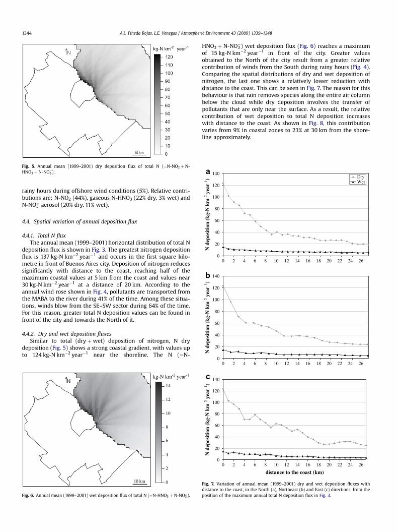
Fig. 5. Annual mean (1999–2001) dry deposition flux of total N (¼N-NO2 þ N-HNO3 þ N-NO3

�).

100

120

140

km

-2 y

ear-1

) DryWet

a

A.L. Pineda Rojas, L.E. Venegas / Atmospheric Environment 43 (2009) 1339–13481344

rainy hours during offshore wind conditions (5%). Relative contri-butions are: N-NO2 (44%), gaseous N-HNO3 (22% dry, 3% wet) andN-NO3

� aerosol (20% dry, 11% wet).

0

20

40

60

80N

dep

osit

ion

(kg-

N

0

20

40

60

80

100

120

140

N d

epos

itio

n (k

g-N

km

-2 y

ear-1

)

0 2 4 6 8 10 12 14 16 18 20 22 24 26

b

4.4. Spatial variation of annual deposition flux

4.4.1. Total N fluxThe annual mean (1999–2001) horizontal distribution of total N

deposition flux is shown in Fig. 3. The greatest nitrogen depositionflux is 137 kg-N km�2 year�1 and occurs in the first square kilo-metre in front of Buenos Aires city. Deposition of nitrogen reducessignificantly with distance to the coast, reaching half of themaximum coastal values at 5 km from the coast and values near30 kg-N km�2 year�1 at a distance of 20 km. According to theannual wind rose shown in Fig. 4, pollutants are transported fromthe MABA to the river during 41% of the time. Among these situa-tions, winds blow from the SE–SW sector during 64% of the time.For this reason, greater total N deposition values can be found infront of the city and towards the North of it.

4.4.2. Dry and wet deposition fluxesSimilar to total (dry þwet) deposition of nitrogen, N dry

deposition (Fig. 5) shows a strong coastal gradient, with values upto 124 kg-N km�2 year�1 near the shoreline. The N (¼N-

0

2

4

6

8

10

12

14

10 km

kg-N km-2 year-1

Fig. 6. Annual mean (1999–2001) wet deposition flux of total N (¼N-HNO3 þ N-NO3�).

HNO3 þ N-NO3�) wet deposition flux (Fig. 6) reaches a maximum

of 15 kg-N km�2 year�1 in front of the city. Greater valuesobtained to the North of the city result from a greater relativecontribution of winds from the South during rainy hours (Fig. 4).Comparing the spatial distributions of dry and wet deposition ofnitrogen, the last one shows a relatively lower reduction withdistance to the coast. This can be seen in Fig. 7. The reason for thisbehaviour is that rain removes species along the entire air columnbelow the cloud while dry deposition involves the transfer ofpollutants that are only near the surface. As a result, the relativecontribution of wet deposition to total N deposition increaseswith distance to the coast. As shown in Fig. 8, this contributionvaries from 9% in coastal zones to 23% at 30 km from the shore-line approximately.

0

20

40

60

80

100

120

140

0 2 4 6 8 10 12 14 16 18 20 22 24 26

0 2 4 6 8 10 12 14 16 18 20 22 24 26

distance to the coast (km)

N d

epos

itio

n (k

g-N

km

-2 y

ear-1

)

c

Fig. 7. Variation of annual mean (1999–2001) dry and wet deposition fluxes withdistance to the coast, in the North (a), Northeast (b) and East (c) directions, from theposition of the maximum annual total N deposition flux in Fig. 3.

8

10

12

14

16

18

20

22

%

10 km

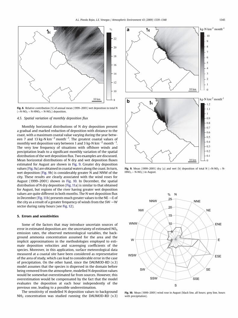
Fig. 8. Relative contribution (%) of annual mean (1999–2001) wet deposition to total N(¼N-NO2 þ N-HNO3 þ N-NO3

�) deposition.

0

1

2

3

4

5

6

7

8

9

10

b

kg-N km-2 month-1

1

0

0.1

0.2

0.3

0.4

0.5

0.6

0.7

0.8

0.9

1.1

1.2

10 km

kg-N km-2 month-1

10 km

a

Fig. 9. Mean (1999–2001) dry (a) and wet (b) deposition of total N (¼N-NO2 þ N-HNO3 þ N-NO3

�) in August.

20

25N

NNENNW

%

A.L. Pineda Rojas, L.E. Venegas / Atmospheric Environment 43 (2009) 1339–1348 1345

4.5. Spatial variation of monthly deposition flux

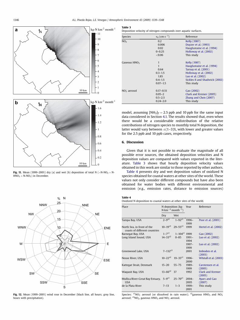
Monthly horizontal distributions of N dry deposition presenta gradual and marked reduction of deposition with distance to thecoast, with a maximum coastal value varying during the year betw-een 7 and 13 kg-N km�2 month�1. The greatest coastal values ofmonthly wet deposition vary between 1 and 3 kg-N km�2 month�1.The very low frequency of situations with offshore winds andprecipitation leads to a significant monthly variation of the spatialdistribution of the wet deposition flux. Two examples are discussed.Mean horizontal distributions of N dry and wet deposition fluxesestimated for August are shown in Fig. 9. Greater dry depositionvalues (Fig. 9a) are obtained in coastal waters along the coast. In turn,wet deposition (Fig. 9b) is considerably greater N and NNW of thecity. These results are clearly associated with the wind roses forAugust (1999–2001) shown in Fig. 10. In December, the spatialdistribution of N dry deposition (Fig. 11a) is similar to that obtainedfor August, but regions of the river having greater wet depositionvalues are quite different in both months. The N wet deposition fluxin December (Fig.11b) presents much greater values to the NE/E ofthe city as a result of a greater frequency of winds from the SW/Wsector during rainy hours (see Fig. 12).

0

5

10

15NE

ENE

E

ESE

SE

SSE

S

SSW

SW

WSW

W

WNW

NW

Fig. 10. Mean (1999–2001) wind rose in August (black line, all hours; grey line, hourswith precipitation).

5. Errors and sensitivities

Some of the factors that may introduce uncertain sources oferror in estimated deposition are: the uncertainty of estimated NOx

emission rates, the observed meteorological variables, the back-ground ammonia concentration assumed for the area and theimplicit approximations in the methodologies employed to esti-mate deposition velocities and scavenging coefficients of thespecies. Moreover, in this application, surface meteorological datameasured at a coastal site have been considered as representativeof the area of study, which can lead to considerable error in the caseof precipitation. On the other hand, since the DAUMOD-RD (v.3)model assumes that the species is dispersed in the domain beforebeing removed from the atmosphere, modelled N deposition valueswould be somewhat overestimated far from sources. However, thisoverestimation would be compensated by the fact that the modelevaluates the deposition at each hour independently of theprevious one, leading to a possible underestimation.

The sensitivity of modelled N deposition values to backgroundNH3 concentration was studied running the DAUMOD-RD (v.3)

0

5

10

15

20

25N

NNE

NE

ENE

E

ESE

SE

SSES

SSW

SW

WSW

W

WNW

NW

NNW

%

Fig. 12. Mean (1999–2001) wind rose in December (black line, all hours; grey line,hours with precipitation).

Table 3Deposition velocity of nitrogen compounds over aquatic surfaces.

Species vd (cm s�1) Reference

NO2 0.2 Kelly (1987)0.006 Duyzer et al. (1993)0.02 Hauglustaine et al. (1994)

0–0.25 Holloway et al. (2002)<0.06 This study

Gaseous HNO3 1 Kelly (1987)1 Hauglustaine et al. (1994)0.64 Tarnay et al. (2001)

0.3–1.5 Holloway et al. (2002)1.85 Luo et al. (2002)

0.4–1.5 Sickles II and Shadwick (2002)0.07–1.5 This study

NO3� aerosol 0.17–0.51 Gao (2002)

0.05–2 Clark and Kremer (2005)0.5–2.5 Zhang and Chen (2007)0.24–2.0 This study

0

1

2

3

4

5

6

7

8

9

10

11a

10 km

kg-N km-2 month-1

0

0.2

0.4

0.6

0.8

1

1.2

1.4

1.6

10 km

kg-N km-2 month-1b

Fig. 11. Mean (1999–2001) dry (a) and wet (b) deposition of total N (¼N-NO2 þ N-HNO3 þ N-NO3

�) in December.

A.L. Pineda Rojas, L.E. Venegas / Atmospheric Environment 43 (2009) 1339–13481346

model, assuming [NH3]T ¼ 2.5 ppb and 10 ppb for the same inputdata considered in Section 4.1. The results showed that, even whenthere would be a considerable redistribution of the relativecontributions of nitrogen species to monthly total N deposition, thelatter would vary between �(1–3)%, with lower and greater valuesfor the 2.5 ppb and 10 ppb cases, respectively.

6. Discussion

Given that it is not possible to evaluate the magnitude of allpossible error sources, the obtained deposition velocities and Ndeposition values are compared with values reported in the liter-ature. Table 3 shows that hourly deposition velocity valuesobtained in this work are similar to those reported by other authors.

Table 4 presents dry and wet deposition values of oxidized Nspecies obtained for coastal waters at other sites of the world. Thesevalues not only consider different compounds but have also beenobtained for water bodies with different environmental andemission (e.g., emission rates, distance to emission sources)

Table 4Oxidized N deposition to coastal waters at other sites of the world.

Place N deposition (kg-N km�2 month�1)

Year Reference

Dry Wet

Tampa Bay, USA 2–9s2 1–92s1 1996–1999

Poor et al. (2001)

North Sea, in front of thecoasts of different countries

10–19s3 29–55s3 1999 Hertel et al. (2002)

Barnegat Bay, USA 1–7s1 1–104s1 1999 Gao (2002)Long Island Sound, USA 14–33s2 0–85 1991–

1994Luo et al. (2002)

1997–1999

Luo et al. (2002)

Greenwood Lake, USA 7–132s3 2001 Imboden et al.(2003)

Neuse River, USA 10–22s2 19–35s1 1996–2000

Whitall et al. (2003)

Kattegat Strait, Denmark 15–20 55–75 1989–1999

Carstensen et al.(2005)

Waquoit Bay, USA 13–66s2 37 1992 Clark and Kremer(2005)

Mullica River-Great Bay Estuary,USA

5–9s1 25–70s1 2004–2005

Ayars and Gao(2007)

de la Plata River 7–13 1–3 1999–2001

This study

Species: s1NO3� aerosol (or dissolved in rain water); s2gaseous HNO3 and NO3

�

aerosol; s3NO2, gaseous HNO3 and NO3� aerosol.

A.L. Pineda Rojas, L.E. Venegas / Atmospheric Environment 43 (2009) 1339–1348 1347

conditions. However, maximum coastal values of monthly N drydeposition estimated in this study (7–13 kg-N km�2 month�1) areconsistent with other reported data. On the other hand, Table 4shows that monthly wet deposition can vary significantly from nearzero to 100 kg-N km�2 month�1. The estimated monthly wetdeposition of oxidized nitrogen to de la Plata River results too smalldue to the very few cases of favourable situations for wet depositionregistered in the area.

It is worth noting that reduced nitrogen compounds (NHx) couldalso contribute significantly to total N deposition. While NHx maybe considered to be N returning to the water body (Hertel et al.,2002; Clark and Kremer, 2005), local sources could still makea substantial contribution. Unfortunately, at present, no ammoniaemission inventory for the MABA is available so as to include theanthropogenic contribution of NHx on calculations.

7. Conclusions

The DAUMOD-RD (v.3) model was developed in order to eval-uate air concentrations of nitrogen compounds generated from NOx

emissions and total deposition of these species over a water surface,when emissions come from a great number of area sources ina coastal city. This model was applied to area sources in theMetropolitan Area of Buenos Aires and the CALPUFF model to mainpoint sources located near the coast, to estimate the N deposition tocoastal waters of de la Plata River. Both models were run consid-ering a spatial resolution of 1 km2, 3 years of hourly meteorologicalinformation and high resolution NOx emission data.

Annual mean deposition of total N (¼N-NO2 þ N-HNO3 þ N-NO3�) to waters (2 339 km2) of the river is 69, 728 kg-N year�1. Dry

deposition contributions of N-NO2, N-HNO3 and N-NO3� to this

value are 44%, 22% and 20%, respectively. Wet deposition of N-HNO3

and N-NO3� represents 3% and 11%, respectively. Maximum monthly

dry deposition flux obtained for de la Plata River varies between 7–13 kg-N km�2 month�1. These results are comparable to thoseobtained by other authors for coastal waters at different parts of theworld. However, estimated maximum wet deposition flux (1–3 kg-N km�2 month�1) is near one order of magnitude lower than valuesreported for other coastal zones. The low contribution of wetdeposition is the result of the very low frequency (5%) of hours withprecipitation during offshore wind conditions.

Acknowledgements

This work has been partially supported by Projects UBACyTX060 and CONICET-PIP 6169. The authors wish to thank theNational Meteorological Service of Argentina for providing mete-orological data. The authors are grateful to unknown reviewers fortheir helpful comments and suggestions.

References

Allegrini, I., DeSantis, F., DiPalo, V., Febo, A., Perrino, C., Possanzini, M., 1987. Annulardenuder method for sampling reactive gases and aerosols in the atmosphere.Science of the Total Environment 67, 1–16.

Anatolaki, Ch, Tsitouridou, R., 2007. Atmospheric deposition of nitrogen, sulfur andchloride in Thessaloniki, Greece. Atmospheric Research 85 (3–4), 413–428.

Ayars, J., Gao, Y., 2007. Atmospheric nitrogen deposition to the Mullica River-GreatBay Estuary. Marine Environmental Research 64, 590–600.

Bari, A., Ferraro, V., Wilson, L.R., Luttinger, D., Husain, L., 2003. Measurements ofgaseous HONO, HNO3, SO2, HCl, NH3, particulate sulfate and PM2.5 in New York,NY. Atmospheric Environment 37, 2825–2835.

Bogo, H., Negri, R.M., San Roman, E., 1999. Continuous measurement of gaseouspollutants in Buenos Aires City. Atmospheric Environment 33, 2587–2598.

Bogo, H., Otero, M., Castro, P., Azafran, M.J., Kreiner, A., Calvo, E., Negri, R.M., 2003.Study of atmospheric particulate matter in Buenos Aires city. AtmosphericEnvironment 37, 1135–1147.

Carstensen, J., Frohn, L.M., Hasager, C.B., Gustafsson, B.G., 2005. Summer algalblooms in a coastal ecosystem: the role of atmospheric deposition versusentrainment fluxes. Estuarine. Coastal and Shelf Science 62, 595–608.

Clark, H., Kremer, J.N., 2005. Estimating direct and episodic atmospheric nitrogendeposition to a coastal waterbody. Marine Environmental Research 59,349–366.

Danalatos, D., Glavas, S., 1999. Gas phase nitric acid, ammonia and related partic-ulate matter at a Mediterranean coastal site, Patras, Greece. AtmosphericEnvironment 33, 3417–3425.

Duyzer, J.H., Verhagen, H., Westrate, J., 1993. Dry deposition of ozone, nitrogendioxide and ammonia to seawater. IMW-R 93/131, TNO Institute of Environ-mental Sciences, Delft, The Netherlands.

Gao, Y., 2002. Atmospheric nitrogen deposition to Barnegat Bay. AtmosphericEnvironment 36, 5783–5794.

Gifford, F.A., 1976. Turbulent diffusion typing schemes: a review. Nuclear Safety 17(1), 25–43.

Gifford, F.A., Hanna, S.R., 1970. Urban Air Pollution Modeling. Meeting Int. Union ofAir Pollut. Prev. Assoc. Washington.

Gryning, S.E., Footslog, A.A.M., Irwin, J.S., Silvertsen, B., 1987. Applied dispersionmodelling based on meteorological scaling parameters. Atmospheric Environ-ment 21, 79–89.

Hauglustaine, D.A., Granier, C., Brasseur, G.P., Megie, G., 1994. The importance ofatmospheric chemistry in the calculation of radiative forcing on the climatesystem. Journal of Geophysical Research 99, 1173–1186.

Hertel, O., Ambelas Skjøth, C., Frohn, L.M., Vignati, E., Frydendall, J., de Leeuw, G.,Schwarz, U., Reis, S., 2002. Assessment of the atmospheric nitrogen and sulphurinputs into the North Sea using a Lagrangian model. Physics and Chemistry ofthe Earth 27, 1507–1515.

Hoek, G., Mennen, M.G., Allen, G.A., Hofschreuder, P., Meulen, T.V., 1996. Concen-trations of acidic air pollutants in the Netherlands. Atmospheric Environment30, 3141–3150.

Holloway, T., Levy, H., Carmichael, G., 2002. Transfer of reactive nitrogen in Asia:development and evaluation of a source-receptor model. Atmospheric Envi-ronment 36, 4251–4264.

Hosker, R.P., 1974. A comparison of estimation procedures for overwater plumedispersion. Proceedings of the Symposium on Atmospheric Diffusion and AirPollution. American Meteorological Society, Boston, MA. 281–288.

Imboden, A., Christoforou, S., Salmon, L.G., 2003. Determination of atmosphericnitrogen input to Lake Greenwood, South Carolina: Part 2dgaseous measure-ments and modeling. Journal of Air and Waste Management Association 53,1499–1508.

Kelly, N.A., 1987. The photochemical formation and fate of nitric acid in theMetropolitan Detroit Area: ambient, captive-air irradiation and modelingresults. Atmospheric Environment 21, 2163–2177.

Kirkitsos, F.D., Sikiotis, D., 1991. Nitric acid, ammonia and particulate nitrates,sulfates and ammonium in the atmosphere of Athens. Ecistics 348–349,156–163.

Lee, Y., Schwartz, S.E., 1981. Evaluation of the rate of uptake of nitrogen dioxide byatmospheric and surface liquid water. Journal of Geophysical Research 86 (C12),11971–11983.

Lee, H.S., Wadden, R.A., Scheff, P.A., 1993. Measurement and evaluation of acid airpollutants in Chicago using an annular denuder system. Atmospheric Envi-ronment 27A, 543–553.

Lee, H.S., Kang, C.-M., Kang, B.-W., Kim, H.-K., 1999. Seasonal variations of acidic airpollutants in Seoul, South Korea. Atmospheric Environment 33, 3143–3152.

de Leeuw, G., Cohen, L., Frohn, L.M., Geernaert, G., Hertel, O., Jensen, B., Jickells, T.,Klein, L., Kunz, G., Lund, S., Moerman, M., Muller, F., Pedersen, B., Salzen, K.,Schluenzen, H., Schulz, M., Skjøth, C.A., Sørensen, L.L., Spokes, L., Tamm, S.,Vignati, E., 2001. Atmospheric input of nitrogen in the North Sea: ANICE ProjectOverview. Continental Shelf Research 21, 2073–2094.

Levine, S.Z., Schwartz, S.E., 1982. In-cloud and below-cloud scavenging of nitric acidvapor. Atmospheric Environment 16 (7), 1725–1734.

Luo, Y., Yang, X., Carley, R.J., Perkins, C., 2002. Atmospheric deposition of nitrogenalong the Connecticut coastline of Long Island Sound: a decade of measure-ments. Atmospheric Environment 36, 4517–4528.

Mazzeo, N.A., Venegas, L.E., 1991. Air pollution model for an urban area. Atmo-spheric Research 26, 165–179.

Mazzeo, N.A., Venegas, L.E., Choren, H., 2005. Analysis of NO, NO2, O3 and NOxconcentrations measured at a green area of Buenos Aires City during winter-time. Atmospheric Environment 39, 3055–3068.

Mircea, M., Stefan, S., Fuzzi, S., 2000. Precipitation scavenging coefficient: influenceof measured aerosol and raindrop size distributions. Atmospheric Environment34, 5169–5174.

Nixon, S.W., 1995. Coastal marine eutrophication: A definition, social causes, andfuture concerns. Ophelia 41, 199–219.

Pineda Rojas, A.L., Venegas, L.E., 2008. Dry and wet deposition of nitrogen emittedin Buenos Aires city to waters of de la Plata River. Water, Air, & Soil Pollution193, 175–188.

Pineda Rojas, A.L., Venegas, L.E., Mazzeo, N.A., 2007. Emission inventory of carbonmonoxide and nitrogen oxides for area sources at Buenos Aires Metropolitan Area(Argentina). Proceedings of the 6th International Conference on Urban Air Quality,Emission measurements and modelling sessions, Cyprus, CD-ROM, 35–38.

Poor, N., Pribble, R., Greening, H., 2001. Direct wet and dry deposition of ammonia,nitric acid, ammonium and nitrate to the Tampa Bay Estuary, FL, USA. Atmo-spheric Environment 35, 3947–3955.

A.L. Pineda Rojas, L.E. Venegas / Atmospheric Environment 43 (2009) 1339–13481348

Pryor, S.C., Sørensen, L.L., 2000. Nitric Acid-sea salt reactions: implications fornitrogen deposition to water surfaces. Journal of Applied Meteorology 39,725–731.

Scire, J.S., Strimaitis, D.G., Yamartino, R.J., 2000. A User’s Guide for the CALPUFFDispersion Model, Earth Tech, Inc, 521 pp.

Seinfeld, J.H., Pandis, S.N., 1998. Atmospheric Chemistry and Physics of Air Pollution.J. Wiley & Sons, 1326 pp.

Sickles II, J.E., Shadwick, D.S., 2002. Precision of atmospheric dry deposition datafrom the Clean Air Status and Trends Network. Atmospheric Environment 36,5671–5686.

Slinn, W.G.N., Hasse, L., Hicks, B.B., Hogan, A.W., Lal, D., Liss, P.S., Munnich, K.O.,Sehmel, G.A., Vittori, O., 1978. Some aspects of the transfer of atmospheric traceconstituents past the air-sea interface. Atmospheric Environment 12,2055–2087.

Sportisse, B., du Bois, L., 2002. Numerical and theoretical investigation of a simpli-fied model for the parameterization of below-cloud scavenging by fallingraindrops. Atmospheric Environment 36, 5719–5727.

Stelson, A.E., Seinfeld, J.H., 1982. Relative humidity and temperature dependence ofthe ammonium nitrate dissociation constant. Atmospheric Environment 16 (5),983–992.

Suh, H.H., Allen, G.A., Koutrakis, P., Burton, R.M., 1995. Spatial variation in acidicsulfate and ammonia concentrations within metropolitan Philadelphia. Journalof Air and Waste Management Association 45, 442–452.

Tarnay, L., Gertler, A.W., Blank, R.R., Taylor Jr., G.E., 2001. Preliminary measurementsof summer nitric acid and ammonia concentrations in the Lake Tahoe Basin air-shed: implications for dry deposition of the atmospheric nitrogen. Environ-mental Pollution 113, 145–153.

Venegas, L.E., Mazzeo, N.A., 2002. An evaluation of DAUMOD model in estimatingurban background concentrations. International Journal of Water, Air and SoilPollution: Focus 2 (5–6), 433–443.

Venegas, L.E., Mazzeo, N.A., 2006. Modelling of urban background pollution in BuenosAires city (Argentina). Environmental Modelling & Software 21, 577–586.

Vogt, E., Held, A., Klemm, O., 2005. Sources and concentrations of gaseous andparticulate reduced nitrogen in the city of Munster (Germany). AtmosphericEnvironment 39, 7393–7402.

Walker, J.T., Whitall, D.R., Robarge, W., Paerl, H.W., 2004. Ambient ammonia andammonium aerosol across a region of variable ammonia emission density.Atmospheric Environment 38, 1235–1246.

Whitall, D., Hendrickson, B., Paerl, H., 2003. Importance of atmosphericallydeposited nitrogen to the annual nitrogen budget of the Neuse River estuary,North Carolina. Environment International 29, 393–399.

Wieringa, J., 1980. A revaluation of the Kansas mast influence on measurements ofstress and cup anemometer overspeeding. Boundary Layer Meteorology 18,411–430.

Zhang, Y., Chen, L.M., 2007. Atmospheric dry deposition into the East China Sea.Proceedings of the SOLAS Open Science Conference, Xiamen, China. Abstract No 1095.