arX

iv:n

ucl-

th/9

4040

16v1

14

Apr

199

4

FROM REGULAR TO CHAOTIC STATES

IN ATOMIC NUCLEI1

M.T. Lopez–Arias(+)(++), V.R. Manfredi 2 (++)(∗)

and L. Salasnich(+++)

(+)Nuclear Physics Group, Facultad de Ciencias,

Universidad de Salamanca, 37008 Salamanca, Spain

(++)Dipartimento di Fisica “G. Galilei” dell’Universita di Padova,

and INFN, Sezione di Padova, via Marzolo 8, 35131 Padova, Italy

(*)Interdisciplinary Laboratory, International School for Advanced Studies

Strada Costiera 11, 34014 Trieste, Italy

(+++)Dipartimento di Fisica dell’Universita di Firenze,

and INFN, Sezione di Firenze, Largo E. Fermi 2, 50125 Firenze, Italy

1This work has been partially supported by the Ministero dell’Universita e della Ricerca

Scientifica e Tecnologica (MURST) and by the INFN–CICYT Agreement.2Author to whom all correspondence and reprint requests should be addressed. E–Mail:

VAXFPD::MANFREDI, MANFREDI@PADOVA.INFN.IT

1

1. Introduction

An interesting aspect of nuclear dynamics is the co–existence, in atomic

nuclei, of regular and chaotic states [1]. This is a vast subject and, for reasons

of space, in this paper we limit ourselves to a few examples only.

In order to highlight the difference between the regular and chaotic states,

it is perhaps useful to remember that the low energy states (0 ∼ 4 MeV

above the ground state), termed regular, are described by a variety of models:

the shell–model, the collective model and their various extensions [2–8]. By

means of these models, all the properties of nuclear levels such as excitation

energies, transition probabilities, magnetic and quadrupole momenta, etc.

may be accurately calculated.

When the excitation energy increases, the level density rises, making the

calculation of nuclear properties in terms of single levels both of no physical

interest and impossible. Instead, a statistical description, called Statistical

Nuclear Spectroscopy (SNS), is used, based on the division into global and

local nuclear properties [9–17]. A typical example of this is the separation of

the level density into a global component, the secular variation, and a local

component, the fluctuations, which are well described by the random matrix

ensembles [18–21].

In recent years, the study of quantum levels in classically chaotic regions

has shown that they have the same fluctuation properties as those predicted

by random matrix ensembles [28–30] in a large energy range; we term these

states chaotic. The physical significance of statistical concepts in atomic

nuclei is therefore understood through the link with chaotic motion in hamil-

2

tonian dynamics [22–25].

In the first part of the present work, we review the state of the art of

nuclear dynamics and use a schematic shell model to show how a very sim-

ple and schematic nucleon–nucleon interaction can produce an order→chaos

transition. The second part is devoted to a discussion of the wave function

behaviour and decay of chaotic states using some simple models.

2. Regular states in atomic nuclei: shell and collective models

As is well known, the regular states of atomic nuclei are described, roughly

speaking, by the mean field approximation of the shell model and by the oscil-

lations about the mean field which give rise to collective excitations. Nuclear

potential is essentially symmetric; nucleons move in regular orbits and, be-

sides the energy, there are other constants of motion and other quantum

numbers [6,7]. For the sake of completeness we report below some basic

notions of the shell model and collective models.

In the shell model [5] the nuclear states, like the electronic states in atoms,

are described in terms of the motion of nucleons in a mean–field. But, as

is well known, while the nuclear field is generated by the interactions of

the nucleons, the atomic field is mainly governed by the interaction of the

electrons with the nucleus.

Experimental data suggests a shell structure for the atomic nucleus, i.e.

the greater stability of the nuclei with 2, 8, 20, 28, 50, 82 and 126 neutrons

or 2, 8, 20, 28, 50, 82 protons. These nuclei are called magic nuclei and their

nucleonic numbers are termed magic numbers. The low energy levels of these

3

magic nuclei are very high, so their structure is particular stable. In the shell

model the magic numbers represent the numbers of nucleons that saturate

the nuclear shells. Magic nuclei are to nuclei what noble gases are to atoms.

The hamiltonian of the shell model can be written as:

H0 =A∑

i=1

− h2

2mii + Ui, (2.1)

where A is the number of nucleons, and Ui is the mean–field. The choice of

the mean–field is crucial; Ui may be obtained by the usual methods using

the many body theory. However, phenomenological approximations have

traditionally been used instead:

Ui = UC,i(r) + ULS,i~Li · ~Si, (2.2)

where UC,i(r) is the central potential, i.e. with a spherical symmetry, and

ULS,i~Li · ~Si is the spin–orbit interaction. It is common to use a central po-

tential that behaves like the charge density of the nucleus (Saxon–Woods

potential):

UC,i(r) =−U0

1 + exp [(r −R0)/a], (2.3)

where R0 is the nuclear radius, a ≃ 0.53 · 10−15m and U0 ≃ (50–60) MeV.

With this potential the calculations are quite complicated, so simpler poten-

tials are usually used.

To obtain a good agreement between the shell model results and the

experimental data, it is necessary to add a residual interaction HR so that

the total hamiltonian H can be written:

H = H0 + HR, (2.4)

4

where HR is the part of nucleon–nucleon interaction not included in H0.

Using second quantization formalism [8], we can write:

H0 =A∑

i=1

ǫia+i ai, (2.5a)

HR =A∑

ijkl=1

Vijkla+i a

+j alak, (2.5b)

where ǫi and Vijkl are the single–particle energies and the residual interac-

tions respectively. The operators a+i and ai are the creation and annihilation

operators of the ith single nucleon state:

[ai, a+j ]+ = δij , [ai, aj]+ = [a+i , a

+j ]+ = 0, (2.6)

where [a, b]+ = ab + ba. H0 and HR can be calculated by the Hartree–

Fock equations [8], starting from the free nucleon interactions; but often, as

mentioned above, phenomenological approximations are used (the values of

ǫi are obtained by the experimental spectrum of the nuclei with only one

nucleon added to a double magic core).

In order to obtain the different observables, the following procedure is

generally used. As first step we solve the unperturbed equation:

H0|φα >= E(0)α |φα >, (2.7)

where E(0)α =

∑Ai=1 ǫi. To obtain the eigenvalues and eigenstates of H, the

Schrodinger equation:

H|ψn >= En|ψn >, (2.8)

must be solved and |ψn > expanded by a complete unperturbed base of

eigenstates:

|ψn >=∑

α

Cnα|φα > . (2.9)

5

In this way we obtain the secular problem:

∑

β

E(0)α δαβ+ < φα|HR|φβ > Cnβ = EnCnα. (2.10)

It is clear that the sums in (2.9) and (2.10) are infinite and so the secular

problem is not solvable. To overcome this difficulty, it is standard procedure

to cut the basis states by introducing a finite number of configurations which

are sufficient to describe the first excitation states. Many nucleons are frozen

in the deeper shells of the mean field potential and form an inert core; only

a few nucleons partially populate the single particle shells outside the core.

These are called valence–nucleons. So there are N valence–nucleons, m active

shells and a finite number of energy levels.

Now, if we know the states |ψn >, it is possible to calculate all the ob-

servables A, which characterize a nuclear state. To obtain the value of A in

the state |ψn >, we must calculate the diagonal element < φn|A|φn > of the

operator A associated to A:

Aψn=< ψn|A|ψn >=

∑

α,β

CnαCnβ < φα|A|φβ > . (2.11)

The non–diagonal elements < ψf |A|ψi > are associated with transition prob-

abilities between the initial states |ψi > and the final states |ψf >.If the number of valence–nucleons is high, this procedure becomes very

complicated; on the other hand, the low energy spectrum of nuclei with many

nucleons outside the closed shells shows a simple behaviour which changes

systematically from one nucleus to another. These regularities are explained

by describing the nuclear correlations with collective motions, corresponding

6

to variations in the shape of the nucleus. In this way, we obtain a general-

ization of the shell model: the mean field is not an isotropic static potential,

but becomes a variable field that can assume various shapes, not only with

spherical symmetry, but also, for example, ellipsoidal. For these nuclei the

collective motions can be divided into rotations and vibrations [6,7]. The first

correspond to the rotation of the nuclear orientation with shape conservation

and have low excitation energies; the second correspond to oscillations of the

nucleus around its equilibrium shape.

The nuclear surface in polar coordinates can be written:

R(θ, φ) = R01 +∞∑

λ=0

λ∑

µ=−λ

αλµYλµ(θ, φ) = R0 +∆R, (2.12)

where R0 is the mean nuclear radius, Yλµ(θ, φ) are the spherical harmonics

and αλµ are the coefficients which describe the deformation, generally time–

dependent. Small oscillations around the equilibrium shape may be described

by harmonic oscillators, so the hamiltonian of the system can be written:

Hλ =Bλ

2

λ∑

µ=−λ

|αλµ|2 +Cλ2

λ∑

µ=−λ

|αλµ|2, (2.13)

where the coefficients Bλ and Cλ are related to the frequency vibration ωλ

by:

ωλ =

√

Bλ

Cλ. (2.14)

If we consider the low energy spectrum (0 ∼ 4 MeV), only λ = 2, 3 are

important, because λ = 0 represents a compression (or dilatation) without

shape change and λ = 1 represents a translation of the entire nucleus or a

dipole oscillation. Both modes are outside the energy range considered. So

7

each quantum excitation, called phonon, has an energy Eλ = hωλ and spin

I = λh.

For deformed nuclei, the rotation excitation energies may be written:

EI,k =h2

2J[I(I + 1)− k2] +

h2

2J3k2, (2.15)

where I is the total angular momentum of the nucleus and k the projection of

I on the symmetry axis. J(= J1 = J2) and J3 are the momenta of inertia of

the nucleus referred to the principal axes. Equation (2.15) becomes simpler

in the case of the k=0 rotational band:

EI =h2

2JI(I + 1), (2.16)

where the allowed values for the angular momentum I are 0, 2, 4, 6, ... .

For low angular momenta (I < 8h), there is a good agreement between the

energy values of the rotational model and the experimental data.

3. Chaotic states in atomic nuclei

In the low energy excitation spectrum of an atomic nucleus, the average

level density ρ(E) is small and, as discussed in the previous section, one

might expect to be able to describe most of the states in detail using nuclear

models. However, the average level density increases very rapidly with the

excitation energy E (Bethe’s law):

ρ(E) =C

(E −∆)5

4

exp (A√E −∆), (3.1)

where A,C,∆ are constants for a given nucleus [2]. Therefore, once the region

of the neutron emission threshold is reached (∼ 8 MeV), the number of levels

8

is so high that a description of the individual levels has to be abandoned.

The aim of nuclear models at this and higher excitation energies is rather

to describe special states, like giant resonances and other collective states,

which have a peculiar structure. But the detailed description of the sea of

background states around the collective ones is fruitless. Thus, for example,

observations of levels of heavy nuclei in the neutron–capture region give pre-

cise information concerning a sequence of levels from number N to number

(N + n), where N is an integer of the order of 106 (see fig. 1) [16]. For these

densities of states a level assignment based on shell or collective models be-

comes a very difficult task. It is therefore reasonable to inquire whether the

highly excited states may be understood from the opposite point of view, as-

suming as working hypothesis that the shell structure is completely washed

out and that no quantum numbers other than spin and parity remain good.

The outcome of such an approach is termed a statistical theory of energy

levels [10–12].

The statistical theory will not predict the detailed sequence of levels in

any one nucleus, but it will describe the general appearance and the degree

of irregularity of the level structure that is expected to occur in the atomic

nuclei, which are too complicated to be understood in detail.

We describe a complex nucleus as a ”black box”, in which a large number

of particles are interacting according to unknown laws [13]. The problem is

then to define, in a mathematically precise way, an ensemble in which all

possible laws of interaction are equally probable. This program, initiated

by Wigner and developed by many authors, has, to a large extent, been

successful [13] .

9

3.1 The random matrix theory

An appropriate means to define an ensemble of random matrices is pro-

vided by the random matrix theory [14,15]. The hamiltonian matrix H is an

NxN stochastic matrix (its matrix elements hij are random variables) and

the probability density is specified by:

P (H)dH = P (h11, h12, ..., hNN)dh11dh12...dhNN , (3.2)

where the probability information is:

IP (H) =∫

dHP (H) lnPN (H). (3.3)

The aim is to find the function P (H) that minimizes I. This is equivalent

to assuming the least possible knowledge about P (H). We impose that the

hij are real and, to limit the eigenvalues of H to a finite range, a condition

on its norm [Tr(H2)]1/2 is also imposed. Thence P (H) should minimize I

subject to the constraints:

∫

dHP (H) = 1,∫

dHP (H)Tr(H2) = C, (3.4)

which leads to:

P (H) = exp λ1 + λ2Tr(H2). (3.5)

By inserting (3.5) in (3.4), the Lagrange multipliers λ1, λ2 may be deter-

mined. This probability distribution defines the so–called Gaussian Orthog-

onal Ensemble (GOE), since P (H) is invariant for orthogonal transformation

and the elements hij are independent random variables. We can observe that,

without the time invariance, the hij are complex numbers and we have the

Gaussian Unitary Ensemble [14].

10

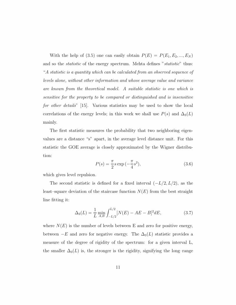
With the help of (3.5) one can easily obtain P (E) = P (E1, E2, ..., EN)

and so the statistic of the energy spectrum. Mehta defines ”statistic” thus:

“A statistic is a quantity which can be calculated from an observed sequence of

levels alone, without other information and whose average value and variance

are known from the theoretical model. A suitable statistic is one which is

sensitive for the property to be compared or distinguished and is insensitive

for other details” [15]. Various statistics may be used to show the local

correlations of the energy levels; in this work we shall use P (s) and ∆3(L)

mainly.

The first statistic measures the probability that two neighboring eigen-

values are a distance “s” apart, in the average level distance unit. For this

statistic the GOE average is closely approximated by the Wigner distribu-

tion:

P (s) =π

2s exp (−π

4s2), (3.6)

which gives level repulsion.

The second statistic is defined for a fixed interval (−L/2, L/2), as the

least–square deviation of the staircase function N(E) from the best straight

line fitting it:

∆3(L) =1

LminA,B

∫ L/2

−L/2[N(E)−AE −B]2dE, (3.7)

where N(E) is the number of levels between E and zero for positive energy,

between −E and zero for negative energy. The ∆3(L) statistic provides a

measure of the degree of rigidity of the spectrum: for a given interval L,

the smaller ∆3(L) is, the stronger is the rigidity, signifying the long–range

11

correlations between levels. For this statistic in the GOE ensemble:

∆3(L) =

L15, L≪ 1

1π2 logL, L≫ 1

. (3.8)

For the GUE there are similar results [14].

If the mean level density for the GOE is calculated, we obtain:

ρ(E) =

1πσ2

√2Nσ2 −E, |E| < 2Nσ2

0, |E| < 2Nσ2

. (3.9)

Although this is an unrealistic result, it can be explained by remembering

that global and local behaviours are on different scales and GOE is a good

model for local properties.

3.2 Comparison of GOE predictions with experimental data

Neutron resonance spectroscopy on a heavy even–even nucleus typically

leads to the identification of about 150 to 170 s–wave resonances with Jπ =

12

+located 8–10 MeV above the ground state of the compound system, with

average spacings around 10 eV and average total widths around 1 eV. Proton

resonance spectroscopy yields somewhat shorter sequences of levels with fixed

spin and parity, with typically 60 to 80 members. For the statistical analysis,

it is essential that the sequences be pure (no admixture of levels with different

spin or parity) and complete (no missing levels) [17]. Only such sequences

were considered by Haq, Pandey and Bohigas [18]. Scaling each sequence to

the same average level spacing and lumping together all sequences one leads

to the ”Nuclear Data Ensemble” (NDE), which contains 1726 level spacings.

12

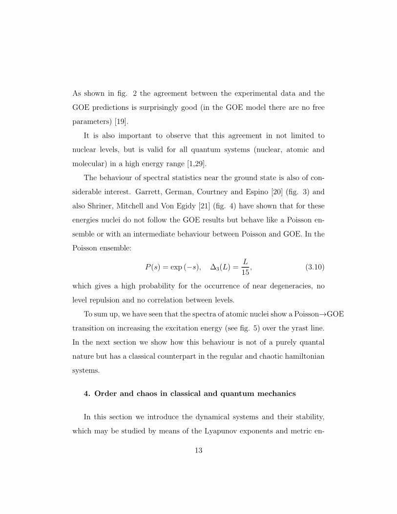
As shown in fig. 2 the agreement between the experimental data and the

GOE predictions is surprisingly good (in the GOE model there are no free

parameters) [19].

It is also important to observe that this agreement in not limited to

nuclear levels, but is valid for all quantum systems (nuclear, atomic and

molecular) in a high energy range [1,29].

The behaviour of spectral statistics near the ground state is also of con-

siderable interest. Garrett, German, Courtney and Espino [20] (fig. 3) and

also Shriner, Mitchell and Von Egidy [21] (fig. 4) have shown that for these

energies nuclei do not follow the GOE results but behave like a Poisson en-

semble or with an intermediate behaviour between Poisson and GOE. In the

Poisson ensemble:

P (s) = exp (−s), ∆3(L) =L

15, (3.10)

which gives a high probability for the occurrence of near degeneracies, no

level repulsion and no correlation between levels.

To sum up, we have seen that the spectra of atomic nuclei show a Poisson→GOE

transition on increasing the excitation energy (see fig. 5) over the yrast line.

In the next section we show how this behaviour is not of a purely quantal

nature but has a classical counterpart in the regular and chaotic hamiltonian

systems.

4. Order and chaos in classical and quantum mechanics

In this section we introduce the dynamical systems and their stability,

which may be studied by means of the Lyapunov exponents and metric en-

13

tropy. With the help of these quantities, we clarify the concept of ergodic

system giving a hierarchy of chaos. Then we extend the study to hamiltonian

systems, which are essential in order to study the transition order→chaos in

nuclear physics.

A dynamical system [22–25] is defined by N differential equations of the

first order:d

dt~z(t) = ~f(~z(t), t), (4.1)

where the variables ~z = (z1, ..., zN) are in the phase space Ω (the euclidean

space RN , unless otherwise specified). These equations describe the time

evolution of the variables and the system they represent.

A solution of the dynamical system is a vector function ~z(~z0, t), that

satisfies (4.1) and the initial condition:

~z(~z0, 0) = ~z0, (4.2)

often written simply ~z(t) without the initial condition dependence.

The time evolution of ~z ∈ Ω is obtained with the one parameter group of

diffeomorfism gt: Ω → Ω, so that:

d

dt(gt~z)|t=0 = ~f(~z, 0). (4.3)

The group gt is called phase flux and the solution is called orbit. The system

is called hamiltonian, if the dimension of Ω is even and there exists a function

H(~z, t) given by:

~f(~z(t), t) = J∇H(~z, t), (4.4)

where:

J =

0 I

−I 0

(4.5)

14

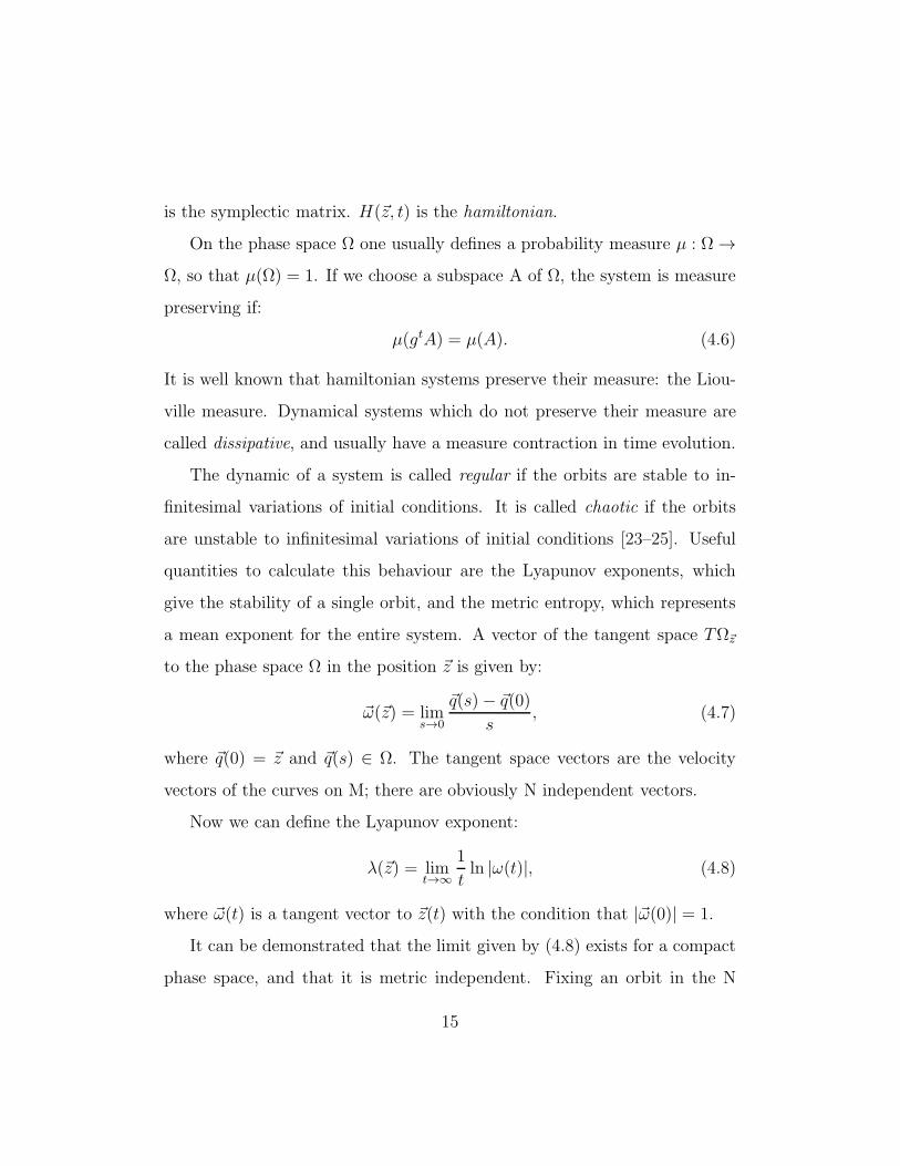
is the symplectic matrix. H(~z, t) is the hamiltonian.

On the phase space Ω one usually defines a probability measure µ : Ω →Ω, so that µ(Ω) = 1. If we choose a subspace A of Ω, the system is measure

preserving if:

µ(gtA) = µ(A). (4.6)

It is well known that hamiltonian systems preserve their measure: the Liou-

ville measure. Dynamical systems which do not preserve their measure are

called dissipative, and usually have a measure contraction in time evolution.

The dynamic of a system is called regular if the orbits are stable to in-

finitesimal variations of initial conditions. It is called chaotic if the orbits

are unstable to infinitesimal variations of initial conditions [23–25]. Useful

quantities to calculate this behaviour are the Lyapunov exponents, which

give the stability of a single orbit, and the metric entropy, which represents

a mean exponent for the entire system. A vector of the tangent space TΩ~z

to the phase space Ω in the position ~z is given by:

~ω(~z) = lims→0

~q(s)− ~q(0)

s, (4.7)

where ~q(0) = ~z and ~q(s) ∈ Ω. The tangent space vectors are the velocity

vectors of the curves on M; there are obviously N independent vectors.

Now we can define the Lyapunov exponent:

λ(~z) = limt→∞

1

tln |ω(t)|, (4.8)

where ~ω(t) is a tangent vector to ~z(t) with the condition that |~ω(0)| = 1.

It can be demonstrated that the limit given by (4.8) exists for a compact

phase space, and that it is metric independent. Fixing an orbit in the N

15

dimensional phase space, there are N distinct exponents λ1, ..., λN , called first

order Lyapunov exponents. If the orbit has positive Lyapunov exponents, it

is chaotic.

To characterize globally the chaoticity of a system, we introduce the met-

ric entropy. If α(0) is a partition of non–overlapping sets that completely

cover the phase space Ω at the initial instant:

α(0) = Ai(0) : Σ(E) = ∪iAi(0), Ai(0) ∩Aj(0) = φ, (4.9)

the partition α(0) can evolve in a discretized time flux:

α(0), α(1), α(2), ..., α(n). (4.10)

Then we define β(n) as the intersection set of all the sets at every instant:

β(n) = Bl(n) : Bl(n) = Ai(0) ∩ Aj(1) ∩ ... ∩ Ak(n). (4.11)

In this way, the number of sets defined by β(n) do not decrease when n is

increased. By introducing a probability measure µ preserved by dynamics,

one can define the metric information of the partition B(n):

In = −∑

i

µ(Bi(n)) lnµ(Bi(n)). (4.12)

The information In has the following properties:

(i) In = 0 if, and only if, there exists a set Bi(n) of the partition β(n) so

that µ(Bi(n)) = 1;

(ii) In assumes the maximum value when β(n) = B1(n), ..., BN(n) and

in this way µ(Bi(n)) =1N

∀i i.e. In = lnN .

16

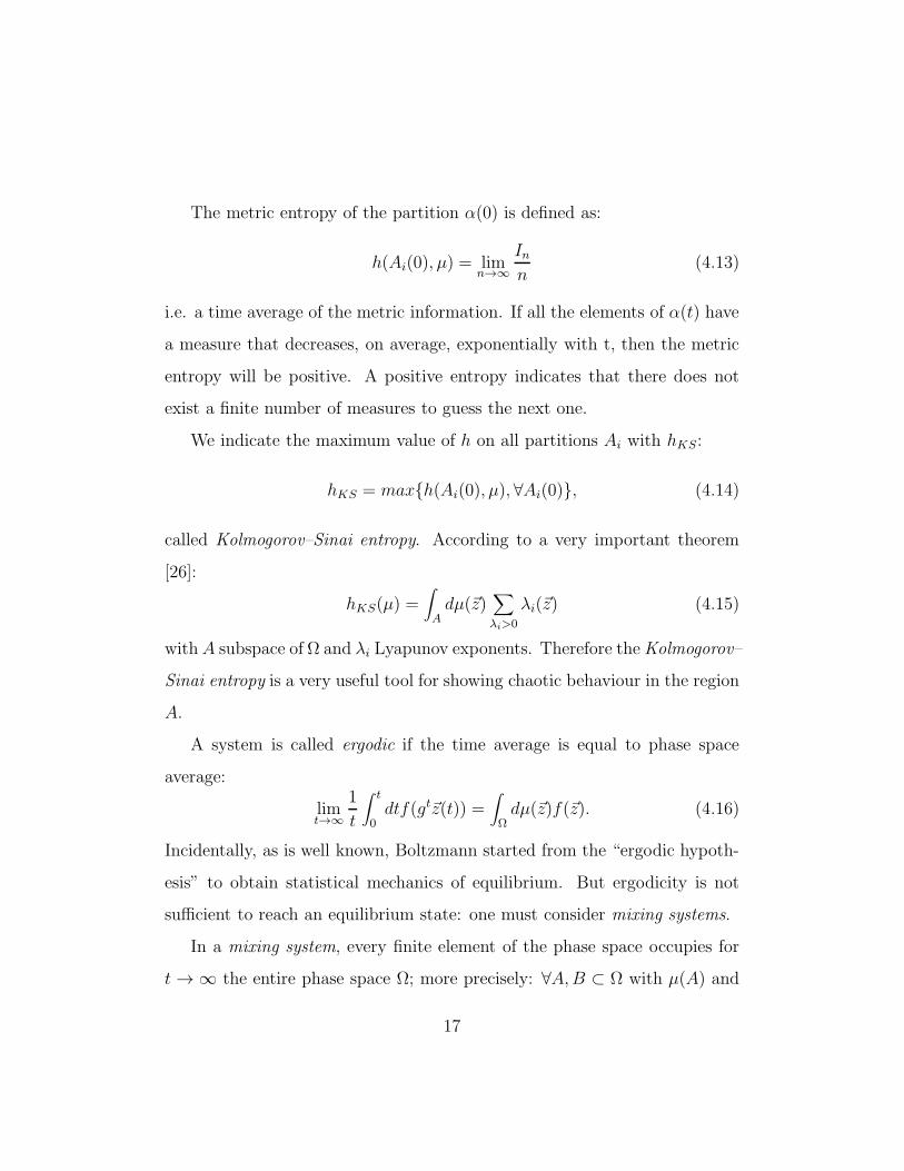
The metric entropy of the partition α(0) is defined as:

h(Ai(0), µ) = limn→∞

Inn

(4.13)

i.e. a time average of the metric information. If all the elements of α(t) have

a measure that decreases, on average, exponentially with t, then the metric

entropy will be positive. A positive entropy indicates that there does not

exist a finite number of measures to guess the next one.

We indicate the maximum value of h on all partitions Ai with hKS:

hKS = maxh(Ai(0), µ), ∀Ai(0), (4.14)

called Kolmogorov–Sinai entropy. According to a very important theorem

[26]:

hKS(µ) =∫

Adµ(~z)

∑

λi>0

λi(~z) (4.15)

withA subspace of Ω and λi Lyapunov exponents. Therefore theKolmogorov–

Sinai entropy is a very useful tool for showing chaotic behaviour in the region

A.

A system is called ergodic if the time average is equal to phase space

average:

limt→∞

1

t

∫ t

0dtf(gt~z(t)) =

∫

Ωdµ(~z)f(~z). (4.16)

Incidentally, as is well known, Boltzmann started from the “ergodic hypoth-

esis” to obtain statistical mechanics of equilibrium. But ergodicity is not

sufficient to reach an equilibrium state: one must consider mixing systems.

In a mixing system, every finite element of the phase space occupies for

t → ∞ the entire phase space Ω; more precisely: ∀A,B ⊂ Ω with µ(A) and

17

µ(B) 6= φ,

limt→∞

µ(B ∩ gtA)µ(B)

= µ(A). (4.17)

To have quantitative information of orbit separations, we must introduce

K–systems (Kolmogorov), which are mixing systems with a positive metric

entropy:

hKS > 0. (4.19)

Such systems are typical chaotic systems.

Among the K–systems, the most unpredictable ones are the B–systems

(Bernoulli), which have the Kolmogorov–Sinai entropy equal to the entropy

of every partition:

hKS = h(Ai(0), µ), ∀Ai(0). (4.20)

4.1 Classical chaos

In classical mechanics, the state of a system of coordinates qi and moments

pi, i = 1, ..., n in the N=2n dimensional phase space Ω, is specified by the

hamiltonian H = H(~p, ~q), with ~p = (p1, ..., pn), ~q = (q1, ..., qn) [22].

As is well known, the time evolution is obtained by the Hamilton equa-

tions:

qi =∂H

∂pi, pi = −∂H

∂qi. (4.21)

These equations, with the position ~z = (q1, ..., qn, p1, ..., pn), can be written

in the more compact form (4.4).

The hamiltonian system is integrable if there are n functions defined on

Ω:

Fi = Fi(~z) i = 1, ..., N (4.22)

18

in involution:

[Fi, Fj]PB =n∑

k=1

∂Fi∂qk

∂Fj∂pk

− ∂Fj∂qk

∂Fi∂pk

= 0, ∀i, j (4.23)

and linearly independent. [ , ]PB are the Poisson Brackets.

For the conservative systems we have F1 = H(~z) and also:

dFidt

= [H,Fi]PB = 0. (4.24)

Because there are n constants of motion, every orbit can explore only the n

dimensional manifold Ωf :

Ωf = ~z : Fi(~z) = fi, i = 1, ..., N (4.25)

If Ωf is compact and connected, it is equivalent to a n dimensional torus:

T n = (θ1, ..., θn) mod 2π (4.26)

There are n irreducible and independent circuits γi on Ωf and there exists a

canonical transformation:

(~p, ~q) → (~I, ~θ) (4.26)

generated by the function S(~q, ~I), so that:

Ii =∮

γid~q · ~p, θi =

∂S

∂Ii. (4.27)

The Ii are called action variables and the θi are called angle variables.

The moments ~p and coordinates ~q are periodic functions of ~θ with period 2π:

~q =∑

~m

~q~m(~I)ei~m·~θ, ~p =

∑

~m

~p~m(~I)ei~m·~θ (4.28)

19

where ~m = (m1, ..., mn) is an integer vector.

The hamiltonian depends only on action variables: H = H(~I), and so the

new equation of motion are:

θi =∂H(~I)

∂Ii= ωi(~I), Ii = −∂H(~I)

∂θi= 0, (4.29)

so:

θi = ωi(~I)t+ αi, (4.30)

where αi are constants and ωi are the frequencies on the torus.

The orbits of an integrable system are quasi–periodic, with n quasi–

periods:

Ti =2π

ωi, (4.31)

and the orbit is closed if there exists a period τ so that:

~θ(τ) = ~θ(0) + 2π ~D, (4.32)

with ~D integer vector. To have the closure, we must have:

~ω · ~mi = 0, (4.33)

and the period is:

τ =2π

ωc=

2πDi

ωi=Di

Ti. (4.34)

If we do not have n independent relations among frequencies, the orbits do

non close: we have the so called ”torus ergodicity”, but the motion is still

regular (see fig. 6).

Adding a small perturbation V (~I, ~θ) to an integrable hamiltonian H0(~I),

the total hamiltonian can be written:

H(~I, ~θ) = H0(~I) + χV (~I, ~θ), (4.35)

20

and, generically, the integrability is destroyed. As a consequence, parts of

phase space become filled with chaotic orbits, while in other parts the toroidal

surfaces of the integrable system are deformed but not destroyed; thus we

have a quasi–integrable system.

With growing χ, chaotic motion develops near the regions of phase space

where all the ωi are commensurate; or, more precisely, where the equation

(4.33) is obeyed by integer vectors.

Conversely, tori of the integrable system on which the ωi are incommen-

surate are deformed, but not destroyed immediately (KAM theorem). As χ

increases, the phase space generically develops a highly complex structure,

with islands of regular motion (filled with quasi–periodic orbits) interspersed

in regions of chaotic motion, but containing in turn more regions of chaos. As

χ grows further, the fraction of phase space filled with chaotic orbits grows

until it reaches unity as the last KAM surface is destroyed. Then the motion

is completely chaotic everywhere, except possibly for isolated periodic orbits

[22,23].

It is very useful to plot a 2n−1 surface of section P ⊂ Ω, called Poincare

section (see fig. 7). As shown in figure 8, for an integrable system with

two degrees of freedom, the x = 0 Poincare section of a rational (resonant)

torus is a finite number of points along a closed curve, while the section of

an irrational (non resonant) torus is a continuous closed curve.

Adding a perturbation, the section presents closed curves (KAM tori),

whose points are stable (elliptic), and also curves formed by substructures,

residua of resonant tori, whose points are unstable (hyperbolic). As the

perturbation parameter increases, the closed curves are distorted and reduced

21

in number.

4.2 Quantum chaos

In non relativistic quantum mechanics, the time evolution of a state |ψ >of a system with hamiltonian H is given by the Schrodinger equation [27]:

ih∂

∂t|ψ >= H|ψ > . (4.36)

The unitary time–evolution operator U(t) is:

U(t) = exp (−iHh), (4.37)

so that |ψ(t) >= U(t)|ψ >. If we choose a new state |ψ′

> near to |ψ > we

have:

< ψ′

(t)|ψ(t) >=< ψ′|U+(t)U(t)|ψ(t) >=< ψ

′ |ψ > . (4.38)

The distance between two quantum states is always time-independent, so

there is no chaos in quantum mechanics in the sense of time exponential

divergence of near states. However an interesting question is: whether there

are quantum–mechanical manifestations of classical chaotic motion. We shall

use the term quantum chaotic system in the precise, and restricted, sense of

a quantum system whose classical analogue is chaotic [24,25].

The studies of the eigenvalues of billiards with different shapes [28,29]

have shown that if the system is classically integrable the spectral statistics

are well modelled by the Poisson ensemble (3.10) and if the system is clas-

sically chaotic, by the GOE (3.6, 3.8) or GUE ensembles, depending on the

time–reversal symmetry (fig. 9).

22

When the classical dynamics of a physical system is regular, the short–

range properties of the corresponding quantal spectrum tend to resemble

those of a spectrum of randomly distributed numbers (the Poisson spec-

trum). This is because regular classical motion is associated with integrabil-

ity or separability of the classical equations of motion. In quantum mechanics

the separability corresponds to a number of independent conserved quanti-

ties (such as angular momentum), and each energy level can be characterised

by the associated quantum numbers. Superimposing the terms arising from

the various quantum numbers, a spectrum is generated like that of random

numbers, at least over short intervals. When the classical dynamics of a phys-

ical system is chaotic, the system cannot be integrable and there must be

fewer constants of motion than degrees of freedom. Quantum mechanically

this means that once all good quantum numbers due to obvious symmetries

etc. are accounted for, the energy levels cannot simply be labelled by quan-

tum numbers associated with certain constants of motion. The short–range

properties of the energy spectrum then tend to resemble those of eigenvalue

spectra of matrices with randomly chosen elements.

Berry and Tabor [30] predict level clustering for any integrable system

(with the exception of the harmonic oscillator that has equal spaced levels

[31]) in the asymptotic high energy regime, using the semiclassical (h → 0)

Einstein–Brillowin–Keller (EKB) quantization of action variables [24]:

En1,...,nN= H(I1 = h(n1 + a1/4), ..., IN = h(nN + aN/4)), (4.39)

where al is the Maslov index for the Il action variable. In one dimension:

a = 0 for the rotator and a = 12for the oscillator.

23

In quasi-integrable and chaotic systems the EKB quantization is not ap-

plicable but we can calculate the level density ρ(E) using a semiclassical

formula obtained by Gutzwiller [32,33]:

ρ(E) = ρ(E) + ρosc(E), (4.40)

where:

ρ(E) =1

(2πh)N

∫

d~pd~qδ(E −H(~p, ~q)), (4.41)

ρosc(E) =∑

j

Tj2f(λj)

cos (Sj(E)

h− ajπ

2). (4.42)

The summation is over all the periodic orbits of the classical phase space, Tj

is the j-periodic orbit period, f is a function of the j–periodic orbits Lyapunov

exponent and Sj(E) =∮

j d~q · ~p.With the help of (4.42) Berry [34] has calculated the semiclassical be-

haviour of the spectral rigidity ∆3(L) for a chaotic time–reversal system:

∆3(L) =

L15, L≪ 1

1π2 logL, 1 ≪ L≪ Lmax

12π2 log eLmax + oscillations, L≫ Lmax

, (4.43)

where Lmax = hρTmin

with Tmin the period of the shortest periodic orbits of

the classical phase space. The long–range periodic orbits contribute to the

universal behaviour, but there is also a non universal behaviour not predicted

by GOE.

In the next section, we describe a schematic shell model to show how an

order to chaos transition may occur by studying the classical and quantum

properties of the model.

24

5. Order to chaos transition in a schematic shell model

To study the transition from regular to chaotic states in atomic nuclei,

an extension of the two level Lipkin–Meshkov–Glick (LMG) model was pro-

posed by Meredith, Koonin and Zirnbauer (MKZ) [35–37]. The two level

LMG model has only one degree of freedom, i.e. the particle number in the

upper level, and so its classical limit does not have chaotic behaviour. The

generalization proposed by MKZ has the SU(3) symmetry and two degrees

of freedom: its classical limit shows an order to chaos transition.

The SU(3) model consists of M identical particles, labelled by the index

n, each of which can be in three single–particle states having energy ǫi. The

hamiltonian is:

H =3

∑

i=1

ǫiGii +3

∑

ij=1

VijG2ij , (5.1)

with ǫ3 = ǫ1 = ǫ and ǫ2 = 0, where Vij is the strength of the two–body

interaction between states i and j:

Vij = Vji and Vii = 0, (5.2)

with:

Gij =M∑

n=1

a+nianj . (5.3)

The operator a+ni creates a particle n in state i, and ani annihilates a particle

n from state i; each term of Gij takes a particle, n, out of state j and into

state i, and each Gii counts the particles in state i.

Applying the usual fermion anti–commutation rules to the ani operators,

we get:

[Gij , Ghk]− = Gikδjh − Gjhδik, (5.4)

25

and the 9 operators Gij are generators for U(3). Taking into account the

number conservation,∑3i=1 Gii =M , this becomes SU(3).

5.1 Classical limit

The quantum 4–dimensional phase space of SU(3) is U(3)/U(2) ⊗ U(1),

where U(2)⊗U(1) is the maximal stability subgroup which leaves the ground

state |00 > invariant up to a phase factor [38].

The coherent states of U(3)/U(2)⊗ U(1) are:

|SU(3), Φ >= Φ|00 >, (5.5)

where

Φ = exp 3

∑

i=2

(νiGi1 − ν∗i G1i), (5.6)

with νi complex numbers.

The Bergmann kernel is:

k(~z, ~z∗) =< SU(3), Φ|SU(3), Φ >= (1 + Z+Z)M , (5.7)

where Z is the 3x1 matrix:

Z = (zi) = (νi)tan(ν)

ν, (5.8)

with ν =√ν2ν

∗

2 + ν3ν∗

3 . The metric of U(3)/U(2)⊗ U(1) is then given by:

gij =∂2 ln k(~z, ~z∗)

∂zi∂z∗

i

, (5.9)

and the nondegenerate closed two–form ω of U(3)/U(2)⊗ U(1) is:

ω =3

∑

i,j=2

gijdzi ∧ dz∗j , (5.10)

26

with Poisson Brackets:

[f, g]PB = −i3

∑

i,j=2

gij[∂f

∂zi

∂g

∂z∗j− ∂f

∂z∗j

∂g

∂zi]. (5.11)

By introducing the canonical coordinates:

1√2(qi + ipi) =

√Mνiνsin ν, (5.12)

one can show that (5.12) will be transformed into the following canonical

form:

[f, g]PB =3

∑

i,j=2

[∂f

∂qi

∂g

∂pj− ∂f

∂pj

∂g

∂qi]. (5.13)

The semiquantal dynamics of this many–body system with fixed nucleons

number M is determined by varying the effective action:

S =∫

[1

2(~p · d~q − ~q · d~p)−H(~p, ~q)dt]. (5.14)

The result of such a variation is the set of classical–like dynamical equations:

dqidt

=∂H(~p, ~q)

∂pi,

dpidt

= −∂H(~p, ~q)

∂qi(5.15)

with the Hamiltonian functions given by:

H(~p, ~q) =< SU(3), Φ|H|SU(3), Φ > . (5.16)

Equation (5.15) is in fact equivalent to the time–dependent Hartree–Fock

(TDHF) dynamical equations. It should be noted that (5.15) is not a classical

limit because there is at least first–order quantum correlation in H(~p, ~q).

The phase space representation of the generators Gij in the coherent–

states basis is:

< |G11| >=1

2(2M − p2 − q2), (5.17)

27

< |G1i| >=1

2(qi + ipi)

√

2M − p2 − q2,

< |Gij| >=1

2(qj + ipj)(qi − ipi),

< |Gji| >=< |Gij| >∗,

where | > represents |SU(3), Φ > and (q22 + q23 + p22 + p23) ≤ 2M .

The quantum correlations of the quadratic function of the generators can

be computed and the results are:

∆(G2ij) =< |G2

ij | > − < |Gij| >2= − 1

M< |Gij | >2 . (5.18)

In this way the mean value of the hamiltonian in the coherent states repre-

sentation is:

H(~p, ~q) =ǫ12[2− (p22 + p23 + q22 + q23)] +

ǫ22(p22 + q22) +

ǫ32(p23 + q23)+ (5.19)

+χ

4[1− 1

M][(p22 + p23)

2 − (q22 + q23)2 + (q22 − p22)(q

23 − p23) + 4(q2q3p2p3)].

It should be noted that the phase space has been scaled in (5.19) such that

q22 + q23 + p22 + p23 ≤ 2, with χ = MV/ǫ. The classical limit of the SU(3)

model can be realized by the limit M → ∞, and, in this limit, the quantum

correlation ∆(G2ij) goes to zero (see 5.18). So the classical hamiltonian is

(ǫ = 1):

Hcl = −1 +1

2q22(1− χ) +

1

2q23(2− χ) +

1

2p22(1 + χ) +

1

2p23(2 + χ)+

+1

4χ[(q22 + q23)

2 − (p22 + p23)2 − (q22 − p22)(q

23 − p23)− 4q2q3p2p3], (5.20)

with the phase space given by Ω = (q2, q3, p2, p3) ∈ R4 : (q22 + q23 + p22 +

p23) ≤ 2. This hamiltonian represents two oscillators coupled non–linearly

28

by the parameter χ (the interaction between the nucleons). The system is

integrable if the interactions are neglected but the interactions break this

regular behaviour and produce an order to chaos transition.

5.2 Classical calculations

Using the Hamilton equations of (5.20), in order to analyze the stability

of the system, we calculated the periodic orbits of this model:

~z = J∇Hcl(~z, χ), (5.21)

where ~z = (q2, q3, p2, p3) , ∇ = ( ∂∂q2, ∂∂q3, ∂∂p2, ∂∂p3

), e J is the 4x4 symplectic

matrix:

J =

0 I

−I 0

, (5.22)

where I is the 2x2 identity matrix.

To explore the phase space Ω, we chose a 4–dimensional lattice of initial

conditions ~z0 = ~z(t = 0), ~z0 ∈ Ω. The side of the lattice has about 104 initial

conditions.

The time evolution of (5.21), with the initial condition ~z0, is obtained

using a 4th order Runge–Kutta method [39]. The following function can then

be constructed:

d(~z0, t) = d(~z0, ~zt) = |~zt − ~z0|, (5.23)

where ~zt = ~z(t). (5.23) is the function to minimize, with minimum value

equal to 0. To obtain a periodic orbit, it is not actually necessary to vary all

five parameters (~z0, t); in fact we can fix E = H(~z0) or t, which correspond

to focusing either on constant energy or constant period in the E–T plot.

29

Another algorithm [40] has been used to find the minimum of d. Since d

is the result of a complicated calculation and its derivatives are not available,

this algorithm is particularly useful in our case because the derivatives of d

are not required [41].

These periodic trajectories occur in one parameter families, each of which

describes a continuous curve in the energy–period plane (fig. 10); just as

in quantum mechanics the set of energy levels is characteristic of a given

hamiltonian H , so Hcl can be characterized by the plots E–T, where E is the

energy of a periodic trajectory and T the corresponding period.

If ~w is a vector of the tangent space TΩ~z of the phase space manifold Ω

at ~z, its time evolution is given by:

~w = J∂2H(~z)

∂~z2~w. (5.24)

By (5.21) and (5.24) the Lyapunov exponents can be calculated:

λ(~z) = limt→∞

1

tln |~w(t)|. (5.25)

In terms of the stability matrix M(0, t) [42], defined as:

Mij(0, t) =∂zi(t)

∂zj(0), (5.26)

λ(~z) can be written:

λ(~z) = limt→∞

1

tln |M(0, t)|, (5.27)

where |M(0, t)| is a norm of the matrix M(0, t).

This matrix can be calculated by solving its equations of motion:

M = J∂2H(~z)

∂~z2M, (5.28a)

30

with the initial conditions:

M(0) = I (5.28b)

where I is the 4x4 identity matrix. The calculation of the Lyapunov expo-

nents is related to that of the eigenvalues σi of the matrix M(0, T ):

λi(~z) =1

Tln σi. (5.29)

Now, using the unitariety of M, a periodic orbit is unstable if

Tr(M) > 4 or Tr(M) < 0 (5.30a)

and stable if

0 < Tr(M) < 4. (5.31b)

It is interesting to study the change of stability of periodic trajectories as

a function of χ. In figure 11 the ratio between the number of stable orbits

and the number of total orbits with period T < 30 is plotted vs χ. As can be

seen the sensitivity of the orbits to a small change of χ is quite different for

different values of χ, reflecting the transition order → chaos as the coupling

constant increases.

As mentioned in section 4.2, the calculation of the long–range behaviour

(non–universal) of ∆3 requires the knowledge of the shortest period Tmin of

the closed trajectories. For a chaotic system with time–reversal symmetry

[34]:

∆∞

3 =1

π2ln (eLmax)−

1

8, (5.32a)

where:

Lmax =hρ

Tmin(5.32b)

31

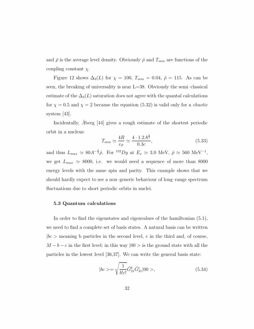
and ρ is the average level density. Obviously ρ and Tmin are functions of the

coupling constant χ.

Figure 12 shows ∆3(L) for χ = 100, Tmin = 0.04, ρ = 115. As can be

seen, the breaking of universality is near L=38. Obviously the semi–classical

estimate of the ∆3(L) saturation does not agree with the quantal calculations

for χ = 0.5 and χ = 2 because the equation (5.32) is valid only for a chaotic

system [43].

Incidentally, Aberg [44] gives a rough estimate of the shortest periodic

orbit in a nucleus:

Tmin ≃ 4R

vF≃ 4 · 1.2A 1

3

0.3c, (5.33)

and thus Lmax ≃ 80A−1

3 ρ. For 152Dy at Ex ≃ 3.0 MeV, ρ ≃ 560 MeV−1,

we get Lmax ≃ 8000, i.e. we would need a sequence of more than 8000

energy levels with the same spin and parity. This example shows that we

should hardly expect to see a non–generic behaviour of long–range spectrum

fluctuations due to short periodic orbits in nuclei.

5.3 Quantum calculations

In order to find the eigenstates and eigenvalues of the hamiltonian (5.1),

we need to find a complete set of basis states. A natural basis can be written

|bc > meaning b particles in the second level, c in the third and, of course,

M − b− c in the first level; in this way |00 > is the ground state with all the

particles in the lowest level [36,37]. We can write the general basis state:

|bc >=√

1

b!c!Gb

21Gc31|00 >, (5.34)

32

with√

1b!c!

the normalizing constant.

From the commutation relation (5.4) we can calculate the expectation

values of HM

and thus, eigenvalues and eigenstates of HM; in this way the

energy spectrum range is independent of the number of the particles:

< b′

c′| HM

|bc >= 1

M(−M + b+ 2c)δbb′δcc′ −

χ

2M2Qb′c′ ,bc, (5.35)

where:

Qb′c′,bc =

√

b(b− 1)(M − b− c+ 1)(M − b− c+ 2)δb−2,b′δcc′ (5.36)

+√

(b+ 1)(b+ 2)(M − b− c)(M − b− c− 1)δb+2,b′δcc′

+√

c(c− 1)(M − b− c+ 1)(M − b− c+ 2)δb,b′δc−2,c′

+√

(c+ 1)(c+ 2)(M − b− c)(M − b− c− 1)δb,b′δc+2,c′

+√

(b+ 1)(b+ 2)c(c− 1)δb+2,b′δc−2,c′

+√

b(b− 1)(c+ 1)(c+ 2)δb−2,b′δc+2,c′

and χ = MV/ǫ. The expectation value < HM> is real and symmetric. For

any given number of particles M, we can set up the complete basis state,

write down the matrix elements of < HM

> and then diagonalize < HM

>

to find its eigenvalues. < HM

> connects only states with ∆b = −2, 0, 2

and ∆c = −2, 0, 2 which makes the problem easier. We group states with

b,c even; b,c odd; b even and c odd; b odd and c even. This means that

< HM> becomes block diagonal containing 4 blocks which can be diagonalized

separately; these matrices are referred to as ee, oo, oe and eo.

To separate regular and chaotic state in a quantum system a powerful

tool is the study of spectral statistics. We obtain [45] a good agreement with

33

GOE in the classically chaotic region and, in the classically regular region,

a good agreement with Poisson statistic (see fig. 13). In this figure the

continuous curve is the Brody distribution, discussed in section 6.5.

On the basis of the semiclassical torus quantization, the presence of cross-

ings in a small χ neighbourhood may be interpreted as the signature of quasi

crossing in the true system, and thus as a signature of torus destruction,

when the exact levels are “split” at the crossing [46–48].

Another method to study the quantum stochasticity is the sensibility of

the energy levels to variations of the perturbation parameter; the behaviour

of the curvature of the energy level E(χ) in a small χ neighbourhood is an

example [49].

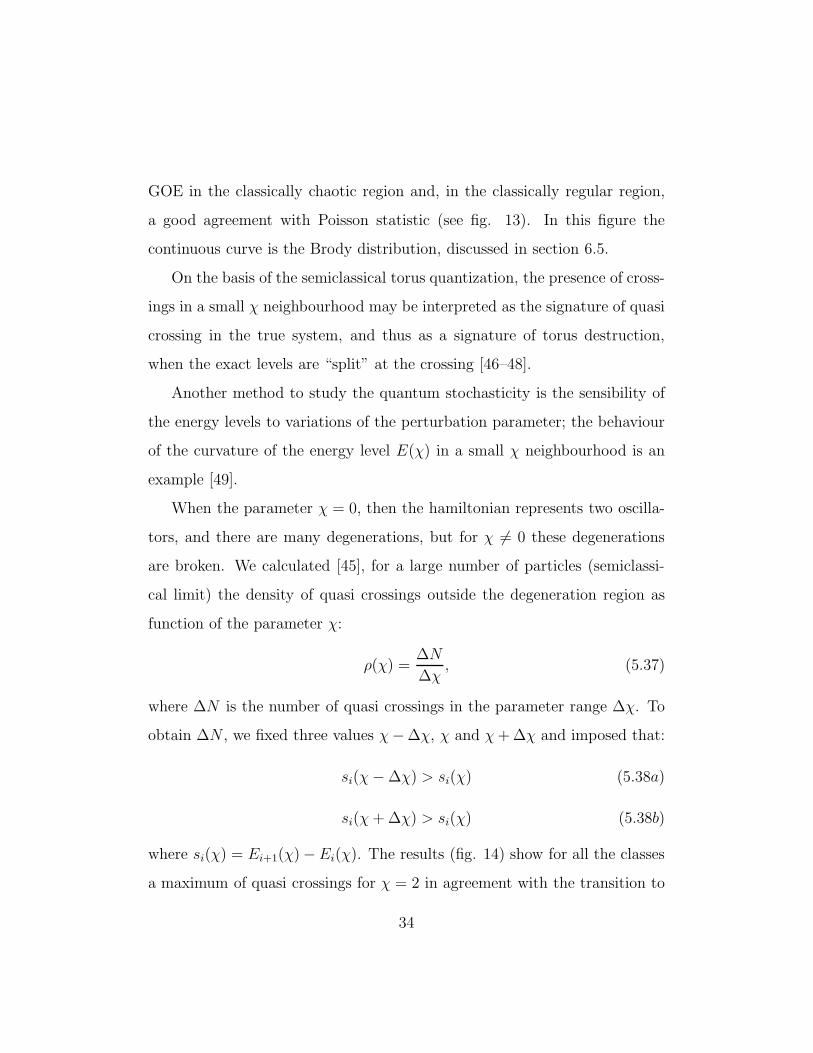
When the parameter χ = 0, then the hamiltonian represents two oscilla-

tors, and there are many degenerations, but for χ 6= 0 these degenerations

are broken. We calculated [45], for a large number of particles (semiclassi-

cal limit) the density of quasi crossings outside the degeneration region as

function of the parameter χ:

ρ(χ) =∆N

∆χ, (5.37)

where ∆N is the number of quasi crossings in the parameter range ∆χ. To

obtain ∆N , we fixed three values χ−∆χ, χ and χ+∆χ and imposed that:

si(χ−∆χ) > si(χ) (5.38a)

si(χ+∆χ) > si(χ) (5.38b)

where si(χ) = Ei+1(χ)−Ei(χ). The results (fig. 14) show for all the classes

a maximum of quasi crossings for χ = 2 in agreement with the transition to

34

chaos of fig. 12.

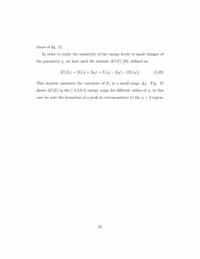
In order to study the sensitivity of the energy levels to small changes of

the parameter χ, we have used the statistic ∆2(E) [50], defined as:

∆2(Ei) = |Ei(χ+∆χ) + Ei(χ−∆χ)− 2Ei(χ)|. (5.39)

This statistic measures the curvature of Ei in a small range ∆χ. Fig. 15

shows ∆2(E) in the [–0.5,0.5] energy range for different values of χ; in this

case we note the formation of a peak in correspondence to the χ = 2 region.

35

6. Wave function behaviour and EM decay of regular and

chaotic states

As we have seen in the previous sections, it is now well known that in

atomic nuclei there are two different states: regular and chaotic. These

states can be highlighted with the aid of various statistics. The statistics

we have considered before concern the eigenvalues of the system, and the

most frequently used are those of level spacing; i.e. the nearest neighbour

distribution, P (s), and the stiffness of the spectrum ∆3(L). Since these

statistics display clearly different behaviour depending on the regularity or

chaoticity of the nucleus, they are very useful to distinguish between the two

regimes and, at the same time, characterize the transition from one region

to the other.

However, it is well known that, in general, the wave functions and the

transition probabilities are much more sensitive to the purity of states than

the eigenvalues are. Consequently, it is interesting to undertake the study of

statistics directly related to the wave functions with the aim of characterizing

the ordered or chaotic behaviour of atomic nuclei.

Using the SU(3) schematic shell model for the nucleus, described in Sec-

tion 5, we have studied the various statistics concerning the wave functions,

such as the intensity of the momenta of the wave function Im, the information

measure or entropy S, and the correlation functions Kn,m.

The momenta Im and the information measure S are defined [51]:

Im =∑

b,c

|ψ(b, c)|2m, (6.1)

36

S = −∑

b,c

|ψ(b, c)|2 ln |ψ(b, c)|2. (6.2)

Figure 16 shows that the lower momenta (m=2,3,4) diverge in the regular

region but have a constant behaviour in the chaotic region, as predicted by

[52].

The information measure S also shows different behaviours in the two

regions, assuming high values in the chaotic region and low values in the

regular region because wave functions are localized (see fig. 17).

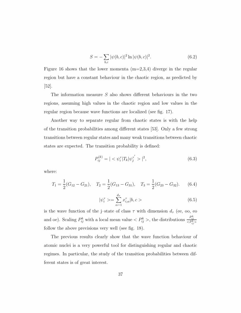
Another way to separate regular from chaotic states is with the help

of the transition probabilities among different states [53]. Only a few strong

transitions between regular states and many weak transitions between chaotic

states are expected. The transition probability is defined:

P(k)ij = | < ψτi |Tk|ψτ

′

j > |2, (6.3)

where:

T1 =1

2(G12 −G21), T2 =

1

2(G13 −G31), T3 =

1

2(G23 −G32). (6.4)

|ψτi >=dτ∑

α=1

xτi,α|b, c > (6.5)

is the wave function of the j–state of class τ with dimension dτ (ee, oo, eo

and oe). Scaling P kij with a local mean value < P k

ij >, the distributionsP kij

<P kij>

follow the above previsions very well (see fig. 18).

The previous results clearly show that the wave function behaviour of

atomic nuclei is a very powerful tool for distinguishing regular and chaotic

regimes. In particular, the study of the transition probabilities between dif-

ferent states is of great interest.

37

6.1 Decay of regular and chaotic states

Recently, new interest has been shown in the study of the decay of unsta-

ble quantum states. In this section we briefly review the literature of major

interest. The section is organized as follows: first, we look at the current

experimental stage to illustrate the reasons and interest for studying the de-

cay of quantum systems. Secondly, we review the main current theoretical

approaches to the problem. We begin with the study of ”warm” rotational

nuclei, to continue with that of unstable systems described by means of an

anti-hermitian effective hamiltonian. Finally, we briefly discuss the Interact-

ing Boson Model (IBM) that affords a wide spectrum of applications, from

vibrational to rotational nuclei as well as transitional regions.

6.2 Experimental stage

The new generation of experimental instruments like GASP, EUROBALL,

EUROGAM, etc [54], which provide a resolution in the order of a hundred

times greater than that of the previous generation, will open a new way in

nuclear spectroscopy research. Over the last few years, as discussed above,

great interest has been shown in the study of the properties of the atomic

nuclei from a statistical point of view. This has made it possible, with the

aid of the Random Matrix Theory [14], to distinguish between regular and

chaotic regimes, the onset of chaos, the transition from one regime to the

other, etc.

Let us now turn our attention to the recent statistical analysis of γ-ray

spectra of ”warm” rotational nuclei by Garrett, Hagemann and Herskind

38

[55]. In their work, two and three-fold energy correlation measurements

between gamma rays were analyzed to investigate high spin states of the so

called quasi-continuum that spreads up to 5-10 MeV above the yrast line.

This study had already been proposed by Guhr and Weidenmuller [56] who

stressed the coexistence of collectivity and chaos in nuclei at several MeV of

excitation energy; they suggested the study of stretched collective E2 decays

of high spin states in deformed even-even nuclei at, or above, the yrast line.

It was shown that the collective E2 transitions from states of spin I, located

several MeV above the yrast line, populate many states (of the same parity)

of (I − 2) spin rather than a single one (as happens with the E2 transitions

from states near the yrast line, where a well defined rotational band structure

exists). Thus the transition strength is spread over an energy interval that

is called rotational damping width. The analysis of the group of Herskind is

indeed oriented in this direction. By performing a fluctuation analysis of the

2–D Eγ1xEγ2 spectrum they obtained information on the number of decay

routes the nuclear decay flow takes to go from the initial high spin state to

the damped region (which is supposed to be in the diagonal valley, x = y, of

the 2–D spectra). A schematic illustration of the average flow of γ-ray decay

from high-spin states induced by heavy-ion compound reactions is shown in

fig. 19.

The 2–D and 3–D fluctuation analysis method developed by this group

[55] has been applied to the spectra from a triple coincidence experiment

made by the Manchester–Daresbury–Copenhagen–Bonn collaboration at the

Daresbury Tandem Accelerator. The reaction consisted in bombarding 124Sn

by a beam of 48Ca of 215 MeV, to form the residual nuclei of 168Y b at the

39

highest spin Imax = 60h. From the fluctuation analysis done on 168Y b they

concluded that the rotational correlations originating from well defined ro-

tational band structures only exist up to 1 MeV above the yrast line. Over

this limit the main decay routes spread out into many branches. This may

be accounted for by the rotational damping phenomenon, as Guhr and Wei-

denmuller [56] had previously suggested in 1989 from a theoretical calcula-

tion with a GOE hamiltonian weakly perturbed by a residual interaction. In

the conclusions of this work, the authors proposed the measurement of the

spreading width of E2–strength for a high–spin state well above the yrast

line, to determine the possible onset of chaos in ”warm” deformed nuclei.

The fluctuation analysis mentioned above has in fact taken up this sugges-

tion.

The first conclusions extracted from this new analysis of γ-ray data sug-

gest that there is much interest to be had from the study of states near

and above the yrast line, ”warm” rotational nuclei and the decay of unsta-

ble quantum states. New theoretical attention has been devoted to these

phenomena.

6.3 Rotational damping motion

Due to the recent experiments in γ-ray detection, a renewed interest has

developed in the the study of the decay of chaotic states and the possibility of

clarifying the mechanisms by which an excited nucleus (6–8 MeV over yrast

line) undergoes a transition from a regular to a chaotic behaviour.

In this sense, the work of Matsuo, Dossing, Herskind and Frauendorf [57]

40

is very interesting. They investigate the properties of energy levels and rota-

tional transitions as a function of the excitation energy, in ”warm” deformed

nuclei, and show that, at an excitation energy of the order of Ex ≃ 8 MeV,

there is considerable fragmentation of the rotational E2 strength distribution

when it is represented against the γ energy (see fig. 20). This fragmentation

with increasing energy is due to the mixing of the rotational bands caused

by the Surface Delta Interaction (SDI):

V (1, 2) = 4πV0δ(r1 −R0)δ(r2 − R0) ·∑

λ,µ

Y ∗

λ,µ(r1) · Yλ,µ(r2), (6.6)

which contains all the possible multipolarities. Actually, the high multipole

components of this SDI are shown to be responsible for the mixing of rota-

tional bands which is reflected in fluctuations typical of chaotic behaviour.

The strength fluctuations of the E2 transitions, for instance, obey a Porter–

Thomas distribution above a certain excitation energy, assumed to be the

threshold for the realization of quantum chaos in the system (fig. 21).

In particular, the same authors have also studied high spin levels in nuclei

with a cranked shell model extended to include residual two-body interactions

[58]. Here again the residual interaction induces the transition from a regular

to a chaotic regime, since when the rotational bands do not interact, γ-ray

energies behave like random variables, i.e., they obey a Poisson distribution

typical of a regular regime. On the contrary, when the residual interaction is

added, at an excitation energy over 600 KeV, a gradual rotational damping

is established, and, at 1.8 MeV above the yrast line, the complete damping

is observed and typical GOE fluctuations of the energy levels and transition

strengths are produced (fig. 22).

41

A similar approach is used by Aberg [59] to study the rotational damping

of rapidly rotating nuclei. As in the preceeding approach, a cranked Nilsson

model with a schematic residual interaction is used to study the distribution

of the E2-strength, and γ−γ correlations. In particular the normal deformed

(ND) 168Y b and the superdeformed (SD) 152Dy are studied, and the different

behaviours of these nuclei with increasing energy are compared. The main

difference between the approach of Aberg and that of the authors of ref.

[58] is that in the former the energies of the np-nh states are given in the

laboratory frame as functions of the angular momentum I. So, diagonalization

is performed for each fixed I value. This is reflected in a change of the

individual energies, but the conclusions regarding the different statistical

properties are the same. The Aberg approach is perhaps more useful if a

direct comparison with Eγ−Eγ experimental spectra is to be carried out. The

”classical” eigenvalue statistics are studied (i.e. P (s), ∆3(L)) with special

regard to the ∆3(L) since it gives a measure of long-range correlations. In this

model the transition from order to chaos is brought about by changing the

strength of the two-body force (∆) which is taken as a parameter, V2 = ±∆,

where the sign is chosen randomly to avoid coherent effects. Following the

procedure of Brody [60], the ∆3(L) spectrum is fitted with a single parameter,

q, to study the mixing between the Poisson and GOE distribution:

∆3(L, q) = ∆P3 [(1− q)L] + ∆GOE

3 (qL). (6.7)

The dynamical properties are studied in this model and again a rotational

damping is manifested in the fragmentation of E2 strength in many daughter

states. The average standard deviation of the E2-strength function saturates

42

for sufficiently large values of the strength of the two-body residual interac-

tion, following the same trend as q parameter, which gives the mixing of a

Poisson and GOE behaviour of spectrum properties (see figs. 23–24).

In addition to the previously mentioned rotational damping, Aberg also

studies motional narrowing, i.e., the decrease of the width of nuclear mag-

netic resonances when the temperature increases, a phenomenon which may

be studied in a simple two-band model. The narrowing of the strength func-

tion is accomplished by a change from a Gaussian shaped strength to a

Breit-Wigner shape. This phenomenon is understood in terms of time scales:

when the time scale of the fluctuations in available rotational frequencies is

much less than the time the wave function takes to spread out over the basis

states, the intensity spectrum is Gaussian, while in the opposite case the

corresponding spectrum is of the Breit-Wigner type.

Since, due to the motional narrowing the E2 strength may become very

narrow at the end, a small number of relatively strong E2 transitions may be

observed, and, consequently, a ”suppression of chaos”. In fact the transition

entropy defined as [44]:

HT,α = −∑

α′

[Mαα′ ]2 · ln([Mαα′ ]2), (6.8)

where:

Mαα′(I) =< α′, I − 2|M(E2)|α, I > (6.9)

decreases when motional narrowing sets in.

The γ − γ correlations between consecutive γ-rays are also analyzed to

study the fragmentation of E2 strength. Correlations are revealed at small

43

excitation energies or when a small ∆ is used, while at high excitation energies

these correlations disappear.

6.4 The study of unstable systems using a complex effective

hamiltonian

A different and more general approach to the study of unstable quan-

tum systems is that of Sokolov and Zelevinsky [61] and more recently that

of Mizutori and Zelevinsky [62], in which the statistical theory of spectra,

formulated in terms of random matrix theory, is generalized to treat unsta-

ble states, i.e. those coupled to open channels. In this way the influence of

the coupling with the continuum on the properties of internal states can be

better understood.

In general, as we have seen up to now, the level statistics are treated as if

the states were stationary but, in reality, all excited states are resonances em-

bedded in the continuum. So if one intends to study the most general states

of a system (including the unstable ones) a new approach to the problem has

to be used.

When the widths of the states are small as compared with level spac-

ings, the approximation of discrete levels is reasonable for long-lived states.

However, when the widths increase and the levels overlap, the effects of the

finite lifetime of those become crucial and the application of a random matrix

ensemble of hermitian hamiltonians is not enough appropriate.

Since the standard gaussian ensembles are applicable to discrete station-

ary states, while an excited state decays via open channels, the use of a

44

non-hermitian effective hamiltonian H is imposed to take into account the

width of the states due to their finite life [61,62].

Within this model the reaction amplitudes are represented, using the

general theory of resonant nuclear reactions, as sums of pole terms in the

complex plane. Such poles, ǫn = En − (1/2)iΓn are the eigenvalues of the

non-hermitian effective hamiltonian H = H− (i/2)W where H is the hermi-

tian part belonging to the GOE. The amplitudes of the antihermitian part,

W , have a separable structure Wnm = ΣcAcnA

cm due to the unitarity of the

scattering matrix, where Acn are the amplitudes for the decay of intrinsic

states of the system, |n > (n=1,...N) into different channels, c (c=1,....k)

and that must be real according to time reversal invariance of the full hamil-

tonian, H. Those eigenvalues correspond to the intermediate unstable states

of energies En and widths Γn.

Decaying systems are hence described by ensembles of random non-hermitian

hamiltonians represented by N-dimensional matrices where the hermitian

part of the effective hamiltonian, H, belongs to the GOE. The decay ampli-

tudes Acn, on the other hand, are assumed to be Gaussian random variables

completely uncorrelated with the matrix elements of H and among each

other.

Within this model the distribution function of complex energies, the level

spacing distribution and the width distribution are studied in ref. [61,62] for

weak and strong coupling to the continuum, as well as for the transitional

region.

The authors of ref. [62] discussed in great detail the single channel case:

45

k = 1. They assumed that < An >= 0, < Hmn >= 0, and:

< Hnn′Hmm′ >=a2

4N(δmn′δm′n + δmnδm′n′ ). (6.10)

The strength of coupling to the continuum is given by the overlap parameter

χ = η/a = 2 < Γ > /D where η =∑

j < Γj >; D is the mean level spacing.

When the overlap parameter is small (χ << 1), that is, when coupling

with the continuum is weak, the hermitian part H dominates, while the

antihermitian part, W , prevails in the opposite limit (χ >> 1).

Typical signatures of the transition from weak to strong coupling are ob-

served: first, concerning the level spacing distribution, which gives the sim-

plest characterization of spectral correlations, it is observed that for a weak

coupling (where the hermitian part, H , of the effective hamiltonian domi-

nates) the distribution of levels corresponds to a Wigner distribution, and

deviations from it are small. As the coupling with the continuum increases,

the Wigner function ceases to be a good approximation to the GOE and a

new feature is observed: the level repulsion at short distances disappears.

The authors of ref. [62] have fitted the P (s) distribution by a simple

one-parameter superposition of the normalized Wigner, PW , and Gaussian,

PG distributions, that is:

P (s) = αPW (s) + (1− α)PG(s) =1

∆[α

∆s+ (1− α)

√

2

π] exp (− s2

2∆2), (6.11)

where the parameter ∆ is determined, for a fixed α, by the mean level spacing:

D = ∆[

√

π

2α +

√

2

π(1− α)]. (6.12)

In the fig. 25 the trend of the mixing parameter α for the P (s) as a func-

tion of the coupling constant χ is plotted, showing a pronounced minimum

46

(α = 0.74) at the transition point χ = 1. Both small and large values of χ

correspond to the nearest level statistics close to a Wigner distribution PW .

It is well known that the GOE implies rigid spectra with small level spacing

fluctuations. So, we can conclude that coupling to the decay channels softens

the spacing distribution so that the spacing fluctuations increase gradually

in the transition region.

As regards the distribution of complex energies, it is has been observed

that, for a random matrix ensemble, the widths distribution corresponds to

a Porter-Thomas one, i.e.:

P PT (Γ) =1

√

2π < Γ > /Γ)exp (−< Γ >

2Γ). (6.13)

This, however, is no longer correct when the level spacings become very small

compared to the widths, i.e., when the overlap between neighbour states is

considerable. This is a consequence of the coupling to the continuum, since

for weak coupling the typical widths are small compared to spacings. When,

however, the coupling to the continuum is important, the widths become

larger than the mean level spacing. This behaviour had already been observed

for complex random matrix ensembles [63] and in chaotic dissipative systems

[64].

The most interesting statistic for highlighting the phase transition is the

width distribution. In fig. 26 the widths, plotted as a function of the coupling

parameter χ, show a collectivization. The mean fraction < Γ1/∑

j Γj > of

the total width is accumulated by the broadest state Γ1.

In conclusion, we can say that within these works a standard statistical

spectroscopy of discrete levels and unstable states, as well as for the transi-

47

tional region, has been performed using ensembles of random non-hermitian

hamiltonians represented by N-dimensional matrices. They show [61,62] that

the instability of states changes the statistics remarkably, removing level re-

pulsion when distances are smaller than widths. When the coupling to the

continuum increases, that is, when the matrix elements of the antihermitian

part of the effective hamiltonian become comparable with the spacings of

eigenvalues of the hermitian part, a transition to a new regime occurs.

Related to the study of unstable systems and in the same spirit as the

preceeding work, a paper by Haake et al. [65] is noteworthy. The authors

study the level density of different classes of random non-hermitian matrices,

H = H+ iΓ, where the damping, Γ, is chosen quadratic in Gaussian random

numbers, to describe the decay of resonances through various channels. When

the notion of level spacing is extended to the Euclidian distance between com-

plex eigenvalues of non-hermitian operators, two different behaviours of P (s)

statistic (as in the ordinary case of real eigenvalues with the Wigner and Pois-

son statistics) allow the distinction between regular and chaotic dynamics:

cubic repulsion tends to be typical under conditions of global classical chaos

while linear repulsion signals classical integrability. This classification also

arises for dissipative systems [66].

6.5 The IBM model in the study of unstable systems

The profound understanding of the statistics of low-lying levels of nuclei

and the underlying chaotic dynamics requires realistic theoretical models of

the nucleus. In general, the models used have only two degrees of freedom.

48

However, since the quadrupole deformation plays an important role in col-

lective nuclear dynamics, a realistic model requires at least five degrees of

freedom.

The work of Whelan and Alhassid [67] have been along these lines. Us-

ing the Interacting Boson Model (IBM) [3], whose classical limit is obtained

with coherent states and which provides a good description of low-lying en-

ergy levels and EM transitions of heavy nuclei, they studied, classically and

quantum mechanically, the chaotic properties of low–lying collective states of

atomic nuclei. The six degrees of freedom come from one monopole s-boson

(0+) and five dµ (µ = −2, ..., 2) bosons (2+) with which a U(6) dynamical

algebra is constructed. The most general hamiltonian is then constructed

with all one and two-body scalars that conserve the total number of bosons,

N = ss+ +∑

µ d+µ dµ.

The most useful parameterization of the IBM hamiltonian is given by:

H = E0 + c0nd + c2Qχ ·Qχ + c1L

2, (6.14)

where nd = d+ · d is the number of d-bosons, L is the angular momentum

and Qχ is the quadrupole operator:

Qχ = (d+ × s+ s+ × d)(2) + χ(d+ × d)(2), (6.15)

that depends on a parameter χ, and where dµ = (−)µdµ so that dµ transforms

under rotations like d+µ .

Its classical limit is obtained for the number of bosons going to infinity,

since 1/N plays the role of h. That classical limit is:

h = ǫ0 + c[ηnd − (1− η)qχ · qχ] + c1L2, (6.16)

49

where:η

1− η= − c0

Nc2, c =

c0η, (6.17)

with 0 < η < 1. In an algebraic model like this, a dynamical symmetry

occurs when the hamiltonian can be written as a function of the Casimir

invariants C of a chain of subalgebras of the original algebra. So, the authors

of ref. [67] analyze the rotational nuclei (SU(3) symmetry), vibrational nuclei

(U(5) symmetry) and γ-unstable nuclei (O(6) symmetry):

U(6)⊃U(5)⊃O(5)⊃O(3) (vibrational nuclei)

U(6)⊃SU(3)⊃O(3) (rotational nuclei)

U(6)⊃O(6)⊃O(5)⊃O(3) (γ-unstable nuclei).

The authors study the character of the classical dynamics of a nucleus

described by the classical limit of the quantum IBM hamiltonian. As a first

result, they found that the quantal fluctuations, which are well correlated

with the classical results, are independent of the number of bosons. The

transitions between the different dynamical symmetries of the model (i.e.,

between the different dynamics of nuclei) with the variation of the parameter

χ, of both classical and quantal hamiltonian, are studied.

The transition between deformed rotational nuclei (SU(3)) and spherical

vibrational nuclei (U(5)) is obtained for χ = −1/2√7 and 0 < η < 1. With

these parameters, classical and quantal measures of chaos are studied: the

average maximal Lyapunov exponent λ and the fraction of chaotic trajecto-

ries σ, on the one hand, and the parameter ω of the Brody distribution of

level spacing [60] on the other:

Pω(s) = Asω exp (−αsω+1). (6.18)

50

The Brody distribution, as the ∆q3(L) mentioned above, interpolates between

a Poisson distribution (ω = 0) for a regular system and a Wigner one (ω = 1)

for a chaotic system. α and A are chosen such that Pω(s) is normalized to 1

and < S >= 1. A second quantal measure of chaos is ν, which characterizes

the B(E2 : I → I) distribution for the levels with I = 2+:

Pν(y) =1

Γ(ν2)(

ν

2 < y >)ν2 y

ν2−1 exp (− νy

2 < y >), (6.19)

where:

y = | < f |T |i > |2, (6.20)

|i > and |f > being, respectively, the initial and final states and T the

transition operator. P (y)dy is the probability of having intensity P (y) in

the interval dy around y. P (y) reduces to a Porter-Thomas distribution for

ν = 1 (chaotic limit) and, as the system becomes more regular, ν decreases

towards small positive values.

The maximum of chaos is obtained for η = 0.5 − 0.7. The quantal re-

sults show a strong correlation with the classical dynamics, since ω and ν

are largest around η = 0.5 − 0.7. Secondly, the transition between rota-

tional nuclei (SU(3)) and γ-unstable nuclei (O(6)) is obtained for η = 0 and

−1/2√7 < χ < 0, chaos being settled for intermediate values of χ. Finally,

the transition between γ-unstable (O(6)) and vibrational nuclei (U(5)), for

χ = 0 and 0 < η < 1, is always completely regular.

The most important result is, on the one hand, the discovery of a new

nearly regular region that lies between a rotational (SU(3)) and vibrational

(U(5)) regime of the nucleus, and that is not related to any of the known

dynamical symmetries of the model. Since the fraction of chaotic trajectories

51

(σ) is < 0.3, that region is not completely regular. The signatures of this

nearly regular region are identified by the rather sharp minimum in all mea-

sures of chaos, as seen in fig. 27. The authors suggest that this new nearly

regular region may be connected with a previously unknown approximate

symmetry of the model. On the other hand, a spin dependence of the degree

of chaoticity is revealed. When both classical (λ,σ) and quantal (ω,ν,q) mea-

sures of chaos are plotted versus spin, an interesting dependence is found: in

all measures (except λ) a weak dependence on the spin, at low and medium

spins, is found. However, at high spins (I > 20h) there is a rapid decrease of

chaoticity and the motion becomes regular.

In conclusion, strong correlations are observed between the onset of clas-

sical and ”quantum” chaos. Although the IBM model can be useful for the

study of the degree of chaoticity of low-lying collective states of nuclei, at

higher spin and/or energy, bosons may break into quasi-particles and it is also

important to take into account the additional fermionic degrees of freedom,

to obtain a realistic description [4].

In this section we have presented some of the most interesting recent

works, which have attempted to explain the mechanisms of the decay of

quantum states and its connection with the onset of chaos.

The theoretical efforts are also supported by the new detector genera-

tion, which, with their higher resolution, can provide a new and profound

knowledge in the field of nuclear spectroscopy.

52

7. Conclusions and open problems

To conclude this presentation of some regular and chaotic aspects in nu-

clear dynamics, it is important to remember two points. The first is the good

agreement between the theoretical previsions concerning the Poisson→GOE

transition and the experimental data; the second is the possibility of studying

the order to chaos transition using simple models.

As pointed out by many authors (see for instance ref. [1]), the static

nuclear mean field is too regular (as witnessed by the existence of shell struc-

ture) to be responsible of chaotic behaviour, and chaos must be caused by

residual interaction, as shown in the models discussed above. Because of the

exclusion principle, the role of the latter increases with the excitation energy.

This makes one wonder whether nuclear motion might be more regular in the

ground–state region than, say, at neutron threshold. Indeed, at several MeV

excitation energy, collective states and giant resonances acquire substantial

spreading widths [1]. They lose their individuality as excitation states, and

show up only as bumps in strength functions. The same kind of statement

applies also to rotational bands 1 or 2 MeV above the yrast line. Much work

remains to be done to elucidate the role of chaotic motion and its interplay

with collectivity.

There is also the problem of showing which properties of the nucleon–

nucleon interaction justify the use of random matrix models. These, accord-

ing to ref. [1], are related to nonintegrability and chaos, but the matter

requires further research to obtain a deeper understanding of the problem.

We have shown that chaos in nuclei is a rich field; it permeates many

53

aspects of nuclear structure and reactions, and gives rise to new analyses of

the experimental data.

54

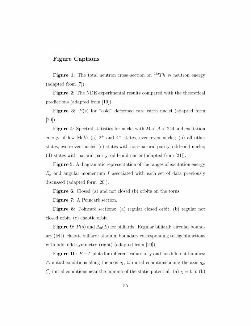
Figure Captions

Figure 1: The total neutron cross–section on 232Th vs neutron energy

(adapted from [7]).

Figure 2: The NDE experimental results compared with the theoretical

predictions (adapted from [19]).

Figure 3: P (s) for ”cold” deformed rare–earth nuclei (adapted form

[20]).

Figure 4: Spectral statistics for nuclei with 24 < A < 244 and excitation

energy of few MeV; (a) 2+ and 4+ states, even–even nuclei; (b) all other

states, even–even nuclei; (c) states with non–natural parity, odd–odd nuclei;

(d) states with natural parity, odd–odd nuclei (adapted from [21]).

Figure 5: A diagramatic representation of the ranges of excitation energy

Ex and angular momentum I associated with each set of data previously

discussed (adapted form [20]).

Figure 6: Closed (a) and not closed (b) orbits on the torus.

Figure 7: A Poincare section.

Figure 8: Poincare sections: (a) regular closed orbit, (b) regular not

closed orbit, (c) chaotic orbit.

Figure 9: P (s) and ∆3(L) for billiards. Regular billiard: circular bound-

ary (left), chaotic billiard: stadium boundary corresponding to eigenfunctions

with odd–odd symmetry (right) (adapted from [29]).

Figure 10: E−T plots for different values of χ and for different families:

initial conditions along the axis q1, initial conditions along the axis q2,

© initial conditions near the minima of the static potential: (a) χ = 0.5, (b)

55

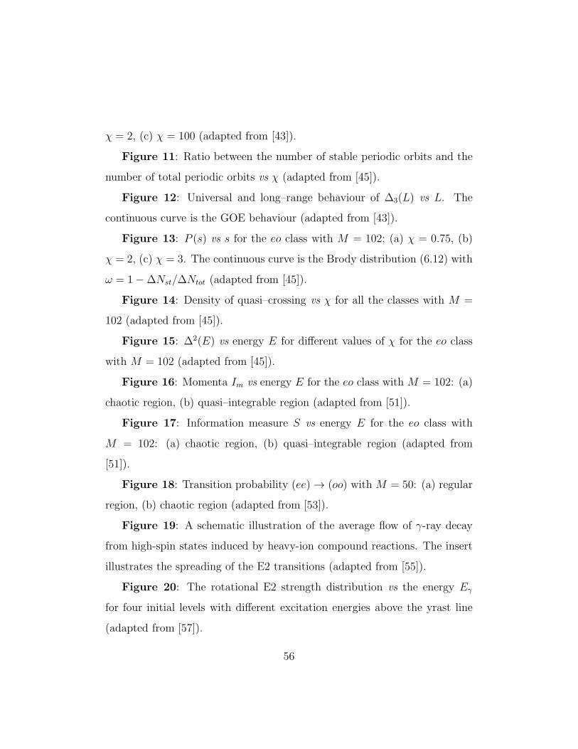
χ = 2, (c) χ = 100 (adapted from [43]).

Figure 11: Ratio between the number of stable periodic orbits and the

number of total periodic orbits vs χ (adapted from [45]).

Figure 12: Universal and long–range behaviour of ∆3(L) vs L. The

continuous curve is the GOE behaviour (adapted from [43]).

Figure 13: P (s) vs s for the eo class with M = 102; (a) χ = 0.75, (b)

χ = 2, (c) χ = 3. The continuous curve is the Brody distribution (6.12) with

ω = 1−∆Nst/∆Ntot (adapted from [45]).

Figure 14: Density of quasi–crossing vs χ for all the classes with M =

102 (adapted from [45]).

Figure 15: ∆2(E) vs energy E for different values of χ for the eo class

with M = 102 (adapted from [45]).

Figure 16: Momenta Im vs energy E for the eo class with M = 102: (a)

chaotic region, (b) quasi–integrable region (adapted from [51]).

Figure 17: Information measure S vs energy E for the eo class with

M = 102: (a) chaotic region, (b) quasi–integrable region (adapted from

[51]).

Figure 18: Transition probability (ee) → (oo) with M = 50: (a) regular

region, (b) chaotic region (adapted from [53]).

Figure 19: A schematic illustration of the average flow of γ-ray decay

from high-spin states induced by heavy-ion compound reactions. The insert

illustrates the spreading of the E2 transitions (adapted from [55]).

Figure 20: The rotational E2 strength distribution vs the energy Eγ

for four initial levels with different excitation energies above the yrast line

(adapted from [57]).

56

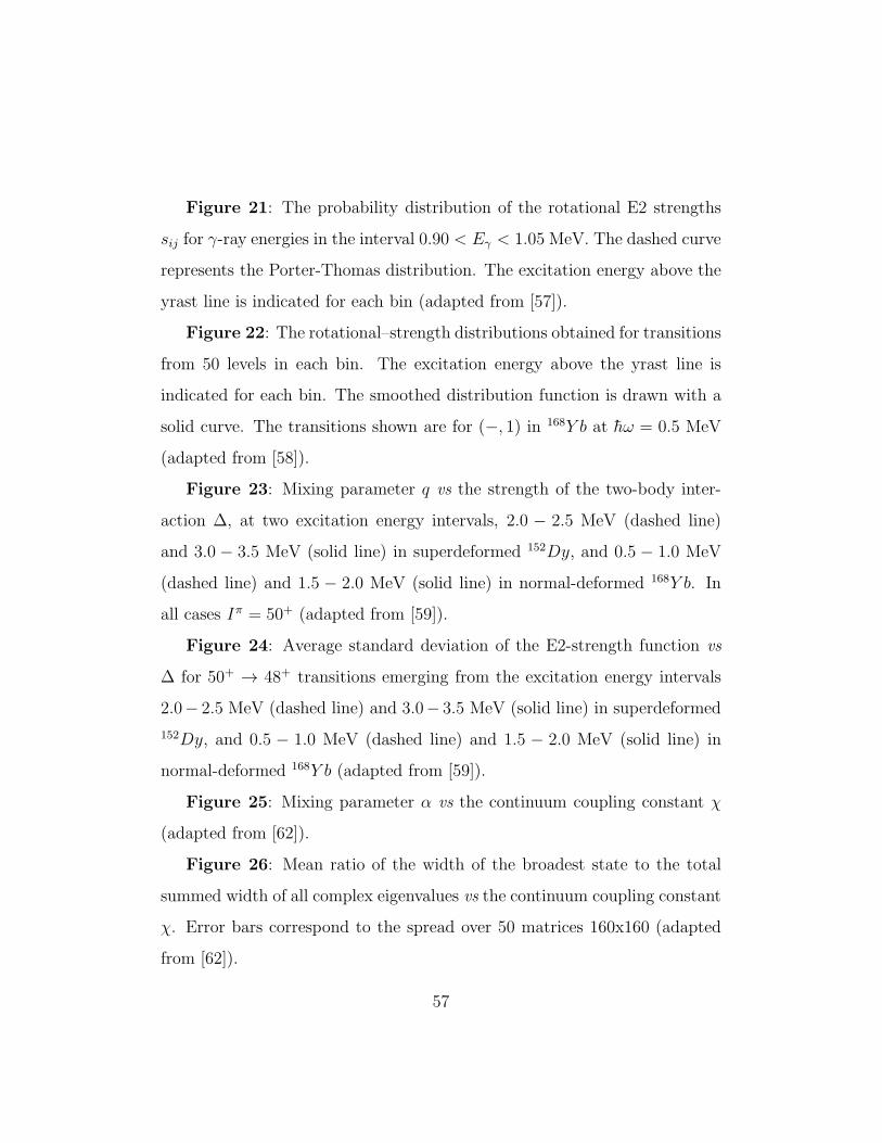
Figure 21: The probability distribution of the rotational E2 strengths

sij for γ-ray energies in the interval 0.90 < Eγ < 1.05 MeV. The dashed curve

represents the Porter-Thomas distribution. The excitation energy above the

yrast line is indicated for each bin (adapted from [57]).

Figure 22: The rotational–strength distributions obtained for transitions

from 50 levels in each bin. The excitation energy above the yrast line is

indicated for each bin. The smoothed distribution function is drawn with a

solid curve. The transitions shown are for (−, 1) in 168Y b at hω = 0.5 MeV

(adapted from [58]).

Figure 23: Mixing parameter q vs the strength of the two-body inter-

action ∆, at two excitation energy intervals, 2.0 − 2.5 MeV (dashed line)

and 3.0 − 3.5 MeV (solid line) in superdeformed 152Dy, and 0.5 − 1.0 MeV

(dashed line) and 1.5 − 2.0 MeV (solid line) in normal-deformed 168Y b. In

all cases Iπ = 50+ (adapted from [59]).

Figure 24: Average standard deviation of the E2-strength function vs

∆ for 50+ → 48+ transitions emerging from the excitation energy intervals

2.0− 2.5 MeV (dashed line) and 3.0− 3.5 MeV (solid line) in superdeformed

152Dy, and 0.5 − 1.0 MeV (dashed line) and 1.5 − 2.0 MeV (solid line) in

normal-deformed 168Y b (adapted from [59]).

Figure 25: Mixing parameter α vs the continuum coupling constant χ

(adapted from [62]).

Figure 26: Mean ratio of the width of the broadest state to the total

summed width of all complex eigenvalues vs the continuum coupling constant

χ. Error bars correspond to the spread over 50 matrices 160x160 (adapted

from [62]).

57

Figure 27: Classical and quantal measures of chaos vs ν (ν = 0: SU(3),

ν = 1: U(5)). Left: λ and σ for angular momentum per boson l = 0.1.

Right: ω and ν for the levels with I = 2+ (adapted from [67]).

58

References

[1] O. BOHIGAS and H.A. WEIDENMULLER: Ann. Rev. Nucl.

Part. Sci., 38, 421 (1988)

[2] P. MARMIER and E. SHELDON: Physics of Nuclei and Par-

ticles, vol. 2 (Academic Press, New York, 1970)

[3] F. IACHELLO and A. ARIMA: The Interacting Boson Model

(Cambridge Univ. Press, Cambridge, 1987)

[4] F. IACHELLO and P. VAN ISACKER: The Interacting Boson–

Fermion Model (Cambridge Univ. Press, Cambridge, 1991)

[5] I. TALMI: Simple Models of Complex Nuclei (Harwood Aca-

demic Press, Paris, 1993)

[6] A. BOHR and B.R. MOTTELSON: Nuclear Structure, vol. 1

(Benjamin, London, 1969)

[7] A. BOHR and B.R. MOTTELSON: Nuclear Structure, vol. 2

(Benjamin, London, 1975)

[8] M.H. MACFARLANE: in Proc.Int. School Enrico Fermi,

Course XL (North–Holand, New York, 1969)

[9] N. BOHR: Nature, 137, 344 (1936)

[10] C.E. PORTER: Statistical Theories of Spectra: Fluctuations,

(Academic Press, 1965)

59

[11] F. DYSON: J. Math. Phys. 3, 140 (1962)

[12] F. DYSON and M. MEHTA: J. Math. Phys. 4, 701 (1963)

[13] E. WIGNER: SIAM Rev. 9, 1 (1967)

[14] M. MEHTA: Random Matrices, II Ed. (Academic Press,

1991)

[15] M. MEHTA: in Statistical Properties of Nuclei, Ed. by J.

GARG (1972)

[16] O. BOHIGAS: in Chaos and Quantum Physics, Les Houches

1989, Ed. M.J. GIANNONI, A. VOROS, and J. ZINN–JUSTIN

(North–Holland, Amsterdam, 1991)

[17] D. BISWASH, S. SINHA and S.V. LAWANDE: Phys. Rev.

A 46, 2649 (1992)

[18] R.U. HAQ, A. PANDEY and O. BOHIGAS: Phys. Rev. Lett.

48, 1086 (1982)

[19] O. BOHIGAS, R.U. HAQ and A. PANDEY: in Nuclear Data

for Science and Technology, Ed. by K.H. BOCKHOFF (1983)

[20] J.D. GARRETT, J.R. GERMAN, L. COURTNEY and J.M.

ESPINO: in Future Directions in Nuclear Physics, pag. 345,

Ed. by J. DUDEK, B. HAAS (American Institute of Physics,

New York, 1992); J.D. GARRETT, J.R. GERMAN: preprint

ORNL/94, submitted to Phys. Rev. Lett.

60

[21] J.F. SHRINER, G.E. MITCHELL and T. VON EGIDY: Z.

Phys. A 338, 309 (1990)

[22] V.I. ARNOLD:Mathematical Methods of Classical Mechanics

(Springer–Verlag, Berlin, 1978); V.I ARNOLD and A. AVEZ:

Ergodic Problem of Classical Mechanics (Benjamin, London,

1968)

[23] M. TABOR: Chaos and Integrability in Non Linear Dynam-

ics, (Wiley, New York, 1989)

[24] O. DE ALMEIDA: Hamiltonian Systems: Chaos and Quan-

tization (Univ. Press, Cambridge, 1990)

[25] M.C. GUTZWILLER: Chaos in Classical and Quantum Me-

chanics (Springer-Verlag, Berlin, 1991)

[26] YA.G. SINAI: Introduction to Ergodic Theory (Univ. Press,

Princeton, 1977)

[27] C. COHEN–TANNOUDJI, B. DIN and F. LALOE: Quantum

Mechanics (1977)

[28] O. BOHIGAS, M. GIANNONI and C. SCHMIT: Phys. Rev.

Lett. 52, 1 (1984)

[29] O. BOHIGAS, M. GIANNONI: in Mathematical and Compu-

tational Methods in Nuclear Physics, Ed. by J.S. DEHESA,

J.M.G. GOMEZ and A. POLLS, Lecture Note in Physics, vol.

61

209 (Springer, Berlin 1984)

[30] M.V. BERRY and M. TABOR: Proc. Roy. Soc. Lond. A

356, 375 (1977)

[31] A. PANDEY, O. BOHIGAS and M.J. GIANNONI: J. Phys.

A 22, 4083 (1989); A. PANDEY and R. RAMASWAMY:

Phys. Rev. A 43, 4237 (1991)

[32] M.C. GUTZWILLER: J. Math. Phys. 11, 1791 (1970)

[33] M.C. GUTZWILLER: J. Math. Phys. 12, 343 (1971)

[34] M. BERRY: Proc. Roy. Soc. Lond. A 400, 229 (1985)

[35] H. LIPKIN, N. MESHKOV and A. GLICK: Nucl. Phys. 62,

188 (1965)

[36] R. WILLIAMS and S. KOONIN: Nucl. Phys. A 391, 72

(1982)

[37] D. MEREDITH, S. KOONIN and M. ZIRNBAUER: Phys.

Rev. A 37, 3499 (1988)

[38] R. GILMORE and H. FENG: Prog. Part. and Nucl. Phys.

9, 479 (1983)

[39] SUBROUTINE D02BAF: The NAG Fortran Library, Mark

14, Oxford: NAG Ltd. and USA: NAG Inc. (1990)

[40] SUBROUTINE E04JAF: The NAG Fortran Library, Mark

62

14, Oxford: NAG Ltd. and USA: NAG Inc. (1990)

[41] M. BARANGER and K. DEVIS: Ann. Phys. 177, 330

(1987); M. DE AGUIAR, C. MALTA, M. BARANGER and

K. DEVIS: Ann. Phys. 180, 167 (1987); M. BARANGER,

K. DEVIS and J. MAHONEY: Ann. Phys. 183, 95 (1988)

[42] H.D. MEYER: J. Chem. Phys. 84, 3147 (1986)

[43] V.R. MANFREDI and L. SALASNICH: Z. Phys. A 343, 1

(1992)

[44] S. ABERG: Prog. Part. Nucl. Phys. 28, 11 (1992)

[45] V.R. MANFREDI, L. SALASNICH and L. DEMATTE: Phys.

Rev. E 47 4556 (1993)

[46] D.W. NOID, M. KOSZYKOWSKI, M. TABOR and R.A.

MARCUS: J. Chem. Phys., 72, 6169 (1980)

[47] R. RAMASWAMY and R.A. MARCUS: J. Chem. Phys. 74,

1385 (1991)

[48] M.V. BERRY: in Chaotic Behaviour in Quantum Mechanics,

pag. 121, Ed. by G. CASATI (Plenum, New York, 1984)

[49] I.C. PERCIVAL: Adv. Chem. Phys., 36, 1 (1977)

[50] L. DEMATTE, V.R. MANFREDI and L. SALASNICH: in

SIF Conference Proc. ’From Classical to Quantum Chaos’,

vol. 41, pag. 111, Ed. by G.F. DELL’ANTONIO, S. FAN-

63

TONI, V.R. MANFREDI (Editrice Compositori, Bologna, 1993)

[51] M.T. LOPEZ–ARIAS and V.R. MANFREDI: Z. Phys. A

334 255 (1989); M.T. LOPEZ–ARIAS, V.R. MANFREDI:

in 3rd Int. Spring Seminar on Nuclear Physics Ed. by A.

COVELLO (1990)

[52] M.V. BERRY: J. Phys. A 10, 2083 (1977); M.V. BERRY,

J.H. HANNAY and A.M. OZORIO DE ALMEIDA: Physica

D 8, 229 (1983)

[53] M.T. LOPEZ–ARIAS and V.R. MANFREDI: Nuovo Ci-

mento A 104, 283 (1991)

[54] D. BAZZACCO: in Int. Conf. on Nuclear Structure at High

Angular Momenta, vol. 2, pag. 376, AECL 10613, Ottawa

(1992)

[55] J.D. GARRETT, G.B. HAGEMANN and B. HERSKIND:

Ann. Rev. Nucl. Part. Sci. 36, 419 (1986)

[56] T. GUHR and H.A. WEIDENMULLER: Ann. Phys. 193,

472 (1989)

[57] M. MATSUO, T. DOSSING, B. HERSKIND and S. FRAUEN-

DORF: Nucl. Phys. A 557, 211c (1993)

[58] M. MATSUO, T. DOSSING, B. HERSKIND and S. FRAUEN-

DORF: Nucl. Phys. A 564, 345 (1993)

64

[59] S. ABERG: Phys. Rev. Lett. 64, 3119 (1990)

[60] T.A. BRODY, J. FLORES, J.B. FRENCH, P.A. MELLO, A.

PANDEY and S.S. WONG: Rev. Mod. Phys. 53, 385 (1981)

[61] V.V. SOKOLOV and V.G. ZELEVINSKY: Nucl. Phys. A

504, 562 (1989)

[62] S. MIZUTORI and V.G. ZELEVINSKY: Z. Phys. A 346, 1

(1993)

[63] J. GINIBRE: J. Math. Phys. 6, 3 (1965)

[64] F. HAAKE: Quantum Signature of Chaos (Springer, Berlin,

1991)

[65] F. HAAKE, F. IZRAILEV, N. LEHMANN, D. SAHER and

H.J. SOMMERS: Z. Phys. B 88, 359 (1992)

[66] R. GROBE, F. HAAKE and H.J. SOMMERS: Phys. Rev.

Lett. 61, 1899 (1988)

[67] N.WHELAN and Y.ALHASSID: Nucl. Phys. A 556, 42

(1993)

65

This figure "fig1-1.png" is available in "png" format from:

http://arxiv.org/ps/nucl-th/9404016v1

This figure "fig2-1.png" is available in "png" format from:

http://arxiv.org/ps/nucl-th/9404016v1

This figure "fig3-1.png" is available in "png" format from:

http://arxiv.org/ps/nucl-th/9404016v1

This figure "fig4-1.png" is available in "png" format from:

http://arxiv.org/ps/nucl-th/9404016v1

This figure "fig5-1.png" is available in "png" format from:

http://arxiv.org/ps/nucl-th/9404016v1

This figure "fig1-2.png" is available in "png" format from:

http://arxiv.org/ps/nucl-th/9404016v1

This figure "fig2-2.png" is available in "png" format from:

http://arxiv.org/ps/nucl-th/9404016v1

This figure "fig3-2.png" is available in "png" format from:

http://arxiv.org/ps/nucl-th/9404016v1

This figure "fig4-2.png" is available in "png" format from:

http://arxiv.org/ps/nucl-th/9404016v1

This figure "fig5-2.png" is available in "png" format from:

http://arxiv.org/ps/nucl-th/9404016v1

This figure "fig1-3.png" is available in "png" format from:

http://arxiv.org/ps/nucl-th/9404016v1

This figure "fig2-3.png" is available in "png" format from:

http://arxiv.org/ps/nucl-th/9404016v1

This figure "fig3-3.png" is available in "png" format from:

http://arxiv.org/ps/nucl-th/9404016v1

This figure "fig4-3.png" is available in "png" format from:

http://arxiv.org/ps/nucl-th/9404016v1

This figure "fig5-3.png" is available in "png" format from:

http://arxiv.org/ps/nucl-th/9404016v1

This figure "fig1-4.png" is available in "png" format from:

http://arxiv.org/ps/nucl-th/9404016v1

This figure "fig2-4.png" is available in "png" format from:

http://arxiv.org/ps/nucl-th/9404016v1

This figure "fig3-4.png" is available in "png" format from:

http://arxiv.org/ps/nucl-th/9404016v1

This figure "fig4-4.png" is available in "png" format from:

http://arxiv.org/ps/nucl-th/9404016v1

This figure "fig5-4.png" is available in "png" format from:

http://arxiv.org/ps/nucl-th/9404016v1

This figure "fig1-5.png" is available in "png" format from:

http://arxiv.org/ps/nucl-th/9404016v1

This figure "fig2-5.png" is available in "png" format from:

http://arxiv.org/ps/nucl-th/9404016v1

This figure "fig3-5.png" is available in "png" format from:

http://arxiv.org/ps/nucl-th/9404016v1

This figure "fig4-5.png" is available in "png" format from:

http://arxiv.org/ps/nucl-th/9404016v1