Journal of Testing and Evaluation, Vol. 38, No. 2Paper ID JTE101907

Available online at: www.astm.org

CoDoNa

J. R. Mohanty,1 B. B. Verma,2 P. K. Ray,3 and D. R. K Parhi3

Application of Artificial Neural Network for FatigueLife Prediction under Interspersed Mode-I SpikeOverload

ABSTRACT: The objective of this study is to design multi-layer perceptron artificial neural network (ANN) architecture in order to predict thefatigue life along with different retardation parameters under constant amplitude loading interspersed with mode-I overload. Fatigue crack growthtests were conducted on two aluminum alloys 7020-T7 and 2024-T3 at various overload ratios using single edge notch tension specimens. Theexperimental data sets were used to train the proposed ANN model to predict the output for new input data sets (not included in the training sets). Themodel results were compared with experimental data and also with Wheeler’s model. It was observed that the model slightly over-predicts the fatiguelife with maximum error of + 4.0 % under the tested loading conditions

KEYWORDS: artificial neural network, overload ratio, multi-layer perceptron, retardation parameters

Nomenclature

a = crack length measured from edge of thespecimen (mm)

ai = crack length corresponding to the ith step (mm)aj = crack length corresponding to the jth step (mm)

aol = crack length at overload (mm)ad = retarded crack length (mm)ad

A = retarded (ANN) crack length (mm)ad

E = retarded (experimental) crack length (mm)ad

W = retarded (Wheeler) crack length (mm)B = plate thickness (mm)C = constant in the Paris equation

COD = crack opening displacementCGR = crack growth rate�Cp�i = retardation parameter

da /dN = crack growth rate (mm/cycle)�da /dN�retarded= retarded crack growth rate (mm/cycle)

E = modulus of elasticity (MPa)Err = sum-squared error

f�g� = geometrical factorf� . � = activation function

F = remotely applied load (N)K = stress intensity factor �MPa�m�

KIC = plane strain fracture toughness �MPa�m�Kmax = maximum stress intensity factor �MPa�m�Kmax

B = maximum (base line) stress intensity factor�MPa�m�

Manuscript received May 29, 2008; accepted for publication September 7,2009; published online October 2009.

1Dept. of Metallurgical and Materials Engineering, National Institute ofTechnology, Rourkela 769008, India (Corresponding author), e-mail:guddy95@yahoomail.co.in; guddy95@gmail.com

2Dept. of Metallurgical and Materials Engineering, National Institute ofTechnology, Rourkela 769008, India.

3Dept. of Mechanical Engineering, National Institute of Technology, Rour-

kela 769008, India.

Copyright © 2010 by ASTM International, 100 Barr Harbor Drive, PO Box C700, Wpyright by ASTM Int'l (all rights reserved); Mon Mar 29 06:13:57 EDT 2010wnloaded/printed bytional Institute of Technology Rourkela pursuant to License Agreement. No further

Kol = stress intensity factor at overload �MPa�m��K = stress intensity factor range �MPa�m�lay = layer number

MSIF = maximum stress intensity factorn = exponent in the Paris equationN = number of cycles or fatigue life

Nd = number of delay cycleNd

A = number of delay cycle (ANN)Nd

E = number of delay cycle (experimental)Nd

W = number of delay cycle (Wheeler)Nf

A = final number of cycles (ANN)Nf

E = final number of cycles (experimental)OLR = overload ratio

p = shaping exponent in the Wheeler modelr = label for rth neuron in hidden layer lay-1

rpi = current plastic zone size corresponding to theith cycle (mm)

rpo = overload plastic zone size (mm)Rol = overload load ratio

s = label for sth neuron in the hidden layer laySIFR = stress intensity factor range

t = iteration numberw = plate width (mm)

Wsr�lay� = weight of the connection from neuron r in layer

lay-1 to neuron s in layer layy1 ,y2 ,y3 = inputs to the ANN

� = retardation correction factor� = plastic zone correction factor� = Poison’s ratio� = momentum coefficient� = learning rate

�s�lay� = local error gradient�ys = yield point stress (MPa)�ut = ultimate stress (MPa)

est Conshohocken, PA 19428-2959. 1

reproductions authorized.

2 JOURNAL OF TESTING AND EVALUATION

CoDoNa

Introduction

Most load bearing structural components are subjected to randomloading in service consisting of distinguished peaks. These loadcycle interactions can have a very significant effect on the fatiguecrack propagation, which is a path dependent process [1]. A tensileoverload can retard or even arrest the growing fatigue crack, whilea compressive under load can accelerate it [2–8]. Overload-inducedretardation has a significant effect on fatigue crack growth as it en-hances the life of the structure. A number of mechanisms may beresponsible to explain the crack retardation phenomena, includingplasticity induced crack-closure, blunting, and/or bifurcation of thecrack-tip, residual stresses and strains, strain-hardening, crack-faceroughness, oxidation of crack faces, etc. [5,6,9–14]. However, fordesign purposes it is particularly difficult to generate a universalalgorithm to quantify these sequence effects on fatigue crackgrowth due to the number and to the complexity of the mechanismsinvolved in this problem [15]. Irrespective of significant ambiguityand disagreements as regards to the exact mechanism of retarda-tion, a number of empirical models [16] have been proposed. But, atechnological gap still exists in the automatic prediction of fatiguelife in the case of mode-I spike load. This can be accomplished bythe use of artificial neural network (ANN).

ANN is a new class of computational intelligence system that isuseful to handle various complex problems with a capacity to learnby examples. The first ANN concept was adopted by McCullochand Pits [17] in 1943, who suggested the cell model. Althoughsome pioneer work was undertaken in 1949 [18] by focusing atten-tion on the learning system of human brain, the actual developmenton ANN concept started towards 1980 through various studies [19].It has emerged as a new field of soft-computing to deal with manymultivariate complex problems for which an accurate analyticalmodel does not exist [20–22]. ANN has proven to be a powerful andversatile computational tool in the application of a number of engi-neering fields [23–28]. In recent years, ANN has been also intro-duced in the field of fatigue in order to predict fatigue life [29–35].A brief review on the topic has been presented by Jia et al. [36].They used ANN to predict valuable fatigue responses in order tofacilitate the development of design guidelines for hybrid materialbonded interfaces.

In this study, ANN has been used to predict fatigue CGR(FCGR) under mode-I spike load with various overload ratio(OLR) �Rol�. The simulated results of unknown load ratio (not in-cluded in the training set (TS)) have been utilized to calculate theretardation parameters (ad and Nd) as well as the residual life. Thepredicted results have been compared with the experimental dataconducted on 7020-T7 and 2024-T3 Al alloys. It is observed thatthe results are in good agreement with the experimental findings.

Experimental Procedure

The fatigue tests were performed on 7020-T7 and 2024-T3 alumi-num alloys using single edge notched tension specimens having athickness of 6.5 mm. The chemical composition and the mechani-cal properties of the alloys are given in Tables 1 and 2, respectively.

TABLE 1—Chem

Materials Al Cu Mg Mn

7020-T7 93.13 0.05 1.2 0.43

2024-T3 92.78 3.9 1.5 0.32

pyright by ASTM Int'l (all rights reserved); Mon Mar 29 06:13:57 EDT 2010wnloaded/printed bytional Institute of Technology Rourkela pursuant to License Agreement. No further

The specimens were made in the longitudinal transverse directionfrom the plate.

All the experiments were conducted in ambient temperature ona servo-hydraulic dynamic testing machine (Instron-8502) with250 kN load cell interfaced to a computer. The test specimens werefatigue pre-cracked under mode-I loading to an a /w ratio of 0.3 andwere subjected to constant load amplitude test (i.e., progressive in-crease in �K with crack extension) maintaining a load ratio of 0.1.The sinusoidal loads were applied at a frequency of 6 Hz. The crackgrowth was monitored with the help of a crack opening displace-ment gauge mounted on the face of the machined notch. The stressintensity factor K was calculated using equations proposed byBrown and Srawley [37] as follows:

K = f�g� ·F�a

wB(1)

where

f�g� = 1.12 − 0.231�a/w� + 10.55�a/w�2 − 21.72�a/w�3

+ 30.39�a/w�4 (2)

The fatigue crack growth test was continued up to an a /w ratioof 0.4, and then a mode-I spike (static) overload was applied. Afterthe application of overload, the pre-overload fatigue crack growthtest (i.e., constant amplitude loading at load ratio of 1.0) was con-tinued till the specimen fractured. The overloading was done at aloading rate of 8.0 kN/min at different OLRs such as 2.0, 2.25,2.35, 2.5, 2.6, and 2.75 for six 7020 T7 Al-alloy specimens and 1.5,1.75, 2.0, 2.1, 2.25, and 2.5 for six 2024 T3 Al-alloy specimens. TheOLR is defined as

Rol =Kol

KmaxB (3)

where KmaxB is the maximum stress intensity factor (MSIF) for base

line test.

Artificial Neural Network

Fundamental Approach

The term “neural network” refers to a collection of neurons, theirconnections, and the connection strengths between them. Theknowledge is acquired during the training process by correcting thecorresponding weights so as to minimize an error function. Thereare three types of learning in ANN technology: Supervised, unsu-pervised, and reinforcement. In the case of supervised learning(learning with a teacher), the network is trained by optimizing cor-responding weights in such a way that the significant outputs can beobtained for the inputs not belonging to the TS. The unsupervisedtraining is based on organizing the structure so that similar stimuliactivate similar neurons where there is no pre-defined output andthe network finds differences and affinities between the inputs. Thereinforcement learning, which is a particular form of supervised

composition.

Fe Si Zn Cr Others

0.37 0.22 4.6 ¯ ¯

0.5 0.5 0.25 0.1 0.15

ical

reproductions authorized.

MOHANTY ET AL. ON FATIGUE LIFE PREDICTION BY ANN 3

CoDoNa

training, attempts to learn input-output vectors by trial and errorthrough maximizing a performance function (named reinforcementsignal).

Back propagation networks are in fact the powerful networksthat refer to a multi-layered feed-forward perceptron trained withan error back propagation algorithm (error minimization tech-nique). The architecture of a simple back propagation ANN is acollection of nodes distributed over a layer of input neurons, one ormore layers of hidden neurons, and a layer of output neurons. Neu-rons in each layer are interconnected to subsequent layer neuronswith links, each of which carries a weight that describes thestrength of that connection. Various non-linear activation functions,such as sigmoidal, tanh or radial (Gaussian), are used to model theneuron activity. Inputs are propagated forward through each layerof the network to emerge as outputs. The errors between those out-puts and the target (desired output) are then propagated backwardthrough the network, and then connection weights are adjusted soas to minimize the error.

Design and Analysis of ANN Model for CrackGrowth Rate Prediction

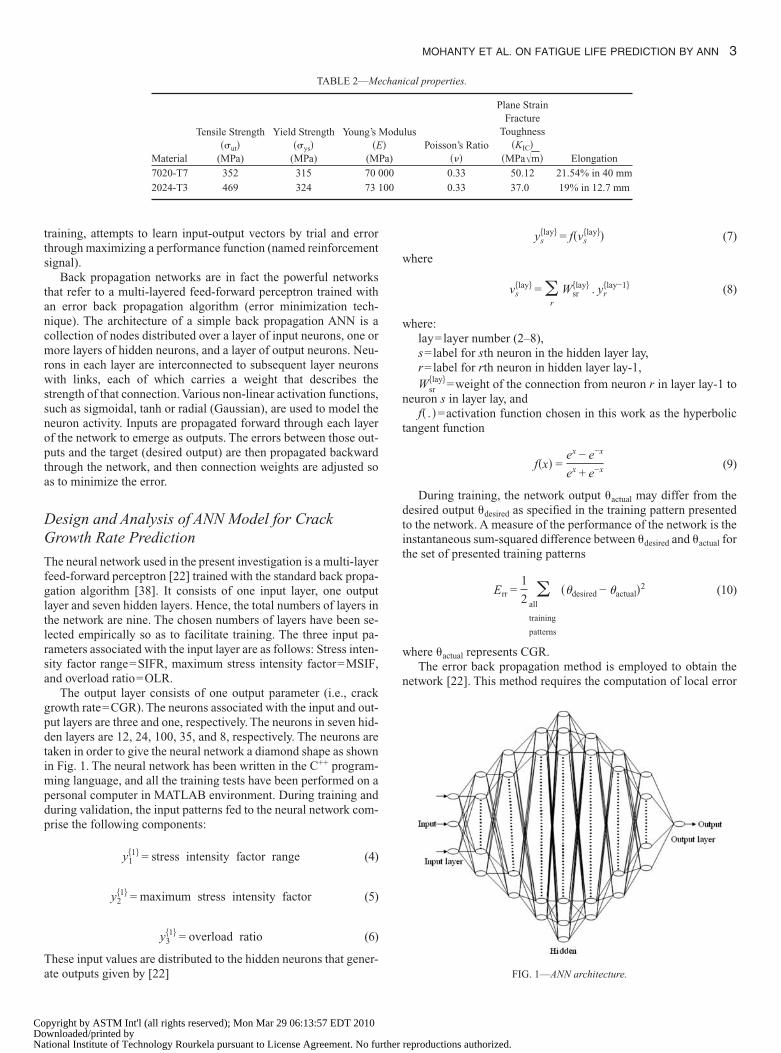
The neural network used in the present investigation is a multi-layerfeed-forward perceptron [22] trained with the standard back propa-gation algorithm [38]. It consists of one input layer, one outputlayer and seven hidden layers. Hence, the total numbers of layers inthe network are nine. The chosen numbers of layers have been se-lected empirically so as to facilitate training. The three input pa-rameters associated with the input layer are as follows: Stress inten-sity factor range=SIFR, maximum stress intensity factor=MSIF,and overload ratio=OLR.

The output layer consists of one output parameter (i.e., crackgrowth rate=CGR). The neurons associated with the input and out-put layers are three and one, respectively. The neurons in seven hid-den layers are 12, 24, 100, 35, and 8, respectively. The neurons aretaken in order to give the neural network a diamond shape as shownin Fig. 1. The neural network has been written in the C++ program-ming language, and all the training tests have been performed on apersonal computer in MATLAB environment. During training andduring validation, the input patterns fed to the neural network com-prise the following components:

y1�1� = stress intensity factor range (4)

y2�1� = maximum stress intensity factor (5)

y3�1� = overload ratio (6)

These input values are distributed to the hidden neurons that gener-

TABLE 2—Me

Material

Tensile Strength��ut�

(MPa)

Yield Strength��ys�

(MPa)

Young’s M�E

(MP

7020-T7 352 315 70 0

2024-T3 469 324 73 1

ate outputs given by [22]

pyright by ASTM Int'l (all rights reserved); Mon Mar 29 06:13:57 EDT 2010wnloaded/printed bytional Institute of Technology Rourkela pursuant to License Agreement. No further

ys�lay� = f�vs

�lay�� (7)

where

vs�lay� = �

r

Wsr�lay� . yr

�lay−1� (8)

where:lay=layer number (2–8),s=label for sth neuron in the hidden layer lay,r=label for rth neuron in hidden layer lay-1,Wsr

�lay�=weight of the connection from neuron r in layer lay-1 toneuron s in layer lay, and

f� . �=activation function chosen in this work as the hyperbolictangent function

f�x� =ex − e−x

ex + e−x (9)

During training, the network output actual may differ from thedesired output desired as specified in the training pattern presentedto the network. A measure of the performance of the network is theinstantaneous sum-squared difference between desired and actual forthe set of presented training patterns

Err =1

2 �all

training

patterns

�desired − actual�2 (10)

where actual represents CGR.The error back propagation method is employed to obtain the

network [22]. This method requires the computation of local error

ical properties.

lusPoisson’s Ratio

���

Plane StrainFracture

Toughness�KIC�

�MPa�m� Elongation

0.33 50.12 21.54% in 40 mm

0.33 37.0 19% in 12.7 mm

chan

odu�a)

00

00

FIG. 1—ANN architecture.

reproductions authorized.

4 JOURNAL OF TESTING AND EVALUATION

CoDoNa

gradients in order to determine appropriate weight corrections toreduce Err. For the output layer, the error gradient ��9� is

��9� = f��V19��desired − actual� (11)

The local gradient for neurons in hidden layer {lay} is given by

�s�lay� = f��Vs

�lay����k

�k�lay+1�Wks

�lay+1�� (12)

The synaptic weights are updated according to the following ex-pressions:

Wsr�t + 1� = Wsr�t� + �Wsr�t + 1� (13)

and

�Wsr�t + 1� = ��Wsr�t� + ��s�lay�yr

�lay−1� (14)

where�=momentum coefficient (chosen empirically as 0.2 in this

work),�=learning rate (chosen empirically as 0.35 in this work), andt=iteration number, each iteration consisting of the presentation

of a training pattern and correction of the weights.The final output from the neural network is

actual = f�V1�9�� (15)

where

V1�9� = �

r

W1r�9�yr

�8� (16)

Application of Neural Network Architecture

Proper selection of input and output parameters and their normal-ization are the two primary objectives to design a suitable ANNarchitecture. The proposed ANN model has been developed usingback propagation architecture with three inputs and one output. Thetwo crack driving forces, SIFR ��K� and MSIF �Kmax�, have beenchosen as the two inputs. The selection of �K and Kmax as two in-puts for the present model is based on the principle of unified ap-proach [5,39,40]. According to this principle, fatigue is consideredas two-parametric problem because there are two driving forces(�K and Kmax) required to obtain fatigue crack growth. The thirdinput is the OLR �Rol� as the amount of retardation varies with theOLR. CGR �da� /dN� � has been selected as the output for the presentstudy. As far as normalization of input and output parameters areconcerned, classical normalization, where the range is scaled be-tween zero and one, may not be applicable in every ANN model. Tomake the input amenable for successful learning to minimize theoverall sum-squared error, the two input parameters �K and Kmax

have been normalized between one and four, while the other one,OLR �Rol�, has been normalized between one and three. Similarlythe output �da /dN� has been normalized between zero and three fornetwork training and testing. The inputs and outputs of the TSs have

TABLE 3—Performance of

MaterialMomentumCoefficient

LearningRate

HiddenNeurons

7020-T7 0.2 0.35 179

2024-T3 0.2 0.35 179

been constituted from 50�50�50 experimental values of �K,

pyright by ASTM Int'l (all rights reserved); Mon Mar 29 06:13:57 EDT 2010wnloaded/printed bytional Institute of Technology Rourkela pursuant to License Agreement. No further

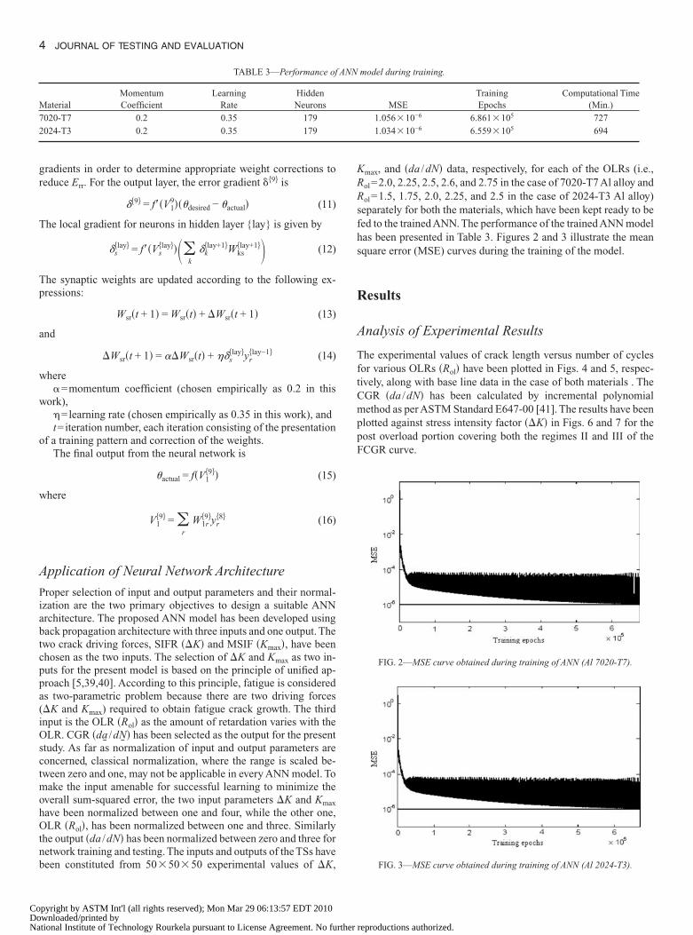
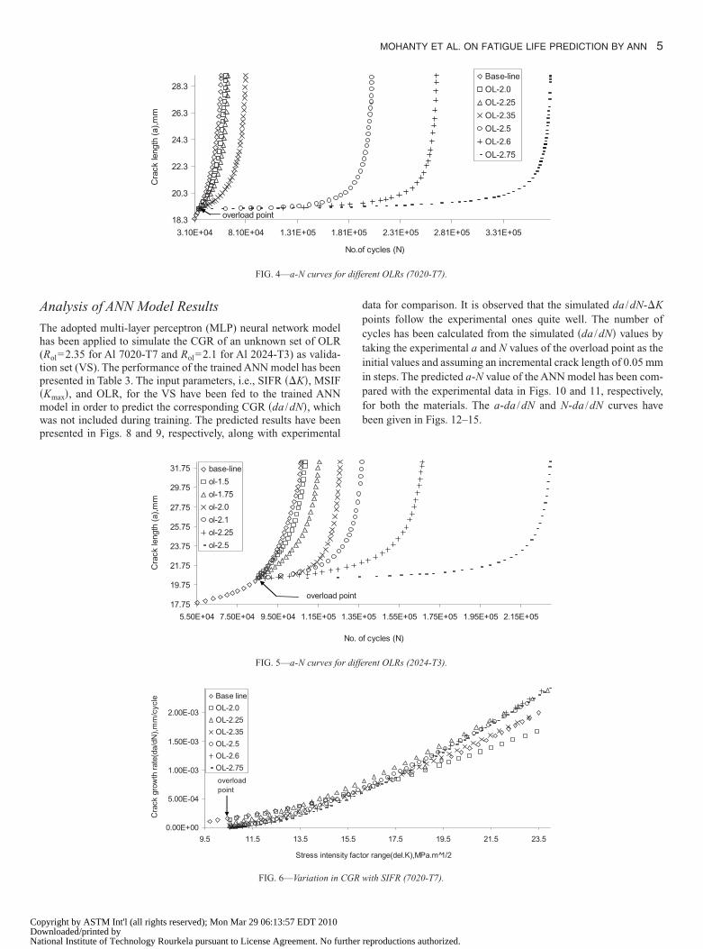
Kmax, and �da /dN� data, respectively, for each of the OLRs (i.e.,Rol=2.0, 2.25, 2.5, 2.6, and 2.75 in the case of 7020-T7 Al alloy andRol=1.5, 1.75, 2.0, 2.25, and 2.5 in the case of 2024-T3 Al alloy)separately for both the materials, which have been kept ready to befed to the trained ANN. The performance of the trained ANN modelhas been presented in Table 3. Figures 2 and 3 illustrate the meansquare error (MSE) curves during the training of the model.

Results

Analysis of Experimental Results

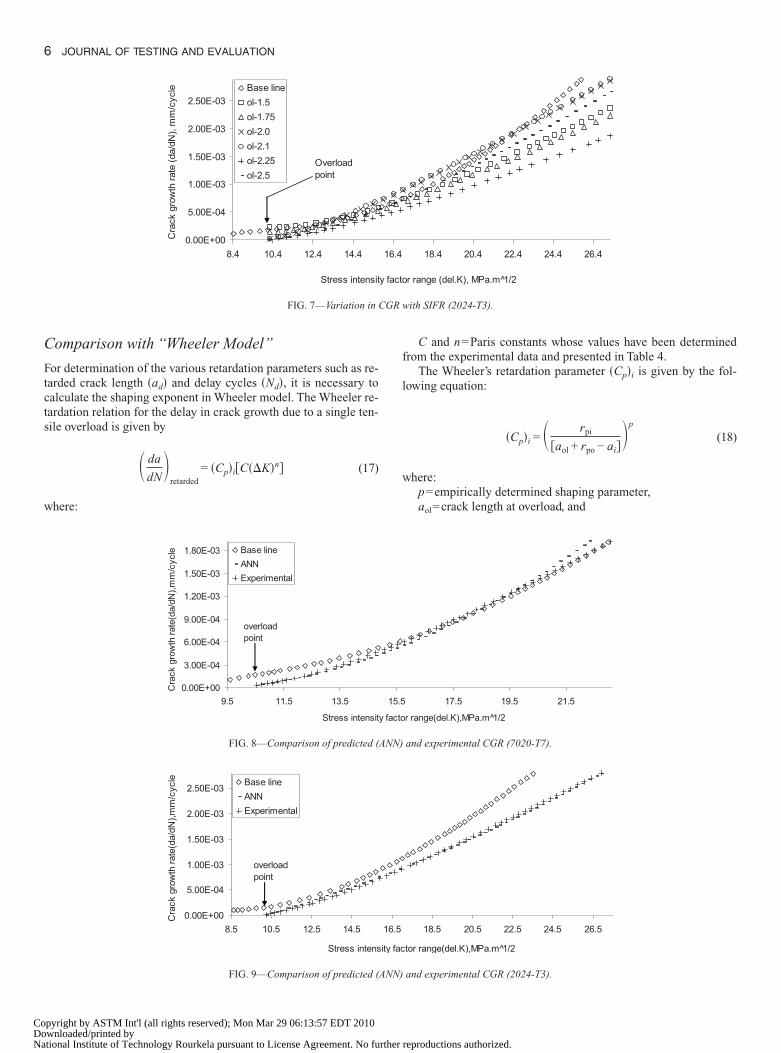
The experimental values of crack length versus number of cyclesfor various OLRs �Rol� have been plotted in Figs. 4 and 5, respec-tively, along with base line data in the case of both materials . TheCGR �da /dN� has been calculated by incremental polynomialmethod as per ASTM Standard E647-00 [41]. The results have beenplotted against stress intensity factor ��K� in Figs. 6 and 7 for thepost overload portion covering both the regimes II and III of theFCGR curve.

model during training.

MSETrainingEpochs

Computational Time(Min.)

1.056�10−6 6.861�105 727

1.034�10−6 6.559�105 694

FIG. 2—MSE curve obtained during training of ANN (Al 7020-T7).

ANN

FIG. 3—MSE curve obtained during training of ANN (Al 2024-T3).

reproductions authorized.

r diffe

MOHANTY ET AL. ON FATIGUE LIFE PREDICTION BY ANN 5

CoDoNa

Analysis of ANN Model Results

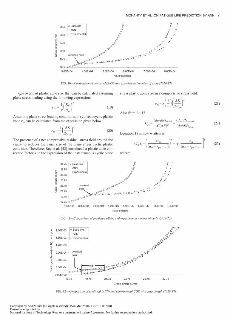
The adopted multi-layer perceptron (MLP) neural network modelhas been applied to simulate the CGR of an unknown set of OLR(Rol=2.35 for Al 7020-T7 and Rol=2.1 for Al 2024-T3) as valida-tion set (VS). The performance of the trained ANN model has beenpresented in Table 3. The input parameters, i.e., SIFR ��K�, MSIF�Kmax�, and OLR, for the VS have been fed to the trained ANNmodel in order to predict the corresponding CGR �da /dN�, whichwas not included during training. The predicted results have beenpresented in Figs. 8 and 9, respectively, along with experimental

18.3

20.3

22.3

24.3

26.3

28.3

3.10E+04 8.10E+04 1.31E+05 1.8

Cracklength(a),mm

overload point

FIG. 4—a-N curves fo

17.75

19.75

21.75

23.75

25.75

27.75

29.75

31.75

5.50E+04 7.50E+04 9.50E+04 1.15E+05

Cracklength(a),mm

base-lineol-1.5ol-1.75ol-2.0ol-2.1ol-2.25ol-2.5

overload p

FIG. 5—a-N curves fo

0.00E+00

5.00E-04

1.00E-03

1.50E-03

2.00E-03

9.5 11.5 13.5 1

Stress intensi

Crackgrowthrate(da/dN),mm/cycle Base line

OL-2.0OL-2.25OL-2.35OL-2.5OL-2.6OL-2.75overloadpoint

FIG. 6—Variation in CGR

pyright by ASTM Int'l (all rights reserved); Mon Mar 29 06:13:57 EDT 2010wnloaded/printed bytional Institute of Technology Rourkela pursuant to License Agreement. No further

data for comparison. It is observed that the simulated da /dN-�Kpoints follow the experimental ones quite well. The number ofcycles has been calculated from the simulated �da /dN� values bytaking the experimental a and N values of the overload point as theinitial values and assuming an incremental crack length of 0.05 mmin steps. The predicted a-N value of the ANN model has been com-pared with the experimental data in Figs. 10 and 11, respectively,for both the materials. The a-da /dN and N-da /dN curves havebeen given in Figs. 12–15.

5 2.31E+05 2.81E+05 3.31E+05

f cycles (N)

Base-lineOL-2.0OL-2.25OL-2.35OL-2.5OL-2.6OL-2.75

rent OLRs (7020-T7).

+05 1.55E+05 1.75E+05 1.95E+05 2.15E+05

f cycles (N)

rent OLRs (2024-T3).

17.5 19.5 21.5 23.5

or range(del.K),MPa.m 1̂/2

1E+0

No.o

1.35E

No. o

oint

r diffe

5.5

ty fact

with SIFR (7020-T7).

reproductions authorized.

GR

6 JOURNAL OF TESTING AND EVALUATION

CoDoNa

Comparison with “Wheeler Model”

For determination of the various retardation parameters such as re-tarded crack length �ad� and delay cycles �Nd�, it is necessary tocalculate the shaping exponent in Wheeler model. The Wheeler re-tardation relation for the delay in crack growth due to a single ten-sile overload is given by

� da

dN�

retarded

= �Cp�iC��K�n (17)

where:

0.00E+00

5.00E-04

1.00E-03

1.50E-03

2.00E-03

2.50E-03

8.4 10.4 12.4 14.4

Stress intensit

Crackgrowthrate(da/dN),mm/cycle Base line

ol-1.5ol-1.75ol-2.0ol-2.1ol-2.25ol-2.5

Overloadpoint

FIG. 7—Variation in C

0.00E+00

3.00E-04

6.00E-04

9.00E-04

1.20E-03

1.50E-03

1.80E-03

9.5 11.5 13.5

Stress intensity

Crackgrowthrate(da/dN),mm/cycle Base line

ANNExperimental

overloadpoint

FIG. 8—Comparison of predicted (A

0.00E+00

5.00E-04

1.00E-03

1.50E-03

2.00E-03

2.50E-03

8.5 10.5 12.5 14.5

Stress intens

Crackgrowthrate(da/dN),mm/cycle Base line

ANNExperimental

overloadpoint

FIG. 9—Comparison of predicted (ANN)

pyright by ASTM Int'l (all rights reserved); Mon Mar 29 06:13:57 EDT 2010wnloaded/printed bytional Institute of Technology Rourkela pursuant to License Agreement. No further

C and n=Paris constants whose values have been determinedfrom the experimental data and presented in Table 4.

The Wheeler’s retardation parameter �Cp�i is given by the fol-lowing equation:

�Cp�i = � rpi

aol + rpo − ai�p

(18)

where:p=empirically determined shaping parameter,aol=crack length at overload, and

18.4 20.4 22.4 24.4 26.4

or range (del.K), MPa.m 1̂/2

with SIFR (2024-T3).

17.5 19.5 21.5

r range(del.K),MPa.m 1̂/2

and experimental CGR (7020-T7).

18.5 20.5 22.5 24.5 26.5

tor range(del.K),MPa.m 1̂/2

16.4

y fact

15.5

facto

NN)

16.5

ity fac

and experimental CGR (2024-T3).

reproductions authorized.

) and

MOHANTY ET AL. ON FATIGUE LIFE PREDICTION BY ANN 7

CoDoNa

rpo=overload plastic zone size that can be calculated assumingplane stress loading using the following expression:

rpo =1

�Kol

�ys�2

(19)

Assuming plane stress loading conditions, the current cyclic plasticzone rpi can be calculated from the expression given below

rpi =1

� �K

2�ys�2

(20)

The presence of a net compressive residual stress field around thecrack-tip reduces the usual size of the plane stress cyclic plasticzone size. Therefore, Ray et al. [42] introduced a plastic zone cor-rection factor � in the expression of the instantaneous cyclic plane

18.3

20.3

22.3

24.3

26.3

28.3

3.00E+04 4.00E+04 5.00E+04

Cracklength(a),mm

Base lineANNExperimental

overload point

FIG. 10—Comparison of predicted (ANN

17.75

19.75

21.75

23.75

25.75

27.75

29.75

31.75

7.00E+04 8.00E+04 9.00E+04 1.00E

N

Cracklength(a),mm

Base lineANNExperimental

overloadpoint

FIG. 11—Comparison of predicted (ANN

0.00E+00

3.00E-04

6.00E-04

9.00E-04

1.20E-03

1.50E-03

1.80E-03

17.75 19.75 21.75

Crackgrowthrate(da/dN),mm/cycle Base line

ANNExperimental

ad

overloadpoint

FIG. 12—Comparison of predicted (ANN) and exp

pyright by ASTM Int'l (all rights reserved); Mon Mar 29 06:13:57 EDT 2010wnloaded/printed bytional Institute of Technology Rourkela pursuant to License Agreement. No further

stress plastic zone size in a compressive stress field.

rpi = �� 1

�� �K

2�ys�2

(21)

Also from Eq 17

Cpi=

�da/dN�retard

C��K�n =�da/dN�retard

�da/dN�a=a0

(22)

Equation 18 is now written as

�Cp�i = � �rpi

aol + rpo − ai�p

= �� rpi

�aol + rpo − ai��p

(23)

where:

6.00E+04 7.00E+04 8.00E+04

cycle(N)

experimental number of cycle (7020-T7)

1.10E+05 1.20E+05 1.30E+05 1.40E+05

ycle(N)

experimental number of cycle (2024-T3).

23.75 25.75 27.75

length(a),mm

No. of

+05

o.of c

) and

Crack

erimental CGR with crack length (7020-T7).

reproductions authorized.

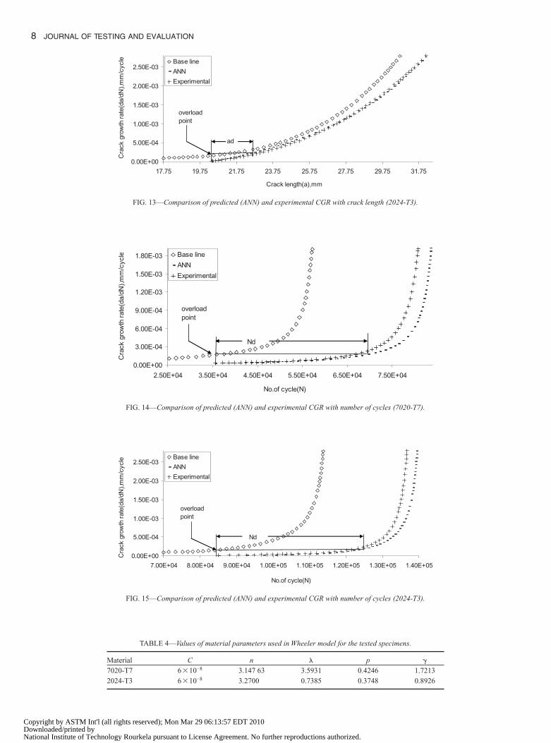
FIG. 13—Comparison of predicted (ANN) and experimental CGR with crack length (2024-T3).

FIG. 15—Comparison of predicted (ANN) and experimental CGR with number of cycles (2024-T3).

8 JOURNAL OF TESTING AND EVALUATION

CoDoNa

TABLE 4—Values of material parameters used in Wheeler model for the tested specimens.

Material C n � p �

7020-T7 6�10−8 3.147 63 3.5931 0.4246 1.7213

2024-T3 6�10−8 3.2700 0.7385 0.3748 0.8926

0.00E+00

5.00E-04

1.00E-03

1.50E-03

2.00E-03

2.50E-03

17.75 19.75 21.75 23.75 25.75 27.75 29.75 31.75

Crack length(a),mm

Crackgrowthrate(da/dN),mm/cycle Base line

ANNExperimental

ad

overloadpoint

0.00E+00

3.00E-04

6.00E-04

9.00E-04

1.20E-03

1.50E-03

1.80E-03

2.50E+04 3.50E+04 4.50E+04 5.50E+04 6.50E+04 7.50E+04

No.of cycle(N)

Crackgrowthrate(da/dN),mm/cycle Base line

ANNExperimental

Nd

overloadpoint

FIG. 14—Comparison of predicted (ANN) and experimental CGR with number of cycles (7020-T7).

0.00E+00

5.00E-04

1.00E-03

1.50E-03

2.00E-03

2.50E-03

7.00E+04 8.00E+04 9.00E+04 1.00E+05 1.10E+05 1.20E+05 1.30E+05 1.40E+05

No.of cycle(N)

Crackgrowthrate(da/dN),mm/cycle Base line

ANNExperimental

Nd

overloadpoint

pyright by ASTM Int'l (all rights reserved); Mon Mar 29 06:13:57 EDT 2010wnloaded/printed bytional Institute of Technology Rourkela pursuant to License Agreement. No further reproductions authorized.

NN),

MOHANTY ET AL. ON FATIGUE LIFE PREDICTION BY ANN 9

CoDoNa

�=correction factor, which is expressed as �=�p.The values of �, �, and p calculated using Eqs 22 and 23 are

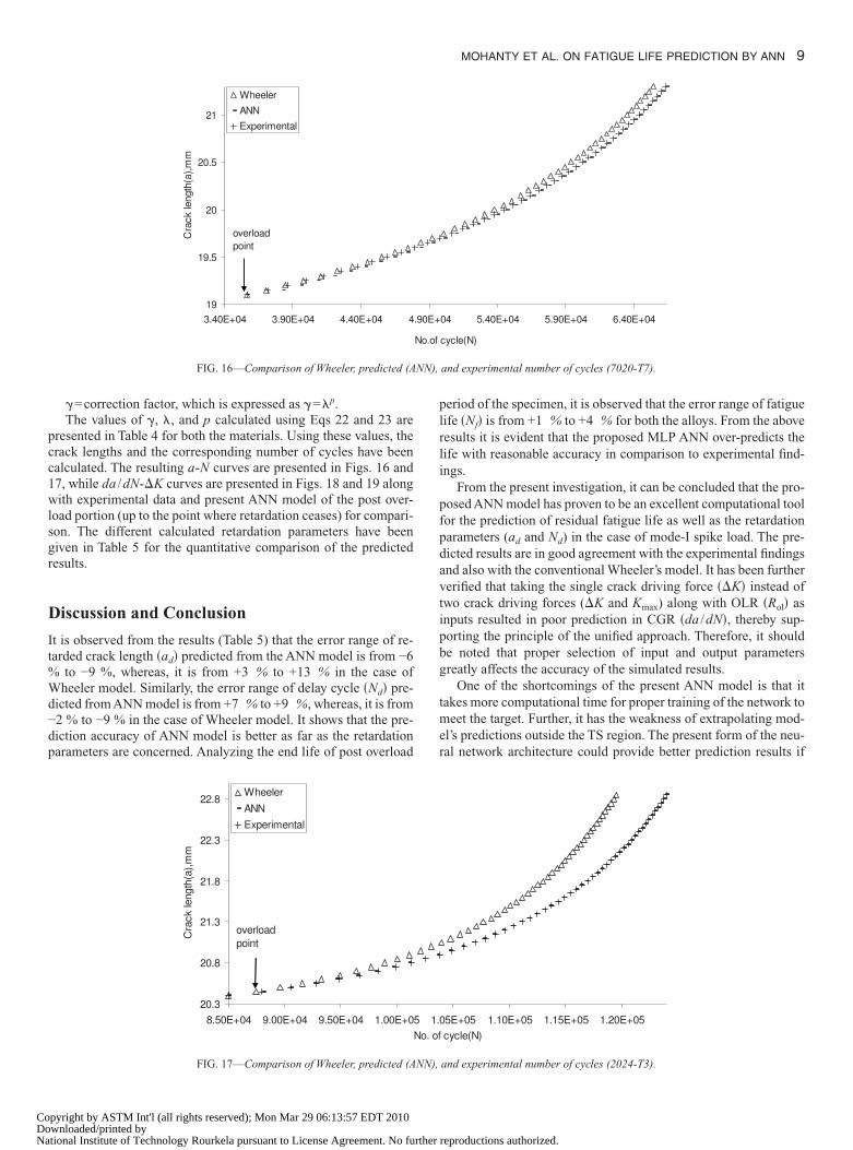
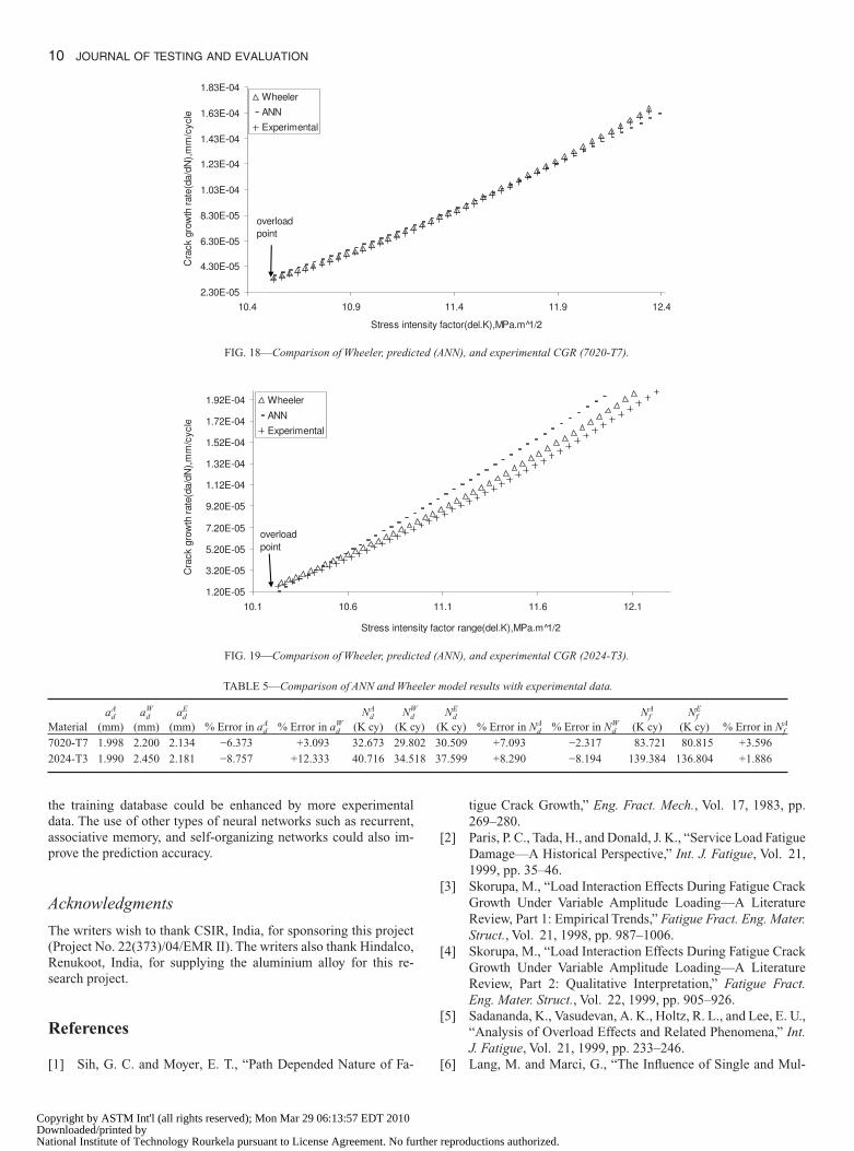
presented in Table 4 for both the materials. Using these values, thecrack lengths and the corresponding number of cycles have beencalculated. The resulting a-N curves are presented in Figs. 16 and17, while da /dN-�K curves are presented in Figs. 18 and 19 alongwith experimental data and present ANN model of the post over-load portion (up to the point where retardation ceases) for compari-son. The different calculated retardation parameters have beengiven in Table 5 for the quantitative comparison of the predictedresults.

Discussion and Conclusion

It is observed from the results (Table 5) that the error range of re-tarded crack length �ad� predicted from the ANN model is from −6% to −9 %, whereas, it is from +3 % to +13 % in the case ofWheeler model. Similarly, the error range of delay cycle �Nd� pre-dicted from ANN model is from +7 % to +9 %, whereas, it is from−2 % to −9 % in the case of Wheeler model. It shows that the pre-diction accuracy of ANN model is better as far as the retardationparameters are concerned. Analyzing the end life of post overload

19

19.5

20

20.5

21

3.40E+04 3.90E+04 4.40E+04 4

Cra

ck

length

(a),

mm

Wheeler

ANN

Experimental

overload

point

FIG. 16—Comparison of Wheeler, predicted (A

20.3

20.8

21.3

21.8

22.3

22.8

8.50E+04 9.00E+04 9.50E+04 1.00E+05

N

Cra

ck

length

(a),

mm

Wheeler

ANN

Experimental

overload

point

FIG. 17—Comparison of Wheeler, predicted (ANN),

pyright by ASTM Int'l (all rights reserved); Mon Mar 29 06:13:57 EDT 2010wnloaded/printed bytional Institute of Technology Rourkela pursuant to License Agreement. No further

period of the specimen, it is observed that the error range of fatiguelife �Nf� is from +1 % to +4 % for both the alloys. From the aboveresults it is evident that the proposed MLP ANN over-predicts thelife with reasonable accuracy in comparison to experimental find-ings.

From the present investigation, it can be concluded that the pro-posed ANN model has proven to be an excellent computational toolfor the prediction of residual fatigue life as well as the retardationparameters (ad and Nd) in the case of mode-I spike load. The pre-dicted results are in good agreement with the experimental findingsand also with the conventional Wheeler’s model. It has been furtherverified that taking the single crack driving force ��K� instead oftwo crack driving forces (�K and Kmax) along with OLR �Rol� asinputs resulted in poor prediction in CGR �da /dN�, thereby sup-porting the principle of the unified approach. Therefore, it shouldbe noted that proper selection of input and output parametersgreatly affects the accuracy of the simulated results.

One of the shortcomings of the present ANN model is that ittakes more computational time for proper training of the network tomeet the target. Further, it has the weakness of extrapolating mod-el’s predictions outside the TS region. The present form of the neu-ral network architecture could provide better prediction results if

04 5.40E+04 5.90E+04 6.40E+04

cycle(N)

and experimental number of cycles (7020-T7).

05E+05 1.10E+05 1.15E+05 1.20E+05

cycle(N)

.90E+

No.of

1.

o. of

and experimental number of cycles (2024-T3).

reproductions authorized.

ted (A

10 JOURNAL OF TESTING AND EVALUATION

CoDoNa

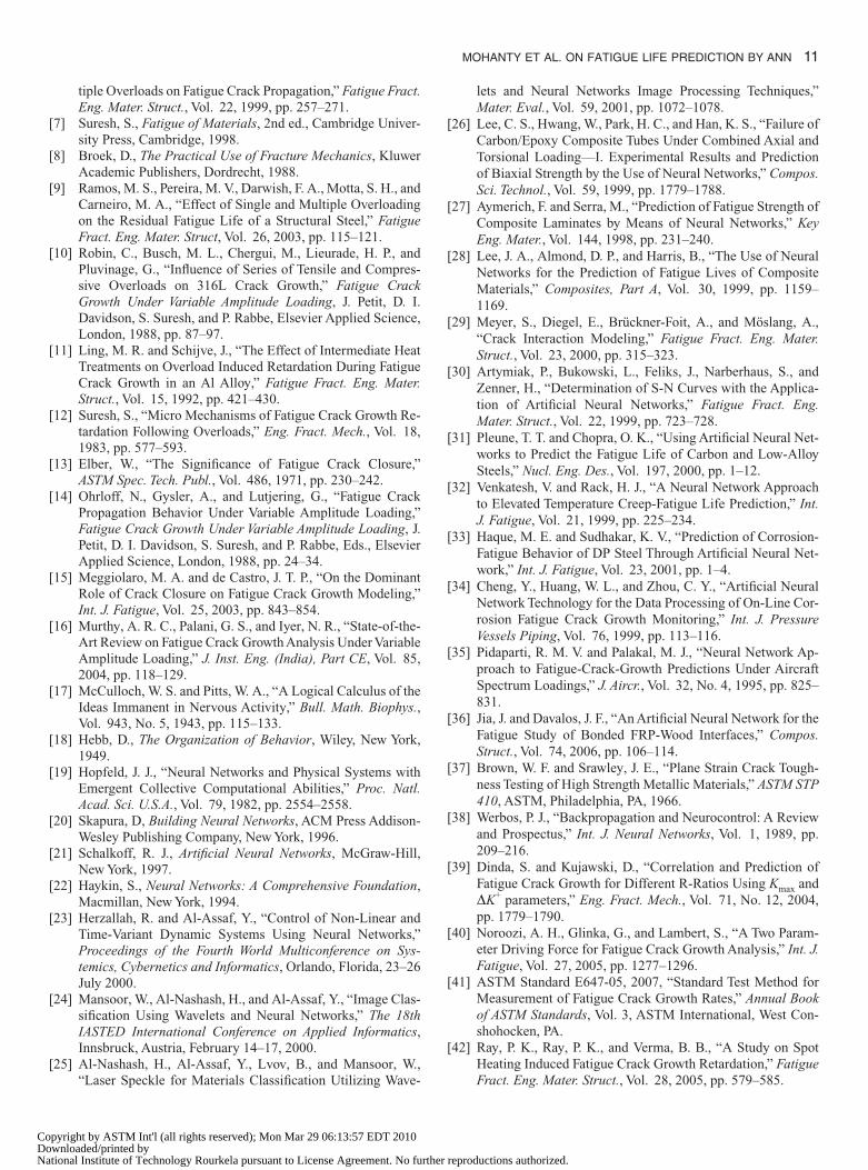
the training database could be enhanced by more experimentaldata. The use of other types of neural networks such as recurrent,associative memory, and self-organizing networks could also im-prove the prediction accuracy.

Acknowledgments

The writers wish to thank CSIR, India, for sponsoring this project(Project No. 22(373)/04/EMR II). The writers also thank Hindalco,Renukoot, India, for supplying the aluminium alloy for this re-search project.

References

TABLE 5—Comparison of ANN and Whe

Materialad

A

(mm)ad

W

(mm)ad

E

(mm) % Error in adA % Error in ad

WNd

A

(K cy)Nd

W

(K c

7020-T7 1.998 2.200 2.134 −6.373 +3.093 32.673 29.80

2024-T3 1.990 2.450 2.181 −8.757 +12.333 40.716 34.51

2.30E-05

4.30E-05

6.30E-05

8.30E-05

1.03E-04

1.23E-04

1.43E-04

1.63E-04

1.83E-04

10.4 10.9

Stress inte

Cra

ck

gro

wth

rate

(da/d

N),

mm

/cycle

Wheeler

ANN

Experimental

overload

point

FIG. 18—Comparison of Wheeler, predic

1.20E-05

3.20E-05

5.20E-05

7.20E-05

9.20E-05

1.12E-04

1.32E-04

1.52E-04

1.72E-04

1.92E-04

10.1 10.6

Stress intens

Cra

ck

gro

wth

rate

(da/d

N),

mm

/cycle

Wheeler

ANN

Experimental

overload

point

FIG. 19—Comparison of Wheeler, predic

[1] Sih, G. C. and Moyer, E. T., “Path Depended Nature of Fa-

pyright by ASTM Int'l (all rights reserved); Mon Mar 29 06:13:57 EDT 2010wnloaded/printed bytional Institute of Technology Rourkela pursuant to License Agreement. No further

tigue Crack Growth,” Eng. Fract. Mech., Vol. 17, 1983, pp.269–280.

[2] Paris, P. C., Tada, H., and Donald, J. K., “Service Load FatigueDamage—A Historical Perspective,” Int. J. Fatigue, Vol. 21,1999, pp. 35–46.

[3] Skorupa, M., “Load Interaction Effects During Fatigue CrackGrowth Under Variable Amplitude Loading—A LiteratureReview, Part 1: Empirical Trends,” Fatigue Fract. Eng. Mater.Struct., Vol. 21, 1998, pp. 987–1006.

[4] Skorupa, M., “Load Interaction Effects During Fatigue CrackGrowth Under Variable Amplitude Loading—A LiteratureReview, Part 2: Qualitative Interpretation,” Fatigue Fract.Eng. Mater. Struct., Vol. 22, 1999, pp. 905–926.

[5] Sadananda, K., Vasudevan, A. K., Holtz, R. L., and Lee, E. U.,“Analysis of Overload Effects and Related Phenomena,” Int.J. Fatigue, Vol. 21, 1999, pp. 233–246.

odel results with experimental data.

NdE

K cy) % Error in NdA % Error in Nd

WNf

A

(K cy)Nf

E

(K cy) % Error in NfA

0.509 +7.093 −2.317 83.721 80.815 +3.596

7.599 +8.290 −8.194 139.384 136.804 +1.886

11.4 11.9 12.4

factor(del.K),MPa.m 1̂/2

NN), and experimental CGR (7020-T7).

.1 11.6 12.1

tor range(del.K),MPa.m 1̂/2

NN), and experimental CGR (2024-T3).

eler m

y) (

2 3

8 3

nsity

11

ity fac

ted (A

[6] Lang, M. and Marci, G., “The Influence of Single and Mul-

reproductions authorized.

MOHANTY ET AL. ON FATIGUE LIFE PREDICTION BY ANN 11

CoDoNa

tiple Overloads on Fatigue Crack Propagation,” Fatigue Fract.Eng. Mater. Struct., Vol. 22, 1999, pp. 257–271.

[7] Suresh, S., Fatigue of Materials, 2nd ed., Cambridge Univer-sity Press, Cambridge, 1998.

[8] Broek, D., The Practical Use of Fracture Mechanics, KluwerAcademic Publishers, Dordrecht, 1988.

[9] Ramos, M. S., Pereira, M. V., Darwish, F. A., Motta, S. H., andCarneiro, M. A., “Effect of Single and Multiple Overloadingon the Residual Fatigue Life of a Structural Steel,” FatigueFract. Eng. Mater. Struct, Vol. 26, 2003, pp. 115–121.

[10] Robin, C., Busch, M. L., Chergui, M., Lieurade, H. P., andPluvinage, G., “Influence of Series of Tensile and Compres-sive Overloads on 316L Crack Growth,” Fatigue CrackGrowth Under Variable Amplitude Loading, J. Petit, D. I.Davidson, S. Suresh, and P. Rabbe, Elsevier Applied Science,London, 1988, pp. 87–97.

[11] Ling, M. R. and Schijve, J., “The Effect of Intermediate HeatTreatments on Overload Induced Retardation During FatigueCrack Growth in an Al Alloy,” Fatigue Fract. Eng. Mater.Struct., Vol. 15, 1992, pp. 421–430.

[12] Suresh, S., “Micro Mechanisms of Fatigue Crack Growth Re-tardation Following Overloads,” Eng. Fract. Mech., Vol. 18,1983, pp. 577–593.

[13] Elber, W., “The Significance of Fatigue Crack Closure,”ASTM Spec. Tech. Publ., Vol. 486, 1971, pp. 230–242.

[14] Ohrloff, N., Gysler, A., and Lutjering, G., “Fatigue CrackPropagation Behavior Under Variable Amplitude Loading,”Fatigue Crack Growth Under Variable Amplitude Loading, J.Petit, D. I. Davidson, S. Suresh, and P. Rabbe, Eds., ElsevierApplied Science, London, 1988, pp. 24–34.

[15] Meggiolaro, M. A. and de Castro, J. T. P., “On the DominantRole of Crack Closure on Fatigue Crack Growth Modeling,”Int. J. Fatigue, Vol. 25, 2003, pp. 843–854.

[16] Murthy, A. R. C., Palani, G. S., and Iyer, N. R., “State-of-the-Art Review on Fatigue Crack Growth Analysis Under VariableAmplitude Loading,” J. Inst. Eng. (India), Part CE, Vol. 85,2004, pp. 118–129.

[17] McCulloch, W. S. and Pitts, W. A., “A Logical Calculus of theIdeas Immanent in Nervous Activity,” Bull. Math. Biophys.,Vol. 943, No. 5, 1943, pp. 115–133.

[18] Hebb, D., The Organization of Behavior, Wiley, New York,1949.

[19] Hopfeld, J. J., “Neural Networks and Physical Systems withEmergent Collective Computational Abilities,” Proc. Natl.Acad. Sci. U.S.A., Vol. 79, 1982, pp. 2554–2558.

[20] Skapura, D, Building Neural Networks, ACM Press Addison-Wesley Publishing Company, New York, 1996.

[21] Schalkoff, R. J., Artificial Neural Networks, McGraw-Hill,New York, 1997.

[22] Haykin, S., Neural Networks: A Comprehensive Foundation,Macmillan, New York, 1994.

[23] Herzallah, R. and Al-Assaf, Y., “Control of Non-Linear andTime-Variant Dynamic Systems Using Neural Networks,”Proceedings of the Fourth World Multiconference on Sys-temics, Cybernetics and Informatics, Orlando, Florida, 23–26July 2000.

[24] Mansoor, W., Al-Nashash, H., and Al-Assaf, Y., “Image Clas-sification Using Wavelets and Neural Networks,” The 18thIASTED International Conference on Applied Informatics,Innsbruck, Austria, February 14–17, 2000.

[25] Al-Nashash, H., Al-Assaf, Y., Lvov, B., and Mansoor, W.,

“Laser Speckle for Materials Classification Utilizing Wave-

pyright by ASTM Int'l (all rights reserved); Mon Mar 29 06:13:57 EDT 2010wnloaded/printed bytional Institute of Technology Rourkela pursuant to License Agreement. No further

lets and Neural Networks Image Processing Techniques,”Mater. Eval., Vol. 59, 2001, pp. 1072–1078.

[26] Lee, C. S., Hwang, W., Park, H. C., and Han, K. S., “Failure ofCarbon/Epoxy Composite Tubes Under Combined Axial andTorsional Loading––I. Experimental Results and Predictionof Biaxial Strength by the Use of Neural Networks,” Compos.Sci. Technol., Vol. 59, 1999, pp. 1779–1788.

[27] Aymerich, F. and Serra, M., “Prediction of Fatigue Strength ofComposite Laminates by Means of Neural Networks,” KeyEng. Mater., Vol. 144, 1998, pp. 231–240.

[28] Lee, J. A., Almond, D. P., and Harris, B., “The Use of NeuralNetworks for the Prediction of Fatigue Lives of CompositeMaterials,” Composites, Part A, Vol. 30, 1999, pp. 1159–1169.

[29] Meyer, S., Diegel, E., Brückner-Foit, A., and Möslang, A.,“Crack Interaction Modeling,” Fatigue Fract. Eng. Mater.Struct., Vol. 23, 2000, pp. 315–323.

[30] Artymiak, P., Bukowski, L., Feliks, J., Narberhaus, S., andZenner, H., “Determination of S-N Curves with the Applica-tion of Artificial Neural Networks,” Fatigue Fract. Eng.Mater. Struct., Vol. 22, 1999, pp. 723–728.

[31] Pleune, T. T. and Chopra, O. K., “Using Artificial Neural Net-works to Predict the Fatigue Life of Carbon and Low-AlloySteels,” Nucl. Eng. Des., Vol. 197, 2000, pp. 1–12.

[32] Venkatesh, V. and Rack, H. J., “A Neural Network Approachto Elevated Temperature Creep-Fatigue Life Prediction,” Int.J. Fatigue, Vol. 21, 1999, pp. 225–234.

[33] Haque, M. E. and Sudhakar, K. V., “Prediction of Corrosion-Fatigue Behavior of DP Steel Through Artificial Neural Net-work,” Int. J. Fatigue, Vol. 23, 2001, pp. 1–4.

[34] Cheng, Y., Huang, W. L., and Zhou, C. Y., “Artificial NeuralNetwork Technology for the Data Processing of On-Line Cor-rosion Fatigue Crack Growth Monitoring,” Int. J. PressureVessels Piping, Vol. 76, 1999, pp. 113–116.

[35] Pidaparti, R. M. V. and Palakal, M. J., “Neural Network Ap-proach to Fatigue-Crack-Growth Predictions Under AircraftSpectrum Loadings,” J. Aircr., Vol. 32, No. 4, 1995, pp. 825–831.

[36] Jia, J. and Davalos, J. F., “An Artificial Neural Network for theFatigue Study of Bonded FRP-Wood Interfaces,” Compos.Struct., Vol. 74, 2006, pp. 106–114.

[37] Brown, W. F. and Srawley, J. E., “Plane Strain Crack Tough-ness Testing of High Strength Metallic Materials,” ASTM STP410, ASTM, Philadelphia, PA, 1966.

[38] Werbos, P. J., “Backpropagation and Neurocontrol: A Reviewand Prospectus,” Int. J. Neural Networks, Vol. 1, 1989, pp.209–216.

[39] Dinda, S. and Kujawski, D., “Correlation and Prediction ofFatigue Crack Growth for Different R-Ratios Using Kmax and∆K+ parameters,” Eng. Fract. Mech., Vol. 71, No. 12, 2004,pp. 1779–1790.

[40] Noroozi, A. H., Glinka, G., and Lambert, S., “A Two Param-eter Driving Force for Fatigue Crack Growth Analysis,” Int. J.Fatigue, Vol. 27, 2005, pp. 1277–1296.

[41] ASTM Standard E647-05, 2007, “Standard Test Method forMeasurement of Fatigue Crack Growth Rates,” Annual Bookof ASTM Standards, Vol. 3, ASTM International, West Con-shohocken, PA.

[42] Ray, P. K., Ray, P. K., and Verma, B. B., “A Study on SpotHeating Induced Fatigue Crack Growth Retardation,” Fatigue

Fract. Eng. Mater. Struct., Vol. 28, 2005, pp. 579–585.

reproductions authorized.