Analysis and simulation of a delay-based service

differentiation algorithm for IPACT-based PONs

November 28, 2011

Abstract

In Passive Optical Networks (PONs) employing the Interleaved Pollingwith Adaptive Cycle Time (IPACT), the literature has focused on provid-ing bandwidth-based service differentiation strategies. This work showshow to provide different levels of delay-based differentiation, and providesa model to characterise the proportional differentiation achieved, which isfurther validated with extensive simulations. Furthermore, we show thatthe delay variance of our algorithm is smaller with respect to conventionalIPACT, with the subsequent jitter reduction for high-priority traffic; andwe further present a mechanism to limit the maximum delay experiencedby high-priority traffic.

Keywords: Passive Optical Networks (PONs); Dynamic Bandwidth As-signment (DBA); Quality of Service (QoS); Delay-based proportional servicedifferentiation.

1 Introduction and related work

Passive Optical Networks (PONs) have been proposed in the literature to over-come the bandwidth bottleneck of xDSL technologies at the network access [1, 2].PONs offer the well-known advantages of optical communications (i.e. highbandwidth capacity, low attenuation and immunity to electromagnetic interfer-ence) together with the benefits of a passive point-to-multipoint architecture(i.e. reduced OAM and no need for power supply).

The typical PON architecture follows a tree topology where the leaf nodesor Optical Network Units (ONUs) are connected to the root node, referred toas the Optical Line Terminal (OLT) via a passive splitter/combiner. In thedownstream direction, the splitter forwards a copy of the incoming signal toall ONUs whereas, in the upstream wavelength, the splitter/combiner combinesthe signals generated by the ONUs into a single one towards the OLT.

Thus, the PON operates as a broadcast-and-select network in the down-stream direction, since the data sourced at the OLT is replicated by the passivesplitter/combiner and delivered at all ONUs. On the other hand, the upstreamwavelength is shared by all ONUs, so a channel access arbitration mechanism

1

must be defined to avoid collisions at the passive splitter/combiner. The Mul-tiPoint Control Protocol for Ethernet PONs (MPCP described in the IEEE802.3ah standard) specifies a mechanism where, the OLT first estimates thedifferent RTTs (Round Trip Times) to the ONUs and secondly, it schedulestransmission windows to the ONUs based on their bandwidth requirements.

A number of Dynamic Bandwidth Allocation (DBA) algorithms for timeslotscheduling have already been proposed in the literature [3], being the InterleavedPolling with Adaptive Cycle Time (IPACT) algorithm [4] the most popular one.Essentially, the OLT and the ONUs coordinate themselves via the exchange oftwo control messages: Report and Gate. The Reports are generated by theONUs to inform the OLT about the bandwidth they need for the next windowscheduling round. With this information, the OLT decides the window size andthe starting transmission time for each ONU. Then, a Gate message with thisinformation is sent to all ONUs.

Concerning Quality-of-Service (QoS) support in PONs, most previous stud-ies have focused on service differentiation based on bandwidth, rather than ondelay. A good summary can be found in [3]. For instance, the authors in [5] pro-pose an algorithm that divides the total upstream bandwidth into fixed-sizedbandwidth units (say 10 Mbps per bandwidth unit), such that, high-priorityONUs receive more bandwidth units than best-effort ones. Further refinementsare proposed in [6, 7, 8] where the ONUs have several Virtual Output Queues(VOQs) for different traffic classes, such that the granted transmission windowis shared by the ONU’s traffic classes following some weighted algorithm thatassigns more time to high-priority VOQs than to low priority ones. Essentially,in most cases, it is the OLT which guarantees a fair sharing of bandwidth be-tween the ONUs, while each ONU partitions the granted transmission windowto the traffic classes following some weighted algorithm [9].

In conclusion, most QoS DBA proposals for PONs have focused on service-differentiation based on bandwidth sharing between traffic classes. Only a fewstudies have taken into account the average delay and jitter of packets froma given ONU, see for instance the studies of the authors in [10, 11, 12, 13].However, these studies do not provide a clear delay-based proportional differ-entiation algorithm, an important feature for a number of applications such ashighly interactive networked gaming or IP telephony.

Thus, this work proposes a new delay-based service differentiation DBA algo-rithm for IPACT-based PONs and its analysis and simulation-based validation.This new algorithm forces the transmission of high-priority traffic more oftenthan low-priority one such that the expected average cycle time for high-prioritypackets is much smaller (and also proportional and configurable) than for low-priority ones. Its analysis and performance evaluation is further conducted andproved with extensive simulation-based experiments.

The reminder of this work is thus organised as follows: Section 2 reviewsprevious work concerning the delay analysis of IPACT as following [14, 15], butwithout any service differentiation. Section 3 extends this model to includedelay-based service differentiation, and Section 4 further analyses the case ofexcessive traffic load, and how the algorithm guarantees the delay experienced

2

by the high-priority packets below an upper bound, even at the expense of low-priority traffic loss. Section 5 provides a number of experiments to validatethe equations derived through the analytical sections and to illustrate and com-pare the benefits of our algorithm with respect to conventional IPACT. Finally,Section 6 concludes this work with a summary of the main contributions andconclusions.

2 Analytical review of the classic gated PON

TDM model

This section reviews the delay and bandwidth analysis of IPACT, as studied bythe authors in [15] Section 3B. The reader is referred to this work for furtherdetails.

2.1 Assumptions

In IPACT, the OLT assigns transmission windows (via the Grant message) to theONUs based on their bandwidth requests and some internal rules to guaranteea fair share of the total bandwidth.

To simplify the analysis, we assume the following conditions:

• We study IPACT steady-state behaviour.

• The N ONUs are d km distant from the OLT.

• The ONUs offer a fixed traffic load over time ρi, i = 1, . . . , N . Further-more, the i-th ONU receives traffic from its users following a Poisson pro-cess with rate λi packets/sec. Also, each packet requires a fixed amountof service time E[X ] = 1

µcomputed as:

E[X ] =1

µ=

8B

Csecs (1)

where B refers to the packet size and C denotes the line rate. ForB = 1518bytes and C = 1 Gbps, the service time required is E[X ] = 12.14µs perpacket.

Hence, the i-th ONU offers ρi, i = 1, . . . , N traffic load as:

ρi =λi

µ(2)

Finally, the total offered load ρT , that is, the sum of all individual trafficloads ρi must be smaller than unity:

ρT =

N∑

i=1

ρi < 1 (3)

3

V1(0) V2(0) V3(0) V1(1) V2(1) V3(1)

T1(0)

T2(0)

T3(0)

P1 P2 P3 P4 P5

Figure 1: Definitions for a PON with N = 3

2.2 Analysis of the Average Cycle Time

Now, consider the example of a PON with N = 3 ONUs whose transmissionwindows are granted as shown in Fig. 1. Let Ti(k) refer to the k-th cycle time forthe i-th ONU, and let Vi(k) denote the transmission window of user i at discretetime k, where k = 0, 1, . . . (the squares in the figure). Clearly, the transmissionwindows have a variable length which depend on the number of packet arrivalsduring its previous cycle time. For instance, at time k = 1, the size of V1(1)in the figure depends on the number of packet arrivals, say N1(1), during itsprevious cycle time T1(0), in this case, five packets (P1 to P5 in the figure).Under the assumption that packet arrivals follow a Poisson process with rateλi, the probability to have exactly n packet arrivals within its previous cycletime of length Ti(k) secs follows the Poisson probability density function:

P (Ni(k + 1) = n) =(λiTi(k))

n

n!e−λiTi(k), i = 0, 1, . . . (4)

where the average number of packet arrivals is:

E[Ni(k + 1)] = λiE[Ti(k)] packets (5)

where E[Ti(k)] is the mean cycle time for user i at time k. Thus, under theassumption that each packet requires an average amount of service time of S = 1

µ

secs, then the average transmission window required by the i-th ONU at timek + 1 is:

E[Vi(k + 1)] =1

µE[Ni(k + 1)] = ρiE[Ti(k)] secs (6)

Finally, the average cycle time E[Ti(k)] is computed as the sum of the pre-vious N windows plus the guard and report times, which are represented by thegaps in the figure:

E[Ti(k)] =

N∑

i=1

E[Vi(k)] +N(Tguard + Treport) secs (7)

where Tguard is the guard time between windows (1.5µs recommended at 1Gbps) and Treport =

8·64109 ≈ 0.5µs is the transmission time of a 64-byte Report

message [15].

4

In the steady-state, it can be observed by simulation that the system shows astable average cycle time E[T ] which does not depend on time k. Similarly, thetransmission windows Vi(k) also show a very stable average size E[Vi]. Hence:

E[Vi] = ρiE[T ], i = 1, . . . , N (8)

E[T ] =N∑

i=1

ρiE[T ] +NT0 (9)

where T0 = Tguard + Treport for brevity.Solving the above for E[T ] yields:

E[T ] =NT0

1−∑

i ρi=

NT0

1− ρT(10)

Thus, E[T ] only depends on the total load ρT , the number N of ONUs, and theguard and Report times T0 = Tguard + Treport.

Finally, it is worth remarking that Eq. 10 is only valid at medium to highloads (see [15]) as explained next: Essentially, the Gate message cannot departbefore its associated Report packet has arrived at the OLT. To meet this con-dition, it is then required that the average cycle time E[T ] is greater than theRound-Trip Time (RTT) and processing delay of the Report packet Tproc. Inother words, Eq. 10 is valid only when:

E[T ] =NT0

1− ρT> RTT + Tproc (11)

which sets a minimum load value for Eq. 10 to be valid of:

ρT > 1−NT0

RTT + Tproc

(12)

Typically, for a 1 Gbps PON with N = 32 ONUs, d = 10 km distancebetween the OLT and ONUs and assuming a value of Tproc = 35µs, the aboverequirement is:

ρT > 0.24

In the cases where this condition cannot be met, the cycle time is imposedby RTT and the processing time of a report packet. For the example above:

Tmin = RTT + Tproc = 210km

2 · 105km/s+ 35µs = 135µs

2.3 Maximum delay analysis

The delay experienced by a random packet arrival lies between E[T ] and 2E[T ].The former arises when the packet arrives exactly before the transmission ofthe Report message to the OLT, and assuming an empty queue, whereas the

5

second occurs when the packet arrives just after the Report message has beensent to the OLT, as noted in [15]. Hence, the average delay experienced by agiven packet is proportional to the average cycle time E[T ]. We will use E[T ] asthe performance metric to evaluate our DBA algorithm, bearing in mind thatthe average delay experienced by a packet is proportional to E[T ].

3 Analysis of the Gated PON TDM model with

delay differentiation

3.1 Scheduling algorithm with delay differentiation

Now, consider that each ONU employs two output queues, one per traffic class:High and Low Priority (HP and LP). The former traffic class is expected to con-tain packets from delay-sensitive applications, typically video streaming, voiceover IP, or online gaming, whereas the second one is for best-effort applications.

The goal is to design a transmission scheduling algorithm that favors HPover LP traffic in terms of delay experienced at the ONU. Most previous studieshave proposed to schedule the HP traffic ahead of the transmission window inorder to save delay. Our algorithm differs from such studies since it proposes toseparate HP and LP traffic Reports such that, HP traffic is sent to the OLT moreregularly than LP traffic. This is expected to minimise the delay experiencedby high-priority packet arrivals at the ONUs, however at the expense of a delayincrease for the LP traffic. An example of operation for three ONUs is shownin Fig. 2.

1 31 31 1 22 2 2 3 3

Thp(1)

321 1

Tlp(1)

Thp(2)

Thp(3)

Figure 2: Algorithm with delay differentiation. Case M = 1.

In this example, HP traffic (shadowed boxes) from the three ONUs are sentto the OLT more regularly than LP traffic (white boxes). We observe two typesof cycle times, one for HP traffic T (HP ) and another one for LP traffic T (LP ),where T (HP ) ≤ T (LP ). Basically, the OLT polls the HP packets for the threeONUs and the LP traffic for a single ONU (ONU 1 in the example) in one HPcycle. On the second round, the OLT polls the HP packets for the three ONUsagain, and the LP traffic from the second ONU. Finally, on the third round, theOLT polls the HP traffic from the three ONUs and the LP traffic for the thirdONU, thus completing an LP cycle. In the fourth round, the OLT polls the HPtraffic from the three ONUs and the LP traffic from the first ONU, just like in

6

the first round. Hence, in this case, the LP cycle is as large as three HP cycles,as shown in Fig. 2.

Typically, the HP transmission windows are smaller than the LP ones fortwo reasons: First, delay-sensitive applications generate less traffic than best-effort applications. Secondly, the HP VOQ is polled more regularly than theLP VOQ, thus the latter one aggregates more packets on every LP cycle.

As a generalisation, let M refer to the number of LP ONUs polled withinthe HP polling cycle. Fig. 3.1 shows the cases for M = 1, 2, 3. As shown,case M = 3 produces the same cycle time for HP and LP traffic, therefore nodelay-based service differentiation is performed.

1 31 1 1 22 2 3 3 321 1

TLP

THP

2

THP THP

TLP

3

(a) M = 1, N = 3

1 31 12 2 3 3 321 121 1 3 2 2 2

TLP

THP THP

TLP

THPTHP

TLP

(b) M = 2, N = 3

1 1 12 2 3 3 321 13 3 1 2 2 2 3

TLP

THP THP

TLP TLP

THP

(c) M = 3, N = 3

Figure 3: Algorithm with delay differentiation. Cases M = 1, 2 and 3. Timingindicated for ONU 1

Next section analyses the average cycle time per traffic class.

3.2 Analysis

Following the same reasoning as section 2, the average HP transmission windowsrequested by the ONUs depend on the average amount of traffic aggregated ontheir previous cycle time. Clearly, the average HP traffic aggregated on a cycle

is much smaller than for LP traffic, since the cycle time is smaller. Let E[V(HP )i ]

and E[V(LP )i ] refer to the average transmission windows requested by the i-th

ONU for HP and LP traffic respectively. Following eq. 8, in the steady-state,the transmission windows for HP and LP traffic are:

E[V(HP )i ] = ρ

(HP )i E[T (HP )] (13)

E[V(LP )i ] = ρ

(LP )i E[T (LP )] (14)

where ρ(HP )i = phρi and ρ

(LP )i = (1− ph)ρi for some ph ∈ (0, 1). Here ph refers

to the percentage of HP traffic over the total. Again, the total traffic must besmaller than unity:

ρT =

N∑

i=1

(

ρ(HP )i + ρ

(LP )i

)

< 1 (15)

7

Now, let E[T (HP )] and E[T (LP )] refer to the average HP and LP cycle timesrespectively. Remark from Fig. 3.1 that the average HP cycle time accounts forthe N HP transmission windows plus another M LP windows plus the N guardand Report times, denoted by T0. Hence:

E[T (HP )] =

N∑

i=1

E[V(HP )i ] +

M∑

i=1

E[V(LP )i ] +NT0 (16)

which further yields:

E[T (HP )] = NρiE[T (HP )] +Mρi(1 − ph)E[T (LP )] +NT0 (17)

since:

E[V(HP )i ] = ρiphpE[T (HP )] (18)

E[V(LP )i ] = ρi(1− php)E[T (LP )] (19)

from eq. 13Similarly, for E[T (LP )], we have that:

M ·E[T (LP )] = N

N∑

i=1

E[V(HP )i ] +N

M∑

i=1

E[V(LP )i ] +N2T0 (20)

since N average HP cycle times comprise M average LP cycle times, as shownfrom Fig. 3.1. Thus:

E[T (LP )] =N

M

N∑

i=1

E[V(HP )i ] +

N

M

M∑

i=1

E[V(LP )i ] +

N2

MT0 (21)

Therefore, we can use eqs. 17 and 21 as a system with two equations andtwo unknowns to solve for E[T (HP )] and E[T (LP )]:

E[T (HP )] =NT0

1− ρ(22)

E[T (LP )] =N

M

NT0

1− ρ(23)

Concludingly, it can be observed that there is an M/N relationship betweenthe HP and LP average cycle times, as shown from:

E[T (HP )]

E[T (LP )]=

M

N(24)

This relationship allows the scheduler to define the level of delay-based dif-ferentiation between HP and LP traffic, just by adjusting the appropriate valueof M in the scheduler. The case M = 1 refers to maximum delay differencebetween HP and LP traffic, whereas the M = N case refers to no differencebetween HP and LP traffic.

8

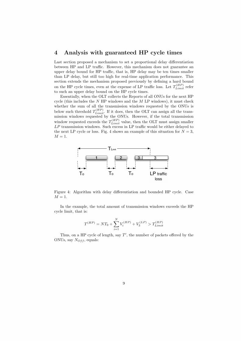
4 Analysis with guaranteed HP cycle times

Last section proposed a mechanism to set a proportional delay differentiationbetween HP and LP traffic. However, this mechanism does not guarantee anupper delay bound for HP traffic, that is, HP delay may be ten times smallerthan LP delay, but still too high for real-time application performance. Thissection extends the mechanism proposed previously by defining a hard bound

on the HP cycle times, even at the expense of LP traffic loss. Let T(HP )Limit refer

to such an upper delay bound on the HP cycle times.Essentially, when the OLT collects the Reports of all ONUs for the next HP

cycle (this includes the N HP windows and the M LP windows), it must checkwhether the sum of all the transmission windows requested by the ONUs is

below such threshold T(HP )Limit. If it does, then the OLT can assign all the trans-

mission windows requested by the ONUs. However, if the total transmission

window requested exceeds the T(HP )Limit value, then the OLT must assign smaller

LP transmission windows. Such excess in LP traffic would be either delayed tothe next LP cycle or loss. Fig. 4 shows an example of this situation for N = 3,M = 1.

1 2 3 3

TLimit

To LP traffic

loss

ToTo

Figure 4: Algorithm with delay differentiation and bounded HP cycle. CaseM = 1.

In the example, the total amount of transmission windows exceeds the HPcycle limit, that is:

T (HP ) = NT0 +

N∑

i=1

V(HP )i + V

(LP )3 > T

(HP )Limit

Thus, on a HP cycle of length, say T ′, the number of packets offered by theONUs, say NOff , equals:

9

E[NOff.] =

(

N∑

i=1

λiphp

)

T ′

+ M1

N

(

N∑

i=1

λi(1− php)

)

N

MT ′

=ρphpT

′

E[X ]+

ρ(1− php)T′

E[X ]

=ρT ′

E[X ]packets (25)

which accounts for the HP and the LP packets offered on cycle of length T ′.

The total number of packets NLimit allowed in a T(HP )Limit requires to substract

the N guard and report times and divide by the average packet service timeE[X ]. In other words:

NLimit =T

(HP )Limit −NT0

E[X ]packets (26)

Finally, the percentage of LP packet loss equals:

PLoss =E[NOff ]−NLimit

E[NOff.]

=ρTLimit

E[X] −TLimit−NT0

E[X]

TLimit−NT0

E[X]

=TLimit(ρ− 1) +NT0

ρTLimit

(27)

5 Experiments

This section shows a number of experiments to demonstrate the equations andconclusions obtained in the previous sections in a number of realistic situations.

5.1 Validation of the average cycle times E[T ], E[T (HP )]and E[T (LP )]

In this first experiment, the goal is to validate the equations obtained previ-ously for E[T (HP )] and E[T (LP )] (eqs. 17 and 21) in the delay-based servicedifferentiation algorithm for IPACT-based PONs.

The experiments in both cases consider the following system parameters:

• Line rate: C = 1 Gbps.

10

• Guard time: Tguard = 1.5µs

• Processing time of a Report packet: Treport = 0.512µs

• Percentage of HP traffic over the total: ph = 0.4

Figs. 5(a)-5(d) show the E[T (HP )] and E[T (LP )] for 32 ONUs and differentvalues of M in the scheduler. As shown, for M = 1, the delay differentiationis maximum (1/32 ratio), and for M = 32 there is no delay differentiation.Intermediate values of M = 4 and M = 16 are also shown. Additionally, it canbe shown that the equations accurately match with the simulation experiments,thus validating the analytical sections.

0.1 0.2 0.3 0.4 0.5 0.6 0.7 0.8 0.90

2

4

6

8

10

12

14

16

18

20

Load ρT

E[ T

](m

s)

E[ TLP] sim

E[ TLP theo]

E[ THP] sim

E[ THP] theo

(a) M/N = 1/32

0.1 0.2 0.3 0.4 0.5 0.6 0.7 0.8 0.90

0.5

1

1.5

2

2.5

3

3.5

4

4.5

5

Load ρT

E[ T

](m

s)

E[ TLP] sim

E[ TLP theo]

E[ THP] sim

E[ THP] theo

(b) M/N = 4/32

0.1 0.2 0.3 0.4 0.5 0.6 0.7 0.8 0.90

0.2

0.4

0.6

0.8

1

1.2

Load ρT

E[ T

](m

s)

E[ TLP] sim

E[ TLP theo]

E[ THP] sim

E[ THP] theo

(c) M/N = 16/32

0.1 0.2 0.3 0.4 0.5 0.6 0.7 0.8 0.90

0.1

0.2

0.3

0.4

0.5

0.6

Load ρT

E[ T

](m

s)

E[ TLP] sim

E[ TLP theo]

E[ THP] sim

E[ THP] theo

(d) M/N = 32/32

Figure 5: Average cycle times E[T (HP )] and E[T (LP )] for different M/N ratios:(a) M

N= 1

32 , (b)MN

= 432 , (c)

MN

= 1632 , (d)

MN

= 3232

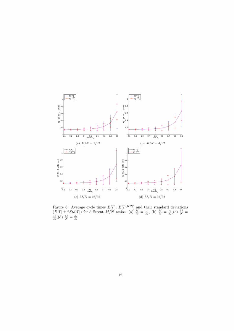
Figs. 6(a)-6(d) show the average cycle time plus/minus twice its standarddeviation for E[T ] and E[T (HP )]. As shown, although the average cycle timeare the same in both cases, the standard deviation is smaller in our algorithm,thus producing less spread HP cycle times, which favors for a small jitter fordelay-sensitive applications, especially at high loads and for low values of M .The average cycle times and their standard deviation have been estimated fromsimulation.

11

0.1 0.2 0.3 0.4 0.5 0.6 0.7 0.8 0.90

0.2

0.4

0.6

0.8

1

Load ρT

E[ T

] ±

2 σ

(T)

(m

s)

E[ T ]

E[ THP]

(a) M/N = 1/32

0.1 0.2 0.3 0.4 0.5 0.6 0.7 0.8 0.90

0.2

0.4

0.6

0.8

1

Load ρT

E[ T

] ±

2 σ

(T)

(m

s)

E[ T ]

E[ THP]

(b) M/N = 4/32

0.1 0.2 0.3 0.4 0.5 0.6 0.7 0.8 0.90

0.2

0.4

0.6

0.8

1

Load ρT

E[ T

] ±

2 σ

(T)

(m

s)

E[ T ]

E[ THP]

(c) M/N = 16/32

0.1 0.2 0.3 0.4 0.5 0.6 0.7 0.8 0.90

0.2

0.4

0.6

0.8

1

Load ρT

E[ T

] ±

2 σ

(T)

(m

s)

E[ T ]

E[ THP]

(d) M/N = 32/32

Figure 6: Average cycle times E[T ], E[T (HP )] and their standard deviations(E[T ]± 2Std[T ]) for different M/N ratios: (a) M

N= 1

32 , (b)MN

= 432 ,(c)

MN

=1632 ,(d)

MN

= 3232

12

5.2 Experiments under heavy traffic conditions

Figs. 7(a)-7(d) show the behaviour of the delay-based service differentiationDBA algorithm proposed in this article under heavy-traffic conditions, thatmeans, for total loads in the range 1 ≤ ρT ≤ 2. Two delay limits are considered

in the experiments: T(HP )Limit = 3.2ms (top) and T

(HP )Limit = 8ms (bottom). As

shown, the values of the HP traffic cycles are kept below the T(HP )Limit bound, in

both cases while the LP traffic cycles are much higher. In addition, to guaranteesuch bounded delays, LP priority traffic is lost, as explained in Section 4.

0.8 1 1.2 1.4 1.6 1.8 20

20

40

60

80

100

Load ρT

E[ T

] (m

s)

E[ TLP] sim

E[ TLP theo]

E[ THP] sim

E[ THP] theo

(a) TLimit = 3.2ms Average cycle time

0.8 1 1.2 1.4 1.6 1.8 20

10

20

30

40

50

60

70

80

Load ρT

% P

acke

t Los

s

Loss simLoss teoLoss(HP) simLoss(LP) sim

(b) TLimit = 3.2ms Packet Loss

0.8 1 1.2 1.4 1.6 1.8 20

50

100

150

200

250

Load ρT

E[ T

] (m

s)

E[ TLP] sim

E[ TLP theo]

E[ THP] sim

E[ THP] theo

(c) TLimit = 8ms Average cycle time

0.8 1 1.2 1.4 1.6 1.8 20

10

20

30

40

50

60

70

80

Load ρT

% P

acke

t Los

s

Loss simLoss teoLoss(HP) simLoss(LP) sim

(d) TLimit = 8ms Packet Loss

Figure 7: Average cycle times and packet loss ratios for the delay differentiationDBA algorithm under heavy traffic conditions: TLimit = 3.2ms, avg. cycletime (a) and packet loss ratio (b); TLimit = 8ms, avg. cycle time (c) and packetloss ratio (d).

6 Summary and conclusions

This article has proposed a new Dynamic Bandwidth Allocation (DBA) al-gorithm to provide delay-based service differentiation of IPACT-based PONs.Essentially, the algorithm defines two types of polling cycles for the OLT: thehigh- and low-priority (HP and LP) cycles, being the former more regularly per-

13

formed than the latter ones. Thus, on every HP cycle, all ONUs are polled forreporting the transmission windows required for their HP traffic, whereas onlysome of the ONUs are also polled for their LP traffic demands. This strategyclearly favors the creation of short HP cycles and long LP cycles, with a prede-fined ratio between them. This work further provides a model to characterisesuch a ratio, which is further validated with simulation.

This article takes one step further into delay-based service diffentiation bydefining un upper bound on the HP cycle times, which causes LP traffic lossto guarantee the HP traffic delay bound. Such a mechanism is very interest-ing when the HP traffic comprises packets from applications with tight delayrequirements, such as video streaming, IP telephony or online gaming, since itguarantees an upper delay bound.

We finally show a number of experiments that illustrate the meaning of thedifferent parameters of the algorithm and their impact in the whole systemperformance.

Acknowledgements

The authors would like to acknowledge the support to this work by the UC3M-CAM -funded Greencom project (under code CCG10-UC3M-TIC-5624), and bythe FP7-EU funded MyUI project (grant FP7-ICT-248606).

Additionally, part of this work has been funded by the T2C2 Spanish project(under code TIN2008-06739-C04-01).

References

[1] G. Pesavento and M. Kelsey, “PONs for the broadband local loop,” Light-wave, vol. 16, no. 10, pp. 68–74, Sept. 1999.

[2] B. Lung, “PON architecture futureproofs FTTH,” Lightwave, vol. 16,no. 10, pp. 104–107, Sept. 1999.

[3] M. McGarry, M. Maier, and M. Reisslein, “Ethernet PONs: A survey ofdynamic bandwidth allocation (DBA) algorithms,” IEEE CommunicationsMagazine, vol. 42, no. 8, pp. 8 – 15, Aug. 2004.

[4] G. Kramer, B. Mukherjee, and G. Pesavento, “Interleaved polling withadaptive cycle time (IPACT): A dynamic bandwidth distribution schemein an optical access network,” Photonic Network Communications, vol. 4,no. 1, pp. 89–107, 2002.

[5] M. Ma, Y. Zhu, and T. H. Chen, “A bandwidth guaranteed polling MACprotocol for Ethernet Passive Optical Networks,” in Proc. of IEEE INFO-COM, vol. 1, San Francisco, CA, USA, 2003, pp. 22–31.

14

[6] L. Zhang, E.-S. An, C.-H. Youn, H.-G. Yeo, and S. Yang, “Dual DEB-GPS scheduler for delay-constraint applications in Ethernet Passive OpticalNetworks,” IEICE Trans. Communications, vol. E86-B, no. 5, pp. 1575–1584, May 2003.

[7] C. M. Assi, Y. Ye, S. Dixit, and M. A. Ali, “Dynamic bandwidth allocationfor Quality of Service over Ethernet PONs,” IEEE J. Selected Areas inCommunications, vol. 21, no. 9, pp. 1467–1477, Nov. 2003.

[8] S.-I. Choi and J.-D. Huh, “Dynamic bandwidth allocation for multimediaservices over Ethernet PONs,” ETRI Journal, vol. 24, no. 6, pp. 465–468,Dec. 2002.

[9] B. Moon and H. Song, “Hierarchical Ethernet-PON design with QoS sup-porting by eligible reporting,” in Proc. of Asia-Pacific Conf. in Communi-cations, Busan, Aug. 2006, pp. 1–5.

[10] C. Park, D. Han, and B. Kim, “Packet delay analysis of dynamic band-width allocation scheme in an Ethernet PON,” Lecture Notes in ComputerScience, vol. 3420, pp. 161–168, 2005.

[11] C. G. Park, D. H. Han, and K. W. Rim, “Packet delay analysis of symmetricgated polling system for DBA scheme in an EPON,” TelecommunicationSystems, vol. 30, pp. 13–34, 2005.

[12] T. Berisa, Z. Ilic, and A. Bazant, “Absolute delay variation guaranteesin passive optical networks,” IEEE/OSA J. Lightwave Technology, no. 99,2011.

[13] F. An, Y. Hsueh, K. Kim, I. White, and L. Kazovsky, “A new dynamicbandwidth allocation protocol with quality of service in ethernet-basedpassive optical networks,” in Proc. of IASTED Int. Conf. Wireless andOptical Communications (WOC 2003), vol. 3, 2003, pp. 165–169.

[14] S. Bhatia, D. Garbuzov, and R. Bartos, “Analysis of the gated IPACTscheme for EPONs,” in IEEE Proc. of Int. Conf. Communications, vol. 6,2006, pp. 2693–2698.

[15] B. Lannoo, L. Verslegers, D. Colle, M. Pickavet, M. Gagnaire, and P. De-meester, “Analytical model for the IPACT dynamic bandwidth allocationalgorithm for EPONs,” OSA J. Optical Networking, vol. 6, no. 6, pp. 677–688, 2007.

15