The Regional Economics Applications Laboratory (REAL) is a cooperative venture between the University of Illinois and the Federal Reserve Bank of Chicago focusing on the development and use of analytical models for urban and regional economic development. The purpose of the Discussion Papers is to circulate intermediate and final results of this research among readers within and outside REAL. The opinions and conclusions expressed in the papers are those of the authors and do not necessarily represent those of the Federal Reserve Bank of Chicago, Federal Reserve Board of Governors or the University of Illinois. All requests and comments should be directed to Geoffrey J. D. Hewings, Director, Regional Economics Applications Laboratory, 607 South Matthews, Urbana, IL, 61801-3671, phone (217) 333-4740, FAX (217) 244-9339. Web page: www.uiuc.edu/unit/real

AN INVESTIGATION OF INDUSTRY ASSOCIATIONS, ASSOCIATION LOOPS, AND ECONOMIC COMPLEXITY: APPLICATION TO CANADA AND THE UNITED STATES

by

Chokri Dridi and Geoffrey J.D. Hewings

REAL 01-T-14 November, 2001 (Published in 2002: Economic Systems Research 14, 3, 275-296)

1

AN INVESTIGATION OF INDUSTRY ASSOCIATIONS, ASSOCIATION LOOPS,

AND ECONOMIC COMPLEXITY: APPLICATION TO CANADA AND THE UNITED STATES

Chokri Dridi Department of Agriculture and Consumer Economics, and Regional Economics Applications Laboratory (REAL), University of Illinois at Urbana-Champaign cdridi@uiuc.edu Geoffrey J.D. Hewings Regional Economics Applications Laboratory (REAL), University of Illinois at Urbana-Champaign hewings@uiuc.edu

ABSTRACT: Various methods were proposed to understand the linkages in an input-output system; however many focused only on the identification of key sectors in the economy. An alternative approach, identifying analytically importance of elements and combinations of elements was proposed as a field of influence theory (Sonis et al., 1996). The purpose of this paper is to offer a complementary approach to the field of influence and the so-called 'Matrioshka principal' (Sonis and Hewings, 1990); the objectives are to identify simple row-column associations (i.e. statistical dependence), seek hierarchical associations between supply and demand in input-output systems and the decomposition of economic complexity into finite stages. For the identification of simple dependencies between rows and columns, we use a log-linear regression and for hierarchical associations and the identification of complexity stages, we use the data analysis technique known as dual scaling. Results of both approaches will be applied to input-output tables of the US and Canada. Journal of Economic Literature Classification: C12, C20, C67, O51, O57, R15

Keywords: Dual scaling; industry associations; loops; economic complexity 1. INTRODUCTION

In an earlier paper, analysis revealed that while the macro structures (in terms of the

percentage of total production accounted for by each sector) of a set of Midwest US states were

very similar, visual presentations of the input-output structures using the multiplier product

matrix methodology (see Sonis et al., 2000) revealed some sharp differences. While visual

2

differentiation may be a valuable first stage in an examination of structure, some more formal

evaluation is still needed. However, analysts have struggled for years to develop appropriate

measures for documenting differences and similarities between matrix-based structures. Some of

these measures will be reviewed in this paper but there is a sense that none provides the

comprehensive assessment that the visual affords. In this paper, an additional approach will be

considered; while it is not promoted as comprehensive, it does have the distinction of examining

both input and output structure at the same time.

This paper aims to further the investigation into the composition of the economic

structure through the internal associations or statistical dependences between supplying and

demanding sectors. Understanding the internal associations in an input-output system is of major

interest especially in assessing the ripple effect of a fundamental change in the interindustry

supply or demand of a particular commodity. We view this approach as being different from the

field of influence approach (see Sonis and Hewings, 1992) because the latter focuses on the

effect of a change in particular elements of the technical block in an input-output system without

distinguishing whether the change is coming from a change in the demand of inputs

(technological conditions) or in the supply (market conditions). In contrast, the approach we

present in this paper provides a way of mapping out the relative effects of a change in demand or

supply in a sector as a whole. This methodology allows for the establishment of priorities

according to the dependences should rationing need to be implemented. In addition, the slicing

procedure that yields the internal association loops can be used for a crude decomposition of the

complexity of interindustrial flows into few stages, a more elaborate method for understanding

the economic complexity of interindustry flows was offered by Sonis and Hewings (2000).

3

A first assessment of industries associations is achieved by using a log-linear regression

described in Krzanowski (1998), applied to contingency tables. The log-linear regression

identifies cells in the input-output table that show relatively higher row-column dependence.

Further investigation of the interindustries associations is made possible through the

decomposition of the total association into hierarchical loops where the method employed is

derived from the field of data analysis that is known as dual scaling, a term coined by Nishisato

(1980). Dual scaling is considered as a technique of multivariate descriptive analysis; it is not

inferential in the sense that it does not draw conclusions that can be generalized to a larger

population. The method is concerned with the explanation and the extraction of complex

information from a particular data set without suggesting a generalization of the results to other

cases. The dual scaling method is similar to principal components analysis (PCA) for categorical

data approach or ANOVA; however, the existence of a dual solution, as will be seen later, makes

dual scaling different from the well-known PCA and allows for additional insights. For example,

in O'Huallachain (1984), a reassessment of PCA was made where the method was applied to

identify row clusters (R-mode) and column clusters (Q-mode) but the methodology was not used

to assess the relationship between row-sectors and column-sectors. Indeed, in input-output

tables, not only the rows and columns have different roles but they are also related through

demand and supply and the state of the technology.

In the next section, a formal description of the log-linear regression method will be

presented. In section 3, the method of dual scaling will be presented and discussed. In section 4,

the log-linear and dual scaling methods are applied to the US and Canada 1995 input-output

tables to identify coefficients with high associations between supplies and demands in the

4

interindustry matrix and to identify complexity stages. We will conclude with a summary of

results and further research possibilities.

2. LOG-LINEAR MODEL OF CONTINGENCY TABLES

In input-output tables, if we consider that the monetary values are an indicator of the

frequency of exchanges between industries, then the use of the interindustry flows along with the

primary inputs (wages, imports, and gross profits), the final demand (investment, household

consumption, government expenditure, and exports), and the input and output totals constitute a

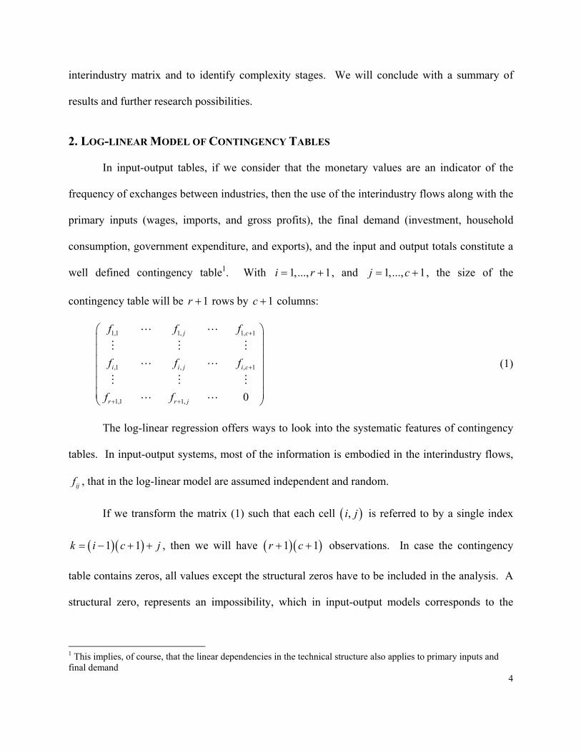
well defined contingency table1. With 1,..., 1i r= + , and 1,..., 1j c= + , the size of the

contingency table will be 1r + rows by 1c + columns:

1,1 1, 1, 1

,1 , , 1

1,1 1,

0

j c

i i j i c

r r j

f f f

f f f

f f

+

+

+ +

(1)

The log-linear regression offers ways to look into the systematic features of contingency

tables. In input-output systems, most of the information is embodied in the interindustry flows,

ijf , that in the log-linear model are assumed independent and random.

If we transform the matrix (1) such that each cell ( ),i j is referred to by a single index

( )( )1 1k i c j= − + + , then we will have ( )( )1 1r c+ + observations. In case the contingency

table contains zeros, all values except the structural zeros have to be included in the analysis. A

structural zero, represents an impossibility, which in input-output models corresponds to the

1 This implies, of course, that the linear dependencies in the technical structure also applies to primary inputs and final demand

5

unique zero in cell ( )1, 1r c+ + , since any other zeros, if they exist, are not structural and they

depend on the economy under study. If we omit the structural zero, the values in the

contingency table can be re-arranged in a column vector [ ]kz=Z of random and independent

variables kz . The dimension of Z is ( )( )1 1 1r c+ + − .

Let M be a dummy variable for the mean of the random variable kz , then it will take the

value 1 for all the cells, therefore M is a unit column vector of dimension ( )( )1 1 1r c+ + − . We

will use 1 ,..., ,...,i rX X X and 1,..., ,...,j cY Y Y as dummy variables to describe the row and

columns effects. The dummy variables are obtained as follows: for a value kz such that

( )( )1 1k i c j= − + + , the kth observation will have the value of 1 in the kth row of the column

vectors iX and jY and the value zero for all the other dummy variables. All the explanatory

variables are column vectors of dimension ( )( )1 1 1r c+ + − and are summarized by:

[ ] [ ]1km= =M ; ( )( )1,..., 1 1 1k r c∀ = + + − (2)

[ ]i kix=X ; 1,...,i r∀ = (3)

j kjy = Y ; 1,...,j c∀ = (4)

The linear model has the following features:

(i) kz , ( )( )1,..., 1 1 1k r c∀ = + + − are independent random variables and have a mean kµ .

(ii) The explanatory variables provide the following linear predictor:

6

1 1

1 1

r c

k k i ki j kji j

r c

i ki j kji j

m x y

x y

η α β γ

α β γ

= =

= =

= + +

= + +

∑ ∑

∑ ∑ (5)

(iii) The relation between (i) and (ii) is that ( )k kg µ η= , where ( ).g is called the link

function of the model, which links kη , the linear predictor to the mean kµ when

independence is assumed.

For contingency tables, where the volume of exchanges and the margins are not fixed the

appropriate distribution would be the independent Poison distribution whose link function is

( ) ( )logk kg µ µ= (Krzanowski, 1998). In case when the model is saturated, the number of

coefficients to be estimated will be equal to the number of observations, i.e. ( )( )1 1 1r c+ + − ,

and the fitted values ˆkµ is equal to kz . If we assume complete independence between rows

and columns, there will be absence of interaction effects between rows and columns and the

log-linear model becomes:

( )1 1

logr c

k i ki j kji j

z x yα β γ= =

= + +∑ ∑ (6)

The fitted model can be used to check if the assumption of independence between rows

and columns holds and, if negative, in which cells that independence and therefore the linearity

in (6) breaks down. In order to detect cells where there is strong evidence of dependence

between rows and columns, the scaled Pearson residual needs to be computed:

ˆˆ

k kk

k

z zP

z−

= (7)

7

According to Krzanowski (1998), evidence of dependence between rows and columns is

obtained if the scaled Pearson residual is close to 3 in absolute value.

3. FROM INPUT-OUTPUT TABLES TO CONTINGENCY TABLES AND DUAL SCALING

Since the introduction of input-output models, there has been concern with issues of

classification and interpretation of structure. The early work of Rasmussen (1956) and

Hirschman (1958) in key sector identification represented an initial attempt to differentiate

sectors that were analytically important. This literature has been extended by many authors, such

as Cella (1984, 1986), Clements (1990), and Sonis et al., (1995). An alternative approach,

proposed by Sonis and Hewings (1993), aimed at classifying economic sectors, through the

identification of analytically important elements in a matrix. Subsequently, a method was

developed to represent the various sectors into an economic landscape and hierarchies of

transactions constructed from the multiplier product matrix (MPM) (see Sonis et al., 2000). The

hierarchical structure of the MPM reveals a block representation that Sonis et al. (1996)

exploited to derive the impact of a change in the technical coefficients. This technique also

identifies analytically important elements in an input-output system and is now referred to as a

field of influence approach. One difference between the field of influence and the log-linear

model in equation (6) is that the former attempts to explain the functional dependence between a

rows and columns by relying on the properties of the Leontief inverse matrix, while the latter

relies on statistical dependence.

3.1. Dual Scaling Method

Nishisato (1980, 1994) presented the dual scaling technique as a method that applies to

qualitative data arranged in a contingency table, equation (1); in this case, let ,i jf be the

8

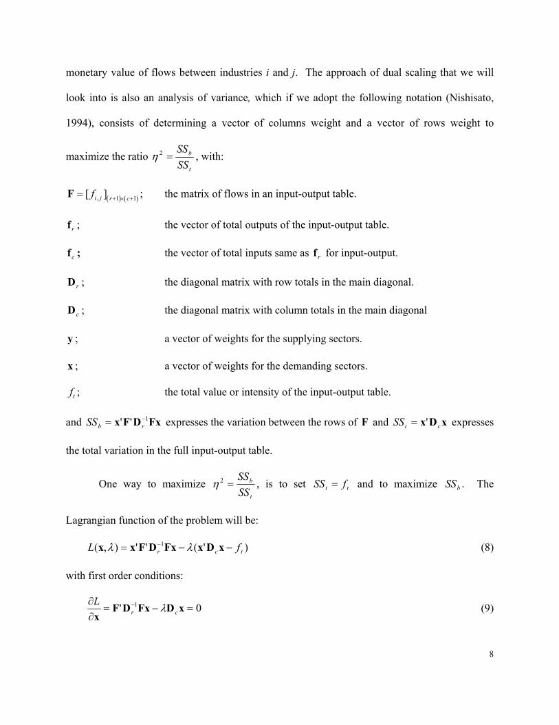
monetary value of flows between industries i and j. The approach of dual scaling that we will

look into is also an analysis of variance, which if we adopt the following notation (Nishisato,

1994), consists of determining a vector of columns weight and a vector of rows weight to

maximize the ratio t

b

SSSS

=2η , with:

( ) ( ), 1 1[ ]i j r cf + × +=F ; the matrix of flows in an input-output table.

rf ; the vector of total outputs of the input-output table.

cf ; the vector of total inputs same as rf for input-output.

rD ; the diagonal matrix with row totals in the main diagonal.

cD ; the diagonal matrix with column totals in the main diagonal

y ; a vector of weights for the supplying sectors.

x ; a vector of weights for the demanding sectors.

tf ; the total value or intensity of the input-output table.

and FxDFx 1'' −= rbSS expresses the variation between the rows of F and xDx ctSS '= expresses

the total variation in the full input-output table.

One way to maximize t

b

SSSS

=2η , is to set tt fSS = and to maximize bSS . The

Lagrangian function of the problem will be:

)'(''),( 1tcr fL −−= − xDxFxDFxx λλ (8)

with first order conditions:

0' 1 =−=∂∂ − xDFxDF

x crL λ (9)

9

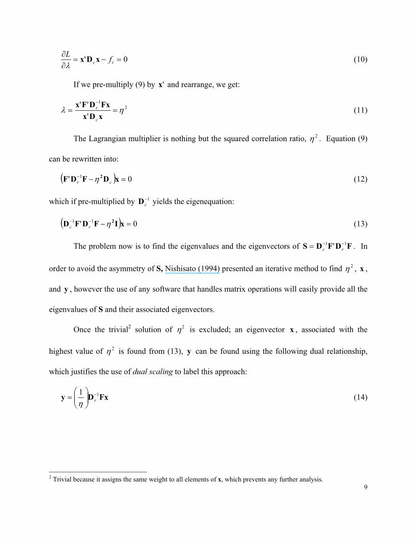
0' =−=∂∂

tc fL xDxλ

(10)

If we pre-multiply (9) by 'x and rearrange, we get:

21

'''

ηλ ==−

xDxFxDFx

c

r (11)

The Lagrangian multiplier is nothing but the squared correlation ratio, 2η . Equation (9)

can be rewritten into:

( ) 0' 1 =−− xDFDF 2cr η (12)

which if pre-multiplied by 1−cD yields the eigenequation:

( ) 0' 11 =−−− xIFDFD 2ηrc (13)

The problem now is to find the eigenvalues and the eigenvectors of FDFDS 11 ' −−= rc . In

order to avoid the asymmetry of S, Nishisato (1994) presented an iterative method to find 2η , x ,

and y , however the use of any software that handles matrix operations will easily provide all the

eigenvalues of S and their associated eigenvectors.

Once the trivial2 solution of 2η is excluded; an eigenvector x , associated with the

highest value of 2η is found from (13), y can be found using the following dual relationship,

which justifies the use of dual scaling to label this approach:

FxDy 11 −

= rη

(14)

2 Trivial because it assigns the same weight to all elements of x, which prevents any further analysis.

10

At this level, we obtain what is referred to as the first solution with a percentage of total

information explained of 21

1 2

100

ii

ηδ

η=∑

. Nishisato (1994) offers a different formulation to 1δ , but

it provides the same result since every eigenvalue explains part of the association and the sum of

the non-trivial eigenvalues exhausts all the association. If the first solution is judged insufficient

to explain the correlation between rows and columns then a second or more solutions can be

found by calculating the associated eigenvector x, and the vector y, by taking decreasing non-

trivial eigenvalues. In a general contingency ( )1r + -by- ( )1c + table, the number of possible

non-trivial solutions is min( , )s r c= .

Nishisato (1994) used an iterative method to find the eigenvalues, and the weights x and

y. However, the use of a non-iterative method but consistent with the method provided above

will provide a different set of x and y eigenvectors. The differences in results should not matter

because they stem mainly from the algorithm used by various software packages and all

eigenvectors correspond to the same eigenvalues3.

We mentioned earlier that the maximum number of solutions we can find is min( , )r c ,

and since the number of rows and columns in an input-output table are equal, then the number of

solutions is simply r or c , which is the size of the technical block matrix in an input-output

system. In determining the row and column weight vectors x and y , we will consider all the

solutions; in so doing, we can capture the full association between rows and columns. Once the

row and column weight vectors x and y are determined, many results can be extracted

3 For a given eigenvalue, different software packages produce different eigenvectors that are co-linear.

11

regarding the similarity within supplying industries and demanding industries on the one hand

and the associations between the supplying sectors and the demanding sectors on the other.

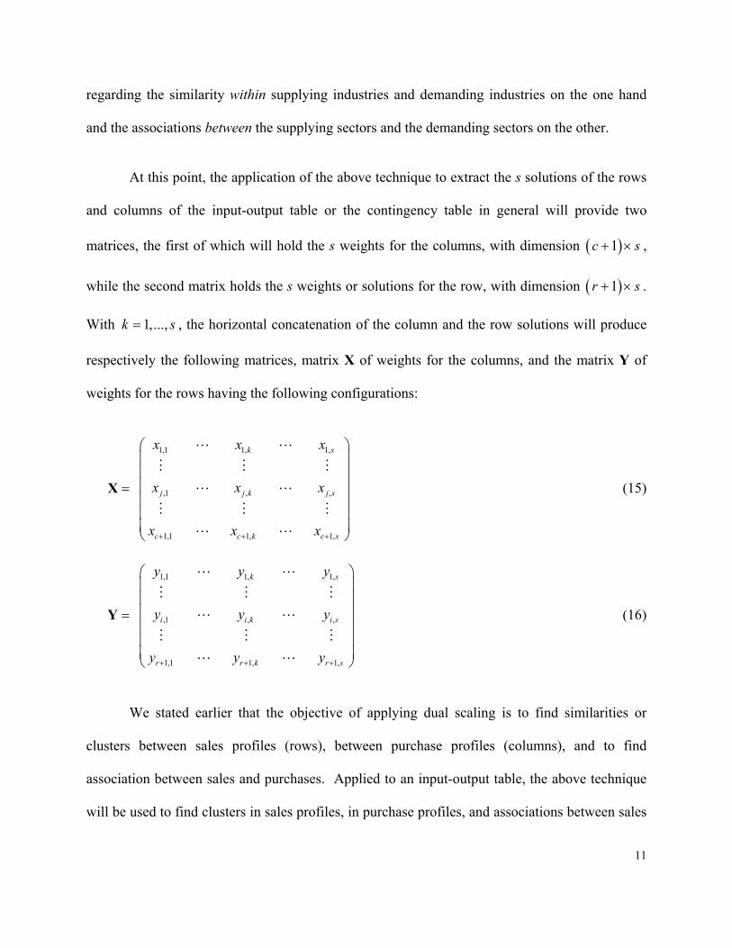
At this point, the application of the above technique to extract the s solutions of the rows

and columns of the input-output table or the contingency table in general will provide two

matrices, the first of which will hold the s weights for the columns, with dimension ( )1c s+ × ,

while the second matrix holds the s weights or solutions for the row, with dimension ( )1r s+ × .

With 1,...,k s= , the horizontal concatenation of the column and the row solutions will produce

respectively the following matrices, matrix X of weights for the columns, and the matrix Y of

weights for the rows having the following configurations:

1,1 1, 1,

,1 , ,

1,1 1, 1,

k s

j j k j s

c c k c s

x x x

x x x

x x x+ + +

=

X (15)

1,1 1, 1,

,1 , ,

1,1 1, 1,

k s

i i k i s

r r k r s

y y y

y y y

y y y+ + +

=

Y (16)

We stated earlier that the objective of applying dual scaling is to find similarities or

clusters between sales profiles (rows), between purchase profiles (columns), and to find

association between sales and purchases. Applied to an input-output table, the above technique

will be used to find clusters in sales profiles, in purchase profiles, and associations between sales

12

and purchases; in order to achieve this, we will disregard the primary inputs (last row) and the

final demand (last column) from any further analysis.

The matrices X and Y can be used to compute Euclidian rows-columns distances in the

space of dimension s. Computing the rows-columns distance implies that the weights ,j kx and

,i ky span the same Cartesian system of coordinates. The only trivial case where the rows and

columns weights are both in a Cartesian coordinate system of dimension s occurs when for a

given solution the correlation ratio 2η is equal to one, in which case there is a one-to-one match

between rows and columns weights, precluding any further study (Nishisato, 1994). Such a

situation is unlikely to happen for many contingency tables in general and for input-output tables

in particular, the reason being that it not possible to find an economy where each and every

industry's output is used as input only by the same industry and for final demand and all the rest

of inputs for every industry are coming exclusively from the primary factors. If such a situation

exists, the matrix of interindustry flows will be a diagonal matrix.

If we accept the unlikelihood of finding an economy whose interindustry matrix of flows

is diagonal, then in order to be able to compute the distance between row and column weights we

need to use a different expression of weights for the rows or the columns.4 For example, one

might proceed by projecting the row weights onto the axis of the column weights and use the

projection to compute the rows-columns distances. This procedure will ensure that both row and

column weights span the same coordinates system. We choose to keep the column weight as

found in (13) and use the projection of the row weights, which for a given solution transforms

(14) into:

4 Not doing so will be similar to drawing points in a system of coordinates with axes of different measurement units.

13

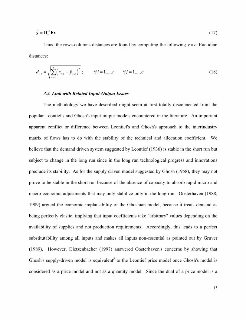
1ˆ r−=y D Fx (17)

Thus, the rows-columns distances are found by computing the following r c× Euclidian

distances:

( )2

, , ,1

ˆs

i j i k j kk

d x y=

= −∑ ; 1,...,i r∀ = 1,...,j c∀ = (18)

3.2. Link with Related Input-Output Issues

The methodology we have described might seem at first totally disconnected from the

popular Leontief's and Ghosh's input-output models encountered in the literature. An important

apparent conflict or difference between Leontief's and Ghosh's approach to the interindustry

matrix of flows has to do with the stability of the technical and allocation coefficient. We

believe that the demand driven system suggested by Leontief (1936) is stable in the short run but

subject to change in the long run since in the long run technological progress and innovations

preclude its stability. As for the supply driven model suggested by Ghosh (1958), they may not

prove to be stable in the short run because of the absence of capacity to absorb rapid micro and

macro economic adjustments that may only stabilize only in the long run. Oosterhaven (1988,

1989) argued the economic implausibility of the Ghoshian model, because it treats demand as

being perfectly elastic, implying that input coefficients take "arbitrary" values depending on the

availability of supplies and not production requirements. Accordingly, this leads to a perfect

substitutability among all inputs and makes all inputs non-essential as pointed out by Gruver

(1989). However, Dietzenbacher (1997) answered Oosterhaven's concerns by showing that

Ghosh's supply-driven model is equivalent5 to the Leontief price model once Ghosh's model is

considered as a price model and not as a quantity model. Since the dual of a price model is a

14

quantity model, then showing that Leontief and Ghosh models are equivalent price models,

implies that their duals are also equivalent. In addition to studies investigating the equivalence

of Leontief's and Ghosh's models, there is also a concern about their stability. In rejection of the

proportional filter approach of a direct comparison of the technical or allocation coefficients

across countries or periods, de Mesnard (1997) suggested a biproportional filtering method to

test the stability of the allocation and demand coefficients in comparative studies. Suppose that

we have to compare two matrices for the same economy at two different dates, such a

comparison is possible only if the margins are the same. The biproportional filtering approach

consists in transforming one of these matrices so that both matrices have the same row or column

margins to enable us to test the stability of Leontief's and Ghosh's coefficients. An alternative

way to compare two matrices might be through the comparison of the internal association

between their supply and demand sectors, especially that it involves both the demand and

allocations coefficients simultaneously. Indeed, if we reexamine equation (13), then the matrix

FDFDS 11 ' −−= rc will be shown to have elements of both Leontief's and Ghosh's models.

Let the matrix F from the contingency table be decomposed into the following block

matrix form, where the matrix Z of dimension r c× represents the interindustry flows, the row

vector V of dimension c represents the flows of primary inputs, and the column vector of the

flows of final demand C of dimension r :

( )( 1) ( 1)0 r c+ × +

=

Z CF

V (19)

The transpose of (19) gives:

5 Dietzenbacher (1997) compared their cost-push and demand-pull effects.

15

0′ ′ ′ = ′

Z VF

C (20)

With the matrices A and B of dimension r c× representing respectively the technical

coefficients and the demand coefficients blocks of the input-output table, v the row vector of

primary inputs coefficients, and d the final demand coefficients, if we premultiply (19) by 1r−D

and (20) by 1c−D we obtain:

1

0r−

=

B dD F

v (21)

and

1

0c− ′ ′ ′ = ′

A vD F

d (22)

Equations (21) and (22) are respectively Ghosh's supply driven model and the transpose

of Leontief's demand driven model; if we premultiply (22) by (21) then we will derive the S

matrix in equation (13), which can be expressed as a nonlinear combination of Leontief and

Ghosh models:

′ ′ ′ = ′ ′

A B + v v A dS

d B d d (23)

An appealing feature of dual scaling is its capacity to detect changes in the internal

association structure of input-output tables, even if the output, the final demand, and the

intermediary inputs remain unchanged.

Let = +H F ∆ , with P a perturbation matrix of dimension r c× that leaves the output

levels unchanged, the matrix ∆ has the following format:

( )( 1) ( 1)

00 0 r c+ × +

=

P∆ (24)

16

If we use the matrix H to compute a matrix 1 1c r− −′=S D H D H after the perturbation then we

obtain:

1 1 1 1 1 1c r c r c r− − − − − −′ ′ ′= + + +S S D ∆ D F D F D ∆ D ∆ D ∆ (25)

Form (25) it is clear that S and S are different, therefore their eigenvalues and

eigenvectors obtained from (13) are also different, meaning that all results (i.e. association loops)

based on the eigenvalues and the eigenvectors of S and S will be different. The differences

come from three sources: i) variations in the technical coefficients alone ( 1 1c r− −′D ∆ D F ); ii)

variations in the allocation coefficients alone ( 1 1c r− −′D F D ∆ ) and; iii) the combination of both

variations ( 1 1c r− −′D ∆ D ∆ ).

In the next section, we will apply the above method to the US and Canada input-output

tables and use the weight matrices x and y to computes the distance matrices from (18) in order

to compare the structure of associations between industries.

4. AN APPLICATION TO THE US AND CANADA 1995 INPUT-OUTPUT TABLES:

The log-linear regression, and the dual scaling method described above will be applied to

10-by-10 input-output tables6 of the US and Canada for 1995 in 1995 prices, where the values

are expressed in US million dollars. The details of the aggregation are provided in table A.1 in

the appendix.

6 The sectors considered are agriculture (AGR), mining (MNG), products of farms and diary (PFD), textiles (TXT), wearing apparel (CLG), ferrous metals (IRS), machinery and equipment (ME), transport equipment (TRE), other manufactured products (OMF), and services (SVC).

17

4.1. Log-linear Regression

A simple Chi-square test on the Canadian and US input-output tables transformed into

contingency tables shows, with no surprise, a rejection of the row-column independence

hypothesis. With a degree of freedom equal to a 100, and a computed Pearson Chi-square of

15,581,135.20 for the US and 1,083,322.87 for Canada, the rejection of the null hypothesis is

even stronger for the US; this indicates strong differences between the two economies' row-

column structure of dependence. The log-linear model will confirm with more detail the sources

and differences of dependencies in the input-output technical block of the two countries.

The results of the log-linear regression7 described in equation (6) are provided in table 1.

For the US, the results of the regression show that without interaction terms between the

variables, most individual effects of sales profiles are significant in explaining the volume of

exchange when independence is assumed. However there is a weak significance of the OMF and

a total absence of significance for the SVC. For the purchase profiles, the independence is

highly significant in the case of the OMF and the TRE. For Canada, the results are quite

different, where only the sales profile of the SVC seems to be insignificant in explaining the

volume of exchanges when row-column independence is assumed.

<< insert table 1 here >>

7 With 120 observations, for both Canada and the US, the correlation coefficient is high, 2 0.93R = .

18

Stronger evidence of association can be obtained through the scaled Pearson residuals

(SPR) in equation (7); in table 2 we provide for the US the value of the SPR for each cell and

highlight the values higher than 3 in absolute value, as recommended by Krzanowski (1998). A

similar table is provided for Canada in table 3.

<< insert table 2 here >>

<< insert table 3 here >> Comparing both tables, one notices that most of the association for the Canadian

economy is on the main diagonal and that the table 3 is sparse with few cells off the diagonal

where the association is high. Table 2, for the US is denser in cells of high association which is

expected knowing the different structure of both economies. Higher values of SPR denote the

failure of the row-column independence assumption and the higher the number of those cells the

healthier should be the economy. After a first assessment of the association in the interindustry

flows, a more elaborate and precise decomposition into different level of association will be used

next.

In relation to Simpson and Tsukui (1965) work on the block decomposition of input-

output tables, the existence of strong dependence along the main diagonal (see tables 2 and 3) is

a precursor sign of bloc independence that needs to be confirmed with more disaggregated data.

However, for both the US and Canada, the log-linear model does not show any signs of

triangularity while the bloc triangularity and the physical homogeneity of blocs need to be tested

with a more disaggregated data. At this level of aggregation, it is difficult to bridge the gap

between Simpson and Tsukui's results and our findings because a higher level of aggregation

although respecting the physical homogeneity will certainly suppress any information about the

bloc triangularity.

19

4.2. Dual Scaling

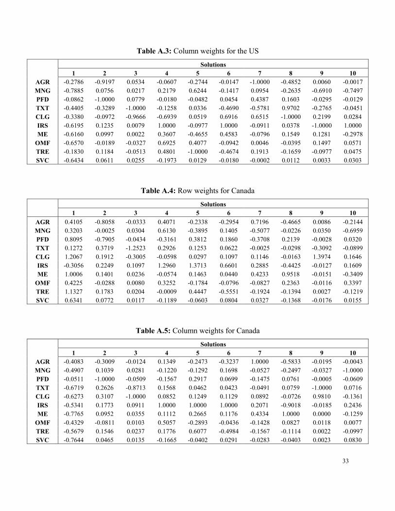
Using the dual scaling method, the maximum number of solutions for a (10+1)-by-(10+1)

complete input-output table8 is 10, which means that each sector of the weights can be plotted in

a space of dimension 10, where each solution occupies a dimension. The 10 solutions for the

weights for the supplying sectors (rows) and the demanding sectors (columns) for the US are

provided in tables A.2 and A.3 of the appendix, those for Canada are provided in tables A.4 and

A.5 of the appendix. While the focus of attention in this paper is not on a detailed examination

of the differences and similarities that are found in the two tables, some preliminary evaluation

will be made. Recall that the primary focus is a demonstration of the use of the dual scaling

technique in extracting information about the structure of input-output tables. The US-Canada

comparison offers a small insight into the type of information that can be gleaned from the

application; obviously, greater value would be gained from a comparative analysis with much

more disaggregated tables.

So far, we examined similarities between sales profiles and between purchase profiles:

now we will examine the association or the dependences between certain sales and purchases,

which we consider the main contribution of the dual scaling technique. We will still use the

Euclidian distance criterion to examine elements of the technical coefficient matrix that are key

to the overall explanation of the dependence between rows and columns of the input-output table

or the contingency table in general. The distance measure we will use is provided in (18) and its

values are provided in table A.6 for the US and table A.7 for Canada, in the appendix.

The rows-columns' weight Euclidian distances (tables A.6 and A.7) can be decomposed

into levels of dependences: at each level, we will identify the row-column dependences when

20

they exist. The decomposition procedure, we will use is analogous to the 'Matrioshka Principle'9

first introduced by Sonis and Hewings (1990). However, unlike the 'Matrioshka principle' the

decomposition we will operate is based on the row-column dependences or associations instead

of their intensities. This can be considered as a 'reversed Matrioshka' where the smallest sets, the

most compact ones, representing the highest order of dependence, are extracted first, providing

what may be termed an 'inside-out' decomposition. In Sonis and Hewings (1990), using a 'top-

down' decomposition, the technical coefficients block was decomposed into hierarchical closed

feedback loops of decreasing intensities. The decomposition we will operate here yields open

and closed loops of decreasing order of association.

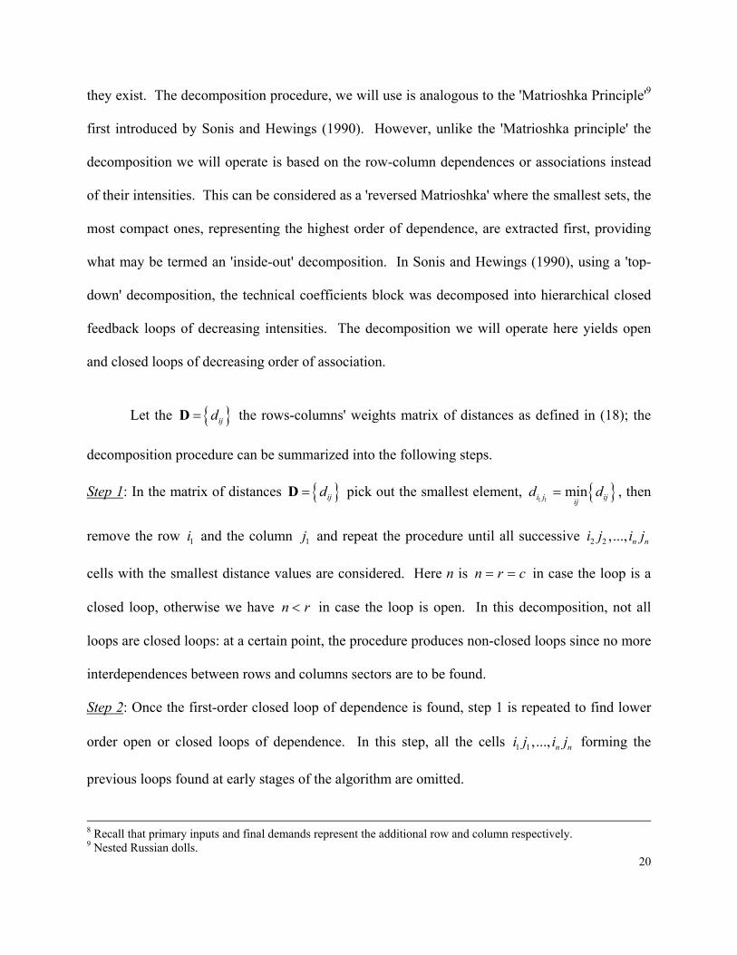
Let the { }ijd=D the rows-columns' weights matrix of distances as defined in (18); the

decomposition procedure can be summarized into the following steps.

Step 1: In the matrix of distances { }ijd=D pick out the smallest element, { }1 1mini j ijij

d d= , then

remove the row 1i and the column 1j and repeat the procedure until all successive 2 2 ,..., n ni j i j

cells with the smallest distance values are considered. Here n is n r c= = in case the loop is a

closed loop, otherwise we have n r< in case the loop is open. In this decomposition, not all

loops are closed loops: at a certain point, the procedure produces non-closed loops since no more

interdependences between rows and columns sectors are to be found.

Step 2: Once the first-order closed loop of dependence is found, step 1 is repeated to find lower

order open or closed loops of dependence. In this step, all the cells 1 1 ,..., n ni j i j forming the

previous loops found at early stages of the algorithm are omitted.

8 Recall that primary inputs and final demands represent the additional row and column respectively. 9 Nested Russian dolls.

21

To represent the association loops we will use the closed square brackets, [ ], to represent

closed loops and the open square brackets, ] [, to represent the open loops of associations. The

use of square brackets is preferable in order to avoid confusions with feedback loops

representation as in Sonis and Hewings (1990). When dealing with an open loop of association

the listing order of the different sectors of the loop matters, therefore we will consistently use the

arbitrary convention to always start open loops by a row sector.

The application of the two previous steps yields the various loops of dependence or

association shown in table 4 for the US and table 5 for Canada, where we also provide the

percentage of intensity captured by each association loop.

<< insert table 4 here >>

<< insert table 5 here >>

In a matrix of size n, open and closed loops of dependence have the following properties:

- The maximum length of a loop is n, where length should be interpreted as the number

of dependences or associations.

- When a loop of length n exists then it is closed.

- The maximum number of closed loops is n.

- The total length of all loops has to be 2n .

If we consider the decompositions obtained in table 4 and table 5, the difference in the total

length of loops denotes a lower dependence between supplying sectors and demanding sectors in

the Canadian economy compared to the US economy. In cases where open loops of dependence

exist, then reaching a higher order of dependence implies finding more associations in the

economy.

22

Tables 6 and 7 provide the full decompositions of the row-column weight distances for the

US and Canada, cells bearing the same number belong to the same association loop.

<< insert table 6 here >>

<< insert table 7 here >>

A careful look at tables 6 and 7 allows us to extract information about the technological

environment and market conditions each sector is facing. If we take table 6, and decide to

examine the technological environment of the textile industry (TXT), we notice that it is

primarily dependent on the supply of products of textile (TXT), then on services (SVC), etc…

The market conditions faced by the textile industry are that other than its own final demand, the

industry depends primarily on the demand of the textile industry (TXT), and then on the demand

of the transport equipment (TRE) industry, etc…

For Canada, table 7 reveals that textile industry (TXT) purchases depend primarily on the

supply the machinery and equipment industry (ME), then on the supply of transport equipment

(TRE), etc …The supply of the textile industry (TXT), depends primarily on the demand of the

services industry (SVC), then on the demand of the transport equipment industry (TRE), etc…

The difference in the demand dependence of the textile industry between Canada and the US

may be explained by the fact that cotton and wool production is more developed in the US than

in Canada. The differences observed in supply dependence of textiles can be explained by the

fact that most of the clothing products in the US are made in developing countries were labor is

cheaper, whereas Canada seems to have kept an industry for producing clothing apparel (CLG),

most likely to meet a specific local demand.

23

4.3. Economic Complexity

Unlike the top-down decomposition (Sonis and Hewings, 1990), the intensities of

association loops do not depict any particular order; in fact, what matters here is the intensity

accumulation occupied by each association loop. In the last columns of tables 4 and 5, we

provide the intensity accumulation of each association loop, those cumulative distribution of

intensities show the existence of evident cut-off points for the Canadian and US economies. The

approach we used to detect cut-off points is based on the observation of loops starting from

which a major change in the marginal intensity is observed. Before the cut-off loops, all marginal

intensities do not show a major change in the structure of the curve in figure 1. For the US

economy the two natural cut-off points seem to exist at the 5th and 8th loop, while for the

Canadian case the cut-off points exist at the 7th and 8th loops. Figure 1, shows that for the US

economy, the first level of loops represents 41.5% of the total interindustry flows and the total

length of the five first loops is 48. For Canada, the first level of loops occupies 59.2% of the

interindustry flows with a total loop length of 64, the qualitative difference between the two

economies founds explanation in the difference of economic structure and complexity of the two

economies, it is to be expected that the American economy is more integrated and complex than

the Canadian economy.

<< insert figure 1 here >>

Figure 1 shows that the second set of loops occupies for 55% of the interindustry flows

and the total length of the 3 loops is 26. For Canada, the second set of loops is relatively shorter

and occupies only 1 loop of length 10 but represents about 34.5% of the interindustry flows. The

last set of loops is relatively similar for Canada and the US and in both cases it occupies the last

7 loops whose total length is 26 and represent 3.6% of the interindustry flows for the US and

24

6.1% of those flows for Canada. Depending on the level of aggregation used in the input-output

table, it is expected that for most economies the interindustry complexity is decomposed into a

finite number of major stages. In our case, the first level of exchanges tends to lay down the

foundation of the economic system; the second level to bring the system to denser exchanges and

the last level takes the interindustry exchanges to a relative maturity.

5 CONCLUSION

Revealing the similarities in sectoral profiles and interpreting the linkages and the

internal associations in input-output systems is important for economic policy and for attempts to

predict their effects. It is in that spirit that in this paper we applied the log-linear model and the

dual scaling technique to identify cells where strong association exists and to construct open and

closed loops of associations. The association loops should be viewed as an additional tool along

with feedback loops and field of influence techniques to understand some of the details of the

finer structure of interindustrial dependences. The association loops as we showed above allow

for a crude decomposition of the economic complexity of interindustry flows.

The main purpose of the paper was to use the dual scaling technique to uncover the

associations between demand and supply in an interindustry exchange system. The association

loops that we constructed provide additional information about the dependences between supply

and demand, and allow for a relative classification of the sectors' dependences and those patterns

can be compared across time and space. We stated above that the usefulness of the association

loops is that they allow for the study of more specific sources of change such as demand or

supply in an industry as a whole, rather than a change in coefficients without further knowledge

of the source of change especially in cases where the source could be a change in the

technological and/or market conditions. While the advantage of using the association loops is to

25

obtain a relative hierarchical decomposition of dependencies, it is not possible to reveal their

magnitudes as in the field of influence theory. A gain in the understanding of economies through

input-output systems could be achieved if a way can be found to relate the association loops and

the field of influence so that both the magnitudes of changes and their hierarchy are represented.

Such a linkage might be considered as the development of elasticities of sales and purchases

relating to all the elements in the technical block matrix.

Further applications could be made to reveal the evolution of structural change in a single

economy over time, or, in parallel to the application illustrated in this paper, to economies at

similar stages of development.

REFERENCES

Cella, G. (1984) The Input-Output Measurement of Interindustry Linkages, Oxford

Bulletin of Economics and Statistics, 46, pp. 73-84.

Cella, G. (1986) The Input-Output Measurement of Interindustry Linkages: A Reply,

Oxford Bulletin of Economics and Statistics, 48, pp. 379-384.

Clements, B. J. (1990) On the Decomposition and Normalization of Interindustry

Linkages, Economics Letters, 33, pp. 337-340.

De Mesnard, L. (1997) A Biproportional Filter to Compare Technical and Allocation

Coefficients Variations, Journal of Regional Science, 37, pp. 541-564.

Dietzenbacher, E. (1997) In Vindication of the Ghosh Model: A Reinterpretation of a

Price Model, Journal of Regional Science, 37, pp. 629-651.

Ghosh, A. (1958) Input-Output Approach in an Allocation System, Economica, 25, pp.

58-64.

26

Gruver, G. W (1989) On the Plausibility of the Supply-Driven Input-Output Model: A

Theoretical Basis for the Input-Coefficient Change, Journal or Regional Science, 3, pp. 441-450.

Hirschman, A. O. (1958) The Strategy of Economic Development, (New Haven, Yale

University Press).

Krzanowski, W. (1998) An Introduction to Statistical Modeling, (London, Arnold), Ch. 5

and 7.

Leontief, W. W. (1936) Quantitative Input and Output Relations in the Economic

Systems of the United States, Review of Economic Statistics, 18, pp. 105-125.

Nishisato, S. (1980) Analysis of Categorical Data: Dual Scaling and its Applications,

(Toronto, University of Toronto Press).

Nishisato, S. (1994) Elements of Dual Scaling: An Introduction to Practical Data

Analysis, (New Jersey, Lawrence Erlbaum Associates).

O'Huallachain, B. (1984) The Identification of Industrial Complexes, Annals of the

Association of American Geographers, 74, pp. 420-436.

Oosterhaven, J. (1988) On the Plausibility of the Supply-Driven Input-Output Model,

Journal of Regional Science, 28, pp. 203-217.

Oosterhaven, J. (1989) The Supply-Driven Input-Output Model: A New Interpretation

but still Implausible, Journal or Regional Science, 3, pp. 459-465.

Rasmussen, P. N. (1956) Studies in Inter-Sectoral Relations, (Amsterdam, North-Holland

Publishing).

Simpson, D. & J. Tsukui (1965) The Fundamental Structure of Input-Output Tables, An

International Comparison, Review of Economics and Statistics, 47, pp. 434-446.

27

Sonis, M. & G. J.D. Hewings (1990) The 'Matrioshka Principal' in the Hierarchical

Decomposition of Multi-regional Social Accounting Systems, in Anselin, L. & M. Madden (eds.)

New Directions in Regional Analysis: Integrated and Multi-Regional Approaches, (London,

Belhaven Press), Ch. 7, pp. 101-111.

Sonis, M. & G. J.D. Hewings (1992) Coefficient Change in Input-Output Models: Theory

and Applications, Economic Systems Research, 4, pp. 143-157.

Sonis, M. & G. J.D. Hewings (1993) Hierarchies of Regional Sub-Structures and their

Multipliers within Input-Output Systems: Miyazawa Revisited, Hitotsubashi Journal of

Economics, 34, pp. 33-44.

Sonis, M. & G. J.D. Hewings (1999) Economic Landscapes: Multiplier Product Matrix

Analysis for Multiregional Input-Output Systems, Hitotsubashi Journal of Economics, 40, pp.

59-74.

Sonis, M. & G. J.D. Hewings (2000) Introduction to Input-Output Structural Q-Analysis,

Regional Economics Applications Laboratory-Technical Series: REAL 00-T-1.

Sonis, M., G. J.D. Hewings, & J. Guo (1996) Sources of Structural Changes in Input-

Output Systems: A Field of Influence Approach, Economic Systems Research, 8, pp. 15-32.

Sonis, M., G. J.D. Hewings, & J. Guo (2000) A New Image of Classical Key Sector

Analysis: Minimum Information Decomposition of the Leontief Inverse, Economic Systems

Research, 12, pp. 401-423.

Sonis, M., J. J.M. Guilhoto, G. J.D. Hewings & E. B. Martins (1995) Linkages, Key

Sectors and Structural change: Some New Perspectives, The Developing Economies, 33, pp. 233-

270.

28

Table 1: Log-linear model US rows CA rows US cols CA cols

m 6.908 6.0699 m 6.908 6.0699 (15.92)*** (18.00)*** (15.92)*** (18.00)***

x1 -1.7394 -1.6918 y1 -2.5473 -2.4998 (3.54)*** (4.44)*** (5.86)*** (7.40)***

x2 -2.277 -2.1323 y2 -1.5971 -1.5492 (4.62)*** (5.57)*** (3.66)*** (4.57)***

x3 -1.6948 -1.8494 y3 -2.4131 -2.1814 (3.44)*** (4.83)*** (5.53)*** (6.44)***

x4 -2.1634 -2.758 y4 -2.0801 -2.0103 (4.39)*** (7.21)*** (4.77)*** (5.93)***

x5 -2.5678 -3.0288 y5 -2.526 -2.2625 (5.21)*** (7.92)*** (5.79)*** (6.68)***

x6 -2.8724 -2.5765 y6 -3.2374 -3.1717 (5.83)*** (6.73)*** (7.42)*** (9.36)***

x7 -1.5465 -2.0873 y7 -1.589 -1.5673 (3.14)*** (5.45)*** (3.64)*** (4.63)***

x8 -0.9558 -1.1149 y8 -0.9525 -1.3331 (1.94)* (2.91)*** (2.18)** (3.94)***

x9 -1.8613 -1.7726 y9 -0.982 -0.9517 (3.78)*** (4.63)*** (2.25)** (2.81)***

x10 -0.3975 -0.7911 y10 -2.2608 -2.1095 (-0.81) (2.07)** (5.18)*** (6.23)***

Absolute value of t statistics in parentheses * significant at 10%; ** significant at 5%; *** significant at 1%

Table 2: Inter-industry flows association for the US: cells with strong rejection of the independence hypothesis

AGR MNG PFD TXT CLG IRS M E OMF TRE SVC AGR 27.76 -1.81 34.75 10.66 3.80 -1.85 -2.73 7.82 -3.38 -0.46 MNG -3.20 13.83 1.29 -2.08 -3.23 9.72 -0.64 6.50 0.67 11.22 PFD 9.07 -1.43 37.35 -1.63 -1.97 -1.20 -1.92 0.46 -3.76 5.61 TXT -1.74 -0.94 -2.84 19.24 21.54 -2.01 -0.36 4.20 9.71 -0.78 CLG -3.07 -1.50 -3.02 0.79 24.48 -0.91 -0.36 -1.67 -0.69 0.13 IRS -1.17 7.69 -1.56 -0.05 -0.52 14.19 6.40 1.82 4.60 -6.61 M E -0.61 3.92 -2.91 -2.04 -3.44 3.74 7.48 -6.43 5.79 -6.86 OMF -0.45 3.07 4.72 4.53 2.10 5.42 6.44 8.73 8.93 0.68 TRE -6.07 -5.27 -2.99 -2.71 -2.05 -1.02 0.73 -3.48 31.19 1.10 SVC 23.78 0.85 -3.29 -4.84 -2.55 3.40 -3.68 -8.70 -1.74 -4.40

29

Table 3: Inter-industry flows association for Canada: cells with strong rejection of the

independence hypothesis AGR MNG PFD TXT CLG IRS M E OMF TRE SVC

AGR 11.38 -1.18 16.37 -0.83 -0.34 -0.85 -1.42 10.52 -1.75 -0.42 MNG -2.42 3.86 -0.26 -0.21 -1.09 4.41 -0.41 5.36 -0.55 4.30 PFD 1.67 -1.28 19.15 -0.78 -0.28 -1.28 -1.06 -1.24 -2.45 2.79 TXT -1.17 -1.40 -1.63 9.58 11.21 -0.88 -1.28 0.34 1.31 -0.71 CLG -1.60 -0.80 -1.88 2.57 7.73 -0.47 -0.27 -0.11 -0.21 0.36 IRS -0.43 5.10 -0.73 -0.10 -0.65 8.12 4.13 0.37 3.88 -2.95 M E -1.08 1.45 -2.05 -1.14 -1.58 -0.42 5.62 -3.55 0.30 -2.43 OMF 2.64 2.77 4.30 1.45 0.60 2.34 3.48 4.64 1.97 0.65 TRE -4.02 -2.87 -1.91 -1.06 -0.96 -0.64 0.23 -2.34 14.04 -0.32 SVC 11.79 1.52 -2.76 -1.48 -0.69 -0.26 -1.59 -5.18 -3.23 -2.43

Table 4: Dependence Loops for the US and their Length

Order Closed / Open Loops Length % Intensity1

Cumul. Intensity

1 [AGR PFD] [MNG SVC] [TXT] [CLG] [IRS OMF ME TRE] 10 9.3118% 9.31% 2 [AGR][PFD][MNG OMF SVC TXT TRE CLG IRS ME] 10 13.9788% 23.29% 3 ]IRS SVC AGR MNG ME CLG[ [PFD TXT] [OMF] [TRE] 9 9.9812% 33.27% 4 [AGR OMF PFD IRS TRE] [MNG] [TXT SVC CLG] [ME] 10 4.6002% 37.87% 5 ]IRS MNG AGR SVC PFD CLG[ [TXT ME OMF TRE] 9 3.6908% 41.56% 6 ]IRS AGR ME TXT OMF MNG PFD TRE[ [SVC] 8 42.9235% 84.49% 7 ]IRS PFD OMF AGR TXT MNG TRE[ [ME SVC] 8 4.9308% 89.42% 8 [AGR TRE ME PFD SVC OMF TXT] [MNG CLG] [IRS] 10 6.9825% 96.40% 9 ]MNG TXT CLG PFD ME AGR[ ]OMF IRS[ [TRE SVC] 8 2.6952% 99.09% 10 ]TRE PFD MNG IRS TXT[ ]OMF CLG SVC[ 6 0.2645% 99.36% 11 ]AGR CLG TRE OMF[ ]TXT IRS[ 4 0.0271% 99.39% 12 ]AGR IRS CLG ME[ ]TRE MNG[ 4 0.0032% 99.39% 13 ]CLG OMF[ ]ME IRS[ 2 0.0969% 99.49% 14 ]CLG AGR[ ]SVC IRS[ 2 0.5135% 100%

Total 100 100% - 1) The intensities are computed as percentages of the interindustries flows

30

Table 5: Dependence Loops for Canada and their Length

Table 6: Decomposition into open and closed loops of sectors' dependences for the US AGR MNG PFD TXT CLG IRS ME OMF TRE SVC

AGR 2 3 1 7 11 12 6 4 8 5 MNG 5 4 6 9 8 10 3 2 7 1 PFD 1 10 2 3 5 4 9 7 6 8 TXT 8 7 3 1 9 11 5 6 2 4 CLG 14 8 9 4 1 2 12 13 11 10 IRS 6 5 7 10 12 8 2 1 4 3 ME 9 2 8 6 3 13 4 5 1 7

OMF 7 6 4 8 10 9 1 3 5 2 TRE 4 12 10 5 2 1 8 11 3 9 SVC 3 1 5 2 4 14 7 8 9 6

Order Closed / Open Loops Length % Intensity1

Cumul. Intensity

1 [AGR PFD ME TXT SVC] [MNG TRE IRS OMF] [CLG] 10 5.2710% 5.271% 2 [AGR] [PFD] [MNG OMF ME CLG IRS SVC] [TXT TRE] 10 13.3322% 18.603% 3 [AGR MNG SVC ME IRS TRE CLG TXT OMF PFD] 10 5.2412% 23.844% 4 [AGR SVC TRE ME] ]IRS MNG PFD CLG[ [TXT] [OMF] 9 11.2515% 35.096% 5 [AGR OMF SVC TXT MNG] ]IRS PFD TRE[ [ME] 8 10.3470% 45.443% 6 [AGR TXT PFD SVC OMF TRE] [MNG] ]IRS ME[ 8 10.3686% 55.811% 7 ]IRS AGR TRE MNG ME SVC PFD OMF TXT CLG[ 9 3.4004% 59.212% 8 [AGR ME OMF IRS TXT] [MNG CLG TRE PFD] [SVC] 10 34.6957% 93.908% 9 ]TRE OMF AGR IRS CLG SVC[ ]MNG TXT ME PFD[ 8 0.9991% 94.907% 10 ]PFD TXT[ [CLG OMF] [IRS] ]ME TRE SVC[ 6 1.3283% 96.235% 11 ]AGR CLG PFD[ ]ME MNG[ ]TXT IRS[ [TRE] 5 2.5265% 98.762% 12 ]SVC CLG MNG IRS[ 3 0.4509% 99.212% 13 ]CLG AGR[ ]SVC IRS[ 2 0.7860% 99.998% 14 ]PFD IRS[ ]CLG ME[ 2 0.0016% 100%

Total 100 100 % - 1) The intensities are computed as percentages of the interindustries flows

31

Table 7: Decomposition into open and closed loops of sectors' dependences for Canada

AGR MNG PFD TXT CLG IRS ME OMF TRE SVC AGR 2 3 1 6 11 9 8 5 7 4 MNG 5 6 4 9 8 12 7 2 1 3 PFD 3 8 2 10 4 14 1 7 5 6 TXT 8 5 6 4 7 11 9 3 2 1 CLG 13 12 11 3 1 2 14 10 8 9 IRS 7 4 5 8 9 10 6 1 3 2 ME 4 11 9 1 2 3 5 8 10 7

OMF 9 1 3 7 10 8 2 4 6 5 TRE 6 7 8 2 3 1 4 9 11 10 SVC 1 2 7 5 12 13 3 6 4 8

Figure 1: Characteristics of association loops

32

APPENDIX

Table A.1: Input-output aggregation for the US and Canadian economies

Aggregate Description Aggregate Description Paddy rice TXT Textiles Wheat CLG Wearing apparel Cereal grains IRS Ferrous metals Vegetables, fruit, nuts Electronic equipment Oil seeds

M E Machinery and equipment

Sugar cane, sugar beet Motor vehicles and parts Plant-based fibers

TRE Transport equipment

Crops Leather products Bovine cattle, sheep and goats Wood products Wool, silk-worm cocoons Paper products, publishing Forestry Petroleum, coal products Fishing Chemical, rubber, plastic products

AGR

Processed rice Metals Coal Metal products Oil

OMF

Manufactures Gas Electricity Minerals Gas manufacture, distribution

MNG

Mineral products Water Animal products Construction Raw milk Trade, transport Bovine cattle, sheep and goat Financial, business, recreational services Meat products Public admin and defense, education, health Vegetable oils and fats

SVC

Dwellings Dairy products Sugar

PFD

Food products

Table A.2: Row weights for the US

Solutions 1 2 3 4 5 6 7 8 9 10

AGR 0.1532 -1.5492 0.0533 0.0825 -0.2333 -0.0007 -0.5972 -0.2973 -0.0364 -0.0235 MNG -0.8572 0.0162 0.0060 0.8655 1.0956 -0.2039 0.1585 -0.2910 -0.6086 -0.4863 PFD 0.7635 -0.5704 0.0693 -0.1259 0.0417 0.0849 0.6675 0.2929 -0.0535 -0.0003 TXT 0.0175 -0.2347 -1.3112 -0.3445 -0.0277 -0.1520 -0.1743 0.4536 -0.2589 -0.0407 CLG 1.1722 0.0357 -0.4284 -0.4558 0.1893 0.8366 0.7587 -1.3339 0.3973 0.0376 IRS -0.7859 0.1511 -0.0349 1.9061 -0.5781 1.1782 -0.0810 0.1265 -0.5694 0.8815 ME 0.7229 0.1204 0.0048 0.2601 -0.4870 0.2822 -0.0693 0.0910 0.0631 -0.4559

OMF -0.1008 -0.0389 -0.0457 0.6121 0.1892 -0.1467 0.0259 0.0392 0.2841 0.0398 TRE 1.1284 0.1280 -0.0139 0.2676 -0.8309 -0.5391 0.1927 -0.2217 -0.1703 0.0934 SVC 0.6626 0.0601 0.0173 -0.0952 0.1086 0.0113 -0.0641 0.0100 -0.0163 0.0368

33

Table A.3: Column weights for the US

Solutions 1 2 3 4 5 6 7 8 9 10

AGR -0.2786 -0.9197 0.0534 -0.0607 -0.2744 -0.0147 -1.0000 -0.4852 0.0060 -0.0017 MNG -0.7885 0.0756 0.0217 0.2179 0.6244 -0.1417 0.0954 -0.2635 -0.6910 -0.7497 PFD -0.0862 -1.0000 0.0779 -0.0180 -0.0482 0.0454 0.4387 0.1603 -0.0295 -0.0129 TXT -0.4405 -0.3289 -1.0000 -0.1258 0.0336 -0.4690 -0.5781 0.9702 -0.2765 -0.0451 CLG -0.3380 -0.0972 -0.9666 -0.6939 0.0519 0.6916 0.6515 -1.0000 0.2199 0.0284 IRS -0.6195 0.1235 0.0079 1.0000 -0.0977 1.0000 -0.0911 0.0378 -1.0000 1.0000 ME -0.6160 0.0997 0.0022 0.3607 -0.4655 0.4583 -0.0796 0.1549 0.1281 -0.2978

OMF -0.6570 -0.0189 -0.0327 0.6925 0.4077 -0.0942 0.0046 -0.0395 0.1497 0.0571 TRE -0.1830 0.1184 -0.0513 0.4801 -1.0000 -0.4674 0.1913 -0.1659 -0.0977 0.0475 SVC -0.6434 0.0611 0.0255 -0.1973 0.0129 -0.0180 -0.0002 0.0112 0.0033 0.0303

Table A.4: Row weights for Canada

Solutions 1 2 3 4 5 6 7 8 9 10

AGR 0.4105 -0.8058 -0.0333 0.4071 -0.2338 -0.2954 0.7196 -0.4665 0.0086 -0.2144 MNG 0.3203 -0.0025 0.0304 0.6130 -0.3895 0.1405 -0.5077 -0.0226 0.0350 -0.6959 PFD 0.8095 -0.7905 -0.0434 -0.3161 0.3812 0.1860 -0.3708 0.2139 -0.0028 0.0320 TXT 0.1272 0.3719 -1.2523 0.2926 0.1253 0.0622 -0.0025 -0.0298 -0.3092 -0.0899 CLG 1.2067 0.1912 -0.3005 -0.0598 0.0297 0.1097 0.1146 -0.0163 1.3974 0.1646 IRS -0.3056 0.2249 0.1097 1.2960 1.3713 0.6601 0.2885 -0.4425 -0.0127 0.1609 ME 1.0006 0.1401 0.0236 -0.0574 0.1463 0.0440 0.4233 0.9518 -0.0151 -0.3409

OMF 0.4225 -0.0288 0.0080 0.3252 -0.1784 -0.0796 -0.0827 0.2363 -0.0116 0.3397 TRE 1.1327 0.1783 0.0204 -0.0009 0.4447 -0.5551 -0.1924 -0.1394 0.0027 -0.1219 SVC 0.6341 0.0772 0.0117 -0.1189 -0.0603 0.0804 0.0327 -0.1368 -0.0176 0.0155

Table A.5: Column weights for Canada

Solutions 1 2 3 4 5 6 7 8 9 10

AGR -0.4083 -0.3009 -0.0124 0.1349 -0.2473 -0.3237 1.0000 -0.5833 -0.0195 -0.0043 MNG -0.4907 0.1039 0.0281 -0.1220 -0.1292 0.1698 -0.0527 -0.2497 -0.0327 -1.0000 PFD -0.0511 -1.0000 -0.0509 -0.1567 0.2917 0.0699 -0.1475 0.0761 -0.0005 -0.0609 TXT -0.6719 0.2626 -0.8713 0.1568 0.0462 0.0423 -0.0491 0.0759 -1.0000 0.0716 CLG -0.6273 0.3107 -1.0000 0.0852 0.1249 0.1129 0.0892 -0.0726 0.9810 -0.1361 IRS -0.5341 0.1773 0.0911 1.0000 1.0000 1.0000 0.2071 -0.9018 -0.0185 0.2436 ME -0.7765 0.0952 0.0355 0.1112 0.2665 0.1176 0.4334 1.0000 0.0000 -0.1259

OMF -0.4329 -0.0811 0.0103 0.5057 -0.2893 -0.0436 -0.1428 0.0827 0.0118 0.0077 TRE -0.5679 0.1546 0.0237 0.1776 0.6077 -0.4984 -0.1567 -0.1114 0.0022 -0.0997 SVC -0.7644 0.0465 0.0135 -0.1665 -0.0402 0.0291 -0.0283 -0.0403 0.0023 0.0830

34

Table A.6: Row-column weights Euclidian distances for the US

AGR MNG PFD TXT CLG IRS ME OMF TRE SVC AGR 1.1792 1.6815 0.7198 1.7250 1.9740 2.2299 1.2718 1.2565 1.4208 1.0086MNG 1.5716 1.1182 1.2507 1.6958 1.9416 1.9363 0.9163 0.5858 1.3702 0.4698PFD 1.6155 1.8200 1.0530 1.8870 2.0081 2.3288 1.4322 1.4478 1.4626 1.1841TXT 1.5323 1.5836 1.1634 1.4126 1.6981 2.2012 1.1815 1.2030 1.3597 0.8318CLG 1.8434 2.0119 1.4238 2.0991 1.9073 2.4719 1.6514 1.6970 1.6378 1.4320IRS 1.6097 1.3814 1.3362 1.7872 2.0439 1.6766 0.6613 0.6597 1.1772 0.7182ME 1.6653 1.7944 1.2787 1.8968 2.0328 2.2512 1.3039 1.3965 1.3366 1.1477

OMF 1.5017 1.4355 1.1123 1.6887 1.9171 2.0383 0.9830 0.9000 1.2196 0.6824TRE 1.8027 2.0017 1.4159 2.0364 2.1636 2.4119 1.5612 1.6271 1.4009 1.4077SVC 1.6423 1.7465 1.2436 1.8611 1.9898 2.2729 1.3497 1.3716 1.4053 1.0866

Table A.7: Rows-column weights Euclidian distances for Canada AGR MNG PFD TXT CLG IRS ME OMF TRE SVC

AGR 1.3376 1.3573 0.9664 1.7115 1.7659 2.1555 1.5966 0.9008 1.2503 1.1123MNG 1.4304 1.2790 1.1430 1.6290 1.6921 2.0962 1.5334 0.7959 1.1779 1.0287PFD 1.6050 1.5181 1.0135 1.8720 1.9143 2.2921 1.7652 1.2002 1.4266 1.3422TXT 1.4210 1.2593 1.2104 1.3863 1.4383 2.0682 1.4625 0.8513 1.0924 0.9443CLG 1.7654 1.6777 1.4083 1.9979 1.9757 2.3936 1.9490 1.3923 1.6143 1.5799IRS 1.3591 1.2037 1.1840 1.4621 1.5281 1.7148 1.2688 0.6738 0.8160 0.7761ME 1.6815 1.5805 1.3152 1.9096 1.9460 2.3366 1.7918 1.2729 1.4959 1.4469

OMF 1.4437 1.3317 1.1339 1.6637 1.7232 2.1437 1.5534 0.8916 1.2065 1.0781TRE 1.7388 1.6472 1.3674 1.9724 2.0037 2.3585 1.9121 1.3551 1.5162 1.5354SVC 1.5196 1.3965 1.1902 1.7515 1.7952 2.2128 1.6639 1.0643 1.3123 1.1983