J Comb Optim (2008) 15: 287–304DOI 10.1007/s10878-007-9103-3

A simulation tool for modeling the influence of anatomyon information flow using discrete integrate and fireneurons

Maya Maimon · Larry Manevitz

Published online: 4 October 2007© Springer Science+Business Media, LLC 2007

Abstract There are theories on brain functionality that can only be tested in verylarge models. In this work, a simulation model appropriate for working with largenumber of neurons was developed, and Information Theory measuring tools weredesigned to monitor the flow of information in such large networks. The model’ssimulator can handle up to one million neurons in its current implementation by usinga discretized version of the Lapicque integrate and fire neuron instead of interactingdifferential equations. A modular structure facilitates the setting of parameters of theneurons, networks, time and most importantly, architectural changes.

Applications of this research are demonstrated by testing architectures in terms ofmutual information. We present some preliminary architectural results showing thatadding a virtual analogue to white matter called “jumps” to a simple representation ofcortex results in: (1) an increase in the rate of mutual information flow, correspondingto the “bias” or “priming” hypothesis; thereby giving a possible explanation of thehigh speed response to stimuli in complex networks. (2) An increase in the stabilityof response of the network; i.e. a system with “jumps” is a more reliable machine.This also has an effect on the potential speed of response.

Keywords Large scale neural simulator · Temporal discrete integrate and fire ·Information theory · Bias or priming hypothesis

1 Introduction

It is well known that the human cortex is extremely large in terms of the numberof neurons (Braitenberg and Schüz 1998). As a result, there are theories about its

M. Maimon · L. Manevitz (�)Department of Computer Science, University of Haifa, Haifa, Israele-mail: manevitz@cs.haifa.ac.il

M. Maimone-mail: mayam@cs.haifa.ac.il

288 J Comb Optim (2008) 15: 287–304

function which can only be tested in very large models. One standard approach is touse “in vivo” models, i.e. animal models. Another approach is to use “ex vivo” models(Marom and Shahaf 2002), i.e cortical neurons that are grown in a petri dish andelectronically monitored and stimulated. An advantage of these models is that theyseem to have the same neuronal functionality as the human cortex; a disadvantage isthat they are not subject to complete control and thus are not suitable, for example, toexplore variants of architectural structure.

Thus, there is an important place for formal models of neurons and neural net-works. These models, although necessarily highly caricatured and simplified pro-vide a way to understand, both in theoretical results and in simulations, informationprocessing principles in the brain. In fact, its very simplicity, rather than a defect, canin certain instances be thought of as an abstraction of natural networks. Thus, if acertain part of processing can be understood at this level of abstraction, it shows thatfurther details are unnecessary to explain the natural phenomenon.

In addition, of course, such computational models allow the study of differentaspects; e.g. of conduction or architecture independently of the myriad other para-meters. Such models have been used by many researchers, such as Rolls et al, Deco,Panzeri, Abbott and Marom (Abbott 1999; Panzeri et al. 1999; Rolls et al. 2003;Marom and Shahaf 2002; Treves et al. 1997; Trappenberg 2002). Despite their rel-ative simplicity to natural models, the interactions of such artificial neurons can bevery complex; and researchers are forced to make simplifying choices in their mod-eling tools.

It is well established that the simplest of such models, networks based on theMcCullough–Pitts model of the neuron do not contain sufficient information. Whilethey can be used to good effect to study certain aspects of connectivity and so on,they lack any aspect of temporal effects and relationships.

The most famous “realistic” models of the neuron are the primitive Lapicque In-tegrate and Fire neuron (Lapicque 1907) and its successors and the more descriptivemodels based on the famous Hodgkin–Huxley model (Hodgkin and Huxley 1952).The latter, being a complex interaction of several differential equations is mostlythought to be too complex to use in large scale models; and the typical applicationtends to use a version of the integrate and fire model. Nonetheless, the Lapicquemodel itself involves differential equations, and modeling large scale requires the in-teractions between a huge number of such equations. Such a system can not be solvedanalytically (thereby, removing one of the compelling reasons to model with suchequations); but must be solved numerically. This is possible, but involves numerousquestions of numerical analysis.

In this work, we make the simplifying assumption to work with a discretized ver-sion of the integrate and fire neuron; thus our model of the network can be thoughtof as a version of a complex “cellular automaton”; where each cell is one of ourneurons; but the connections are more complex than are usually modeled in suchautomata (Wolfram 2002).

This simplified model maintains at the level of the neurons the temporal effect, andwe find that working with such a model is simpler both logically and computation-ally. If it is accepted that the important information from a computational perspectiveis represented in such temporally discrete neurons, the computational challenges aremitigated and there is a huge computational reduction. Thus experimentation with

J Comb Optim (2008) 15: 287–304 289

different parameters, architectures and encodings can be accomplished in a reason-able time.

This idea is demonstrated here with the development of a version of a computa-tional tool. Changing, for example, the architecture of the network (which generatesthe spike history of the neurons) can be done by simply changing parameters duringthe processing of the model.

The current implementation (the second such) works on a dual 64 bit-processor2.4 MHz AMD with 16 Gigabytes of internal memory. On this machine, in principle50 million neurons can be implemented. We actually experimented with as many asone million neurons; although most of our results were done with “small” networksof 10,000 to 100,000 neurons.

Monitoring such a large network carries its own problems. A central tool we de-cided to implement1 is to use information theoretic measures, in particular the rate offlow of mutual information.

This is accomplished by implementing the ideas of Treves, Panzeri, Shultz, Trevesand Rolls (Panzeri et al. 1999) which we describe in Sect. 3.

In our preliminary experiments we investigated the effect of changing the archi-tecture of a rectangular piece of “cortex” allowing or disallowing “jumps” which, insome sense correspond to an interpretation of white matter.

The results show: (1) more connections (“dendrites”) results in faster mutual in-formation, meaning the mutual information is higher earlier in time. Firing rates arehigher and faster. That is, the spikes occur earlier in time, producing the informationfaster. The additional connections increase the chance to emit spikes, resulting in ahigher firing rate and faster rate of mutual information. (2) The use of “jumps” verifiesthe “bias” hypothesis; i.e. a small number of forward jumps, as opposed to “percola-tions” of information, causes the mutual information curve to rise much faster. Thishelps to explain how responses can be so fast in such complex networks. (3) The useof “jumps” also results in a more stable and predictive network which has many pos-sible consequences; including allowing more reliable guesses of the stimulus. Thisimplies that it is possible for the cortex to function by making early guesses as to thetotal incoming signal; only correcting when necessary.

2 The modeled neuron and networks

2.1 The neuron

The main functionality of the neuron that we are interested in was modeled byLapicque in the integrate and fire neuron (I&F) (Abbott 1999) using a simplecapacitor-resistor circuit. The capacitance and leakage resistance of the cell mem-brane is represented there by a parallel capacitor and resistor. The generation of theaction potential corresponds to a discharge of the capacitor. Charging the capacitor toa specific threshold potential causes the generation of a spike and resets the capacitor,i.e. the membrane potential.

1Under the influence of Leonardo Franco—personal conversations with LM and (Rolls et al. 2003).

290 J Comb Optim (2008) 15: 287–304

The more sophisticated Hodgkin and Huxley model (HH) (Hodgkin and Huxley1952) describes the change of the membrane potential with time in details of thevoltage dependent ionic current. HH quantifies the process of spike generation witha set of four coupled differential equations.

The I&F model, also models the membrane potential with differential equations. Itsimplifies the HH model by abstracting away some of the underlying processes. Thismodel can be used to clarify the properties of neural networks and the implications ofsynaptic connections in such networks. (See simulators like, The Genesis simulator1994–2006, for comparison.) On the other hand, close modeling of the spike gener-ation process allows us to be concrete on other issues that are likely to be relevant(Abbott 1999).

Unfortunately, such coupled differential equations can not be solved analytically.Although they can be solved numerically, there are many details to be considered forefficient numerical integration, including the stability of solutions and a better uti-lization use of computational resources. The difficulties involved impede simulatingneuron ensembles and in many cases are numerically too intensive to be used in verylarge network simulations.

In this work, we use a temporally discretized integrate and fire model, which issimpler both logically and computationally. The idea is to pursue the I&F approachfurther by abstracting more details by removing the differential equations. This trans-forms the neuron into a simple kind of automata.

Each neuron has a fixed number of inputs corresponding to dendrites. This is aparameter of the model; but we typically used a fan-in of 21. Each dendrite has aparticular weight, a real number from 0 to 1; we typically chose random weightsbetween 0 and 0.5. There was no learning implemented in the model as yet; althoughthe design allows it.

In addition the neuron has a register containing the current “voltage” or “activa-tion” level. At each time slice the neuron updates this register level by adding theweighted sum of inputs from the dendrites (a linear combination). Each neuron hasalso a “leak” parameter and a “decay” parameter. Since in our implementation, weassumed each time slot was a milli-second, we chose the leak parameter as 0.2 andthe decay as 1 following the physiological information as reported in (Panzeri et al.1999). (Note, that all parameters can be set at run-time.) There is also a “noise” pa-rameter which adds a random value to the voltage. The quantity of the noise is also arun-time parameter.

The rules of the automata indicate that the neuron “fires” (outputs 1) if the registerpasses the threshold. In this case the voltage is reset to zero and no firing is allowedprior to the refraction time. In our model, the refraction time was set as 2 ms.

Thus, each time cycle the neuron fires if its potential passes a threshold and hasnot fired for at least a refractory period. Thus the decision whether to emit a spikeis done by calculating its new potential potentiali+1 = potentiali ∗ leak − decay +∑inputs

j=1 wjxj where wj is the weight of an input j , and xj indicates that “dendrite”j has received a pulse at time i.

This combination reflects the original intuition behind the Lapique neuron. How-ever, unlike differential equations, there is no obvious way to predict results withoutsimulations. Note, that when one passes to networks, one can not solve the coupledequations analytically in any case.

J Comb Optim (2008) 15: 287–304 291

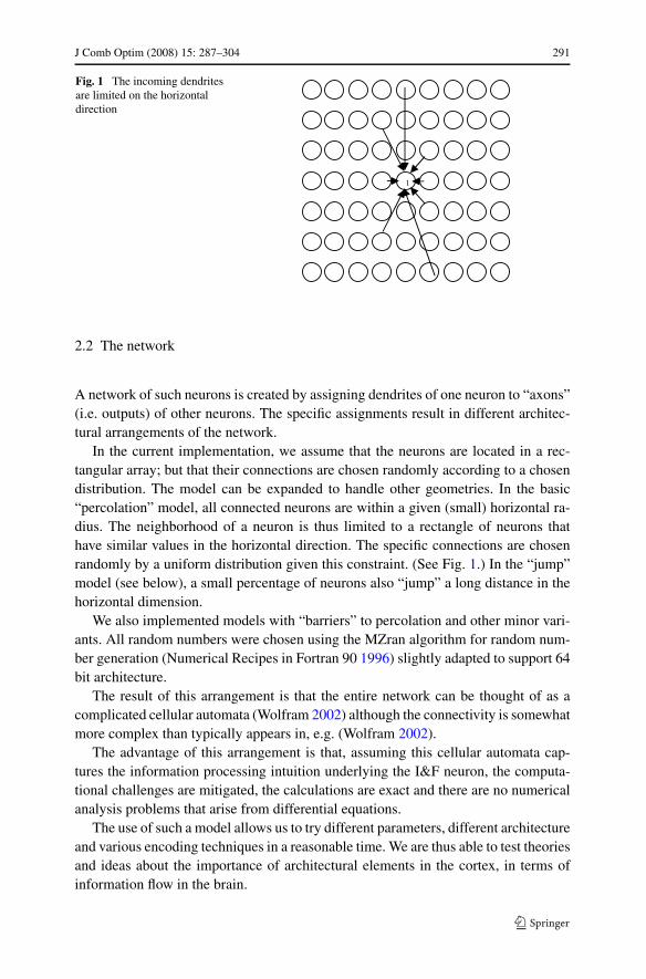
Fig. 1 The incoming dendritesare limited on the horizontaldirection

2.2 The network

A network of such neurons is created by assigning dendrites of one neuron to “axons”(i.e. outputs) of other neurons. The specific assignments result in different architec-tural arrangements of the network.

In the current implementation, we assume that the neurons are located in a rec-tangular array; but that their connections are chosen randomly according to a chosendistribution. The model can be expanded to handle other geometries. In the basic“percolation” model, all connected neurons are within a given (small) horizontal ra-dius. The neighborhood of a neuron is thus limited to a rectangle of neurons thathave similar values in the horizontal direction. The specific connections are chosenrandomly by a uniform distribution given this constraint. (See Fig. 1.) In the “jump”model (see below), a small percentage of neurons also “jump” a long distance in thehorizontal dimension.

We also implemented models with “barriers” to percolation and other minor vari-ants. All random numbers were chosen using the MZran algorithm for random num-ber generation (Numerical Recipes in Fortran 90 1996) slightly adapted to support 64bit architecture.

The result of this arrangement is that the entire network can be thought of as acomplicated cellular automata (Wolfram 2002) although the connectivity is somewhatmore complex than typically appears in, e.g. (Wolfram 2002).

The advantage of this arrangement is that, assuming this cellular automata cap-tures the information processing intuition underlying the I&F neuron, the computa-tional challenges are mitigated, the calculations are exact and there are no numericalanalysis problems that arise from differential equations.

The use of such a model allows us to try different parameters, different architectureand various encoding techniques in a reasonable time. We are thus able to test theoriesand ideas about the importance of architectural elements in the cortex, in terms ofinformation flow in the brain.

292 J Comb Optim (2008) 15: 287–304

3 Information theory methods

Assuming the use of such neurons in a large model, the next step is analyzing theresults of such large networks. In our work, we have implemented a tool that tracksthe mutual information. This tool works according to the method that was describedin Rolls et al. (2003), and was based on the approach taken by Panzeri et al. (1999);Rolls and Deco (2002). The main details and insights from this reference are pre-sented below.

There are some reservations in the literature about the quality and applicabilityof this method in some circumstances; The mean number of spikes in the consid-ered time window should be small (Panzeri et al. 1999; Bezzi et al. 2002). However,our testing, indicates that this method is reliable for our purposes. More specifically,Panzeri et al. (1999) indicates that tracking many neurons reduces the period of timethe formulas remain accurate. Panzeri et al. (1999) showed that one can use the for-mulas on about 10–15 neurons for the time periods of interest. Accordingly, althoughwe track 50 neurons, we used the formulas for subsets of 7 neurons and reported theaverage of ten such sets. This is described in Sect. 5.

Information theory measures provide a way to estimate how many stimuli couldbe encoded as a function of the responses. For a neuronal population C and a dis-crete set of stimuli S, a neuronal response n for each stimulus is defined as a vectorconsisting of the number of spikes emitted by each cell during a time window t . Therate response r is the vector n divided by t . ri , ni refer to the value at the ith loca-tion. A trial is a simulation of the ensemble for a specific stimulus. Multiple trials areperformed for each stimulus.

The response set R consists of all the responses for all the stimuli of S in all thetrials. The Shannon mutual information formula evaluates how much information isshared between S and R. Alternatively, it can be viewed as the amount of informationthat was captured in the responses. The formula uses the probabilities of S and R andthe joint probability P(S,R).

I (t) =∑

s∈S

∑

r

P (s, r) log2P(s, r)

P (s)P (r). (1)

To use this formula empirically, sufficient trials are needed to estimate the correctprobabilities. Unfortunately, even for a few cells, there can not be enough samples.This causes various difficulties including biased probabilities calculation, see Panzeriet al. (1999). Moreover, the sampling error increases exponentially with the numberof spikes. That is, with more spikes comes more options for responses, and thus, moretrials are needed to assess the probability for each response.

Panzeri et al. (1999) tackled this under-sampling problem by making a Taylor se-ries approximation. Taylor series is adequate for calculating the function value insmall neighborhoods. They calculate I (t), the mutual information (MI) for time in-terval t around 0, using only the first two time derivatives It and Itt . The refractoryperiod limits the number of emitted spikes. Thus, in a small windows, the expectedvalues of n are usually 0–2 spikes. According to Rolls et al. (2003) the approximationby using the Taylor series up to the second derivatives is accurate in this range whereeach neuron fires 1–2 spikes. (Note that, for our purposes, I (0) is 0, and higher deriv-atives are negligible in a small population with such small values.) This short time

J Comb Optim (2008) 15: 287–304 293

limitation is reasonable since the relevant sensory information is transmitted in a shorttime (Rolls et al. 2003). Hence the mutual information I (t) available is calculated by

I (t) = t (It ) + t2

2(Itt ). (2)

Following Rolls et al. (2003) (and using their notation), the instantaneous mutualinformation rate It is a summation of the instantaneous information rate of each singlecell from ensemble C cells. The 〈 〉s stands for an average across stimuli.

It =C∑

i=1

⟨

ri(s) log2ri(s)

〈ri(s′)〉s′

⟩

s

. (3)

This term evaluates how the average of the responses (across trials) of a cell aresimilar to his mean response across stimuli.

The second time derivative of the information accounts for the pairwise correla-tions. The expression for the second time derivative of the mutual information Itt

breaks up into three terms: Itta, Ittb and Ittc. According to Rolls et al. (2003), Ittais a negative value which reduces the amount of redundancy produced by concurrentfirings. The second term, Ittb, adds the actual information that results from the corre-lation i.e. synergy. The last term, Ittc, stands for stimulus dependent correlations.

Itt = Itta + Ittb + Ittc, (4)

Itta = 1

ln 2

C∑

i=1

C∑

j=1

〈ri(s)〉s〈rj (s)〉s[

νij + (1 + νij ) ln1

1 + νij

]

, (5)

Ittb =C∑

i=1

C∑

j=1

[〈ri(s)rj (s)γij (s)〉s] log21

1 + νij

, (6)

Ittc =C∑

i=1

C∑

j=1

⟨

ri(s)rj (s)(1 + γij (s)) log2

[(1 + γij (s))〈ri(s

′)rj (s′)〉′s

〈ri(s′)rj (s′)(1 + γij (s′))〉′s

]⟩

s

. (7)

The shuffling method (Rolls et al. 2003) for estimating the Ittc validity was imple-mented as well. The Monte Carlo procedure mainly consists of reevaluating the termfor the data when the trials are shuffled within a stimulus. The “confidence limit” waskept as 2 std from the average.

The above formulas are defined in terms of two types of correlations:

γij (s) = ni(s)nj (s)

ni(s)nj (s)− 1, (8)

γii(s) = ni(s)nj (s) − ni(s)

ni(s)nj (s)− 1, (9)

294 J Comb Optim (2008) 15: 287–304

νij = 〈ni(s)nj (s)〉s〈ni(s)〉s〈nj (s)〉s − 1 = 〈ri(s)rj (s)〉s

〈ri(s)〉s〈rj (s)〉s − 1. (10)

The mutual information (MI) formulas uses only the spike counts to express theamount of synergy and redundancy of the introduced correlations. Thus, the compu-tations are done relative to a discrete set of stimuli and a set of possible responses,aka trial results, for each stimuli. This relative nature of the measure is useful whencomparing different networks. The result of these formulas describes how many bitsof information are present in each architecture.

The different components of the formulas relate to the encoding methods. The twomain ways to encode information are (a) the firing rates and the spikes counts and(b) the correlations. Correlations occur when the firings of neurons are related foronly some of the stimuli. For example, if the firing of two cells is concurrent for onlyone of the stimuli, it would be easier to know which stimulus was applied. One cansee that in MI terms, this increases the ability to discriminate between the stimuli.The different parts of the formulas I (t) correspond to different kind of encodings(Rolls et al. 2003). This is very advantageous when we compare architectures. Thus,the formulas allow us to understand how different encoding methods are affected indifferent architectures as well as the rate and the flow of information in the brainthrough time.

Since the formulas require a distribution, hundreds of trials are needed for eachstimulus in each test. Due to this time consuming limitation, most of the experimentsin this paper are demonstrated for neuronal populations of about 10,000. This exhibitsthe same behavior as the populations of 100,000 which we tried as well. To be clear,the limitation in computation time is due to the information theoretic requirements,not to the simulation of the neurons themselves.

The different trials are produced in our tool by the addition of Gaussian noise.Without noise, the trials would be identical for each stimulus, and no distributionwould be produced. To compute the correct probability, enough trials are required tocover all the possibilities that occur. To verify that the sampling error is decreasingwe checked the information for varying numbers of trials. This gives some estimationon the decrement of the error. Since additional trials produces a more exact distribu-tion, this can be used to give an indication of the variation on an individual trial; i.e.how robust a system is to the addition of noise. In other words, the number of trialsneeded to give a reliable estimate of mutual information gives an indication of thevariance in the results of computation under noise which thus indicates how reliablethe system is. The methodology is described in Sect. 5 where it is used to show thatsome architectures may be more reliable than others.

As explained above, the formula is valid for short time intervals. In addition, whenmore cells are checked and higher number of spikes are produced the time validity isreduced even further (Panzeri et al. 1999; Bezzi et al. 2002). Previous tests (Rolls etal. 2003) were done for fewer cells. In the tests below, we checked the informationfor 50 representative neurons. To overcome this obstacle, we computed the infor-mation 10 times, for different randomly selected 7 neurons, out of the 50. The totalinformation reported is the average of all the groups of 7 representatives. The num-ber of groups and selected neurons can be determined as external parameters in theimplemented system.

J Comb Optim (2008) 15: 287–304 295

4 Tool capacity and capability

Two software modules were developed, the simulator and the information compo-nent.

The simulator is an implementation of the model, which produces a spike train his-tory of a selected subset of neurons. The usual procedure chooses neurons randomly,from specific locations, or by other criteria. In the runs discussed in this paper, thenumber of selected neurons was usually set to 50.

The spike train of these neurons is then used for further analysis by the informationmodule. The spike train history is also saved and is available for further analysis.The simulator, in its current implementation, allows trials to be run in parallel, butthe neurons are processed sequentially. However, the essential mechanism is wellsuited to future parallization, and this was kept in mind during the design of the datastructures. The program is implemented in the programming language C. The currentexperiments used a 64-bit machine with dual processors and 16 Gigabytes of memory.This is sufficient to, in principle, simulate up to 50 million neurons with a fan in ofabout 21.

The choice of topology is flexible, allowing the potential implementation of rel-atively realistic anatomy. The connectivity of the neurons can be chosen either ran-domly or specifically. In addition, it is easy to implement specific constraints, e.g.that connectivity is within a certain radius of a neuron.

There are many different external parameters that can be assigned, such as decayrate, leak rate, threshold, refractory period, size of connectivity fan-in and the num-ber of neurons whose spike history will be recorded. The design of the simulator isby simple building blocks, so that new knowledge and requirements can be easilyincorporated into the program.

In addition, the size of the time discretization is a parameter; both the total numberof seconds and the number of parts in a second.

There is also the option of adding an external input to the neurons. This can betuned by setting the time and location at which the external input will be applied.

An efficient algorithm (Numerical Recipes in Fortran 90 1996), modified to sup-port 64-bit architecture machines, for random number generator is used; this is crucialbecause of the huge number of random numbers needed. The random generator seedscan also be changed.

Information theoretic techniques as described in the previous section were im-plemented in MATLAB. This requires multiple trials for each stimulus. Variation inthe responses is obtained by the addition of a noise factor, generated by a Gaussiandistribution, that is added to the potential of the neurons. The polarity of the noise(inhibitory, excitatory) is an external parameter. Other parameters of the noise (e.g.distribution parameters) are also external parameters.

In the tests reported in this paper, we simulated 100 trials for each stimulus. Forcomparison, in Rolls et al. (2003) 20 trials for 8 cells were run. We used the method-ology described below in Sect. 3, to verify that 100 trials suffice.

Our machine has 16 gigabyte memory with a 2.4 gigahertz processor. This allowsus to store as many as 50M neurons with 21 inputs to each one, which can be thoughtof as a bi-dimensional piece of cortex of 1000 × 50,000. The largest model we have

296 J Comb Optim (2008) 15: 287–304

actually run is 1M neurons with 21 inputs. Thus a run of 3000 logical time stepscorresponds to simulating 3 seconds in the real biological world.

Under our implementation it takes about 1500 seconds to simulate 1 trial on theaverage (across stimuli and trials) for 1M neurons. A simulation of one trial for 104

neurons takes 1.84 seconds and 2×104 neurons takes 4.4 seconds. In each of our testswe used 21 inputs for each neuron. This number is chosen according to the proportionof neurons and connections as in Marom and Shahaf (2002). The complexity upperbound is linear on the number of connections and inputs as can be deduced from theabove model. The actual running time depends on the total neurons and connectivityas well as processes memory.

5 Experiments and results

Having developed the simulator and information tools; we ran the following classesof experiments:

(i) Preliminary experiments. These show that the results themselves are consistentwith the literature and that simple changes in parameters are in consonance withcommon intuition.

We reran the tests with different parameters, e.g. different size networks, providinga way to assess the inner consistency of new results. The parameters were varied forthe topology and number of neurons, connectivity, integrate and fire parameters andtime parameters. We ran the tests on different stimuli, different discretization timebins, and we chose different locations for applying the stimulus or checking the MI.

We tested the network with parameters that seem common in the literature (Panzeriet al. 1999; Schüz 1998): total time simulation of about 100 ms; time discretizationslices of about 1 ms; and refractory periods of 2 ms. The choice of fan-in; i.e. numberof “dendrites” to the neuron was chosen as 21. Non-determinism in the network isestablished by adding noise parameters to the neuronal responses. The most basicnetworks were rectangular with local connectivity (i.e. neurons could only connect toother neurons within a certain horizontal distance). See Fig. 1.

For example, we tested whether the approximation of the mutual information asgiven by formula (2), is valid for the consequences of sending no information to thenetwork. No information is transmitted when there is no difference in response as thestimulus is varied, even if there is a distribution of response for a given stimulus. Thiswas done in different ways, e.g., by using an architecture with a “barrier” betweenthe stimulus and response. In this case, the formulas do in fact result in extremelysmall mutual information as anticipated.

(ii) Experiments testing the relationship of connectivity to the rate of growth ofmutual information and to the total amount of mutual information.

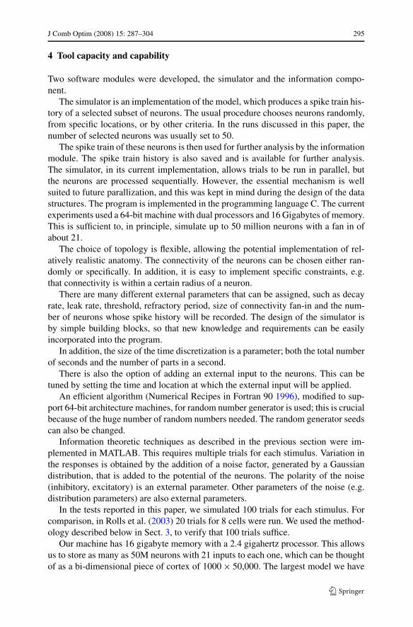
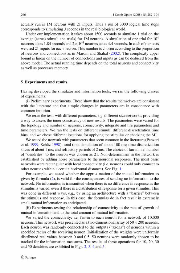
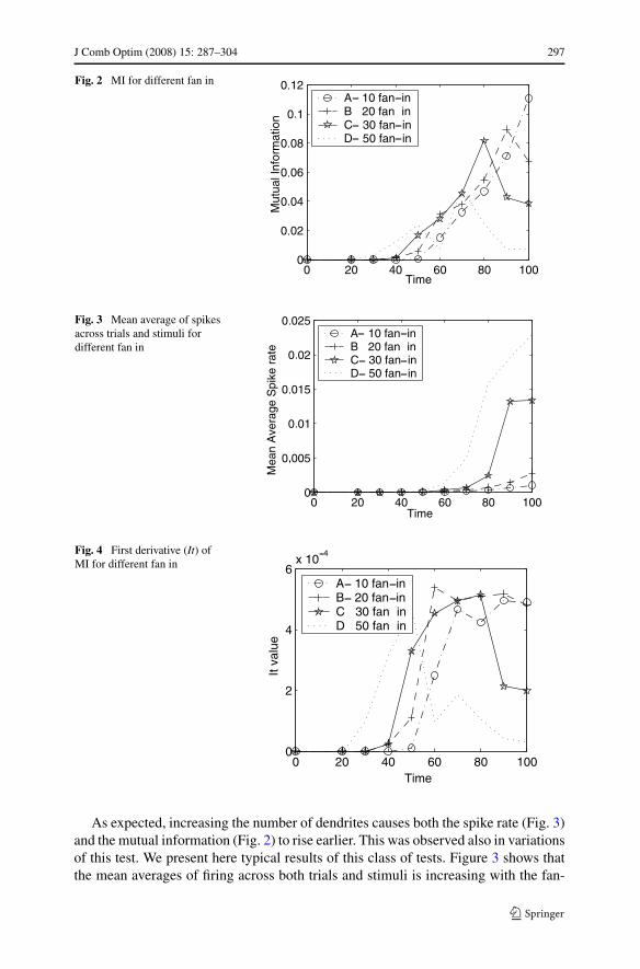
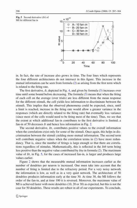
We varied the connectivity; i.e. fan-in to each neuron for a network of 10,000neurons. This network was presented as a two-dimensional array of 50×200 neurons.Each neuron was randomly connected to the outputs (“axons”) of neurons within aspecified radius of the receiving neuron. Initialization of the weights were uniformlydistributed real values between 0 and 0.5. 50 neurons were randomly chosen to betracked for the information measures. The results of these operations for 10, 20, 30and 50 dendrites are exhibited in Figs. 2, 3, 4 and 5.

J Comb Optim (2008) 15: 287–304 297

Fig. 2 MI for different fan in

Fig. 3 Mean average of spikesacross trials and stimuli fordifferent fan in

Fig. 4 First derivative (It) ofMI for different fan in

As expected, increasing the number of dendrites causes both the spike rate (Fig. 3)and the mutual information (Fig. 2) to rise earlier. This was observed also in variationsof this test. We present here typical results of this class of tests. Figure 3 shows thatthe mean averages of firing across both trials and stimuli is increasing with the fan-

298 J Comb Optim (2008) 15: 287–304

Fig. 5 Second derivative (Itt) ofMI for different fan in

in. In fact, the rate of increase also grows in time. The four lines which representsthe four different architectures do not intersect in this figure. This increase in themutual information can be seen from formula (2) as arising from the first term whichis related to the firing rate.

The first derivative, It, depicted in Fig. 4, and given by formula (3) increases overtime until some bound before decreasing. The formula (3) means that when the firingof each cell on the average (over trials) are less different from the mean responsefor the different stimuli, the cell yields less information to discriminate between thestimuli. This implies that the observed phenomena could be expected, since, untila limit is reached, increase in the firing rate would allow a greater variance in theresponses (which are directly related to the firing rate) but eventually less variance(since most of the cells would need to be firing most of the time). Thus, we see thatthe extent at which additional fan-in contributes to the first derivative is limited; afan-in of 50 decreases It and hence less information in Fig. 2.

The second derivative, Itt, contributes positive values to the overall informationwhen the correlations exist only for some of the stimuli. Once again, this helps in dis-crimination between the stimuli yielding more mutual information. The second termwill contribute negative values when the correlation terms in (2) have more redun-dancy. That is, since the number of firings is large enough so that there are correla-tions regardless of stimulus. Mathematically, this is reflected in the Ittb term beingless positive than the negative value contributed by Itta in formula (2). The maximumvalue of Itt, in Fig. 5, for the cases of increased fan-in, is larger and produces largevalues earlier.

Figure 2 shows that the measurable mutual information increases earlier as thenumber of dendrites per neuron is increased. One must take into account that thenumber of firing is limited due to the refractory period. For a very noisy networkthe information is low, as well as in a very quiet network. The architecture of 50dendrites produces information early at the time 30. At time 30, the MI follows theorder of the fan-in, and at time 100 it is reversed. Moreover, the maximum value ofMI is achieved faster with more dendrites (10, 20 or 30) as expected, but this is not thecase for 50 dendrites. These results are robust in all of our experiments. To conclude,

J Comb Optim (2008) 15: 287–304 299

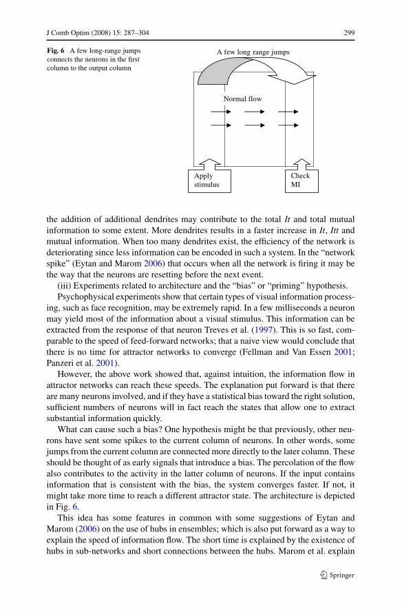
Fig. 6 A few long-range jumpsconnects the neurons in the firstcolumn to the output column

the addition of additional dendrites may contribute to the total It and total mutualinformation to some extent. More dendrites results in a faster increase in It, Itt andmutual information. When too many dendrites exist, the efficiency of the network isdeteriorating since less information can be encoded in such a system. In the “networkspike” (Eytan and Marom 2006) that occurs when all the network is firing it may bethe way that the neurons are resetting before the next event.

(iii) Experiments related to architecture and the “bias” or “priming” hypothesis.Psychophysical experiments show that certain types of visual information process-

ing, such as face recognition, may be extremely rapid. In a few milliseconds a neuronmay yield most of the information about a visual stimulus. This information can beextracted from the response of that neuron Treves et al. (1997). This is so fast, com-parable to the speed of feed-forward networks; that a naive view would conclude thatthere is no time for attractor networks to converge (Fellman and Van Essen 2001;Panzeri et al. 2001).

However, the above work showed that, against intuition, the information flow inattractor networks can reach these speeds. The explanation put forward is that thereare many neurons involved, and if they have a statistical bias toward the right solution,sufficient numbers of neurons will in fact reach the states that allow one to extractsubstantial information quickly.

What can cause such a bias? One hypothesis might be that previously, other neu-rons have sent some spikes to the current column of neurons. In other words, somejumps from the current column are connected more directly to the later column. Theseshould be thought of as early signals that introduce a bias. The percolation of the flowalso contributes to the activity in the latter column of neurons. If the input containsinformation that is consistent with the bias, the system converges faster. If not, itmight take more time to reach a different attractor state. The architecture is depictedin Fig. 6.

This idea has some features in common with some suggestions of Eytan andMarom (2006) on the use of hubs in ensembles; which is also put forward as a way toexplain the speed of information flow. The short time is explained by the existence ofhubs in sub-networks and short connections between the hubs. Marom et al. explain

300 J Comb Optim (2008) 15: 287–304

Fig. 7 MI of the “jumparchitecture”

Fig. 8 Mean average of spikesacross trials and stimuli of the“jump architecture”

the short time by larger connectivity, in our case the short time is produced by thejumps.

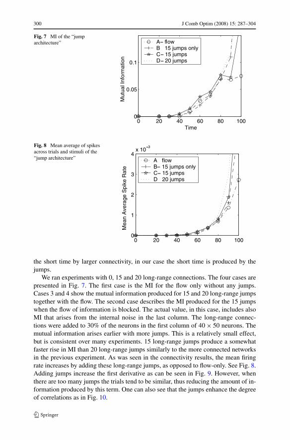
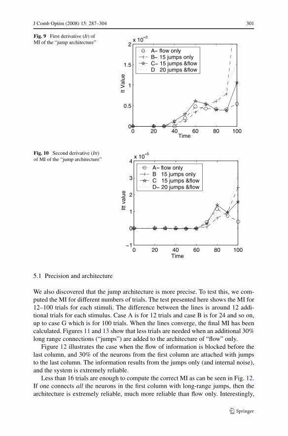
We ran experiments with 0, 15 and 20 long-range connections. The four cases arepresented in Fig. 7. The first case is the MI for the flow only without any jumps.Cases 3 and 4 show the mutual information produced for 15 and 20 long-range jumpstogether with the flow. The second case describes the MI produced for the 15 jumpswhen the flow of information is blocked. The actual value, in this case, includes alsoMI that arises from the internal noise in the last column. The long-range connec-tions were added to 30% of the neurons in the first column of 40 × 50 neurons. Themutual information arises earlier with more jumps. This is a relatively small effect,but is consistent over many experiments. 15 long-range jumps produce a somewhatfaster rise in MI than 20 long-range jumps similarly to the more connected networksin the previous experiment. As was seen in the connectivity results, the mean firingrate increases by adding these long-range jumps, as opposed to flow-only. See Fig. 8.Adding jumps increase the first derivative as can be seen in Fig. 9. However, whenthere are too many jumps the trials tend to be similar, thus reducing the amount of in-formation produced by this term. One can also see that the jumps enhance the degreeof correlations as in Fig. 10.

J Comb Optim (2008) 15: 287–304 301

Fig. 9 First derivative (It) ofMI of the “jump architecture”

Fig. 10 Second derivative (Itt)of MI of the “jump architecture”

5.1 Precision and architecture

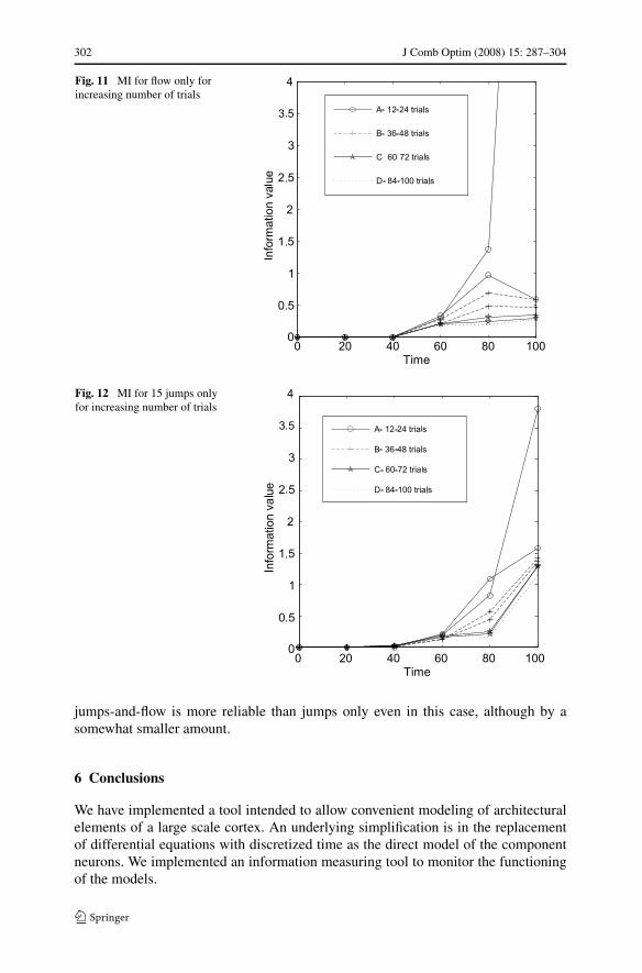
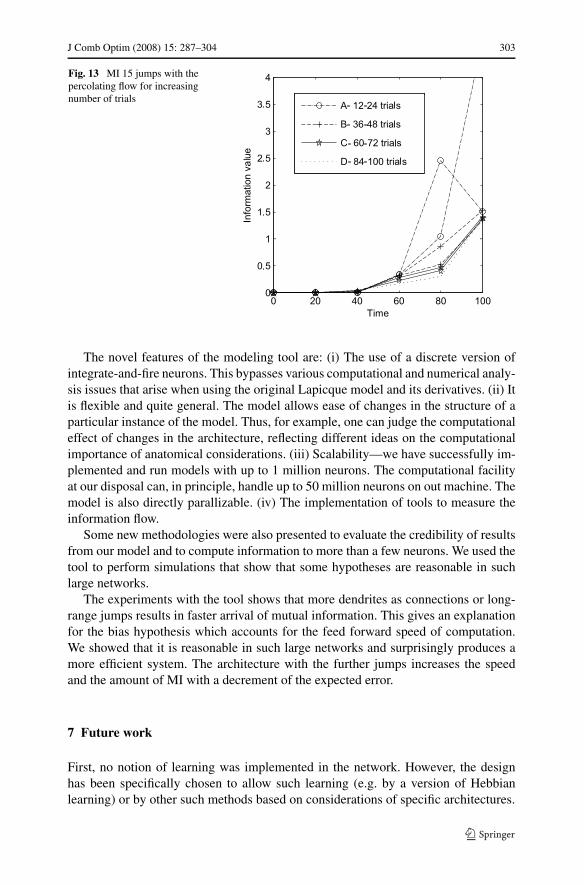
We also discovered that the jump architecture is more precise. To test this, we com-puted the MI for different numbers of trials. The test presented here shows the MI for12–100 trials for each stimuli. The difference between the lines is around 12 addi-tional trials for each stimulus. Case A is for 12 trials and case B is for 24 and so on,up to case G which is for 100 trials. When the lines converge, the final MI has beencalculated. Figures 11 and 13 show that less trials are needed when an additional 30%long range connections (“jumps”) are added to the architecture of “flow” only.

Figure 12 illustrates the case when the flow of information is blocked before thelast column, and 30% of the neurons from the first column are attached with jumpsto the last column. The information results from the jumps only (and internal noise),and the system is extremely reliable.

Less than 16 trials are enough to compute the correct MI as can be seen in Fig. 12.If one connects all the neurons in the first column with long-range jumps, then thearchitecture is extremely reliable, much more reliable than flow only. Interestingly,

302 J Comb Optim (2008) 15: 287–304

Fig. 11 MI for flow only forincreasing number of trials

Fig. 12 MI for 15 jumps onlyfor increasing number of trials

jumps-and-flow is more reliable than jumps only even in this case, although by asomewhat smaller amount.

6 Conclusions

We have implemented a tool intended to allow convenient modeling of architecturalelements of a large scale cortex. An underlying simplification is in the replacementof differential equations with discretized time as the direct model of the componentneurons. We implemented an information measuring tool to monitor the functioningof the models.

J Comb Optim (2008) 15: 287–304 303

Fig. 13 MI 15 jumps with thepercolating flow for increasingnumber of trials

The novel features of the modeling tool are: (i) The use of a discrete version ofintegrate-and-fire neurons. This bypasses various computational and numerical analy-sis issues that arise when using the original Lapicque model and its derivatives. (ii) Itis flexible and quite general. The model allows ease of changes in the structure of aparticular instance of the model. Thus, for example, one can judge the computationaleffect of changes in the architecture, reflecting different ideas on the computationalimportance of anatomical considerations. (iii) Scalability—we have successfully im-plemented and run models with up to 1 million neurons. The computational facilityat our disposal can, in principle, handle up to 50 million neurons on out machine. Themodel is also directly parallizable. (iv) The implementation of tools to measure theinformation flow.

Some new methodologies were also presented to evaluate the credibility of resultsfrom our model and to compute information to more than a few neurons. We used thetool to perform simulations that show that some hypotheses are reasonable in suchlarge networks.

The experiments with the tool shows that more dendrites as connections or long-range jumps results in faster arrival of mutual information. This gives an explanationfor the bias hypothesis which accounts for the feed forward speed of computation.We showed that it is reasonable in such large networks and surprisingly produces amore efficient system. The architecture with the further jumps increases the speedand the amount of MI with a decrement of the expected error.

7 Future work

First, no notion of learning was implemented in the network. However, the designhas been specifically chosen to allow such learning (e.g. by a version of Hebbianlearning) or by other such methods based on considerations of specific architectures.

304 J Comb Optim (2008) 15: 287–304

Second, it is natural to consider sequences of such networks linked and reactingto the early “guesses” we have isolated, and to verify that successful computationalprocessing can be carried out by such guesses.

Third, the advantage of additional jumps and dendrites is confined to a limitedamount of MI, speed and accuracy of computation. The amount of such jumps thusdepends on the number of neurons, connectivity and the internal features of suchneurons. One may try to assess the optimal jump structure for an architecture.

The tool is now ready for use in more physiologically specific architectures.

Acknowledgements This work was conceived when LM was on a sabbatical visit to Edmund Rollslaboratory in Oxford, UK; and an early version of the simulator was written there. LM thanks Prof. Rollsfor his hospitality. Leonardo Franco is particularly thanked for explicating the use of information theoryin this context and Paul Gabbott is thanked for painstakingly describing various aspects of physiology.This work is part of the M.Sc. thesis of MM at the U. Haifa where she was supported by the CaesareaRothschild Center and the Neurocomputation Laboratory. MM thanks them, and LM for his guidance.

References

Abbott LF (1999) Lapicque’s introduction of the integrate-and-fire model neuron (1907). Brain Res Bull50:303–304

Bezzi M, Diamond ME, Treves A (2002) Redundancy and synergy arising from pairwise correlations inneuronal ensembles. J Comp Neurosci 12:165–174

Braitenberg V, Schüz A (1998) Cortex: statistics and geometry of neuronal connectivity. Springer, Berlin(Revised edition of Anatomy of the cortex, statistics and geometry, 1991)

Eytan D, Marom S (2006) The network spike: a basic mode of synchronization within and between neu-ronal assemblies. PhD thesis, Faculty of Medicine, Technion

Fellman DJ, Van Essen DC (2001) Distributed hierarchical processing in the primate visual cortex. CerebCortex 1:1–47

Hodgkin AL, Huxley AF (1952) A quantitative description of membrane current and its application toconduction and excitation in nerve. J Physiol 117:500–544

Lapicque L (1907) Recherches quantitatives sur l’excitation lectrique des nerfs traite comme une polarisa-tion. Physiol Pathol Gen 9:620–635

Marom S, Shahaf G (2002) Development, learning and memory in large random networks of corticalneurons:lesson beyond anatomy. Q Rev Biophys 35:63–87

Numerical recipes in Fortran 90 (1996) The art of scientific parallel computing, scientific computing.Cambridge University Press, Cambridge

Panzeri S, Schultz SR, Treves A, Rolls ET (1999) Correlations and encoding of information in the nervoussystem. Proc R Soc Lond Ser B: Biol Sci 266:1001–1012

Panzeri S, Rolls ET, Battaglia F, Lavis R (2001) Speed of feed forward and recurrent processing in multi-layer networks of integrate-and-fire neurons. Network 12(4):423–440

Rolls ET, Deco G (2002) Computational neuroscience of vision. Oxford University Press, OxfordRolls ET, Franco L, Aggelpoulos NC, Reece S (2003) An information theoretic approach to the contribu-

tions of the firing rates and the correlations between the firing of neurons. Neurophysiol 89:2810–2822

Schüz A (1998) Neuroanatomy in a computational perspective. In: Arbib MA (ed) Handbook of braintheory and neural networks. MIT Press, Cambridge

The genesis simulator (1994–2006) http://www.genesis-sim.org/GENESISTrappenberg TP (2002) Fundamental of Computational Neuroscience. Oxford University Press, OxfordTreves A, Rolls ET, Simmen M (1997) Time for retrieval in recurrent associative memories. Physica D

107:392–400Wolfram S (2002) A new kind of science. Wolfram Media, Inc