


Bahasa
Halaman
Hukum


A Note On the Bounds for the Generalized Fibonacci-p-Sequence and
its Application in Data-Hiding
Sandipan Dey
Microsoft India Development [email protected]
Hameed Al-QaheriDepartment of Quantitative Methods and Information Systems
College of Business Administration
Kuwait [email protected]
Suneeta SaneComputer and Information Technology Department
Veermata Jijabai Technological Institute
Mumbai, Maharashtra 400019, [email protected]
Sugata SanyalSchool of Technology and Computer Science
Tata Institute of Fundamental Research
Homi Bhabha Road, Mumbai - 400005, [email protected]
July 2008
In this paper, we suggest a lower and an upper bound for the Generalized Fibonacci-
p-Sequence, for different values of p. The Fibonacci-p-Sequence is a generalization of the
Classical Fibonacci Sequence. We first show that the ratio of two consecutive terms ingeneralized Fibonacci sequence converges to a p-degree polynomial and then use this re-
sult to prove the bounds for generalized Fibonacci-p sequence, thereby generalizing the
exponential bounds for classical Fibonacci Sequence. Then we show how these resultscan be used to prove efficiency for data hiding techniques using generalized Fibonacci
sequence. These steganographic techniques use generalized Fibonacci-p-Sequence for in-creasing the number of available bit-planes to hide data, so that more and more datacan be hidden into the higher bit-planes of any pixel without causing much distortion
of the cover image. This bound can be used as a theoretical proof for efficiency of those
techniques, for instance it explains why more and more data can be hidden into thehigher bit-planes of a pixel, without causing considerable decrease in PSNR.
Keywords: Fibonacci-sequence, LSB Data-hiding, PSNR
1. Introduction
Among many different data hiding techniques proposed to embed secret message
within images, the LSB data hiding technique is one of the simplest methods for
inserting data into digital signals in noise free environments, which merely embeds
secret message-bits in a subset of the LSB planes of the image. (LSB is the least
significant bit or the 0th bit, the second LSB is the 1st bit, and so on). Despite
1
arX
iv:1
005.
1953
v2 [
cs.C
R]
13
Oct
201
0

2 Dey, Al-Qaheri, Sane, Sanyal
being simple, this technique is more predictable and hence less secure, also PSNR
(peak signal to noise ratio) decreases very rapidly as we use the higher bit planes
for data hiding. As soon as we go from LSB (least significant bit) to MSB (most
significant bit) for selection of bit-planes for our message embedding, the distortion
in stego-image is likely to increase exponentially, so it becomes impossible (without
noticeable distortion and with exponentially increasing distance from cover-image
and stego-image) to use higher bit-planes for embedding without any further pro-
cessing. The workarounds may be: through the random LSB replacement (in stead
of sequential), secret messages can be randomly scattered in stego-images, so the
security can be improved. Also, using the approaches given by variable depth LSB
algorithm [Liu et al. (2004)], or by the optimal substitution process based on genetic
algorithm and local pixel adjustment [Wang et al. (2001)], one is able to hide data
to some extent in higher bit-planes as well.
Battisti et al. [Battisti et al. (2006)], [Picione et al. (2006)] proposed a novel
data hiding technique from a totally different perspective, it uses a different bit-
planes decomposition altogether, based on the generalized Fibonacci-p-sequences,
that not only increases the number of embeddable bit-planes but also decreases
PSNR in the stego image considerably, thereby improving the LSB technique. In
this paper, we first prove some theoretical upper and lower bounds for generalized
Fibonacci-p-sequence and give a theoretical proof for the better performance of the
data hiding technique using generalized Fibonacci decomposition, i.e., why the data
hiding technique using this decomposition not only gives larger number of bit planes
for hiding secret bits, but also gives a far better PSNR than that in classical LSB
technique.
The Generalized Fibonacci-p-Sequence ([Horadam (1961)], [Basin and Hoggatt
(1963)], [Hoggatt (1972)], [Atkins and Geist (1987)], [Hendel (1994)], [Sun and Sun
(1992)]) is given by,
Fp(0) = Fp(1) = . . . = Fp(p) = 1,
Fp(n) = Fp(n− 1) + Fp(n− p− 1), ∀n ≥ p+ 1, n, p ∈ N (1)
For p = 1, we have,
F (0) = F (1) = 1,
F (n) = F (n− 1) + F (n− 1), ∀n ≥ 2, n ∈ N
We get the classical Fibonacci sequence 1, 1, 2, 3, 5, 8, . . .. We already have some
results for this Classical Fibonacci Sequence, e.g., we know the ratio of two consec-
utive terms in Fibonacci sequence converge to Golden Ratio, 1+√5
2 . In this paper,
we show that αnp > Fp(n) > αn−pp , ∀n, p ∈ N, where αp is the positive Root of
xp+1 − xp − 1 = 0. The ratio of two consecutive terms in Fibonacci-p-Sequence
converges to this αp.

Bounds for the Generalized Fibonacci-p-Sequence and its Application in Data-Hiding 3
2. Bounds for the generalized Fibonacci-p-Sequence
In this section we prove the upper and lower bounds for the generalized Fibonacci-
p-sequence. First, we show that the ratio of consecutive terms of generalized
Fibonacci-p-sequence converges to the positive root of the polynomial xp+1−xp−1 =
0. Next we use this root to prove a bound on the generalized Fibonacci-p-sequence.
2.1. Lemma 1
The ratio of two consecutive numbers in generalized Fibonacci p-sequence converges
to the positive root of the degree-p polynomial P (x) = xp+1 − xp − 1.
Proof:
Convergence
Let us first define the ratio of two consecutive terms of Fibonacci-p-sequence as a
sequence {βn} ={Fp(n+1)Fp(n)
}.
Now, by definition of Fibonacci-p-sequence, we have
β0 = β1 = · · · = βp = 1
βn = 1 +Fp(n− p)Fp(n)
> 1, ∀n > p
βp+1 = βp + β0 = 1 + 1 = 2
βn = 1 +Fp(n− p)Fp(n)
< 1 + 1 = 2, ∀n > p+ 1
⇒ 1 < βn < 2, ∀n > p+ 1
We observe that the sequence βn is bounded and hence by Monotone Conver-
gence theorem must have a convergent subsequence. For instance, for p = 1 (classi-
cal Fibonacci sequence), we have two convergent subsequences β2n (increasing) and
β2n+1 (decreasing), n ∈ N (natural number) and they both converge to the same
limit 1+√5
2 ≈ 1.618 [Craw (2000)], as shown in figure 2.
Positive Root of the polynomial xp+1 − xp − 1
Now, let’s analyze the polynomial function y = P (x) = xp+1−xp−1. By Descartes’
rule, the polynomial can have at most one positive real root, since it has exactly
one change in sign.
First we observe that the function P (x) is continuous and differentiable every-
where. We also notice that the function has exactly one positive root αp (and αpis also strictly larger than 1). This is a consequence of elementary calculus. By
successive differentiation, we see that

4 Dey, Al-Qaheri, Sane, Sanyal
y1 = P ′(x) = (p+ 1)xp − pxp−1
y2 = P ′′(x) = (p+ 1)pxp−1 − p(p− 1)xp−2
• The function P (x) has critical points at P ′(x) = 0, i.e., at x = 0 and
x = pp+1 .
• y2∣∣∣x= p
p+1
= pp−1
(p+1)p−2 > 0, ∀p ≥ 1.
• By 2nd order sufficient condition for local minima, P (x) has a (local) min-
ima at x = pp+1 .
• At x = 0, the function will have a maxima or a point of inflection depending
on whether p is odd or even, explained in the next section.
When p ∈ Nodd, we have,
y1 = P ′(x) = (p+ 1)xp−1(x− p
p+1
)is
< 0 x < 0
= 0 x = 0
< 0 0 < x < pp+1
= 0 x = pp+1
> 0 x > pp+1
Hence the function is decreasing in(−∞, p
p+1
)and increasing in
(pp+1 ,∞
).
Also, y(−1) = 1, y(0) = y(1) = −1 and y(2) = 2p − 1 ≥ 1, ∀p ∈ Nodd. At x = pp+1 ,
P (x) has a minima (gradient changes from negative to positive) but at x = 0 (no
sign change in gradient) we have a point of inflection. Again, P (x) being a contin-
uous function assumes all possible values within an interval. Combining all these,
we can easily see that the graph of the function has exactly two real zeroes, one
positive and the other negative (the remaining roots are complex conjugate pairs).
When p ∈ Neven, we have,
y1 = P ′(x) = (p+ 1)xp−1(x− p
p+1
)is
> 0 x < 0
= 0 x = 0
< 0 0 < x < pp+1
= 0 x = pp+1
> 0 x > pp+1
Hence the function is increasing in (−∞, 0), then decreasing in
(0, p
p+1
)and
again increasing in(
pp+1 ,∞
). Also, y(−1) = y(0) = y(1) = −1 and y(2) = 2p−1 ≥
1, ∀p ∈ Neven. At x0 = pp+1 , P (x) has a minima but at x = 0 (gradient changes from
positive to negative) we have a maxima. Combining all these, we can easily see that
we have exactly one real (positive) root at αp, since y(1) < 0 and y(2) > 0, also y(x)
being continuous. (From this result we immediately have Lemma 2). From figure 1
we can see the graph of the degree-p polynomial, for odd and even p respectively.

Bounds for the Generalized Fibonacci-p-Sequence and its Application in Data-Hiding 5
Convergence to the positive root of the polynomial
Now, we show that if sequence {βn} converges to β, then β = αp.
Let’s assume the sequence {βn} converges to β ∈ <+. Now we prove, the se-
quence must converge to the only positive root αp of the above-stated p-degree
polynomial. By assumption,
β = limn→∞
(fn+pfn+p−1
)= limn→∞
(fn+p−1fn
)= . . . = lim
n→∞
(fnfn−1
)= . . . ,
fn = nth number in the F ibonacci− p Sequence, fn+p = fn+p−1 + fn−1
⇒ β = limn→∞
(fn+p−1 + fn−1
fn+p−1
)= limn→∞
(fnfn−1
),
⇒ β = 1 + limn→∞
k=n+p−2∏k=n−1
(fkfk+1
)= limn→∞
(fnfn−1
)
⇒ β = 1 +
k=p∏k=1
(1
β
)⇒ β = 1 +
1
βp
⇒ βp+1 − βp − 1 = 0
Hence β satisfies the equation xp+1 − xp − 1 = 0, ∀p ∈ N, β ∈ <+, i.e., from
above results, we have, β = αp
Fig. 1. Graph of xp+1 − xp − 1 = 0, showing αp for different values of p

6 Dey, Al-Qaheri, Sane, Sanyal
2.2. Lemma 2
If αp be a positive root of the equation xp+1 − xp − 1 = 0, we have 1 < αp < 2,
∀p ∈ N.
Proof: We have,
αp+1p − αpp − 1 = 0
Also, 2p+1 − 2p − 1 = 2p − 1 > 0, ∀p ∈ N⇒ 2p − 1 > αp+1
p − αpp − 1
⇒ (2p − αpp) > αpp(αp − 2) (2)
Also,
− 1 < 0 = αp+1p − αpp − 1
⇒ αpp(αp − 1) > 0
⇒ αp > 1 (since positive) (3)
From (2), we immediately see the following:
• αp > 0 according to our assumption, hence we can not have αp = 2 (LHS
& RHS both becomes 0, that does not satisfy inequality (2)).
• If αp > 2, we have LHS < 0 while RHS > 0 which again does not satisfy
inequality (2).
• Hence we have αp < 2, ∀p ∈ N
From (3), we have, αp > 1. Combining, we get, 1 < αp < 2, ∀p ∈ N
2.3. Lemma 3
If αp be a positive root of the equation xp+1 − xp − 1 = 0, where p ∈ N, we have
the following results, ∀k ∈ N,
• αk > αk+1
• limk→∞ αk = 1
• αk+1 >1+αk
2
• αkk < (k + 1)
• αk+1k > 1
Proof: We have,
For p = k, αk+1k − αkk − 1 = 0
For p = k + 1, αk+2k+1 − α
k+1k+1 − 1 = 0
⇒ αk+1k+1(αk+1 − 1) = αkk(αk − 1)
⇒(
αkαk+1
)k=
(αk+1 − 1
αk − 1
).αk+1 (4)

Bounds for the Generalized Fibonacci-p-Sequence and its Application in Data-Hiding 7
From (4) we can argue,
• αk 6= αk+1, since neither of them is 0 or 1 (from Lemma 2).
• If αk < αk+1, we have LHS of inequality (4) < 1, but RHS > 1, since both
the terms in RHS will be greater than 1 (by our assumption and by Lemma
2), a contradiction.
• Hence we must have
αk > αk+1, ∀k ∈ N (5)
Also, from Lemma 2, we have, 1 < αk < 2, ∀k ∈ N.
Hence we have,
2 > α1 > α2 > . . . > αk > αk+1 > . . . > 1, k ∈ N⇒ lim
k→∞αk = 1
Again, from (4) we have,
⇒(αk+1 − 1
αk − 1
).αk+1 > 1, since
(αkαk+1
)k> 1, from (5)
⇒ 2 > αk+1 >
(αk − 1
αk+1 − 1
), (from Lemma 2)
⇒ αk+1 >1 + αk
2(6)
Now, let us induct on p ∈ N to prove αpp < p+ 1.
Base case:
For p = 1, 1 < α1 < 2, by Lemma 2.
Let us assume the inequality holds ∀p ≤ k ⇒ p < αpp < p+ 1, ∀p ≤ kInduction Step:
p = k + 1, αk+1k+1 = αkk.
(αk − 1
αk+1 − 1
), by (4)
⇒ αk+1k+1 < (k + 1).
(αk − 1
αk+1 − 1
)k < αkk < k + 1, by induction hypothesis
⇒ αk+1k+1 < (k + 1).
(1 +
αk − αk+1
αk+1 − 1
)⇒ αk+1
k+1 < (k + 1) +
(αk − αk+1
αk+1 − 1
)⇒ αk+1
k+1 < (k + 1) + 1,
(from (6), we have,
αk − αk+1
αk+1 − 1< 1
)⇒ αk+1
k+1 < (k + 2)
⇒ αpp < (p+ 1), ∀p ∈ N (7)
8 Dey, Al-Qaheri, Sane, Sanyal
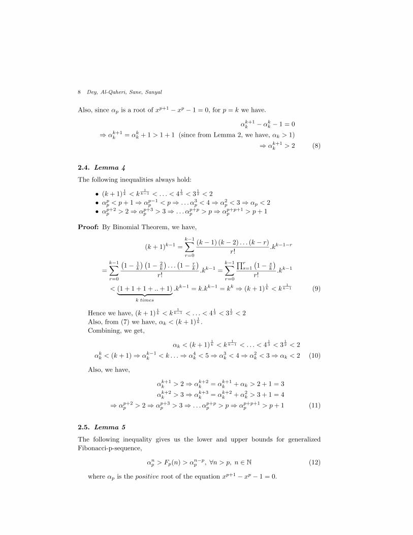
Also, since αp is a root of xp+1 − xp − 1 = 0, for p = k we have.
αk+1k − αkk − 1 = 0
⇒ αk+1k = αkk + 1 > 1 + 1 (since from Lemma 2, we have, αk > 1)
⇒ αk+1k > 2 (8)
2.4. Lemma 4
The following inequalities always hold:
• (k + 1)1k < k
1k−1 < . . . < 4
13 < 3
12 < 2
• αpp < p+ 1⇒ αp−1p < p⇒ . . . α3p < 4⇒ α2
p < 3⇒ αp < 2
• αp+2p > 2⇒ αp+3
p > 3⇒ . . . αp+pp > p⇒ αp+p+1p > p+ 1
Proof: By Binomial Theorem, we have,
(k + 1)k−1 =
k−1∑r=0
(k − 1) (k − 2) . . . (k − r)r!
.kk−1−r
=
k−1∑r=0
(1− 1
k
) (1− 2
k
). . .(1− r
k
)r!
.kk−1 =
k−1∑r=0
∏rs=1
(1− s
k
)r!
.kk−1
< (1 + 1 + 1 + ..+ 1)︸ ︷︷ ︸k times
.kk−1 = k.kk−1 = kk ⇒ (k + 1)1k < k
1k−1 (9)
Hence we have, (k + 1)1k < k
1k−1 < . . . < 4
13 < 3
12 < 2
Also, from (7) we have, αk < (k + 1)1k .
Combining, we get,
αk < (k + 1)1k < k
1k−1 < . . . < 4
13 < 3
12 < 2
αkk < (k + 1)⇒ αk−1k < k . . .⇒ α4k < 5⇒ α3
k < 4⇒ α2k < 3⇒ αk < 2 (10)
Also, we have,
αk+1k > 2⇒ αk+2
k = αk+1k + αk > 2 + 1 = 3
αk+2k > 3⇒ αk+3
k = αk+2k + α2
k > 3 + 1 = 4
⇒ αp+2p > 2⇒ αp+3
p > 3⇒ . . . αp+pp > p⇒ αp+p+1p > p+ 1 (11)
2.5. Lemma 5
The following inequality gives us the lower and upper bounds for generalized
Fibonacci-p-sequence,
αnp > Fp(n) > αn−pp , ∀n > p, n ∈ N (12)
where αp is the positive root of the equation xp+1 − xp − 1 = 0.
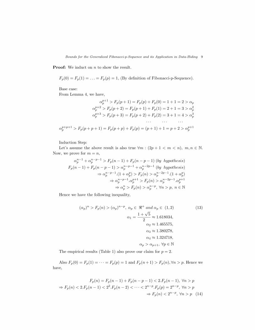
Bounds for the Generalized Fibonacci-p-Sequence and its Application in Data-Hiding 9
Proof: We induct on n to show the result.
Fp(0) = Fp(1) = . . . = Fp(p) = 1, (By definition of Fibonacci-p-Sequence).
Base case:
From Lemma 4, we have,
αp+1p > Fp(p+ 1) = Fp(p) + Fp(0) = 1 + 1 = 2 > αp
αp+2p > Fp(p+ 2) = Fp(p+ 1) + Fp(1) = 2 + 1 = 3 > α2
p
αp+3p > Fp(p+ 3) = Fp(p+ 2) + Fp(2) = 3 + 1 = 4 > α3
p
· · · · · · · · ·αp+p+1p > Fp(p+ p+ 1) = Fp(p+ p) + Fp(p) = (p+ 1) + 1 = p+ 2 > αp+1
p
Induction Step:
Let’s assume the above result is also true ∀m : (2p + 1 < m < n), m, n ∈ N.
Now, we prove for m = n,
αn−1p + αn−p−1p > Fp(n− 1) + Fp(n− p− 1) (by hypothesis)
Fp(n− 1) + Fp(n− p− 1) > αn−p−1p + αn−2p−1p (by hypothesis)
⇒ αn−p−1p .(1 + αpp) > Fp(n) > αn−2p−1p .(1 + αpp)
⇒ αn−p−1p .αp+1p > Fp(n) > αn−2p−1p .αp+1
p
⇒ αnp > Fp(n) > αn−pp , ∀n > p, n ∈ N
Hence we have the following inequality,
(αp)n > Fp(n) > (αp)
n−p, αp ∈ <+ and αp ∈ (1, 2) (13)
α1 =1 +√
5
2≈ 1.618034,
α2 ≈ 1.465575,
α3 ≈ 1.380278,
α4 ≈ 1.324718,
αp > αp+1, ∀p ∈ N
The empirical results (Table 1) also prove our claim for p = 2.
Also Fp(0) = Fp(1) = · · · = Fp(p) = 1 and Fp(n+ 1) > Fp(n),∀n > p. Hence we
have,
Fp(n) = Fp(n− 1) + Fp(n− p− 1) < 2.Fp(n− 1), ∀n > p
⇒ Fp(n) < 2.Fp(n− 1) < 22.Fp(n− 2) < · · · < 2n−p.Fp(p) = 2n−p, ∀n > p
⇒ Fp(n) < 2n−p, ∀n > p (14)

10 Dey, Al-Qaheri, Sane, Sanyal
Combining (13) and (14), we have,
(2)n−p > Fp(n) > (αp)n−p, ∀n > p, and n, p ∈ N (15)
where αp is the positive Root of xp+1 − xp − 1 = 0.
Figure 2 and Table 2 show the convergence of ratio of successive terms for
Fibonacci-p-sequences for different p (For p = 1 we get classical Fibonacci sequence).
It can be noticed that smaller the value of p, quicker the convergence of the ratio is
achieved, as shown. Also value to which the ratio converges monotonically decreases
with increase in the value of p.
3. Application in Data Hiding
Data hiding is a new kind of secret communication technology, where message is
hidden inside an image or any other medium, so that it cannot be observed. One
of the simplest data hiding technique is LSB data hiding technique, which merely
embeds secret message-bits in a subset of the LSB planes of the image. One of the
drawbacks of this technique is: as soon as we go from LSB to MSB for selection
of bit-planes for our message embedding, the distortion in stego-image is likely to
increase exponentially, so it becomes impossible (without noticeable distortion and
with exponentially increasing distance from cover-image and stego-image) to use
higher bit-planes for embedding without any further processing.
This particular problem was addressed by Battisti et al., [Battisti et al. (2006)],
who proposed to use generalized Fibonacci-p-sequence decomposition technique in-
stead of classical binary decomposition and shows by empirical results that this

Bounds for the Generalized Fibonacci-p-Sequence and its Application in Data-Hiding 11
Fig. 2. (a) Convergence of the ratio of successive terms in generalized Fibonacci p-Sequence fordifferent values of p (b) Convergent Subsequences for classical Fibonacci sequence (p=1)
technique outperforms the classical LSB technique when thought in terms of em-
bedding in the higher bit plane as well with less distortion. This technique basically
increases the number of bit-planes (by generating a new larger set of bit-planes
that we call virtual bit-planes) by using Fibonacci-p-sequence decomposition. It
can be further improved using prime and natural number decomposition techniques

12 Dey, Al-Qaheri, Sane, Sanyal
as shown in [Dey et al. (2007a)], [Dey et al. (2007b)], [Dey et al. (2008)]. Also,
[Cooper (1984)] [Dotson et al. (1993)] illustrates Fibonacci sequence can be used in
various applications.
In this paper we give a formal proof of Fibonacci-p-sequence bounds and show
how this can be used to theoretically prove that Fibonacci-p-sequence decomposition
gives better result in hiding data. From (15) it is clear (from the upper bound) that
the same value will require more numbers of bits to be represented than the num-
ber of bits required in classical binary decomposition (since 2n > αn > Fpn), if it’s
expressed using Fibonacci-p-sequence decomposition (where the radix is Fibonacci-
p-sequence numbers instead of powers of 2).
As illustrated in [Dey et al. (2008)], in order to measure the distortion in the
stego-image, we use Mean square error (MSE), Worst case Mean Square Error

Bounds for the Generalized Fibonacci-p-Sequence and its Application in Data-Hiding 13
(WMSE) and Peak Signal to Noise Ratio (PSNR), which are defined by
MSE =
M∑i=1
N∑j=1
(fij − gij)2/MN
PSNR = 10.log10
(L2
MSE
)[Dey et al. (2008)]. If the secret data-bit is embedded in the ith bit-plane of a pixel,
the worst-case error-square-per-pixel will be = WSE = |W (i)(1..0)|2 = (W (i))2
(here W (i) represents the corresponding weight in the number system for the ith bit,
e.g., for classical decomposition W (i) = 2i, for generalized Fibonacci decomposition
W (i) = Fpi), corresponding to the case when the corresponding bit in cover-image
toggles in stego-image, after embedding the secret data-bit. For example, worst-case
error-square-per-pixel for embedding a secret data-bit in the ith bit plane in case
of a pixel in classical binary decomposition is = (2i)2 = 4i, where i ∈ N ∪ {0}.If the original k-bit grayscale cover-image has size w × h, we define, WMSE =
w × h× (W (i))2 = w × h×WSE [Dey et al. (2008)]. Hence,
WMSE after embedding secret message bit only in the lth (virtual) bit-plane of
each pixel in case of classical (traditional) binary (LSB) data hiding technique is
given by, (WMSElthbit−plane
)Classical−Binary−Decomposition = θ(4l).
WMSE after embedding secret message bit in the lth (virtual) bit-plane of each
pixel in case of generalized Fibonacci decomposition is given by,
(WMSElth bit−plane
)Fibonacci−p−Sequence Decomposition = (Fp(l))
2
⇒(α2p
)l−p< (WMSEl)Fibonacci−p−sequence <
(α2p
)l,
αp ∈ <+, α1 =1 +√
5
2,
α2p > α2
p+1,∀p ∈ N, α21 ≈ 2.618,
⇒ (WMSEl)Generalized−Fibonacci−p−sequence < θ(2.618l
).
Hence, we have,
(WMSE)Binary > (WMSE)Fibonacci
⇒ (PSNR)Fibonacci > (PSNR)Binary.
Thus, we have first proved bounds on the generalized Fibonacci sequence and
then by using our bounds, we have given a formal proof for better performance
(in terms of PSNR) for LSB data hiding technique using generalized Fibonacci-p-
sequence decomposition than that using classical binary decomposition. Also, we

14 Dey, Al-Qaheri, Sane, Sanyal
have,
(number of primes ≤ n) = pn = θ(n. log n)
= o(αp)n−p < Fp(n) < 2n−p
([Telang (1999)], [Niven and Zuckerman (1966)], [Tattersall (2005)])
The above implies that if the same number is represented using prime decom-
position (nth prime number as weightage to nth bit), it will give still more numbers
of virtual bit planes [Battisti et al. (2006)].
We have similar results for LSB data hiding using natural number decomposi-
tion technique, and combining the results (from [Battisti et al. (2006)], [Dey et al.
(2007a)], [Dey et al. (2007b)], [Dey et al. (2008)]) we have the following,
(WMSE)Binary > (WMSE)Fibonacci > (WMSE)Prime > (WMSE)Natural
⇒ (PSNR)Natural > (PSNR)Prime > (PSNR)Fibonacci > (PSNR)Binary.
Hence, data hiding using natural number decomposition gives the best perfor-
mance among the above mentioned techniques.
In data hiding, we hide data in different bit-planes of a pixel. In classical LSB
data-hiding technique the pixel is represented as binary value, hence it has less
numbers of bit-planes as we have in case of Fibonacci-p-sequence decomposition,
the later having still less number of bit-planes than in case of prime decomposition
technique. It is shown in [Dey et al. (2007a)], [Dey et al. (2007b)], [Dey et al. (2008)]
by calculation of WMSE and PSNR measures that embedding data even in higher
bit-planes of pixel using these techniques results in less visible distortion of the cover
image, since the distortion as measured by WMSE is proportional to the square of
the weights to the bits in the corresponding decomposition, hence it decreases as the
weights go on decreasing from classical binary to generalized Fibonacci and from
that to prime and natural number decomposition [Dey et al. (2008)].
4. Conclusions
In this paper, we have established the bounds for generalized Fibonacci-sequence
(α)n > Fp(n) > (αp)n−p, ∀n > p, (n, p) ∈ N. Empirical results obtained vindi-
cates our theoretically-proven bounds. Then we used the result (2)n−p > Fp(n) >
(αp)n−p, ∀n > p, (n, p) ∈ N, where αp is the positive Root of xp+1 − xp − 1 = 0, to
prove that data hiding technique using generalized Fibonacci-p-sequence gives more
embeddable bit-planes along with better PSNR than that in case of classical LSB
technique [Dey et al. (2008)], and the same using prime decomposition technique
increases virtual bit-planes and PSNR further [Dey et al. (2007a)].
References
Battisti F., Carli M., Neri A., Egiazarian K. (2006). A Generalized Fibonacci LSB DataHiding Technique. 3rd International Conference on Computers and Devices for Com-munication (CODEC- 06, December 18–20) TEA, Institute of Radio Physics and Elec-tronics, University of Calcutta.

Bounds for the Generalized Fibonacci-p-Sequence and its Application in Data-Hiding 15
Basin S. L. and Hoggatt V. E. Jr. (1963). A Primer on the Fibonacci Sequence, Fib. Quart.1.
Atkins J. and Geist R. (1987). Fibonacci numbers and computer algorithms. College Math.J. 18, 328–337.
Cooper C. (1984). Application of a Generalized Fibonacci Sequence. The College Mathe-matics Journal, Vol. 15, 2, 145–148
Craw I. (2000). Advanced Calculus and Analysis, MA1002, Department of MathematicalSciences, University of Aberdeen, DSN mth200-101982-8, 26–27, V. 1.3.
Dey S., Abraham A. and Sanyal S. (2007a). An LSB Data Hiding Technique Using PrimeNumbers. Third International Symposium on Information Assurance and Security (IAS07, August 29–31), Manchester, United Kingdom, IEEE Computer Society press, USA,ISBN 0-7695-2876-7, 101–106.
Dey S., Abraham A. and Sanyal S. (2007b). An LSB Data Hiding Technique Using NaturalNumbers. IEEE Third International Conference on Intelligent Information Hiding andMultimedia Signal Processing (IIHMSP 07, Nov 26–28), Kaohsiung City, Taiwan, IEEEComputer Society press, USA, ISBN 0-7695-2994-1, 473–476.
Dey S., Abraham A., Bandyopadhyay B. and Sanyal S. (2008). Data Hiding TechniquesUsing Prime and Natural Numbers. Journal of Digital Information Management, Vol.6.
DotsonW., Norwood F. and Taylor C.(1993). Fiber optics and Fibonacci. this MAGAZINE66, 167–174.
Hendel R. J. (1994). Approaches to the formula for the nth Fibonacci number, CollegeMath. J. 25, 139–142.
Hoggatt V. E. Jr. (1972). Fibonacci and Lucas numbers. The Fibonacci Association, SantaClara, California, USA.
Horadam A.(1961). A generalized Fibonacci sequence. American Mathematical Monthly,68, 455–459.
Liu S. H., Chen T. H., Yao H. X., Gao W. (2004). A Variable Depth LSB Data Hid-ing Technique in images. Proceedings of the 3rd International Conference on MachineLearning and Cybernetics, 26-29 August, Shanghai.
Niven I. and Zuckerman H. S. (1966). An Introduction to the Theory of Numbers. Wiley,2nd ed., New York.
Picione D. D. L., Battisti F., Carli M., Astola J. and Egiazarian K.(2006). A FibonacciLSB data hiding technique. Proc. European signal processing conference.
Sun Z. H. and Sun Z. W. (1992). Fibonacci numbers and Fermat’s last theorem. ActaArith. 60, 371–388.
Tattersall J. J. (2005). Elementary number theory in nine chapters, 2nd ed., CambridgeUniversity Press, ISBN 9780521850148, 28–31.
Telang S. G. (1999). Number Theory. Tata McGraw-Hill, ISBN 0-07-462480-6, FirstReprint, 617–631.
Wang R. Z., Lin C. F. and Lin I. C. (2001). Image Hiding by LSB substitution and geneticalgorithm. Pattern Recognition, Vol. 34, 3, 671–683.
Top Related
Copyright © 2022 FDOKUMEN

