Download - A NIKA view of two star-forming infrared dark clouds - arXiv

Astronomy & Astrophysics manuscript no. main c©ESO 2018February 19, 2018

A NIKA view of two star-forming infrared dark clouds:Dust emissivity variations and mass concentration

A. J. Rigby1, N. Peretto1, R. Adam2, 3, P. Ade1, P. André4, H. Aussel4, A. Beelen5, A. Benoît6, A. Bracco4,A. Bideaud6, O. Bourrion2, M. Calvo6, A. Catalano2, C. J. R. Clark1, B. Comis2, M. De Petris7, F.-X. Désert8,

S. Doyle1, E. F. C. Driessen9, J. Goupy6, C. Kramer10, G. Lagache11, S. Leclercq9, J.-F. Lestrade12,J. F. Macías-Pérez2, P. Mauskopf1, 13, F. Mayet2, A. Monfardini6, E. Pascale1, L. Perotto2, G. Pisano1, N. Ponthieu8,

V. Revéret4, A. Ritacco10, C. Romero9, H. Roussel14, F. Ruppin2, K. Schuster9, A. Sievers10, S. Triqueneaux6,C. Tucker1, and R. Zylka9

1 School of Physics & Astronomy, Cardiff University, Queen’s Buildings, The Parade, Cardiff, CF24 3AA, UKe-mail: [email protected]

2 Laboratoire de Physique Subatomique et de Cosmologie, Université Grenoble Alpes, CNRS/IN2P3, 53, avenue des Martyrs,Grenoble, France

3 Laboratoire Lagrange, Université Côte d’Azur, Observatoire de la Côte d’Azur, CNRS, Blvd de l’Observatoire, CS 34229, 06304Nice cedex 4, France

4 Laboratoire AIM, CEA/IRFU, CNRS/INSU, Université Paris Diderot, CEA-Saclay, 91191 Gif-Sur-Yvette, France5 Institut d’Astrophysique Spatiale (IAS), CNRS and Université Paris Sud, Orsay, France6 Institut Néel, CNRS and Université Grenoble Alpes, France7 Dipartimento di Fisica, Sapienza Università di Roma, Piazzale Aldo Moro 5, I-00185 Roma, Italy8 Institut de Planétologie et d’Astrophysique de Grenoble, Univ. Grenoble Alpes, CNRS, IPAG, 38000 Grenoble, France9 Institut de RadioAstronomie Millimétrique (IRAM), Grenoble, France

10 Institut de RadioAstronomie Millimétrique (IRAM), Granada, Spain11 Aix Marseille Université, CNRS, LAM (Laboratoire d’Astrophysique de Marseille) UMR 7326, 13388, Marseille, France12 LERMA, CNRS, Observatoire de Paris, 61 avenue de l’Observatoire, Paris, France13 School of Earth and Space Exploration and Department of Physics, Arizona State University, Tempe, AZ 8528714 Institut d’Astrophysique de Paris, CNRS (UMR7095), 98 bis boulevard Arago, F-75014, Paris, France

Received ; accepted

ABSTRACT

Context. The thermal emission of dust grains is a powerful tool for probing cold, dense regions of molecular gas in the interstellarmedium, and so constraining dust properties is key to obtaining accurate measurements of dust mass and temperature.Aims. By placing constraints on the dust emissivity spectral index, β, towards two star-forming infrared dark clouds – SDC18.888-0.476 and SDC24.489-0.689 – we aim to evaluate the role of mass concentration in the associated star-formation activity.Methods. We exploited the simultaneous 1.2 mm and 2.0 mm imaging capability of the NIKA camera on the IRAM 30 m telescopeto construct maps of β for both clouds, and by incorporating Herschel observations, we created H2 column density maps with 13′′angular resolution.Results. While we find no significant systematic radial variations around the most massive clumps in either cloud on & 0.1 pcscales, their mean β values are significantly different, with β = 2.07 ± 0.09 (random) ±0.25 (systematic) for SDC18.888-0.476 andβ = 1.71 ± 0.09 (random) ±0.25 (systematic) for SDC24.489-0.689. These differences could be a consequence of the very differentenvironments in which both clouds lie, and we suggest that the proximity of SDC18.888-0.476 to the W39 H ii region may raise βon scales of ∼ 1 pc. We also find that the mass in SDC24.489-0.689 is more centrally concentrated and circularly symmetric thanin SDC18.888-0.476, and is consistent with a scenario in which spherical globally-collapsing clouds concentrate a higher fraction oftheir mass into a single core than elongated clouds that will more easily fragment, distributing their mass into many cores.Conclusions. We demonstrate that β variations towards interstellar clouds can be robustly constrained with high signal-to-noiseratio (S/N) NIKA observations, providing more accurate estimates of their masses. The methods presented here will be applied tothe Galactic Star Formation with NIKA2 (GASTON) guaranteed time large programme, extending our analysis to a statisticallysignificant sample of star-forming clouds.

Key words. stars: formation – submillimetre:ISM – ISM: clouds – ISM: dust – ISM: structure

1. Introduction

Despite making up only ∼1% of the mass of the interstellarmedium (ISM), dust grains are central to studies of molecu-lar clouds and star formation. Dust grains are a robust tracerof molecular gas density over many orders of magnitude while

playing a major role in facilitating the formation of moleculesand being an important element of the cooling system of theISM. Observations of dust extinction or emission – typically ob-servable from the infrared to millimetre wavelengths – allow thedetermination of the masses and temperatures of ISM structures,

Article number, page 1 of 18

arX

iv:1

801.

0980

1v2

[as

tro-

ph.G

A]

16

Feb

2018

A&A proofs: manuscript no. main

providing important constraints on the energy balance of objectsat various stages of the star-forming process.

Such mass and temperature determinations depend on theproperties of the dust grains, whose composition, size distribu-tion and morphology are usually embodied in the dust emissiv-ity, κν. In the far-infrared to millimetre regime, where most of theenergy from interstellar dust grains is radiated, the emissivity isoften described as a single power law:

κν = κ0

(λ

λ0

)−β= κ0

(ν

ν0

)β, (1)

where κ0 is the dust opacity at a reference wavelength λ0 (orfrequency ν0), and β the dust emissivity spectral index. Althoughit is common practice to assume a uniform dust emissivity law,there is growing evidence that it depends on the environment,through ice coating processes and subsequent dust coagulation,changing both its shape – β – and normalisation – κ0/λ0 (e.g.Ossenkopf & Henning 1994; Cambrésy et al. 2001; Ormel et al.2011; Ysard et al. 2013). For example, the presence of large dustparticles towards pre-stellar cores was directly highlighted bythe observation of ‘coreshine’, that is scattered light at 3–5 µm(Steinacker et al. 2010; Pagani et al. 2010), which can only beaccounted for by the presence of a population of micron-sizedgrains.

The characterisation of β, and its anti-correlation with dusttemperature, has been the subject of a large number of studies(e.g. Dupac et al. 2003; Désert et al. 2008; Shetty et al. 2009;Smith et al. 2012; Sadavoy et al. 2013; Juvela et al. 2015; Chenet al. 2016; Sadavoy et al. 2016). This is most often achievedby fitting the spectral energy distribution (SED) around its emis-sion peak with a modified black-body function whose temper-ature, dust mass surface density, and emissivity spectral in-dex are left as free parameters. However, moderate noise lev-els lead to model degeneracy between temperature and spec-tral index, potentially explaining part of the often-observed anti-correlation between these two parameters (Shetty et al. 2009).Chen et al. (2016) find that the Td−β anti-correlation is signifi-cant in Perseus even after accounting for the noise-related degen-eracy, with 1.0 . β . 2.7. Grain growth in cold dense regionspushes β to low values, though the formation of ice mantles cansuppress grain growth to increase β, leading Chen et al. (2016)to propose the sublimation of ice mantles in warm regions asan explanation for the Td−β anti-correlation. β generally reacheslower values at the locations of protostellar sources. Dupac et al.(2003) and Yang & Phillips (2007) found very similar ranges ofβ in nearby star-forming clouds and across a sample of luminousinfrared galaxies, respectively. The Planck Collaboration XXV(2011) also reported a Td−β anti-correlation that could not beexplained by noise alone in Taurus, finding an average value ofβ ≈ 1.8 ± 0.2.

Another way of constraining β is by observing dust emissionat two, or more, wavelengths in the millimetre regime. As onemoves closer to the Rayleigh-Jeans tail of the SED, the intensityratio of these wavelengths becomes less dependent on tempera-ture, greatly reducing the effect of the Td−β degeneracy. Sadavoyet al. (2013) used SCUBA-2 maps of the ratio of 450 µm and850 µm imaging towards several low-mass nearby star-formingregions in the Gould Belt Survey. The authors note that, whilethe two wavelengths alone can not be used to simultaneouslyconstrain Td and β, relative variations in the latter can be studiedif the dust temperature is roughly constant. One issue with theseresults is that despite the data being at longer wavelengths than

most Herschel bands, they are not still far enough from the peakof the SED to totally lift the Td−β degeneracy, and a differencein dust temperature of 6 K results in a shift in β values by ≈ 0.86.

More recently, Bracco et al. (2017) used the New IRAMKIDs Array (NIKA) prototype millimetre camera on the Institutde Radioastronomie Millimétrique (IRAM) 30-m telescope toconstrain β in the Taurus B213 filament. By using an Abel trans-form technique in conjunction with the intensity ratio methodusing 1.2 mm and 2.0 mm continuum images, they were ableto simultaneously determine radial temperature and β profiles intwo low-mass protostellar cores and one pre-stellar core, find-ing β profiles with low central values of β ≈ 1.0 and 1.5 in theprotostellar cores, from which β increases radially, while the pre-stellar core is consistent with a single β value of 2.4. By observ-ing dust emission simultaneously at 1.2 mm and 2.0 mm, NIKAobservations take us closer to the Rayleigh-Jeans regime, allow-ing a more robust determination of β.

Infrared dark clouds (IRDCs) are cold and dense molecu-lar clouds identified in absorption against the mid-infrared back-ground of the Galaxy (e.g. Simon et al. 2006; Peretto & Fuller2009). In the past decade or so, IRDCs have been privileged tar-gets for studying the earliest stages of star formation. One keyreason for this is that the low number of embedded young stel-lar objects within IRDCs ensures that the initial conditions forstar formation are still imprinted in the IRDC gas properties. Byusing dendrograms on column density maps (see Rosolowskyet al. 2008 for an introduction to dendrograms), Kauffmann et al.(2010a,b) showed that the mass-size relationship of the identifiedsubstructures within a cloud can be linked to the ability of thecloud to form high-mass stars. According to this relation, onlya small fraction of known IRDCs have the required conditionsto form high-mass stars. These clouds are, therefore, excellenttargets to study the early stages of high-mass star formation.

Peretto & Fuller (2009) identified a sample of ∼11,000IRDCs in the Galactic plane in the range 10 < |`| < 65 and|b| < 1 by using 8 µm Spitzer GLIMPSE (Benjamin et al. 2003)and 24 µm MIPSGAL (Carey et al. 2009) data. In this study, wefocus on two IRDCs from the Peretto & Fuller (2009) catalogue,SDC18.888-0.476 and SDC24.489-0.689 (hereafter SDC18 andSDC24, respectively), located at ` = 18.888, b = −0.476 and` = 24.489, b = −0.689. The two IRDCs also form part ofthe dense gas survey from Peretto et al. (in prep.) and were tar-geted in this study because of their differences in morphology,masses, sizes, and mid-IR environment. Systemic velocities inN2H+ (1−0) were measured by Peretto et al. (in prep) to be+66.3 km s−1 and +48.1 km s−1, yielding kinematic distances of4.38 ± 0.27 kpc and 3.28 ± 0.34 kpc, respectively, adopting theReid et al. (2009) Galactic rotation model. SDC18 lies on theedge of the W39 H ii region, a region of widespread active high-mass star formation (HMSF; Kerton et al. 2013), and harboursan Extended Green Object at its centre (Cyganowski et al. 2008).By contrast, SDC24 is relatively secluded, with no H ii regionidentified in the area. Only an outflow, identified by H2 knots,has been associated with a young stellar object (YSO) locatedtowards the centre of the cloud (Ioannidis & Froebrich 2012).

Here, we use NIKA data to constrain, for the first time, βvariations within two infrared dark clouds (IRDCs) and to usethese results to characterise the mass concentration within theIRDCs as a function of their global properties. This paper isdivided into the following Sections. In Section 2 we describethe observations, data reduction and calibration. We describe ourmethodology for the β determination in Section 3 and our massdetermination is presented in Section 4. A discussion of the im-


A. J. Rigby et al.: A NIKA view of two star-forming infrared dark clouds

plications of the results follows in Section 5, and we summariseour results to conclude in Section 6.

2. Observations

2.1. NIKA data

We used NIKA (Monfardini et al. 2010, 2011; Catalano et al.2014) on the IRAM 30 m telescope to map SDC18 and SDC24simultaneously in the 1.2 mm and 2.0 mm continuum wave-bands. The observations were made on November 16th 2014 aspart of the NIKA Open Pool 2 campaign and reduced follow-ing the procedures described in Catalano et al. (2014) and Adamet al. (2014). Mean zenith opacities at 225 GHz for SDC18 andSDC24 were τ225 = 0.23 and 0.20, and the mean elevations were45 and 35, respectively.

The NIKA maps were calibrated using observations ofUranus at reference frequencies of 260 GHz and 150 GHz forthe 1.2 mm and 2.0 mm bands, respectively. Since the IRDCshave SEDs which differ to that of Uranus, a colour correc-tion must be applied that accounts for the response of the twoNIKA bandpasses as a function of frequency, effectively convert-ing the fluxes to monochromatic values at the nominal frequen-cies. The model of Moreno (2010)1 was adopted for the SED ofUranus. The colour correction assumes a source SED of the formf (ν/ν0) = (ν/ν0)α, and we adopted a value of α = 3.8 for sourcesdescribed by a modified black-body model in the Rayleigh-Jeanslimit, with dust emissivity spectral index β = 1.8, which isthe average value in the Milky Way disk (Planck CollaborationXXV 2011). The colour correction factors were determined tobe Ccol = 0.971 and 0.917 for the 1.2 mm and 2.0 mm bands,where S corr = S obs ×Ccol based on this assumed spectral shape.

Uranus observations were also used to determine the pro-file of the primary telescope beam. The main beam of the tele-scope is well fitted by a Gaussian distribution with a full-widthhalf-maximum (FWHM) of 12.0′′ and 18.2′′ for the 1.2 mm and2.0 mm wavebands, respectively (Ruppin et al. 2017), thoughwe note that for extended emission, there are significant non-Gaussian sidelobes at large radii which should be accounted for.The Uranus observations were also used to determine the effec-tive solid angle ΩA of the 1.2 mm and 2.0 mm beams, whichwere measured to be 4.51 × 10−9 sr and 10.99 × 10−9 sr, respec-tively, allowing the raw maps to be converted from their intrinsicunits of Jy beam−1 to MJy sr−1. We summarise the basic prop-erties of the NIKA images, and those from the other observa-tions used in this study in Table 1. The NIKA images are pre-sented in Fig. 1 alongside 8 µm images from the Spitzer surveyGLIMPSE in which the IRDC components were originally iden-tified by Peretto & Fuller (2009).

The rms noise levels in the NIKA images vary according toposition as a consequence of the scanning pattern and the re-duced integration time per pixel at the image edges. However,noise levels are relatively constant within ∼ 1.8′ of the centrein SDC18, or within ∼ 1.2′ of the centre of SDC24, which isapproximately where the main emission features lie. The centralrms noise values in both pairs of 1.2 mm and 2.0 mm images forSDC18, once slightly smoothed to effective angular resolutionsof 13′′ and 20′′ (and before application of the colour corrections)are 7.1 mJy beam−1 and 2.2 mJy beam−1, respectively, while forSDC24 the central rms noise values are 4.8 mJy beam−1 and 0.9mJy beam−1, respectively. Details of the rms noise levels andmean background levels in units of MJy sr−1 are presented inTable 2.1 ftp://ftp.sciops.esa.int/pub/hsc-calibration/PlanetaryModels/ESA2/

Extended emission on scales larger than the ∼ 2′ field ofview is removed during the atmospheric decorrelation of the rawNIKA timelines, in which it is impossible to distinguish betweenastrophysical and atmospheric signal. Consequently, the 1.2 mmand 2.0 mm NIKA images of SDC18, which lies in a region ofbright extended emission (as seen in the Spitzer images of Fig.1) contain a region of negative emission towards the centre. Thespatial filtering has the effect of reducing the flux in every pixel,and while the effect is small in regions where the emission iscompact, such as towards the emission peaks, it can be large indiffuse regions. We discuss the impact of this filtering upon ourresults in the relevant Sections of this paper.

2.2. Herschel data

Data from the Herschel infrared Galactic Plane Survey (Hi-GAL; Molinari et al. 2010, 2016), consisting of PACS (Poglitschet al. 2010) imaging at 70 and 160 µm, and SPIRE (Griffin et al.2010) imaging at 250, 350, and 500 µm were also used. We usedthe DR1 versions of the photometric maps, described in Molinariet al. (2016), which have been reduced using the ROMAGALdata reduction pipeline, described in Traficante et al. (2011). Aspart of DR1, the reduced maps have been calibrated to a com-mon zero level with offsets determined by comparison to all-skymaps from Planck and IRIS, following the process outlined inBernard et al. (2010).

The Herschel images are calibrated assuming a flat sourcespectrum, that is Iν ∝ ν−1. We adopted the colour correc-tions determined by Sadavoy et al. (2013), who found Ccol =1.01, 1.02, 1.01 and 1.03 for the 160, 250, 350 and 500 µmbands, respectively, for extended sources with dust temperaturesof Td ≈ 10 − 15 K and dust emissivity spectral indices ofβ ≈ 1.5−2.5. It is not necessary to apply any colour correction tothe 70 µm, given its minor role in this study. We adopt absolutecalibration uncertainties at the level of 5% for PACS and 4% forSPIRE imaging (Molinari et al. 2016) throughout this study.

2.3. ATLASGAL data

In addition to the NIKA and Hi-GAL continuum imaging, wemade use of the ATLASGAL survey (Schuller et al. 2009) whoseobservations were made using the LABOCA camera (Siringoet al. 2009). These data have an angular resolution of 19.2′′,and are calibrated on planet observations with a spectrum ofIν ∝ ν2 and a reference frequency of 345 GHz. We applied acolour correction factor of 0.988 to the data, following Csengeriet al. (2016), in order to match the SED assumption made tocalculate the NIKA colour correction in Sect. 2.1 – a modifiedblack-body with β = 1.8. All colour corrections applied to thevarious data in this study are summarised in Table 1.

2.4. MAGPIS data

Data from the Multi-Array Galactic Plane Imaging Survey(MAGPIS; Helfand et al. 2006) were also used in this work.The 20 cm continuum MAGPIS data were taken from the VeryLarge Array (VLA) in pseudocontinuum mode in B, C and D-configurations, providing a sensitivity of 1–2 mJy with a 6′′-resolution synthesised beam. The Image Cutout service2 wasused to extract 10′ × 10′ 20cm continuum images covering theSDC18 and SDC24 NIKA fields, which have rms noise valuesof 0.2 mJy beam−1 and 0.3 mJy beam−1, respectively.

2 https://third.ucllnl.org/cgi-bin/gpscutout



Fig. 1. Top row: images of SDC18, with Spitzer 8 µm images in yellow, followed by the 1.2 mm and 2.0 mm NIKA images, slightly smoothed to13 and 20 arcseconds resolution, respectively. Bottom row: as above for SDC24. The contours on the 8 µm images show the where S/N=3 fromthe 13-arcsecond resolution 1.2 mm images.

Table 1. Details of the wavebands of the various single-dish observations used in this study. For the LABOCA and NIKA images, we detail theeffective beam solid angles used to convert the images into units of MJy sr−1, though we note that the Hi-GAL images are supplied in units ofMJy sr−1. The nominal wavelengths or frequencies recovered after colour correction are denoted in each case are denoted by an asterisk, andbandwidths are quoted in corresponding units.

Facility Instrument λ0 ν0 FWHM ΩA Bandwidth Ccol(µm) (GHz) (arcsec) (10−9 sr) (µm, GHz)

Herschel PACS 70* 4280 6.0a – 60–85c 1.00PACS 160* 1870 12.0a – 130–210c 1.01SPIRE 250* 1200 18.0 – 211–290c 1.02SPIRE 350* 857 24.0 – 297–405c 1.01SPIRE 500* 600 35.0 – 409-611c 1.03

APEX LABOCA 869 345* 19.2 12.17b 313–372c 0.988

IRAM NIKA 1153 260* 12.0 4.51 196–273d 0.97130-m NIKA 1999 150* 18.2 10.99 127–171d 0.917

Notes.(a) We note that the 70 µm and 160 µm Hi-GAL images do not achieve the nominal beam size, but instead have PSFs that are elongated in the scandirection, and are measured to be 5.8′′ × 12.1′′ and 11.4′′ × 13.4′′, respectively. See Molinari et al. (2016) for more details.(b) We adopt the LABOCA total beam area for extended sources. See http://www.apex-telescope.org/bolometer/laboca/calibration/.(c) The PACS, SPIRE and LABOCA waveband edges are defined as half of the average in-band transmission (Siringo et al. 2009; Poglitsch et al.2010; Swinyard et al. 2010).(d) The NIKA waveband edges contain ninety percent of the total transmission (Adam et al. 2014).

3. Constructing β maps using NIKA data

NIKA observations provide a powerful complement to Her-schel data by providing greater angular resolution at wavelengthslonger than 500 µm in the spectral energy distributions of ther-mal dust emission. These can be used to better constrain thespectral index of the dust emissivity, thus providing tighter con-straints on the dust masses, as well as improving the identifica-tion of cold compact sources and underlying dust structure in

each IRDC. In this Section we describe the steps necessary toconstruct maps of β using NIKA data and discuss the nature ofthe related uncertainties.

3.1. Clump properties

Both SDC18 and SDC24 contain one dominant compact clumpwhich contains the majority of the dust emission, centred on ` =18.887, b = -0.474and ` = 24.488, b = -0.691, respectively.


http://www.apex-telescope.org/bolometer/laboca/calibration/


Table 2. Statistics of NIKA images under various levels of smoothing.Individual images are denoted by the approximate central wavelengthλ in the corresponding waveband, with an effective resolution elementof FWHM θ after smoothing. Smoothing using kernels denoted ‘G’ areGaussian, while those denoted ‘P’ used the PSF-matching kernel de-scribed in Sect 3.2, and where no kernel is listed, measurements of theraw (unsmoothed) data are presented. We also list the mean integrationtime, tobs per 2′′ pixel in the central 1.8′ in SDC18 and 1.2′ in SDC24used to calculate the effective rms noise level σ and mean backgroundlevel µ.

Source λ θ Kernel tobs µ ± σ(mm) (′′) (s/pix) (MJy sr−1)

SDC18 1.2 12.0 – 20.6 −0.10 ± 2.351.2 13.0 G 20.6 0.14 ± 1.571.2 20.0 P 20.5 0.17 ± 1.151.2 20.0 G 20.5 0.17 ± 1.162.0 18.2 – 15.9 0.01 ± 0.292.0 20.0 G 15.9 0.02 ± 0.20

SDC24 1.2 12.0 – 17.9 −0.03 ± 2.131.2 13.0 G 17.8 0.15 ± 1.011.2 20.0 P 17.8 0.12 ± 0.621.2 20.0 G 17.8 0.12 ± 0.602.0 18.2 – 13.6 0.00 ± 0.282.0 20.0 G 13.6 0.00 ± 0.09

To acquire an initial estimate of the properties of these clumps,their spectral energy distributions (SEDs) were measured, andfitted to a modified black body model, which has a flux densityIν at a frequency ν given by:

Iν = NH2µH2 mHκ0

(ν

ν0

)βBν(Td), (2)

where NH2 is the H2 column density, µH2 is the mean molecu-lar weight per hydrogen molecule which has a value of 2.8 formolecular gas with a relative Helium abundance of 25%, mH isthe mass of a hydrogen atom, κ0 is the specific dust opacity at thereference frequency ν0, β is the dust emissivity spectral index,and Bν(Td) is the Planck function evaluated at the dust tempera-ture Td. It is important to bear in mind that these quantities arenecessarily line-of-sight averages. We stress that the SED-fittingprocedure provides an initial estimate of the clump properties,and in particular the dust temperature which will be required toproduce β maps in Section 3.4. It is, therefore, subject to the Td-β degeneracy though this should be expected to have the samesystematic effect for both sources.

To supplement the 1.2 mm and 2.0 mm NIKA images, Hi-GAL 160 µm and 250 µm images as well as ATLASGAL 870µm images, which all have comparable or better angular resolu-tion than the NIKA imaging, were used to constrain the SEDs.Before constructing SEDs we resampled the Hi-GAL and AT-LASGAL images on to the same 2′′-pixel grid as the NIKA data.As a consequence all images were largely oversampled, but thiswas necessary to check for astrometric consistency between thedifferent telescopes. A systematic shift of +4′′ in declination wasfound in the Hi-GAL data compared to the NIKA and ATLAS-GAL data, which was estimated by comparing the emission cen-troid of the three main emission peaks in the Herschel 250 µmand NIKA 1.2 mm images, and the Hi-GAL images were ac-cordingly shifted by ∆δ = −4′′ to account for this discrepancy.

As space-based observations, the Hi-GAL images recover in-tensity on all angular scales, in contrast to the ground-based AT-

0 1 2 3 4 5 6Wavenumber [arcmin 1]

0.0

0.2

0.4

0.6

0.8

1.0

Tran

smiss

ion

Fiel

d of

vie

w

1.2

mm

bea

m

2.0

mm

bea

m

Fig. 2. Transfer function for NIKA data reduced in this study. The verti-cal lines identify spatial frequencies associated with the 1.9′ NIKA 2.0mm field of view (for clarity we do not also show the 1.8′ field of viewat 1.2 mm), as well as the corresponding FWHM beam sizes in bothwavebands. The dashed part of the transfer functions have been extrap-olated to a zero-level of transmission at a wavenumber of 0 arcmin−1.

LASGAL and NIKA imaging which necessarily lose flux fromlarge-scale emission as a result of the filtering of atmosphericfluctations in the data reduction processes. Comparison of thefluxes from the ground- and space-based images should ideallycontain the same sensitivity to all scales of emission, and so weconstructed a transfer function for NIKA to apply equivalent spa-tial filtering to the Herschel observations. To achieve this, a se-ries of synthetic images with defined angular power spectra weregenerated and processed through the same reduction pipeline aswas used for the raw observations of SDC18 and SDC24. Thepower spectra of the output maps, computed with POKER (Pon-thieu et al. 2011), were then compared to those of the input mapsin order to construct an average transfer function for both NIKAwavelengths, which we display in Fig. 2. After application ofthe appropriate transfer function, the Herschel images can be re-garded as being equivalently spatially filtered. We applied the1.2 mm and 2.0 mm NIKA transfer functions to the 160 µm and250 µm Herschel images, respectively, as these wavebands havewell-matched angular resolutions. We applied no further filteringto the ATLASGAL data, noting that LABOCA will have recov-ered more extended emission since it has a larger field of viewthan NIKA (with a diameter of 11′ compared to 2′, respectively),and therefore will contain an additional flux contribution fromextended emission.

The Python package photutils was used to carry out aper-ture photometry on each clump, using an aperture with a 25′′ ra-dius, equal to ∼ 3 times the standard deviation of the LABOCAbeam, which has the lowest angular resolution. An annular skyaperture was used with inner and outer radii equal to 1.5 and2.0 times that of the source aperture, respectively. The rms noiselevel was determined in each image after applying 50 iterationsof sigma-clipping with a 2.5 sigma cut-off. At each wavelength,the rms uncertainties only contribute a relatively small uncer-tainty to the integrated fluxes, whose errors are dominated bythe calibration uncertainties. The calibration uncertainties weretaken to be 5% for the unfiltered Herschel PACS band at 160 µm(Molinari et al. 2016), 4% for the unfiltered Herschel SPIRE 250µm band (Molinari et al. 2016), 15% for the 870 µm ATLAS-



100 1000Wavelength [ m]

10 2

10 1

100

101

102

103

Flux

den

sity

[Jy]

Rap = 25 arcsecSDC18N(H2) = 1.59 ± 0.72 × 1023 cm 2

= 2.39 ± 0.18Td = 14.32 ± 1.36 K

2dof = 0.69

SDC24N(H2) = 3.83 ± 1.72 × 1022 cm 2

= 1.89 ± 0.18Td = 14.15 ± 1.32 K

2dof = 0.10

Fig. 3. SED fits for the main clumps in SDC18 (red) and SDC24 (blue),along with the best fit parameters. The aperture photometry measure-ments are shown as filled circles for SDC18 and filled triangles forSDC24. We show the measurements at 70 µm, 350 µm and 500 µmthat were not used in the fitting procedure as empty symbols.

GAL image (Schuller et al. 2009), and 11% and 9% for the 1.2mm and 2.0 mm NIKA bands, respectively (Ruppin et al. 2017).We applied no aperture corrections to the aperture photometrymeasurements on the basis that the sources are extended.

After our application of the NIKA transfer function to theHi-GAL data, we must increase the flux uncertainties measuredin the apertures accordingly. The absolute calibration uncertain-ties for the NIKA images, determined by Catalano et al. (2014),contains a 5% contribution from the spatial filtering in the caseof point sources. Since we are looking at dense cores that aremarginally resolved in the NIKA data, the spatial filtering mustcontribute a minimum of 5% uncertainty, but should be of a sim-ilar order of magnitude. By comparing the mean aperture flux inthe filtered and unfiltered 160 µm and 250 µm Herschel bands,weighted by the 1.2 mm intensity per pixel, we conservativelyestimate that the NIKA transfer function contributes an addi-tional fractional uncertainty of 12% to the filtered Herschel im-ages.

The SED fitting was performed using the Python SciPyroutine curve_fit, which performs a χ2 minimisation via theLevenberg–Marquardt algorithm. Figure 3 shows the measuredSEDs for SDC18 and SDC24 along with the modified blackbody fits along with the best fit parameters. The dust tempera-tures are consistent with each other, with a value of 14.32± 1.36K in SDC18 and 14.15 ± 1.32 in SDC24. The average columndensities per 2′′ pixel within the 25′′ apertures are 1.6±0.7×1023

cm−2 and 3.8 ± 1.7 × 1022 cm−2 for SDC18 and SDC24, respec-tively, which yield masses of 3200±1500 M and 430±210 M.At distances of 4380 pc and 3280 pc, a 25′′ aperture correspondsto ∼0.5 pc and ∼0.4 pc, respectively. In Fig. 3 we also include theaperture photometry measurements in the 70 µm band, though itshould be noted that these points were not used in the SED-fittingas 70 µm emission often contains non-equilibrium dust heatingfrom embedded young stellar objects (Dunham et al. 2008). Wewere unable to spatially filter the 350 µm and 500 µm Herschelimages in a way that is consistent with the NIKA data pointssince their beamsizes are considerably larger (indeed, the close

match of the resolutions of the 160 µm and 250 µm Herschelimages with the 1.2 and 2.0 mm NIKA images is fortuitous).We include the photometric measurements from these imagesin Fig. 3 after applying the 2.0 mm NIKA transfer function forclarity, but note that the filtering is necessarily too harsh due toits determination from a smaller beamsize, which results in un-derestimated fluxes. We note that the χ2 per degree of freedomvalue for SDC24 is rather low (see Fig. 3), and we can only re-cover a value of unity by artificially decreasing the uncertaintiesresulting from the absolute calibration to an unrealistic level. Weinterpret this as an indication that there may be some level of cor-relation between uncertainties that we have not accounted for inthis approach, and the two NIKA wavebands must be the primecandidate. However, investigating potential correlations betweenthe NIKA calibrations is beyond the scope of this paper.

3.2. Constructing a PSF-matching convolution kernel

The 1.2 mm and 2.0 mm NIKA wavebands have different an-gular resolutions and so a common resolution must be achievedbefore comparison of the intensities of pixels covering the sameareas of sky can be used to derive physical quantities. A standardmethod of achieving this is to use Gaussian smoothing kernels,where the quadrature sum of the FWHMs of the beam and thesmoothing kernel is equal to that of the desired common resolu-tion. In principle, this method will work well for telescope beamsthat follow a Gaussian profile, but the two NIKA beams show asignificant departure from a Gaussian profile in the sidelobes.The NIKA sidelobes can contain as much as 43% of the power(Catalano et al. 2014) in the point spread function (PSF), andneglect of this matter may introduce artificial features in subse-quent analyses.

To effectively match the PSFs in maps made in the two NIKAwavebands, we created a PSF-matching kernel that, when ap-plied to the 1.2 mm imaging, will result in an image with thesame effective PSF as the 2.0 mm image. The psf.matching sub-package of the photutils (Bradley et al. 2016) Python packagewas used to generate a convolution kernel using the ratio of thefast Fourier transforms (FFTs) of the 1.2 mm and 2.0 mm PSFs(e.g. Gordon et al. 2008; Aniano et al. 2011; Pattle et al. 2015).The NIKA PSFs were constructed by taking the mean of threebeam maps made from observations of Uranus on the nights ofthe 19th and 20th of February 2014 during the preceding observ-ing campaign. Prior to taking the mean value of each pixel in thebeam maps, the maps were normalised to the peak intensity toensure a consistent scaling and then circularly averaged follow-ing the method described in Section 4.4 of Aniano et al. (2011).The PSFs have been spatially filtered to reduce the impact ofhigh frequency noise arising from finite numerical precision. Weused a Top Hat window function to exclude spatial frequencieswith an intensity of less than 0.5% of the maximum value ofthe 1.2 mm PSF’s FFT. In this way, spatial frequencies higherthan 40% of the highest frequency (corresponding to a 2 pixel-wavelength oscillation) were removed.

Radial profiles of the circularly-averaged NIKA beams arepresented in Fig. 4, along with profiles of 1.2 mm beam afterconvolution with the PSF-matching kernel and a Gaussian ker-nel for comparison. The middle and lower panels show the dif-ference and ratio between the 1.2 mm profiles convolved usingthe two methods and the 2.0 mm profile. The middle panel showsthat the PSF-matching kernel is able to map the 1.2 mm PSF onto the 2.0 mm PSF extremely well, and has a better than 1%agreement, assuming circular symmetry, up to a radius of 4′. Bycomparison, resolution-matching using a purely Gaussian kernel



10 5

10 4

10 3

10 2

10 1

100

Rela

tive

beam

resp

onse

1.2 mm2.0 mm1.2 mm * kG1.2 mm * kP

0.060.040.020.00

Diffe

renc

e

0 50 100 150 200 250Radius [arcsec]

0.00.51.01.52.0

Ratio

Fig. 4. Profiles of the 2.0 mm NIKA beam (red line), alongside the1.2 mm NIKA beam before (blue line) and after convolution with theGaussian (grey line) and PSF-matching kernels (black dashed line). Thebottom two panels show the differences between, and the ratios of, thetwo 1.2 mm beam profiles smoothed to the 2.0 mm resolution using theGaussian and PSF-matching kernels and the 2.0 mm profile. Bucklingof the panels of the primary mirror show up as features at ∼ 2′ and 3.5′in the average 1.2 mm and 2.0 mm beam profiles, respectively.

results in a significant departure at radii up to ∼ 20′′ that couldbe particularly problematic for compact sources. Indeed, in thelower panel, showing the ratio between the convolved 1.2 mmprofiles and the 2.0 mm profile, it can be seen that the Gaus-sian convolution method causes an artificial change in the ratioof 50% at around 20′′, though while there are much larger devia-tions at larger radii, the power in the beam beyond 60′′ is so lowas to have no effect on these images.

Finally, NIKA maps of SDC18 and SDC24 were produced ata common resolution of 20 arcsec for both 1.2 mm and 2.0 mmwavebands. To achieve this, the 1.2 mm maps were first con-volved with the PSF-matching kernel to the angular resolutionof the 2.0 mm images. A Gaussian fit to the 2.0 mm PSF yields aFWHM of 18.2 arcsec, and so a Gaussian smoothing with an 8.3arcsec-FWHM kernel was applied to both the convolved 1.2 mmand raw 2.0 mm images at this point to achieve a common resolu-tion of 20 arcsec. Smoothing to 20′′ is necessary because, whilethe 1.2 mm image is already very smooth at this point, havingbeen convolved to ∼ 18.2′′ already, the 2.0 mm image containssignificant noise in the background at its native resolution. Inaddition, the ancillary imaging from Hi-GAL, ATLASGAL andMAGPIS may also be used after smoothing to 20 arcseconds.

3.3. Intensity ratio maps

Following Eq. 2, the ratio of intensities at 1.2 mm and 2.0 mm,I1 and I2, can be expressed as:

I1

I2=

(ν1

ν2

)β B1(Td)B2(Td)

. (3)

where B1(Td) and B2(Td) are Planck functions evaluated at 1.2mm and 2.0 mm, respectively, corresponding to reference fre-quencies ν1 and ν2. The observation of 1.2 mm and 2.0 mm dustcontinuum emission with NIKA, therefore, provides an excel-lent opportunity to study variations in the Td and β on a pixel-

Fig. 5. Maps of the 1.2 mm to 2.0 mm intensity ratio for SDC18 (top)and SDC24 (bottom) at 20′′ resolution, along with histograms of thepixel values in the regions shown. The contours show the 2.0 mm emis-sion after smoothing to 20′′ resolution, in terms of the S/N, beginningat the S/N= 2 level and increasing by a factor of two with each step.

by-pixel basis. In addition, the simultaneous acquisition of theseimages with the same instrument allows many of the systematicsto be ignored since atmospheric conditions vary at the same ratein both wavebands, and identical spatial filtering applies in bothwavebands once convolved to a common resolution. One can,therefore, reasonably consider that the emission at both wave-lengths is spatially coherent (i.e. emitted from a similar volumeof space).

Maps of the intensity ratio I1/I2 were constructed for bothIRDCs using the 20 arcsec-resolution images described in Sect.3.2, and are presented in Fig. 5 alongside histograms of the pixelvalues, considering only pixels where S/N> 3 at both wave-lengths and cropping the image to focus on the emission regions.While the pixel values of I1/I2 in SDC24 are distributed arounda single peak at ∼ 6.2, they are distributed much more widelyin SDC18, with multiple peaks at ∼4, 6, and 8, roughly corre-sponding to separate distributions for the three separate struc-tures in the north, south and east which we label A, B and C,respectively. The large variations in SDC18 compared to thosein SDC24 may be attributable to astrophysical contamination,which we consider later in this Section.

Before deducing any physical significance of the I1/I2 mapsin terms of Td or β, we should consider all possible syntheticvariations acquired during the data collection and processing.Non-physical variations in the ratio maps may arise due to un-certainties in:

– Absolute calibration: calibration uncertainties were esti-mated to be 11% and 9% for the 1.2 mm and 2.0 mm bandsfor the NIKA campaign during which these data were taken(Ruppin et al. 2017), and although the calibrations of thewavebands are uncorrelated, the same calibration factor isapplied to each pixel for a particular waveband. This would,therefore, introduce a systematic offset, and could not be re-sponsible for introducing any artificial structures.

– Colour correction: the colour correction applied to the datahas a dependency on the source SED. An uncertainty of



∆β = 0.2 in the assumed SED provides a fractional uncer-tainty on the colour correction of . 0.2% which, when com-pared to the ∼ 10% calibration uncertainty, contributes witha negligible uncertainty to the ratio map.

– Unit conversion: with different beamsizes in both wave-bands, the conversion from the intrinsic units of Jy/beam tothe common unit of MJy/sr depends upon the precise beamsolid angle. Uncertainties in the beam solid angle thereforetranslate into uncertainties on the intensity ratio. These un-certainties are accounted for under the figures quoted for ab-solute calibration.

– Spatial filtering: the NIKA data reduction pipeline sup-presses spatial frequencies on scales above the angular scaleof the array footprint, with an identical effect in both wave-bands. Adam et al. (2015) show that there is an uncertaintyon the flux in each pixel at the 5% level that is a result of thisfiltering, though this effect is incorporated into the absolutecalibration uncertainty discussed above. To check the valid-ity of this uncertainty in this specific context, we comparedratio maps generated using the 160 µm and 250 µm Hi-GALimages, RH = I160/I250, and similarly R f

H, which was cre-ated using the images spatially filtered in the NIKA manneras described in Sect. 3.1. When we compare the filtered andunfiltered ratio pixel values (after applying our 1.2 mm and2.0 mm masks), we find that the distribution of the quantity(RH−R f

H)/R fH has a mean value of 0.0% and a standard devi-

ation of 5.8%, indicating that the 5% figure is indeed roughlyadequate for this analysis.

– Noise effects: noise arguments provide strong constraints onwhat can and cannot be trusted in the case of ratio maps.The fractional uncertainty on the intensity ratio is inverselyproportional to the S/N, and uncertainties in these data aretherefore only low enough to probe dust structure with con-fidence towards the emission peaks.

– PSF and convolution effects: as discussed in Sect. 3.2 theNIKA beam contains a significant fraction of its power inthe sidelobes. The power in the sidelobes has been accountedfor to a large extent by the use of the convolution kerneldescribed in Sect 3.2, though it is still possible that depar-tures from circular symmetry in the beam may introduce ar-tificial signal into ratio maps since they are aligned in thesame sense for both wavebands. These artefacts will, how-ever, only apply if the source is sufficiently compact, withhigh S/N and if only a single scan orientation was used whenmaking the observation. In Fig. 6 we show the residuals aftersubtracting the ratio map produced using purely Gaussianconvolution from the map created using the PSF-matchingconvolution technique. The exclusive use of Gaussian convo-lution kernels can introduce ring-like artefacts to the images.

The majority of these effects contribute to a systematic offsetof every pixel value in the ratio maps, however this is not nec-essarily the case for noise and PSF effects which may introducerandom artefacts into the ratio maps. The impact of the lattertwo points upon maps of the dust spectral index β are exploredin further detail in Sect. 3.4.

In addition, it is possible for the NIKA wavebands to suf-fer from astrophysical contamination – that is emission that isunrelated to the thermal continuum emission from dust grains.Inspection of the MAGPIS 20 cm continuum imaging of the twoIRDCs reveals that the SDC18 field contains emission that maywell be attributable to free–free emission and that might there-fore provide a significant level of contamination in the NIKA

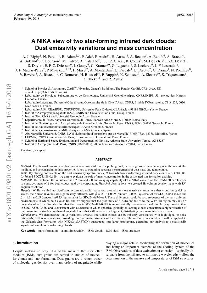
Fig. 6. Residuals resulting from the subtraction of the ratio maps con-volved using Gaussian kernels alone (RG) from the ratio maps con-volved using the PSF-matching technique (RP).

Fig. 7. The MAGPIS 20 cm continuum image of SDC18 at its native 6′′resolution. The contours show the 2.0 mm emission as in Fig. 5.

wavebands. The SDC24 field, by contrast, does not host any de-tectable 20 cm continuum emission in the MAGPIS image. The20 cm MAGPIS image of the SDC18 region is displayed in Fig.7 at its native resolution, with the 2.0 mm emission overlaid asblack contours. Diffuse emission can be seen across the wholeregion, but the morphology of the 2.0 mm peak to the east ofthe image – region C – matches the 20 cm continuum emissionvery closely indeed, indicating a source of contamination that islikely to dominate in that region. The 20 cm emission in regionsA and B does not correlate particularly well with the contoursof the 2.0 mm NIKA emission, suggesting that they are unre-lated and that any free–free contamination in the 2.0 mm band isminimal. We note that in these regions, the 1.2 mm and 2.0 mmmorphologies are very similar to each other, which adds weightto an origin in thermal dust emission. There is an exception tothe northwest of region A, where 20 cm emission does appear atthe edge of the 2.0 mm contours, and the 2.0 mm morphologydoes differ slightly from the 1.2 mm image.

We are unable to characterise the SED of the contaminatingregion (which we explore in more detail in Appendix A), but insummary we find that a significant proportion of the emissionin region C of SDC18 (see Fig. 5) may have arisen from free–free emission associated with the W39 H ii region, but do notfind convincing evidence that such contamination is significantin regions A and B. We also find that contamination from CO(2−1) emission is very small, and is present only at the levelof ∼ 1 − 3% across the region, though we are currently unableto measure this at any better than 50′′ angular resolution. SeeAppendix A for more details on our calculation of the CO linecontamination.



3.4. β maps

The combination of the 1.2 mm and 2.0 mm NIKA data allowsus to constrain the dust emissivity spectral index. This can bedone by computing the 1.2 mm to 2.0 mm intensity ratio, I1/I2.This ratio relates to β and Td through:

β = ln(

I1

I2

B2(Td)B1(Td)

)×

[ln

(ν1

ν2

)]−1

, (4)

which assumes a single average β and Td along the line-of-sight.The dust temperatures were determined through the SED fittingof the main clumps – presented in Sect. 3.1 – and are takenas Td = 14.32 ± 1.36 K in SDC18 and Td = 14.15 ± 1.32 Kin SDC24. At 1.2 mm and 2.0 mm, β only marginally dependson the temperature as the Rayleigh-Jeans regime is approached,meaning that the ratio I1/I2 is a good proxy for evaluating thevariations of β. However, the assumption of a single dust temper-ature throughout these IRDCs is simplistic, particularly whereembedded objects may be found, and we consider what biaseswe may thereby introduce later in this Section.

In Fig. 8, maps of β are displayed alongside histograms ofthe pixel values and with the corresponding uncertainty maps.In the case of SDC18, the free–free contamination that afflictedthe intensity ratios results in an even greater contrast betweenhigh- and low-β pixels. The frequency distribution peaks in the2.1 < β ≤ 2.2 bin, with a global mean of 1.83 and a stan-dard deviation of 0.70 though, as was the case with the inten-sity ratio maps, the three regions contribute different underlingpeaks to the overall distribution. The distribution spans the range−0.37 < β < 3.50 though it is likely that much of the low-β tailis a result of the free-free contamination which appears to bepresent in the eastern emission region that lies directly on top ofthe 20 cm continuum emission region. There appears to be a βgradient across the brightest clump (region A) in SDC18, thoughthese appear to be orientated in a similar direction to the 20 cmcontinuum emission visible in Fig. 7, and consequently may notgenuinely be present in that clump.

The SDC24 field, on the other hand, is clear of 20 cm contin-uum emission and so we can have confidence that free-free con-tamination is not a significant issue here. The β map of SDC24shows a lot of structure. Most of the extreme values are on theedge of the identified region where the S/N is lowest. The β valueis approximately 1.65 at the peak of the 2.0 mm emission, andit appears to rise moving out from the centre for a period, be-fore dropping again as the 2.0 mm intensity drops away. This isnot azimuthally constant, and there appears to be a difference to-wards the south of the clump where β becomes very high in oneparticular sector. Variations can also be seen towards the north-east, where a shoulder of 2.0 mm emission between the 3σ and20σ levels contains a β minimum. The frequency distribution ofβ values peaks at approximately ∼ 1.7, with a global mean of1.72 and a standard deviation of 0.34. This is consistent with thevalue of β = 1.89 ± 0.18 derived from the SED fit to the mainclump, though the latter represents an average within a 25′′ ra-dius of its centre.

As an internal consistency check, we compared β values de-rived from our β maps to the values recovered from the initialSED-fitting from Sect. 3.1 from which we derived our originaldust temperatures. In SDC18, using the same 25′′ aperture as forthe SED fit, we measured a mean β of 2.23, or a value of 2.11when each pixel value was weighted by 2.0 mm emission at thesame resolution (the latter being more directly comparable to theSED fit value). For SDC24, we obtained a mean aperture value

of 1.77 in the non-weighted case, and 1.73 when weighted bythe 2.0 mm emission. In both cases, the β values derived fromthe NIKA ratio maps lie within the uncertainty of the values re-covered from the SED-fits, though we note that in both cases, theNIKA ratio method recovers lower values.

Bracco et al. (2017) found systematic variations of β as afunction of radius in the vicinity of two protostellar cores in theTaurus B213 filament, with low values (β ∼ 1) towards the cen-tre, and increasing towards a value at larger radii that is con-sistent with the measurement in a pre-stellar core in the samefilament. We looked for similar systematic variations in SDC18and SDC24 by constructing radial profiles of β using annularapertures on the 20′′-resolution β maps of Fig. 8, centred on co-ordinates of the peak 1.2 emission, which we present in Fig.9. The annuli had a width of 3 arcseconds and measurementswere made out to a maximum radius of 40′′ from the peak of the1.2 mm emission. The error bars show the mean uncertainty ineach annulus resulting from error propagation (effectively aper-ture photometry on the ∆β map of Fig. 8), while the shaded re-gions indicate the standard deviations of the pixels in each annu-lus, disentangling the random and systematic components. Thestandard deviation in each annulus is the combined effect of bothrandom uncertainties, and intrinsic variations in β.

In both cases, the radial variations are small when comparedto the uncertainties that are dominated at small radii by the cal-ibration uncertainties, while at large radii by noise effects beginto increase the uncertainty. The variation in the outer annuli mayalso contain genuine variations in dust properties, but we are notsensitive to them using this technique and, in the case of SDC18,while the central ∼25–30′′are relatively free from free-free con-tamination (see Fig. 7), that contamination may have an effectin the outermost annulus. Future studies may improve on this if,for example, Hi-GAL data can be processed through the NIKApipeline to ensure that equivalent filtering is applied, and vari-ations in β could thereby be studied using pixel-by-pixel SEDfitting techniques, as used in the JCMT Gould Belt Survey’sSCUBA-2 studies (e.g. Sadavoy et al. 2013; Chen et al. 2016).The mean values, weighted by 1/σ2

i , where σi is the total uncer-tainty corresponding to each annulus, are β = 2.07 ± 0.09 andβ = 1.71 ± 0.09 for SDC18 and SDC24, respectively.

In constructing these β maps, we made the assumption that asingle dust temperature applies over the whole of each IRDC, de-termined from SED fitting in Sect. 3.1, though this is unlikely tobe the case in reality. We calculated additional β profiles for thetwo IRDCs using dust temperature maps generated using sev-eral different techniques, which are shown alongside the blue-circle fixed-temperature profile in the bottom panels of Fig. 9.The red crosses adopt dust temperatures from maps created us-ing a pixel-by-pixel SED fit using four Hi-GAL images at 160,250, 350 and 500 µm. The green stars adopt a temperature mapusing SED-fitting to Hi-GAL wavelengths again, but this timeadopting a fixed β of 1.8. Both β profiles generated using thetemperature maps from Hi-GAL SED fitting show almost iden-tical results, though we note that these temperature maps have anangular resolution of 40′′, a factor of two lower than our NIKAratio maps. Finally, the magenta triangles use colour tempera-ture maps created following Peretto et al. (2016), who demon-strated that the 160 µm and 250 µm Herschel imaging can beused to estimate dust temperatures at a resolution of . 20′′. Weconstructed the 160/250 µm ratio map by using the convolutionkernels of Gordon et al. (2008) to account for the non-Gaussianfeatures in PACS and SPIRE beams. This method requires theassumption of a value of the β, though the apparent circularityin this argument is mitigated by the fact that with the 160 µm



Fig. 8. Maps of the dust emissivity spectral index β for SDC18 (top row) and SDC24 (bottom row) with the corresponding histograms in the centralcolumn, and the associated total uncertainty maps (including both random and systematic contributions) in the right column. The black contoursshow the 2.0 mm emission as in Fig. 1, while the white contours show where the 1.2 mm S/N is equal to 25, above which we can expect therandom contribution of the noise to the value of β to be ∆β < 0.1. The 20′′ effective beam sizes are shown for scale.

0 5 10 15 20 25 30 35 40Radius [arcsec]

1.0

1.2

1.4

1.6

1.8

2.0

2.2

2.4

2.6

2.8SDC18

0.1 pc

Td: SEDTd: SED = 1.8Tc: 160/250 = 1.8Td = 14.3 ± 1.4 K

0 5 10 15 20 25 30 35 40Radius [arcsec]

1.0

1.2

1.4

1.6

1.8

2.0

2.2

2.4

2.6

2.8SDC24

0.1 pc

Td: SEDTd: SED = 1.8Tc: 160/250 = 1.8Td = 14.2 ± 1.3 K

Fig. 9. Radial profiles of β measured in SDC18 and SDC24. In each case, the blue lines show the mean value of β in the annuli centred on eachpoint, and the shaded blue regions show the standard deviation of pixel values within the corresponding annulus. The error bars combine theuncertainties from calibration, noise and temperature uncertainty. The solid black line at a radius of 10 arcseconds shows the extent of the effectivebeam. The profiles shown as red crosses, green stars and magenta triangles arise from adoption of the different temperature maps used as describedin Section 3.4.

to 250 µm intensity ratio, the wavelengths are close to the peakof the dust SED and thus relatively insensitive to β in the sameway that the 1.2 mm to 2.0 mm intensity ratio – far out in the tailof the SED approaching the Rayleigh-Jeans limit – is relativelyinsensitive to dust temperature. Comparison of profiles made us-ing β = 1.6 to profiles made using β = 2.0 leads to differences indust temperature of ∼1 K. In general, the effect of these varyingtemperature maps on the β profiles is very small, resulting onlyin small offsets of around ∆β .0.1 – much smaller than the errorbars. The biggest effect arises from the 160/250 µm ratio-deriveddust temperatures which are arguably the least robust. In fact, therelative insensitivity of the NIKA intensity ratio-derived β map

means that only implausibly high dust temperatures could yielda significant deviation.

4. Mass concentration

4.1. Column density maps

Column density maps from Herschel data can be calculated indifferent ways. The standard way is to perform a four-point (from160 to 500 µm) pixel-by-pixel SED fitting. For this, all data mustfirst be smoothed to a common angular resolution of, for exam-ple, 40′′, slightly larger than the original 36 ′′-resolution 500 µmimage to smooth any artefacts resulting from the data reduction



Fig. 10. Column density maps for SDC18 (left column) and SDC24(right column), calculated assuming a single β value in each IRDC. Themaps on the top row were generated by smoothing Hi-GAL imagingto a common resolution of 40′′, while those on the bottom utilise themulti-resolution technique, sampling between 40′′ and 13′′ to combineboth Herschel and NIKA data. The SDC18 contours show column den-sities levels of 2.0, 3.5, 5.0, 8.0, 12.0, 17.0 and 23.0 ×1022 cm−2, andthe SDC24 are the same with an additional contour at 1.5 ×1022 cm−2.Scale bars showing a 1 pc distance are displayed in the top left of eachpanel.

procedure as well as noise features. A modified black-body func-tion can then be fitted to the four data points at each position inthe map.

As we have seen in the previous Section, β does not vary sig-nificantly across each IRDC and so we adopted a fixed value forthe dust emissivity spectral index of β = 2.07 in SDC18 and β =1.71 in SDC24; these values are taken from the weighted meanvalues and lie within 3σ the Galactic average of β = 1.8 ± 0.2as measured by Planck (Planck Collaboration XXV 2011). Asin Sect. 3.1, we used the scipy.optimize χ2-minimisation routinecurve_fit to constrain the two remaining free parameters, NH2

and Td, thereby constructing both column density and tempera-ture maps at 40′′ resolution. The corresponding column densitymaps are displayed in the top row of Fig. 10. These images showthat the dust emission in both IRDCs is dominated by one source,and all compact sources that can be seen in the NIKA images inFig. 1 are blurred.

Higher-resolution column density maps can be obtained inseveral ways by making a few assumptions. The pixel-by-pixelSED-fitting procedure can be repeated with the exclusion of the500 µm point, carrying out a three point SED fit. Even though thefit is less well-constrained as a result of the decreased number ofdata points, with two free parameters and therefore one degreeof freedom, performing such a fit is still valid, and one can makesignificant gains in angular resolution, going from 40′′ to 27′′resolution (the raw 350 µm angular resolution is 25′′). Anotherway to construct column density maps is to calculate a colourtemperature using the 160 µm and 250 µm emission, and useEquation 2 to combine the resulting temperature map with the250 µm image to obtain a 20′′ column density image (e.g. Perettoet al. 2016). In each of these stages, column density maps areobtained using Herschel data alone.

Following Hill et al. (2012) and Palmeirim et al. (2013) itis possible to combine higher-resolution ground-based data with

Herschel observations to construct a column density image inwhich all the information at each wavelength is preserved. Theidea is that the four point SED column density map, N40′′

H2, is the

most reliable map for scales beyond 40′′, while the two higherresolution maps, N27′′

H2and N20′′

H2, provide additional information

on scale ranges [40′′ − 27′′] and [27′′ − 20′′], respectively. Thetilde here signifies that due to the way they have been constructed(i.e. with only a subset of the available data) these column den-sity maps are missing information on large scales. We can con-struct a fourth column density image, N13′′

H2, using the NIKA 1.2

mm image in a similar way as for N20′′

H2, using the same temper-

ature map (at 20′′ resolution). The following image can then beconstructed:

f l−sH2

= N sH2− N s

H2∗Gl, (5)

which includes the features on spatial scale range [l − s] to beadded to N l

H2in order to recover the N s

H2column density map.

The Gl term corresponds to a Gaussian kernel required to smooththe data to an angular resolution l. We can finally obtain an ex-pression for a column density map N13′′

H2at 13′′ angular resolu-

tion that includes all information at all scales using the followingequation:

N13′′

H2= N40′′

H2+ f 40′′−27′′

H2+ f 27′′−20′′

H2+ f 20′′−13′′

H2. (6)

The fact that spatial frequencies on arcminute scales havebeen filtered out of the NIKA data does not matter since we onlyretain features between 13′′ and 20′′ of the N13′′

H2column den-

sity image. We produced 13′′ column density maps in this way,and the resulting images are displayed in the bottom row of Fig.10. We can see that we have recovered many more structurescompared to the 40′′ column density map. In particular, we cansee the presence of several cores in the SDC18 that are not dis-cernible in the 40′′ map, while SDC24 remains dominated by asingle clump. Filamentary structures can be seen in SDC18 thatcorrespond with features in the 8 µm absorption of Fig. 1, thoughthe same can not be said for SDC24 for which the finer structuresremain unresolved. We remind the reader that for SDC18, thestructure to the east of the image at least (referred to as regionC in Figs. 5 and 8), is suspected to have arisen from free-freecontamination, and is probably not an authentic dust structure.

The various assumptions required to produce the 13′′-resolution column density map, N13′′

H2, means that it is intrinsi-

cally less accurate than the column density map N40′′

H2. To test

the magnitude of this difference, we smoothed the N13′′

H2using a

Gaussian kernel of FWHM 37.8′′ back to the original 40′′, andconstruct maps of the ratio of the smoothed N13′′

H2to the N40′′

H2

map. The distributions of pixel values in these column densityratio maps for SDC18 and SDC24, peak at 1.002 and 1.003 andwith standard deviations of 0.006 and 0.007, respectively. Thehigh-resolution column density maps contain 0.2−0.3% moremass in total, when compared to the more robust low-resolutionmaps, and pixel-to-pixel variations are on the order of 0.5%, giv-ing us a high level of confidence in this methodology. In the anal-ysis that follows from the combined N13′′

H2map, we have adopted

uncertainties derived from a corresponding error map, in whichthe uncertainties arising from the absolute calibration of the Her-schel and NIKA data have been propagated through each of theconstituent stages given in Eq. 6.



Table 3. Parameters used in the astrodendro analysis.

Source min_value min_delta min_npix

SDC18 3.5 × 1022 cm−2 0.1 × 1022 cm−2 24SDC24 1.5 × 1022 cm−2 0.1 × 1022 cm−2 24

4.2. Mass determination

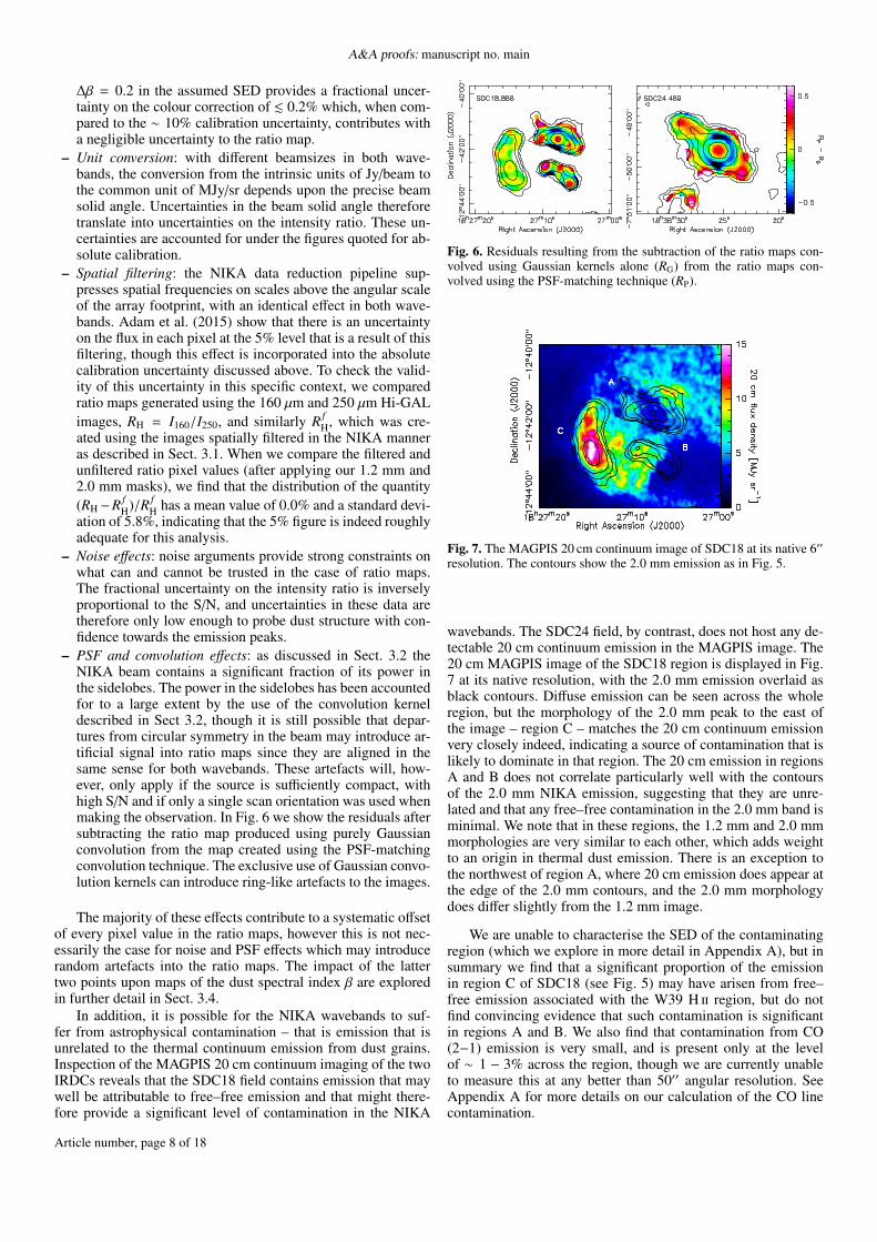
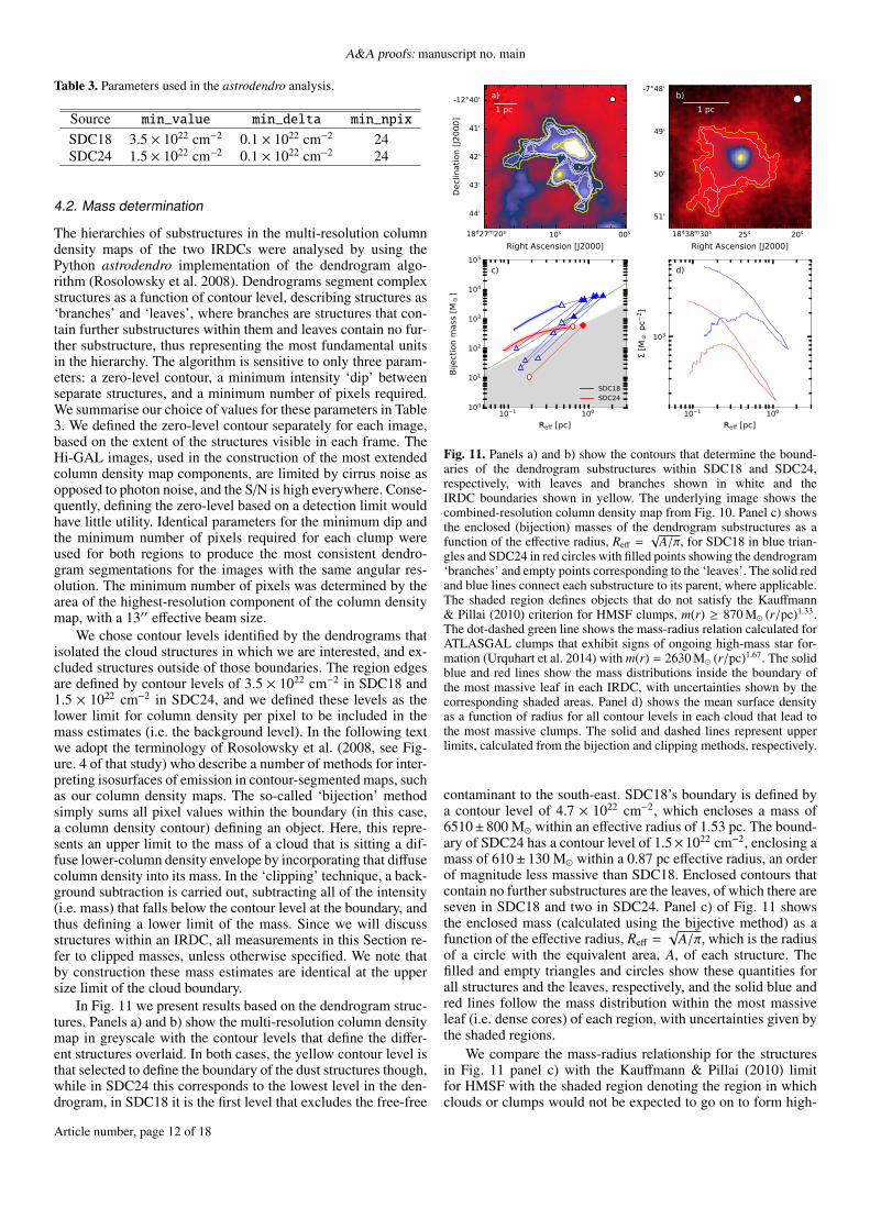
The hierarchies of substructures in the multi-resolution columndensity maps of the two IRDCs were analysed by using thePython astrodendro implementation of the dendrogram algo-rithm (Rosolowsky et al. 2008). Dendrograms segment complexstructures as a function of contour level, describing structures as‘branches’ and ‘leaves’, where branches are structures that con-tain further substructures within them and leaves contain no fur-ther substructure, thus representing the most fundamental unitsin the hierarchy. The algorithm is sensitive to only three param-eters: a zero-level contour, a minimum intensity ‘dip’ betweenseparate structures, and a minimum number of pixels required.We summarise our choice of values for these parameters in Table3. We defined the zero-level contour separately for each image,based on the extent of the structures visible in each frame. TheHi-GAL images, used in the construction of the most extendedcolumn density map components, are limited by cirrus noise asopposed to photon noise, and the S/N is high everywhere. Conse-quently, defining the zero-level based on a detection limit wouldhave little utility. Identical parameters for the minimum dip andthe minimum number of pixels required for each clump wereused for both regions to produce the most consistent dendro-gram segmentations for the images with the same angular res-olution. The minimum number of pixels was determined by thearea of the highest-resolution component of the column densitymap, with a 13′′ effective beam size.

We chose contour levels identified by the dendrograms thatisolated the cloud structures in which we are interested, and ex-cluded structures outside of those boundaries. The region edgesare defined by contour levels of 3.5 × 1022 cm−2 in SDC18 and1.5 × 1022 cm−2 in SDC24, and we defined these levels as thelower limit for column density per pixel to be included in themass estimates (i.e. the background level). In the following textwe adopt the terminology of Rosolowsky et al. (2008, see Fig-ure. 4 of that study) who describe a number of methods for inter-preting isosurfaces of emission in contour-segmented maps, suchas our column density maps. The so-called ‘bijection’ methodsimply sums all pixel values within the boundary (in this case,a column density contour) defining an object. Here, this repre-sents an upper limit to the mass of a cloud that is sitting a dif-fuse lower-column density envelope by incorporating that diffusecolumn density into its mass. In the ‘clipping’ technique, a back-ground subtraction is carried out, subtracting all of the intensity(i.e. mass) that falls below the contour level at the boundary, andthus defining a lower limit of the mass. Since we will discussstructures within an IRDC, all measurements in this Section re-fer to clipped masses, unless otherwise specified. We note thatby construction these mass estimates are identical at the uppersize limit of the cloud boundary.

In Fig. 11 we present results based on the dendrogram struc-tures. Panels a) and b) show the multi-resolution column densitymap in greyscale with the contour levels that define the differ-ent structures overlaid. In both cases, the yellow contour level isthat selected to define the boundary of the dust structures though,while in SDC24 this corresponds to the lowest level in the den-drogram, in SDC18 it is the first level that excludes the free-free

a)1 pc

18d27m20s 10s 00s

-12°40'

41'

42'

43'

44'

Right Ascension [J2000]

Decli

natio

n [J2

000]

b)1 pc

18d38m30s 25s 20s

-7°48'

49'

50'

51'

Right Ascension [J2000]

10 1 100

Reff [pc]

100

101

102

103

104

105

Bije

ctio

n m

ass [

M]

c)

SDC18SDC24

10 1 100

Reff [pc]

103

[M p

c2 ]

d)

Fig. 11. Panels a) and b) show the contours that determine the bound-aries of the dendrogram substructures within SDC18 and SDC24,respectively, with leaves and branches shown in white and theIRDC boundaries shown in yellow. The underlying image shows thecombined-resolution column density map from Fig. 10. Panel c) showsthe enclosed (bijection) masses of the dendrogram substructures as afunction of the effective radius, Reff =

√A/π, for SDC18 in blue trian-

gles and SDC24 in red circles with filled points showing the dendrogram‘branches’ and empty points corresponding to the ‘leaves’. The solid redand blue lines connect each substructure to its parent, where applicable.The shaded region defines objects that do not satisfy the Kauffmann& Pillai (2010) criterion for HMSF clumps, m(r) ≥ 870 M (r/pc)1.33.The dot-dashed green line shows the mass-radius relation calculated forATLASGAL clumps that exhibit signs of ongoing high-mass star for-mation (Urquhart et al. 2014) with m(r) = 2630 M (r/pc)1.67. The solidblue and red lines show the mass distributions inside the boundary ofthe most massive leaf in each IRDC, with uncertainties shown by thecorresponding shaded areas. Panel d) shows the mean surface densityas a function of radius for all contour levels in each cloud that lead tothe most massive clumps. The solid and dashed lines represent upperlimits, calculated from the bijection and clipping methods, respectively.

contaminant to the south-east. SDC18’s boundary is defined bya contour level of 4.7 × 1022 cm−2, which encloses a mass of6510±800 M within an effective radius of 1.53 pc. The bound-ary of SDC24 has a contour level of 1.5×1022 cm−2, enclosing amass of 610± 130 M within a 0.87 pc effective radius, an orderof magnitude less massive than SDC18. Enclosed contours thatcontain no further substructures are the leaves, of which there areseven in SDC18 and two in SDC24. Panel c) of Fig. 11 showsthe enclosed mass (calculated using the bijective method) as afunction of the effective radius, Reff =

√A/π, which is the radius

of a circle with the equivalent area, A, of each structure. Thefilled and empty triangles and circles show these quantities forall structures and the leaves, respectively, and the solid blue andred lines follow the mass distribution within the most massiveleaf (i.e. dense cores) of each region, with uncertainties given bythe shaded regions.

We compare the mass-radius relationship for the structuresin Fig. 11 panel c) with the Kauffmann & Pillai (2010) limitfor HMSF with the shaded region denoting the region in whichclouds or clumps would not be expected to go on to form high-



10 1 100

Reff / Reff, max

10 2

10 1

100

Mas

s con

cent

ratio

n [M

/Mm

ax] a)

SDC18SDC24

0.0 0.2 0.4 0.6 0.8 1.0Reff / Reff, max

0.5

1.0

1.5

2.0

2.5

Aspe

ct ra

tio

b)

Fig. 12. a) the concentration of mass as a function of radius within thetwo IRDCs. The solid and dashed lines show the upper and lower limitson the mass, respectively, calculated as in panel d) of Fig. 11. b) theaspect ratio (as defined by Peretto & Fuller 2009) of each structure as afunction of the normalised effective radius.

mass stars. The dominant clumps in both IRDCs lie in the non-shaded region, satisfying this criterion for HMSF. We also notethat these mass profiles for both clouds seem to follow brokenpower laws (in the case of SDC18, the profile can be tracedback through its parent structures which are the solid trianglesat larger effective radii), indicating a change in the volume den-sity profile of these IRDCs – becoming flatter in the inner re-gion, at Reff & 0.5 pc in SDC18 and Reff & 0.3 pc in SDC24.We note that another three of the dendrogram leaves of SDC18also fall above the Kauffmann & Pillai (2010) relation, thoughwe stress that we therefore interpret these as HMSF ‘candidates’since such a criterion is not conclusive on its own.

In panel d) of Fig. 11, the surface density is explored as afunction of radius within the most massive clumps and we see aturnover at an effective radius of ∼ 0.5 pc in SDC18 and ∼ 0.3pc in SDC24. Outside of these radii, the gradients of the upper(solid, bijection) and lower (dashed, clipping) limits converge,but the picture gets more confusing inside. In both cases, themid-point of the limits would appear to more-or-less flatten off,indicating that the volumetric density is behaving approximatelyas ρ(r) ∝ r−1 in the inner part of the clouds, and falls off morerapidly at larger radii.

Following up on our discussion of the steepness of the den-sity profiles, we decided to compare the mass concentration ofboth IRDCs. Fig. 12 a) shows the normalised mass profiles forboth IRDCs (normalised both in radius and mass) starting fromthe lowest level in the IRDCs – the yellow boundaries in panelsa) and b) of Fig. 11 – and following all substructures leading tothe most massive clump of each IRDC. At contour levels higherthan the boundaries of the leaves, the dashed profiles becomeequivalent to the shaded solid lines in panel c) of Fig. 11. Inpanel a) of Fig. 12 we see that, despite being an order of mag-nitude less massive, SDC24 is about a factor of ∼ 2 more con-centrated than SDC18 at most (normalised) radii. We calculatedthe aspect ratio for each contour level, following the method ofPeretto & Fuller (2009, see their Appendix A for a full formu-lation), which takes the ratio of the mass-weighted rms extent inthe direction each of the major and minor principal axes of iner-tia. In panel b) of Fig. 12 we can see that, at each level, the massdistribution in SDC24 is much more circular (aspect ratio closeto 1), and SDC18 only converges to an aspect ratio of ∼ 1 as thecontour level reaches a single beam in size. Since these aspectratios were estimated from the 2D projections of these objects,these are lower limits on the 3D aspect ratios of these clouds,

and the difference between the two IRDCs could potentially bemuch larger than a factor of 2.

5. Discussion

5.1. Evolution of dust properties

The evolution of dust properties and the emissivity spectral in-dex β is a long-standing issue. Sadavoy et al. (2013) createdmaps of β by using pixel-by-pixel SED fitting technique tocombine Herschel PACS and SPIRE data at 160–500 µm withJCMT SCUBA-2 450 and 850 µm data, finding that the addi-tion of the long-wavelength SCUBA-2 data allows significantimprovements in the determinations of β and dust temperatureto be made. Variations have been observed in various differentdatasets, and all found an anti-correlation between dust temper-ature and β. The so-called Td−β degeneracy can result from noisewhen using χ2-minimisation SED-fitting methods, though thiseffect should be minimised by reducing datasets to include onlyareas with very high S/N. Despite this Td−β degeneracy, severalstudies have concluded that the measurement degeneracies arenot sufficient to account for the entirety of the anti-correlation(e.g. Planck Collaboration XXV 2011; Chen et al. 2016), andan intrinsic physical anti-correlation has also been measured inlaboratory experiments (e.g. Agladze et al. 1996).

We see no evidence of significant systematic radial variationsin the dust emissivity spectral index, β, within the two IRDCs inour maps generated from the ratio of the two NIKA wavebands,regardless of the dust temperature model we adopt. However,we do see a significant difference in the β value between theclouds. Since these two images were taken in the same night, wecan say that the absolute calibration is the same in both maps,and so they should have the same systematic offset. Taking ac-count of this, we can say that the weighted mean β values ofβ = 2.07 ± 0.09 in SDC18 and β = 1.71 ± 0.09 in SDC24 aresignificantly different, indicating that the different environmentsare affecting the dust properties on spatial scales of ∼ 1 pc atleast. The uncertainty in the absolute calibration of both mapsprevents us from telling whether β is being elevated relative tothe Galactic average of β ≈ 1.8 in one cloud or whether it isbeing suppressed in the other. Higher-than-average β values inSDC18 could be explained by its location in the vicinity of theW39 H ii region. We note that although we would expect raiseddust temperatures in such an environment, we recover similartemperatures in SDC18 to the quiescent environment of SDC24.The Td−β degeneracy is insufficient to explain this, as repeat-ing the SED fitting for SDC18 with dust temperatures raised to17 K or 20 K yields poor results. The raised β is, perhaps, bestexplained by shocked regions along the line of sight being incor-porated into the column-averaged measurement.

Since we cannot assume a correlation between the calibra-tion of NIKA wavebands, we cannot constrain the absolute valueof β any more accurately than to within ∆β ≈ 0.25 with NIKAdata alone (a figure which arises directly from the 11% and 9%uncertainties in I1 and I2), even with extremely good S/N and thenegligible uncertainties on the dust temperature at these wave-lengths. Calibration of the background levels of the NIKA datausing the low-resolution but space-based Planck observationsprovides a feasible route to calibrate NIKA maps absolutely. Rel-ative differences between β values can still be measured, thoughthe search for radial trends in β should, in future, be carried outon maps with either higher sensitivity or brighter sources thanwe have in this study. A relative uncertainty in the NIKA ratio-derived β maps of ∆β < 0.1 can be achieved over regions in



which we can achieve S/N& 25. Higher sensitivity observationsover larger areas using this technique do have the potential toallow a study of systematic variations as a function of environ-ment.

Recent Planck results do, however, allow use to place ourβ values into some additional context, and we compare our re-sults to the latest all-sky dust temperature and β maps derivedby Planck Collaboration Int. XLVIII (2016). The effective reso-lution of Planck is much coarser than NIKA in these maps, witha 5.0′ FWHM, and so neither IRDC is resolved. For SDC18, thePlanck map has a value of Td = 22.3±1.1 K and β = 1.82±0.09,at the location of the 1.2 mm emission peak, and for SDC24values of Td = 21.1 ± 1.6 K and β = 1.78 ± 0.15 are recov-ered. In both cases, the NIKA data recover dust temperatures thatare roughly 8 K lower than those derived from the Planck data,though the β values fall within the quoted total uncertainties. Thefact that we recover systematically lower temperatures for ourIRDCs is not surprising; the spatial filtering applied to ground-based data such as our NIKA images biases the emission towardscompact sources, and compact infrared-dark sources will also becooler than the surrounding ISM. In addition to the effect of thespatial filtering is the relative beam dilution, which is significantwhen comparing 20′′-resolution data to that at ∼5′, and this ef-fect is compounded by further line-of-sight averaging.

While we do see a marginal (∆β ∼ 0.1−0.3) increase in themean value of β out to a radius of ∼20′′ in both IRDCs, the mag-nitude of this increase is small when compared to the variationsin terms of the standard deviation of β values as a function ofradius. The error bars in Fig. 9 within a radius of ∼30′′ are dom-inated by a systematic calibration offset, whereas the random un-certainties are better represented by the shaded regions that showthe 1σ deviations from the mean (though this probably also in-cludes intrinsic variations in β) and so, while all of the radialvariations we see are consistent with a constant central value,we are still sensitive to relative radial variations. However, be-yond ∼30′′, noise effects begin to dominate as the S/N becomeslow, and the visible relative differences can not be trusted. The βstructure away from the emission peak in SDC24 visible in Fig.8 is not azimuthally constant about the emission peak, and weexplore how this structure might arise artificially in AppendixB. The locations of artificial structures arising through noise ef-fects should correlate with low S/N regions, which is not the casefor all of the variations in this IRDC, though we cannot excludethe possibility that some of these structures have arisen throughbeam asymmetries. The effects of such asymmetries are difficultto model, but their impact can be reduced when making the ob-servations by observing in such a way that the position angle ofthe beam pattern varies with respect to the source.

The SDC24 region hosts a bipolar molecular hydrogen out-flow (MHO) identified by Ioannidis & Froebrich (2012) usingobservations of the 1−0 S(1) line of H2 at 2.122 µm from theUnited Kingdom Infrared Telescope. The approximate size andorientation of these outflows have been overlaid as magenta ar-rows on the β map in Fig. 13, with the location of the candidatedriving source MHO 3240 (a YSO associated with the UKIDSSsource GPS 43851 0698063) shown as a white star. By creating βmaps of outflows in L1157 using 1.3 mm MAMBO data and 850µm SCUBA data, Gueth et al. (2003) found that β varied system-atically across protostellar and outflow environments, suggestingthat shocked regions may have smaller dust grains, or alteredgrain chemistry. They found that β had its lowest value of ∼ 1.5at the location of the centre of the protostar in their observations,and reaching its highest value of ∼ 3.0 in the shocked regions. InSDC24, we find a similar coincidence of this β behaviour, albeit

Fig. 13. β map for SDC24 overlaid with the location of MHO 3240 –the driving source candidate (white star) – associated with the molecu-lar hydrogen outflows (magenta arrows) identified by Ioannidis & Froe-brich (2012). The contours show the 2.0 mm S/N as in Fig. 5.

with an offset of ∆β ≈ 0.5. The candidate driving source MH3240 falls on a minimum in our β map, with a value of β ≈ 1.0,and a maximum value of β ≈ 2.5 is coincident with the tip of theIoannidis & Froebrich (2012) southern outflow. However, we donot see any dust emission which is obviously associated with theoutflow itself and we have insufficient evidence to definitivelyshow that these β variations are causally linked to the outflowsfrom MHO 3240. Observations of shock tracers such as NH3 orSiO could be acquired in the future for comparison with varia-tions in the β maps, and observations in, for example, CO (3−2)could identify any link between the molecular outflow and theIRDC.

In a recent study, adopting a similar techniques to this studywith NIKA data, Bracco et al. (2017) found that out of threelow-mass cores in the Taurus B213 filament, the two protostellarsources exhibited radially increasing β profiles while the thirdpre-stellar core showed no evidence of any systematic variationin β. With neither SDC18 nor SDC24 showing any significant ra-dial variations in our study, despite both being protostellar, howdoes this result fit into the combined picture with the Braccoet al. (2017) study? There are some important differences to con-sider because, although the angular scales measured are almostidentical, SDC18 and SDC24 are far more massive and distantthan the Taurus filament. At a distance of 140 pc, the 40′′ ex-tent of the radial profiles corresponds to . 0.03 pc (. 6000 au),while it corresponds to & 0.8 pc and & 0.6 pc at the distancesof SDC18 and SDC24, respectively. Assuming that β increasesradially with the slopes given in that study, we would not expectto be able to resolve such variation at the distances of SDC18and SDC24. In addition, we expect the column densities in thetwo IRDCs to be much higher than in the Taurus filament, mean-ing that line-of-sight averaging is more significant in the former.Chacón-Tanarro et al. (2017) were also unable to resolve β vari-ations using NIKA in the pre-stellar Taurus core L1544, eventhough their resolution matches that of Bracco et al. (2017).

5.2. Mass concentration

SDC18 and SDC24 are morphologically very different whenobserved at NIKA resolution, which can be seen on the high-angular resolution column density maps of Fig. 10. One strik-ing feature is the large number of compact sources of SDC18revealed in the NIKA images. By contrast, the column densitystructure in SDC24 is relatively simple, with a dominant centralclump surrounded by a plateau of more diffuse emission. The8 µm GLIMPSE image (see Fig. 1) shows that there is a morecomplex underlying filamentary structure below the spatial sen-



Fig. 14. Herschel 70 µm images of SDC18 (left) and SDC24 (right)from the Hi-GAL survey. Note the bright 70 µm sources at the locationsof the column density peaks. The contours show the 2.0 mm S/N as inFig. 5.

sitivity of the dust continuum data, but which must contain asmall amount of the mass when compared to the central clump.The morphology of these two IRDCs also differ by their aspectratios – cf. Fig. 12 b) – where SDC18 is more elongated andfilamentary than SDC24.

Fragmentation theories of gravitationally unstable cloudshave shown that there are key differences in the wavelength ofthe fastest growing mode of density perturbations depending onthe initial morphology of the cloud (Larson 1985). While forspherical clouds, density perturbations of the length scale of thecloud diameter grow the fastest, while for filaments, perturba-tions of only a fraction of the filament’s length develop morerapidly (Inutsuka & Miyama 1992; Clarke et al. 2016). As aconsequence, filamentary clouds will more easily fragment intomultiple cores than more spherical clouds that will concentratemost of their mass into a single fragment, naturally leading to alarger mass concentration. The differences we observe betweenSDC18 and SDC24 could therefore be explained by different ini-tial conditions regarding the morphology of their respective massreservoirs.

We could also envisage that the observed differences aredue to different cloud evolutionary stages. We could imaginethat SDC24 started off more filamentary (as SDC18) and thatas a result of gravitational contraction ended up more spherical.If this would be correct, then SDC24 should have been form-ing stars for many free-fall times and should host a rich clus-ter at its centre, as predicted by the recent models of Vázquez-Semadeni et al. (2017). At 8 µm there is no evidence of suchcluster, but we do notice that the column density peaks are wellmatched with a compact source seen at 70 µm in Fig. 14 (sourcesHIGALPB018.8888-0.4744 and HIGALPB024.4888-0.6914 inthe Molinari et al. (2016) catalogue) and 70 µm fluxes also ap-pear to be in excess compared to the SEDs of the cold clumpsin Fig. 3. Luminosity at 70 µm has been shown to correlate wellwith internal protostellar luminosity, Lint, (Dunham et al. 2008)according to:

Lint = 3.3 × 108 F0.9470

(d

140 pc

)2

L, (7)

where the 70 µm flux, F70, has units of ergs cm−2 s−1, and dis the distance to the source in parsecs. Using the 70 µm fluxesfrom the Molinari et al. (2016) catalogue, we estimated the lu-minosity of young stellar objects seen at 70 µm for both IRDCs,finding Lint = 1410 ± 170 L for SDC18 and 155 ± 18 L forSDC24. Therefore, at the zero order, SDC18 is forming a largernumber and/or more massive protostars than SDC24, validating

the evolution scenario. However, because SDC18 is more mas-sive, we would expect it to form more stars anyway. Once theluminosities are normalised by the cloud masses, we obtain thefollowing luminosity to mass ratios: Lint/M = 0.22±0.04 LM−1

for SDC18 and Lint/M = 0.25 ± 0.06 LM−1 for SDC24. The

similar L/M values suggest that in absolute terms, both cloudsare forming a comparable number of stars per unit mass of gas(assuming the same star formation efficiency applies in both re-gions), and would therefore seem to exclude the possibility ofdifferent evolutionary stages as the cause of the morphologicaldifferences between SDC18 and SDC24.

5.3. Future studies

We have shown that creating maps of the dust emissivity spectralindex, β, can be achieved with NIKA data with relatively highresolution and precision. The absolute calibration of NIKA data,however, presents the biggest challenge in terms of determiningthe absolute value of β, and improvement on this front couldallow variation from region-to-region to be studied.

NIKA was a pathfinder instrument, in service on the IRAM30-m telescope from 2010–2015, and its much larger succes-sor, NIKA2 (Adam, R. et al. 2018), has been recently com-missioned. Further studies into β variations will be carried outas part of the GASTON survey (Galactic Star Formation withNIKA2), a guaranteed-time large programme with NIKA2, andimprovements to the absolute calibration can be made by us-ing the low-resolution spaced-based imaging from Planck to de-fine the background levels. Part of this programme will include ahigh-sensitivity study of part of the Inner Galactic plane in a re-gion rich with high-mass star-forming clumps and giant molecu-lar filaments, allowing studies of both β and mass concentration,as in this paper, to be expanded to a much larger and uniformlyobserved sample.

6. Summary

We have used 1.2 mm and 2.0 mm imaging from NIKA on the30 m IRAM telescope to study two IRDCs from the catalogue ofPeretto & Fuller (2009), SDC18 and SDC24. While SDC24 liesin a quiescent region, we find that some of the 2.0 mm emissionin the SDC18 region may be heavily contaminated with free–free emission from the W39 H ii region, and we use the NIKAimaging in tandem with data from the Hi-GAL survey to deter-mine dust properties surrounding the most massive clumps inboth regions.

We have constructed maps of the dust emissivity spectral in-dex, β, from the ratio of the specific intensities in both NIKA2wavebands after convolving them to a common angular resolu-tion. We use a FFT-based PSF-matching procedure to match the1.2 mm NIKA PSF to the 2.0 mm PSF, finding that the tele-scope beam sidelobes, if not accounted for, can introduce arti-ficial structures into the β maps, particularly in the neighbour-hoods of bright compact sources. The weighted mean centralvalues for β in SDC18 and SDC24 are β = 2.07 ± 0.09 (ran-dom) ±0.25 (systematic) and β = 1.71 ± 0.09 (random) ±0.25(systematic), respectively. Although we find no evidence for sig-nificant systematic radial variations of β in the dust immediatelysurrounding the dense clumps in the centres of these two IRDCs,we note that sufficiently high S/N are achieved over very limitedareas, with radii . 0.3 pc. Deviations from the mean β value inSDC24 might be linked to molecular hydrogen outflows from anearby YSO, though we do not have sufficient evidence to make



a definite causal link. In addition, since the observations of bothsources were carried out on the same night, the same system-atic calibration offsets apply and the relative difference in thecentral β values are reliable and significant. We suggest that theelevated β value in SDC18 compared to SDC24 may be causedby its proximity to the W39 H ii region.

We have also studied the relative mass concentration withinthe two IRDCs using a dendrogram-based analysis on high-resolution (13′′) maps of the H2 column density. We find thatSDC24 is more centrally concentrated than SDC18, with ahigher fraction of its mass concentrated within smaller nor-malised radii and lower aspect ratios at all column density con-tour levels. Both IRDCs have the same protostellar luminosityper unit of mass, indicating that the morphological differencescan not simply be attributed to an age effect, whereby SDC24could have been undergoing gravitational collapse for longerthan SDC18. This evidence supports a more spherical initialstate for SDC24 than SDC18, with internal fragmentation occur-ring on longer timescales than global collapse, while the morefilamentary SDC18 may be more unstable to fragmentation onsmaller scales.

Future studies of high-mass IRDCs using the techniques de-scribed in this paper with NIKA’s successor, NIKA2, as part ofthe GASTON large programme, will allow relative variations inβ to be measured over larger areas. In addition, with the highersensitivities that will be achieved, we will be able to study themass concentration over a much larger sample of IRDCs, allow-ing more quantitative conclusions about their initial conditionsto be reached.Acknowledgements. We thank the anonymous referee for helpful commentswhich have improved the quality and clarity of this paper. A. J. R. would liketo thank the STFC for postdoctoral support under the consolidated grant num-ber ST/N000706/1. N. P. also wishes to acknowledge support under the aboveSTFC consolidated grant as well as further support from the STFC under grantnumber ST/M000893/1. We thank the Royal Society for providing computingresources under Research Grant number RG150741. We would like to thank theIRAM staff for their support during the campaigns. The NIKA dilution cryo-stat has been designed and built at the Institut Néel. In particular, we acknowl-edge the crucial contribution of the Cryogenics Group, and in particular GregoryGarde, Henri Rodenas, Jean Paul Leggeri, Philippe Camus. This work has beenpartially funded by the Foundation Nanoscience Grenoble, the LabEx FOCUSANR-11-LABX-0013 and the ANR under the contracts "MKIDS", "NIKA" andANR-15-CE31-0017. This work has benefited from the support of the EuropeanResearch Council Advanced Grant ORISTARS under the European Union’s Sev-enth Framework Programme (Grant Agreement no. 291294). We acknowledgefundings from the ENIGMASS French LabEx (R. A. and F. R.), the CNES post-doctoral fellowship program (R. A.), the CNES doctoral fellowship program(A. R.) and the FOCUS French LabEx doctoral fellowship program (A. R.).This research made use of astrodendro, a Python package to compute dendro-grams of Astronomical data (http://www.dendrograms.org/), as well as Astropy,a community-developed core Python package for astronomy (Astropy Collabo-ration et al. 2013), SciPy (Jones et al. 2001) and matplotlib (Hunter 2007). Thisresearch has also made use of the NASA Astrophysics Data System.

ReferencesAdam, R., Comis, B., Macías-Pérez, J.-F., et al. 2015, A&A, 576, A12Adam, R., Comis, B., Macías-Pérez, J. F., et al. 2014, A&A, 569, A66Adam, R., Adane, A., Ade, P. A. R., et al. 2018, A&A, 609, A115Agladze, N. I., Sievers, A. J., Jones, S. A., Burlitch, J. M., & Beckwith, S. V. W.

1996, ApJ, 462, 1026Aniano, G., Draine, B. T., Gordon, K. D., & Sandstrom, K. 2011, PASP, 123,

1218Astropy Collaboration, Robitaille, T. P., Tollerud, E. J., et al. 2013, A&A, 558,

A33Benjamin, R. A., Churchwell, E., Babler, B. L., et al. 2003, PASP, 115, 953Bernard, J.-P., Paradis, D., Marshall, D. J., et al. 2010, A&A, 518, L88Beuther, H., Bihr, S., Rugel, M., et al. 2016, A&A, 595, A32Bracco, A., Palmeirim, P., André, P., et al. 2017, A&A, 604, A52Bradley, L., Sipocz, B., Robitaille, T., et al. 2016, astropy/photutils: v0.3

Cambrésy, L., Boulanger, F., Lagache, G., & Stepnik, B. 2001, A&A, 375, 999Carey, S. J., Noriega-Crespo, A., Mizuno, D. R., et al. 2009, PASP, 121, 76Catalano, A., Calvo, M., Ponthieu, N., et al. 2014, A&A, 569, A9Chacón-Tanarro, A., Caselli, P., Bizzocchi, L., et al. 2017, A&A, 606, A142Chen, M. C.-Y., Di Francesco, J., Johnstone, D., et al. 2016, ApJ, 826, 95Clarke, S. D., Whitworth, A. P., & Hubber, D. A. 2016, MNRAS, 458, 319Csengeri, T., Weiss, A., Wyrowski, F., et al. 2016, A&A, 585, A104Cyganowski, C. J., Whitney, B. A., Holden, E., et al. 2008, AJ, 136, 2391Désert, F.-X., Macías-Pérez, J. F., Mayet, F., et al. 2008, A&A, 481, 411Drabek, E., Hatchell, J., Friberg, P., et al. 2012, MNRAS, 426, 23Dunham, M. M., Crapsi, A., Evans, II, N. J., et al. 2008, ApJS, 179, 249Dupac, X., Bernard, J.-P., Boudet, N., et al. 2003, A&A, 404, L11Gordon, K. D., Engelbracht, C. W., Rieke, G. H., et al. 2008, ApJ, 682, 336Griffin, M. J., Abergel, A., Abreu, A., et al. 2010, A&A, 518, L3Gueth, F., Bachiller, R., & Tafalla, M. 2003, A&A, 401, L5Helfand, D. J., Becker, R. H., White, R. L., Fallon, A., & Tuttle, S. 2006, AJ,

131, 2525Hill, T., André, P., Arzoumanian, D., et al. 2012, A&A, 548, L6Hunter, J. D. 2007, Computing in Science & Engineering, 9, 90Inutsuka, S.-I. & Miyama, S. M. 1992, ApJ, 388, 392Ioannidis, G. & Froebrich, D. 2012, MNRAS, 421, 3257Jackson, J. M., Rathborne, J. M., Shah, R. Y., et al. 2006, ApJS, 163, 145Jones, E., Oliphant, T., Peterson, P., et al. 2001, SciPy: Open source scientific

tools for PythonJuvela, M., Demyk, K., Doi, Y., et al. 2015, A&A, 584, A94Kauffmann, J. & Pillai, T. 2010, ApJ, 723, L7Kauffmann, J., Pillai, T., Shetty, R., Myers, P. C., & Goodman, A. A. 2010a, ApJ,

712, 1137Kauffmann, J., Pillai, T., Shetty, R., Myers, P. C., & Goodman, A. A. 2010b,

ApJ, 716, 433Kerton, C. R., Arvidsson, K., & Alexander, M. J. 2013, AJ, 145, 78Larson, R. B. 1985, MNRAS, 214, 379Mezger, P. G. & Henderson, A. P. 1967, ApJ, 147, 471Molinari, S., Schisano, E., Elia, D., et al. 2016, A&A, 591, A149Molinari, S., Swinyard, B., Bally, J., et al. 2010, PASP, 122, 314Monfardini, A., Benoit, A., Bideaud, A., et al. 2011, ApJS, 194, 24Monfardini, A., Swenson, L. J., Bideaud, A., et al. 2010, A&A, 521, A29Ormel, C. W., Min, M., Tielens, A. G. G. M., Dominik, C., & Paszun, D. 2011,

A&A, 532, A43Ossenkopf, V. & Henning, T. 1994, A&A, 291, 943Pagani, L., Steinacker, J., Bacmann, A., Stutz, A., & Henning, T. 2010, Science,

329, 1622Palmeirim, P., André, P., Kirk, J., et al. 2013, A&A, 550, A38Pattle, K., Ward-Thompson, D., Kirk, J. M., et al. 2015, MNRAS, 450, 1094Peñaloza, C. H., Clark, P. C., Glover, S. C. O., Shetty, R., & Klessen, R. S. 2017,

MNRAS, 465, 2277Peretto, N. & Fuller, G. A. 2009, A&A, 505, 405Peretto, N., Lenfestey, C., Fuller, G. A., et al. 2016, A&A, 590, A72Planck Collaboration Int. XLVIII. 2016, A&A, 596, A109Planck Collaboration XXV. 2011, A&A, 536, A25Poglitsch, A., Waelkens, C., Geis, N., et al. 2010, A&A, 518, L2Ponthieu, N., Grain, J., & Lagache, G. 2011, A&A, 535, A90Reid, M. J., Menten, K. M., Zheng, X. W., et al. 2009, ApJ, 700, 137Roman-Duval, J., Jackson, J. M., Heyer, M., Rathborne, J., & Simon, R. 2010,

ApJ, 723, 492Rosolowsky, E. W., Pineda, J. E., Kauffmann, J., & Goodman, A. A. 2008, ApJ,

679, 1338Ruppin, F., Adam, R., Comis, B., et al. 2017, A&A, 597, A110Sadavoy, S. I., Di Francesco, J., Johnstone, D., et al. 2013, ApJ, 767, 126Sadavoy, S. I., Stutz, A. M., Schnee, S., et al. 2016, A&A, 588, A30Schuller, F., Menten, K. M., Contreras, Y., et al. 2009, A&A, 504, 415Shetty, R., Kauffmann, J., Schnee, S., & Goodman, A. A. 2009, ApJ, 696, 676Simon, R., Jackson, J. M., Rathborne, J. M., & Chambers, E. T. 2006, ApJ, 639,

227Siringo, G., Kreysa, E., Kovács, A., et al. 2009, A&A, 497, 945Smith, M. W. L., Eales, S. A., Gomez, H. L., et al. 2012, ApJ, 756, 40Steinacker, J., Pagani, L., Bacmann, A., & Guieu, S. 2010, A&A, 511, A9Swinyard, B. M., Ade, P., Baluteau, J.-P., et al. 2010, A&A, 518, L4Traficante, A., Calzoletti, L., Veneziani, M., et al. 2011, MNRAS, 416, 2932Urquhart, J. S., Moore, T. J. T., Csengeri, T., et al. 2014, MNRAS, 443, 1555Vázquez-Semadeni, E., González-Samaniego, A., & Colín, P. 2017, MNRAS,

467, 1313Wilson, T. L., Rohlfs, K., & Huttemeister, S. 2012, Tools of Radio Astronomy,

5th edition (Springer)Wilson, T. L. & Rood, R. 1994, ARA&A, 32, 191Yang, M. & Phillips, T. 2007, ApJ, 662, 284Ysard, N., Abergel, A., Ristorcelli, I., et al. 2013, A&A, 559, A133


http://www.dendrograms.org/


Fig. A.1. Maps of the free–free contamination fraction at 1.2 mm and2.0 mm, derived from the 20 cm MAGPIS data assuming an opticallythin H ii region. The black contours overlaid are from the correspondingNIKA maps at 20 arcsec resolution, and identical to those displayed inFig. 5.

Appendix A: Sources of contamination

Appendix A.1: Free-free contamination

We modeled the 20 cm continuum emission as an optically thinH ii region, with an SED described by the power law relationS H ii(ν) ∝ ν−0.1 (e.g. Mezger & Henderson 1967; Wilson et al.2012), in order to estimate the level of contamination from the20 cm continuum emission in both NIKA bands. After smooth-ing the data to 20 arcsec resolution, the flux density was cal-culated for both NIKA bands at 1.2 mm and 2.0 mm. Maps ofthe ratios of the modelled H ii region flux density at 1.2 mm and2.0 mm to the flux density of the corresponding NIKA maps areshown in Fig. A.1. It can be seen that, while the brightest sourceto the north-west is contaminated at less than the 20% level inboth bands at its centre, the source to the east is dominated byfree–free emission, especially at 2.0 mm – so much so that itmay not be a dust continuum source at all. The contaminationfraction exceeds unity in many areas in the 2.0 mm image, in-dicating that we have overestimated the 2.0 mm flux from thefree–free emission and that the assumed SED is not describingthese observations particularly well. We did not, therefore, sub-tract the calculated contaminant flux from our NIKA images, butwe regard region C as free–free dominated for the purpose of thisstudy.

To fully account for the contamination, a better characteri-sation of the contaminant H ii region is necessary and, while theMAGPIS data have excellent angular resolution, we lack data atother radio wavelengths to properly constrain the SED of the H iiregion. For future studies, data from the H i/OH/Recombinationline survey of the inner Milky Way (THOR; Beuther et al. 2016)could be used to determine the nature of the 20 cm continuumemission (i.e. free-free vs. synchrotron emission), allowing thecontamination to be more accurately modelled at 20 arcsec res-olution and subtracted from the 1.2 mm and 2.0 mm imaging.Additional continuum imaging in, for example, the 6 cm bandwould ensure that H ii regions could also be caught in the opti-cally thin regimes, which will not necessarily be true at 20 cm.

Appendix A.2: Line contamination

There is also potential for contamination in our 1.2 mm NIKAimages from the 12CO (2−1) emission line at 230.538 GHz,which lies towards the low-frequency edge of the 1.2 mm band(see Figure 2. of Bracco et al. 2017). In their NIKA study,Bracco et al. (2017) found this contamination to be at the levelof ∼ 1% towards their target filament in Taurus by using archival

data from the Five College Radio Astronomical Observatory(FCRAO), and we expect a higher level of contamination giventhat our targets lie on the Inner Galactic plane. Since no archivalCO (2−1) data exists towards our targets, we estimated the levelof contamination in our data by using 13CO (1−0) data from theBoston University FCRAO Galactic Ring Survey (GRS Jacksonet al. 2006). The GRS data have an angular resolution of 46′′and so we smoothed both our 1.2 mm imaging and the GRS datato an effective angular resolution of 50′′, and integrated the GRScubes over the full velocity range of −5 to 135 km s−1 to generatemaps of integrated intensity in units of K km s−1, and reprojectedthem onto a pixel grid matching our observations.

Converting an integrated intensity map of 13CO (1−0) emis-sion into 12CO (2−1) requires a number of assumptions to bemade. In conditions of local thermodynamic equilibrium, a com-mon excitation temperature is shared between all CO isotopo-logues, and the ratio of brightness temperatures of the same ro-tational transition of 12CO and 13CO are related by:

Tb(12CO)Tb(13CO)

=1 − e−τ(12CO)

1 − e−τ(13CO), (A.1)

where the optical depths, τ, for each isotopologue are related bytheir abundance ratio:

τ(12CO) = a12/13 τ(13CO), (A.2)

where a12/13 is the ratio of the abundance of 12CO compared to13CO. Isotopic abundances are measured to change as a functionof Galactocentric distance, and we adopted abundance ratios ofa12/13 = 40 for SDC18 and a12/13 = 45 for SDC24, follow-ing the prescription of Wilson & Rood (1994). We identifiedthe molecular cloud counterparts to SDC18 and SDC24 in thecatalogue of Roman-Duval et al. (2010) as G018.89-00.51 andG024.49-00.71, respectively, and by adopting the mean 13COoptical depths they derived for each cloud, we converted the13CO (1−0) integrated intensity maps to maps of integrated 12CO(1−0) intensity. We converted the maps of 12CO (1−0) into mapsof 12CO (2−1) by multiplying by a line ratio of R2−1/1−0 = 0.7,which is appropriate for cold, dense molecular gas (Peñalozaet al. 2017).

The GRS data contain no inherent filtering of spatial frequen-cies, since sky subtraction for spectral data is carried out by usingemission-free frequency channels. We therefore applied the 1.2mm NIKA transfer function (see Sect. 3.1 for a description of thetransfer function) to the GRS data to apply spatial filtering thatis equivalent to that applied to the NIKA continuum data, thusallowing the images to be compared directly. Finally, we fol-lowed the procedure of Drabek et al. (2012) to convert the mapsof 12CO (1−0) integrated intensity into units of mJy beam−1, byintegrating over the 1.2 mm NIKA bandpass, and thereby intoMJy sr−1 for direct comparison to our 1.2 mm images.

We found that the contamination is generally ∼ 1− 3%, withthe smaller values occurring with the peaks of 1.2 mm emission.CO (2−1) is likely to be optically thick for a Galactic plane clouddue to its relatively low critical density and so this contaminationwill be less important at areas of high column density. However,this contamination could become stronger at lower column den-sities, introducing a systematic bias as a function of column den-sity into the 1.2 mm to 2.0 mm intensity ratio as an extreme case.Although the angular resolution is necessarily reduced to 50′′ forthis test, we have seen no evidence that CO contamination is sig-nificant in our targets.



Fig. B.1. Synthetic β maps generated for two separate models: a) andb) are generated for a point source and c) and d) are generated for asource with a Gaussian intensity profile with a FWHM of 19 arcseconds.Panels a) and c) have been generated by convolution of the source witha Uranus beam map, while panels b) and d) were convolved with thebeam map after azimuthal averaging. The effective beam size is givenin the lower-right of panel d), and the contours represent S/N levels of3 and 25 from the 1.2 mm image.

Appendix B: Synthetic β maps

To determine what kind of artificial morphology might be intro-duced into the β maps as a consequence of noise and PSF effectswe created synthetic I1/I2 ratio maps for two source models: i)a perfect point-source and ii) a Gaussian source with a FWHMof 19′′, approximately equal to the deconvolved FWHM of themain clump in SDC24. To create synthetic 1.2 mm and 2.0 mmemission maps, each model was created on a 2′′ pixel grid andconvolved with a beam map (measured on Uranus and describedin Sect. 3.2) before Gaussian noise was added at the S/N levelmeasured for SDC24, listed in Table 2. These synthetic raw im-ages were then smoothed to an effective resolution of 20 arcsec-onds using the method described in Sect 3.2 before the 1.2 mmand 2.0 mm images were rescaled such that the ratio at the in-tensity peak corresponds to the ratio corresponding to β = 1.8and Td = 14.0 K according to Eq. 3. To explore the effects ofbeam asymmetries, a second synthetic observation was also pro-duced for both source models using the same noise realisationsat 1.2 mm and 2.0 mm, but differing in that the beam map wasazimuthally averaged before the beam convolution. After mask-ing to include only pixels with a S/N > 3 in both wavebands, thesynthetic observations were used to produce β maps assuming adust temperature of Td = 14.0 K, matching the input, so that theβ pixel values could be compared directly to the input value.

The four synthetic β maps are illustrated in Figure B.1, withversions created using the observed (asymmetric) beam mapas well as the azimuthally-averaged (symmetric) beam map foreach of the two source models. In all cases, the presence of noisehas introduced a host of synthetic features that deviate far fromthe input β value, with the most significant deviations at theedges of the maps. This would be expected as any coincidenceas any extrema in the noise in either or both wavebands could

translate into very large spurious deviations in their ratio aftersmoothing. To further constrain which regions of the β maps canbe trusted, an uncertainty map for the noise contribution to β canbe generated from the two S/N maps:

∆βnoise = 1.82

√1

(S/N)21

+1

(S/N)22

(B.1)

where (S/N)1 and (S/N)2 are the signal-to-noise ratios in the1.2 mm and 2.0 mm bands, respectively, and the numerical fac-tor is [ln (ν1/ν2)]−1. The accuracy to which β can be determined,based upon noise arguments alone and provided that a certainS/N has been achieved in both wavebands, can be describedby ∆βnoise = 2.57/(S/N); to restrict noise-based uncertaintiesto ∆βnoise = 0.1, we must look only at pixels for which theS/N is & 25 in both wavebands. The black contours in Fig.B.1 correspond to S/N of 3 and 25 for the synthetic 1.2 mmemission, and so we should expect to see noise-based deviationsof ∆βnoise < 0.1 within the top contour. This is approximatelytrue in the case of the models that used a circularly-symmetricbeam pattern, but more significant deviations can be seen in themore realistic asymmetric case, indicating that asymmetries inthe beam that may arise as a result of pointing or focus errorscan induce significant artificial structures.

Comparison of the artificial βmaps of Fig. B.1 with the mea-sured β maps of Fig. 8 then allows the measured structures tobe placed in some context. The white contour in Fig. 8 marksthe boundary above which the 1.2 mm S/N is greater than 25,where we can therefore expect to start detecting any significant∆β structures. The areas in the mapping where this criterion ismet are very limited, spanning only a slightly larger area thanone beam width and any underlying structure is certainly unre-solved. This comparison indicates that care should therefore betaken when interpreting features that fall below such a contourof S/N ∼ 25, though we should be confident in any variationsdetected above this level.
