Download - A new shared vehicle system for urban areas

Transportation Research Part C 21 (2012) 230–243

Contents lists available at SciVerse ScienceDirect

Transportation Research Part C

journal homepage: www.elsevier .com/locate / t rc

A new shared vehicle system for urban areas

Elvezia M. Cepolina ⇑, Alessandro FarinaDepartment of Civil Engineering, University of Pisa, Via Diotisalvi 2, 56126 Pisa, Italy

a r t i c l e i n f o a b s t r a c t

Article history:Received 19 January 2011Received in revised form 11 October 2011Accepted 14 October 2011

Keywords:Vehicle-sharing transport systemFleet dimension optimisationSimulated AnnealingSimulation

0968-090X/$ - see front matter � 2011 Elsevier Ltddoi:10.1016/j.trc.2011.10.005

⇑ Corresponding author. Tel.: +39 050 2217740; fE-mail address: [email protected] (E.M. Cep

The paper concerns the conceptual design of a transport system for pedestrian areas. Theproposed transport system is based on a fleet of eco-sustainable Personal Intelligent CityAccessible Vehicles (PICAVs). The vehicles are shared through the day by different usersand the following specific services will be provided: instant access, open ended reservationand one way trips. Referring to the proposed transport system, a new methodology to opti-mise the fleet dimension and its distribution among the stations is proposed in this paper.The problem faced is an optimisation problem where the cost function to be minimisedtakes into account both the transport system cost and the user costs that depend on thewaiting times. A random search algorithm has been adopted. Given a fleet dimensionand its distribution among the stations, the waiting times of the users are assessed by amicroscopic simulation. The simulation model tracks the second-by-second activity of eachPICAV user, as well as the second-by-second activity of each vehicle. The overall method-ology has been implemented in an object-oriented simulator. The proposed transport sys-tem has been planned and simulated for the historical city centre of Genoa, Italy.

� 2011 Elsevier Ltd. All rights reserved.

1. Introduction

The paper concerns a transport system, which would enable accessibility for all in urban pedestrian environments. Theresearch has been carried out within the PICAV project (DIMEC, 2009) founded by the European commission (SST-2008-RTD-1). The project’s aim is to design and build a new Personal Intelligent City Accessible Vehicle (PICAV) and to developa simulator capable of assessing how a homogeneous fleet of PICAV units would act as a transport system.

The PICAV unit is an electrically powered one person vehicle that will ensure accessibility for everybody and some of itsfeatures are specifically designed for people whose mobility is restricted for different reasons, particularly (but not only) el-derly and disabled people. Ergonomics, comfort, stability, assisted driving, eco-sustainability, parking and mobility dexterityas well as vehicle/infrastructures intelligent networking are the main drivers of PICAV design. The single units are networkedand can communicate each other, with city infrastructure, public transport on the surrounding area allowing high level ofinter-modal integration. Furthermore, it is capable of reducing its footprint and being driven in a standing position. The PI-CAV transport system is a multimodal shared use vehicle system for urban pedestrian environments. Stations are distributedat different locations through an area, and vehicle trips can be made between different stations. The PICAV vehicles can berented for a short time period (usually a couple of hours at a time and must always be returned by the end of the operatingtimes of a given day). The PICAV system gives people an alternative form of mobility in and around the historical city centre,where more traditional public transport services cannot operate because of the width and slope of the streets, uneven pave-ments and the interactions with high pedestrian flows. Thus, people can commute into the city and reach the border of thepedestrian area by traditional public transport, jump in a PICAV vehicle, visit attractions (shops, monuments, museums) in

. All rights reserved.

ax: +39 050 2217762.olina).

http://dx.doi.org/10.1016/j.trc.2011.10.005

mailto:[email protected]

http://dx.doi.org/10.1016/j.trc.2011.10.005

http://www.sciencedirect.com/science/journal/0968090X

http://www.elsevier.com/locate/trc

E.M. Cepolina, A. Farina / Transportation Research Part C 21 (2012) 230–243 231

the pedestrian area and drop the vehicle off at any PICAV station. Therefore, the PICAV transport system integrates into theexisting public transport system, adding a new efficient and rational service to citizens to access outdoor pedestrian envi-ronments which may have previously been inaccessible to them.

Characteristics of the PICAV transport system are: open-ended reservation system, instant access and one-way trips.The PICAV transport system has an on-demand, open-ended reservation system. It allows users to check-out a PICAV on

the spur of the moment, something that can occur at any time during system operation. Pure on-demand shared-use vehiclesystems (systems operating without any reservation capability) exist today (Shaheen and Cohen, 2007; Shaheen et al., 2006):for example, the UCR IntelliShare system has been operating for 3 years providing only on-demand service (Barth et al.,2000). On demand access to shared use vehicles provides much convenience to users; however, it places an additional bur-den on system management to satisfy user demand. In fact, reservations are useful for system management, allowing thesystem to maximise vehicle use thought the day. Furthermore knowledge of the travel demand, through reservations, makesit possible to estimate when a lack of vehicles may occur at any one station and then take corrective action (Barth et al.,2001).

Because one-way trips are allowed in a multiple station scenario, the number of shared use vehicles at each station canquickly become disproportionally distributed among stations. One way rental introduces significant flexibility for users butmanagement complexities, including necessitating vehicle relocation (Barth and Shaheen, 2003; Barth and Todd, 1999). Arelocation algorithm based on virtual spring forces has been proposed by Mukai and Watanabe (2005) where a controllerselects the car to be moved and station where it has to be moved. A stochastic optimisation method based on Monte Carlosampling has been proposed by Fan et al. (2008) to solve the car sharing dynamic vehicle allocation problem. Several relo-cation algorithms have been also developed by Barth and Todd (1999) and by Kek et al. (2006, 2009) to determine when andhow a relocation should occur in shared vehicle systems. An example of multiple station shared vehicle systems (MSSVS) isthe Praxitéle system being developed by a consortium of public transport operators, industrial manufactures and nationalresearch institutes in France (Augello et al., 1994). The Praxitéle system is based on small electric self-service vehicles thatare being applied to areas where traditional public transportation systems are not well adapted.

Therefore the PICAV transport system will provide high flexibility for users. However, in keeping with other MSSVS thesystem will be prone to becoming imbalanced with respect with the number of vehicles at the multiple stations. Due to un-even demand, some stations during the day may end up with an excess of vehicles whereas other stations may end up withnone. To solve this problem a fully user-based relocation strategy is proposed: a system supervisor is in charge of addressingat least part of the PICAV users (flexible users) to specific stations where they have to return the PICAV units.

This paper focuses on the problem of designing the fleet (i.e. its dimension and its distribution among the stations at thebeginning of the reference time period) for a given study area. The study area is described by a street network where stationsand ‘attractors’ (places where activities take place) are localised and by the PICAV transport demand. The PICAV transportdemand is defined by: how many PICAV users during the time period use the service; when and where do they require aPICAV unit; the characteristics of their trips by PICAV.

The optimal fleet is the one that minimises a cost function. The cost function takes into account the fleet cost and waitingtimes: both the terms are functions of the fleet dimension and the fleet distribution among the stations at the beginning ofthe reference time period. Since there is not an analytical expression for the cost function and the search space is extremelylarge, Simulated Annealing (SA) has been chosen for solving the minimisation problem. Given a PICAV fleet within the searchspace, the related cost function value is assessed by micro-simulation. This is achieved by inputting the street network, thePICAV transport demand and the PICAV fleet into the microscopic simulator, which then simulates the behaviour of thetransport system during the reference time period and assesses the waiting times of individual users.

The paper is organised as follows: Section 2 describes the proposed transport system. Section 3 outlines the fleet optimi-sation problem. Section 4 outlines the architecture of the transport system microscopic simulator. Section 5 describes therandom search algorithm then Section 6 describes the model implemented for the historical city centre in Genoa, Italy. Majorconclusions and future work follow.

2. The proposed transport system

We consider a sequence of time periods. A time period starts at 6.00 a.m. and ends at midnight and the sequence refers tosuccessive working days. We assume the rate of PICAV users that arrive in a given location on the urban pedestrian environ-ment border during a time period is the same in each period of the sequence as well as its distribution in time within theperiod. The characteristics of a PICAV user’s trip, in terms of destination, path, number of stops, stop locations and stop dura-tion, change randomly from one user to another but are the same for each user in the successive periods of the sequence.

We consider only visits to the urban pedestrian area during the reference time period, therefore the number of users whoenters the area during the reference time period equals the number of people who exits the area in the same time period.

If during a trip the PICAV user makes a stop that lasts more than 1 h, the PICAV unit will need to be parked in a station,which is referred to as ‘parking lot’ in this paper. If the stop duration is less than or equal to an hour short-term parking alongthe street is permitted and the PICAV unit does not need to be returned to a station.

In the area of study a number of parking lot sites have been identified. Trips by PICAV units begin (source) and end (sink)in these parking lots. The units are able to recharge when they are idle at the parking lots. Parking lots are conveniently

232 E.M. Cepolina, A. Farina / Transportation Research Part C 21 (2012) 230–243

placed in locations close to both inter-modal exchange points (like bus stops, underground stations, etc.) and attractors:points where activities that require long term stops take place (for instance museums, offices, schools). Each parking lot ischaracterised by what is called attractivity, which is a function of the places and things which attract people around the park-ing lot’s influence area.

The streets within the area of study are divided in sections. Each section is represented by a node and each node is char-acterised by an attractivity. The node’s attractivity is a function of the number and type of attractors within the related sec-tion. In this case attractors are places where a short term activity takes place (like food shops, cloth shops, handicraft shops).The user is allowed to park the PICAV unit along the street, not necessary in a station, for a period up to 1 h.

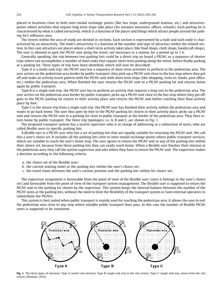
Generally speaking, the trip between two parking lots could be a direct trip on board a PICAV, or a sequence of shortertrips where one accomplishes a number of short tasks that require short term parking along the street, before finally parkingat a parking lot. Three types of trip have been identified, which will now be described:

Type A is a multi-task trip: the PICAV user has a sequence of short term activities to perform in the pedestrian area. Theuser arrives on the pedestrian area border by public transport, they pick-up a PICAV unit close to the bus stop where they gotoff and make an activity travel pattern with the PICAV unit with short term stops (like shopping, visits to: banks, post office,etc.) within the pedestrian area. When finished the user returns the PICAV unit to a PICAV parking lot and returns homeagain by public transport.

Type B is a single-task trip: the PICAV user has to perform an activity that requires a long rest in the pedestrian area. Theuser arrives on the pedestrian area border by public transport, picks-up a PICAV unit close to the bus stop where they got off,goes to the PICAV parking lot closest to their activity place and returns the PICAV unit before reaching their final activityplace by foot.

Type C is the return-trip from a single-task trip: the PICAV user has finished their activity within the pedestrian area andwants to go back home. The user thus goes by foot to the PICAV parking lot closest to their activity place, picks-up a PICAVunit and returns the PICAV unit to a parking lot close to public transport at the border of the pedestrian area. They then re-turn home by public transport. The three trip typologies, i.e. A, B and C, are shown in Fig. 1.

The proposed transport system has a system supervisor who is in charge of addressing at a subsection of users, who arecalled flexible users to specific parking lots.

A flexible user is a PICAV user who has a set of parking lots that are equally suitable for returning the PICAV unit. We callthis a user’s choice set. It includes all the parking lots close to inter-modal exchange points where public transport services,which are suitable to reach the user’s home stop. The user agrees to return the PICAV unit to any of the parking lots withintheir choice set, because from these parking lots they can easily reach home. When a flexible user finishes their mission inthe pedestrian area, they call the system supervisor and asks where they have to return the PICAV unit. The supervisor makesa decision according to the following criteria:

a. the choice set of the flexible user;b. the current waiting times at the parking lots within the user’s choice set;c. the travel times between the user’s current position and the parking lots within his choice set;

The supervisor assignment is favourable from the point of view of the flexible user (since it belongs to the user’s choiceset) and favourable from the point of view of the transport system management. The flexible user is supposed to return thePICAV unit to the parking lot chosen by the supervisor. This system keeps the internal balance between the number of thePICAV units at the parking lots, without the need to limit the flexibility of the transport system or have external operators toredistribute the PICAVs.

This system is best suited when public transport is mainly used for reaching the pedestrian area. It allows the user to exitthe pedestrian area close to any stop where suitable public transport lines pass. In this case the number of flexible PICAVusers is supposed to be consistent.

Fig. 1. The three types of missions: Type A (multi task mission), Type B (single task trip to the city centre), Type C (single task trip, return from the citycentre) (Bonfanti, 2010).


The paper proposes an optimisation algorithm which is able to assess the best number of PICAV units to assign to eachparking lot at the beginning of each time period. Only at the end of the time period (for instance during the night) an externaloperator is supposed to rebalance the PICAV units among the parking lots, in such a way to establish again the initial con-ditions at the beginning of the following time period. In the real world, the relocation of vehicles can occur either using alarge truck that can carry or tow several PICAV units, or by having the vehicle platoon under their own power.

3. Fleet dimension optimisation

The problem of assessing the best number of PICAV units to assign to each parking lot at the beginning of all the timeperiods of the sequence is formulated as a constrained minimisation problem. The function z to be minimised is a linear com-bination of the transport system cost Csystem

day and of the user’s costs Cusersday , subject to the constraint that the 90th percentile of the

waiting time t90%w is not bigger than the threshold of 5 min. Both the costs refer to the daily reference time period and their

units are €/day

min z ¼ minðCsystemday þ Cusers

day Þ subject to t90%w 6 5 ð3:1Þ

The transport system cost includes the cost Cfleetday of purchasing the fleet, the running cost Crunning

day of the PICAV units, thecost Csetup

day of the parking lots setup and the management costs Cmanagementday . The revenue Ctickets

day derived from the tickets is sub-tracted from Csystem

day

Csystemday ¼ Cfleet

day þ Crunningday þ Csetup

day þ Cmanagementday � Ctickets

day ð3:2Þ

For Cfleetday , we assume that each PICAV unit purchase price is 9000 €. This cost includes the vehicle with a lifetime of 8 years

and two lithium-ion battery packs with a lifetime of 4 years each. The cost of adding vehicles to the system increases linearlywith each vehicle. The linear increase in vehicle costs is a rather simplistic assumption and does not take into account anyeconomy of scale, however it is also a quite frequent assumption (Barth and Todd, 1999). The daily cost to amortize the fleetpurchase cost has been calculated with a discount rate of 8%, according with the following formula:

Cfleetday ¼ nvehcveh

rð1þ rÞlt

ð1þ rÞlt � 1

" #1

365ð3:3Þ

where nveh is the number of PICAV units within the fleet, cveh is each PICAV unit purchase cost (it includes two battery packs),r is the discount rate and lt (number of years) is the PICAV unit lifetime.

We chose a discount rate of 8% as it is an average rate of return for investments and thus reasonably represents the oppor-tunity cost of the purchase. There is disagreement on what should be the appropriate discount rate but it is a parameter inthe proposed methodology and a sensitivity analysis can be performed.

Crunningday includes the maintenance costs and the electricity cost to run the PICAV fleet. Referring to the maintenance costs, if

we exclude the expensive batteries that must be replaced since we already included them in the vehicle purchase cost, elec-tric cars incur very low costs and we neglect them. As it concerns the electricity needed to charge all the PICAV units duringan operative day, it is proportional to the average daily kilometres travelled by the PICAV users. Since we assume a constantPICAV transport demand, the average daily kilometres travelled by the PICAV users does not depend on the fleet dimension.Therefore, the electricity cost is represented as a flat cost.

Csetupday includes infrastructure cost that relates to the number of parking space in each lot. This cost depends on the fleet

dimension; however due to the small dimension of PICAV units (1.1 m long and 0.9 m wide) we considered it as a flat cost.Again Cmanagement

day , which includes the salaries of the system supervisor and of the external operator are flat costs. In fact,the proposed relocation strategy is fully user-based and the external operator is only in charge of the PICAV unit rebalance atthe end of the time period. Ctickets

day is the revenue derived from the tickets. Multiplying the number of PICAV users by ticketprice provides approximate ticket revenues. Since the number of PICAV users in a time period has been assumed constant,Ctickets

day is again a flat cost.With regards to the second term Cusers

day in 3.1, this has been measured in terms of the total customer waiting time and thecost the users have to pay for the service. The total customer waiting time is the overall length of time, in minutes, customershave to wait for a vehicle when a vehicle is not immediately available during the reference time period. Cusers

day has the follow-ing expression:

Cusersday ¼ cw

Xm

i¼1

twi þ Cticketsday ð3:4Þ

where cw is the cost of a unit of waiting time, namely 0.10 €/min (Cherchi, 2003), m is the total number of users who havebeen in a queue during the reference time period, twi is the waiting time of user i (min/day) which is a function of the numberof PICAV units assigned to each parking lot at the beginning of the time period,

Pmi¼1twi is the total customer waiting time in

the reference time period (min/day). It is a function of the number of PICAV units assigned to each parking lot at the begin-ning of the time period and Ctickets

day is the overall cost paid by the PICAV users and it is given multiplying the number of PICAVusers by ticket price. Since the PICAV transport demand has been assumed constant, Ctickets

day is again a flat cost. Moreover this


term equals the revenue derived from the tickets that appears in the transport system cost, therefore since both the termsappear in the cost function with opposite signs, and therefore delete each other.

If we call p a vector whose dimension is equal to the number of parking lots and the value of each vector componentequals the number of PICAV units in the related parking lot at the beginning of the reference time period, we have thatPm

i¼1twi is a function of p:Pm

i¼1twiðpÞ.Instead of minimising the z function in order to assess the best number of PICAV units to assign to each parking lot at the

beginning of the time period, we minimise another function f which is simply the function z but without the flat cost termssince they do not affect the minimisation problem. The f function has the following expression:

f ðpÞ ¼ nvehcvehrð1þ rÞlt

ð1þ rÞlt � 1

" #1

365þ cw

Xm

i¼1

twiðpÞ ð3:5Þ

In the formulated problem, the independent variable is p since nveh is the sum of all the p’s components. The search spaceis given by Na if a is the number of parking lots in the study area: therefore the research space could be extremely large.

We introduce a constraint on the f(p) minimisation problem: we want that the 90th percentile of the waiting time t90%w ðpÞ

to be less than a threshold of 5 min. Therefore we consider the f(p) minimisation problem with a single inequality constraintg(p) 6 0 where ðpÞ ¼ t90%

w ðpÞ � 5.We transform the constrained problem:

Minimise f ðpÞSubject to : gðpÞ 6 0

ð3:6Þ

into a single unconstrained problem using penalty functions. The constraint is placed into the objective function h(p) via apenalty parameter l̂ > 0 in a way that penalises any violation of the constraint:

Minimise hðpÞ ¼ f ðpÞ þ l̂½maximumf0; gðpÞg�2

Subject to : p 2 Na;where Na is the search space:ð3:7Þ

If g(p) 6 0, then the [maximum{0, g(p)}]2 = 0, and no penalty is incurred. On the other hand, if g(p) > 0, then [maxi-mum{0, g(p)}]2 > 0 and the penalty term l̂½maximumf0; gðpÞg�2 is applied.

The weight of the penalty function l̂ is unknown and we determine it with an iterative process, according with Bazaraaet al. (1993), starting from a small value and increasing it progressively. In fact, as the value of l increases, the optimal solu-tion of h(p) get arbitrarily close to the optimal solution of the original constrained problem: Minimise f(p) Subject to:g(p) 6 0. The initial value of the penalty parameter is taken as l1 = 0.1, and is updated as follows: lk+1 = blk, where the scalarb is taken as 10.0 and k and k + 1 are two successive iterations.

For a given lk, we have a function hk(p) to minimise. If the vector p� that minimise hk(p) is the same vector for whichg(p�) ffi 0 we stop the iterative process and l̂ ¼ lk.

For a given value for the penalty parameter lk and a given point in the research space (a given pp), we calculate the valueof the hk(pp) function simulating the transport system with the microscopic simulator that will be described in the followingsection. Given an area of study and the number of PICAV users, the simulation input is the PICAV fleet, represented by a givenvector pp, and the simulation outputs are the total customer waiting time

Pmi¼1twiðppÞ and t90%

w ðppÞ.Since there is no analytical expression for hk(p), we cannot exclude the need to deal with a multi-peak function and the

risk of reaching a local minimum, without being able to find the global minimum, is high. To combat this issue and the factthat the research space is extremely large, Simulated Annealing (SA) has been chosen to solve the minimisation problem.

Both the procedure for the assessment of hk(p) values and the one for solving the minimisation problem by the SimulatedAnnealing are described respectively in Sections 4 and 5.

4. The microscopic simulation model

The microscopic simulator simulates the behaviour of the transport system in a given time period. It allows one to trackthe second-by-second activity of each PICAV user, as well as the second-by-second activity of each vehicle. The simulator hasbeen written with Python 2.5 (Van Rossum, 2006) along with standard scientific computing package for Python (Numpy1.4.0). Python follows an object-orientated logic. The simulation model is event-driven.

4.1. The simulator components

4.1.1. The PICAV userEach PICAV user i is defined by:

– the initial condition Ci0 of each individual,– the activity-travel pattern of the individual in the urban area: (Ti, Li), where i refers to intermediate stops for Type A trips,– the destination choice set Di of the individual.


The initial condition Ci0 of an individual i is described by a vector (ti0, Li0) where: ti0 is the time of arrival and Li0 the loca-tion where the individual i arrives, which is always on the edge of the historical city centre.

The activity-travel pattern of an individual i, is composed of a series of activities (that require short-term stops), and tripsbetween these activities on a PICAV. The activity-travel pattern is described by: (Ti, Li) = (Ti1, . . . ,Tiz, . . . ,Tina; Li1, . . . ,Liz, . . . ,Lina),where: Tiz is the duration of the zth activity pursued by individual i; Liz is the location of the zth activity pursued by individuali, and na is the number of activities involved in individual i’s activity-travel pattern.

(Ti, Li) is never equal to (0, 0) for Type A trips. (Ti, Li) is equal to (0, 0) for Type B and Type C trips, since these trips aredirect trips between parking lots.

The destination choice set, Di = (PL1, . . . ,PLj, . . . ,PLncs) where PLj is a parking lot that is convenient for individual i and ncs isthe number of parking lots within the choice set:

– For Type B trips PLj is an attractor in the historical city centre, where activities that require a stop greater than 1 h takeplace. Therefore, ncs = 1 and the parking lot corresponds to the final destination Di = (DiF).

– For Types A and C trips PLj is an inter-modal exchange point, a place where individual i can transfer onto another form ofpublic transport to reach their home There is a choice of places, all with equal attractivity to the flexible user, thereforencs >1. The final destination DiF will be chosen within Di by the system supervisor.

4.1.2. The PICAV unitEach PICAV unit is characterised by: its initial parking lot, the charging time, the battery capacity and the battery dis-

charging law.

4.1.3. The PICAV parking lotParking lot PLj is characterised by: the number of PICAV units at the parking lot at the start of the simulation, by the park-

ing lot attractivity and by a vector (WPLj) representing the waiting times of users at the parking lot PLj. WPLj ¼ðtw1

PLjðtÞ; . . . ; twiPLjðtÞ; . . . ; twO

PLjðtÞÞ; where twiPLðtÞ, is the current waiting time of the ith PICAV user and O is the number of PI-

CAV users at the parking lot PLj at time t.

4.1.4. The transport system supervisorWhen a PICAV user i calls the transport system supervisor and asks which parking lot, they should return the PICAV unit

to, the system supervisor chooses the final parking lot DiF for the individual i according to the system state. The choice is afunction of:

– The user i’s choice set Di = (PL1, . . . ,PLj, . . . ,PLncs).– The current maximum waiting times at the parking lots belonging to the user’s choice set: ðtwMAX

PL1 ; :::;

twMAXPLj ; :::; tw

MAXPLncsÞ where twMAX

PLj ¼ max8individual i at PLj

ftwiPLjg8PLj 2 Di.

– The foreseen travel times ttiCj between the current user i’s position and the parking lots belonging to the user’s choice set

ðttiPL1; . . . ; tti

PLj; . . . ; ttiPLncsÞ where tti

PLj is the foreseen travel time between the user’s current position and the localisation ofPLj.

The system supervisor addresses the user to the final parking lot DiF which belongs to the user’s choice set. If there is atleast a user in queue in any of the parking lots belonging to the user’s choice set, DiF will be the parking lot for which the ratebetween the current maximum user’s waiting time and the foreseen travel time between the user’s current position and thelocalisation of the parking lot is maximum

if MAX8PLj2Di

ðtwMAXPLj Þ > 0

twMAXDiF

ttiDiF

¼ MAX8PLj2Di

twMAXPLj

ttiPLj

!ð4:1:aÞ

If there are no users in queue in any of the parking lots belonging to the user’s choice set, DiF will be the parking lot forwhich the product between the number of available vehicles at the parking lot at the current time instant (nva

PLj) and the fore-seen travel time between the user’s current position and the localisation of the parking lot is minimum

if MAX8PLj2Di

ðtwMAXPLj Þ ¼ 0 tti

DiF � nvaDIF ¼ MIN

8PLj2Di

ðttiPLj � nva

PLjÞ ð4:1:bÞ

4.2. The PICAV transport system microsimulator

The main steps of the simulator are briefly reported here:

� Firstly, PICAV users are generated at time ti0 and in parking lot PLj. The initial condition Ci0 of an individual i is a deter-ministic input: we assume the number of PICAV users that arrive in a given location on the area border during the timeperiod is known as well as its distribution in time within the period. Each PICAV user is generated with a type of trip


(Types A, B or C), their activity-travel pattern (Ti, Li) and choice set Di. The type of trip, activity-travel pattern and thechoice set are stochastically generated. The type of trip is assigned to the PICAV user i according to the probability of eachtype of trip occurring. The activity-travel pattern, Li depends on the nodes’ attractivities whilst Ti is assumed to be con-stant for all the activities.Di, depends on the type of trip assigned to the user. If the user has been generated with a Type A or Type C trip, Di isrelated to a macro-area at the edge of the area of interest. A macro-zone is a subdivision of the urban area outside thepedestrian zone and is characterised by a choice set. This includes all the parking lots close to public transport stops thatlink the macro-zone to the pedestrian area. Each macro-zone is also characterised by a weight that represents the per-centage of users that travel from the macro-zone to the pedestrian area border. We assign a macro-zone to each PICAVuser i according to the macro-zone’s weights and therefore we assign to the user the choice set related to the assignedmacro-zone. If the user has been generated with a Type B trip, Di is composed of only one parking lot (DiF) which isassigned to the user according to the parking lots’ attractivities.For each generated PICAV user i, the simulator adds a component to the PLj’s array of waiting times. If in the parking lotthere is a PICAV unit available, a PICAV unit is assigned to the individual i and the component related to their waiting timeis deleted from the parking lot’s array.� After creating the users and their journeys, the simulation of these travel patterns and the subsequent battery discharging

process for all PICAV units in use is completed.The transit time is calculated based on the trip distance and dividing by the maximum cruise speed of the PICAV vehicle.This is rather simplistic and in the future we would like to introduce a friction term that takes into account the interac-tions between a PICAV unit and pedestrian flows.For all the users who at the current simulation time complete the nath activity in their daily activity-travel pattern, theiractivity-travel pattern (Ti, Li) is set equal to (0, 0).For all users who at the current simulation time have (Ti, Li) = (0, 0) and Di = (PL1, . . . ,PLj, . . . ,PLncs) with ncs > 1, a call to thesystem supervisor is generated. A final parking lot DiF is assigned by the system supervisor to the user who called him.For all users that at the current simulation time have an assigned DiF, the time of travel between their current positionand the DiF along with the related battery discharging process are simulated.All the users that at the current simulation time arrive at the parking lot DiF are deleted from the simulation world. If theirPICAV unit battery charging level is low, the unit recharges itself while idle at the parking lot. These units are not availablefor hire during this recharging period. When the charging level is high, the PICAV unit becomes available to new users atthe parking lot.� The charging process for PICAV units at the parking lots. If at the current simulation time PICAV units have completed the

charging process, they become available for new users at the parking lot.� The assessment of the customer satisfaction measures at the end of the simulated time period: the total waiting time and

the waiting time of the 90th percentile are assessed. The first measure is computed by summing the waiting times of allthe PICAV users. The second measure is computed by dividing in classes the waiting times and by assessing the number ofusers whose waiting time falls into each class.

5. The Simulated Annealing

The Simulated Annealing scheme is a stochastic method currently in wide use for difficult optimisation problems. Sim-ulated Annealing is motivated by an analogy to annealing in solids searching for minimal energy states. This procedure heatsthe metal to a high temperature so that it is a liquid and the atoms can move relatively freely. The temperature of the metalis slowly lowered so that at each temperature the atoms can move enough to begin adopting the most stable orientation. Ifthe metal is cooled slowly enough, the atoms are able to ‘relax’ into the most stable orientation. This slow cooling process isknown as annealing and so the method is known as Simulated Annealing.

The method is an iterative process that searches from a single point moving in its neighbourhood and allows worse movesto be taken some of the time. Therefore, it could allow, for example, some uphill steps to be taken so that a local minimumcan be escaped. Worse solutions are accepted according to a probability. This probability depends on a parameter, i.e. thetemperature, which decreases with the number of steps.

The algorithm evolves by means of an iterative cycle, in which the search space is explored. This search depends on acontrol parameter called temperature T which decreases as the number of the iteration of the cycle increases. In each iter-ation, a new point Sn is reached from S, according to the transition rule. At the new point, the value of the cost function f ischecked. At each iteration, the following two variables are taken into account and updated:

– the generated new solution Sn;– the current solution S.

The updating happens according to:

(a) if f ðSnÞ 6 f ðSÞ ! Sn substitutes S: S: = Sn,(b) if f ðSnÞ > f ðSÞ ! Sn will become the current solution S with a probability given by:


p ¼ exp � f ðSnÞ � f ðSÞT

� �ð5:1Þ

This is the core of Simulated Annealing and is known as the Metropolis algorithm. T is the value of the temperature for thecurrent inner cycle (Laarhoven and Aarts, 1987).

Given that R e [0, 1] is an pseudo random number, updating happens according to the following:

if R 6 p ? the new solution Sn substitutes S.if R > p ? the new solution Sn is rejected and therefore S will not be updated.

Therefore the algorithm needs the definition of the cooling schedule, the local search and the starting and stoppingconditions.

5.1. The cooling schedule

The cooling schedule is defined by: the initial temperature, the law of its decrease and the final temperature. We fixed thecooling schedule in such a way as to guarantee a good exploration of the research space.

The starting temperature has been determined according to Laarhoven and Aarts (1987). An initial acceptance ratio p0 ofthe worse solution, e.g. 0.9, is fixed at the first step of the algorithm. From this point, the initial temperature T0 is determinedfrom the acceptance ratio p0 in this way:

0:9 ¼ p0 ¼ exp � f ðSnÞ � f ðSÞT0

� �ð5:2Þ

The most commonly used temperature reduction function is geometric: Tk+1 = a � Tk where Tk and Tk+1 are the temperaturesin two consecutive iterations of the algorithm (Laarhoven and Aarts, 1987). Typically, 0:7 6 a 6 0:95. A very slow coolingschedule has been adopted to guarantee a good exploration of the search space:

a ¼ 0:99 ð5:3Þ

The final temperature scheme of the cooling schedule is replaced by a stopping condition. The algorithm is stopped whena high number of iterations, i.e. 5000, is reached.

5.2. The transition rule

The generic point S of the search space coincides, in the problem faced in this paper, with the vector p described inSection 3.

The transition rule allows the exploration of the search space: from a given PICAV fleet, represented by a vector p, a newPICAV fleet pn is selected in the neighbourhood of p. The cost function value related to pn will then be assessed through thesimulation model described in Section 4.

The transition rule is probabilistic and ‘blind’. It passes from p to pn changing only one component of the vector p.The algorithm randomly determines the component of the vector to modify. It also determines whether to increase or

decrease the chosen component: it is increased with a probability of 50% and it is decreased with the same probability.Moreover, the algorithm avoids the situation where, in a given iteration, the vector component to change is the same as

the one that has been changed in the previous iteration.In this way, it is guaranteed that the new PICAV fleet pn is in the neighbourhood of the previous PICAV fleet p. Keeping the

neighbourhood as small as possible allows it to be searched faster but, on the downside, it does cut down the possibility ofdramatic improvements.

6. A case study

The study area is the historical city centre of Genoa which encompasses about 1.13 km2 and is a pedestrian area. It is anarea of narrow streets, which prevent traditional public transport services operating in it. It is this area which has been cho-sen as the site of the hypothetical PICAV transport service.

Data regarding the number and type of commercial activities have been provided by the CIVIS project (a census of com-mercial activities in the historical city centre of Genoa was performed within the project). The public transport companyAMT has provided information on the number of transport lines and transport users. Furthermore, the authors have con-ducted interviews of approximately 300 persons at bus stops close to the historical city centre border. Information aboutbus users’ activity-travel patterns within the historical city centre was collected: the sequence of activities carried out,the time spent for each activity and the path between two successive activities.

The locations of: bus stops, underground stations and car sharing parking lots have been identified. We have identified aswell the localisation of: hotels, museum, offices, schools and commercial activities (food shops, cloth shops, handicraft shops,other shops).


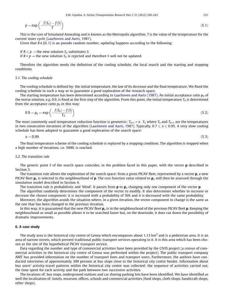
We designed 9 parking lots: 2 internal to the pedestrian area (parking lots n. 10 and 11) and 7 on the pedestrian areaborder (parking lots n. 1, 2, 3, 4, 5, 6, 7). We have defined for each parking lot an influence area with a circular shape and300 m radius. Within each area we have identified the type and the number of attractors that require more a stop of 1 h.We considered the following attractors: museums, art galleries and exhibitions, schools, offices and hotels. In Fig. 2 the influ-ence areas of each parking lot is shown as well as the localisation of the attractors. A weight has been assessed for eachattractor: for museums, art galleries and exhibitions, the weight is proportional to the annual number of visits; for schools,the weight is proportional to the number of students; for offices, the weight is proportional to the number of employees andfor hotels it is proportional to the number of rooms. The attractivity of each parking lot is a function of the number of attrac-tors within its influence area and their relative weights.

The streets within the historical city centre were divided in 50 m long sections and 120 sections resulted. Each section isrepresented by a node and each node is characterised by an attractivity. In each section we identified the number of com-mercial activities and their category (food shops, cloth shops, handicraft shops, other shops). A weight has been assessed foreach category according with the data collected in the field: the weight is proportional to the number of times the category ofcommercial activities has been visited by the interviewees in their trip chains. The attractivity of each node is a function ofthe number and weights of commercial activities within the section.

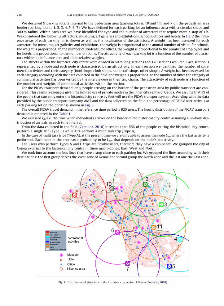
For the PICAV transport demand, only people arriving on the border of the pedestrian area by public transport are con-sidered. This seems reasonable given the limited use of private modes in the inner city centre of Genoa. We assume that 1% ofthe people that currently enter the historical city centre by foot will use the PICAV transport system. According with the dataprovided by the public transport company AMT and the data collected on the field, the percentage of PICAV user arrivals ateach parking lot on the border is shown in Fig. 3.

The overall PICAV travel demand in the reference time period is 925 users. The hourly distribution of the PICAV transportdemand is reported in the Table 1.

We assessed ti0, i.e. the time when individual i arrives on the border of the historical city centre assuming a uniform dis-tribution of arrivals in each time interval.

From the data collected in the field (Cepolina, 2010) it results that: 55% of the people exiting the historical city centre,perform a single trip (Type B) while 45% perform a multi task trip (Type A).

In the case of multi task trips (Type A), at the present time we are only able to assess the node Lina where the last activity isperformed. Each node in the area has a probability to be Lina, that depends on the node’s attactivity.

The users who perform Types A and C trips are flexible users, therefore they have a choice set. We grouped the city ofGenoa external to the historical city centre in three macro-zones: East, West and North.

We took into account the bus lines that have a stop close to each parking lot. We grouped the lines according with theirdestinations: the first group serves the West zone of Genoa, the second group the North zone and the last one the East zone.

Fig. 2. Distribution of attractors in the historical city centre of Genoa (Bonfanti, 2010).

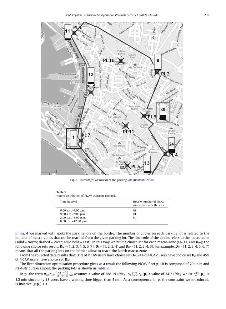
Fig. 3. Percentages of arrivals at the parking lots (Bonfanti, 2010).

Table 1Hourly distribution of PICAV transport demand.

Time interval Hourly number of PICAVusers that enter the area

6:00 a.m.–9:00 a.m. 689:00 a.m.–2:00 p.m. 612:00 p.m.–8:00 p.m. 648:00 p.m.–12:00 p.m. 8


In Fig. 4 we marked with spots the parking lots on the border. The number of circles on each parking lot is related to thenumber of macro-zones that can be reached from the given parking lot. The line code of the circles refers to the macro-zone(solid = North; dashed = West; solid bold = East). In this way we built a choice set for each macro-zone (DN, DE and DW); thefollowing choice sets result: DN = (1, 2, 3, 4, 5, 6, 7); DE = (1, 2, 3, 4) and DW = (1, 2, 3, 4, 6). For example, DN = (1, 2, 3, 4, 5, 6, 7)means that all the parking lots on the border allow to reach the North macro-zone.

From the collected data results that: 31% of PICAV users have choice set DN; 24% of PICAV users have choice set DE and 45%of PICAV users have choice set DW.

The fleet dimension optimisation procedure gives as a result the following PICAV fleet p�: it is composed of 70 units andits distribution among the parking lots is shown in Table 2.

In p� the term nvehcvehrð1þrÞlt

ð1þrÞlt�1

h i1

365 assumes a value of 288.19 €/day; cwPm

i¼1twiðpÞ a value of 34.7 €/day whilst t90%w ðp�Þ is

1.2 min since only 18 users have a waiting time bigger than 5 min. As a consequence, in p� the constraint we introduced,is inactive: g(p�) < 0.

Fig. 4. Disposition of the seven parking lots with reference to the three outer areas of Genoa (Bonfanti, 2010).

Table 2Optimal distribution of PICAV fleet among the nine parking lots.

Parking lotnumber

Number of PICAV units at the parking lot at timet = 0

1 82 93 104 105 116 77 5

10 511 5


To understand better the characteristics of the f(p) function, we assessed its values for five PICAV fleets.All considered cases make reference to a constant distribution of vehicles among the parking lots: the percentage of PICAV

units in each parking lot is the one related to the optimal distribution shown in Table 2. The five PICAV fleets are:

– The optimum fleet dimension, which is equal to 70 vehicles.– A fleet dimension equal to 61 vehicles, i.e. the number of vehicles in each parking lot has been decreased by 1 unit from

the optimum.– A fleet dimension equal to 52 vehicles, i.e. the number of vehicles in each parking lot has been decreased by 2 units.– A fleet dimension equal to 79 vehicles, i.e. the number of vehicles has been increased by 1 unit.– A fleet dimension equal to 88 vehicles, i.e. the number of vehicles lot has been increased by 2 units.

In Fig. 5, the value of the function and the values of its two component terms are shown against the five fleets. From thefigure it can be seen that the derivatives of the two terms assume the same value (and opposite sign) when the total userwaiting time is very low. It has to be noted that the function values do not have any meaning since the function does nottake into account flat costs.

Other researchers studied the performance of shared vehicle systems. In particular Barth and Todd (1999) developed amodel and applied it to a resort community in Southern California. Their model shows that the shared vehicle system is most

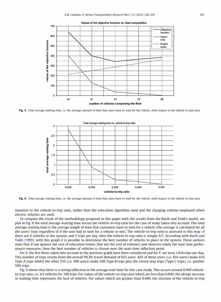
Fig. 5. Total average waiting time, i.e. the average amount of time that users have to wait for the vehicle, with respect to the vehicle to trip ratio.

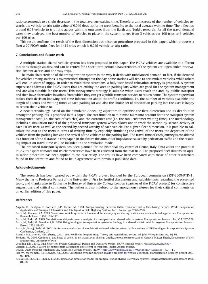
Fig. 6. Total average waiting time, i.e. the average amount of time that users have to wait for the vehicle, with respect to the vehicle to trip ratio.


sensitive to the vehicle-to-trip ratio, rather than the relocation algorithm used and the charging scheme employed whenelectric vehicles are used.

To compare the result of the methodology proposed in this paper with the results from the Barth and Todd’s model, weplot in Fig. 6 the total average waiting time versus the vehicle-to-trip ratio for the case of study taken into account. The totalaverage waiting time is the average length of time that customers have to wait for a vehicle (the average is calculated for allthe users’ trips regardless of if the user had to wait for a vehicle or not). The vehicle-to-trip ratio is assessed in this way: ifthere are X vehicles in the system, and Y trips per day, then the vehicle to trip ratio is simply X/Y. According with Barth andTodd (1999), with this graph it is possible to determine the best number of vehicles to place in the system. These authorsstate that if one ignores the cost of relocation events (but not the cost of vehicles) and observes solely the wait time perfor-mance measures, then the best number of vehicles is chosen near the wait-time inflection point.

For X, the five fleets taken into account in the previous graph have been considered and for Y, we have 1434 trips per day.This number of trips results from the overall PICAV travel demand of 925 users. 45% of these users (i.e. 416 users) make 416Type A trips whilst the other 55% (i.e. 509 users) make 509 Type B trips plus the return way trips (Type C trips), i.e. another509 trips.

Fig. 6 shows that there is a strong inflection in the average wait time for this case study. This occurs around 0.049 vehicle-to-trip ratio, i.e. 4.9 vehicles for 100 trips. For values of the vehicle-to-trip ratio which are less than 0.049, the abrupt increasein waiting time represents the lack of vehicles. For values which are greater than 0.049, the increase of the vehicle-to-trip


ratio corresponds to a slight decrease in the total average waiting time. Therefore, an increase of the number of vehicles to-wards the vehicle-to-trip ratio value of 0.049 does not bring great benefits to the total average waiting time. The inflectionaround 0.05 vehicle-to-trip ratio agrees with the outcomes from the Barth and Todd’s research: for all the travel demandcases they analysed, the best number of vehicles to place in the system ranges from 3 vehicles per 100 trips to 6 vehiclesper 100 trips.

This result confirms the result of the fleet dimension optimisation procedure proposed in this paper, which proposes afleet a 70 PICAV units fleet for 1434 trips which is 0.049 vehicle-to-trip ratio.

7. Conclusions and future work

A multiple station shared vehicle system has been proposed in this paper. The PICAV vehicles are available at differentlocations through an area and can be rented for a short term period. Characteristics of the system are: open ended reserva-tion, instant access and one-way trips.

The main characteristic of the transportation system is the way it deals with unbalanced demand. In fact, if the demandfor vehicles among stations is asymmetrical throughout the day, some stations will tend to accumulate vehicles, while otherswill end up short of supply. In order to avoid these situations, a fully user-based relocation strategy is proposed. A systemsupervisor addresses the PICAV users that are exiting the area to parking lots which are good for the system managementand are also suitable for the users. This management strategy is suitable when users reach the area by public transportand then have alternative locations from which they can get a public transport service to return home. The system supervisormakes their decision knowing real time information about the traffic conditions, i.e. the number of vehicles available, thelength of queues and waiting times at each parking lot and also the choice set of destination parking lots the user is happyto return their vehicle to.

A new methodology, based on the Simulated Annealing algorithm to optimise the fleet dimension and its distributionamong the parking lots is proposed in this paper. The cost function to minimise takes into account both the transport systemmanagement cost (i.e. the cost of vehicles) and the customer cost (i.e. the total customer waiting time). The methodologyincludes a simulation model of the proposed transport system which allows one to track the second-by-second activity ofeach PICAV user, as well as the second-by-second activity of each vehicle. For a given fleet dimension, it is possible to cal-culate the cost to the users in terms of waiting time by explicitly simulating the arrival of the users, the departure of thevehicles from the parking lots and the arrival of the vehicles to the parking lots. The travel time of each journey is consideredas a function of the distance in this paper. In the future the amount of impedance caused by pedestrian traffic and the result-ing impact on travel time will be included in the simulation model.

The proposed transport system has been planned for the historical city centre of Genoa, Italy. Data about the potentialPICAV transport demand and its characteristics have been collected from the real field. The proposed fleet dimension opti-misation procedure has been applied to the case study. The results have been compared with those of other researchersfound in the literature and found to be in agreement with previous published data.

Acknowledgements

The research has been carried out within the PICAV project founded by the European commission (SST-2008-RTD-1).Many thanks to Professor Ferrari of the University of Pisa for fruitful discussions and valuable hints regarding the presentedtopic, and thanks also to Catherine Holloway of University College London (partner of the PICAV project) for constructivesuggestions and critical comments. The author is also indebted to the anonymous referees for their critical comments onan earlier edition of this paper.

References

Augello, D., Benéjam, E., Nerrière, J.-P., Parent, M., 1994. Complementary between Public Transport and a Car-Sharing Service. World Congress onApplications of Transport Telematics and Intelligent Vehicle Highway System, Paris, France, pp. 2985–2992.

Barth, M., Shaheen, S.A., 2003. Shared-use vehicle systems: a framework for classifying carsharing, station cars, and combined approaches. TransportationResearch Record 1791, 105–112.

Barth, M., Todd, M., 1999. Simulation model performance analysis of a multiple station shared vehicle system. Transportation Research Part C 7, 237–259.Barth, M., Todd, M., Murakami, H., 2000. Using intelligent transportation system technology in a shared electric vehicle program. Transportation Research

Record 1731, 88–95.Barth, M., Han, J., Todd, M., 2001. Performance evaluation of a multistation shared vehicle system. In: Proceedings of IEEE Intelligent Transportation Systems

Conference, Oakland, US.Bazaraa, M.S., Sherali, H.D., Shetty, C.M., 1993. Nonlinear Programming: Theory and Algorithms, second ed. John Wiley & Sons Inc., NJ, US.Bonfanti, M., 2010. Gestione di una flotta di veicoli di un sistema car-sharing: applicazione al centro urbano di Genova. Master Thesis, Department of Civil

Engineering, University of Pisa.Cepolina, E.M., 2010. D2.2 Report on System Conceptual Design and Operative Modes. PICAV Internal Report. <http://www.picav.eu>.Cherchi, E., 2003. Il valore del tempo nella valutazione dei sistemi di trasporto. Franco Angeli, Milano.DIMEC, 2009. Personal Intelligent City Accessible Vehicle System. PICAV. <http://www.dimec.unige.it/PMAR/picav/> (accessed 17.01.11).Fan, W., Machemehl, R.B., Lownes, N.E., 2008. Carsharing dynamic decision-making problem for vehicle allocation. Transportation Research Record 2063,

97–104.Kek, A.G.H., Cheu, R.L., Chor, M.L., 2006. Relocation simulation model for multiple-station shared-use vehicle systems. Transportation Research Record 1986,

81–88.

http://www.picav.eu

http://www.dimec.unige.it/PMAR/picav/


Kek, A.G.H., Cheu, R.L., Fung, C.H., 2009. A decision support system for vehicle relocation operations in carsharing systems. Transportation Research Part E 45(1), 149–158.

Laarhoven, J.M., Aarts, E.H.L., 1987. Simulated Annealing: Theory and Applications. Kluver Academic Publishers, Dordrecht, NL.Mukai, N., Watanabe, T., 2005. Dynamic location management for on-demand car sharing system. In: Howlett, R.J., Jain, L.C., Khosla, R. (Eds.), Knowledge-

Based Intelligent Information and Engineering Systems, vol. 3681. Springer-Verlag GmbH, Berlin Heidelberg, pp. 768–774.Shaheen, S.A., Cohen, A.P., 2007. Growth in worldwide carsharing – an international comparison. Transportation Research Record 1992, 81–89.Shaheen, S.A., Cohen, A.P., Roberts, J.D., 2006. Carsharing in North America – market growth, current developments, and future potential. Transportation

Research Record 1986, 116–124.Van Rossum, G., 2006. Python Tutorial. Release 2.5. <http://docs.python.org/release/2.5/tut/tut.html> (accessed 17.01.11).

http://docs.python.org/release/2.5/tut/tut.html