


Bahasa
Halaman
Hukum

Research Article
A multiway approach for classification andcharacterization of rabbit liver apothioneinsby CE-ESI-MS
We applied a multiway approach to extract information from the analysis of protein
isoforms by CE-ESI-MS. Metallothioneins (MT) are low-molecular-weight proteins
(6–7 kDa) with a strong affinity for heavy-metal ions. Rabbit liver MT-I and MT-II
fractions are purified from MT samples. At low pH, the bound metal ions were released
from the amino acid structures, giving rise to apothioneins. MT-I, MT-II and MT
apothioneins, which are complex mixtures of protein isoforms, were analyzed by CE-ESI-
MS. After data pre-processing, parallel factor analysis (PARAFAC) and multivariate curve
resolution-alternating least squares (MCR-ALS) were applied to the data sets. In both
cases, the models enabled classification of the protein samples and identification of their
characteristic sub-isoforms using a set of three components. MCR-ALS required an
initial estimate of the pure mass spectra of the three components. Thus, PARAFAC
loadings were used to initialize the MCR-ALS optimization. The classifications obtained
with MCR-ALS were slightly better than those obtained with PARAFAC, probably
because MCR-ALS was less affected by the small migration time shifts of the pre-
processed electropherograms. However, no differences were found between the pure
mass spectra of the three components in either model. Finally, MCR-ALS allowed us to
obtain an individual electrophoretic profile of each of the three components for each of
the samples analyzed, which proved valuable for characterization and quantification
purposes.
Keywords:
CE-MS / Isoforms / MCR-ALS / Metallothioneins / PARAFACDOI 10.1002/elps.200800212
1 Introduction
CE is one of the techniques of choice for separation of the
protein isoforms that are a result of microheterogeneity
arising in the biosynthesis of a large number of proteins
[1–4]. In CE, protein isoforms (e.g. apothioneins of metallo-
forms, metalloforms or glycoforms) are primarily separated
according to their charge-to-mass ratios, and despite its
limited selectivity, UV absorbance detection is used
extensively for detection [5–7]. In recent years, CE coupled
online with ICP-MS has proved to be useful for quantitative
speciation of several metals in metalloproteins [8]. However,
CE-ICP-MS is unsuitable for obtaining molecular mass
(Mm) information from the different apothionein metallo-
forms. For this purpose, CE-ESI-MS is preferred [1–4, 6–7,
9]. Several CE-ESI-MS have been described for the selective
separation and characterization of protein isoforms [1–4,
6–7, 9]. However, the performance of CE-ESI-MS is limited
and resolution problems could arise when handling
complex mixtures of protein isoforms, such as human
erythropoietin, which is a mixture of around 100 glycoforms
[9]. In such cases, the methods traditionally used for the
analysis of MS data may be excessively time consuming.
Chemometrics-assisted multiway data analysis is an
excellent alternative for handling these complex data sets
[10–14].
Multiway data analysis methods in combination with
CE-UV have been used for sample classification and char-
acterization, peak purity analysis, peak resolution and
quantification [10]. In general, UV absorbance at a single
wavelength as a function of migration time (first-order data
for a single sample or two-way data for a set of samples) or
UV spectra, acquired with a DAD, as a function of migration
time (second-order data for a single sample or three-way
data for a set of samples) have been employed for the
Fernando Benavente1
Balbina Andon1
Estela Gimenez1
Alejandro C. Olivieri2
Jose Barbosa1
Victoria Sanz-Nebot1
1Departamento de QuımicaAnalıtica, Universidad deBarcelona, Barcelona, Espana
2Departamento de QuımicaAnalıtica, Facultad de CienciasBioquımicas y Farmaceuticas,Universidad Nacional deRosario, Rosario, Argentina
Received March 31, 2008Revised June 19, 2008Accepted June 20, 2008
Abbreviations: ALS, alternating least squares; MCR,
multivariate curve resolution; Mm, molecular mass; MT,
metallothioneins; PARAFAC, parallel factor analysis; TIE,
total iron electropherogram
Correspondence: Dr. Fernando Benavente, Departamento deQuımica Analıtica, Universidad de Barcelona, Diagonal 647,E-08028 Barcelona, EspanaE-mail: [email protected]: 134-934021233
& 2008 WILEY-VCH Verlag GmbH & Co. KGaA, Weinheim www.electrophoresis-journal.com
Electrophoresis 2008, 29, 4355–4367 4355
analysis of low-molecular-weight pharmaceuticals, biologi-
cal samples and foodstuffs [10]. Using three-way data,
determinations in the presence of unknown interferences
are possible, when the instrumental signals are separated
mathematically by achieving the second-order advantage [11].
We have recently demonstrated that a first-order multivariate
calibration method with partial least squares (PLS) can be
used to characterize mixtures of different erythropoietin
samples based on the analysis of the electrophoretic separa-
tions of their glycoforms at a single wavelength [12].
However, the use of second-order CE-DAD data for multiway
analysis of individual protein isoforms is precluded because
the UV spectra of the comigrating isoforms are indis-
tinguishable from each other. In order to circumvent this
problem, a detector with enhanced selectivity, such as a mass
spectrometer [1–4], is necessary. To date, a few multiway data
analysis methodologies have been described using CE-ESI-
MS data [13, 14], but to the best of our knowledge, none is
related to the analysis of protein isoforms.
Metallothioneins (MT) form a large family of low-
molecular-weight proteins (6–7 kDa) primarily present in
almost all life forms. MT bind heavy metal ions like
cadmium, zinc or copper, because of their significant
cysteine content [15, 16]. As a result, these proteins contri-
bute to many biological processes involving metal ions [17].
Dysfunctions in MT metabolism have been related to
Alzheimer’s and Wilson’s diseases, several cancers and
immunological disorders [18, 19]. For these reasons, MT
have been postulated as biomarkers of metal pollution or
possible diagnostic tools [18–20].
In addition to polymorphism due to its variable metallic
content, an MT of a particular species exists as a mixture of
several isoforms with slight differences in their amino acid
sequences. Historically, MT have been classified into two
main groups of isoforms on the basis of their elution order
by anionic-exchange chromatography: MT-I and MT-II
[17, 21]. In mammals, this conventional classification based
on charge differences currently coexists with another based
on the absence (MT-1) or presence (MT-2) of an acidic
amino acid residue (Asp (D)) at position 11 or 12 of the
sequence [21]. MT-1 and MT-2 are the isoforms most widely
expressed in tissues and they have received the most
attention. Isoforms with minor differences, such as one
amino acid residue, are classified as subgroups of these two
major isoforms and termed sub-isoforms. The sub-isoforms
are designated by a lower-case letter, e.g. MT-1a. At low pH,
the bound metal ions of MT sub-isoforms are released from
the amino acid structures, giving rise to apothionein sub-
isoforms. High-performance separations coupled to high-
resolution characterization techniques are key tools for
clarifying the specific biological role of metallated and apo
sub-isoforms, which is still unknown [1–4, 8]. Furthermore,
exploring multiway data analysis models for the study
of the relatively simple CE-ESI-MS data sets obtained
for the analysis of different MT samples constitutes an
excellent benchmark for the study of proteins with a greater
microheterogeneity.
In this paper, parallel factor analysis (PARAFAC)
[22–24] and multivariate curve resolution- alternating least-
squares (MCR-ALS) [25, 26] are applied to the development
of second-order multiway data analysis methods for inves-
tigation of different samples of rabbit liver apothioneins.
Several data pre-processing steps are proposed before model
optimization. The performance of the two models is then
compared and major advantages and disadvantages are
discussed in detail. In general, the results confirm that both
PARAFAC and MCR-ALS give a rapid and simple classifi-
cation of the protein samples and identification of their
characteristic sub-isoforms.
2 Materials and methods
2.1 Chemicals and reagents
All chemicals were of analytical reagent grade and used as
received. Acetic acid (glacial) and formic acid (98–100%) for
the separation electrolytes were purchased from Merck
(Darmstadt, Germany). Trifluoroacetic acid employed for
sample pre-treatment and 2-propanol for sheath liquid
preparation were also supplied by Merck. Water with a
specific conductivity lower than 0.05 ms/cm was obtained
by using a Milli-Q water purification system (Millipore,
Molsheim, France).
Rabbit liver MT (batch no. 20K7000, 4.7% Cd and 0.5%
Zn), MT-I (batch no. 80K7012, 8.0% Cd and 1.2% Zn) and
MT-II (batch no. 20K70130, 7.9% Cd and 1.4% Zn) were
obtained from Sigma-Aldrich (St. Louis, MO, USA). The
manufacturer reported that MT-I and MT-II were obtained
from MT samples by means of a double-step procedure.
After purification of a rabbit liver extract by size exclusion
chromatography, the isolated MT-containing fraction was
subjected to anion-exchange chromatography at neutral pH,
obtaining MT-I and MT-II fractions that contained sub-
isoforms that differed by a single global charge. Stock
solutions of MT were prepared by dissolving 1 mg of protein
in 1 mL of water. They were stored at�181C in the dark
when not in use.
2.2 CE-ESI-MS
All CE-ESI-MS experiments were performed using an
Agilent Technologies HP3DCE system (Waldbronn,
Germany) coupled to an MSD Ion Trap mass spectrometer
with a G1603A sheath-flow CE-ESI-MS interface (Agilent
Technologies) [6]. The sheath liquid was delivered by an
infusion pump KD Scientific 100 Series (Holliston, MA,
USA) at a flow rate of 3.3 mL/min. A 100 cm LT� 75 mm id
bare fused-silica capillary supplied by Polymicro Technolo-
gies (Phoenix, AZ, USA) was used for the electrophoretic
separations. The parameters of the mass spectrometer were
automatically tuned by direct infusion of a 1 mg/L solution
of the MT-II sample. The sample solution was infused at
Electrophoresis 2008, 29, 4355–43674356 F. Benavente et al.
& 2008 WILEY-VCH Verlag GmbH & Co. KGaA, Weinheim www.electrophoresis-journal.com
50 mbar through the separation capillary, while the signal
for one of the multiply charged molecular ions of the
predominant MT-2a sub-isoform ([MT-2a+5H]5+ 5 1226.1
m/z, see Table 1) was maximized. Full scan mass spectra
were acquired in the m/z range from 500 to 2200 m/z at
intervals of 0.1 m/z (as an average of every seven scans). All
experiments were done in positive mode and the ESI voltage
and the end plate offset were set at 4100 and �500 V,
respectively. Voltages on capillary exit and skimmer were
240 and 42 V, respectively. Octopole voltages were set at 24
and 1 V and octopole radiofrequency at 128 Vpp. Lens were
�7 and �67 V and trap drive 133 (arbitrary units). Nebulizer
gas (N2) pressure was 7 p.s.i., drying gas (N2) flow rate was
2 L/min and drying temperature was set at 3001C. Instru-
ment control, data acquisition and data processing were
performed using the CE/MSD Trap Software 6.1 (Agilent
Technologies).
pH was measured with a Crison 2002 potentiometer
(Crison Instruments, Barcelona, Spain), equipped with a
ROSS electrode 8102 (Orion Research, Boston, MA, USA).
2.3 Experimental procedures
2.3.1 Sample pre-treatment
Cadmium and zinc from rabbit liver MT were eliminated
before CE-ESI-MS analysis; 100 mL of 1 mg/mL solutions of
MT, MT-I and MT-II samples were acidified with TFA (final
concentration was 0.1% v/v). The acidic samples were
desalted by size exclusion filtration through MicroSpin
G-25 microcolumns containing a SephadexTM sorbent
(Amersham Biosciences, Uppsala, Sweden), following the
manufacturer’s instructions. Apothionein samples resulting
from this treatment were injected immediately after their
preparation to avoid oxidation. For ease of understanding,
apothionein isoforms and sub-isoforms are abbreviated as
MT throughout the text.
All samples were passed through a 0.45 mm nylon filter
(MSI, Westboro, MA, USA) before analysis and were stored
at 41C when not in use.
2.3.2 CE-ESI-MS
The CE-ESI-MS method was developed in an earlier study
using a TOF-MS detector [6]. The separation electrolyte
contained 50 mM of acetic acid and 50 mM of formic acid
(pH 2.3) and was passed through a nylon filter of 0.45 mm
(MSI) before analysis. A sheath liquid of 50:50 v/v
2-propanol:water with 1% v/v of acetic acid resulted in
optimum detection sensitivity. It was degassed for 10 min by
sonication before use. All capillary rinses were performed at
930 mbar. New capillaries were flushed for 20 min with
aqueous 1 M NaOH, followed by 15 min with water and
30 min with separation electrolyte solution. The system was
finally equilibrated by applying the separation voltage for
15 min. The activation procedure was performed off-line
and ESI voltage was switched off in order to avoid the
unnecessary entrance of NaOH into the MS system.
Samples were hydrodynamically injected at 30 mbar for
5 s. Analyses were carried out at 251C under normal polarity.
A separation voltage of 25 kV was employed for the
electrophoretic separations, while the ESI voltage was
applied at the MS entrance. MT-I , MT-II and MT samples
were analyzed on four different days using a new separation
capillary each day, resulting in 10, 10 and 3+3 electro-
phoretic runs each day, respectively. Between runs, the
capillary was rinsed for 3 min with separation buffer.
Capillaries were discarded after each working day. The
separation electrolyte and the sheath liquid were stored at
41C when not in use.
2.4 Data analysis
2.4.1 Software
Matlabs for Windows (version 7.0) was used for data pre-
processing, programming, calculations and graphical repre-
sentation, unless otherwise indicated. MassLynx (version
3.5) was the software supplied with the mass spectrometers
of Micromass (Manchester, UK) for control, data acquisition
and data processing. DataBridge was a file converter
provided with Masslynx. ESI mass spectra were deconvo-
luted using MaxEnt1 (Micromass), which uses an algorithm
based on the method of maximum entropy to find the
simplest zero charge Mm spectrum that could account for
the observed m/z data. EDit was a free C++ program for
conversion of MassLynx continuum spectra into a matrix
format suitable for direct introduction into scientific
graphing packages [27]. A laboratory-written Matlab routine
was employed for the rest of the data-pre-processing. This
routine needed Moving_average2 for smoothing, which
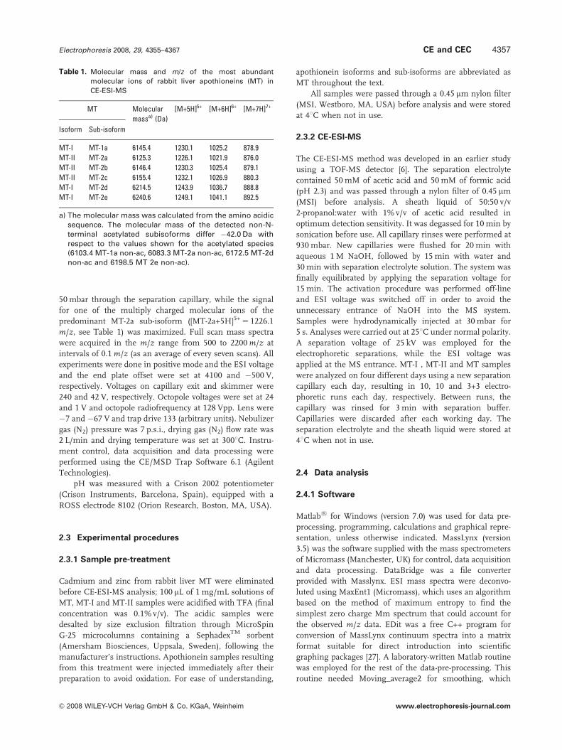
Table 1. Molecular mass and m/z of the most abundant
molecular ions of rabbit liver apothioneins (MT) in
CE-ESI-MS
MT Molecular
massa) (Da)
[M+5H]5+ [M+6H]6+ [M+7H]7+
Isoform Sub-isoform
MT-I MT-1a 6145.4 1230.1 1025.2 878.9
MT-II MT-2a 6125.3 1226.1 1021.9 876.0
MT-II MT-2b 6146.4 1230.3 1025.4 879.1
MT-II MT-2c 6155.4 1232.1 1026.9 880.3
MT-I MT-2d 6214.5 1243.9 1036.7 888.8
MT-I MT-2e 6240.6 1249.1 1041.1 892.5
a) The molecular mass was calculated from the amino acidicsequence. The molecular mass of the detected non-N-terminal acetylated subisoforms differ �42.0 Da withrespect to the values shown for the acetylated species(6103.4 MT-1a non-ac, 6083.3 MT-2a non-ac, 6172.5 MT-2dnon-ac and 6198.5 MT 2e non-ac).
Electrophoresis 2008, 29, 4355–4367 CE and CEC 4357
& 2008 WILEY-VCH Verlag GmbH & Co. KGaA, Weinheim www.electrophoresis-journal.com

was available through the file exchange service of the
MATLAB website [28]. The routine for PARAFAC was freely
available on the internet as part of an N-way Toolboxfor MATLAB [29]. A graphical user-friendly interface for
MCR-ALS was also freely available online on the authors’
website [30].
2.4.2 Data pre-processing
Recovery of data from the CE-ESI-MS electropherograms of
each sample in an appropriate text format was a trouble-
some procedure. When the CE-ESI-MS raw files were
directly converted into ASCII format by use of the CE/MSD
Trap Software 6.1 provided with the instrument, the
resulting files were useless for further data analysis. As an
alternative, we found it necessary to first convert these raw
files into continuum NetCDF format by use of the CE/MSD
Trap Software 6.1. Then the NetCDF files were converted
into the MassLynx environment employing the DataBridge
program, prior to finally turning the continuum Masslynx
files into ASCII format, again using DataBridge. Following
this procedure, each of the generated text files consisted of a
sequence over time of the acquired spectra listed as m/zversus intensity [27]. EDit was employed to convert the ASCII
files obtained with Masslynx into a matrix in comma
separated value format, which was readable by numerical
computing programs such as Matlab. A matrix obtained
with EDit consisted of a single data matrix, the columns of
which contained the mass spectra at the different migration
times, while the rows contained the electrophoretic profiles
at the different m/z values. The first column and the first
row did not contain intensity values, but rather the m/zvalues and the time values, respectively. The dimensions of
the EDit matrix could be specified before the conversion in
order to resize the original raw data. In our case, a
preliminary inspection of the raw CE-ESI-MS electropher-
ograms with the CE/MSD Trap Software 6.1 was helpful for
reducing both the m/z and the time dimensions of the data
matrix. An m/z range between 600.1 and 1499.9 (at intervals
of 0.1 m/z) was selected for all the electropherograms
according to the m/z values of the [M+5H]5+, [M+6H]6+and
[M+7H]7+ molecular ions of the MT-I, MT-II and MT sub-
isoforms, which were the most abundant molecular ions in
their mass spectra [6] (see Table 1). In contrast, a different
time window was selected for each electropherogram, but
always centered on the region where the electrophoretic
peaks were appearing, and with the precaution of selecting
the same number of migration times, i.e. columns. In this
way, 8999� 240 data matrices were obtained after
being processed with EDit. The first column was immedi-
ately eliminated because it contained the same m/z values in
all cases.
Each 8999� 239 matrix obtained as indicated above was
processed by the following procedure. The mass spectra of
the first 20 columns, where no electrophoretic peaks were
detected, were averaged in order to obtain a background
mass spectrum. The background mass spectrum was
subtracted from the mass spectra of each column. Then, the
first 20 columns of the matrix were discarded. The intensity
values of the background-subtracted 8999� 219 matrix were
smoothed by a moving average function (X, M, N), which
smoothed the matrix X by averaging each element with the
surrounding elements that fit in a box of (2M+1)� (2N+1)
centered on that element (M and N were both 1). In order to
correct for the variability in the migration times, once the
intensity values of the matrix were smoothed, the migration
timescale of the first row was converted into a migration
time ratio (t/tr) scale [31]. As MT-1a and MT-2b sub-isoforms
had the same electrophoretic mobility at the separation pH
value [6], in all cases it was employed as a time reference (tr),
the time corresponding to the maximum intensity at
an m/z value of 1230.1 (70.4), which corresponded to the
[MT-1a+5H]5+ molecular ion in MT-I and MT samples and
to the [MT-2b+5H]5+ molecular ion in MT-II and MT
samples (Table 1). All the intensity values were normalized
to the maximum intensity found in the matrix. The final
data set for multivariate data analysis consisted of 25 pre-
processed matrices (8999� 219), 10 for the MT-I, 10 for the
MT-II and 6 for the MT sample. The pre-processed matrices
could be represented as a total ion electropherogram (TIE)
where the intensities in each row were summed over all the
m/z values.
2.4.3 Multiway data analysis
Both PARAFAC [22–24, 29, 32, 33] and MCR-ALS [25, 26,
30, 34, 35] models have been discussed in detail elsewhere
and only a brief description is presented here. Before data
analysis, the first row from the pre-processed matrices,
which contained the t/tr scale, was eliminated, the
minimum value of intensity was summed to all the matrix
elements in order to avoid negative values and the resulting
matrix transposed. Each J�K DI matrix (I 5 25) consisted of
a two-way array with J times and K m/z ratios (J 5 219 and
K 5 8998). When all DI matrices were stacked one on top of
another, a three-way data array Dpar with dimensions
I� J�K, was obtained for processing with PARAFAC.
Alternatively, for MCR-ALS analysis, a column-wise
augmented data matrix (Daug) was created, with dimensions
(IJ)�K.
Neither PARAFAC nor MCR-ALS routines could be run
on our PC (Intel Core 2 Duo E6600 at 2.4 GHz with 4 GB
RAM) using 219� 8998 DI matrices after building Dpar or
Daug. Thus, two sets of reduced DI matrices were
generated. A set of 219� 3000 DI matrices was obtained
after taking into account one of every three m/z values of
the original 219� 8998 DI matrix for each row. In
addition, a set of 219� 1286 DI matrices was generated
after considering one of every seven m/z values. PARAFAC
could be run employing both reduced DI sets. For MCR-ALS
it was necessary to build Daug from the 219� 1286 DI
matrices.
Electrophoresis 2008, 29, 4355–43674358 F. Benavente et al.
& 2008 WILEY-VCH Verlag GmbH & Co. KGaA, Weinheim www.electrophoresis-journal.com
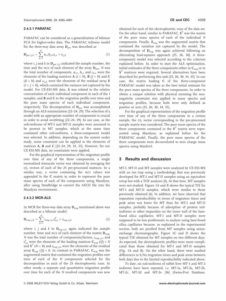
2.4.3.1 PARAFAC
PARAFAC can be considered as a generalization of bilinear
PCA for higher-order data. The PARAFAC trilinear model
for the three-way data array Dpar was described as
Dpar i;j;k ¼XN
n¼1
ai;nbj;nck;n þ ei;j;k ð1Þ
where i, j and k in Dpar i;j;k indicated the sample number, the
time and the m/z of each element of the array Dpar, N was
the total number of components, ai;n, bj;n and ck;n were the
elements of the loading matrices A (I�N), B (J�N) and C(K�N) and ei;j;k were the elements of the residual array E(I� J�K), which contained the variance not captured by the
model. For CE-ESI-MS data, A was related to the relative
concentration of each individual component in each of the Isamples, and B and C to the migration profile over time and
the pure mass spectra of each individual component,
respectively. The decomposition of Dpar was accomplished
through an ALS minimization [22–24, 29]. The selection of a
model with an appropriate number of components is crucial
in order to avoid overfitting [22–24, 29]. In our case, as the
sub-isoforms of MT-I and MT-II samples were assumed to
be present in MT samples, which at the same time
contained other sub-isoforms, a three-component model
was selected. In addition, depending on the system under
study, some constraint can be applied to the elements of
matrices A, B and C [22–24, 29, 32, 33]. However, for our
CE-ESI-MS data, no constraints were applied.
For the graphical representation of the migration profile
over time of any of the three components, a single
normalized timescale vector was obtained by averaging the
t/tr vectors of each of the 25 pre-processed matrices. In a
similar way, a vector containing the m/z values was
appended to the C matrix in order to represent the pure
mass spectra of each of the components using Masslynx,
after using DataBridge to convert the ASCII file into the
Masslynx environment.
2.4.3.2 MCR-ALS
In MCR the three-way data array Daug mentioned above was
described as a bilinear model:
Daug i;j;k ¼XN
n¼1
caug i;j;nsTn;k þ eaug i;j;k ð2Þ
where i, j and k in Daug i;j;k again indicated the sample
number, time and m/z of each element of the matrix Daug,
N was the total number of components/factors, caug i;j;n and
sTn;k were the elements of the loading matrices Caug (IJ)�N
and ST (N�K) and eaug i;j;k were the elements of the residual
array Eaug (IJ)�K. In contrast to PARAFAC, Caug was the
augmented matrix that contained the migration profiles over
time of each of the N components selected for the
decomposition in each of the 25 electrophoretic runs. In
other words, a separate and quantitative migration profile
over time for each of the N resolved components was now
obtained for each of the electrophoretic runs of the data set.
On the other hand, similar to PARAFAC, ST was the matrix
of the pure mass spectra of each of the individual Ncomponents. Finally, Eaug was the augmented matrix that
contained the variation not captured by the model. The
decomposition of Daug was again achieved following an
alternating least-squares approach [25, 26, 30]. A three-
component model was selected according to the criterion
explained before. In order to start the ALS optimization,
initial estimates of the three components either in Caug or in
ST matrices were required. Several alternatives have been
described for performing this task [25, 26, 30, 34, 35]. In our
case, the matrix loading C of the three-component
PARAFAC model was taken as the best initial estimate for
the pure mass spectra of the three components. In order to
obtain a unique solution with physical meaning the non-
negativity constraint was applied to mass spectra and
migration profiles, because both were only defined as
positive or zero [25, 26, 30, 34, 35].
For the graphical representation of the migration profile
over time of any of the three components in a certain
sample, the t/tr vector corresponding to the pre-processed
sample matrix was considered. The pure mass spectra of the
three components contained in the ST matrix were repre-
sented using Masslynx, as explained before for the
PARAFAC model. Finally, the pure mass spectra of the
three components were deconvoluted to zero charge mass
spectra using MaxEnt1.
3 Results and discussion
MT-I, MT-II and MT samples were analyzed by CE-ESI-MS
with an ion trap using a methodology that was previously
developed for MT-I and MT-II samples using an equivalent
setup but with a TOF analyzer [6]. At that time, MT samples
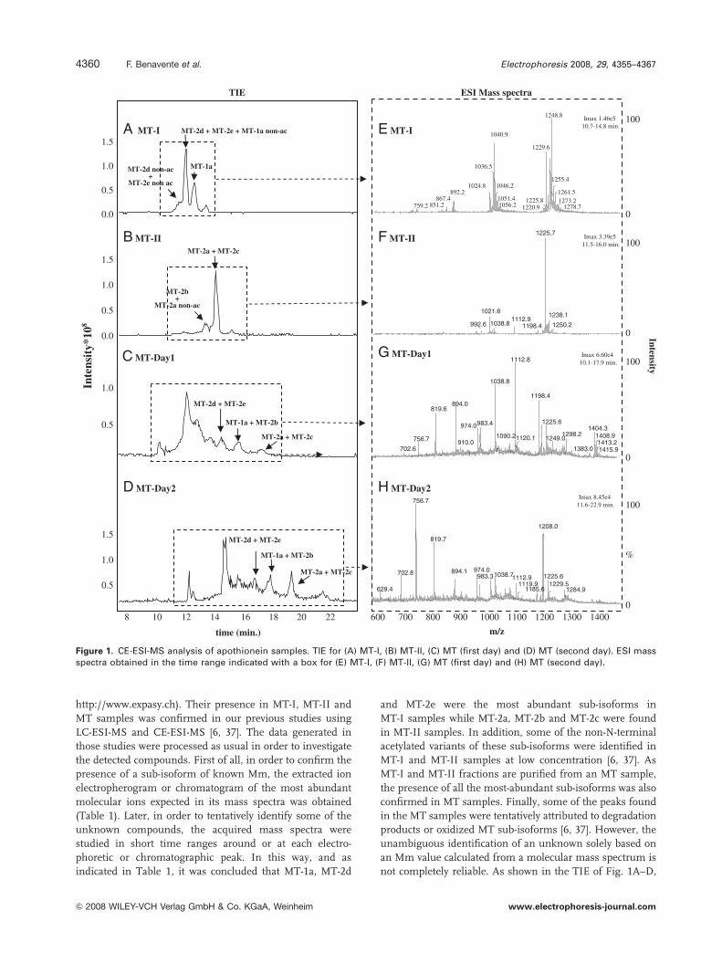
were not studied. Figure 1A and B shows the typical TIE for
MT-I and MT-II samples, which were similar to those
previously obtained [6]. In addition, we have observed that
separation reproducibility in terms of migration times and
peak areas was lower for MT than for MT-I and MT-II
samples, probably because of adsorption of protein sub-
isoforms or other impurities on the inner wall of the bare-
fused silica capillaries. MT-I and MT-II samples were
supposed to be less problematic to analyze using bare-fused
silica capillaries because, as explained in the experimental
section, both are purified from MT samples using anion-
exchange chromatography. Figure 1C and D shows the
typical TIE obtained for MT samples on two different days.
As expected, the electrophoretic profiles were more compli-
cated than those obtained for MT-I and MT-II samples
(Fig. 1A and B). On the other hand, there were marked
differences in S/Ns migration times and peak areas between
both days due to the limited reproducibility indicated above.
To date, six sub-isoforms of rabbit liver MT-1 and MT-2
isoforms have been reported, i.e. MT-1a, MT-2a, MT-2b,
MT-2c, MT-2d and MT-2e [36] (Swiss-Prot Database,
Electrophoresis 2008, 29, 4355–4367 CE and CEC 4359
& 2008 WILEY-VCH Verlag GmbH & Co. KGaA, Weinheim www.electrophoresis-journal.com
http://www.expasy.ch). Their presence in MT-I, MT-II and
MT samples was confirmed in our previous studies using
LC-ESI-MS and CE-ESI-MS [6, 37]. The data generated in
those studies were processed as usual in order to investigate
the detected compounds. First of all, in order to confirm the
presence of a sub-isoform of known Mm, the extracted ion
electropherogram or chromatogram of the most abundant
molecular ions expected in its mass spectra was obtained
(Table 1). Later, in order to tentatively identify some of the
unknown compounds, the acquired mass spectra were
studied in short time ranges around or at each electro-
phoretic or chromatographic peak. In this way, and as
indicated in Table 1, it was concluded that MT-1a, MT-2d
and MT-2e were the most abundant sub-isoforms in
MT-I samples while MT-2a, MT-2b and MT-2c were found
in MT-II samples. In addition, some of the non-N-terminal
acetylated variants of these sub-isoforms were identified in
MT-I and MT-II samples at low concentration [6, 37]. As
MT-I and MT-II fractions are purified from an MT sample,
the presence of all the most-abundant sub-isoforms was also
confirmed in MT samples. Finally, some of the peaks found
in the MT samples were tentatively attributed to degradation
products or oxidized MT sub-isoforms [6, 37]. However, the
unambiguous identification of an unknown solely based on
an Mm value calculated from a molecular mass spectrum is
not completely reliable. As shown in the TIE of Fig. 1A–D,
0.0
0.5
1.0
1.5
8 10 12 14 16 18 20 22
0.0
0.5
1.0
1.5
0.5
1.0
0.5
1.0
1.5
Inte
nsit
y*10
8
A MT-I
B MT-II
C MT-Day1
time (min.)
TIE
D MT-Day2
600 700 800 900 1000 1100 1200 1300 1400
0
100Imax 1.46e5 10.7-14.8 min.
1248.8
1040.9
1036.5
1024.8892.2
867.4759.2 851.2
1229.6
1046.2
1051.4 1225.81056.2 1220.9
1255.4
1261.51273.2
1278.7
E MT-I
ESI Mass spectra
1001225.7
1021.6
992.61112.9
1038.8 1198.4
1238.1
1250.2
Imax 3.39e5 11.5-16.0 min.
0
F MT-II
0
1001112.8
1038.8
894.0819.6
756.7
702.6
974.0
910.0
983.4
1120.11090.2
1198.4
1225.61404.3
1298.21249.0
1383.0
1408.91413.21415.9
Imax 6.60e4 10.1-17.9 min.
m/z
G MT-Day1
Intensity
H MT-Day2
0
100
%
756.7
702.8
629.4
1208.0
819.7
974.0894.1 1038.7983.3 1112.9
1185.61119.9
1225.6
1284.91229.5
Imax 8.45e4 11.6-22.9 min.
MT-2d + MT-2e + MT-1a non-ac
MT-1aMT-2d non-ac+
MT-2e non ac
MT-2a + MT-2c
MT-2b+
MT-2a non-ac
MT-2d + MT-2e
MT-1a + MT-2b
MT-2a + MT-2c
MT-2d + MT-2e
MT-1a + MT-2b
MT-2a + MT-2c
Figure 1. CE-ESI-MS analysis of apothionein samples. TIE for (A) MT-I, (B) MT-II, (C) MT (first day) and (D) MT (second day). ESI massspectra obtained in the time range indicated with a box for (E) MT-I, (F) MT-II, (G) MT (first day) and (H) MT (second day).
Electrophoresis 2008, 29, 4355–43674360 F. Benavente et al.
& 2008 WILEY-VCH Verlag GmbH & Co. KGaA, Weinheim www.electrophoresis-journal.com

the same findings in MT-I, MT-II and MT samples were
observed when the CE-ESI-MS data obtained in this work
were investigated as usual. As in our previous studies [6, 37],
some of the sub-isoforms comigrated and some of the
electrophoretic peaks could not be identified. As an example
of the typical ESI mass spectra for the mixtures of sub-
isoforms found in MT-I, MT-II and MT samples, Fig. 1E–H
shows the mass spectra obtained in the time range indicated
with a box in the TIE of Fig. 1A–D. As shown in Fig. 1E and
F for MT-I and MT-II samples, the m/z values of the
[M+5H]5+, [M+6H]6+ and, in some cases, [M+7H]7+ mole-
cular ions of the most-abundant sub-isoforms can be clearly
observed (compare with Table 1). In contrast, the mass
spectra of MT samples were more complex and noisy
(Fig. 1G and H), being consistent with the above comments
about complexity, sensitivity and reproducibility. It was even
difficult to ensure from visual inspection whether the MT
sample contained, among other compounds, the sub-
isoforms found in MT-I and MT-II samples. Thus, a
multivariate approach could be useful to investigate the
highly complex and overlapping electrophoretic profiles of
MT-I, MT-II and MT samples, which were mainly mixtures
of protein sub-isoforms with multiply-charged mass spectra,
and where peaks occurred that could not be assigned to any
particular compound, but that could also be useful as a
fingerprint for classification.
Before multivariate data analysis, pre-processing of the
raw CE-ESI-MS data was necessary [10, 13, 14, 32–35]. At the
moment, the use of bare-fused silica capillaries and sheath-
flow CE-ESI-MS interfaces are the best alternatives for the
analysis of protein isoforms at acidic pH, because of the
excellent column stability and the acceptable robustness of
the coupling [1–4, 6, 7, 9]. However, in general, the
heterogeneity of CE-ESI-MS data is higher than in LC-ESI-
MS due to the lower reproducibility of migration times and
peak areas [33, 34]. Several more or less sophisticated
methods have been described for peak alignment, time or
signal normalization, noise filtering, and baseline correction
of LC-UV or LC-ESI-MS raw data that could be applied to
CE-UV or CE-ESI-MS [10, 13, 14, 33, 34, 38]. Based on this
idea, the raw CE-ESI-MS electropherograms obtained for the
MT-I, MT-II and MT samples were pre-processed following
a simple strategy for background subtraction, smoothing
and normalization of time and intensity scales. The excel-
lent performance is seen by comparing Fig. 2A with Fig. 2B,
which show the TIE corresponding to the analysis
of the MT-I sample before and after completing data
pre-processing.
PARAFAC and MCR-ALS were selected for the multi-
way data analysis of the pre-processed CE-ESI-MS data
because they are well-known second-order decomposition
methods that have been extensively applied for the analysis
of spectroscopic data [22–26, 29, 30, 32–35]. For modelling,
both required an estimation of the number of compounds
(i.e. components or factors) present. Selection of an appro-
priate number of components can be performed in different
ways and can be a challenging task if no prior information is
available about the studied samples [22–26, 29, 30, 32–35].
In our case, three components were easily selected because,
as discussed before, MT-I, MT-II and MT owned a char-
acteristic CE-ESI-MS fingerprint. Before beginning the
three-component model optimization, the size of the 25 pre-
processed matrices was slightly reduced in order to be able
to run PARAFAC and MCR-ALS routines on our standard
personal computer. MCR-ALS required a slightly higher
amount of RAM memory for model optimization. Thus,
selection of one of every three m/z values from each matrix
row was enough for PARAFAC, while one of every seven
m/z values was necessary for MCR-ALS. However, as no
significant differences were found between results obtained
with PARAFAC using either set of size-reduced matrices,
only the results with PARAFAC and MCR-ALS for the
second size-reduced data set will be discussed.
Figure 3 shows the 3-D scores plot (Fig. 3A), the
resolved electrophoretic profiles of the three components
(Fig. 3B) and their pure mass spectra (Fig. 3C) when the
data were modelled with a three-component PARAFAC
model. The percentage of explained variance was 47.4%.
Inte
nsit
y*10
3
t/tr
8 10 12 14 16 18 200
2
4
6
8
10
12
14
16
Inte
nsit
y*10
7
time (min.)
MT-I raw TIE
MT-I pre-processed TIE
0.6 0.7 0.8 0.9 1 1.1 1.2 1.3 1.4 1.50
1
2
3
4
5
6
7
8
A
B
Figure 2. TIE obtained for MT-I sample (A) before and (B) afterdata pre-processing for background subtraction, smoothing andnormalization of time and intensity scales.
Electrophoresis 2008, 29, 4355–4367 CE and CEC 4361
& 2008 WILEY-VCH Verlag GmbH & Co. KGaA, Weinheim www.electrophoresis-journal.com

In general, the amount of variance explained when analyz-
ing second-order data from complex biological samples or
processes is expected to be lower than the values usually
obtained in the analysis of data from less-troublesome
samples [35]. The low percentage of variance explained by
PARAFAC could be due to the lack of reproducibility in
migration times, which led to lack of trilinearity in the
processed data, one of the conditions required for successful
PARAFAC decomposition. Introducing more than three
components led to a similar fit, because the higher-order
components were likely to fit mostly noise, as they were not
related to another chemical species [22–26, 29, 30, 32–35]. In
the 3-D scores plot of Fig. 3A, each point represents a
particular MT-I, MT-II and MT analysis. As can be observed,
the PARAFAC model allowed very good separation between
the three different protein groups. According to the contri-
bution of each of the three components to the different
groups, the variance of MT-II and MT-I was mainly
explained by the first and the second components, respec-
tively, while all three were necessary for MT. At this point,
600 650 700 750 800 850 900 950 1000 1050 1100 1150 1200 1250 1300 1350 1400 14500
100
0
100
0
100
Imax6.27e31020.8
992.1850.7833.9 973.2
1225.2
1031.3
1190.21041.8
1237.1
1248.3
1040.4
1036.2
1024.3892.0866.8744.3
759.0
1242.7
1228.7
1046.0 1254.6
1267.2
1038.3
893.4819.2
756.2
702.3 824.1
973.2
909.5915.8
983.0
985.1
1112.5
1092.21042.5
1197.9
1116.7
1403.7
1297.31199.3
1228.71241.3
1412.1
Imax5.34e3
I max 3.02e3
i) Score 1
ii) Score 2
iii) Score 3
m/z
Inte
nsit
y
00.1
0.20.3
0.4
0
0.2
0.4
0.6
0.80
0.1
0.2
0.3
0.4
0.5
A B
C
Score 1Score 2
Scor
e 3
MT-I
MT-II
MT_Day 1
MT_Day 2
0.7 0.8 0.9 1 1.1 1.2 1.30
0.05
0.1
0.15
0.2
0.25
0.3
0.35
0.4
0.45
t/tr (average)
Inte
nsit
y
Score 1Score 2
Score 3
Figure 3. Three-component PARAFAC model. (A) 3-D scores plot, (B) resolved electrophoretic profiles of the three components and (C)pure mass spectra of (i) the first, (ii) the second and (iii) the third components.
Electrophoresis 2008, 29, 4355–43674362 F. Benavente et al.
& 2008 WILEY-VCH Verlag GmbH & Co. KGaA, Weinheim www.electrophoresis-journal.com
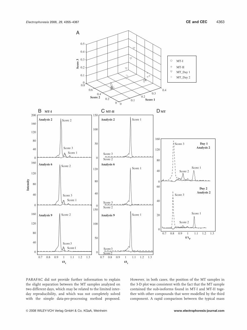
PARAFAC did not provide further information to explain
the slight separation between the MT samples analyzed on
two different days, which may be related to the limited inter-
day reproducibility, and which was not completely solved
with the simple data-pre-processing method proposed.
However, in both cases, the position of the MT samples in
the 3-D plot was consistent with the fact that the MT sample
contained the sub-isoforms found in MT-I and MT-II toge-
ther with other compounds that were modelled by the third
component. A rapid comparison between the typical mass
00.1
0.20.3
0.4
00.2
0.40.6
0.80
0.1
0.2
0.3
0.4
0.5
A
B C D
Score 1Score 2
Scor
e 3 MT-I
MT-II
MT_Day 1
MT_Day 2
MT-I MT-II MT
0
40
80
120
160
200
0
40
80
120
160
0.7 0.8 0.9 1 1.1 1.2 1.3
0
40
80
120
160
t/tr t/tr
Analysis 2
Analysis 6
Analysis 9
Inte
nsit
y
Score 2
Score 3
Score 1
0
50
100
150
0
40
80
120
0.7 0.8 0.9 1 1.1 1.2 1.3
0
50
100
150
Analysis 2
Analysis 6
Analysis 9
Score 1
Score 2
Score 3
0
40
80
120
160
0.7 0.8 0.9 1 1.1 1.2 1.30
20
40
60
t/ tr
Day 1Analysis 2
Day 2Analysis 2
Score 1Score 2
Score 3
Score 2
Score 3
Score 1
Score 2
Score3
Score1
Score 1
Score 2
Score 3
Score 1
Score2
Score3
Score 1
Score 2
Score 3
Electrophoresis 2008, 29, 4355–4367 CE and CEC 4363
& 2008 WILEY-VCH Verlag GmbH & Co. KGaA, Weinheim www.electrophoresis-journal.com
spectra of MT-I, MT-II and MT samples (Fig. 1E–H) and the
pure mass spectra of each of the components retrieved by
PARAFAC (Fig. 3C) confirmed that the first, the second and
the third components were, respectively, related to MT-II,
MT-I and the unknown compounds of the MT samples. As
shown in Fig. 3B, PARAFAC resolved a unique electro-
phoretic profile for each component taking into account
the information from all the analyses. The unknown
compounds of the MT sample migrated first, the sub-
isoforms of the MT-I sample next and the sub-isoforms of
the MT-II last.
In contrast to PARAFAC, MCR-ALS required an initial
estimate of the mass spectra of the three components in
order to start model optimization [25, 26, 30, 34, 35]. In our
case, as the loadings from the three-component PARAFAC
model were available, they were selected as the best initial
estimates for the pure spectra of each of the three compo-
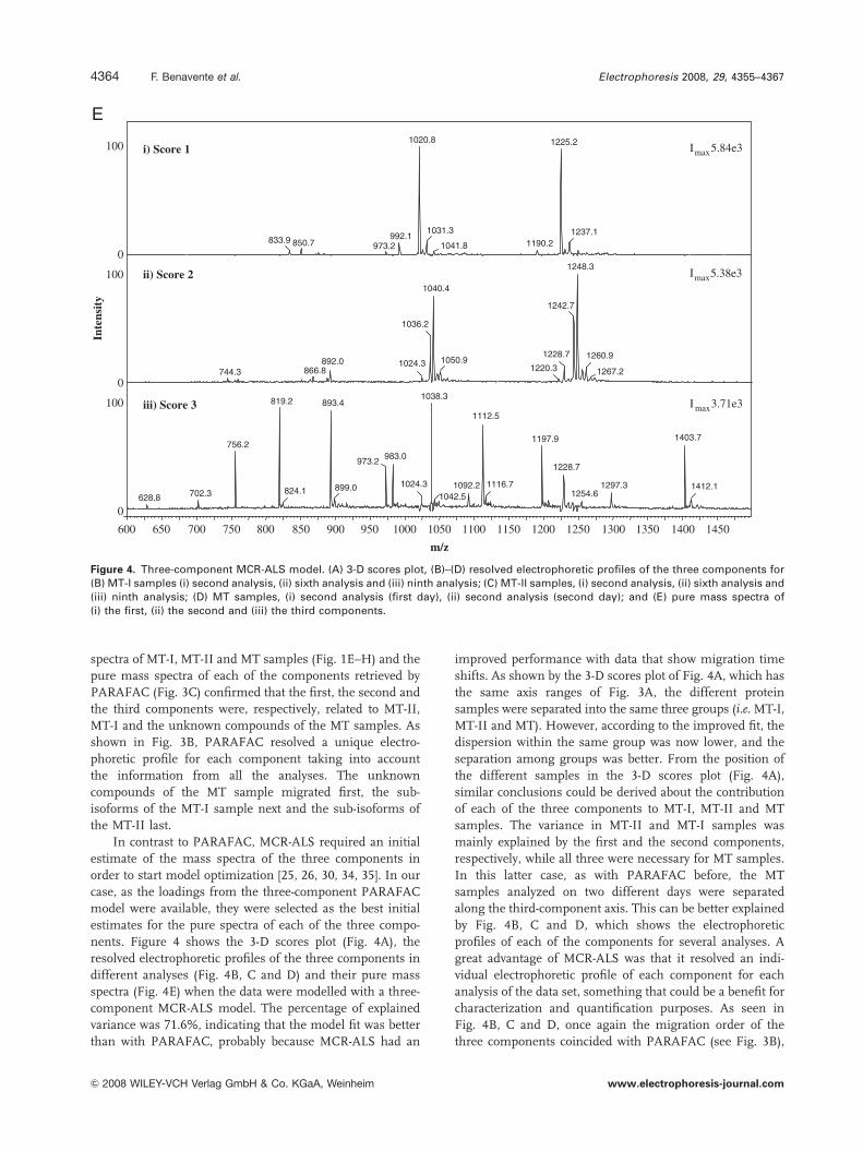
nents. Figure 4 shows the 3-D scores plot (Fig. 4A), the
resolved electrophoretic profiles of the three components in
different analyses (Fig. 4B, C and D) and their pure mass
spectra (Fig. 4E) when the data were modelled with a three-
component MCR-ALS model. The percentage of explained
variance was 71.6%, indicating that the model fit was better
than with PARAFAC, probably because MCR-ALS had an
improved performance with data that show migration time
shifts. As shown by the 3-D scores plot of Fig. 4A, which has
the same axis ranges of Fig. 3A, the different protein
samples were separated into the same three groups (i.e. MT-I,
MT-II and MT). However, according to the improved fit, the
dispersion within the same group was now lower, and the
separation among groups was better. From the position of
the different samples in the 3-D scores plot (Fig. 4A),
similar conclusions could be derived about the contribution
of each of the three components to MT-I, MT-II and MT
samples. The variance in MT-II and MT-I samples was
mainly explained by the first and the second components,
respectively, while all three were necessary for MT samples.
In this latter case, as with PARAFAC before, the MT
samples analyzed on two different days were separated
along the third-component axis. This can be better explained
by Fig. 4B, C and D, which shows the electrophoretic
profiles of each of the components for several analyses. A
great advantage of MCR-ALS was that it resolved an indi-
vidual electrophoretic profile of each component for each
analysis of the data set, something that could be a benefit for
characterization and quantification purposes. As seen in
Fig. 4B, C and D, once again the migration order of the
three components coincided with PARAFAC (see Fig. 3B),
600 650 700 750 800 850 900 950 1000 1050 1100 1150 1200 1250 1300 1350 1400 1450
0
100
0
100
0
100 I max 5.84e3
Imax5.38e3
I max3.71e3
i) Score 1
ii) Score 2
iii) Score 3
m/z
Inte
nsit
y
1020.8
992.1850.7833.9
973.2
1225.2
1031.3
1190.21041.8
1237.1
1248.3
1040.4
1036.2
892.0866.8744.3
1024.3
1242.7
1228.71050.9
1220.31260.9
1267.2
1038.3819.2
756.2
702.3628.8
893.4
824.1
983.0973.2
899.0 1024.3
1112.5
1092.21042.5
1403.71197.9
1116.7
1228.7
1297.31254.6
1412.1
E
Figure 4. Three-component MCR-ALS model. (A) 3-D scores plot, (B)–(D) resolved electrophoretic profiles of the three components for(B) MT-I samples (i) second analysis, (ii) sixth analysis and (iii) ninth analysis; (C) MT-II samples, (i) second analysis, (ii) sixth analysis and(iii) ninth analysis; (D) MT samples, (i) second analysis (first day), (ii) second analysis (second day); and (E) pure mass spectra of(i) the first, (ii) the second and (iii) the third components.
Electrophoresis 2008, 29, 4355–43674364 F. Benavente et al.
& 2008 WILEY-VCH Verlag GmbH & Co. KGaA, Weinheim www.electrophoresis-journal.com
0
1006236.5
6211.0
5198.5
4969.05174.5
5038.0
6139.0
5248.0
7484.5
7277.56298.0
7244.5
6358.0 7123.0
7453.07367.5
7558.0
Imax2.26e3
6269.54990.0
F Score 2In
tens
ity
0
1006122.0
5100.0
4896.0
4956.0
5948.0
5832.05152.0
7346.0
6182.07212.0
6938.07420.0
7494.0
I max3.54e3
6150
E Score 1
Molecular Mass (Da)
4800 5200 5600 6000 6400 6800 7200 76000
100 6668.05556.0
4910.0
4862.0
5186.0
4940.0
5116.0
5356.0
5208.05454.0
5610.0
6248.0
5984.0
5890.05834.05646.0
6140.0
6042.0
6546.0
6286.0
7012.0
6872.06806.0
7180.0
7058.0
7366.0
7262.0
7440.0
7636.07552.0
Imax958G Score 3
0
1006239.5
6213.5
5178.0
5119.0
4971.55200.0
5253.0 6100.0
6271.5
6302.56364.0
Imax5.21e5
6143.0
6174.5
Molecular Mass (Da)
A MT-I
0
1006123.0
5101.06081.5
6154.5
6671.56242.0
Imax1.06e6
6186.5
6144.0
Inte
nsit
y
B MT-II
4800 5200 5600 6000 6400 6800 7200 7600
0
1006671.5
4789.55189.0
4912.0
4971.5
5559.5
5358.5
5613.0
5731.06227.0
6034.55995.5
5837.0
6251.56549.5
6486.06480.06619.5
7265.0
7144.56810.0
6876.5
7039.56906.0
7368.5
7470.0
7716.0
IZmax1.45e5C MT-Day1
0
1006124.0
6036.0
5838.0
4912.0
5190.0
5604.0
5630.0
5996.0
5906.0
6550.0
6214.0
6252.0
6440.0
6266.06420.06362.0
7558.0
7144.06876.0
6802.06672.0
7020.0
6952.0
7462.07264.0
Imax1.16e5D MT-Day2
MT-2e
MT-2d
MT-1a
MT-1a non ac
MT-2d non ac
6200.0MT-2e non ac
MT-2a
MT-2b
MT-2c
MT-2a non ac
MT-2e
MT-2d
MT-1a
6142.1
MT-2a
MT-2b
MT-2c
Figure 5. Mass spectra deconvoluted from the raw ESI mass spectra of Fig. 1A–D, (A) MT-I, (B) MT-II, (C) MT (first day) and (D) MT(second day) samples. Mass spectra deconvoluted from the pure mass spectra of the three components of the MCR-ALS model (E) firstcomponent, (F) second component and (G) third component.
Electrophoresis 2008, 29, 4355–4367 CE and CEC 4365
& 2008 WILEY-VCH Verlag GmbH & Co. KGaA, Weinheim www.electrophoresis-journal.com
and it was clear that the variance of MT-I and MT-II samples
was mainly explained by the second and the first compo-
nents respectively, while all three were necessary for MT
samples. Furthermore, the electrophoretic profiles of the
three components within the same group of samples were
similar, even for the MT samples analyzed on two different
days (Fig. 4D). The separation of MT samples into two
groups in the 3-D scores plot of Fig. 4A could be tentatively
explained by the differences in the ranges of the y-axis of
Fig. 4D plots, which were due to the lower S/N ratio of the
CE-ESI-MS electropherograms acquired for the MT samples
during the second day (see the TIE of Fig. 1C and D). In this
sense, the quantitative information that can be extracted
from the electrophoretic profiles resolved by MCR-ALS
allowed improved sample characterization. Figure 4E shows
the pure mass spectra of each of the components retrieved
with MCR-ALS, which were identical to those obtained with
PARAFAC (Fig. 3C). This confirmed the goodness of the
pure mass spectra obtained by PARAFAC, which were an
excellent alternative for initializing MCR-ALS optimization.
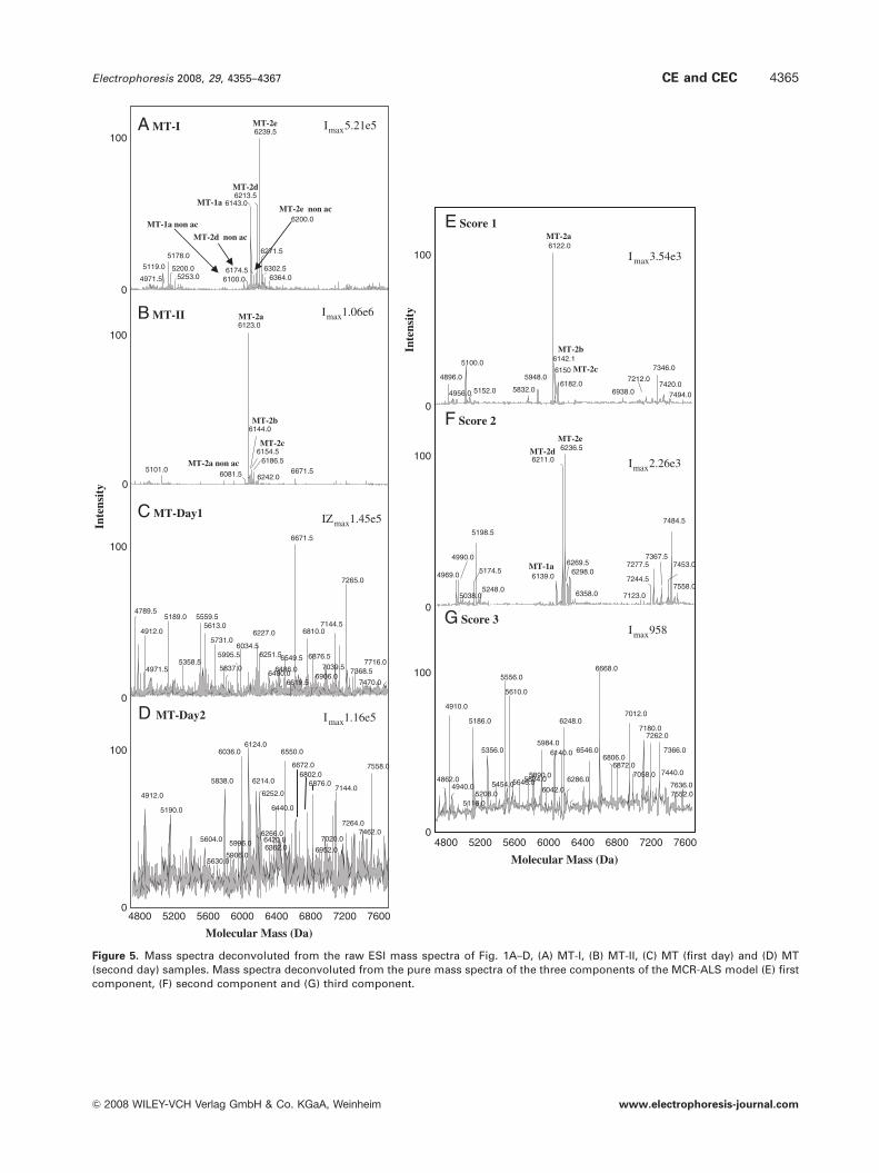
Figure 5A–D shows the zero charge mass spectra
deconvoluted from the ESI mass spectra of Fig. 1E–H. In a
similar way, Fig. 5E–G shows those obtained from the pure
mass spectra of each of the three MCR-ALS components.
Consistent with the TIE of Fig. 1A and B and Table 1, the
Mm values of MT-1a, MT-2d, MT-2e, MT-1a non-ac, MT-2d
non-ac and MT-2e non-ac were observed in the deconvoluted
mass spectra of the MT-I sample (Fig. 5A) and those of
MT-2a, MT-2b, MT-2c and MT-2a non-ac were found in the
deconvoluted mass spectra of the MT-II sample (Fig. 5B).
The other Mm values, which as explained before were
difficult to unambiguously identify, could be tentatively
attributed to some degradation products or oxidized MT sub-
isoforms [6, 37]. However, from the point of view of a
multivariate data analysis, the Mm information from the
unidentified compounds is also useful as part of the indi-
vidual fingerprint of each MT-I, MT-II and MT sample. As
the first and the second components were related with
MT-II and MT-I samples, respectively, their deconvoluted
mass spectra (Fig. 5E and F) contained most of the infor-
mation observed in the deconvoluted mass spectra of MT-II
and MT-I samples (Fig. 5B and A), respectively. In addition,
there were some other minor signals, because both
components were also explaining to some extent the
variance of the rest of the data set. With reference to
the information related with MT-II and MT-I samples in the
first and the second components (Fig. 5E and F, respec-
tively), it was possible to clearly identify the Mm values of
the most-abundant sub-isoforms, which differed by only a
few mass units (1–4 Da) from the Mm values obtained for
MT-I and MT-II samples (Fig. 5A and B). The accuracy of
the Mm values obtained with MCR-ALS or PARAFAC will
have important implications when an reliable identification
is necessary, and it could be improved by using an MS
detector with improved mass accuracy and resolution [9].
However, at this point, it is important to emphasize the
excellent accuracy of the Mm data obtained from both
multivariate data analysis models. In accordance with the
ESI mass spectra of Fig. 1G and H, the deconvoluted mass
spectra of the MT samples were more complex and noisy
(Fig. 5C and D). Again, it was difficult to observe from visual
inspection whether the MT sample contained, among other
compounds, the sub-isoforms found in MT-I and MT-II
samples. In a similar way, it was complicated to assert
whether the deconvoluted mass spectra of the MT samples
(Fig. 5C and D) contained the information retrieved by the
deconvoluted mass spectra of the three components
(Fig. 5E–G). However, all the results discussed above ensure
that the pure spectra retrieved by MCR-ALS were repre-
sentative of the compounds in the MT-I, MT-II and MT
samples and that the Mm values obtained from the decon-
voluted mass spectra could be used for identification and
confirmation purposes.
4 Concluding remarks
Multivariate data analysis based on PARAFAC and MCR-
ALS models have demonstrated to be excellent complemen-
tary tools with which to investigate, in a direct way and with
minimum prior knowledge, the highly complex and over-
lapping electrophoretic profiles that are usually obtained by
CE-ESI-MS for protein isoforms. Using both methods it was
possible to discriminate a characteristic fingerprint for MT-I,
MT-II and MT samples, based on the electrophoretic
profiles and the pure mass spectra of the three model
components, which contributed in a different way to
explaining the variance of each protein type. For MT-I
and MT-II samples it was also possible to identify the
Mm values of their main characteristic sub-isoforms after
deconvolution of the pure mass spectra of their specific
model component. The results with MCR-ALS in terms of
classification were slightly better than those obtained with
PARAFAC, because it performed better with the pre-
processed electropherograms, which showed small migra-
tion time shifts. However, no differences were found
between the pure mass spectra of the three components
for either model. MCR-ALS allowed us to resolve an
individual electrophoretic profile of each of the three
components for each of the analyzed samples, something
that was advantageous for characterization and quantifica-
tion purposes. The application of multivariate data analysis
methods to protein isoform separation and characterization
should be regarded as an efficient, novel alternative for
achieving a deeper understanding of the vast amount of data
obtained by hyphenated techniques for the analysis of
complex proteins.
B. A. is grateful to the University of Barcelona for awardinga doctoral fellowship. This study was supported in part by a grantfrom the Spanish Ministry of Science and Technology(CTQ2005-04357/BQU).
The authors have declared no conflict of interest.
Electrophoresis 2008, 29, 4355–43674366 F. Benavente et al.
& 2008 WILEY-VCH Verlag GmbH & Co. KGaA, Weinheim www.electrophoresis-journal.com

5 References
[1] Haselberg, R., de Jong, G. J., Somsen, G. W. J.Chromatogr. A 2007, 1159, 81–109.
[2] Hernandez-Borges, J., Neussus, C., Cifuentes, A.,Pelzing, M., Electrophoresis 2004, 25, 2257–2281.
[3] Klampfl, C. W., Electrophoresis 2006, 27, 3–34.
[4] Stutz, H., Electrophoresis 2005, 26, 1254–1290.
[5] Sanz-Nebot, V., Benavente, F., Vallverdu, A., Guzman,N. A., Barbosa, J., Anal. Chem. 2003, 75, 5220–5229.
[6] Andon, B., Barbosa, J., Sanz-Nebot, V., Electrophoresis2006, 27, 3661–3670.
[7] Sanz-Nebot, V., Balaguer, E., Benavente, F., Neussus, C.,Barbosa, J., Electrophoresis 2007, 28, 1949–1957.
[8] Prange, A., Profrock, D., Anal. Bioanal. Chem. 2005, 383,372–389.
[9] Balaguer, E., Demelbauer, U. M., Pelzing, M., Sanz-Nebot,V. et al., Electrophoresis 2006, 27, 2638–2650.
[10] Sentellas, S., Saurina, J., J. Sep. Sci. 2003, 26,1395–1402.
[11] Booksh, K. S., Kowalski, B. R., Anal. Chem. 1994, 66,782A–791A.
[12] Benavente, F., Gimenez, E., Olivieri, A. C., Barbosa, J.,Sanz-Nebot, V., Electrophoresis 2006, 27, 4008–4015.
[13] Kaiser, T., Wittke, S., Just, I., Krebs, R. et al., Electro-phoresis 2004, 25, 2044–2055.
[14] Ullsten, S., Danielsson, R., Backstrom, D., Sjoberg, P.,Bergquist, J., J. Chromatogr. A 2006, 1117, 87–93.
[15] Gonzalez-Duarte, P., in: McCleverty (Ed.), Metallothioneins,Comprehensive Coordination Chemistry II, vol. 8, Elsevier,Oxford 2004, pp. 213–228.
[16] Stillman, M. J., Coord. Chem. Rev. 1995, 144,461–511.
[17] Nordberg, M., Talanta 1998, 46, 243–254.
[18] Klaasen, C. D., Liu, J., Choudhuri, S., Annu. Rev.Pharmacol. Toxicol. 1999, 39, 267–294.
[19] Nordberg, G., Jin, T., Leffler, P., Svensson, M.,Nordberg, M., Analysis 2000, 28, 396–400.
[20] Cosson, R. P. Amiard, J. C., in: Lagadic, L. et al. (Eds.),Use of Biomarkers for Environmental Quality Assess-ment, Science Publishers, Enfield 2000, pp. 79–111.
[21] Kojima, Y., Meth. Enzymol. 1991, 205, 8–10.
[22] Andersen, C. M., Bro, R., J. Chemom. 2003, 17, 200–215.
[23] Bro, R., Chemom. Intell. Lab. Syst. 1997, 38, 149–171.
[24] Paatero, P., Chemom. Intell. Lab. Syst. 1997, 38,223–242.
[25] Tauler, R., Chemom. Intell. Lab. Syst. 1995, 30, 133–146.
[26] Tauler, R., Smilde, A., Kowalski, B., J. Chemom. 1995, 9,31–58.
[27] Husheer, S. L. G., Forest, O., Henderson, M., McIndoe,J. S., Rapid Commun. Mass Spectrom. 2005, 19,1352–1354.
[28] Vargas, C. A., moving_average2, http://www.mathworks.com/matlabcentral/fileexchange.
[29] Andersson, C. A., Bro, R., Chemom. Intell. Lab. Syst.2000, 52, 1–4.
[30] Jaumot, J., Gargallo, R., de Juan, A., Tauler, R.,Chemom. Intell. Lab. Syst. 2005, 76, 101–110.
[31] Wang, J., Bose, S., Hage, D. S., J. Chromatogr. A 1996,735, 209–220.
[32] Munoz de la Pena, A., Espinosa-Mansilla, A., Gonzalez-Gomez, D., Olivieri, A. C., Goicoechea, H. C., Anal.Chem. 2003, 75, 2640–2646.
[33] Braga, J. W. B., Bottoli, C. B. G., Jardim, I. C. S. F.,Goicoechea, H. C. et al., J. Chromatogr. A 2007, 1148,200–210.
[34] Pere-Trepat, E., Lacorte, S., Tauler, R., Anal. Chim. Acta2007, 595, 228–237.
[35] Jaumot, J., Tauler, R., Gargallo, R., Anal. Biochem.2006, 358, 76–89.
[36] Hunziker, P. E., Kaur, P., Wan, M., Kanzig, A., Biochem.J. 1995, 306, 265–270.
[37] Sanz-Nebot, V., Andon, B., Barbosa, J., J. Chromatogr.B 2003, 796, 379–393.
[38] Tomasi, G., van den Berg, F., Andersson, C.,J. Chemom. 2004, 18, 231–241.
Electrophoresis 2008, 29, 4355–4367 CE and CEC 4367
& 2008 WILEY-VCH Verlag GmbH & Co. KGaA, Weinheim www.electrophoresis-journal.com
Top Related
Copyright © 2022 FDOKUMEN

