


Bahasa
Halaman
Hukum

A Label Semantics Approach to Linguistic Hedges
Martha Lewis and Jonathan LawryDepartment of Engineering Mathematics,
University of Bristol,BS8 1TR, United Kingdom
[email protected], [email protected]
28th January 2014
Abstract
We introduce a model for the linguistic hedges ‘very’ and ‘quite’ within the label semantics frame-work, and combined with the prototype and conceptual spaces theories of concepts. The proposed modelemerges naturally from the representational framework we use and as such, has a clear semantic ground-ing. We give generalisations of these hedge models and show that they can be composed with themselvesand with other functions, going on to examine their behaviour in the limit of composition.
1 Introduction
The modelling of natural language relies on the idea that languages are compositional, i.e. that the meaningof a sentence is a function of the meanings of the words in the sentence, as proposed by [13]. Whether ornot this principle tells the whole story, it is certainly important as we undoubtedly manage to create andunderstand novel combinations of words. Fuzzy set theory has long been considered a useful framework forthe modelling of natural language expressions, as it provides a functional calculus for concept combination[30, 32].
A simple example of compositionality is hedged concepts. Hedges are words such as ‘very’, ‘quite’, ‘moreor less’, ‘extremely’. They are usually modelled as transforming the membership function of a base conceptto either narrow or broaden the extent of application of that concept. So, given a concept ‘short’, theterm ‘very short’ applies to fewer objects than ‘short’, and ‘quite short’ to more. Modelling a hedge as atransformation of a concept allows us to determine membership of an object in the hedged concept as afunction of its membership in the base concept, rather than building the hedged concept from scratch [31].
Linguistic hedges have been widely applied, including in fuzzy classifiers [6, 7, 20, 22] and databasequeries [1, 3]. Using linguistic hedges in these applications allows increased accuracy in rules or querieswhilst maintaining human interpretability of results [4, 23]. This motivates the need for a semanticallygrounded account of linguistic hedges: if hedged results are more interpretable then the hedges used mustthemselves be meaningful.
In the following we provide an account of linguistic hedges that is both functional, and semanticallygrounded. In its most basic formulation, the operation requires no additional parameters, although wealso show that the formulae can be generalised if necessary. Our account of linguistic hedges uses thelabel semantics framework to model concepts [17]. This is a random set approach which quantifies anagent’s subjective uncertainty about the extent of application of a concept. We refer to this uncertainty assemantic uncertainty [19] to emphasise that it concerns the definition of concepts and categories, in contrastto stochastic uncertainty which concerns the state of the world. In [19] the label semantics approach iscombined with conceptual spaces [14] and prototype theory [25], to give a formalisation of concepts as basedon a prototype and a threshold, located in a conceptual space. This approach is discussed in detail in section2. An outline of the paper is then as follows: section 3 discusses different approaches to linguistic hedges
1
from the literature, and compares these with our model. Subsequently, in section 4, we give formulations ofthe hedges ‘very’ and ‘quite’. These are formed by considering the dependence of the threshold of a hedgedconcept on the threshold of the original concept. We give a basic model and two generalisations, show thatthe models can be composed and investigate the behaviour in the limit of composition. Section 5 comparesour results to those in the literature and proposes further lines of research.
2 Theoretical approach to concepts
2.1 Prototype theory and fuzzy set theory
Prototype theory views concepts as being defined in terms of prototypes, rather than by a set of necessaryand sufficient conditions. Elements from an underlying metric space then have graded membership in aconcept depending on their similarity to a prototype for the concept. There is some evidence that humansuse natural categories in this way, as shown in experiments reported in [25]. Fuzzy set theory [30] wasproposed as a calculus for combining and modifying concepts with graded membership, and extended theseideas in [32] to linguistic variables as variables taking words as values, rather than numbers. For example,‘height’ can be viewed as a linguistic variable taking values ‘short,’ ‘tall’, ‘very tall’, etc. The variable relatesto an underlying universe of discourse Ω, which for the concept ‘tall’ could be R+. Then each value L of thevariable is associated with a fuzzy subset of Ω, and a function µL : Ω → [0, 1] associates with each x ∈ Ωthe value of its membership in L. Prototype theory gives a semantic basis to fuzzy sets through the notionof similarity to a prototype, as described in [10]. In this context, concepts are represented by fuzzy sets andmembership of an element in a concept is quantified by its similarity to the prototype. In this situation thefuzziness of the concept is seen as inherent to the concept. An alternative interpretation for fuzzy sets israndom set theory, see [10] for an exposition. Here, the fuzziness of a set comes from uncertainty about acrisp set, i.e. semantic uncertainty, rather than fuzziness inherent in the world. This second approach is thestance taken by [19], and which we now adopt in this paper.
2.2 Conceptual Spaces
Conceptual spaces are proposed by Gardenfors in [14] as a framework for representing information at theconceptual level. Gardenfors contrasts his theory with both a symbolic, logical approach to concepts, andan associationist approach where concepts are represented as associations between different kinds of basicinformation elements. Rather, conceptual spaces are geometrical structures based on quality dimensionssuch as weight, height, hue, brightness, etc. It is assumed that conceptual spaces are metric spaces, withan associated distance measure. This might be Euclidean distance, or any other appropriate metric. Thedistance measure can be used to formulate a measure of similarity, as needed for prototype theory - similarobjects are close together in the conceptual space, very different objects are far apart.
To develop the conceptual space framework, Gardenfors also introduces the notion of integral and sepa-rable dimensions. Dimensions are integral if assignment of a value in one dimension implies assignment ofa value in another, such as depth and breadth. Conversely, separable dimensions are those where there isno such implication, such as height and sweetness. A domain is then defined as a set of quality dimensionsthat are separable from all other dimensions, and a conceptual space is defined as a collection of one or moredomains.
Gardenfors goes on to define a property as a convex region of a domain in a conceptual space. A conceptis defined as a set of such regions that are related via a set of salience weights. This casting of (at least)properties as convex regions of a domain sits very well with prototype theory, as Gardenfors points out. Ifproperties are convex regions of a space, then it is possible to say that an object is more or less central tothat region. Because the region is convex, its centroid will lie within the region, and this centroid can beseen as the prototype of the property.
2
2.3 Label Semantics
The label semantics framework was proposed by [17] and related to prototype theory and conceptual spacesin [19]. In this framework, agents use a set of labels LA = L1, L2, ..., Ln to describe an underlyingconceptual space Ω which has a distance metric d(x, y) between points. In fact, it is sufficient that d(x, y)be a pseudo-distance. When x or y is a set, say Y , we take d(x, Y ) = mind(x, y) : y ∈ Y . In this case, theset Y is seen as an ontic set, i.e., a set where all elements are jointly prototypes, as opposed to an epistemicset describing a precise but unknown prototype, as described in [11]. Each label Li is associated with firstlya set of prototype values Pi ⊆ Ω, and secondly a threshold εi, about which the agents are uncertain. Thethresholds εi are drawn from probability distributions δεi . Labels Li are associated with neighbourhoodsN εiLi
= x ∈ Ω : d(x, Pi) ≤ εi. The neighbourhood can be seen as the extension of the concept Li. Theintuition here is that εi captures the idea of being sufficiently close to prototypes Pi. In other words, x ∈ Ωis sufficiently close to Pi to be appropriately labelled as Li providing that d(x, Pi) ≤ εi.
Given an element x ∈ Ω, we can ask how appropriate a given label is to describe it. This is quantifiedby an appropriateness measure, denoted µLi
(x). We are intentionally using the same notation as for themembership function of a fuzzy set. This quantity is the probability that the distance from x to Pi, theprototype of Li, is less than the threshold εi, as given by:
µLi(x) = P (εi : x ∈ N εi
Li) = P (εi : d(x, Pi) ≤ εi) =
∫ ∞d(x,Pi)
δεi(εi)dεi
We also use the notation∫∞dδεi(εi)dεi = ∆i(d), according to which µLi(x) = ∆i(d(x, Pi)). The above
formulation provides a link to the random set interpretation of fuzzy sets. Random sets are random variablestaking sets as values. If we viewN εi
Lias a random set from R+ into 2Ω, then µLi
(x) is the single point coveragefunction of N εi
Li, as defined in [18], and also commonly called a contour function [26].
Labels can often be semantically related to each other. For example, the label ‘pet fish’ is semanticallyrelated to the labels ‘pet’ and ‘fish’, and the label ‘very tall’ related to the label ‘tall’. This prompts twoquestions: firstly, how the prototypes of each concept are related to each other, and secondly, how thethresholds of each concept are related. Two simple models for the relationships between the thresholds aregiven in [19]. The consonant model takes all thresholds as being dependent on one common underlyingthreshold. So, all thresholds have the same distance metric d and are related to a base threshold ε bythe dependency that εi = fi(ε) for increasing functions fi. In contrast, the independence model takesall thresholds as being independent of each other. This might hold when labels are taken from differentconceptual spaces.
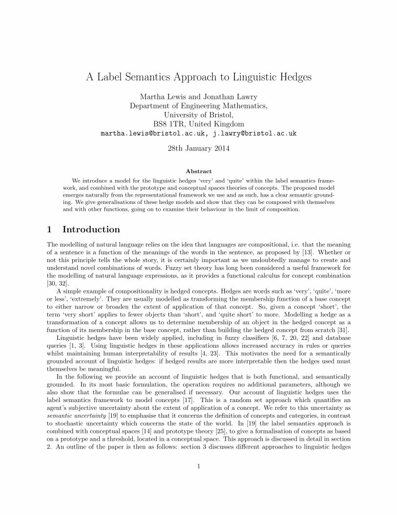
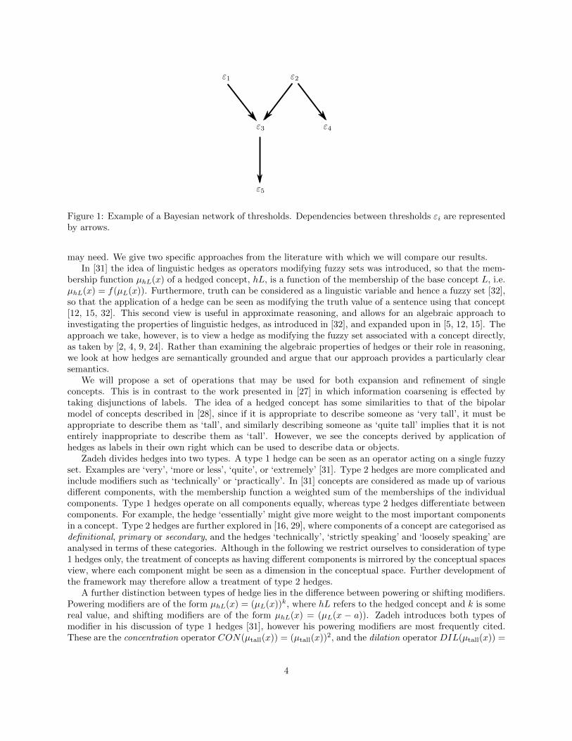
Between these two extremes, we model dependencies between thresholds as a Bayesian network - i.e., adirected acyclic graph whose edges encode conditional dependence between variables. The key property ofthis type of network is that the joint distribution of all variables can be broken into factors that depend onlyon each individual variable and its parents. So, for example, the network in figure 1 can be factorised asδ(ε1, ε2, ε3, ε4, ε5) = δε1(ε1)δε2(ε2)δε3|ε1,ε2(ε3|ε1, ε2)δε4|ε2(ε4|ε2)δε5|ε3(ε5|ε3).
This enables calculation of the joint distribution and therefore marginal distributions in an efficientmanner.
One intuitively easy example is where the dependency of one threshold ε2 on another ε1 is that ε2 ≤ ε1.This could be taken to model the dependency of the threshold of the concept ‘very tall’ on the threshold of‘tall’. The label ‘very tall’ should be appropriate to describe fewer people than the label ‘tall’. Therefore, thethreshold for describing someone as ‘very tall’ will be narrower than the threshold for describing someone as‘tall’, i.e. εvery tall ≤ εtall. This simple model will form part of the approach to modelling linguistic hedges,as outlined in the sequel.
3 Approaches to linguistic hedges
Linguistic hedges have been given varying treatments in the literature. In this section we summarise thesedifferent approaches and state the approach that we wish to take, discussing properties that hedge modifiers
3
ε2ε1
ε3
ε5
ε4
1
Figure 1: Example of a Bayesian network of thresholds. Dependencies between thresholds εi are representedby arrows.
may need. We give two specific approaches from the literature with which we will compare our results.In [31] the idea of linguistic hedges as operators modifying fuzzy sets was introduced, so that the mem-
bership function µhL(x) of a hedged concept, hL, is a function of the membership of the base concept L, i.e.µhL(x) = f(µL(x)). Furthermore, truth can be considered as a linguistic variable and hence a fuzzy set [32],so that the application of a hedge can be seen as modifying the truth value of a sentence using that concept[12, 15, 32]. This second view is useful in approximate reasoning, and allows for an algebraic approach toinvestigating the properties of linguistic hedges, as introduced in [32], and expanded upon in [5, 12, 15]. Theapproach we take, however, is to view a hedge as modifying the fuzzy set associated with a concept directly,as taken by [2, 4, 9, 24]. Rather than examining the algebraic properties of hedges or their role in reasoning,we look at how hedges are semantically grounded and argue that our approach provides a particularly clearsemantics.
We will propose a set of operations that may be used for both expansion and refinement of singleconcepts. This is in contrast to the work presented in [27] in which information coarsening is effected bytaking disjunctions of labels. The idea of a hedged concept has some similarities to that of the bipolarmodel of concepts described in [28], since if it is appropriate to describe someone as ‘very tall’, it must beappropriate to describe them as ‘tall’, and similarly describing someone as ‘quite tall’ implies that it is notentirely inappropriate to describe them as ‘tall’. However, we see the concepts derived by application ofhedges as labels in their own right which can be used to describe data or objects.
Zadeh divides hedges into two types. A type 1 hedge can be seen as an operator acting on a single fuzzyset. Examples are ‘very’, ‘more or less’, ‘quite’, or ‘extremely’ [31]. Type 2 hedges are more complicated andinclude modifiers such as ‘technically’ or ‘practically’. In [31] concepts are considered as made up of variousdifferent components, with the membership function a weighted sum of the memberships of the individualcomponents. Type 1 hedges operate on all components equally, whereas type 2 hedges differentiate betweencomponents. For example, the hedge ‘essentially’ might give more weight to the most important componentsin a concept. Type 2 hedges are further explored in [16, 29], where components of a concept are categorised asdefinitional, primary or secondary, and the hedges ‘technically’, ‘strictly speaking’ and ‘loosely speaking’ areanalysed in terms of these categories. Although in the following we restrict ourselves to consideration of type1 hedges only, the treatment of concepts as having different components is mirrored by the conceptual spacesview, where each component might be seen as a dimension in the conceptual space. Further development ofthe framework may therefore allow a treatment of type 2 hedges.
A further distinction between types of hedge lies in the difference between powering or shifting modifiers.Powering modifiers are of the form µhL(x) = (µL(x))k, where hL refers to the hedged concept and k is somereal value, and shifting modifiers are of the form µhL(x) = (µL(x − a)). Zadeh introduces both types ofmodifier in his discussion of type 1 hedges [31], however his powering modifiers are most frequently cited.These are the concentration operator CON(µtall(x)) = (µtall(x))2, and the dilation operator DIL(µtall(x)) =
4
(µtall(x))12 , which are often taken to implement the hedges ‘very’ and ‘quite’, (alternatively ‘more or less’),
respectively. 1
The operators CON and DIL leave the core, x ∈ Ω : µL(x) = 1, and support x ∈ Ω : µL(x) 6= 0, ofthe fuzzy sets unchanged, which is often argued to be undesirable [3, 2, 24, 21]. In particular, [3] argue that ina fuzzy database, if a concentrating hedge is being used to refine a query that is returning too many objects,the hedge needs to reduce the number of objects returned, and hence narrow down the core. Furthermore,[22] find that classifiers using the CON and DIL operators (classical hedges) do not perform as well as thosewith hedges that modify the core and support of the fuzzy sets. In contrast, Zadeh himself argues that thecore should not be altered. The application of a modifier ‘very’ to a property given by a crisp set shouldleave that property unchanged: ‘very square’ is the same as ‘square’. A fuzzy set is made up of a non-fuzzypart, the core, and a fuzzy part, x ∈ Ω : 0 < µL(x) < 1. Since the core of a fuzzy set is a crisp set, itshould be left unchanged. The use of classical hedges does improve performance over non-hedged fuzzy rulesin expert systems [6, 7, 20], so the argument against classical hedges is a matter of degree.
The use of the CON and DIL operators to model the hedges ‘very’ and ‘quite’ is further criticised onthe basis that the modifiers are arbitrary and semantically ungrounded. No justification is given for thesemodifiers other than that they have what seem to be intuitively the right properties [2, 8, 24]. Groundinghedges semantically is important for a theoretical account of what happens when we use terms like ‘very’and also for retaining interpretability in fuzzy systems. [2, 8] both ground modifiers using a resemblancerelation which takes into account how objects in the universe are similar to each other. [24] takes a horizonshifting approach.
In [24] the class of finite numbers is used as an example of the horizon shifting approach. Some numbersare certainly finite, however as numbers get larger, finiteness becomes impossible to verify. Mapping thisidea onto the concept ‘small’, we can say that there is a class of numbers that are definitely small, say [0, c].As numbers get larger than c we approach the horizon past which the concept ‘small’ no longer applies,expressed as 1− ε(x)(x− c). So:
µsmall(x) =
1 if x ∈ [0, c]
1− ε(x)(x− c) if x ≥ cNow, to implement the hedge ‘very’, the horizon c is shifted by a factor σ and the membership function
altered thus:
µvery small(x) =
1 if x ∈ [0, σc]
1− ε(x, σ)(x− σc) if x ≥ σcIn [24], examples of different kinds of membership functions that might be used to implement this idea
are given. A linear membership function gives ε(x) = 1a−c where a is the upper limit of the membership
function. To implement the hedge, the function ε(x, σ) = 1σ(a−c) is introduced, giving
µsmall(x) =
1 if x ∈ [0, c]
1− x−ca−c if x ∈ [c, a]
0 otherwise
and
µvery small(x) =
1 if x ∈ [0, σc]
1− x−σcσ(a−c) if x ∈ [σc, σa]
0 otherwise
[2, 8] both ground their approaches in the idea of looking at the elements near a fuzzy set in orderto contract or dilate the set. The two approaches are similar, so we restrict ourselves to that of [2]. This
1Zadeh in fact proposes a rather more complicated hedge for ‘more or less’, which involves a combination of powering andshifting, however, the dilation operator is more frequently quoted in the literature.
5
approach introduces a fuzzy resemblance relation on the universe of discourse, and either a T -norm in the caseof dilation, or a fuzzy implicator for concentration. The modifier is then implemented as follows. Consider afuzzy set F and a proximity relation EZ which is approximate equality, parametrised by a fuzzy set Z. Asdescribed in [2], E is modelled by (u, v)→ E(u, v) = Z(u− v), where Z is a fuzzy interval centred on 0 withfinite support. In terms of a trapezoidal membership function, Z can be expressed as (−z − a,−z, z, z + a).Therefore, if |u − v| ≤ z, u and v are judged to be approximately equal, i.e. EZ(u, v) = 1. The set F isdilated by EZ(F )(s) = supr∈ΩT (F (r), EZ(s, r)), where T is any T -norm, min being the standard.
To understand the effect that this has on a fuzzy set F , suppose that F has a trapezoidal membershipfunction (A,B,C,D) where [B,C] is the core of F and [A,B], [C,D] the support, and that Z similarly is(−z − a,−z, z, z + a), with the T-norm min used. Then EZ(F ) = (A− z − a,B − z, C + z,D + z + a).
Concentration is effected in a similar way: EZ(F )(s) = infr∈ΩI(F (r), EZ(s, r)), where I is a fuzzyimplication. If F and Z are as above with the condition that C − B ≥ 2z, and I is the Godel implication,then EZ(F ) = (A+ z + a,B + z, C − z,D − z − a).
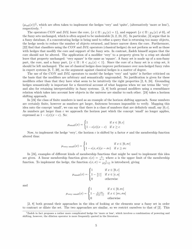
For example, suppose we start with a set F described in trapezoidal notation as F = (A,B,C,D) =(2, 4, 6, 8), and an approximate equality function parametrised by Z = (−z−a,−z, z, z+a) = (−1,−0.5, 0.5, 1).The dilation of the set F using T-norm min is then:
EZ(F ) = (A− z − a,B − z, C + z,D + z + a) = (1, 3.5, 6.5, 9)
The concentration of the set F using the Godel implication is:
EZ(F ) = (A+ z + a,B + z, C − z,D − z − a) = (3, 4.5, 5.5, 7)
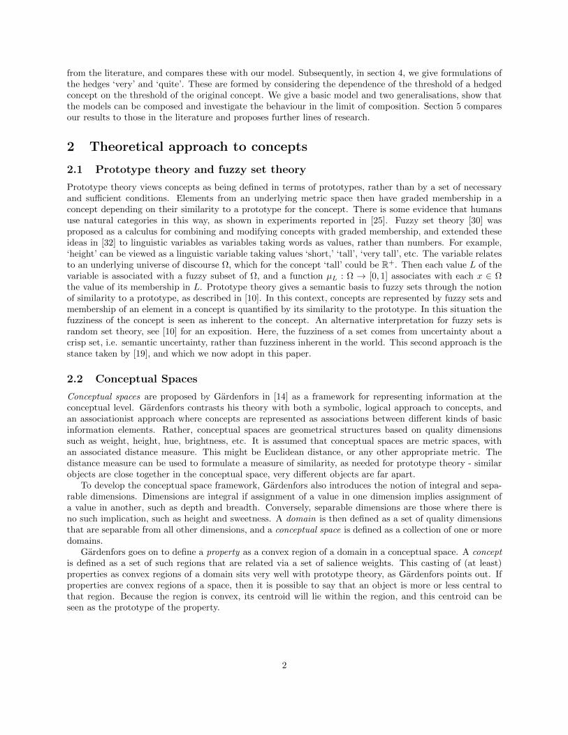
These effects are illustrated in figure 2.
0 2 4 6 8 100
0.2
0.4
0.6
0.8
1
s
F
F
EZ(F)
EZ(F)
Figure 2: Illustration of the expansion and contraction modifiers proposed in [2]. The original set F canbe described in trapezoidal set notation as (2, 4, 6, 8). The approximate equality function is parametrisedby a set Z = (−1,−0.5, 0.5, 1). Dilating the set as described in [2] gives the set EZ(F ) = (1, 3.5, 6.5, 9).Concentrating the set as described results in the set EZ(F ) = (3, 4.5, 5.5, 7)
The intuitive idea behind this approach is that if an object x1 resembles another object x2 that is L,then x1 can be said to be ‘quite L’. Conversely, object x2 that is L can be said to be ‘very L’ only if allthe objects x that resemble it can be said to be L. This formulation alters both the core and support of thefuzzy set L, which has been argued to be a desirable effect.
Following [2, 8, 24], we will propose linguistic modifiers that are semantically grounded rather thanattempting to show their utility in classifiers, reasoning or to examine the algebra of modifiers. Our approachto linguistic modifiers arises very naturally from the label semantics framework, and the primary result doesnot require any parameters additional to the original membership function of the concept. We also showsimilarities between our model and the two detailed above.
6
ε1
ε2 ≥ ε1
ε21
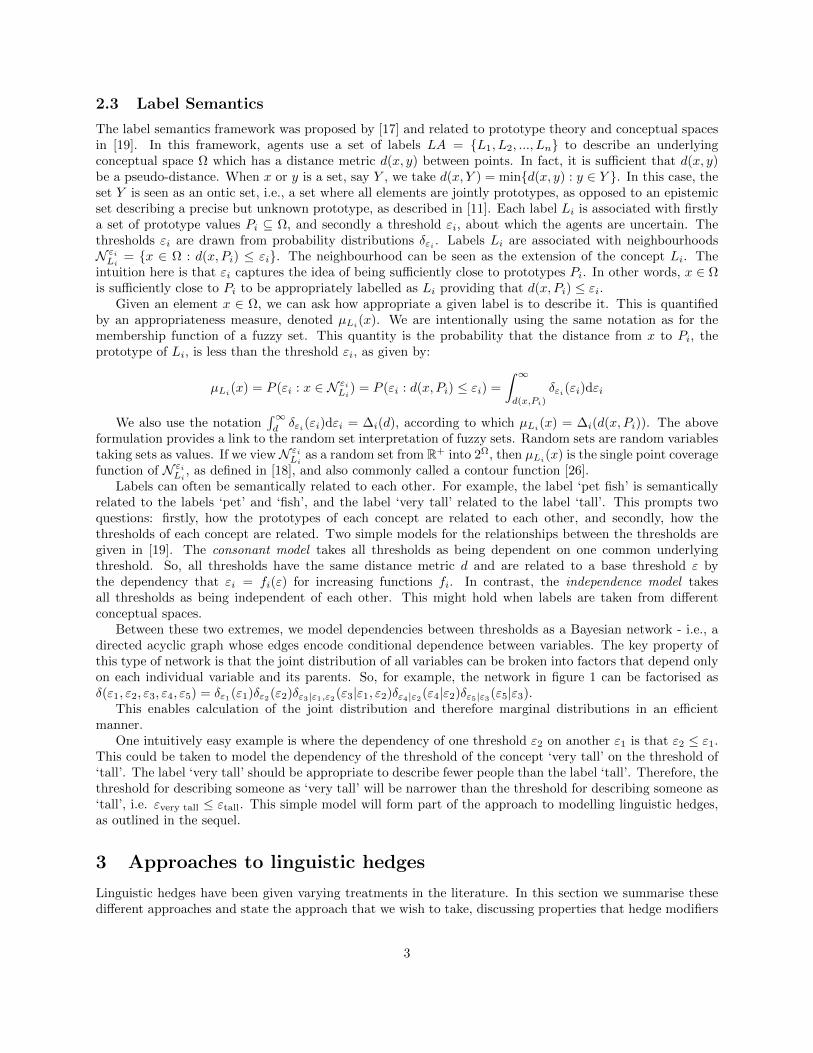
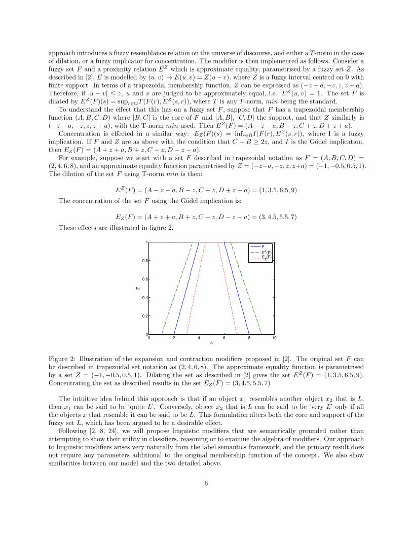
Figure 3: Directed acyclic graph representing the hedge ‘quite’. The threshold ε2 is dependent on thethreshold ε1 by ε2 ≥ ε1.
4 Label semantics approach to linguistic hedges
We present three formulations of linguistic hedges with increasing levels of generality. The first assumesthat prototypes are equal. Secondly, we show that an analogue holds where prototypes are not equal, andthirdly that these hold in the case where the second threshold is a function of the first. We go on to showsimilarities between our model and those of [2, 8, 24]. Furthermore, we show that hedges are compositional,and look at their behaviour in the limit of composition.
As described in section 2.3, LA denotes a finite set of labels Li that agents use to describe basiccategories. Ω is the underlying domain of discourse, with prototypes Pi ∈ Ω and thresholds εi, drawn froma distribution δεi . As before, the appropriateness µLi
(x) = ∆i(d(x, Pi)) =∫∞d(x,Pi)
δεi(εi)dεi. We use the
notation Li =< Pi, d, δεi >.A concept L1 can be narrowed or broadened to a second concept L2 using the linguistic hedges ‘very’ and
‘quite’ respectively, i.e. L2 is defined as ‘quite L1’. The directed acyclic graph illustrating this dependencyis given in figure 3. In this case, the threshold ε2 associated with L2 is dependent on ε1 in that ε2 ≥ ε1. Inthe case of ‘very’, we have that ε2 ≤ ε1. Essentially, for ‘quite’, we are saying that however wide a marginof certainty we apply the label ‘tall’ with, the margin for ‘quite tall’ will be wider, and conversely for ‘very’.
4.1 Hedges with unmodified prototypes
Definition 1 (Dilation and Concentration). A label L2 =< P2, d, δε2 > is a dilation of a label L1 =<P1, d, δε1 > when ε2 is dependent on ε1 such that ε2 ≥ ε1. L2 is a concentration of L1 when ε2 is dependenton ε1 such that ε2 ≤ ε1.
Theorem 2 (L2 = quite L1). Suppose L2 =< P2, d, δε2 > is a dilation of L1 =< P1, d, δε1 >, so thatε2 ≥ ε1. Suppose also that P1 = P2 = P , and that the marginal (unconditional) distribution of ε2, beforeconditioning on the knowledge that ε2 ≥ ε1, is identical to δε1 , since L2 is a dilation of L1. Then ∀x ∈ Ω,µL2
(x) = µL1(x)− µL1
(x) ln(µL1(x)).
Proof.
δε2|ε1(ε2|ε1) =
δε1 (ε2)∫∞ε1δε1 (ε2)dε2
if ε2 ≥ ε1
0 otherwise=
δε1 (ε2)
∆1(ε1) if ε2 ≥ ε1
0 otherwise
and hence,
δ(ε1, ε2) = δε1(ε1)δε2|ε1(ε2|ε1) =
δε1 (ε1)δε1 (ε2)
∆1(ε1) if ε2 ≥ ε1
0 otherwise
Then since ε2 ≥ ε1 we have that
7
µL2(x) =
∫ ∞0
∫ ∞max(ε1,d(x,P ))
δ(ε1, ε2)dε2dε1 =
∫ ∞0
∫ ∞max(ε1,d(x,P ))
δε1(ε1)δε1(ε2)
∆1(ε1)dε2dε1
=
∫ d(x,P )
0
δε1(ε1)
∆1(ε1)
∫ ∞d(x,P )
δε1(ε2)dε2dε1 +
∫ ∞d(x,P )
δε1(ε1)
∆1(ε1)
∫ ∞ε1
δε1(ε2)dε2dε1
= µL1(x)
∫ d(x,P )
0
δε1(ε1)
∆(ε1)dε1 +
∫ ∞d(x,P )
δε1(ε1)dε1 = µL1(x)− µL1
(x) ln(µL1(x))
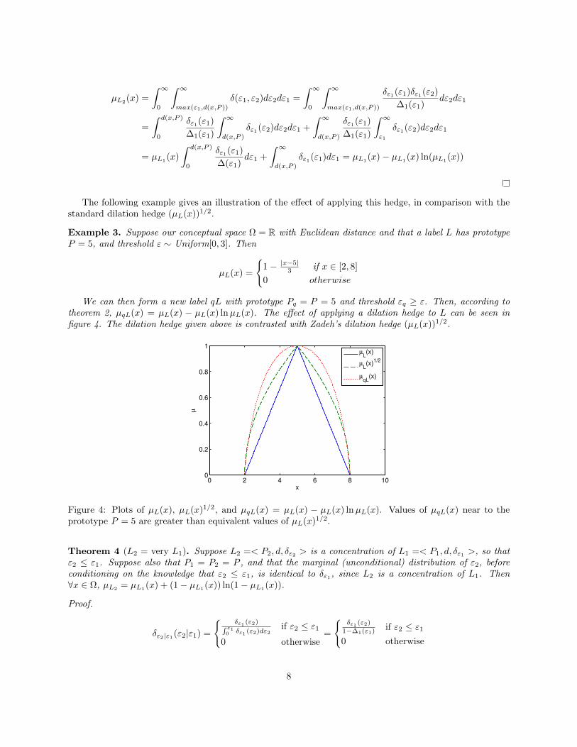
The following example gives an illustration of the effect of applying this hedge, in comparison with thestandard dilation hedge (µL(x))1/2.
Example 3. Suppose our conceptual space Ω = R with Euclidean distance and that a label L has prototypeP = 5, and threshold ε ∼ Uniform[0, 3]. Then
µL(x) =
1− |x−5|
3 if x ∈ [2, 8]
0 otherwise
We can then form a new label qL with prototype Pq = P = 5 and threshold εq ≥ ε. Then, according totheorem 2, µqL(x) = µL(x) − µL(x) lnµL(x). The effect of applying a dilation hedge to L can be seen infigure 4. The dilation hedge given above is contrasted with Zadeh’s dilation hedge (µL(x))1/2.
0 2 4 6 8 100
0.2
0.4
0.6
0.8
1
x
µ
µL(x)
µL(x)
1/2
µqL
(x)
Figure 4: Plots of µL(x), µL(x)1/2, and µqL(x) = µL(x) − µL(x) lnµL(x). Values of µqL(x) near to theprototype P = 5 are greater than equivalent values of µL(x)1/2.
Theorem 4 (L2 = very L1). Suppose L2 =< P2, d, δε2 > is a concentration of L1 =< P1, d, δε1 >, so thatε2 ≤ ε1. Suppose also that P1 = P2 = P , and that the marginal (unconditional) distribution of ε2, beforeconditioning on the knowledge that ε2 ≤ ε1, is identical to δε1 , since L2 is a concentration of L1. Then∀x ∈ Ω, µL2
= µL1(x) + (1− µL1
(x)) ln(1− µL1(x)).
Proof.
δε2|ε1(ε2|ε1) =
δε1 (ε2)∫ ε1
0 δε1 (ε2)dε2if ε2 ≤ ε1
0 otherwise=
δε1 (ε2)
1−∆1(ε1) if ε2 ≤ ε1
0 otherwise
8
and hence,
δ(ε1, ε2) = δε1(ε1)δε2|ε1(ε2|ε1) =
δε1 (ε1)δε1 (ε2)
1−∆1(ε1) if ε2 ≤ ε1
0 otherwise
So since ε2 ≤ ε1 we have that:
µL2(x) =
∫ ∞0
∫ ε1
min(ε1,d(x,P ))
δ(ε1, ε2)dε2dε1 =
∫ ∞0
∫ ε1
min(ε1,d(x,P ))
δε1(ε1)δε1(ε2)
1−∆1(ε1)dε2dε1
=
∫ ∞d(x,P )
δε1(ε1)
1−∆1(ε1)
∫ ε1
d(x,P )
δε1(ε2)dε2dε1
=
∫ ∞d(x,P )
δε1(ε1)
1−∆1(ε1)
(∫ ε1
0
δε1(ε2)dε2 −∫ d(x,P )
0
δε1(ε2)dε2
)dε1
= µL1(x)− (1− µL1
(x))
∫ ∞d(x,P )
δε1(ε1)
1−∆1(ε1)dε1 = µL1
(x) + (1− µL1(x)) ln(1− µL1
(x))
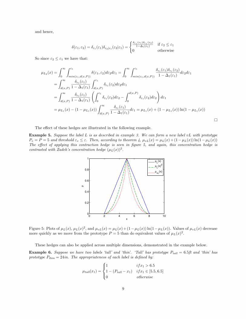
The effect of these hedges are illustrated in the following example.
Example 5. Suppose the label L is as described in example 3. We can form a new label vL with prototypePv = P = 5 and threshold εv ≤ ε. Then, according to theorem 4, µvL(x) = µL(x) + (1−µL(x)) ln(1−µL(x))The effect of applying this contraction hedge is seen in figure 5, and again, this concentration hedge iscontrasted with Zadeh’s concentration hedge (µL(x))2.
0 2 4 6 8 100
0.2
0.4
0.6
0.8
1
x
µ
µL(x)
µL(x)
2
µvL
(x)
Figure 5: Plots of µL(x), µL(x)2, and µvL(x) = µL(x)+(1−µL(x)) ln(1−µL(x)). Values of µvL(x) decreasemore quickly as we move from the prototype P = 5 than do equivalent values of µL(x)2.
These hedges can also be applied across multiple dimensions, demonstrated in the example below.
Example 6. Suppose we have two labels ‘tall’ and ‘thin’. ‘Tall’ has prototype Ptall = 6.5ft and ‘thin’ hasprototype Pthin = 24in. The appropriateness of each label is defined by:
µtall(x1) =
1 ifx1 > 6.5
1− (Ptall − x1) ifx1 ∈ [5.5, 6.5]
0 otherwise
9
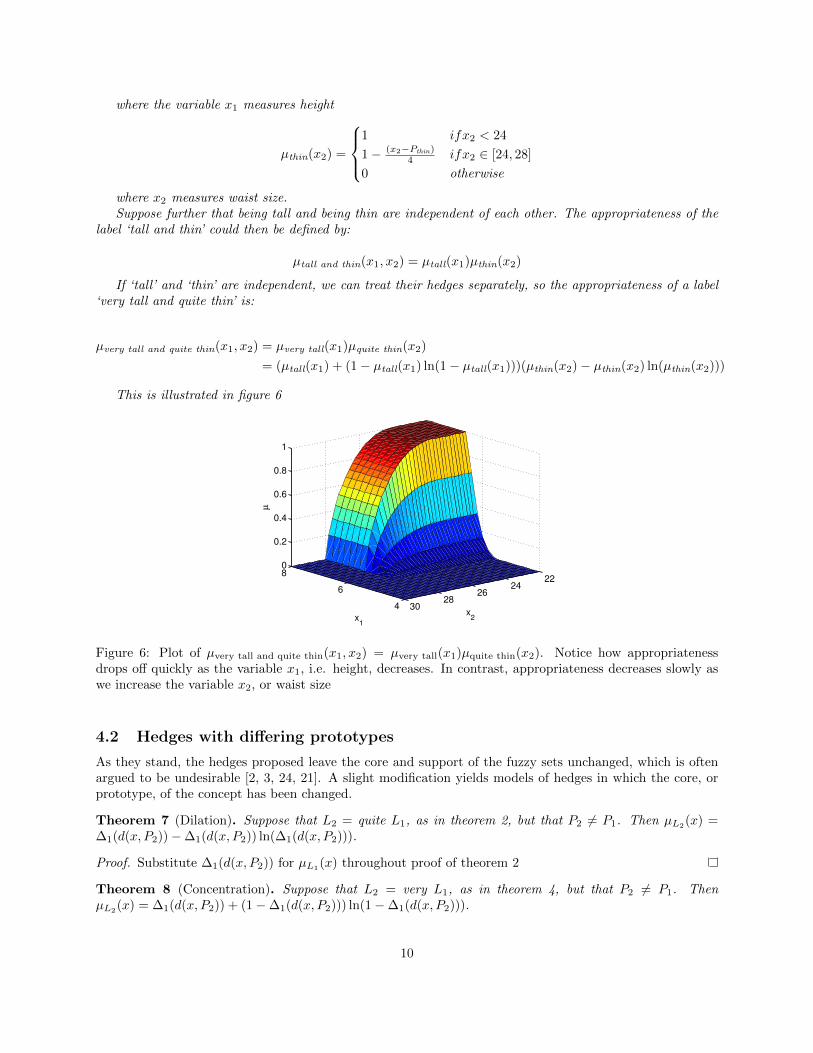
where the variable x1 measures height
µthin(x2) =
1 ifx2 < 24
1− (x2−Pthin)4 ifx2 ∈ [24, 28]
0 otherwise
where x2 measures waist size.Suppose further that being tall and being thin are independent of each other. The appropriateness of the
label ‘tall and thin’ could then be defined by:
µtall and thin(x1, x2) = µtall(x1)µthin(x2)
If ‘tall’ and ‘thin’ are independent, we can treat their hedges separately, so the appropriateness of a label‘very tall and quite thin’ is:
µvery tall and quite thin(x1, x2) = µvery tall(x1)µquite thin(x2)
= (µtall(x1) + (1− µtall(x1) ln(1− µtall(x1)))(µthin(x2)− µthin(x2) ln(µthin(x2)))
This is illustrated in figure 6
4
6
822
2426
2830
0
0.2
0.4
0.6
0.8
1
x2x
1
µ
Figure 6: Plot of µvery tall and quite thin(x1, x2) = µvery tall(x1)µquite thin(x2). Notice how appropriatenessdrops off quickly as the variable x1, i.e. height, decreases. In contrast, appropriateness decreases slowly aswe increase the variable x2, or waist size
4.2 Hedges with differing prototypes
As they stand, the hedges proposed leave the core and support of the fuzzy sets unchanged, which is oftenargued to be undesirable [2, 3, 24, 21]. A slight modification yields models of hedges in which the core, orprototype, of the concept has been changed.
Theorem 7 (Dilation). Suppose that L2 = quite L1, as in theorem 2, but that P2 6= P1. Then µL2(x) =
∆1(d(x, P2))−∆1(d(x, P2)) ln(∆1(d(x, P2))).
Proof. Substitute ∆1(d(x, P2)) for µL1(x) throughout proof of theorem 2
Theorem 8 (Concentration). Suppose that L2 = very L1, as in theorem 4, but that P2 6= P1. ThenµL2(x) = ∆1(d(x, P2)) + (1−∆1(d(x, P2))) ln(1−∆1(d(x, P2))).
10
Proof. As above.
Corollary 9. If ε2 ≥ ε1 and P2 ⊇ P1 then µL2(x) ≥ µL1
(x)−µL1(x) ln(µL1
(x)), and if ε2 ≤ ε1 and P2 ⊆ P1,then µL2
(x) ≤ µL1(x) + (1− µL1
(x)) ln(1− µL1(x)).
Proof. µL2(x) = ∆1(d(x, P2))−∆1(d(x, P2)) ln(∆1(d(x, P2))), but since P2 ⊇ P1, d(x, P2) ≤ d(x, P1) ∀x ∈ Ω,
and so ∆1(d(x, P2)) ≥ ∆1(d(x, P1)) = µL1(x) ∀x ∈ Ω. Hence, µL2(x) ≥ µL1(x)−µL1(x) ln(µL1(x)). A similarargument shows that µL2(x) ≤ µL1(x) + (1− µL1(x)) ln(1− µL1(x)).
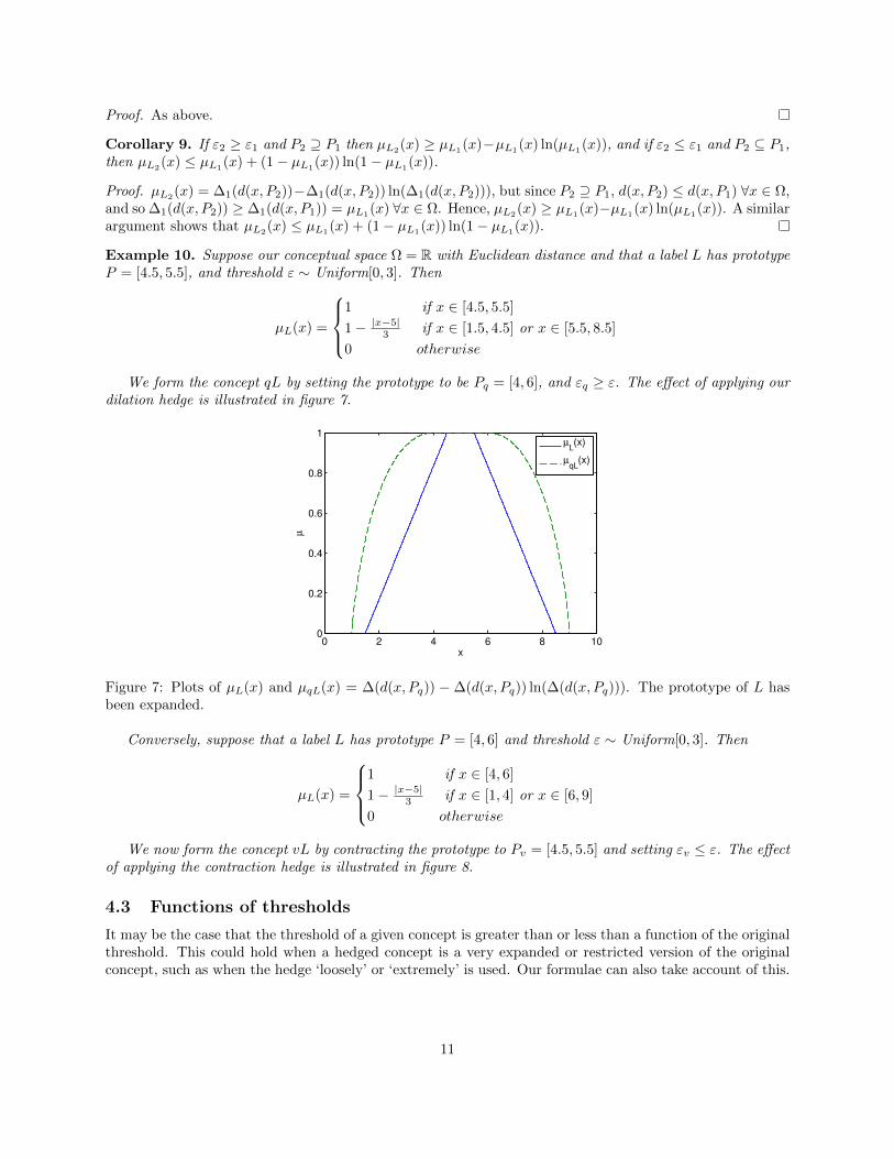
Example 10. Suppose our conceptual space Ω = R with Euclidean distance and that a label L has prototypeP = [4.5, 5.5], and threshold ε ∼ Uniform[0, 3]. Then
µL(x) =
1 if x ∈ [4.5, 5.5]
1− |x−5|3 if x ∈ [1.5, 4.5] or x ∈ [5.5, 8.5]
0 otherwise
We form the concept qL by setting the prototype to be Pq = [4, 6], and εq ≥ ε. The effect of applying ourdilation hedge is illustrated in figure 7.
0 2 4 6 8 100
0.2
0.4
0.6
0.8
1
x
µ
µL(x)
µqL
(x)
Figure 7: Plots of µL(x) and µqL(x) = ∆(d(x, Pq)) − ∆(d(x, Pq)) ln(∆(d(x, Pq))). The prototype of L hasbeen expanded.
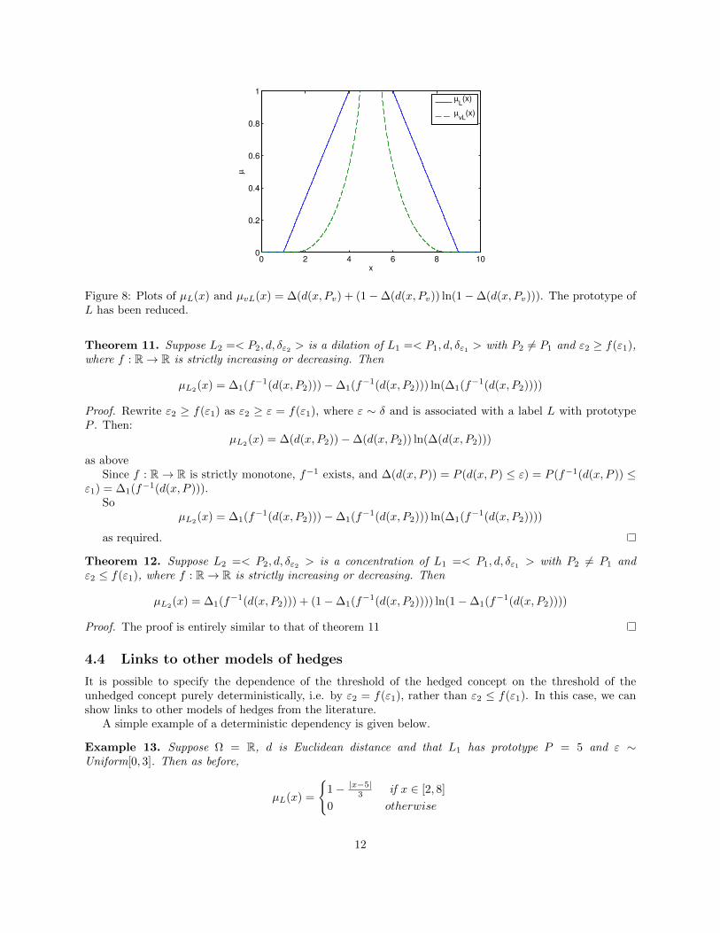
Conversely, suppose that a label L has prototype P = [4, 6] and threshold ε ∼ Uniform[0, 3]. Then
µL(x) =
1 if x ∈ [4, 6]
1− |x−5|3 if x ∈ [1, 4] or x ∈ [6, 9]
0 otherwise
We now form the concept vL by contracting the prototype to Pv = [4.5, 5.5] and setting εv ≤ ε. The effectof applying the contraction hedge is illustrated in figure 8.
4.3 Functions of thresholds
It may be the case that the threshold of a given concept is greater than or less than a function of the originalthreshold. This could hold when a hedged concept is a very expanded or restricted version of the originalconcept, such as when the hedge ‘loosely’ or ‘extremely’ is used. Our formulae can also take account of this.
11
0 2 4 6 8 100
0.2
0.4
0.6
0.8
1
x
µ
µL(x)
µvL
(x)
Figure 8: Plots of µL(x) and µvL(x) = ∆(d(x, Pv) + (1−∆(d(x, Pv)) ln(1−∆(d(x, Pv))). The prototype ofL has been reduced.
Theorem 11. Suppose L2 =< P2, d, δε2 > is a dilation of L1 =< P1, d, δε1 > with P2 6= P1 and ε2 ≥ f(ε1),where f : R→ R is strictly increasing or decreasing. Then
µL2(x) = ∆1(f−1(d(x, P2)))−∆1(f−1(d(x, P2))) ln(∆1(f−1(d(x, P2))))
Proof. Rewrite ε2 ≥ f(ε1) as ε2 ≥ ε = f(ε1), where ε ∼ δ and is associated with a label L with prototypeP . Then:
µL2(x) = ∆(d(x, P2))−∆(d(x, P2)) ln(∆(d(x, P2)))
as aboveSince f : R→ R is strictly monotone, f−1 exists, and ∆(d(x, P )) = P (d(x, P ) ≤ ε) = P (f−1(d(x, P )) ≤
ε1) = ∆1(f−1(d(x, P ))).So
µL2(x) = ∆1(f−1(d(x, P2)))−∆1(f−1(d(x, P2))) ln(∆1(f−1(d(x, P2))))
as required.
Theorem 12. Suppose L2 =< P2, d, δε2 > is a concentration of L1 =< P1, d, δε1 > with P2 6= P1 andε2 ≤ f(ε1), where f : R→ R is strictly increasing or decreasing. Then
µL2(x) = ∆1(f−1(d(x, P2))) + (1−∆1(f−1(d(x, P2)))) ln(1−∆1(f−1(d(x, P2))))
Proof. The proof is entirely similar to that of theorem 11
4.4 Links to other models of hedges
It is possible to specify the dependence of the threshold of the hedged concept on the threshold of theunhedged concept purely deterministically, i.e. by ε2 = f(ε1), rather than ε2 ≤ f(ε1). In this case, we canshow links to other models of hedges from the literature.
A simple example of a deterministic dependency is given below.
Example 13. Suppose Ω = R, d is Euclidean distance and that L1 has prototype P = 5 and ε ∼Uniform[0, 3]. Then as before,
µL(x) =
1− |x−5|
3 if x ∈ [2, 8]
0 otherwise
12
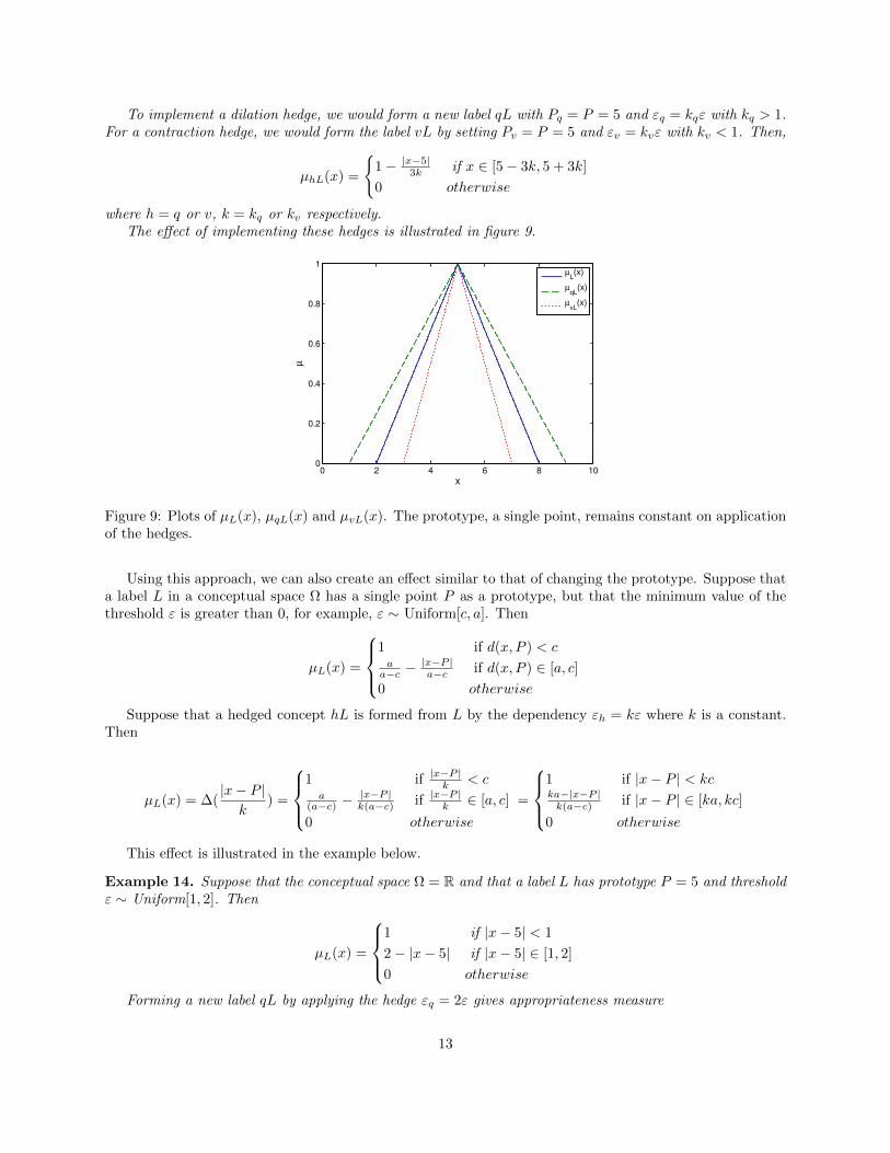
To implement a dilation hedge, we would form a new label qL with Pq = P = 5 and εq = kqε with kq > 1.For a contraction hedge, we would form the label vL by setting Pv = P = 5 and εv = kvε with kv < 1. Then,
µhL(x) =
1− |x−5|
3k if x ∈ [5− 3k, 5 + 3k]
0 otherwise
where h = q or v, k = kq or kv respectively.The effect of implementing these hedges is illustrated in figure 9.
0 2 4 6 8 100
0.2
0.4
0.6
0.8
1
x
µ
µ
L(x)
µqL
(x)
µvL
(x)
Figure 9: Plots of µL(x), µqL(x) and µvL(x). The prototype, a single point, remains constant on applicationof the hedges.
Using this approach, we can also create an effect similar to that of changing the prototype. Suppose thata label L in a conceptual space Ω has a single point P as a prototype, but that the minimum value of thethreshold ε is greater than 0, for example, ε ∼ Uniform[c, a]. Then
µL(x) =
1 if d(x, P ) < caa−c −
|x−P |a−c if d(x, P ) ∈ [a, c]
0 otherwise
Suppose that a hedged concept hL is formed from L by the dependency εh = kε where k is a constant.Then
µL(x) = ∆(|x− P |k
) =
1 if |x−P |k < ca
(a−c) −|x−P |k(a−c) if |x−P |k ∈ [a, c]
0 otherwise
=
1 if |x− P | < kcka−|x−P |k(a−c) if |x− P | ∈ [ka, kc]
0 otherwise
This effect is illustrated in the example below.
Example 14. Suppose that the conceptual space Ω = R and that a label L has prototype P = 5 and thresholdε ∼ Uniform[1, 2]. Then
µL(x) =
1 if |x− 5| < 1
2− |x− 5| if |x− 5| ∈ [1, 2]
0 otherwise
Forming a new label qL by applying the hedge εq = 2ε gives appropriateness measure
13
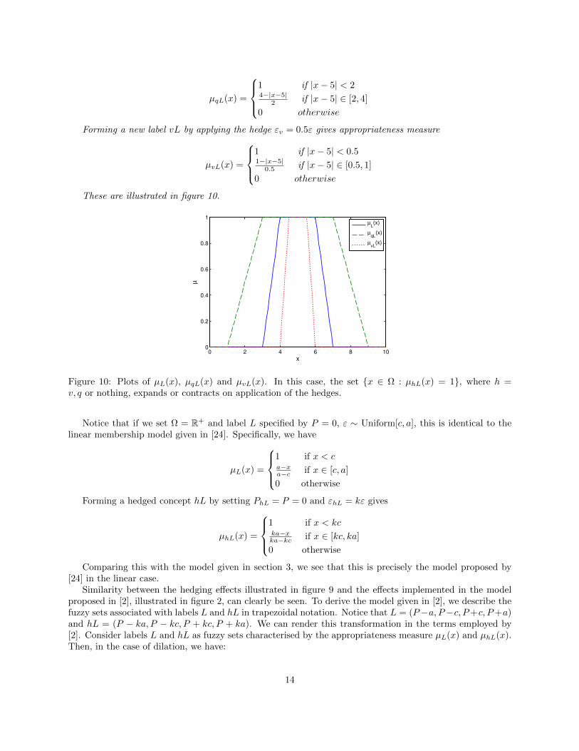
µqL(x) =
1 if |x− 5| < 24−|x−5|
2 if |x− 5| ∈ [2, 4]
0 otherwise
Forming a new label vL by applying the hedge εv = 0.5ε gives appropriateness measure
µvL(x) =
1 if |x− 5| < 0.51−|x−5|
0.5 if |x− 5| ∈ [0.5, 1]
0 otherwise
These are illustrated in figure 10.
0 2 4 6 8 100
0.2
0.4
0.6
0.8
1
x
µ
µ
L(x)
µqL
(x)
µvL
(x)
Figure 10: Plots of µL(x), µqL(x) and µvL(x). In this case, the set x ∈ Ω : µhL(x) = 1, where h =v, q or nothing, expands or contracts on application of the hedges.
Notice that if we set Ω = R+ and label L specified by P = 0, ε ∼ Uniform[c, a], this is identical to thelinear membership model given in [24]. Specifically, we have
µL(x) =
1 if x < ca−xa−c if x ∈ [c, a]
0 otherwise
Forming a hedged concept hL by setting PhL = P = 0 and εhL = kε gives
µhL(x) =
1 if x < kcka−xka−kc if x ∈ [kc, ka]
0 otherwise
Comparing this with the model given in section 3, we see that this is precisely the model proposed by[24] in the linear case.
Similarity between the hedging effects illustrated in figure 9 and the effects implemented in the modelproposed in [2], illustrated in figure 2, can clearly be seen. To derive the model given in [2], we describe thefuzzy sets associated with labels L and hL in trapezoidal notation. Notice that L = (P−a, P−c, P+c, P+a)and hL = (P − ka, P − kc, P + kc, P + ka). We can render this transformation in the terms employed by[2]. Consider labels L and hL as fuzzy sets characterised by the appropriateness measure µL(x) and µhL(x).Then, in the case of dilation, we have:
14
qL = EZ(L)(s) = supr∈ΩT (µL(s), EZ(s, r))
and for contraction,
vL = EZ(L)(s) = infr∈ΩI(µL(s), EZ(s, r))
When T is the T -norm min, I is the Godel implication and Z = (−z−α,−z, z, z+α) (with the restrictionthat c < z to ensure a well-defined set), the approach in [2] gives qL = (P −a−z−α, P −c−z, P +c+z, P +a+z+α). If we set z = (k−1)c and α = (k−1)(a−c), this is equal to qL = (P −ka, P −kc, P +kc, P +ka).
However, we also require that vL = (P − ka, P − kc, P + kc, P + ka). The approach in [2] gives vL =(P−a+z+α, P−c+z, P+c−z, P+a−z−α), and we therefore need to set z = (1−k)c and α = (1−k)(a−c)
This formulation is not as general as given in [2], however, note that it only uses one additional parameterand no additional operators, rather than the two parameters and either a T -norm or implication used by [2].
Two more key models from the literature are the powering and shifting modifiers proposed in [31].Recall that powering modifiers are of the form µhL(x) = (µL(x))k and shifting modifiers are of the formµhL(x) = (µL(x − a)). Shifting modifiers are easy to implement within our model, simply by shifting theprototype by the quantity a.
Powering modifiers can be expressed as a function of the threshold ε given a particular distribution ofthe threshold δ. Suppose Ω = R, ε ∼ U [0, c], giving
µL(x) =
1− d(x,P )
b if x ∈ [P − b, P + b]
0 otherwise
and suppose a new label hL is formed with prototype P and threshold εh = f(ε) such that µhL(x) =µL(x)k. Then µhL(x) = ∆(f−1(d(x, P ))) = (∆(d(x, P )))k, so
f−1(d(x, P )) = ∆−1((∆(d(x, P )))k) = b− b( (b− d(x, P ))k
bk) = b− (b− d(x, P ))k
bk−1
and henceεhL = f(ε) = b− (bk−1(b− ε))1/k
This expression seems surprisingly complicated, and there may be better ways of deriving the poweringhedges that are not as a function of the threshold ε.
In this section we have shown that our general model can capture some of the many approaches found inthe literature as special cases. We now go on to look at the property of compositionality that is exhibitedby a number of models.
4.5 Compositionality
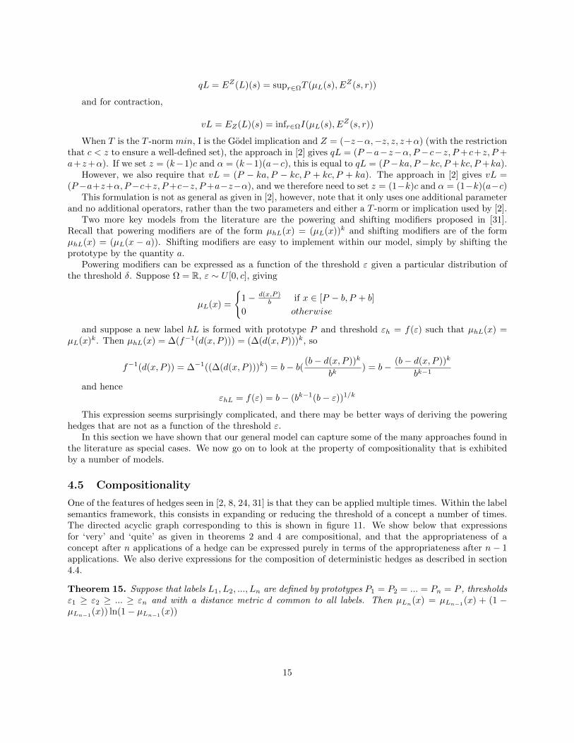
One of the features of hedges seen in [2, 8, 24, 31] is that they can be applied multiple times. Within the labelsemantics framework, this consists in expanding or reducing the threshold of a concept a number of times.The directed acyclic graph corresponding to this is shown in figure 11. We show below that expressionsfor ‘very’ and ‘quite’ as given in theorems 2 and 4 are compositional, and that the appropriateness of aconcept after n applications of a hedge can be expressed purely in terms of the appropriateness after n− 1applications. We also derive expressions for the composition of deterministic hedges as described in section4.4.
Theorem 15. Suppose that labels L1, L2, ..., Ln are defined by prototypes P1 = P2 = ... = Pn = P , thresholdsε1 ≥ ε2 ≥ ... ≥ εn and with a distance metric d common to all labels. Then µLn
(x) = µLn−1(x) + (1 −
µLn−1(x)) ln(1− µLn−1
(x))
15
ε1
ε2 ≥ ε1
ε2
ε3 ≥ ε2
ε3
εn−1
εn ≥ εn−1
εn1
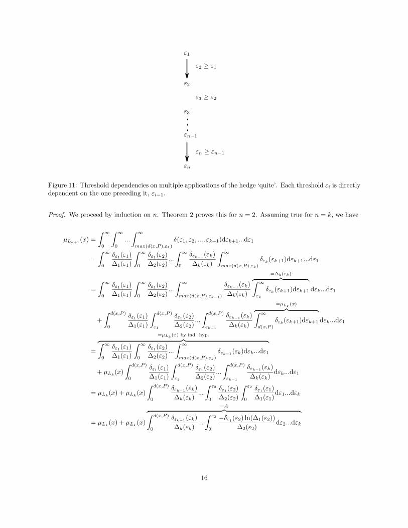
Figure 11: Threshold dependencies on multiple applications of the hedge ‘quite’. Each threshold εi is directlydependent on the one preceding it, εi−1.
Proof. We proceed by induction on n. Theorem 2 proves this for n = 2. Assuming true for n = k, we have
µLk+1(x) =
∫ ∞0
∫ ∞0
...
∫ ∞max(d(x,P ),εk)
δ(ε1, ε2, ..., εk+1)dεk+1...dε1
=
∫ ∞0
δε1(ε1)
∆1(ε1)
∫ ∞0
δε1(ε2)
∆2(ε2)...
∫ ∞0
δεk−1(εk)
∆k(εk)
∫ ∞max(d(x,P ),εk)
δεk(εk+1)dεk+1...dε1
=
∫ ∞0
δε1(ε1)
∆1(ε1)
∫ ∞0
δε1(ε2)
∆2(ε2)...
∫ ∞max(d(x,P ),εk−1)
δεk−1(εk)
∆k(εk)
=∆k(εk)︷ ︸︸ ︷∫ ∞εk
δεk(εk+1)dεk+1 dεk...dε1
+
∫ d(x,P )
0
δε1(ε1)
∆1(ε1)
∫ d(x,P )
ε1
δε1(ε2)
∆2(ε2)...
∫ d(x,P )
εk−1
δεk−1(εk)
∆k(εk)
=µLk(x)︷ ︸︸ ︷∫ ∞
d(x,P )
δεk(εk+1)dεk+1 dεk...dε1
=
=µLk(x) by ind. hyp.︷ ︸︸ ︷∫ ∞
0
δε1(ε1)
∆1(ε1)
∫ ∞0
δε1(ε2)
∆2(ε2)...
∫ ∞max(d(x,P ),εk)
δεk−1(εk)dεk...dε1
+ µLk(x)
∫ d(x,P )
0
δε1(ε1)
∆1(ε1)
∫ d(x,P )
ε1
δε1(ε2)
∆2(ε2)...
∫ d(x,P )
εk−1
δεk−1(εk)
∆k(εk)dεk...dε1
= µLk(x) + µLk
(x)
∫ d(x,P )
0
δεk−1(εk)
∆k(εk)...
∫ ε3
0
δε1(ε2)
∆2(ε2)
∫ ε2
0
δε1(ε1)
∆1(ε1)dε1...dεk
= µLk(x) + µLk
(x)
=A︷ ︸︸ ︷∫ d(x,P )
0
δεk−1(εk)
∆k(εk)...
∫ ε3
0
−δε1(ε2) ln(∆1(ε2))
∆2(ε2)dε2...dεk
16
By the inductive hypothesis, ∀i = 0...k
δεi(εi) = − d
dεi∆i(εi)
= − d
dεi(∆i−1(εi)−∆i−1(εi) ln(∆i−1(εi)))
= −δεi−1(εi) ln(∆i−1(εi))
Recursively substituting in A, we obtain
µLk+1(x) = µLk
(x) + µLk(x)
∫ d(x,P )
0
δεk−1(εk)
∆k(εk)...
∫ ε3
0
δε2(ε2)
∆2(ε2)dε2...dεk
= µLk(x) + µLk
(x)
∫ d(x,P )
0
δεk(εk)
∆k(εk)dεk
= µLk(x)− µLk
(x) ln(µLk(x))
Theorem 16. Suppose labels L1, L2, ..., Ln are defined by prototypes P1 = P2 = ... = Pn = P , thresholds ε1 ≤ε2 ≤ ... ≤ εn, and that distance metric d is common to all. Then µLn
(x) = µLn−1(x)−µLn−1
(x) ln(µLn−1(x))
Proof. Similar to proof of theorem 15.
We can also derive expressions for the composition of deterministic hedges.
Theorem 17. Suppose labels L1, L2, ..., Ln are defined by prototypes P1 = P2 = ... = Pn = P , thresholdsεn = f(εn−1), εn−1 = f(εn−2), ..., ε2 = f(ε1), where f is monotone increasing or decreasing, and thatdistance metric d is common to all. Then µLn(x) = ∆1(f−(n−1)(d(x, P )), where f−k signifies f−1 composedk times.
Proof. µL2(x) = ∆1(f−1(d(x, P )). Suppose that µLk
(x) = ∆k(d(x, P )) = ∆1(f−(k−1)(d(x, P )). Sinceεk+1 = f(εk), we have µLk+1
(x) = ∆k(f−1(d(x, P )) = ∆1(f−k(d(x, P ))).
Therefore µLn(x) = ∆1(f−(n−1)(d(x, P )) by induction.
Since labels can be composed in this way, we can model different degrees of emphasis corresponding tothe composition of multiple hedges. So, for example, we could model ‘extremely L’ as ‘very, very L’. This isillustrated in example 18.
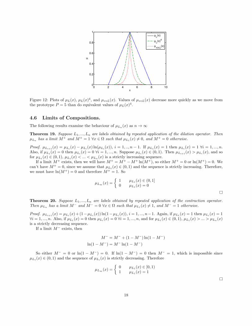
Example 18. Suppose the label L is as described in example 3, i.e. L has prototype P = 5, and thresholdε ∼ Uniform[0, 3]. We can form a new label vL with prototype Pv = P = 5 and threshold εv ≤ ε, whichhas appropriateness µvL(x) = µL(x) + (1 − µL(x)) ln(1 − µL(x)) as shown in theorem 4. We may thenform another new label vvL with prototype Pvv = Pv = 5 and threshold εvv ≤ εv with appropriatenessµvvL(x) = µvL(x) + (1 − µvL(x)) ln(1 − µvL(x)) as described in theorem 15. The effect of applying thiscontraction hedge is seen in figure 12. We have contrasted the effect of the composed hedges with (µL(x))4.
Since these hedges can be composed only an integral number of times, we cannot obtain the differences ingrade that could be achieved with using various powers in a powering modifier, e.g. µL(x)1.73. However, insection 4.3 we discuss how to tune the intensity of hedges by using dependencies on functions of thresholds.We have further shown in section 4.4 how to derive powering and shifting modifiers within our framework.It would be interesting to explore how other examples of hedges can be expressed in this framework.
We have shown that when multiple hedges of the forms seen in theorems 2 and 4 are used, µLn(x) can be
expressed purely in terms of the appropriateness of the label directly preceding it. We have not been able tofind a closed form solution for this recurrence, however, we can investigate the fixed points of the recurrenceand examine what happens to the values of µLn
(x) as n→∞. We have also shown that deterministic hedgescan be composed, and we go on to look at their behaviour in the limit of composition.
17
0 2 4 6 8 100
0.2
0.4
0.6
0.8
1
x
µ
µL(x)
µL(x)
4
µv(vL)
(x)
Figure 12: Plots of µL(x), µL(x)4, and µvvL(x). Values of µvvL(x) decrease more quickly as we move fromthe prototype P = 5 than do equivalent values of µL(x)4.
4.6 Limits of Compositions.
The following results examine the behaviour of µLn(x) as n→∞
Theorem 19. Suppose L1, ..., Ln are labels obtained by repeated application of the dilation operator. ThenµLn
has a limit M+ and M+ = 1 ∀x ∈ Ω such that µL1(x) 6= 0, and M+ = 0 otherwise.
Proof. µLi+1(x) = µLi
(x) − µLi(x) ln(µLi
(x)), i = 1, .., n − 1. If µL1(x) = 1 then µLi
(x) = 1 ∀i = 1, ..., n.Also, if µL1(x) = 0 then µLi(x) = 0 ∀i = 1, ..., n. Suppose µLi(x) ∈ (0, 1). Then µLi+1(x) > µLi(x), and sofor µL1(x) ∈ (0, 1), µL1(x) < ... < µLn(x) is a strictly increasing sequence.
If a limit M+ exists, then we will have M+ = M+ −M+ ln(M+), so either M+ = 0 or ln(M+) = 0. Wecan’t have M+ = 0, since we assume that µL1
(x) ∈ (0, 1) and the sequence is strictly increasing. Therefore,we must have ln(M+) = 0 and therefore M+ = 1. So
µL∞(x) =
1 µL1
(x) ∈ (0, 1]0 µL1(x) = 0
Theorem 20. Suppose L1, ..., Ln are labels obtained by repeated application of the contraction operator.Then µLn
has a limit M− and M− = 0 ∀x ∈ Ω such that µL1(x) 6= 1, and M− = 1 otherwise.
Proof. µLi+1(x) = µLi
(x) + (1−µLi(x)) ln(1−µLi
(x)), i = 1, ..., n−1. Again, if µL1(x) = 1 then µLi
(x) = 1∀i = 1, ..., n. Also, if µL1(x) = 0 then µLi(x) = 0 ∀i = 1, ..., n, and for µL1(x) ∈ (0, 1), µL1(x) > ... > µLn(x)is a strictly decreasing sequence.
If a limit M− exists, then
M− = M− + (1−M−) ln(1−M−)
ln(1−M−) = M− ln(1−M−)
So either M− = 0 or ln(1 −M−) = 0. If ln(1 −M−) = 0 then M− = 1, which is impossible sinceµL1
(x) ∈ (0, 1) and the sequence of µLi(x) is strictly decreasing. Therefore
µL∞(x) =
0 µL1
(x) ∈ [0, 1)1 µL1(x) = 1
18
We have shown here that in the limit, the result of applying dilation or contraction modifiers multipletimes is to create a crisp set. In the case of dilation, the crisp set includes the whole support of the fuzzy setassociated with the original label, whereas in the case of contraction, the concept reduces to include only itsprototype.
When deterministic hedges are used, i.e. ε2 = f(ε1), the behaviour of the limit depends on the behaviourof the function f and its properties in the limit as n→∞ of f−n.
Example 21. Suppose f(ε) = 0.5ε. Applying this hedge multiple times will result in µLn(x) = ∆1(2nd(x, P )).As n→∞, 2nd(x, P )→∞, except where d(x, P ) = 0. Therefore,
µL∞(x) =
0 d(x, P ) > 01 d(x, P ) = 0
On the other hand, if f(ε) = 2ε, µLn(x) = ∆1(2−nd(x, P )). As n → ∞, 2−nd(x, P ) → 0, and henceµL∞(x) = 1 ∀x ∈ Ω.
The behaviour of the hedges given in example 21 is therefore different from those in theorems 19 and20, since the concept either shrinks to a single point, in the case of contraction, or, in the case of dilation,expands to fill the entire space Ω.
5 Discussion
We have presented formulae for linguistic hedges which are both functional and semantically grounded. Themodifiers presented arise naturally from the label semantics framework, in which concepts are representedby a prototype and threshold. Our hedges have an intuitive meaning: if I think that the threshold for aconcept ‘small’ is of a certain width, then the threshold for the concept ‘very small’ will be narrower. On theother hand, the threshold for the concept ‘quite small’ will be broader. The hedges proposed are examplesof ‘type 1’ hedges, i.e. they operate equally across all dimensions of the fuzzy set associated with a concept.The first result presented is somewhat similar to a powering modifier since the core and support of the setremain the same. In [3, 22], it is argued that this property is undesirable for hedges used in fuzzy expertsystems, since if a query is returning too large a set of answers, this type of contraction hedge does notreduce this overabundance. However, although the hedges we propose do not at their simplest address theoverabundance issue, we argue that they address another problem associated with powering hedges, in thatthey have a clear semantic grounding that the powering modifiers lack.
[2, 8] also propose modifiers that are semantically grounded, using the idea of resemblance to nearbyobjects. Their formulations have the properties that the core and support of the fuzzy set are both changed,thereby addressing the issue of overabundant answers [3, 22]. In our most specific case, since the prototypeis not altered, the core and support of the fuzzy set representing the concept remain the same. However,our initial proposal can be generalised, as in section 4.2, to apply to the case where P1 6= P2. Specifying asemantically meaningful way of altering the boundaries of the prototype would answer the objection thatthe core and support of a set should change under a linguistic hedge.
The most general result (section 4.3) shows that the formula still applies when ε2 ≤ f(ε1), or ε2 ≥ f(ε1).Combined with a distribution δ such that the lower bound of the distribution is not zero, the core andsupport of the fuzzy set are modified. With the condition ε2 = f(ε1), we are able to recreate the result givenin [24] for linear membership functions, and show how the model proposed by [2] has strong similarities toour own. In this case we have introduced additional parameters, so the simplicity of the original result islost. However, the further parameters introduced are no more than those introduced by [24], and arguablyfewer than those introduced by [2], who require that a resemblance relation be specified, using two additionalparameters, and also, that a T -norm or fuzzy implication need to be specified. There are various choices ofoperator that could be used for either of these, and it is not obvious that any one is better than the others.
We have also shown that the basic case operators ‘very’ and ‘quite’ can be composed, which is notimmediately obvious from the formulae (section 4.5). Further, we show that in the limit of composition the
19
membership of any object in the fuzzy part of L, i.e. x : 0 < µL(x) < 1, increases to 1 in the case of ‘quite’or decreases to 0 in the case of ‘very’ (section 4.6). This is similar to the limit of applying the poweringmodifiers, but differs from what would happen with the modifiers proposed by [2]. In that case, the limit of‘very’ would shrink to a single point and the limit of ‘quite’ would expand to encompass the whole universe ofdiscourse. This can be modelled using the deterministic hedges described in section 4.4. Although behaviourdiffers slightly, in fact human discourse does not apply modifiers infinitely, so the difference in behaviour isarguably not important.
Our formulation has the benefit that it can be applied in more situations than simply linguistic hedges.For example, the concept ‘apple green’ has a prototype different to that of just green, and the threshold for‘apple green’ is likely to be smaller than the threshold for simply ‘green’. Our model can take account ofthis.
6 Conclusions and further work
We have presented formulae for two simple linguistic hedges, ‘very’ and ‘quite’. These formulae are functional,hence easy to compute, but also semantically grounded, in that they arise naturally from the conceptualframework of label semantics combined with prototype theory and conceptual spaces theory, and in the mostspecific case require no additional parameters. We have also shown that two other formulations [2, 8, 24],can be derived from this framework with equal or fewer parameters. We have shown that the hedges can becomposed and have described their behaviour in the limit of composition.
Further work could look at testing the utility of these hedges in particular classifiers to compare theirperformance with the classical hedges and with the hedges used by e.g. [3, 22], and also to examine a trade-offbetween accuracy and the number of parameters used. Alternatively, investigating semantically groundedways of expanding or reducing prototypes could have a similar impact.
The model could also be extended to the more complicated type 2 hedges such as ‘essentially’, or ‘tech-nically’, by treating dimensions of the conceptual space heterogeneously. This requires using some type ofweighting or necessity measure on the dimensions, work which is currently ongoing.
7 Acknowledgements
Martha Lewis gratefully acknowledges support from EPSRC Grant No. EP/E501214/1
References
[1] G. Bordogna and G. Pasi. A fuzzy linguistic approach generalizing boolean information retrieval: Amodel and its evaluation. JASIS, 44(2):70–82, 1993.
[2] P. Bosc, D. Dubois, A. HadjAli, O. Pivert, and H. Prade. Adjusting the core and/or the support of afuzzy set-a new approach to fuzzy modifiers. In Fuzzy Systems Conference, 2007. FUZZ-IEEE 2007.IEEE International, pages 1–6. IEEE, 2007.
[3] P. Bosc, A. Hadjali, and O. Pivert. Empty versus overabundant answers to flexible relational queries.Fuzzy Sets and Systems, 159(12):1450–1467, 2008.
[4] B. Bouchon-Meunier. Interpretable decisions by means of similarities and modifiers. In Fuzzy Systems,2009. FUZZ-IEEE 2009. IEEE International Conference on, pages 524–529. IEEE, 2009.
[5] N. Cat Ho and W. Wechler. Hedge algebras: an algebraic approach to structure of sets of linguistictruth values. Fuzzy Sets and Systems, 35(3):281–293, 1990.
[6] B. Cetisli. Development of an adaptive neuro-fuzzy classifier using linguistic hedges: Part 1. ExpertSystems with Applications, 37(8):6093–6101, 2010.
20
[7] A. Chatterjee and P. Siarry. Nonlinear inertia weight variation for dynamic adaptation in particle swarmoptimization. Computers & Operations Research, 33(3):859–871, 2006.
[8] M. De Cock and E.E. Kerre. A context based approach to linguistic hedges. International Journal ofApplied Mathematics and Computer Science, 12(3):371–382, 2002.
[9] L. Di Lascio, A. Gisolfi, and U. Cortes Garcia. Linguistic hedges and the generalized modus ponens.International Journal of Intelligent Systems, 14(10):981–993, 1999.
[10] D. Dubois and H. Prade. The three semantics of fuzzy sets. Fuzzy Sets and Systems, 90(2):141–150,1997.
[11] Didier Dubois and Henri Prade. Gradualness, uncertainty and bipolarity: Making sense of fuzzy sets.Fuzzy Sets and Systems, 192:3–24, 2012.
[12] M. El-Sayed and D. Pacholczyk. A qualitative reasoning with nuanced information. Logics in ArtificialIntelligence, pages 283–295, 2002.
[13] G. Frege. Sense and reference. The Philosophical Review, 57(3):209–230, 1948.
[14] P. Gardenfors. Conceptual Spaces: The Geometry of Thought. The MIT Press, 2004.
[15] N.C. Ho and H.V. Nam. An algebraic approach to linguistic hedges in Zadeh’s fuzzy logic. Fuzzy Setsand Systems, 129(2):229–254, 2002.
[16] G. Lakoff. Hedges: A study in meaning criteria and the logic of fuzzy concepts. Journal of PhilosophicalLogic, 2(4):458–508, 1973.
[17] J. Lawry. A framework for linguistic modelling. Artificial Intelligence, 155(1-2):1–39, 2004.
[18] J. Lawry. Modelling and reasoning with vague concepts, volume 12. Springer, 2006.
[19] J. Lawry and Y. Tang. Uncertainty modelling for vague concepts: A prototype theory approach.Artificial Intelligence, 173(18):1539–1558, 2009.
[20] B.D. Liu, C.Y. Chen, and J.Y. Tsao. Design of adaptive fuzzy logic controller based on linguistic-hedge concepts and genetic algorithms. Systems, Man, and Cybernetics, Part B: Cybernetics, IEEETransactions on, 31(1):32–53, 2001.
[21] J.G. Marin-Blazquez and Q. Shen. Linguistic hedges on trapezoidal fuzzy sets: A revisit. In FuzzySystems, 2001. The 10th IEEE International Conference on, volume 1, pages 412–415. IEEE, 2001.
[22] J.G. Marin-Blazquez and Q. Shen. Regaining comprehensibility of approximative fuzzy models via theuse of linguistic hedges. Studies in Fuzziness and Soft Computing, 128:25–53, 2003.
[23] J.G. Marin-Blazquez, Q. Shen, and A.F. Gomez-Skarmeta. From approximative to descriptive models.In Fuzzy Systems, 2000. FUZZ IEEE 2000. The Ninth IEEE International Conference on, volume 2,pages 829–834. IEEE, 2000.
[24] V. Novak. A horizon shifting model of linguistic hedges for approximate reasoning. In Fuzzy Systems,1996., Proceedings of the Fifth IEEE International Conference on, volume 1, pages 423–427. IEEE,1996.
[25] E. Rosch. Cognitive representations of semantic categories. Journal of Experimental Psychology: Gen-eral, 104(3):192, 1975.
[26] Glenn Shafer. A mathematical theory of evidence, volume 1. Princeton University Press Princeton,1976.
21
[27] Yongchuan Tang and Jonathan Lawry. Linguistic modelling and information coarsening based on pro-totype theory and label semantics. International Journal of Approximate Reasoning, 50(8):1177–1198,2009.
[28] Yongchuan Tang and Jonathan Lawry. A bipolar model of vague concepts based on random set andprototype theory. International Journal of Approximate Reasoning, 53(6):867–879, 2012.
[29] S. Waart van Gulik. A fuzzy logic approach to non-scalar hedges. Towards Mathematical Philosophy,pages 233–248, 2009.
[30] L.A. Zadeh. Fuzzy sets*. Information and Control, 8(3):338–353, 1965.
[31] L.A. Zadeh. A fuzzy-set-theoretic interpretation of linguistic hedges. Journal of Cybernetics, 1972.
[32] L.A. Zadeh. The concept of a linguistic variable and its application to approximate reasoning - I.Information Sciences, 8(3):199–249, 1975.
22
Top Related
Copyright © 2022 FDOKUMEN

