


Bahasa
Halaman
Hukum


Journal of Computational Physics 205 (2005) 439–457
www.elsevier.com/locate/jcp
A fast computation technique for the directnumerical simulation of rigid particulate flows
Nitin Sharma, Neelesh A. Patankar *
Department of Mechanical Engineering, Northwestern University, Evanston, IL 60208-3111, USA
Received 15 March 2004; received in revised form 18 November 2004; accepted 19 November 2004
Available online 29 December 2004
Abstract
In this paper, we present a computation technique for the direct numerical simulation of freely moving rigid bodies
in fluids. We solve three-dimensional laminar flow problems using a control volume approach. The key feature of this
approach is that the computational overhead (relative to a pure fluid solver) to solve for the motion of rigid particle is
very small. The formulation is convenient for handling irregular geometries. We present results for the sedimentation of
particles of different shapes. Convergence tests are presented to assess the order of accuracy of the numerical scheme.
Various test cases are considered and the numerical results are compared with experimental values to validate the code.
Due to the ability to perform fast computations, this method has been used for animations and its application to the
direct numerical simulation of turbulent particulate flows merits investigation. The technique is not restricted to any
constitutive model of the suspending fluid. Hence, it may potentially be used in Large Eddy Simulations (LES) or Rey-
nolds Averaged Navier–Stokes (RANS) type simulations.
� 2004 Elsevier Inc. All rights reserved.
Keywords: Direct numerical simulation; Distributed Lagrange multiplier; Rigid particulate flow; Animation; Turbulent flows
1. Introduction
Numerical simulation techniques for solid–liquid flows, which do not use any model for fluid–particle
interaction, have been developed over the past 12 years. In these methods, the fluid flow is governed bythe continuity and momentum equations, whereas the particles are governed by the equation of motion
for rigid body. The flow field around each individual particle is resolved. The hydrodynamic force between
the particles and the fluid is obtained from the solution and is not modeled by any drag law. These
0021-9991/$ - see front matter � 2004 Elsevier Inc. All rights reserved.
doi:10.1016/j.jcp.2004.11.012
* Corresponding author. Tel.: +1 847 491 3021; fax: +1 847 491 3915.
E-mail address: [email protected] (N.A. Patankar).

440 N. Sharma, N.A. Patankar / Journal of Computational Physics 205 (2005) 439–457
simulations referred to as direct numerical simulation (DNS) of solid–liquid flows, can be applied in numer-
ous settings; e.g., sedimenting and fluidized suspensions, lubricated transport, hydraulic fracturing of res-
ervoirs, slurries, understanding particle–turbulence interaction, etc.
Hu and co-workers [11–13] developed a finite-element method based on unstructured grids to simu-
late the motion of large numbers of rigid particles in two and three dimensions in Newtonian and vis-coelastic fluids. This approach is based on an arbitrary-Lagrangian–Eulerian (ALE) technique that uses
a moving mesh scheme to handle the time-dependent fluid domain. A new mesh is generated when the
old one becomes too distorted, and the flow field is projected on to the new mesh. A combined fluid–
particle weak formulation is used, where the hydrodynamic forces and torques on the particle are not
computed explicitly. Another numerical scheme based on the moving mesh technique was developed by
Johnson and Tezduyar [14]. They used a space time finite element formulation and a fully explicit
scheme in which the forces and torques on the particles were calculated explicitly to solve the equations
of rigid motion.Glowinski et al. [9] presented a distributed Lagrange-multiplier/fictitious-domain (DLM) method for the
direct numerical simulation of the motion of many rigid particles in Newtonian fluids. Their finite element
formulation permits the use of a fixed structured grid. This eliminates the need for remeshing the domain –
a necessity in the unstructured grid-based methods. Structured grids also allow the use of fast and efficient
solvers. In the DLM method, the entire fluid–particle domain is assumed to be a fluid and the flow in the
particle domain is constrained to be a rigid-body motion by using a rigidity constraint. This leads to a La-
grange multiplier field in the particle domain. The constraint of rigid body motion is represented by
u = U + x · r, where u is the velocity of the fluid at a point inside the particle domain, U and x are thetranslational and angular velocities of the particle, respectively, and r is the position vector of the point with
respect to the particle centroid. The fluid–particle motion is treated implicitly using a combined weak for-
mulation in which the mutual forces cancel.
A new DLM formulation for particulate flows was later presented by Patankar et al. [21]. In their ap-
proach, the rigid motion is imposed by constraining the deformation-rate tensor within the particle domain
to be zero. This eliminates U and x as variables from the coupled system of equations – thus enabling sim-
ulations of irregular shaped bodies without additional complexity. This formulation recognizes that the
rigidity constraint results in a stress field inside a rigid solid just as there is pressure in an incompressiblefluid. The DLM formulation of Glowinski et al. [9] and Patankar et al. [21] were implemented by using
a Marchuk–Yanenko fractional-step scheme for time discretization. A finite-element method was used.
The ALE and DLM formulations, discussed above, have been implemented for laminar flow conditions.
Although the DLM approach has been successfully used for computations with up to 1204 spheres in three
dimensions – Pan et al. [19] – further speed-up of the solution procedure is desirable. This is critical for
DNS of turbulent particulate flows or for performing simulations with thousands of particles where fast
computations are essential for the problems to be computationally feasible. With these objectives in con-
sideration, Patankar [20] presented an adapted version of his earlier DLM-based formulation – Patankaret al. [21] – for the fast computation of rigid particulate flows. The key issue addressed in the formulation
was the fast implementation of the rigidity constraint, irrespective of the type of equations used to describe
the fluid. The formulation eliminated the need for an iterative procedure to solve the rigid body projection
step thereby allowing faster computations for particulate flows.
In this paper, we have implemented the formulation developed by Patankar [20] for the case of three-
dimensional particles using a control volume approach. Our objective is to demonstrate the effectiveness
of the approach in handling three-dimensional regular and irregular shaped particles without significant
computational overhead. We report convergence tests to check the order of accuracy of the scheme. A fixedstructured grid is used in both the fluid and the particle domains. The mathematical formulation for the
problem is laid down in Section 2. The computational scheme is outlined in Section 3. The numerical imple-
mentation is outlined in Section 4. Section 5 describes the results obtained and the validation.

N. Sharma, N.A. Patankar / Journal of Computational Physics 205 (2005) 439–457 441
2. Mathematical formulation
Let X be the computational domain which includes both the fluid and the particle domain. Let P(t) be
the particle domain. Let the fluid boundary not shared with the particle be denoted by C. We will consider a
Dirichlet boundary condition on C. At times we will assume a single particle in the domain for the simplic-ity of exposition. The body force will also be assumed to be constant so that there is no net torque acting on
the particle. The governing equations for fluid motion are given by:
qf
ou
otþ u � rð Þu
� �¼ r � rþ qfg in X n P ðtÞ; ð1Þ
r � u ¼ 0 in X n PðtÞ; ð2Þ
u ¼ uCðtÞ on C; ð3Þ
u ¼ ui on oP ðtÞ; ð4aÞ
r � n ¼ t on oP ðtÞ; ð4bÞ
ujt¼0 ¼ u0ðxÞ in X n P ð0Þ; ð5Þ
where qf is the fluid density, u is the fluid velocity, g is the acceleration due to gravity, n is the outward nor-
mal on the particle surface, ui is the velocity at fluid–particle interface oP(t), r is the stress tensor and t is the
traction vector on the particle surface. The initial velocity u0 should satisfy (2). The boundary velocity, uC,
in (3) should satisfy the compatibility condition due to (2). For an incompressible fluid the divergence-free
constraint (2) gives rise to pressure in the fluid. The stress tensor is then given by:
r ¼ �pIþ s; ð6Þ
where I is the identity tensor, p is the pressure and s is the extra-stress tensor given by,
s ¼ l ruþ ruð ÞTh i
; ð7Þ
for a Newtonian fluid, where l is the viscosity of the fluid.
Particle motion can be represented in terms of translational and angular velocities using Newton�s sec-ond law. In the DLM formulation the particle is treated as a fluid that is subjected to an additional rigidity
constraint. The governing equations for the particle motion are given by [21]:
qs
ou
otþ u � rð Þu
� �¼ r � rþ qsg in P ðtÞ; ð8Þ
r � u ¼ 0 in P tð Þ; ð9Þ
D u½ � ¼ 12ruþruT� �
¼ 0 in P ðtÞ; ð10Þ
u ¼ ui on oP ðtÞ; ð11aÞ
r � n ¼ t on oP ðtÞ; ð11bÞ
ujt¼0 ¼ u0ðxÞ in Pð0Þ; ð12Þ
442 N. Sharma, N.A. Patankar / Journal of Computational Physics 205 (2005) 439–457
where qs is the particle density. The initial velocity u0 should satisfy (10). The rigidity constraint (10) en-
sures that the velocity field is divergence-free. Hence (9) is a redundant equation but is retained in order
to facilitate numerical implementation [21]. As noted earlier the incompressibility constraint (Eq. (9)),
which is a scalar constraint; gives rise to a scalar field (pressure p). Similarly the rigidity constraint
(Eq. (10)), which is a tensor constraint; gives rise to a tensor field (stress L) in the particle domain. Lis a symmetric second-order tensor. Variational analysis of the above equations shows that the pressure
p and stress L are the distributed Lagrange multipliers due to the divergence-free and rigidity constraints,
respectively [21]. L is an additional stress field required inside the particle domain to maintain the rigid-
body motion. The Lagrange multiplier stress L has six scalar variables in a three-dimensional case. This
is because Eq. (10) represents six scalar constraint equations at a point. A reformulation of Eq. (10) can
reduce the number of Lagrange multiplier variables to three. The rigidity constraint can be implemented
by imposing [21]:
r � D u½ �ð Þ ¼ 0 in P ðtÞ; ð13Þ
D u½ � � n ¼ 0 on oP ðtÞ; ð14Þ
where (13) and (14) represent three scalar constraint equations at a point. As a result L is no longer the
Lagrange multiplier itself. It remains the stress field inside the particle due to the rigidity constraint. It
can be represented in terms of a Lagrange multiplier k by [21]:
L ¼ D k½ �; ð15Þ
where k is a vector with three scalar components in a three-dimensional case. Hence, the stress inside the
particle is given by [21]:
r ¼ �pIþD½k� þ s: ð16Þ
sis zero in the particle domain due to the rigidity constraint (Eqs. (13) and (14)). Nevertheless, the term is
retained in the particle domain to facilitate the solution procedure [21].
Patankar et al. [21] solved the above fluid–particle equations using a finite element method. Patankar [20]
presented an adapted version of this formulation thus allowing for fast computation of rigid particulate
flows.
3. Computational algorithm
We present the computational algorithm based on the formulation by Patankar [20]. Assume a Newto-
nian fluid with constant viscosity l. The momentum equation applicable in the entire domain can be written
as:
ðqfð1� HÞ þ HqsÞou
otþ u � rð Þu
� �¼ �rp þ lr2uþ ðqfð1� HÞ þ HqsÞgþ f in X; ð17Þ
where f is the additional term due to the rigidity constraint in Eqs. (13) and (14) in the particle domain.
Note that f = $ Æ D[k] according to Eqs. (8) and (16). The continuity equation applicable in the entire do-
main is given by:
oðqfð1� HÞ þ HqsÞot
þr � ½ðqfð1� HÞ þ HqsÞu� ¼ 0 in X: ð18Þ

N. Sharma, N.A. Patankar / Journal of Computational Physics 205 (2005) 439–457 443
In Eqs. (17) and (18), H is a step function given by:
H ¼ 0 in X=P ðtÞ;1 in P ðtÞ:
����� ð19Þ
H moves with the particle, therefore,
DHDt
¼ 0 on oP ðtÞ; ð20Þ
where D/Dt is the material derivative. The continuity Eq. (18) combined with the definition of H (Eqs. (19)
and (20)) gives a divergence free velocity field in the entire domain. Also Eq. (17) reduces to Eq. (1) in the
fluid domain and Eq. (8) in the particle domain.
The governing equations can be solved by the following two fractional time steps [20]:
(1) Solve for u and p satisfying the following equations in the entire domain:
qf 1� Hð Þ þ Hqsð Þ u�un
Dt þ u � rð Þu� �
¼ �rp þ lr2uþ qf 1� Hð Þ þ Hqsð Þg;r � u ¼ 0:
)ð21Þ
Set unþ1 ¼ u and pnþ1 ¼ p in the fluid domain. Note that f = 0 everywhere in this step.
(2) Solve for un+1 in the particle domain by projecting u on to a rigid body motion. To do so, in the particle
domain, we have
qs
unþ1 � u
Dt
� �¼ f: ð22Þ
To solve for un+1 in step 2 one requires knowledge of f. An equation for f can be obtained by using
Eqs. (13) and (14) [20]:
r � D unþ1½ �ð Þ ¼ r � D uþ fDtqs
h i� �¼ 0;
D unþ1½ � � n ¼ D uþ fDtqs
h i� n ¼ 0:
9>=>; ð23Þ
The above equation implies that uþ ðfDt=qsÞ is a rigid body motion, but it gives no information about
what this motion should be. In fact, this rigid motion is the solution that we are looking for, because
uþ ðfDt=qsÞ ¼ unþ1 from Eq. (22).
Patankar [20] argued the rigid body motion can be obtained by imposing an additional condition
that, in the projection step, the total linear and angular momenta in the individual particle domain
should be conserved. The following procedure can be used to get the required solution.
(i) Split u as: u ¼ ur þ u0, where ur
ur ¼ Uþ x� r
MU ¼RP qsu dx and Ipx ¼
Rp r� qsu dx
); ð24Þ
where M is the mass of the particle and Ip is the moment of inertia of the particle. This computational
step is cheap since it is merely an addition (integration).
(ii) Since the linear and the angular momenta should be conserved in the projection step, set un+1 = urin the particle domain. This is the required solution. Note that f = �(qsu 0)/Dt. The velocity is cor-
rected in the particle domain (and the smeared interface). The influence of this correction is not
propagated by diffusion into the fluid in this fractional step. First, we note that there is no sharp

444 N. Sharma, N.A. Patankar / Journal of Computational Physics 205 (2005) 439–457
discontinuity of velocity in the domain; rather the velocity correction is smeared on the length
scale of the grid size. Second, the influence of the velocity correction in the particle domain does
propagate by diffusion into the fluid during the computation of the first fractional step of the next
time step. Third, the combination of the two fractional steps, i.e., the net scheme, is first-order
[9,10] also to be discussed below. Smaller time steps are preferable – as is usually recommendedfor first-order schemes.
The key advantage of the above formulation is that the projection step only involves integrations in the
particle domain with no iterations; hence, it is computationally cheap.
Some remarks on the uniqueness and similarity of this approach compared to the previous DLM formu-
lations and implementations are in order. In the above approach, U and x are not implicit variables in the
coupled system of equations. This is unlike the formulation by Glowinski et al. [9] where additional equa-
tions of motion for U and x are solved. For bodies with irregular shapes, the angular velocity equation isnon-linear. The method in this paper, where additional angular velocity equations are not required, can be
effective to simulate the motion of irregular shaped bodies without additional complexity.
The operator splitting scheme used above is like the Marchuk–Yanenko scheme used in the previous
DLM implementations [9,10,21]. Here we use the control volume discretization while previous implemen-
tations were finite element based. Eq. (24) is useful to extend the DLM approach to a control volume dis-
cretization. Incorporation of a rigid particle solver in the conventional control volume based conservative
schemes for the solution of Navier–Stokes equations, therefore, becomes straightforward.
Glowinski and co-workers [9,10] discussed different operator splitting schemes of the Marchuk–Yanenkotype, primarily depending on how the viscous term is split. One version they considered is equivalent to
keeping part of the viscous term in fractional step one (a modified Eq. (21)) and the other part in fractional
step two (a modified Eq. (22)). In this version the rigid motion projection is done coupled with the diffusion
equation in the entire domain. The computational cost of this approach, in our earlier implementations,
was consequently larger; typically taking up to 30% of the total computational time.
The other version, used widely by e.g. [9,10,21], is equivalent to keeping the entire viscous term in the
first fractional step. The rigid motion projection step is then similar to Eq. (22). As such, like the present
scheme, the rigid motion projection gives velocity correction in the particle domain and near the smearedinterface only. Thus, this aspect is also applicable to the earlier DLM implementations. As discussed above
the effect of this correction diffuses into the fluid in the next fractional step. That the net scheme is first-
order has been discussed by [9,10]. The same conclusions will apply to the formulation in this work. The
numerical results, to be presented below, confirm that our scheme is first-order.
In earlier work, the rigid body projection step similar to Eq. (22) was implemented by a variational for-
mulation (instead of Eq. (24)) that typically required 70–100 iterations (e.g. [9,10,21]). Our previous imple-
mentations of this approach usually took 5–10% computational time. In this work, the rigid motion
projection is based on Eq. (24) above, where no iterations are necessary. The typical time spent in ourimplementations using Eq. (24) is less than 1% for all the cases presented in this paper thus speeding up
the particle solver.
Dong et al. [5] compared the performance of their spectral DLM approach with the force-coupling
method (FCM) by Maxey and Patel [17]. The FCM method is based on representing the particles by
low-order force multipoles distributed over a finite volume. Dong et al. [5] reported that FCM is compu-
tationally cheaper than their DLM approach. The computational cost of their DLM approach was more in
part because of the iterations involved in the rigid motion projection that was implicitly coupled with the
diffusion term in the entire domain (they had the diffusion term in the particle projection step). In compar-ison, the cost of the fractional time stepping scheme such as that in this and in earlier works [9,10,21] is less.
This cost reduction is similar to that obtained by using e.g. a Chorin type pressure-based fractional time
stepping scheme instead of a fully implicit scheme for the solution of Navier–Stokes equations.

N. Sharma, N.A. Patankar / Journal of Computational Physics 205 (2005) 439–457 445
The method to impose the rigidity constraint presented here (without additional equations of motion for
U and x), lays a theoretical framework that is similar to the first-order Chorin [3] type schemes for the
incompressibility constraint. Even with a simple projection method represented by Eqs. (22)–(24), a sec-
ond-order scheme for the rigidity constraint can be envisaged analogous to the second-order pressure cor-
rection based fractional step schemes [16] for the incompressibility constraint. This is relegated to futurework.
The formulation above follows that presented by Patankar [20]. Independently, Glowinski and co-
workers [10,8] have presented and discussed a rigid motion projection similar to Eq. (24) but including
coupled variables U and x and a density difference dependent term. They note that it works well for neu-
trally buoyant particles (i.e., fluid and particle densities are equal); otherwise the variational formulation
based projection (instead of a scheme like in Eq. (24)) works better. There are at least two issues to con-
sider here:
1. The variational formulation, although slower in terms of computational speed, is an error minimizing
projection and thus may give better results, in general, than using Eq. (24). This issue can be minimized
by improving the order of accuracy of the current time stepping scheme by drawing analogy with the
Chorin type schemes. This is a topic of our continuing work.
2. We solve Eq. (21) by accounting for the density variation. That leads to a projection step (Eq. (22)) that
does not involve a term dependent on the density difference. Unlike our present scheme, a formulation
with a density difference dependent term in the rigid projection equation is discussed by Patankar [20],
which has similarities to a scheme independently proposed by Glowinski et al. [10]. The density differencedependent term, which includes inertia and gravity effect, is an additional source term in the rigid pro-
jection step (see Patankar [20]). Thus, there is an additional velocity correction in the particle domain.
The associated error is minimized in a variational formulation based method. This may improve its per-
formance relative to Eq. (24). For neutrally buoyant particles there is no density difference dependent
term in rigid projection, thus the advantage of the variational formulation based projection is reduced.
This is consistent with the observation of Glowinski et al. [10]. In our case, even if the fluid and particle
densities are not the same, this is not an issue since we do not have a density difference dependent term in
Eq. (22).
The numerical implementation will be presented in the following section.
4. Numerical implementation
The various steps involved in the numerical implementation of the algorithm above are described below.
We use a control volume method based on staggered grids [22]. Main control volumes (Fig. 1(a)) are usedfor defining pressure and staggered control volumes are used for defining x (Fig. 1(b)), y (Fig. 1(c)) and z-
direction velocities, respectively. The arrows in Fig. 1 indicate the locations where the respective velocity
components are defined.
4.1. Computation of volume fraction u
The first step is to calculate the volume fraction u occupied by the solid particle in each of the main con-
trol volumes. This is accomplished by the following steps:
� The largest cuboid that can enclose the solid particle is identified. The main control volumes forming this
cuboid are marked.

o o
o
y
x
(a) (b) (c)
Fig. 1. The marked regions are: (a) main control volume (b) staggered control volume for u (x-direction) velocities and (c) staggered
control volume for v (y-direction) velocities. The arrows indicate the locations where the respective velocity components are defined.
446 N. Sharma, N.A. Patankar / Journal of Computational Physics 205 (2005) 439–457
� Each of the marked main control volumes is subdivided into N number of finer volumes. The centre co-
ordinates of each of these finer volumes in a given main control volume are checked to see if they lie
within the boundaries of the solid particle. To illustrate this step further consider a disc; with radius r
and thickness h as shown in Fig. 2. Let rc be the position vector of the centre of the disc (xc, yc, zc),
rfv be the position vector of the centre of the finer volume (xfv, yfv, zfv) and n be the unit vector along
the central axis of the disc.
To mark the finer volume as either being within the solid boundary or not we check for the following
conditions.(i) We define length, Lp as
Lp ¼ rfv � rc� �
� n�� ��; ð25Þ
where | | denotes the magnitude of the vector. Lp must satisfy the following condition if rfv is inside the
disc
Lp 6 r: ð26Þ
rc rfv
x
y
rfv-rc
n
h (xc, yc, zc)(xfv, yfv, zfv)
r (xc, yc, zc)
Main control volume
(xfv, yfv, zfv)
Finervolume
(a) (b)
Fig. 2. (a) Side view and (b) top view of a disc along with typical main and fine control volumes.

N. Sharma, N.A. Patankar / Journal of Computational Physics 205 (2005) 439–457 447
(ii) (xfv, yfv, zfv) should also lie within the planes bounding the disc,
abs rfv � rc� �
� n�
6h2: ð27Þ
If Eqs. (26) and (27) are satisfied; we mark the point to belong inside the disc. This scheme was used, e.g.,
in the calculations of the sedimentation of a disc, presented in Section 5. Similarly, other shapes were alsoconsidered.
� Out of the N fine control volumes in a given main control volume, let Ns have their centers inside the
particle domain. The volume fraction u for this main control volume is given by
u ¼ Ns
N: ð28Þ
In the above scheme, u is calculated by a discretization of the main control volume. The accuracy of the
approach is good when the fine control volume has an edge length that is small compared to the particle
size. We have used the fine control volume edge length that is 1/10 of the edge length of the main control
volume. The error relative to the exact value is less than 0.1%.
4.2. Solution of the fluid equations
As outlined in the section on computational algorithm, in the first fractional step, the fluid equations are
solved in the entire domain. The fluid equation (21) are discretized using the control volume approach:
ZVqnþ1u� qnun
Dtþr � ðqnþ1uuÞ � lr2uþrpnþ1 � qnþ1g
�dV ¼ 0; ð29Þ
ZV
qnþ1 � qn
Dtþr � ðqnþ1uÞ
�dV ¼ 0; ð30Þ
where V represents any control volume over which the integration is performed, and
q ¼ qfð1� uÞ þ qsu: ð31Þ
u is projected, in the next step, on to a rigid body motion in the particle domain. The volume fraction utakes values between 0 and 1 for control volumes partially occupied by the solid particle, 1 for control vol-
umes fully occupied by the solid particle and zero otherwise. The volume fraction u is the same as function
H defined earlier with the difference that it is smeared on the edge of the particle due to discretization.
The continuity Eq. (30) appears to be for a compressible fluid. This is because of smearing of u at the
particle boundary. Beyond the particle boundary region, the velocity field is indeed divergence free.
The SIMPLER (semi-implicit method for pressure linked equations – revised) algorithm by Patankar[22] is used for the solution of the discretized Eqs. (29) and (30). A fully implicit scheme is used for time
discretization and a power law scheme is used for discretizing the flux term (convection-diffusion fluxes).
A simple block correction based multigrid solver proposed by Sathyamurthy and Patankar [23] is used
to solve the resulting linear equations.
4.3. Rigid body projection of the velocity field in the particle domain
The next step is to project the velocity field u in the particle domain onto a rigid body motion ur. This isaccomplished by numerically solving for the translational velocity U and angular velocity xof the solid par-
ticle by using conservation of the angular and linear momentum given by Eqs. (32) and (33):
448 N. Sharma, N.A. Patankar / Journal of Computational Physics 205 (2005) 439–457
MU ¼ZPuqsu dx; ð32Þ
Ipx ¼ZPur� qsu dx: ð33Þ
For the case of a sphere, the moment of inertia Ip, is a diagonal matrix with all the diagonal entries equal
irrespective of the orientation of the main co-ordinate axes. For other geometries like a disc or a box it isnot a diagonal matrix unless the principal axes of the object coincide with the main co-ordinate system. Ipcan be evaluated by computing the following integral over the particle domain.
Ip ¼ZPqs r � rð ÞI� r� r½ � dx: ð34Þ
The velocity field ur in the particle domain is given by,
ur ¼ Uþ x� r: ð35Þ
Linear interpolation of velocity is done to numerically calculate U and x according to Eqs. (32) and (33).
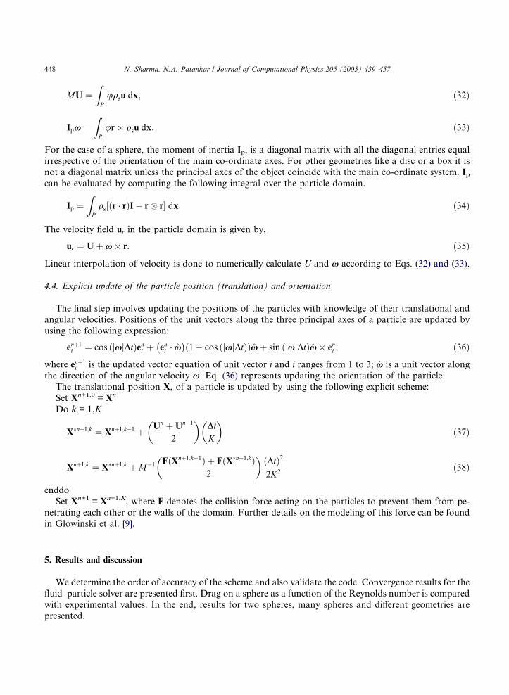
4.4. Explicit update of the particle position (translation) and orientation
The final step involves updating the positions of the particles with knowledge of their translational andangular velocities. Positions of the unit vectors along the three principal axes of a particle are updated by
using the following expression:
enþ1i ¼ cos xj jDtð Þeni þ eni � x
� �1� cos xj jDtð Þð Þxþ sin xj jDtð Þx� eni ; ð36Þ
where enþ1i is the updated vector equation of unit vector i and i ranges from 1 to 3; x is a unit vector along
the direction of the angular velocity x. Eq. (36) represents updating the orientation of the particle.The translational position X, of a particle is updated by using the following explicit scheme:
Set Xn+1,0 = Xn
Do k = 1,K
X�nþ1;k ¼ Xnþ1;k�1 þ Un þUn�1
2
� �DtK
� �ð37Þ
Xnþ1;k ¼ X�nþ1;k þM�1 FðXnþ1;k�1Þ þ FðX�nþ1;kÞ2
� �ðDtÞ2
2K2ð38Þ
enddo
Set Xn+1 = Xn+1,K, where F denotes the collision force acting on the particles to prevent them from pe-
netrating each other or the walls of the domain. Further details on the modeling of this force can be foundin Glowinski et al. [9].
5. Results and discussion
We determine the order of accuracy of the scheme and also validate the code. Convergence results for the
fluid–particle solver are presented first. Drag on a sphere as a function of the Reynolds number is compared
with experimental values. In the end, results for two spheres, many spheres and different geometries arepresented.

N. Sharma, N.A. Patankar / Journal of Computational Physics 205 (2005) 439–457 449
5.1. Convergence results
In this sub-section we discuss results of the convergence test for the fluid and the fluid–particle solvers.
Convergence test for the fluid solver only (i.e., without the particle projection step) was done to verify that,
as expected, it is second-order with respect to the grid size for the problem with uniform fluid properties.We considered a Poiseuille flow inside a channel of square cross-section. The fluid solver was found to be
second-order after plotting the error as a function of the grid size on a log-log plot.
Next we test the fluid–particle solver. We consider a single solid sphere of density 3 kg/m3 and diameter
0.625 m falling under gravity in a rectangular channel of cross-section 2 m · 2 m and height 8 m. The fluid
viscosity is 0.05 kg/ s and the density is 2 kg/m3. Simulations were carried out for increasing grid refinement.
A blocking ratio of 0.3125 was considered. The blocking ratio a is defined as the ratio of sphere diameter d
to edge length L of the cross-section of the channel
a ¼ d=L: ð39Þ
The terminal velocity of the sphere averaged over several time steps was compared with the results obtainedexperimentally by McNown et al. [18]. Fig. 3 shows a plot of the terminal velocity obtained from numerical
simulations as a function of the grid size. In the limit of the grid size going to zero the value obtained (y
intercept value) is in reasonably good agreement with the experimental values (approximately 6% differ-
ence). Ideally this difference should be zero if the experimental error is zero. It should be noted that the
experimental value was read from a graph. The errors associated with the data, which were not given byMcNown et al. [18], could account for the 6% difference in the zero grid size limit.
Brown and Lawler [1] systematically analyzed the sphere drag data available to date. They proposed cor-
relations for the drag coefficient and the terminal velocity of a sphere falling in an infinite medium by sys-
tematically eliminating the wall effects in the experimental data. The wall effect is best represented in the
graph by Fidleris and Whitmore [6]. Using the correlations by Brown and Lawler [1] and the wall effect
given by Fidleris and Whitmore [6] we calculated the terminal velocity of the sphere, for the case considered
here, to be 1.2722 m/s compared to the zero grid size limit value of 1.2453 m/s in Fig. 3. The discrepancy
according to this comparison is 2%. A discrepancy of 5% with the experimental data is reported even withthe best available curve fits [1].
y = 2.5474x - 1.2453
R2 = 0.9998
-1.16
-1.15
-1.14
-1.13
-1.12
-1.11
-1.1
-1.09
-1.08
-1.07
0.03 0.035 0.04 0.045 0.05 0.055 0.06 0.065 0.07
Grid size (m)
Ter
min
al v
eloc
ity (
m/s
)
Fig. 3. Plot of the terminal velocity as a function of grid size for a = 0.3125.

450 N. Sharma, N.A. Patankar / Journal of Computational Physics 205 (2005) 439–457
The inset equation for the trend line shows that the algorithm is first-order with respect to the grid size.
The fluid solver was second-order for a constant property fluid. The reduction in the accuracy can be attrib-
uted to the simple linear interpolation used, in the rigid body projection step and, to account for the dif-
ferent material property (density) in the particle domain. It can also be caused by the explicit update of the
particle positions. The explicit scheme is first-order with respect to time stepping. This directly influencesthe calculation of the convection term in the momentum equation, thus affecting the spatial accuracy.
Being first-order is not a limitation of the approach and as discussed before a second-order scheme for
the rigidity constraint can be envisaged analogous to the second-order pressure correction based fractional
step schemes for the incompressibility constraint.
The accuracy of the solution in the vicinity of the particle boundary depends on the interpolation
schemes used in the integrations in Eqs. (32) and (33). A better interpolation scheme, compared to the cur-
rently used linear interpolation, could improve the accuracy of the method.
The time spent in the computation of the volume fraction and the particle projection step is less than1% of the total time spent for all the computations presented here. Thus, we see that this approach has
very little computational overhead for the calculation of particle motion compared to the fluid solver.
This is true even when the number of particles are increased as in the case of results presented in Section
5.3.
To further validate the code, different test cases were considered. The first test case involved checking the
drag on a sphere of radius 0.2 m settling at finite Reynolds numbers. A blocking ratio of 0.2 was taken. The
drag coefficient CD and the Reynolds number Re of the flow are given by,
Table
Comp
Reyno
41.8
40.4
33
32.4
11.7
CD ¼ 8F D
qfU2pd2
; ð40Þ
Re ¼ qfUdl
; ð41Þ
where U is the terminal velocity of the sphere, and the drag on the sphere, FD, is given by
F D ¼ p6d3 qs � qfð Þg: ð42Þ
The Reynolds number was varied by changing the fluid and particle densities, and the fluid viscosity. The
domain size is the same as that used in the previous case. Table 1 gives the values of drag coefficient CD as afunction of the Reynolds number Re obtained numerically and experimentally [18] for a blocking ratio of
0.2 and a grid size of 0.05.
For a blocking ratio of 0.3125 and the same grid size as that used in forming Table 1, the percentage
difference is approximately 11%. As stated above, in the limit of the grid size approaching zero, for a block-
ing ratio of 0.3125, the difference reduces to 6%. Similarly, the difference in Table 1 will decrease as the grid
size decreases further.
1
arison of the numerical and experimental [18] values of drag coefficients for varying Reynolds number at a blocking ratio of 0.2
lds number Drag coefficient Difference (%)
Numerical Experimental [18]
2.29 2 13.01
2.28 2 12.26
2.56 2.12 14.61
2.49 2.12 12.27
4.9 4.27 12.97
N. Sharma, N.A. Patankar / Journal of Computational Physics 205 (2005) 439–457 451
We have further verified our rigid body projection scheme presented here but applied to steady state
Stokes flow around a periodic array of spheres. The computed drag coefficient was found to be in good
agreement with the analytical values within 2–5%. This is published elsewhere [24,25].
Mordant and Pinton [26] presented experimental data for the sedimentation of spheres. Their Reynolds
numbers were typically large and the blockage ratio was very small (�0.005), i.e., the wall effects were neg-ligible. In fact their data agree with those compiled by Brown and Lawler [1]. Our minimum blockage ratio
was 0.2 below which it is computationally expensive for our current capability. However, Mordant and
0
0.2
0.4
0.6
0.8
1
1.2
0 0.5 1 1.5 2 2.5 3
t/τ95
V/U
Mordant & Pinton
Simulation
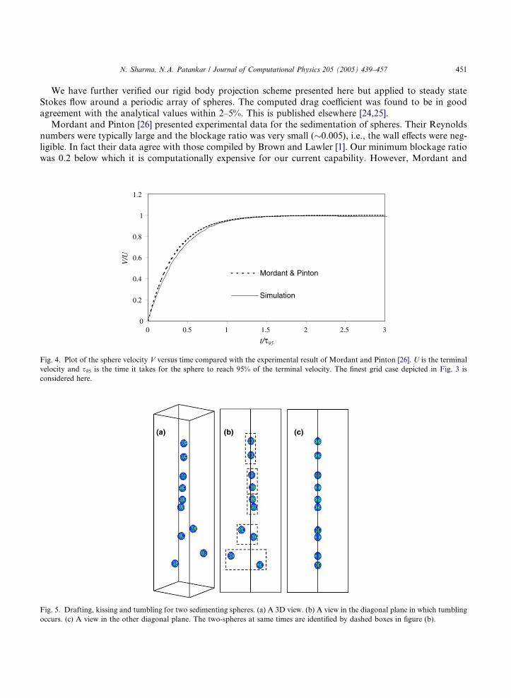
Fig. 4. Plot of the sphere velocity V versus time compared with the experimental result of Mordant and Pinton [26]. U is the terminal
velocity and s95 is the time it takes for the sphere to reach 95% of the terminal velocity. The finest grid case depicted in Fig. 3 is
considered here.
Fig. 5. Drafting, kissing and tumbling for two sedimenting spheres. (a) A 3D view. (b) A view in the diagonal plane in which tumbling
occurs. (c) A view in the other diagonal plane. The two-spheres at same times are identified by dashed boxes in figure (b).

452 N. Sharma, N.A. Patankar / Journal of Computational Physics 205 (2005) 439–457
Pinton [26] data can be used to verify the transient behavior of sedimenting particles similar to the test done
by Dong et al. [5] for their spectral DLM code. This comparison is shown in Fig. 4. The agreement is found
to be good. Similar agreement was seen for all the sphere cases considered here.
In the remaining sections we will consider test cases to verify that the numerical scheme captures the key
qualitative aspects of some important flows.
5.2. Drafting, kissing and tumbling for two interacting spheres sedimenting in a Newtonian fluid
The case of two spheres falling in a Newtonian fluid was considered to further validate our method. An
important mechanism in this case is known as ‘‘drafting, kissing and tumbling’’: see Fortes et al. [7]. The
leading particle creates a wake of low pressure. The trailing particle is caught in its wake. It experiences
lower drag hence falls faster than the leading one. This phenomenon is called drafting. The increased speed
of the trailing particle impels a kissing contact with the leading particle. In kissing contact the two spheres
0
0.5
1
1.5
2
2.5
3
3.5
4
Ver
tical
pos
ition
(cm
)
Glowinski et al.,2001
Our simulations
-9
-8
-7
-6
-5
-4
-3
-2
-1
0
0 0.1 0.2 0.3 0.4 0.5 0.6 0.7Time (s)
0 0.1 0.2 0.3 0.4 0.5 0.6 0.7Time (s)
Ver
tica
l vel
ocit
y (c
m/s
)
Glowinski et al., 2001
Our simulations
(a)
(b)
Fig. 6. Plots for drafting, kissing and tumbling of spheres shown in Fig. 5. Comparison of: (a) the vertical positions of the spheres and
(b) the vertical velocities of the spheres with the results by Glowinski et al. [10].

N. Sharma, N.A. Patankar / Journal of Computational Physics 205 (2005) 439–457 453
form a long body with the line of center along the stream. This state is unstable in a Newtonian fluid and as
a result the particles tumble under the influence of a couple which tries to bring them in broadside stable
state. The tumbling particles in a Newtonian fluid induce anisotropy of suspended particles since on the
average the line of centers between particles must be across the stream.
Fig. 5 shows numerical results for the case of two spheres of density 1.14 g/cm3 and radius 0.083 cm fall-ing under gravity in a rectangular channel of cross section 1 cm · 1 cm and height 4 cm. A Newtonian fluid
of viscosity 0.01 g/cm s and density 1 g/cm3 is considered. The spheres were initially located at heights of 3.5
and 3.16 cm, respectively. This case is chosen to be identical to that presented by Glowinski et al. [10]. As
can be seen from the snap shots taken at times 0.05, 0.25, 0.35, 0.5 and 0.7 s the spheres exhibit the known
drafting, kissing and tumbling behavior. Tumbling occurs in one of the diagonal planes and the two spheres
move on either side of the centerline.
Figs. 6(a) and (b) show comparison, of the vertical positions and velocities of the spheres, with the
results of Glowinski et al. [10]. As expected the comparison is found to be good up to the kissing ofthe particles. It is known that the tumbling phenomenon is the realization of an instability. Different
modes of tumbling have been reported in literature e.g. tumbling in a diagonal plane [10] or a plane par-
allel to the channel walls [4]. Particle positions with respect to the centerline after tumbling can also be
different e.g. both particles on same side of the centerline [10] or both particles on opposite side of the
centerline [4]. Thus the details of the motion after kissing depend on how the tumbling occurs; an exact
agreement in this part is not expected. The mode of tumbling depends on how the instability grows in a
particular numerical implementation. This is clear from Figs. 6(a) and (b), where our results are different
from those by Glowinski et al. [10] in the tumbling and later phases. In both cases the tumbling occurs inthe diagonal plane, however, in our case the particles move on either side of the centerline while in case
of Glowinski et al. [10] they move to the same side of the centerline. This leads to different velocity and
position plots. In the position plot we see that the lagging particle remains lagging in our case while in
case of Glowinski et al. [10] the lagging particle moves ahead (hence the cross-over in dotted lines in Fig.
6(b)).
1.2
0.4
1.2
2
0.60.4
2
Fig. 7. Top view of the arrangement of the spheres in a single layer (all units are in meters).

454 N. Sharma, N.A. Patankar / Journal of Computational Physics 205 (2005) 439–457
Our simulations are for a mesh size of 1/40 cm and a time step of 0.005 s. A collision scheme similar to
that by Glowinski et al. [9,10] was used to prevent particles from overlapping. The parameters in the col-
lision model per the definitions in Glowinski et al. [9] are e = 3 · 10�5 and q = 0.05 (note that q is not the
density) in CGS units. The mesh and time step of Glowinski et al. [10] is more refined; correspondingly they
are able to choose parameters such that the collision is more like those of hard spheres unlike ours.
5.3. Sedimentation of many spheres
Simulation was done for the sedimentation of 10 spheres to show that the scheme is capable of handling
many spheres. Fig. 7 shows a top view of the arrangement of the spheres in one layer.
Two such layers at heights 7.65 m and 7.05 m were considered. Spheres of density 5 kg/m3 and radius
0.2 m fall under gravity in a rectangular channel of cross section 2 m · 2 m and height 8 m. A Newtonian
fluid of viscosity 0.05 kg/m s and density 3 kg/m3 is considered.Fig. 8(a) shows a three dimensional view of the sedimenting spheres and Fig. 8(b) shows the side views.
Snapshots were taken at times 0.25, 2.25, 4.25 and 6.25 s.
Fig. 8. (a) Three dimensional view of sedimenting spheres. (b) Side view of the sedimenting spheres.
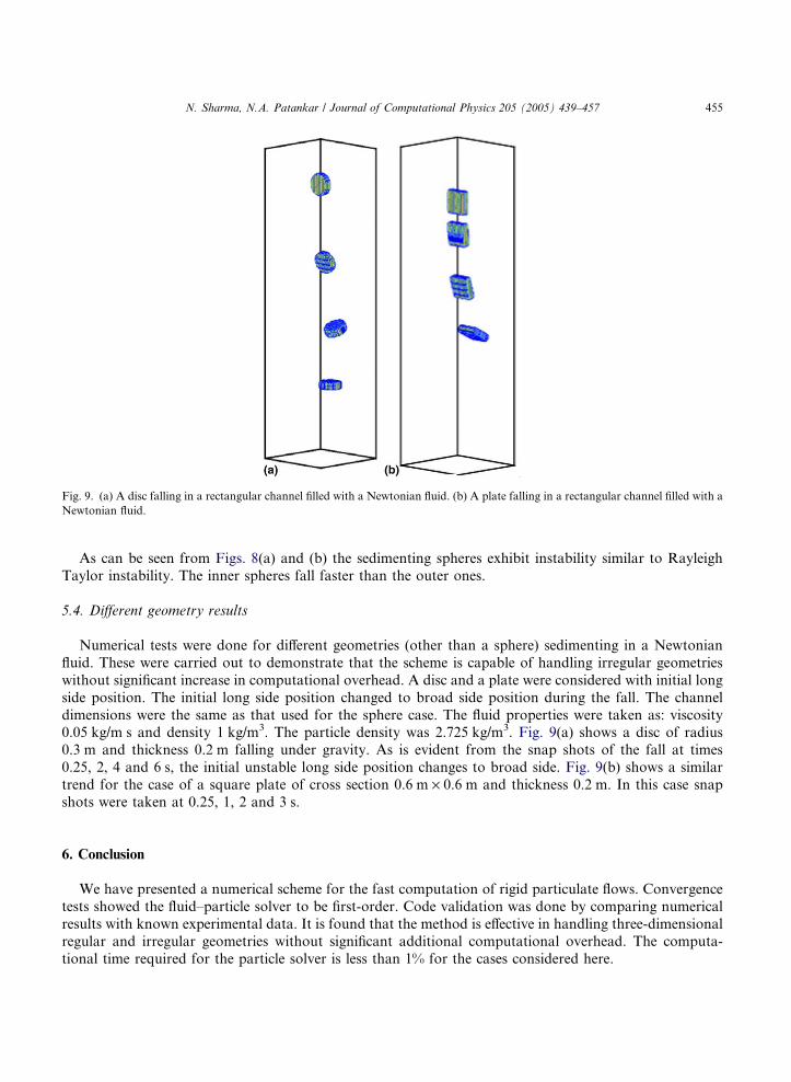
Fig. 9. (a) A disc falling in a rectangular channel filled with a Newtonian fluid. (b) A plate falling in a rectangular channel filled with a
Newtonian fluid.
N. Sharma, N.A. Patankar / Journal of Computational Physics 205 (2005) 439–457 455
As can be seen from Figs. 8(a) and (b) the sedimenting spheres exhibit instability similar to Rayleigh
Taylor instability. The inner spheres fall faster than the outer ones.
5.4. Different geometry results
Numerical tests were done for different geometries (other than a sphere) sedimenting in a Newtonian
fluid. These were carried out to demonstrate that the scheme is capable of handling irregular geometries
without significant increase in computational overhead. A disc and a plate were considered with initial long
side position. The initial long side position changed to broad side position during the fall. The channel
dimensions were the same as that used for the sphere case. The fluid properties were taken as: viscosity0.05 kg/m s and density 1 kg/m3. The particle density was 2.725 kg/m3. Fig. 9(a) shows a disc of radius
0.3 m and thickness 0.2 m falling under gravity. As is evident from the snap shots of the fall at times
0.25, 2, 4 and 6 s, the initial unstable long side position changes to broad side. Fig. 9(b) shows a similar
trend for the case of a square plate of cross section 0.6 m · 0.6 m and thickness 0.2 m. In this case snap
shots were taken at 0.25, 1, 2 and 3 s.
6. Conclusion
We have presented a numerical scheme for the fast computation of rigid particulate flows. Convergence
tests showed the fluid–particle solver to be first-order. Code validation was done by comparing numerical
results with known experimental data. It is found that the method is effective in handling three-dimensional
regular and irregular geometries without significant additional computational overhead. The computa-
tional time required for the particle solver is less than 1% for the cases considered here.
456 N. Sharma, N.A. Patankar / Journal of Computational Physics 205 (2005) 439–457
The proposed numerical method does not include additional equations of motion for the particle trans-
lational and angular velocities. The application to irregular shaped bodies is straightforward. The capabil-
ity for fast computation is rooted in a simple projection scheme for rigid motion (Eq. (24)). At the same
time the formulation lays a theoretical framework analogous to the Chorin [3] type fractional step schemes
for incompressible fluids. Improvement in the performance of this method is possible by developing higherorder time stepping schemes analogous to the pressure correction based fractional step schemes [16] for the
incompressibility constraint.
The ability to perform fast computations is suitable for the application of this method to turbulent par-
ticulate flows. This should be investigated especially in light of a method reported by Kajishima et al. [15]. It
is evident [20], that the method presented here, may be used to improve upon the earlier method by Kaji-
shima et al. [15]. Since the technique is not restricted to any constitutive model of the suspending fluid it
may also be used in large eddy simulations (LES) or Reynolds averaged Navier–Stokes (RANS) type
simulations.The ease of handling irregular shaped bodies and the fast computation capability has enabled the appli-
cation of this technique in animation. Carlson et al. [2] have applied this technique to animate the interplay
between rigid bodies and fluid. They call it the rigid fluid method. They have reported several animations of
objects of different shapes.
Acknowledgments
This work was supported by National Science Foundation under the Grant CTS-0134546. N.A.P.
acknowledges Prof. Parviz Moin for helpful discussion.
References
[1] P.P. Brown, D.F. Lawler, Sphere drag and settling velocity revisited, J. Environ. Engng. 129 (2003) 222–231.
[2] M. Carlson, P.J. Mucha, G. Turk, Rigid fluid: animating the interplay between rigid bodies and fluid, ACM Transactions on
Graphics 23 (2004) 377–384.
[3] A.J. Chorin, Numerical solution of the Navier–Stokes equations, Math. Comput. 22 (1968) 745–762.
[4] G.C. Diaz, P.D. Minev, K. Nandakumar, Fictitious domain/finite element method for particulate flows, J. Comput. Phys. 192 (1)
(2003) 105–123.
[5] S. Dong, D. Liu, M.R. Maxey, G.E. Karniadakis, Spectral distributed Lagrange multiplier method: algorithm and benchmark
tests, J. Comp. Phys. 195 (2004) 695–717.
[6] V. Fidleris, R.L. Whitmore, Experimental determination of the wall effect for spheres falling axially in cylindrical vessels, Br. J.
Appl. Phys. 12 (1961) 490–494.
[7] A. Fortes, D.D. Joseph, T.S. Lundgren, Nonlinear mechanics of fluidization of beds of spherical particles, J. Fluid Mech. 177
(1987) 467–483.
[8] R. Glowinski, Finite element methods for incompressible viscous flow, in: P.G. Ciarlet, J.L. Lions (Eds.), Handbook of
Numerical Analysis, vol. IX, North-Holland, Amsterdam, 2003, pp. 3–1176.
[9] R. Glowinski, T.W. Pan, T.I. Hesla, D.D. Joseph, A distributed Lagrange multiplier/fictitious domain method for particulate
flows, Int. J. Multiphase Flow 25 (1999) 755–794.
[10] R. Glowinski, T.W. Pan, T.I. Hesla, D.D. Joseph, J. Periaux, A fictitious domain approach to the direct numerical simulation of
incompressible viscous flow past moving rigid bodies: application to particulate flow, J. Comp. Phys. 169 (2001) 363–426.
[11] H.H. Hu, Direct simulation of flows of solid–liquid mixtures, Int. J. Multiphase Flows 22 (1996) 335–352.
[12] H.H. Hu, D.D. Joseph, M.J. Crochet, Direct numerical simulation of fluid particle motions, Theoret. Comput. Fluid Dyn. 3
(1992) 285–306.
[13] H.H. Hu, N.A. Patankar, M.Y. Zhu, Direct numerical simulations of fluid solid systems using Arbitrary Lagrangian–Eulerian
technique, J. Comput. Phys. 169 (2001) 427–462.
[14] A. Johnson, T.E. Tezduyar, Simulation of multiple spheres falling in a liquid-filled tube, Comp. Meth. Appl. Mech. Engng. 134
(1996) 351–373.

N. Sharma, N.A. Patankar / Journal of Computational Physics 205 (2005) 439–457 457
[15] T. Kajishima, S. Takiguchi, Y. Miyake, Modulation and subgrid scale modeling of gas-particle turbulent flow, in: D. Knight, L.
Sakell (Eds.), Recent Advances in DNS and LES, Kluwer Academic Publishers, 1999, pp. 235–244.
[16] J. Kim, P. Moin, Application of a fractional-step method to incompressible Navier–Stokes equations, J. Comput. Phys. 59 (1985)
308–323.
[17] M.R. Maxey, B.K. Patel, Localized force representations for particle sedimentating in Stokes flow, Int. J. Multiphase Flow 27
(2001) 1603–1626.
[18] J.S. McNown, H.M. Lee, M.B. McPherson, S.M. Ebgez, in: Proceedings of the 7th International Congress Allp. Mech., vol. 2,
1948. p. 17.
[19] T.W. Pan, D.D. Joseph, R. Bai, R. Glowinski, V. Sarin, Fluidization of 1204 spheres: simulation and experiment, J. Fluid Mech.
451 (2002) 169–191.
[20] N.A. Patankar, A formulation for fast computations of rigid particulate flows, Center Turbul. Res., Ann. Res. Briefs (2001) 185–
196.
[21] N.A. Patankar, P. Singh, D.D. Joseph, R. Glowinski, T.W. Pan, A new formulation of the distributed Lagrange multiplier/
fictitious domain method for particulate flows, Int. J. Multiphase Flow 26 (2000) 1509–1524.
[22] S.V. Patankar, Numerical Heat Transfer and Fluid Flow, Taylor and Francis, 1980.
[23] P.S. Sathyamurthy, S.V. Patankar, Block-correction-based multigrid method for fluid flow problems, Numerical Heat Transfer,
Part B 25 (1994) 375–394.
[24] N. Sharma, N.A. Patankar, Direct numerical simulation of the Brownian motion of particles by using fluctuating hydrodynamic
equations, J. Comp. Phys. 201 (2004) 466–486.
[25] N. Sharma, Y. Chen, N.A. Patankar, A distributed Lagrange multiplier based Stokes flow algorithm for particulate flows.
Comput. Meth. Appl. Mech. Engng. (2004b), accepted.
[26] N. Mordant, J.F. Pinton, Velocity measurement of a settling sphere, Eur. Phys. J. B 18 (2000) 343–352.
Top Related
Copyright © 2022 FDOKUMEN

