


Bahasa
Halaman
Hukum

A
DAESA — a Matlab Tool for Structural Analysis ofDifferential-Algebraic Equations: Theory
JOHN D. PRYCE, Cardiff University
NEDIALKO S. NEDIALKOV, McMaster University
GUANGNING TAN, McMaster University
DAESA, Differential-Algebraic Equations Structural Analyzer, is a MATLAB tool for structural analysis ofdifferential-algebraic equations (DAEs). It allows convenient translation of a DAE system into MATLAB andprovides a small set of easy-to-use functions. DAESA can analyze systems that are fully nonlinear, high-index, and of any order. It determines structural index, number of degrees of freedom, constraints, variablesto be initialized, and suggests a solution scheme. The structure of a DAE can be readily visualized by thistool. It also can construct a block-triangular form of the DAE, which can be exploited to solve it efficientlyin a block-wise manner.
This paper describes the theory and algorithms underlying the code.
Categories and Subject Descriptors: I.6.7 [Computing methodologies]: Simulation support systems; G.4[Mathematical software]: Matlab, Algorithm design and analysis
Additional Key Words and Phrases: Differential-algebraic equations, structural analysis, modeling
ACM Reference Format:Pryce, J., Nedialkov, N., Tan, G., 2015. DAESA — A Matlab Tool for Structural Analysis of DAEs: TheoryACM Trans. Math. Softw. 41, 2, Article A ( 2015), 20 pages.DOI = 10.1145/2689664 http://doi.acm.org/10.1145/2689664
1. INTRODUCTIONFor some years the authors have been developing a numerical code DAETS, see Ne-dialkov and Pryce [2008; 2009], for solving differential-algebraic equation systems(DAEs). It is based on a structural analysis (SA) of the sparsity of the DAE that wecall the signature matrix method, or Σ-method. To a large extent, it is equivalent to thewell-known method of Pantelides [1988], and in particular computes the same struc-tural index [Duff and Gear 1986; Pryce 2001]. However, our method is easier to applyand can be applied to DAEs of any order, not just first order.
Large DAE systems are produced routinely by equation-based modeling methodsin disciplines such as electronic circuits, the study of robots and other mechanicalsystems, chemical engineering, etc. It is now routine that such models are built usinginteractive design systems (GPROMS, MAPLESIM, SIMULINK, various tools based onthe MODELICA language, etc. [Cameron and Gani 2011]). Mostly these have some kindof SA built in.
For instance, GPROMS [Process Systems Enterprise Ltd. 2004] uses the methodof Pantelides [1988] to determine if the DAE is of index 1. If so, GPROMS checks if
Author’s addresses: J. Pryce, Cardiff School of Mathematics, Cardiff University, UK. N. Nedialkov and G.Tan, Department of Computing and Software, McMaster University, Hamilton, Ontario, Canada.Permission to make digital or hard copies of part or all of this work for personal or classroom use is grantedwithout fee provided that copies are not made or distributed for profit or commercial advantage and thatcopies show this notice on the first page or initial screen of a display along with the full citation. Copyrightsfor components of this work owned by others than ACM must be honored. Abstracting with credit is per-mitted. To copy otherwise, to republish, to post on servers, to redistribute to lists, or to use any componentof this work in other works requires prior specific permission and/or a fee. Permissions may be requestedfrom Publications Dept., ACM, Inc., 2 Penn Plaza, Suite 701, New York, NY 10121-0701 USA, fax +1 (212)869-0481, or [email protected]© 2015 ACM 0098-3500/2015/-ARTA $10.00
DOI 10.1145/2689664 http://doi.acm.org/10.1145/2689664
ACM Transactions on Mathematical Software, Vol. 41, No. 2, Article A, Publication date: 2015.
A:2 Pryce, Nedialkov, Tan
the given initial values are consistent, and if they are, integrates the problem usingDASSL [Brenan et al. 1996]. In the case when the problem is not well posed, GPROMSdetects over-specified and under-specified parts and provides diagnostic information tothe user. If the DAE is of index greater than 1, GPROMS reports a subset of equationsand variables that cause the higher index.
DYMOLA [Dynasym AB 2004] also uses Pantelides’s algorithm to determine theindex of a DAE and then applies the dummy-derivative index reduction technique[Mattsson and Soderlind 1993] to convert it to an index-1 problem, which is then solvedby DASSL.
Originally, our SA was merely a necessary preprocessing stage to set up the numer-ical solution method for a DAE initial value problem (IVP). However, as we have en-countered users with increasingly large problems, it has become clear that they valueits diagnostic abilities, not all which are present in systems such as GPROMS and DY-MOLA mentioned above, although there is a large overlap. In particular, our SA is ableto identify subsystems of a DAE, and the hierarchy of dependencies among them, to afiner resolution than many other methods. Thereby, it can often reduce the number ofinitial values (IVs) required for numerical solution, beyond what those other methodsachieve.
Thus it seemed useful to present it as a free-standing tool, with enhanced reportingand diagnostic capabilities. The result is the program DAESA. Written in MATLAB, itaccepts a MATLAB description of a DAE, which is nearly identical to the C++ descrip-tion accepted by DAETS. The theory behind DAESA is presented here, and its currentfacilities are described in detail by the companion paper [Nedialkov et al. 2013].
Section 2 states the class of problem DAESA handles and describes the basic theoryof the DAE’s linear assignment problem and offsets, leading to a stage-wise solutionscheme. Section 3 discusses consistent points and introduces the problem of mini-mizing the number of IVs the user must supply. Section 4 describes different block-triangular forms for the DAE and how they may simplify numerical solution and re-duce the number of IVs. Section 5 presents examples illustrating the previous sections.Section 6 discusses some implementation issues. Finally, Section 7 summarizes the fa-cilities DAESA offers and some ideas for future development. Small examples in thetext illustrate the theory; larger examples are in the companion paper.
2. OVERVIEW OF THE SIGNATURE-MATRIX METHODWe present the class of problems DAESA handles (§2.1), describe how we compute theoffsets of the problem, (§2.2), and outline the solution scheme based on the Σ-method(§2.3). For the basic ideas and results summarized here, see [Pryce 2001] unless statedotherwise.
2.1. The class of DAE handled by DAESA
The code DAETS solves DAE IVPs by expansion in Taylor series. DAESA is an offshootof it, and performs essentially the same SA. Both codes handle DAEs of the generalform
fi( t, the xj and derivatives of them ) = 0, i = 1, . . . , n, (1)where the xj(t), j = 1, . . . , n are state variables that are functions of an independent(time) variable t. The fi can be arbitrary expressions built from the xj and t using+,−,×,÷, other analytic standard functions, and the differentiation operator dp/dtp.They can be nonlinear and fully implicit in the variables and derivatives. An equationsuch as
((tx′1)′)2/(1 + (x′′2)2
)+ t2 cosx2 = 0
ACM Transactions on Mathematical Software, Vol. 41, No. 2, Article A, Publication date: 2015.
DAESA— a MATLAB Tool for Structural Analysis of DAEs A:3
can be encoded directly into either code.We call our approach the Σ-method, because it is based on the n × n signature ma-
trix Σ, whose i, j entry σij is either an integer ≥ 0, namely the order of the highestderivative to which variable xj occurs in the function fi; or −∞ if xj does not occurin fi. This compact description provably represents the essential structure for severalclassical DAE forms, such as Hessenberg (block-nearly-triangular). Perhaps unexpect-edly, it does so also for a large number of DAEs that occur in applications and do notobviously fall in one of the classical forms.
2.2. The linear assignment problemThe start of the process is to take Σ as the matrix of a linear assignment problem (LAP).Let the variables (columns) represent n workers and the equations (rows) representn tasks. Then σij represents the competence of worker i at doing task j, with −∞meaning total incompetence. The problem is to assign one worker per task to maximizethe competence of the team, measured as the sum of individual competences. Eachsuch assignment can be specified by a transversal, a set T of n positions (i, j), withjust one entry in each row and each column; the team competence is then the sum∑
(i,j)∈T σij , which we call the value of T , written Val(T ).We seek a highest-value transversal, or HVT, that gives Val(T ) its largest possible
value: this is called the value of the signature matrix, Val(Σ). The DAE is structurallywell-posed, if it has a T , all of whose σij are finite (so Val(T ) and hence Val(Σ) arefinite), else structurally ill-posed.
A LAP is a kind of linear programming problem (LPP), so it has a dual problem. Inthe formulation we use, this has 2n dual variables, c = (c1, . . . , cn) and d = (d1, . . . , dn),associated with the equations and the variables of (1), respectively. The dual LPP con-sists of minimizing
∑dj −
∑ci subject to1
dj − ci ≥ σij for all i, j, (2)
together with ci ≥ 0 for all i.Assume henceforth a structurally well-posed DAE. Then both the primal and the
dual LPP have feasible solutions, so the two objective functions have the same optimalvalue, which is Val(Σ). When the method succeeds (see §3.2), this equals the numberof degrees of freedom (DOF) of the DAE.
Any optimal solution vectors c, d of the dual are termed valid offsets. They havedj ≥ 0 as well as ci ≥ 0, and are characterized by
ci ≥ 0; dj − ci ≥ σij for all i, j, with equality on some HVT, hence on all HVTs, (3)
see [Pryce 2001, Theorem 3.4]. Valid offsets are never unique, e.g., if ci, dj solve (3),then so do c′i = ci+K, d
′j = dj+K for any constantK provided c′i ≥ 0, i.e.K ≥ −mini ci.
However [ibid., Theorem 3.6], there exists a unique elementwise smallest solution of(3) called the canonical offsets. It is convenient, but not essential, to base the SA andnumerical solution on these.
1Historically, the inequalities (2) were identified first as key to the solution process, and the LAP derivedfrom them.
ACM Transactions on Mathematical Software, Vol. 41, No. 2, Article A, Publication date: 2015.
A:4 Pryce, Nedialkov, Tan
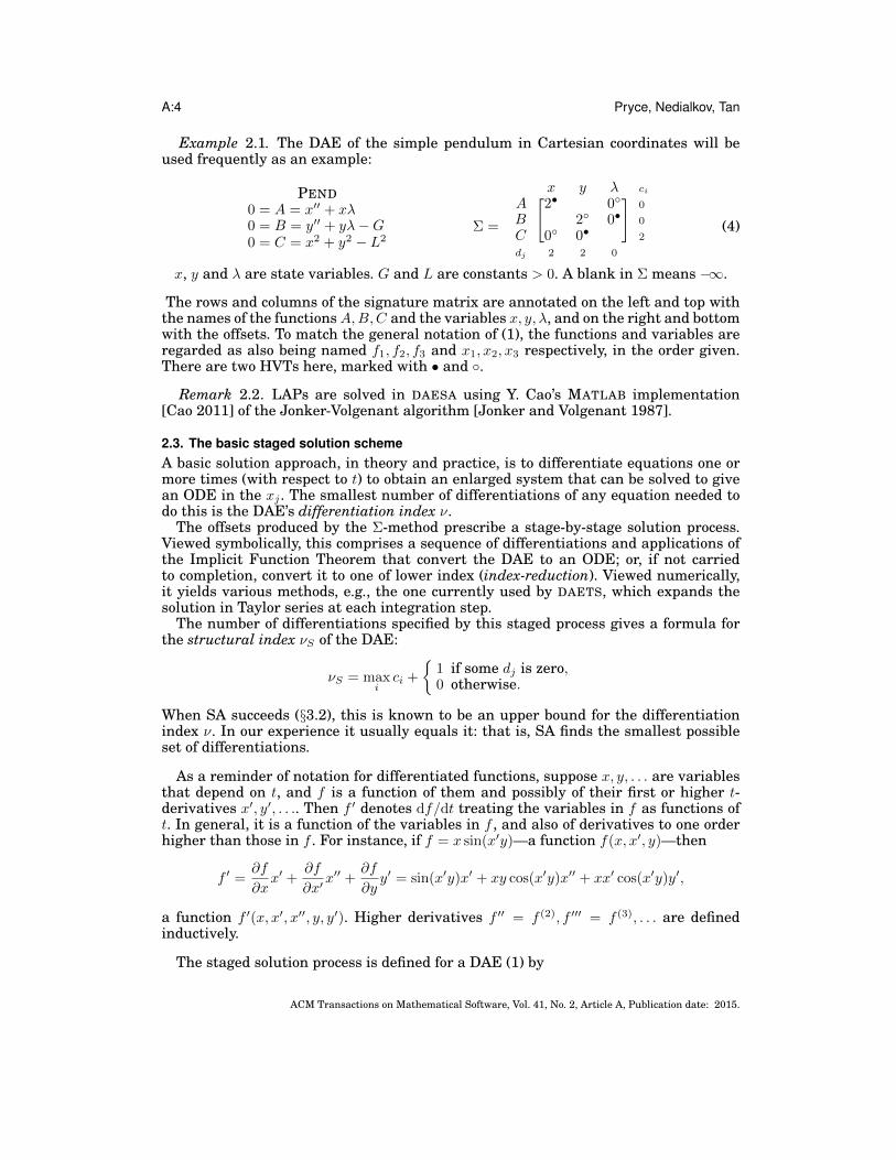
Example 2.1. The DAE of the simple pendulum in Cartesian coordinates will beused frequently as an example:
PEND0 = A = x′′ + xλ0 = B = y′′ + yλ−G0 = C = x2 + y2 − L2
Σ =
x y λ ci[ ]A 2• 0◦ 0
B 2◦ 0• 0
C 0◦ 0• 2
dj 2 2 0
(4)
x, y and λ are state variables. G and L are constants > 0. A blank in Σ means −∞.
The rows and columns of the signature matrix are annotated on the left and top withthe names of the functionsA,B,C and the variables x, y, λ, and on the right and bottomwith the offsets. To match the general notation of (1), the functions and variables areregarded as also being named f1, f2, f3 and x1, x2, x3 respectively, in the order given.There are two HVTs here, marked with • and ◦.
Remark 2.2. LAPs are solved in DAESA using Y. Cao’s MATLAB implementation[Cao 2011] of the Jonker-Volgenant algorithm [Jonker and Volgenant 1987].
2.3. The basic staged solution schemeA basic solution approach, in theory and practice, is to differentiate equations one ormore times (with respect to t) to obtain an enlarged system that can be solved to givean ODE in the xj . The smallest number of differentiations of any equation needed todo this is the DAE’s differentiation index ν.
The offsets produced by the Σ-method prescribe a stage-by-stage solution process.Viewed symbolically, this comprises a sequence of differentiations and applications ofthe Implicit Function Theorem that convert the DAE to an ODE; or, if not carriedto completion, convert it to one of lower index (index-reduction). Viewed numerically,it yields various methods, e.g., the one currently used by DAETS, which expands thesolution in Taylor series at each integration step.
The number of differentiations specified by this staged process gives a formula forthe structural index νS of the DAE:
νS = maxici +
{1 if some dj is zero,0 otherwise.
When SA succeeds (§3.2), this is known to be an upper bound for the differentiationindex ν. In our experience it usually equals it: that is, SA finds the smallest possibleset of differentiations.
As a reminder of notation for differentiated functions, suppose x, y, . . . are variablesthat depend on t, and f is a function of them and possibly of their first or higher t-derivatives x′, y′, . . .. Then f ′ denotes df/dt treating the variables in f as functions oft. In general, it is a function of the variables in f , and also of derivatives to one orderhigher than those in f . For instance, if f = x sin(x′y)—a function f(x, x′, y)—then
f ′ =∂f
∂xx′ +
∂f
∂x′x′′ +
∂f
∂yy′ = sin(x′y)x′ + xy cos(x′y)x′′ + xx′ cos(x′y)y′,
a function f ′(x, x′, x′′, y, y′). Higher derivatives f ′′ = f (2), f ′′′ = f (3), . . . are definedinductively.
The staged solution process is defined for a DAE (1) by
ACM Transactions on Mathematical Software, Vol. 41, No. 2, Article A, Publication date: 2015.
DAESA— a MATLAB Tool for Structural Analysis of DAEs A:5
Starting with k = −max dj , in order of increasing stage number k,
solve the equations f(k+ci)i = 0 for those i such that k + ci ≥ 0 (5)
for the unknowns x(k+dj)j for those j such that k + dj ≥ 0. (6)
This deceptively simple rule needs explanation. Define mk and nk to be the number ofnon-negative k + ci, and k + dj , respectively, so that (5, 6) specify mk equations in nkunknowns.
For k < kc := −maxi ci, there are no equations to solve (mk = 0), and for k < kd :=−maxj dj there are no unknowns to solve for (nk = 0). Since all finite σij are ≥ 0, itfollows from (2) that kd ≤ kc ≤ 0 (and kd < 0, except in the special case that the DAEis a purely algebraic system). Thus the solution process starts at stage k = kd.
It is immediate from their definition that the mk and nk increase with k, with mk ≤nk for all k, and mk = nk = n when k ≥ 0.
The variables and derivatives found at a given stage occur (usually) in the equa-tions at all later stages. Thus, globally over all the stages, the equations have a block-triangular structure that is solved by block forward substitution: known values fromprevious stages are substituted into the mk equations (5) of the current stage, leavingjust the nk items (6) to solve for.
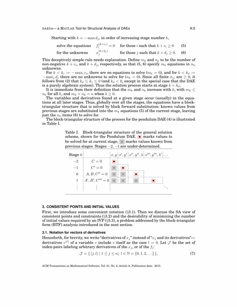
The block-triangular structure of the process for the pendulum DAE (4) is illustratedin Table I.
Table I. Block-triangular structure of the general solutionscheme, shown for the Pendulum DAE. • marks values tobe solved for at current stage; × marks values known fromprevious stages. Stages −2,−1 are under-determined.
Stage k x, y x′, y′ x′′, y′′, λ x′′′, y′′′, λ′ . . .
−2 C = 0 •−1 C ′ = 0 × •
0 A,B,C ′′ = 0 × × •1 A′, B′, C ′′′ = 0 × × × •...
.... . .
3. CONSISTENT POINTS AND INITIAL VALUESFirst, we introduce some convenient notation (§3.1). Then we discuss the SA view ofconsistent points and constraints (§3.2) and the desirability of minimizing the numberof initial values required by an IVP (§3.3), a problem addressed by the block-triangularform (BTF) analysis introduced in the next section.
3.1. Notation for vectors of derivativesHenceforth, for brevity, we write “derivatives of xj” instead of “xj and its derivatives”—derivatives v(l) of a variable v include v itself as the case l = 0. Let J be the set ofindex-pairs labeling arbitrary derivatives of the xj , or of the fi:
J = { (j, l) | 1 ≤ j ≤ n; l ∈ N = {0, 1, 2, . . .} }, (7)
ACM Transactions on Mathematical Software, Vol. 41, No. 2, Article A, Publication date: 2015.
A:6 Pryce, Nedialkov, Tan
A vector of specified derivatives of state variables of (1) can be denoted as xJ for somefinite subset J of J , meaning the vector of all derivatives x(l)j for (j, l) ∈ J ; it may benumeric, or symbolic, or a vector function xJ(t), depending on context.
For a DAE with individually named variables, such as the pendulum (4), we use anatural notation for vectors x of derivatives: for instance we may consider the vector
x = (x, x′, y, y′).
This converts to the general notation thus: since x, y are x1, x2, we have
x =(x(0)1 , x
(1)1 , x
(0)2 , x
(1)2
),
so
x = xJ , J = {(1, 0), (1, 1), (2, 0), (2, 1)} ⊂ J .
Similarly, the vector of functions
(A,B,C ′′) = (f(0)1 , f
(0)2 , f
(2)3 ) = fI , where I = {(1, 0), (2, 0), (3, 2)} ⊂ J .
3.2. The SA view of consistent pointsWe say, see [Nedialkov and Pryce 2005, §4.4], that solutions of the DAE live in xJspace, if there is at most one solution having given values of the derivatives specifiedby xJ at t = 0—or at a given t, if the DAE is non-autonomous, i.e., if t occurs explicitlyin it. We assume that the same J will do for all points along a solution path and for allsolution paths (however many DAEs have “switching” behavior that violates this). Letus call an xJ space a home, if the DAE lives in it. A home is not unique: any “larger”space (an xJ′ space with J ′ ⊃ J) has the same property.
Finding a home space amounts to finding what derivatives x(l)j must be given IVs todefine a unique solution, as argued in §3.3. So it is an important user-interface issue.
A point of a home space through which a solution of the DAE exists is called aconsistent point. The set M of all consistent points is the consistent manifold for thisspace. Equations of whichM is the zero-set are constraints of the DAE for this space.
Crucial for our solution method is the DAE’s n×n System Jacobian matrix J, where
Jij =∂fi
∂x(dj−ci)j
=
∂fi
∂x(σij)j
if dj − ci = σij , and
0 otherwise.
If there exists a consistent point at which J is nonsingular, then there is a solution ofthe DAE through it, at least locally, and we say the SA succeeds; otherwise it fails. Inour experience, SA succeeds in most practical applications, but not all.
The problem of checking for success numerically is similar to that of finding a con-sistent point to start integrating an IVP, with the difference that there are no user-specified IVs to keep “close” to: any point will do that satisfies the consistency equa-tions and has J nonsingular. Currently DAESA does not do a numerical success check.We aim to offer this in a future version.
When SA succeeds (and along the thus defined solution path), the equations (5, 6)form, for each k > 0, a square nonsingular linear system whose matrix is J, whichtherefore has a unique solution. This also holds for k = 0 in the common case that theDAE is quasilinear, that is, the x(dj)j for j = 1, . . . , n, occur linearly (or are absent) in fifor i = 1, . . . , n.
ACM Transactions on Mathematical Software, Vol. 41, No. 2, Article A, Publication date: 2015.
DAESA— a MATLAB Tool for Structural Analysis of DAEs A:7
That is, once one has solved all stages k ≤ 0 (k < 0 if quasilinear), the solution isuniquely determined. Equivalently, one does not need to look for a home space largerthan xJ≤0
, or xJ<0 if quasilinear, where the index sets
J≤0 = { (j, l) | j = 1, . . . , n; l = 0, . . . , dj } andJ<0 = { (j, l) | j = 1, . . . , n; l = 0, . . . , dj−1 } (8)
list the x(l)j solved for in stages k ≤ 0, and k < 0, respectively. Further, the constraintsthat define M are the set of equations fI≤0
= 0, when solutions live in xJ≤0space, or
fI<0 = 0, when solutions live in xJ<0 space, where
I≤0 = { (i, l) | i = 1, . . . , n; l = 0, . . . , ci } andI<0 = { (i, l) | i = 1, . . . , n; l = 0, . . . , ci−1 } (9)
list the f (l)i solved for in stages k ≤ 0, and k < 0, respectively.
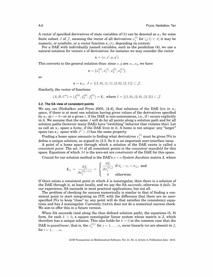
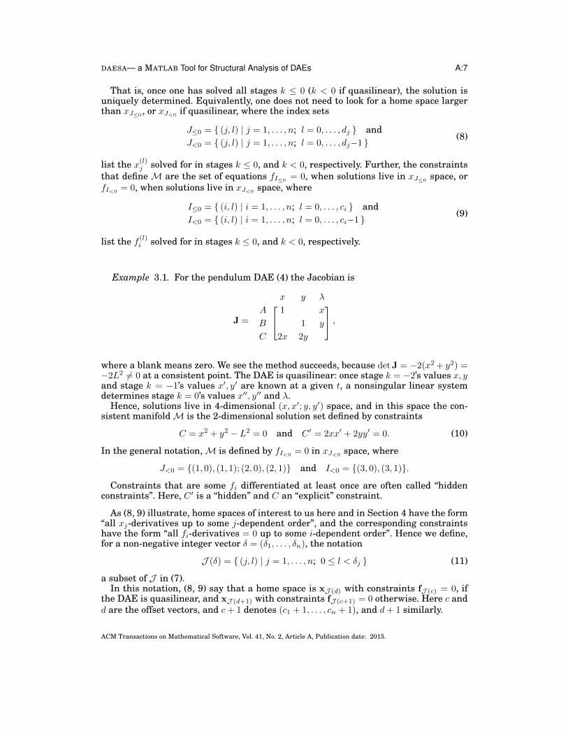
Example 3.1. For the pendulum DAE (4) the Jacobian is
J =
x y λ A 1 x
B 1 y
C 2x 2y
,
where a blank means zero. We see the method succeeds, because detJ = −2(x2 + y2) =−2L2 6= 0 at a consistent point. The DAE is quasilinear: once stage k = −2’s values x, yand stage k = −1’s values x′, y′ are known at a given t, a nonsingular linear systemdetermines stage k = 0’s values x′′, y′′ and λ.
Hence, solutions live in 4-dimensional (x, x′; y, y′) space, and in this space the con-sistent manifoldM is the 2-dimensional solution set defined by constraints
C = x2 + y2 − L2 = 0 and C ′ = 2xx′ + 2yy′ = 0. (10)
In the general notation,M is defined by fI<0= 0 in xJ<0
space, where
J<0 = {(1, 0), (1, 1); (2, 0), (2, 1)} and I<0 = {(3, 0), (3, 1)}.
Constraints that are some fi differentiated at least once are often called “hiddenconstraints”. Here, C ′ is a “hidden” and C an “explicit” constraint.
As (8, 9) illustrate, home spaces of interest to us here and in Section 4 have the form“all xj-derivatives up to some j-dependent order”, and the corresponding constraintshave the form “all fi-derivatives = 0 up to some i-dependent order”. Hence we define,for a non-negative integer vector δ = (δ1, . . . , δn), the notation
J (δ) = { (j, l) | j = 1, . . . , n; 0 ≤ l < δj } (11)
a subset of J in (7).In this notation, (8, 9) say that a home space is xJ (d) with constraints fJ (c) = 0, if
the DAE is quasilinear, and xJ (d+1) with constraints fJ (c+1) = 0 otherwise. Here c andd are the offset vectors, and c+ 1 denotes (c1 + 1, . . . , cn + 1), and d+ 1 similarly.
ACM Transactions on Mathematical Software, Vol. 41, No. 2, Article A, Publication date: 2015.
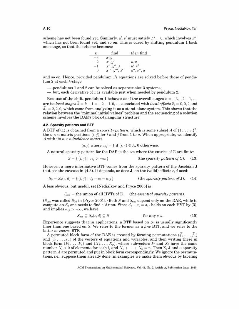
A:8 Pryce, Nedialkov, Tan
3.3. Minimizing the set of initial valuesHow should a user specify a numerical IVP? Ideally, by giving an exact consistentpoint: numerical values for some collection of derivatives, such that there is one andonly one solution taking these values at the initial t. However, it is notoriously hardto make even a good guess at consistent values, especially of derivatives, so one wouldlike an IVP code to minimize the number of IVs2: to ask the user for an x∗J where |J |,the number of elements in J , is a minimum given that solutions live in xJ space.
Typically a code then finds a nearby xJ that is consistent (within a tolerance).E.g., for the pendulum, given a numerical x∗J = (x∗, y∗, (x′)∗, (y′)∗) it might seekxJ = (x, y, x′, y′) that minimizes ‖xJ − x∗J‖ in some norm subject to the constraints(10) that defineM.
Common sense, and the stage-wise form of the solution process (5, 6), suggest theIVs should not include a derivative of some variable, if there is a lower derivative of thesame variable that is not included. E.g., for the pendulum, maybe values for x, x′′, y′, λspecify a unique solution, but these are not sensible IVs to ask of a user.
Hence, we restrict attention to IV data of the form xJ (δ) as in (11). Since |J (δ)| =∑j δj , we pose the problem thus:
Seek a home space xJ (δ) with minimum∑j δj .
As seen above, we can take δ to be d in the quasilinear case, and d+1 otherwise. How-ever, for most DAEs in applications, this is far from minimizing
∑j δj . These global off-
sets dj should be replaced by the local offsets dj derived from BTF analysis as discussedin Section 4.
Remark 3.2. Most current DAE codes do not have this ability to be selective aboutthe IVs needed for a particular problem. E.g., the code DASSL requires “flat” data com-prising all variables (x1, . . . , xn) and all first derivatives (x′1, . . . , x
′n). This corresponds
to δ = (2, 2, . . . , 2) in the J (δ) notation.
Remark 3.3. Using the equations to reduce the IVs needed. At stage k there are nkunknowns (derivatives) to find, which must satisfy mk ≤ nk equations. Often mk = 0,in which case the unknowns are genuinely arbitrary initial values, as for an ODE.However when mk > 0, there is the possibility of specifying nk − mk values—and/orconstraints of another kind—sufficient to determine all nk unknowns uniquely. E.g.,suppose the pendulum DAE has L = 10. At stage −2 with m−2 = 1 equation x2 + y2 −102 = 0 to solve for n−2 = 2 unknowns x, y, one could specify that x = 6 is fixed, plusthe constraint y < 0. This suffices to fix y = −8 uniquely. One can do similarly at stage−1. In general, nk−mk is “the number of DOF introduced at stage k”, and its sum overk < 0 is the total DOF of the system.
If done for all stages < 0 and based on BTF analysis, this approach has the meritof requiring exactly as many IVs as there are DOF, but software must take care toavoid problems of conditioning (in the above example, y is ill-determined when x isjust under 10), existence (there is no y when x > 10) and uniqueness (one must knowwhat constraints like “y < 0” to impose). Therefore we regard this idea as an issue ofuser interface, not of the theory presented here, and do not pursue it further.
4. BLOCK-TRIANGULAR FORM WITHIN THE DAEWe illustrate how “superfluous” IVs are suggested by the original Σ-method (§4.1),and show how block-triangular form (BTF), based on various sparsity patterns derived
2IV means both known initial values and also trial values, guesses at the solution of an equation system.
ACM Transactions on Mathematical Software, Vol. 41, No. 2, Article A, Publication date: 2015.
DAESA— a MATLAB Tool for Structural Analysis of DAEs A:9
from the DAE, can reduce the number of IVs (§4.2, §4.3). We discuss irreducible BTFbased on the Jacobian sparsity and the associated local offsets (§4.4, §4.5). Its synergywith quasilinearity analysis often reduces the number of IVs still further (§4.6).
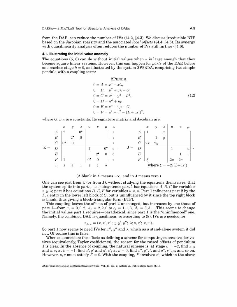
4.1. Illustrating the initial value anomalyThe equations (5, 6) can do without initial values when k is large enough that theybecome square linear systems. However, this can happen for parts of the DAE beforeone reaches stage k = 0, as illustrated by the system 2PENDA, comprising two simplependula with a coupling term:
2PENDA0 = A = x′′ + xλ,
0 = B = y′′ + yλ−G,0 = C = x2 + y2 − L2,
0 = D = u′′ + uµ,
0 = E = v′′ + vµ−G,0 = F = u2 + v2 − (L+ cx′)2,
(12)
where G,L, c are constants. Its signature matrix and Jacobian are
Σ =
x y λ u v µ ci
A 2 0• 1
B 2• 0 1
C 0• 0 3
D 2 0• 0
E 2• 0 0
F 1 0• 0 2
dj 3 3 1 2 2 0
, J =
x y λ u v µ
A 1 x
B 1 y
C 2x 2y
D 1 u
E 1 v
F ξ 2u 2v
where ξ = −2c(L+cx′)
.
(A blank in Σ means −∞, and in J means zero.)
One can see just from Σ (or from J), without studying the equations themselves, thatthe system splits into parts, i.e., subsystems: part 1 has equations A,B,C for variablesx, y, λ; part 2 has equations D,E, F for variables u, v, µ. Part 1 influences part 2 by theF, x entry in the lower left block of Σ, but is uninfluenced by it since the top right blockis blank, thus giving a block-triangular form (BTF).
This coupling leaves the offsets of part 2 unchanged, but increases by one those ofpart 1—from ci = 0, 0, 2, dj = 2, 2, 0 to ci = 1, 1, 3, dj = 3, 3, 1. This seems to changethe initial values part 1 requires—paradoxical, since part 1 is the “uninfluenced” one.Namely, the combined DAE is quasilinear, so according to (8), IVs are needed for
xJ<0= (x, x′, x′′; y, y′, y′′; λ;u, u′; v, v′).
So part 1 now seems to need IVs for x′′, y′′ and λ, which as a stand-alone system it didnot. Of course this is false.
When one considers the offsets as defining a scheme for computing successive deriva-tives (equivalently, Taylor coefficients), the reason for the raised offsets of pendulum1 is clear. In the absence of coupling, the natural scheme is: at stage k = −2, find x, yand u, v; at k = −1, find x′, y′ and u′, v′; at k = 0, find x′′, y′′, λ and u′′, v′′, µ; and so on.However, u, v must satisfy F = 0. With the coupling, F involves x′, which in the above
ACM Transactions on Mathematical Software, Vol. 41, No. 2, Article A, Publication date: 2015.
A:10 Pryce, Nedialkov, Tan
scheme has not been found yet. Similarly, u′, v′ must satisfy F ′ = 0, which involves x′′,which has not been found yet, and so on. This is cured by shifting pendulum 1 backone stage, so that the scheme becomes:
k find then find−3 x, y−2 x′, y′ u, v−1 x′′, y′′, λ u′, v′
0 x′′′, y′′′, λ′ u′′, v′′, µ
and so on. Hence, provided pendulum 1’s equations are solved before those of pendu-lum 2 at each k-stage,
— pendulums 1 and 2 can be solved as separate size 3 systems;— but, each derivative of x is available just when needed by pendulum 2.
Because of the shift, pendulum 1 behaves as if the overall stages k = −3,−2,−1, . . .
are its local stages k = k + 1 = −2,−1, 0, . . . associated with local offsets ci = 0, 0, 2 anddj = 2, 2, 0, which come from analyzing it as a stand-alone system. This shows that therelation between the “minimal initial values” problem and the sequencing of a solutionscheme involves the DAE’s block-triangular structure.
4.2. Sparsity patterns and BTFA BTF of (1) is obtained from a sparsity pattern, which is some subset A of {1, . . . , n}2,the n × n matrix positions (i, j) for i and j from 1 to n. When appropriate, we identifyA with its n× n incidence matrix
(aij) where aij = 1 if (i, j) ∈ A, 0 otherwise.
A natural sparsity pattern for the DAE is the set where the entries of Σ are finite:
S = { (i, j) | σij > −∞} (the sparsity pattern of Σ). (13)
However, a more informative BTF comes from the sparsity pattern of the Jacobian J(but see the caveats in §4.3). It depends, as does J, on the (valid) offsets c, d used:
S0 = S0(c, d) = { (i, j) | dj − ci = σij } (the sparsity pattern of J). (14)
A less obvious, but useful, set [Nedialkov and Pryce 2005] is
Sess = the union of all HVTs of Σ. (the essential sparsity pattern).
(Sess was called S00 in [Pryce 2001].) Both S and Sess depend only on the DAE, while tocompute an S0 one needs to find c, d first. Since dj − ci = σij holds on each HVT by (3),and implies σij > −∞, we have
Sess ⊆ S0(c, d) ⊆ S for any c, d. (15)
Experience suggests that in applications, a BTF based on S0 is usually significantlyfiner than one based on S. We refer to the former as a fine BTF, and we refer to thelatter as coarse BTF.
A permuted block form of the DAE is created by forming permutations (f1, . . . , fn)and (x1, . . . , xn) of the vectors of equations and variables, and then writing these inblock form (F1, . . . , Fp) and (X1, . . . , Xp), where subvectors Fl and Xl have the samenumber Nl > 0 of elements for each l, and N1 + · · ·+Np = n. Then Σ, J and a sparsitypattern A are permuted and put in block form correspondingly. We ignore the permuta-tions, i.e., suppose them already done (in examples we make them obvious by labeling
ACM Transactions on Mathematical Software, Vol. 41, No. 2, Article A, Publication date: 2015.
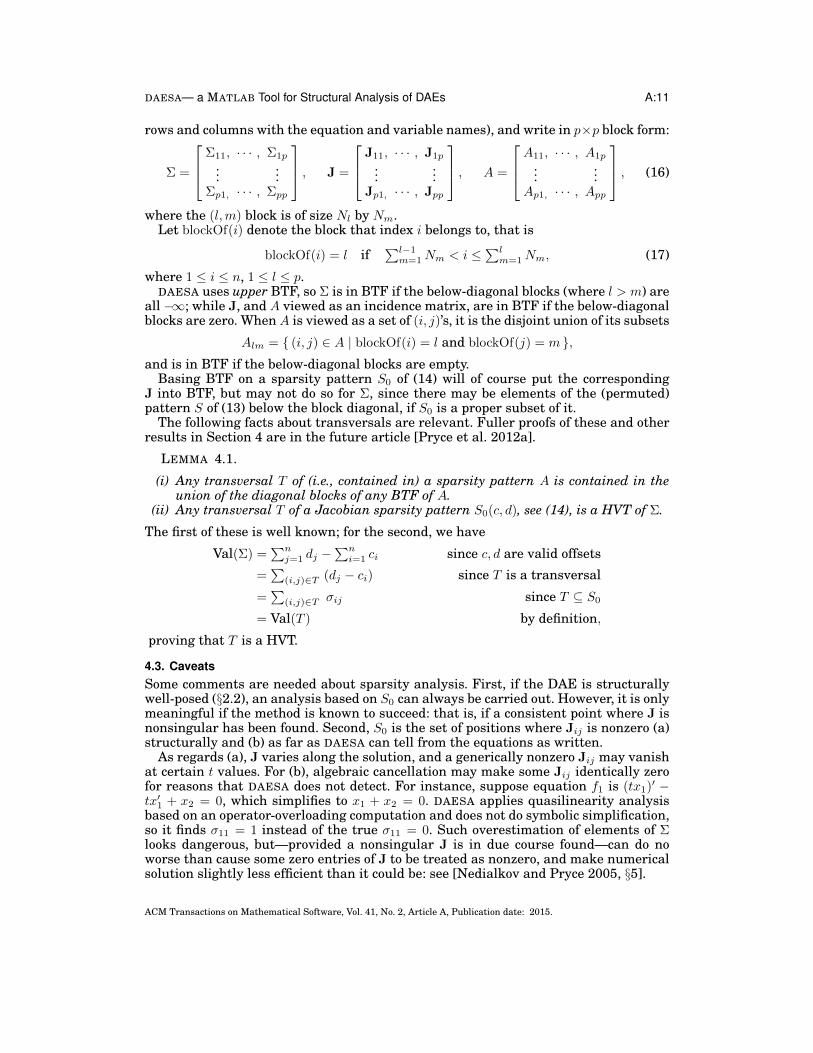
DAESA— a MATLAB Tool for Structural Analysis of DAEs A:11
rows and columns with the equation and variable names), and write in p×p block form:
Σ =
Σ11, · · · , Σ1p
......
Σp1, · · · , Σpp
, J =
J11, · · · , J1p
......
Jp1, · · · , Jpp
, A =
A11, · · · , A1p
......
Ap1, · · · , App
, (16)
where the (l,m) block is of size Nl by Nm.Let blockOf(i) denote the block that index i belongs to, that is
blockOf(i) = l if∑l−1m=1Nm < i ≤
∑lm=1Nm, (17)
where 1 ≤ i ≤ n, 1 ≤ l ≤ p.DAESA uses upper BTF, so Σ is in BTF if the below-diagonal blocks (where l > m) are
all −∞; while J, and A viewed as an incidence matrix, are in BTF if the below-diagonalblocks are zero. When A is viewed as a set of (i, j)’s, it is the disjoint union of its subsets
Alm = { (i, j) ∈ A | blockOf(i) = l and blockOf(j) = m },and is in BTF if the below-diagonal blocks are empty.
Basing BTF on a sparsity pattern S0 of (14) will of course put the correspondingJ into BTF, but may not do so for Σ, since there may be elements of the (permuted)pattern S of (13) below the block diagonal, if S0 is a proper subset of it.
The following facts about transversals are relevant. Fuller proofs of these and otherresults in Section 4 are in the future article [Pryce et al. 2012a].
LEMMA 4.1.
(i) Any transversal T of (i.e., contained in) a sparsity pattern A is contained in theunion of the diagonal blocks of any BTF of A.
(ii) Any transversal T of a Jacobian sparsity pattern S0(c, d), see (14), is a HVT of Σ.
The first of these is well known; for the second, we have
Val(Σ) =∑nj=1 dj −
∑ni=1 ci since c, d are valid offsets
=∑
(i,j)∈T (dj − ci) since T is a transversal
=∑
(i,j)∈T σij since T ⊆ S0
= Val(T ) by definition,
proving that T is a HVT.
4.3. CaveatsSome comments are needed about sparsity analysis. First, if the DAE is structurallywell-posed (§2.2), an analysis based on S0 can always be carried out. However, it is onlymeaningful if the method is known to succeed: that is, if a consistent point where J isnonsingular has been found. Second, S0 is the set of positions where Jij is nonzero (a)structurally and (b) as far as DAESA can tell from the equations as written.
As regards (a), J varies along the solution, and a generically nonzero Jij may vanishat certain t values. For (b), algebraic cancellation may make some Jij identically zerofor reasons that DAESA does not detect. For instance, suppose equation f1 is (tx1)′ −tx′1 + x2 = 0, which simplifies to x1 + x2 = 0. DAESA applies quasilinearity analysisbased on an operator-overloading computation and does not do symbolic simplification,so it finds σ11 = 1 instead of the true σ11 = 0. Such overestimation of elements of Σlooks dangerous, but—provided a nonsingular J is in due course found—can do noworse than cause some zero entries of J to be treated as nonzero, and make numericalsolution slightly less efficient than it could be: see [Nedialkov and Pryce 2005, §5].
ACM Transactions on Mathematical Software, Vol. 41, No. 2, Article A, Publication date: 2015.
A:12 Pryce, Nedialkov, Tan
4.4. IrreducibilityAn n × n sparsity pattern A (or matrix) is irreducible, if it cannot be permuted to anon-trivial BTF (one with p > 1); otherwise it is reducible.
Classic results of graph theory, see e.g. [Pothen and Fan 1990; Coleman et al. 1986],are the following. The bipartite graph of A is the undirected graph whose 2n verticesare the n rows and n columns, and which has an edge between row i and column jwhenever (i, j) ∈ A.
THEOREM 4.2.
(a) The following are equivalent:(i) A is structurally nonsingular (contains at least one transversal).
(ii) A has the Hall Property: for r = 1, . . . , n, any set of r columns of A containselements of at least r rows.
(b) The following are equivalent:(i) A is irreducible.
(ii) A has the Strong Hall Property: for r = 1, . . . , n − 1, any set of r columns of Acontains elements of at least r + 1 rows.
(iii) Every element of A is on a transversal, and the bipartite graph of A is con-nected.
Clearly, if any diagonal block All of a BTF of A is reducible (as a sparsity patternin its own right), this lets one refine the whole BTF of A, splitting the lth block intotwo or more smaller blocks. Repeating this as needed, A has a BTF for which eachdiagonal block is irreducible, which we call an irreducible BTF of A. This is unique upto possible reordering of the blocks, [Duff et al. 1986].
The ⊆ part of the following result comes from Lemma 4.1(i,ii) and the definition ofSess. The ⊇ part comes from the fact, which uses Theorem 4.2 (b)(iii), that each elementof each diagonal block (Sll) is on a transversal.
THEOREM 4.3. For a given signature matrix Σ, let (Slm) be an irreducible BTF of aJacobian sparsity pattern S0 = S0(c, d); that is,
Slm = { (i, j) ∈ S0 | blockOf(i) = l and blockOf(j) = m }.
Then the essential sparsity pattern Sess is exactly the union of the diagonal blocks,
Sess = S11 ∪ . . . ∪ Spp.
It follows that, up to possible reordering, all Jacobian sparsity patterns S0(c, d) of Σhave the same block sizes N1, . . . , Np, and indeed identical diagonal blocks, in theirirreducible BTFs. Depending on the DAE, some ordering of blocks may be arbitrary;some may be dictated by a specific choice of offsets c and d; some may be inherent inthe DAE. This is studied in [Pryce et al. 2012a].
4.5. BTF, local offsets, and solution schemeFor any BTF (16) of a DAE, local offsets of part l (l = 1, . . . , p) are offsets obtained bystructural analysis of Σll, i.e., by treating part l as a free-standing DAE, with knowndriving terms coming from any coupling to parts l+1, . . . , p. Since we are ignoringthe permutations, we write a set of global offsets—arbitrary valid offsets of Σ as awhole—as c1, . . . , cn and d1, . . . , dn in the order of the permuted matrices in (16); andthe canonical local offsets as c1, . . . , cn and d1, . . . , dn in the same way. (E.g., d1, . . . , dN1
and d1, . . . , dN1are the global and local offsets of the variables of part 1 of the DAE,
and so on.)
ACM Transactions on Mathematical Software, Vol. 41, No. 2, Article A, Publication date: 2015.
DAESA— a MATLAB Tool for Structural Analysis of DAEs A:13
From [Pryce et al. 2012a] we have the following, whose proof relies on Theorem 4.2(b)(iii): an irreducible pattern has a connected bipartite graph.
THEOREM 4.4. Consider the irreducible BTF in of the Jacobian sparsity patternS0(c, d) for any valid (global) offsets c, d. Then the difference between global and localoffsets is constant on each block. That is, there are non-negative integersK1, . . . ,Kp suchthat
cj − cj = dj − dj = Kl where l = blockOf(j), see (17).
Consider (5, 6) as a Taylor series generation scheme. Using the fine BTF, one canregard part l for l = 1, . . . , p as a separate DAE, possibly receiving driving terms fromparts l + 1, . . . , p, the process being interleaved so that at each k-stage, needed Taylorcoefficients are available for substitution into the equations just when they are needed.
Theorem 4.4 shows that this works, because each part behaves as if its private solu-tion scheme, including the negative stages, is the same as if it were free-standing usingits local offsets, but shifted Kl stages earlier. In particular, each part only requires theIVs that are specified by its local offsets. In future article [Nedialkov et al. 2014] weprove, with the notation and assumptions of §3.3:
THEOREM 4.5. The minimal vector xJ (δ) of initial values of the DAE is based onthe canonical local offsets, namely the vector δ is given by
δj =
{dj if part blockOf(j) of the DAE is quasilinear,
dj + 1 otherwise.(18)
The number Kl can be viewed as a “lead time” given to each k-stage of part l of theDAE to ensure successful interleaving.
A detailed solution scheme, which is the refinement of (5, 6) based on the irre-ducible blocks of S0 together with quasilinearity analysis, is displayed by DAESA’sprintSolScheme function. It gives valuable insight into the DAE and suggests waysto improve computational efficiency.
4.6. Quasilinearity and local quasilinearityThe quasilinearity referred to in (18) is of course local, meaning that part l is quasi-linear regarded as a free-standing DAE—that is, the djth derivative of xj , for all jbelonging to block l, occurs linearly (or is absent) in fi for all i belonging to block l.
Local quasilinearity occurs frequently, which is one reason why linearity analysisand BTF analysis together are more effective than either separately at reducing thenumber of IVs required. We call the DAE as a whole locally quasilinear, if each blockin the irreducible BTF based on S0 is locally quasilinear. Since these blocks are thesame as those of Sess by Theorem 4.3, this is a well-defined property independent ofthe (global) offsets c, d used to define S0.
[Nedialkov et al. 2014] describes the algorithms used in DAETS and DAESA to deter-mine quasilinearity.
5. SOME EXAMPLESWe give some examples to illustrate these ideas. The facts reported were confirmedusing DAESA.
For a notation independent of permutations, matrix entries and offsets in theseexamples are labeled by their equation and/or variable instead of numerically, e.g.,cA, cB , . . ., dx, dy, . . ., σA,x , . . . instead of c1, c2, . . ., d1, d2, . . ., σ11, . . ..
ACM Transactions on Mathematical Software, Vol. 41, No. 2, Article A, Publication date: 2015.
A:14 Pryce, Nedialkov, Tan
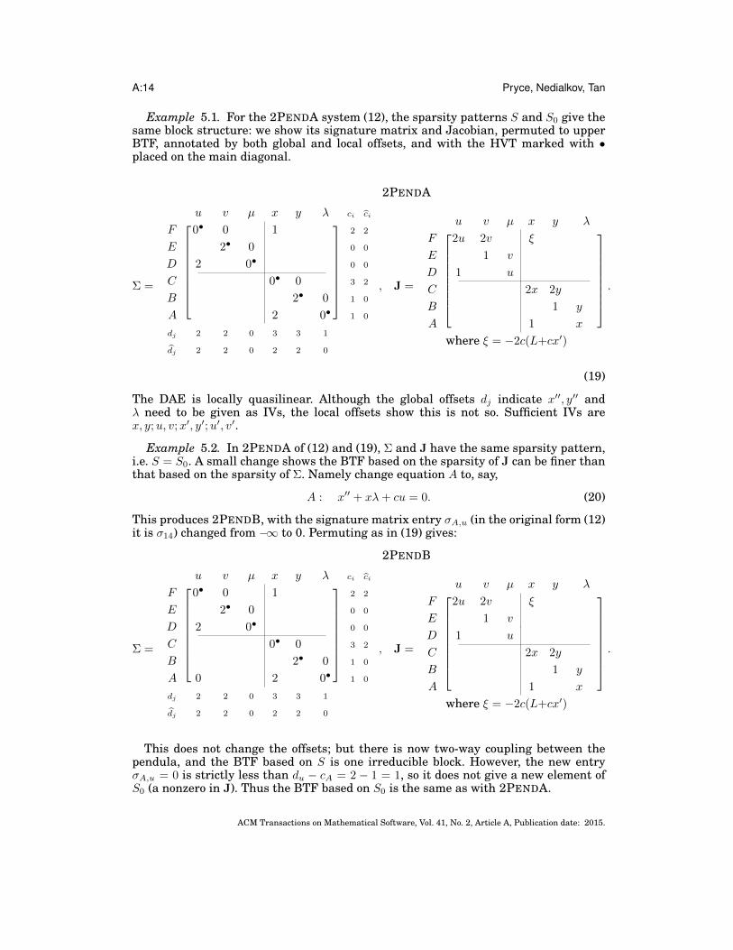
Example 5.1. For the 2PENDA system (12), the sparsity patterns S and S0 give thesame block structure: we show its signature matrix and Jacobian, permuted to upperBTF, annotated by both global and local offsets, and with the HVT marked with •placed on the main diagonal.
2PENDA
Σ =
u v µ x y λ ci ci
F 0• 0 1 2 2
E 2• 0 0 0
D 2 0• 0 0
C 0• 0 3 2
B 2• 0 1 0
A 2 0• 1 0
dj 2 2 0 3 3 1
dj 2 2 0 2 2 0
, J =
u v µ x y λ
F 2u 2v ξ
E 1 v
D 1 u
C 2x 2y
B 1 y
A 1 x
where ξ = −2c(L+cx′)
.
(19)
The DAE is locally quasilinear. Although the global offsets dj indicate x′′, y′′ andλ need to be given as IVs, the local offsets show this is not so. Sufficient IVs arex, y;u, v;x′, y′;u′, v′.
Example 5.2. In 2PENDA of (12) and (19), Σ and J have the same sparsity pattern,i.e. S = S0. A small change shows the BTF based on the sparsity of J can be finer thanthat based on the sparsity of Σ. Namely change equation A to, say,
A : x′′ + xλ+ cu = 0. (20)
This produces 2PENDB, with the signature matrix entry σA,u (in the original form (12)it is σ14) changed from −∞ to 0. Permuting as in (19) gives:
2PENDB
Σ =
u v µ x y λ ci ci
F 0• 0 1 2 2
E 2• 0 0 0
D 2 0• 0 0
C 0• 0 3 2
B 2• 0 1 0
A 0 2 0• 1 0
dj 2 2 0 3 3 1
dj 2 2 0 2 2 0
, J =
u v µ x y λ
F 2u 2v ξ
E 1 v
D 1 u
C 2x 2y
B 1 y
A 1 x
where ξ = −2c(L+cx′)
.
This does not change the offsets; but there is now two-way coupling between thependula, and the BTF based on S is one irreducible block. However, the new entryσA,u = 0 is strictly less than du − cA = 2 − 1 = 1, so it does not give a new element ofS0 (a nonzero in J). Thus the BTF based on S0 is the same as with 2PENDA.
ACM Transactions on Mathematical Software, Vol. 41, No. 2, Article A, Publication date: 2015.
DAESA— a MATLAB Tool for Structural Analysis of DAEs A:15
As a DAE, pendulum 1 still drives pendulum 2—the reverse effect is too weak tochange the solution scheme’s block structure. Therefore the local offsets are also un-changed, and x, y;u, v;x′, y′;u′, v′ still suffice as IVs.
Example 5.3. Now consider 2PENDC, in which the cu term in (20) is changed to cu′.This still does not change the global offsets; but now σA,u = 1 = du − cA, so J has a(structural) nonzero here, namely JA,u = c, and the two-way coupling is stronger. NowS0 = S, and the BTF based on S0 is one irreducible block.
Thus the local offsets are now the same as the global ones; each solution stage(for k ≥ 0) entails solving a 6 × 6 linear system instead of two 3 × 3 ones; andx, y;u, v;x′, y′;u′, v′ no longer suffice as IVs—one must provide x′′, y′′ and λ also.
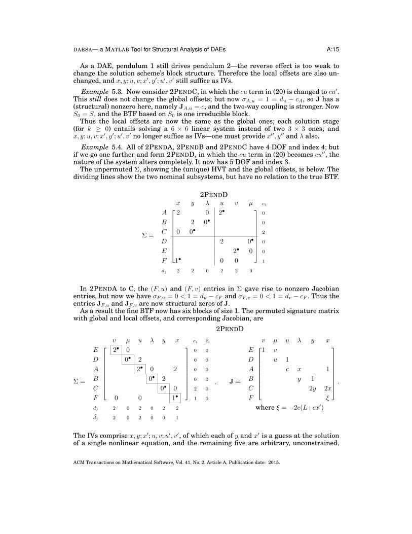
Example 5.4. All of 2PENDA, 2PENDB and 2PENDC have 4 DOF and index 4; butif we go one further and form 2PENDD, in which the cu term in (20) becomes cu′′, thenature of the system alters completely. It now has 5 DOF and index 3.
The unpermuted Σ, showing the (unique) HVT and the global offsets, is below. Thedividing lines show the two nominal subsystems, but have no relation to the true BTF.
Σ =
2PENDDx y λ u v µ ci
A 2 0 2• 0
B 2 0• 0
C 0 0• 2
D 2 0• 0
E 2• 0 0
F 1• 0 0 1
dj 2 2 0 2 2 0
In 2PENDA to C, the (F, u) and (F, v) entries in Σ gave rise to nonzero Jacobianentries, but now we have σF,u = 0 < 1 = du − cF and σF,v = 0 < 1 = dv − cF . Thus theentries JF,u and JF,v are now structural zeros of J.
As a result the fine BTF now has six blocks of size 1. The permuted signature matrixwith global and local offsets, and corresponding Jacobian, are
2PENDD
Σ =
v µ u λ y x ci ci
E 2• 0 0 0
D 0• 2 0 0
A 2• 0 2 0 0
B 0• 2 0 0
C 0• 0 2 0
F 0 0 1• 1 0
dj 2 0 2 0 2 2
dj 2 0 2 0 0 1
, J =
v µ u λ y x
E 1 v
D u 1
A c x 1
B y 1
C 2y 2x
F ξ
where ξ = −2c(L+cx′)
.
The IVs comprise x, y;x′;u, v;u′, v′, of which each of y and x′ is a guess at the solutionof a single nonlinear equation, and the remaining five are arbitrary, unconstrained,
ACM Transactions on Mathematical Software, Vol. 41, No. 2, Article A, Publication date: 2015.
A:16 Pryce, Nedialkov, Tan
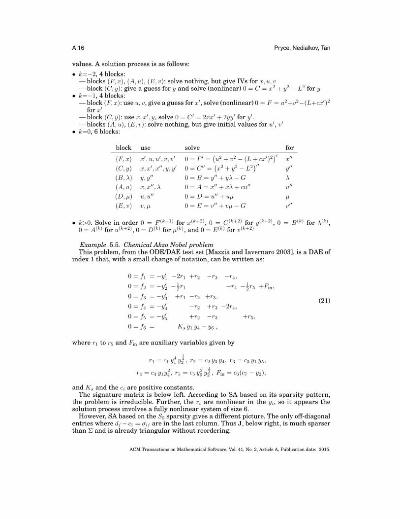
values. A solution process is as follows:• k=−2, 4 blocks:
— blocks (F, x), (A, u), (E, v): solve nothing, but give IVs for x, u, v— block (C, y): give a guess for y and solve (nonlinear) 0 = C = x2 + y2 − L2 for y
• k=−1, 4 blocks:— block (F, x): use u, v, give a guess for x′, solve (nonlinear) 0 = F = u2+v2−(L+cx′)2
for x′— block (C, y): use x, x′, y, solve 0 = C ′ = 2xx′ + 2yy′ for y′.— blocks (A, u), (E, v): solve nothing, but give initial values for u′, v′
• k=0, 6 blocks:
block use solve for
(F, x) x′, u, u′, v, v′ 0 = F ′ =(u2 + v2 − (L+ cx′)2
)′x′′
(C, y) x, x′, x′′, y, y′ 0 = C ′′ =(x2 + y2 − L2
)′′y′′
(B, λ) y, y′′ 0 = B = y′′ + yλ−G λ
(A, u) x, x′′, λ 0 = A = x′′ + xλ+ cu′′ u′′
(D,µ) u, u′′ 0 = D = u′′ + uµ µ
(E, v) v, µ 0 = E = v′′ + vµ−G v′′
• k>0. Solve in order 0 = F (k+1) for x(k+2), 0 = C(k+2) for y(k+2), 0 = B(k) for λ(k),0 = A(k) for u(k+2), 0 = D(k) for µ(k), and 0 = E(k) for v(k+2)
Example 5.5. Chemical Akzo Nobel problemThis problem, from the ODE/DAE test set [Mazzia and Iavernaro 2003], is a DAE of
index 1 that, with a small change of notation, can be written as:
0 = f1 = −y′1 −2r1 +r2 −r3 −r4,0 = f2 = −y′2 − 1
2r1 −r4 − 12r5 +Fin,
0 = f3 = −y′3 +r1 −r2 +r3,
0 = f4 = −y′4 −r2 +r3 −2r4,
0 = f5 = −y′5 +r2 −r3 +r5,
0 = f6 = Ks y1 y4 − y6 ,
(21)
where r1 to r5 and Fin are auxiliary variables given by
r1 = c1 y41 y
122 , r2 = c2 y3 y4, r3 = c3 y1 y5,
r4 = c4 y1y24 , r5 = c5 y
26 y
122 , Fin = c6(c7 − y2),
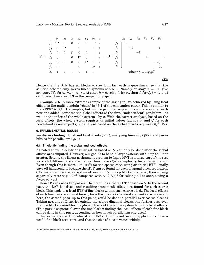
and Ks and the ci are positive constants.The signature matrix is below left. According to SA based on its sparsity pattern,
the problem is irreducible. Further, the ri are nonlinear in the yi, so it appears thesolution process involves a fully nonlinear system of size 6.
However, SA based on the S0 sparsity gives a different picture. The only off-diagonalentries where dj − ci = σij are in the last column. Thus J, below right, is much sparserthan Σ and is already triangular without reordering.
ACM Transactions on Mathematical Software, Vol. 41, No. 2, Article A, Publication date: 2015.
DAESA— a MATLAB Tool for Structural Analysis of DAEs A:17
Σ =
y1 y2 y3 y4 y5 y6 ci
f1 1• 0 0 0 0 0
f2 0 1• 0 0 0
f3 0 0 1• 0 0 0
f4 0 0 1• 0 0
f5 0 0 0 0 1• 0 0
f6 0 0 0• 0
dj 1 1 1 1 1 0
, J =
y1 y2 y3 y4 y5 y6
f1 −1
f2 −1 −ξf3 −1
f4 −1
f5 −1 2ξ
f6 −1
where ξ = c5y6y122
.
(22)
Hence the fine BTF has six blocks of size 1. In fact each is quasilinear, so that thesolution scheme only solves linear systems of size 1. Namely at stage k = −1, givearbitrary IVs for y1, y2, y3, y4, y5. At stage k = 0, solve f6 for y6, then fi for y′i, i = 1, . . . , 5(all linear). See also §5.3 in the companion paper.
Example 5.6. A more extreme example of the saving in IVs achieved by using localoffsets is the multi-pendula “chain” in §6.1 of the companion paper. This is similar tothe 2PENDA,B,C,D examples, but with p pendula coupled in such a way that eachnew one added increases the global offsets of the first, “independent” pendulum—aswell as the index of the whole system—by 2. With the correct analysis, based on thelocal offsets, the whole system requires 4p initial values (an x, y, x′ and y′ for eachpendulum) as one expects; but analysis based on the global offsets requires O(p2) IVs.
6. IMPLEMENTATION ISSUESWe discuss finding global and local offsets (§6.1), analyzing linearity (§6.2), and possi-bilities for parallelism (§6.3).
6.1. Efficiently finding the global and local offsetsAs noted above, block-triangularization based on S0 can only be done after the globaloffsets are computed. However, our goal is to handle large systems with n up to 105 orgreater. Solving the linear assignment problem to find a HVT is a large part of the costfor such DAEs—the standard algorithms have O(n3) complexity for a dense matrix.Even though this is more like O(n2) for the sparse case, using an initial BTF usuallypays off handsomely, because the HVT can be found for each diagonal block separately.(For instance, if a sparse system of size n = Np has p blocks of size N , then solvingseparately costs ≈ p · CN2 compared with ≈ C(Np)2 for solving all at once, saving afactor of ≈ p.)
Hence DAESA uses two passes. The first finds a coarse BTF based on S. In the secondpass, the LAP is solved, and resulting (canonical) offsets are found for each coarseblock. This leads to a local BTF of fine blocks within each coarse block. The local offsetsof each fine block are found here. (Since the off-block-diagonal elements are irrelevanthere, the second pass, up to this point, could be done in parallel over coarse blocks.)Taking account of Σ entries outside the coarse diagonal blocks, one further pass overthe fine blocks assembles the global offsets of the whole system from the local offsets.(This part is sequential over the fine blocks; finding the local offsets of each fine blockcan be done in this pass, depending on how much parallelism one uses.)
Our experience is that almost all DAEs of nontrivial size in applications have auseful fine block structure, and that the size of blocks varies widely.
ACM Transactions on Mathematical Software, Vol. 41, No. 2, Article A, Publication date: 2015.
A:18 Pryce, Nedialkov, Tan
For a large example, we constructed a DAE whose Σ has the sparsity pattern ofthe LHR71 matrix from the Florida collection [Davis and Hu 2011], with the finite σijbeing 0, 1 or 2 at random. The system is of size n = 70304; its block structure comprises15774 blocks of size 1, four of size 8, 154 of size in the tens, 24 of size in the hundreds,and 14 of size in the thousands, the largest being two of size 4586.
6.2. Analyzing linearityDAESA verifies whether any block of equations and variables is linear in the variablesto be solved for, using operator overloading and a variant of the automatic differentia-tion method by which the signature matrix is computed.
The analysis is made easier by some simple facts. The first, which follows from (2,5, 6), is that in any single, undifferentiated equation fi, the unknowns to be solvedfor—however the system may have been decomposed into triangular form—are alwaysa subset of the highest-order derivatives, that is of the x(σij)
j , j = 1, . . . , n. For instanceif fi involves x′2, x4 and x′′4 then x′2 and x′′4 may be among the unknowns to be solvedfor, but x4 cannot be.
The second fact is that in any function differentiated (w.r.t. t) one or more times, allthe highest derivatives occur linearly. For instance if fi is a function only of (x′2, x4, x
′′4)
then f ′i is a function only of (x′2, x′′2 , x4, x
′4, x′′4 , x′′′4 ), namely
f ′i =∂fi∂x′2
(x′2, x4, x′′4)x′′2 +
∂fi∂x4
(x′2, x4, x′′4)x′4 +
∂fi∂x′′4
(x′2, x4, x′′4)x′′′4 ,
which is linear in its highest derivatives x′′2 and x′′′4 .Hence each fi needs exactly one linearity check, at the unique stage in the sequence
(5, 6) where it occurs undifferentiated: namely for k = −ci. It is checked against the setof unknowns in its equation-block, which depends on the chosen BTF. At earlier stagesthe equation does not appear; at later ones, it appears differentiated, so is necessarilylinear.
6.3. Parallelizing the solution of IVPsFor large systems, parallel computation may be useful during the process of finding ablock-triangular form, as noted above. It also seems a promising approach for numeri-cal integration of IVPs, exploiting BTF.
One way is as follows. Some coarse BTF, based on S, is used to handle blocks ofequations by separate threads on the machine, possibly on separate processors. Letthe lth block of equations be F (l) = 0, to solve for variables X(l), l = 1, . . . , q. The off-diagonal block structure defines a directed acyclic graph: its vertices are the threads,and an edge to l from l′ > l means l uses l′, i.e., F (l) contains variables from X(l′).Each thread l is responsible for generating a sufficiently smooth piecewise polynomialrepresentation P (l)(t) of its solution function X(l)(t), and as many derivatives as maybe needed by other threads.
The threads have their own independent step size control, so that at any momentthey have in general integrated up to different points t = τ (l). Integration is advancedon demand. The process is kicked off by telling each output thread l (one which noother threads use) to integrate from t = 0 to some t = T . Each of these chooses a trialstep, say to t = h(l). This generates a demand that all blocks, which this block uses,integrate at least as far over [0, h(l)] to provide their needed polynomial approximantson this interval. These demands cascade back so that each thread, independently, ismade to integrate at least as far as the smallest of the h(l)’s over all output threads.
Once each output thread l has achieved a successful step it repeats the process untilit reaches t = T , thus forcing all other threads to integrate up to T . Such a scheme
ACM Transactions on Mathematical Software, Vol. 41, No. 2, Article A, Publication date: 2015.
DAESA— a MATLAB Tool for Structural Analysis of DAEs A:19
allows the integrators of different blocks considerable freedom. For instance one blockmight be “difficult” requiring small steps, which would not need to impact on otherblocks that might be able to take larger steps.
Such a scheme is generally not possible using a fine BTF based on S0, because l′ > lmay not imply block l′ is completely independent of block l. Thus one cannot do severalintegration steps (or even one) of l′ independently of l, by contrast with the coarse BTFcase.
7. SUMMARY OF DAESA FEATURES, AND FUTURE WORKDAESA’s facilities, given in detail in [Nedialkov et al. 2013], are outlined here. Theanalysis is begun by passing MATLAB code of the DAE to the daeSA function, whichreturns the results of its analysis in a MATLAB structure. Other functions can thenextract the information for further use in a program and/or display it, for example:
— Produce a graphical display of the signature matrix with global, and local if ap-propriate, offsets; either in its original form or permuted into the coarse BTF based onS, or the fine BTF based on S0.
— Display the refined solution scheme based on the fine BTF, indicating which setsof equations are underdetermined, which are quasilinear, etc.
— List a minimal set of derivatives required as IVs, obtained from the solutionscheme.
Taken together, these features go beyond the structural analysis provided by any othercurrent DAE solver or simulation system.
There is currently one serious omission—a numerical check that structural analysishas succeeded. It is well known that SA can fail to find a DAE’s true structure, thusproducing an identically singular Jacobian: examples are the Campbell–GriepentrogRobot Arm [Campbell and Griepentrog 1995] and the Ring Modulator [Mazzia andIavernaro 2003].
This difficulty has occurred surprisingly rarely in the applications we have met todate, but it should be catered for. To show success, it suffices to find some point thatsatisfies the equations for consistency and at which the System Jacobian J is nonsingu-lar. It is reasonable to ask users to specify some initial data to this process, but maybenot as much, or not as carefully, as when specifying an IVP, and it is probably wise tomake some random perturbations to such data to avoid isolated points of singularity.Preliminary tests on these lines are promising, and we aim to include such a methodinto DAESA when it has proven sufficiently robust.
ACKNOWLEDGMENTS
We acknowledge with thanks the support given to JDP by the Leverhulme Trust and the Engineering andPhysical Sciences Research Council, both of the UK, and to GT and NSN by the Canadian Natural Sciencesand Engineering Research Council and the McMaster Centre for Software Certification.
REFERENCESBRENAN, K., CAMPBELL, S., AND PETZOLD, L. 1996. Numerical Solution of Initial-Value Problems in
Differential-Algebraic Equations second Ed. SIAM, Philadelphia.CAMERON, I. AND GANI, R. 2011. Product and Process Modelling: A Case Study Approach. Elsevier Science,
UK.CAMPBELL, S. L. AND GRIEPENTROG, E. 1995. Solvability of general differential algebraic equations. SIAM
J. Sci. Comput. 16, 2, 257–270.CAO, Y. 2011. LAPJV, a MATLAB implementation of the Jonker-Volgenant algorithm for solving LAPs. http:
//www.mathworks.com/matlabcentral/fileexchange/authors/22524.
ACM Transactions on Mathematical Software, Vol. 41, No. 2, Article A, Publication date: 2015.
A:20 Pryce, Nedialkov, Tan
COLEMAN, T. F., EDENBRANDT, A., AND GILBERT, J. R. 1986. Predicting fill for sparse orthogonal factor-ization. J. ACM 33, 3, 517–532.
DAVIS, T. A. AND HU, Y. 2011. The University of Florida sparse matrix collection. ACM Trans. Math.Softw. 38, 1, 1:1–1:25.
DUFF, I. S., ERISMAN, A. M., AND REID, J. K. 1986. Direct Methods for Sparse Matrices. Oxford SciencePublications. Clarendon Press, Oxford.
DUFF, I. S. AND GEAR, C. W. 1986. Computing the structural index. SIAM Journal on Algebraic and Dis-crete Methods 7, 594603.
DYNASYM AB. 2004. Dymola, dynamic modeling laboratory, user’s manual. http://www.inf.ethz.ch/personal/cellier/Lect/MMPS/Refs/Dymola5Manual.pdf.
JONKER, R. AND VOLGENANT, A. 1987. A shortest augmenting path algorithm for dense and sparse linearassignment problems. Computing 38, 325–340. The assignment code is available at www.magiclogic.com/assignment.html.
MATTSSON, S. E. AND SODERLIND, G. 1993. Index reduction in differential-algebraic equations usingdummy derivatives. SIAM J. Sci. Comput. 14, 3, 677–692.
MAZZIA, F. AND IAVERNARO, F. 2003. Test set for initial value problem solvers. Tech. Rep. 40, Departmentof Mathematics, University of Bari, Italy. http://pitagora.dm.uniba.it/~testset/.
NEDIALKOV, N. AND PRYCE, J. 2008–2009. DAETS user guide. Tech. rep., Department of Computing andSoftware, McMaster University, Hamilton, Ontario, Canada, L8S 4K1.
N. S. NEDIALKOV, J. D. PRYCE, AND G. TAN, Algorithm 948: DAESA: a Matlab tool for structural analysisof differential-algebraic equations: Software, ACM Trans. Math. Softw., 41 (2015), pp. 12:1–12:14.
NEDIALKOV, N. S. AND PRYCE, J. D. 2005. Solving differential-algebraic equations by Taylor series (I):Computing Taylor coefficients. BIT 45, 561–591.
NEDIALKOV, N. S. AND PRYCE, J. D. 2008. Solving differential-algebraic equations by Taylor series (III):The DAETS code. JNAIAM 3, 1–2, 61–80. ISSN 17908140.
PANTELIDES, C. C. 1988. The consistent initialization of differential-algebraic systems. SIAM. J. Sci. Stat.Comput. 9, 213–231.
POTHEN, A. AND FAN, C.-J. 1990. Computing the block triangular form of a sparse matrix. ACM Transac-tions on Mathematical Software 16, 4, 303–324.
PROCESS SYSTEMS ENTERPRISE LTD. 2004. gPROMS introductory user guide. http://eng1.jcu.edu.au/Current%20Students/general/downloads/gPROMS/introductory_guide_231.pdf.
PRYCE, J. D. 2001. A simple structural analysis method for DAEs. BIT 41, 2, 364–394.PRYCE, J. D., NEDIALKOV, N. S., AND TAN, G. 2014. Graph theory, irreducibility, and structural analysis of
differential-algebraic equation systems. arXiv:1411.4129, (2014). 18 pages. Available at http://arxiv.org/pdf/1411.4129v1.pdf.
NEDIALKOV, N. S., TAN, G., AND PRYCE, J. D. 2014. Exploiting fine block triangularization and quasi-linearity in differential-algebraic equation systems. arXiv:1411.4128, (2014). 24 pages. Available athttp://arxiv.org/pdf/1411.4128v1.pdf.
ACM Transactions on Mathematical Software, Vol. 41, No. 2, Article A, Publication date: 2015.
Copyright © 2022 FDOKUMEN

