
ZSOIL.PC 2020
290
ZSOIL.PC 2020 USER MANUAL Copyright 1985-2020 Zace Services Ltd, Software engineering P.O.Box 2, 1015 Lausanne, Switzerland Tel.+41 21 802 46 05, Fax 802 46 06 https://www.zsoil.com, Hotline [email protected] Soil, Rock and Structural Mechanics in dry or partially saturated media GENEVA SWEDEN IRAN LOETSCHBERG THEORY
-
Upload
khangminh22 -
Category
Documents
-
view
1 -
download
0
Transcript of ZSOIL.PC 2020

ZSOIL.PC 2020 USER MANUAL
Copyright 1985-2020
Zace Services Ltd, Software engineering
P.O.Box 2, 1015 Lausanne, Switzerland
Tel.+41 21 802 46 05, Fax 802 46 06
https://www.zsoil.com, Hotline [email protected]
Soil, Rock and Structural Mechanics
in dry or partially saturated media
Time = 1060.00 s.
Properties
GENEVA
SWEDEN
IRAN
LOETSCHBERG
THEORY
THEORYZSoilr.PC 2020manual
A. Truty Th. Zimmermann K. Podles R. Obrzudwith contribution by A. Urbanski and S. Commend
Zace Services Ltd, Software engineering
P.O.Box 2, CH-1015 Lausanne
Switzerland
(T) +41 21 802 46 05
(F) +41 21 802 46 06
http://www.zsoil.com,
hotline: [email protected]
since 1985

WARNING
ZSoil.PC is regularly updated for minor changes. We recommend that you send us your e-mail, as ZSoil owner, so that we can informyou of latest changes. Otherwise, consult our site regularly and download free upgrades to your version.
Latest updates to the manual are always included in the online help, so that slight differences with your printed manual will appear withtime; always refer to the online manual for latest version, in case of doubt.
ZSoil.PC 2020 manual:1. Data preparation2. Tutorials and benchmarks3. Theory
ISBN 2-940009-08-2
Copyright©1985–2020 by Zace Services Ltd, Software engineering. All rights reserved.
Published by Elmepress International, Lausanne, Switzerland

END-USER LICENSE AGREEMENT FOR ZACE’s ZSoilr SOFTWAREApplicable to all V2020 versions: professional & academic, single user & networks, underWindows 7, 8, 10
Read carefully this document, it is a binding agreement between you and Zace Services SA (Zace) for thesoftware product identified above. By installing, copying, or otherwise using the software product identifiedabove, you agree to be bound by the terms of this agreement. If you do not agree to the terms of thisagreement, promptly return the unused software product to the place from which you obtained it for fullrefund of price paid. ZACE SERVICES SA OFFERS A 60 DAYS MONEY-BACK GUARANTEE ON ZSOIL.
ZSOIL (the Software & associated hotline services when applicable) SOFTWARE PRODUCT LICENSE:ZSOIL Software is protected by copyright laws and international copyright treaties, as well as other intellectual property laws andtreaties. The ZSOIL software product is licensed, not sold.
1. GRANT OF LICENSE
A: Zace Services SA (Zace) grants you, the customer, a non-exclusive license to use Nbought (= the number of licenses bought)
copies of ZSOIL. You may install copies of ZSOIL on an unlimited number of computers, provided that you use only Nboughtcopies at the time.
B: You may make an unlimited number of copies of documents accompanying ZSOIL, provided that such copies shall be used onlyfor internal purposes and are not republished or distributed to any third party.
C: Duration of the agreement may be limited or unlimited, depending on license purchased. Installation of time unlimited licenses ofZSOIL V2020 will be supported for a period of 4 years starting from date of purchase. This support is limited to ZSOIL V2020upgrades, under Windows 7,8,10.
2. COPYRIGHTAll title and copyrights in and to the Software product (including but not limited to images, photographs, text, applets, etc.), theaccompanying materials, and any copies of ZSOIL are owned by Zace Services SA. ZSOIL is protected by copyright laws andinternational treaties provisions. Therefore, you must treat ZSOIL like any other copyrighted material except that you may makecopies of the software for backup or archival purposes or install the software as stipulated under section 1 above.
3. OTHER RIGHTS AND LIMITATIONS
A: Limitations on Reverse Engineering, Decompilation, Disassembly. You may not reverse engineer, decompile, or disassemble theSoftware.
B: No separation of components. ZSOIL is licensed as a single product and neither the Software’s components, nor any upgrademay be separated for use by more than Nbought user(s) at the time.
C: Rental. You may not lend, rent or lease the software product.
D: Software transfer. You may permanently transfer all of your rights under this agreement and within the territory (country ofpurchase and delivery), provided you do not retain any copies, and the recipient agrees to all the terms of this agreement.
E: Termination. Without prejudice to any other rights, Zace Services SA may terminate this agreement if you fail to comply withthe conditions of this agreement. In such event, you must destroy all copies of the Software.
WARRANTIES & LIMITATIONS TO WARRANTIES
1. DISCLAIMERZSOIL, developed by Zace Services SA is a finite element program for the analysis of above- and underground structures inwhich soil/rock & structural models are used to simulate the soil, rock and/or structural behaviour. The ZSOIL code and itssoil/rock & structural models have been developed with great care. Although systematic testing and validation have been performed,it cannot be guaranteed that the ZSOIL code is free of errors. Moreover, the simulation of geotechnical and/or structural problemsby means of the finite element method implicitly involves some inevitable numerical and modelling errors. ZSOIL is a tool intendedto be used by trained professionals only and is not a substitute for the user’s professional judgment or independent testing. Theaccuracy at which reality is approximated depends highly on the expertise of the user regarding the modelling of the problem, theunderstanding of the soil and structural models and their limitations, the selection of model parameters, and the ability to judge thereliability of the computational results. Hence, ZSOIL may only be used by professionals that possess the aforementioned expertise.The user must be aware of his/her responsibility when he/she uses the computational results for geotechnical design purposes. ZaceServices SA cannot be held responsible or liable for design errors that are based on the output of ZSOIL calculations. The useris solely responsible for establishing the adequacy of independent procedures for testing the reliability, accuracy and completeness ofany output of ZSOIL calculations.
2. LIMITED WARRANTYZace Services SA warrants that ZSOIL will a) perform substantially in accordance with the accompanying written material fora period of 90 days from the date of receipt, and b) any hardware accompanying the product will be free from defects in materialsand workmanship under normal use and service for a period of one year, from the date of receipt.
3. CUSTOMER REMEDIESZace Services SA entire liability and your exclusive remedy shall be at Zace’s option, either a) return of the price paid, or b)repair or replacement of the software or hardware component which does not meet Zace’s limited warranty, and which is returnedto Zace Services SA, with a copy of proof of payment. This limited warranty is void if failure of the Software or hardwarecomponent has resulted from accident, abuse, or misapplication. Any replacement of software or hardware will be warranted for theremainder of the original warranty period or 30 days, whichever is longer.

NO OTHER WARRANTIES.YOU ACKNOWLEDGE AND AGREE THAT ZSOIL IS PROVIDED ON AN “AS IS” AND “AS AVAILABLE” BASIS AND THATYOUR USE OF OR RELIANCE UPON ZSOIL AND ANY THIRD PARTY CONTENT AND SERVICES ACCESSED THEREBY ISAT YOUR SOLE RISK AND DISCRETION. ZACE SERVICES SA AND ITS AFFILIATES, PARTNERS, SUPPLIERS AND LICEN-SORS HEREBY DISCLAIM ANY AND ALL REPRESENTATIONS, WARRANTIES AND GUARANTIES REGARDING ZSOIL ANDTHIRD PARTY CONTENT AND SERVICES, WHETHER EXPRESS,IMPLIED OR STATUTORY. TO THE MAXIMUM EXTENTPERMITTED BY APPLICABLE LAW, ZACE SERVICES SA DISCLAIMS ALL OTHER WARRANTIES, EITHER EXPRESS ORIMPLIED, INCLUDING, BUT NOT LIMITED TO, IMPLIED WARRANTIES OF MERCHANTABILITY AND FITNESS FOR A PAR-TICULAR PURPOSE, WITH REGARD TO THE SOFTWARE PRODUCT, AND ANY ACCOMPANYING HARDWARE.NO LIABILITY FOR CONSEQUENTIAL DAMAGES.TO THE MAXIMUM EXTENT PERMITTED BY LAW, IN NO EVENT SHALL ZACE SERVICES SA HAVE ANY LIABILITY(DIRECTLY OR INDIRECTLY) FOR ANY SPECIAL INCIDENTAL, INDIRECT, OR CONSEQUENTIAL DAMAGES WHATSOEVER(INCLUDING, WITHOUT LIMITATION, DAMAGES FOR LOSS OF BUSINESS, PROFITS, BUSINESS INTERRUPTION, LOSS OFBUSINESS INFORMATION, OR ANY OTHER PECUNIARY LOSS) ARISING OUT OF THE USE OF OR INABILITY TO USE ZSOIL,EVEN IF ZACE SERVICES SA HAS BEEN ADVISED OF THE POSSIBILITY OF SUCH DAMAGES.
OTHER PROVISIONS.
SUPPORT: If included in license price, assistance will be provided by Zace Services SA, by e-mail exclusively, during the first yearfollowing purchase. This service excludes all forms of consulting on actual projects. Installation support is limited to initially supportedOS and a four year duration.PROFESSIONAL VERSIONS of ZSOIL are meant to be used in practice & in research centers.ACADEMIC VERSIONS of ZSOIL are meant to be used exclusively for teaching and research in academic institutions.ACADEMIC WITH CONSULTING VERSIONS of ZSOIL are meant to be used exclusively for teaching, research andconsulting in academic institutions.The terms of this agreement may be amended in the future, by Zace Services SA, when necessary. In such cases the revisedagreement will be resubmitted for user approval on the software’s front screen.
APPLICABLE LAW AND JURISDICTION THIS AGREEMENT IS GOVERNED BY THE (SUB-STANTIVE) LAWS OF SWITZERLAND, ALL DISPUTES ARISING OUT OF OR IN CONNEC-TION WITH THIS AGREEMENT OR THE USE OF ZSOIL SHALL EXCLUSIVELY BE SETTLEDBY THE ORDINARY COURTS OF CANTON DE VAUD (ARRONDISSEMENT DE LAUSANNE)
LAUSANNE 8.06.2020
Copyright©1985-2020 Zace Services SA, Lausanne, Switzerland
June 15, 2020ZSoilr-3D-2PHASE v.2020
QuickHelp DataPrep Benchmarks TutorialsTM–5

June 15, 2020ZSoilr-3D-2PHASE v.2020
QuickHelp DataPrep Benchmarks TutorialsTM–6

Contents of Theoretical Manual
1 INTRODUCTION 15
1.1 NOTATION . . . . . . . . . . . . . . . . . . . . . . . . . . . . . . . . . . 16
1.2 SOME IMPORTANT FORMULAE IN TENSOR ALGEBRA AND ANALYSIS 18
2 PROBLEM STATEMENT 27
2.1 SINGLE PHASE, SOLID MEDIUM . . . . . . . . . . . . . . . . . . . . . . 28
2.2 TWO-PHASE PARTIALLY SATURATED MEDIUM . . . . . . . . . . . . . 29
2.3 TRANSIENT FLOW . . . . . . . . . . . . . . . . . . . . . . . . . . . . . 35
2.4 HEAT TRANSFER . . . . . . . . . . . . . . . . . . . . . . . . . . . . . . 36
2.5 HUMIDITY TRANSFER . . . . . . . . . . . . . . . . . . . . . . . . . . . 38
3 MATERIAL MODELS 39
3.1 ELASTICITY . . . . . . . . . . . . . . . . . . . . . . . . . . . . . . . . . 40
3.2 CONSOLIDATION . . . . . . . . . . . . . . . . . . . . . . . . . . . . . . 44
3.2.1 GENERALIZED DARCY LAW . . . . . . . . . . . . . . . . . . . . 45
3.2.2 FLUID MOTION . . . . . . . . . . . . . . . . . . . . . . . . . . . 46
3.3 PLASTICITY . . . . . . . . . . . . . . . . . . . . . . . . . . . . . . . . . 47
3.3.1 SKETCH OF THE PLASTICITY APPROACH . . . . . . . . . . . . 48
3.3.2 MOHR–COULOMB CRITERION . . . . . . . . . . . . . . . . . . . 50
3.3.3 DRUCKER-PRAGER CRITERION . . . . . . . . . . . . . . . . . . . 51
3.3.4 CAP MODEL . . . . . . . . . . . . . . . . . . . . . . . . . . . . . 55
3.3.5 MOHR-COULOMB (M-W) . . . . . . . . . . . . . . . . . . . . . . 62
3.3.6 HOEK–BROWN CRITERION (SMOOTH) . . . . . . . . . . . . . . 66
3.3.7 CUT-OFF CONDITION AND TREATMENT OF THE APEX . . . . 67
3.3.8 MULTILAMINATE MODEL . . . . . . . . . . . . . . . . . . . . . 68
3.3.9 MODIFIED CAM CLAY MODEL . . . . . . . . . . . . . . . . . . . 72
3.3.10 HS-small MODEL . . . . . . . . . . . . . . . . . . . . . . . . . . . 76
3.3.11 Hoek-Brown (true) MODEL . . . . . . . . . . . . . . . . . . . . . 77
June 15, 2020ZSoilr-3D-2PHASE v.2020
QuickHelp DataPrep Benchmarks TutorialsTM–7
3.3.12 Plastic damage MODEL for concrete . . . . . . . . . . . . . . . . . 78
3.4 CREEP . . . . . . . . . . . . . . . . . . . . . . . . . . . . . . . . . . . . 79
3.4.1 CREEP UNDER VARIABLE STRESS . . . . . . . . . . . . . . . . 80
3.4.2 CREEP PARAMETER IDENTIFICATION FROM EXPERIMENTS . 84
3.5 SWELLING . . . . . . . . . . . . . . . . . . . . . . . . . . . . . . . . . . 86
3.6 AGING CONCRETE . . . . . . . . . . . . . . . . . . . . . . . . . . . . . 90
3.7 AGING AND CREEP DEDICATED TO PLASTIC DAMAGE MODEL FORCONCRETE . . . . . . . . . . . . . . . . . . . . . . . . . . . . . . . . . . 91
3.8 APPENDICES . . . . . . . . . . . . . . . . . . . . . . . . . . . . . . . . . 92
3.8.1 SAFETY FACTORS AND STRESS LEVELS . . . . . . . . . . . . . 93
4 NUMERICAL IMPLEMENTATION 95
4.1 WEAK FORM AND MATRIX FORMS OF THE PROBLEM . . . . . . . . 96
4.1.1 SINGLE PHASE MEDIUM, TIME INDEPENDENT LOADING . . . . 97
4.1.2 TWO-PHASE MEDIUM, RHEOLOGICAL BEHAVIOUR . . . . . . . 98
4.1.3 HEAT TRANSFER . . . . . . . . . . . . . . . . . . . . . . . . . . 100
4.2 ELEMENTS . . . . . . . . . . . . . . . . . . . . . . . . . . . . . . . . . . 103
4.2.1 FINITE ELEMENTS FOR 2D/3D CONTINUUM PROBLEMS . . . . 104
4.2.2 NUMERICAL INTEGRATION . . . . . . . . . . . . . . . . . . . . 105
4.2.3 STRAINS . . . . . . . . . . . . . . . . . . . . . . . . . . . . . . . 106
4.2.4 STIFFNESS MATRIX . . . . . . . . . . . . . . . . . . . . . . . . . 107
4.2.5 BODY FORCES AND DISTRIBUTED LOADS . . . . . . . . . . . 108
4.2.6 INITIAL STRESSES, STRAINS . . . . . . . . . . . . . . . . . . . . 109
4.3 INCOMPRESSIBLE AND DILATANT MEDIA . . . . . . . . . . . . . . . . 110
4.3.1 INCOMPRESSIBLE MEDIA : B-BAR STRAIN PROJECTION METHOD111
4.3.2 DILATANT MEDIA: ENHANCED ASSUMED STRAIN METHOD . . 113
4.3.2.1 INTRODUCTION TO ENHANCED ASSSUMED STRAIN(EAS) APPROACH . . . . . . . . . . . . . . . . . . . . . 114
4.3.2.2 EXTENSION OF THE EAS METHOD TO NONLINEARELASTO–PLASTIC ANALYSIS . . . . . . . . . . . . . . . 118
4.3.2.3 REMARKS AND ASSESSMENT OF EAS ELEMENTS . . 119
4.4 FAR FIELD . . . . . . . . . . . . . . . . . . . . . . . . . . . . . . . . . . 120
4.5 OVERLAID MESHES . . . . . . . . . . . . . . . . . . . . . . . . . . . . . 126
4.6 ALGORITHMS . . . . . . . . . . . . . . . . . . . . . . . . . . . . . . . . 128
4.6.1 FULL/MODIFIED NEWTON-RAPHSON ALGORITHM . . . . . . . 129
4.6.2 CONVERGENCE NORMS . . . . . . . . . . . . . . . . . . . . . . 130
June 15, 2020ZSoilr-3D-2PHASE v.2020
QuickHelp DataPrep Benchmarks TutorialsTM–8
4.6.3 INITIAL STATE ANALYSIS . . . . . . . . . . . . . . . . . . . . . 133
4.6.4 STABILITY ANALYSIS . . . . . . . . . . . . . . . . . . . . . . . . 135
4.6.5 ULTIMATE LOAD ANALYSIS . . . . . . . . . . . . . . . . . . . . 137
4.6.6 CONSOLIDATION ANALYSIS . . . . . . . . . . . . . . . . . . . . 138
4.6.7 CREEP ANALYSIS . . . . . . . . . . . . . . . . . . . . . . . . . . 140
4.6.8 LOAD FUNCTION AND TIME STEPPING PROCEDURE . . . . . 141
4.6.9 SIMULATION OF EXCAVATION AND CONSTRUCTION STAGES . 142
4.7 APPENDICES . . . . . . . . . . . . . . . . . . . . . . . . . . . . . . . . . 143
4.7.1 SHAPE FUNCTION DEFINITION AND REFERENCE ELEMENTSFOR 2/3 D . . . . . . . . . . . . . . . . . . . . . . . . . . . . . . 144
4.7.2 NUMERICAL INTEGRATION DATA FOR DIFFERENT ELEMENTSIN 1/2/3D . . . . . . . . . . . . . . . . . . . . . . . . . . . . . . 145
4.7.3 MULTISURFACE PLASTICITY CLOSEST POINT PROJECTION AL-GORITHM . . . . . . . . . . . . . . . . . . . . . . . . . . . . . . . 147
4.7.4 SINGLE SURFACE PLASTICITY CLOSEST POINT PROJECTIONALGORITHM . . . . . . . . . . . . . . . . . . . . . . . . . . . . . 151
5 STRUCTURES 153
5.1 TRUSSES . . . . . . . . . . . . . . . . . . . . . . . . . . . . . . . . . . . 154
5.1.1 TRUSS ELEMENT . . . . . . . . . . . . . . . . . . . . . . . . . . 155
5.1.1.1 GENERAL IDEA OF TRUSS ELEMENT . . . . . . . . . 156
5.1.1.2 GEOMETRY AND DOF OF TRUSS ELEMENTS . . . . . 158
5.1.1.3 INTERPOLATION OF THE DISPLACEMENTS AND STRAINS. . . . . . . . . . . . . . . . . . . . . . . . . . . . . . . 160
5.1.1.4 WEAK FORMULATION OF THE EQUILIBRIUM . . . . . 161
5.1.1.5 STIFFNESS MATRIX AND ELEMENT FORCE VECTOR 162
5.1.2 RING ELEMENT . . . . . . . . . . . . . . . . . . . . . . . . . . . 163
5.1.2.1 GEOMETRY AND KINEMATICS OF A RING ELEMENT 164
5.1.2.2 WEAK FORMULATION OF THE EQUILIBRIUM . . . . . 165
5.1.2.3 STIFFNESS MATRIX AND ELEMENT FORCES . . . . . 166
5.1.3 ANCHORING OF TRUSS AND RING ELEMENTS . . . . . . . . . 167
5.1.3.1 NUMERICAL REALIZATION OF ANCHORING . . . . . . 168
5.1.4 PRE–STRESSING OF TRUSS AND RING ELEMENTS . . . . . . . 169
5.2 BEAMS . . . . . . . . . . . . . . . . . . . . . . . . . . . . . . . . . . . . 170
5.2.1 GEOMETRY OF BEAM ELEMENT . . . . . . . . . . . . . . . . . 171
5.2.2 KINEMATICS OF BEAM THEORY . . . . . . . . . . . . . . . . . 175
June 15, 2020ZSoilr-3D-2PHASE v.2020
QuickHelp DataPrep Benchmarks TutorialsTM–9

5.2.3 WEAK FORMULATION OF THE EQUILIBRIUM . . . . . . . . . . 178
5.2.4 INTERPOLATION OF THE DISPLACEMENT FIELD . . . . . . . . 180
5.2.5 STRAIN REPRESENTATION . . . . . . . . . . . . . . . . . . . . 181
5.2.6 STIFFNESS MATRIX AND ELEMENT FORCES . . . . . . . . . . 183
5.2.7 MASTER-CENTROID (OFFSET) TRANSFORMATION . . . . . . 187
5.2.8 RELAXATION OF INTERNAL DOF . . . . . . . . . . . . . . . . . 188
5.2.9 BEAM ELEMENT RESULTS . . . . . . . . . . . . . . . . . . . . . 189
5.3 SHELLS . . . . . . . . . . . . . . . . . . . . . . . . . . . . . . . . . . . . 191
5.3.1 BASIC ASSUMPTIONS OF SHELL ANALYSIS . . . . . . . . . . . 192
5.3.2 SETTING OF THE ELEMENT GEOMETRY . . . . . . . . . . . . 193
5.3.3 ELEMENT MAPPING AND COORDINATE SYSTEMS . . . . . . . 196
5.3.4 CROSS–SECTION MODELS . . . . . . . . . . . . . . . . . . . . . 198
5.3.5 DISPLACEMENT AND STRAIN FIELD WITHIN THE ELEMENT . 200
5.3.6 TREATMENT OF TRANSVERSAL SHEAR . . . . . . . . . . . . . 203
5.3.7 WEAK FORMULATION OF EQUILIBRIUM . . . . . . . . . . . . . 204
5.3.8 STIFFNESS MATRIX AND ELEMENT FORCES . . . . . . . . . . 205
5.3.9 LOADS . . . . . . . . . . . . . . . . . . . . . . . . . . . . . . . . 206
5.3.10 SHELL ELEMENT RESULTS . . . . . . . . . . . . . . . . . . . . . 207
5.4 MEMBRANES . . . . . . . . . . . . . . . . . . . . . . . . . . . . . . . . 208
5.4.1 ELEMENT GEOMETRY MAPPING AND COORDINATE SYSTEM 210
5.4.2 DISPLACEMENTS AND STRAINS FIELD . . . . . . . . . . . . . . 211
5.4.3 CONSTITUTIVE MODELS . . . . . . . . . . . . . . . . . . . . . . 213
5.4.4 WEAK FORMULATION OF EQUILIBRIUM . . . . . . . . . . . . . 215
5.4.5 STIFFNESS MATRIX AND ELEMENT FORCES . . . . . . . . . . 216
5.5 NONLINEAR HINGES . . . . . . . . . . . . . . . . . . . . . . . . . . . . 217
5.5.1 NONLINEAR BEAM HINGES . . . . . . . . . . . . . . . . . . . . . 218
5.5.2 NONLINEAR SHELL HINGES . . . . . . . . . . . . . . . . . . . . . 220
5.6 APPENDICES . . . . . . . . . . . . . . . . . . . . . . . . . . . . . . . . . 222
5.6.1 MASTER-SLAVE (OFFSET) TRANSFORMATION . . . . . . . . . 223
5.6.2 SETTING THE DIRECTION ON SURFACE ELEMENTS . . . . . . 225
5.6.3 SETTING OF THE LOCAL BASE ON A SURFACE ELEMENT . . 226
5.6.4 UNI-AXIAL ELASTO-PLASTIC MATERIAL MODEL . . . . . . . . 227
5.6.5 UNI-AXIAL USER DEFINED MODEL . . . . . . . . . . . . . . . . 228
6 INTERFACE 229
June 15, 2020ZSoilr-3D-2PHASE v.2020
QuickHelp DataPrep Benchmarks TutorialsTM–10
6.1 CONTACT OF SOLIDS AND FLUID INTERFACE . . . . . . . . . . . . . . 230
6.1.1 GENERAL OUTLOOK . . . . . . . . . . . . . . . . . . . . . . . . 231
6.1.2 DISPLACEMENTS AND STRAINS . . . . . . . . . . . . . . . . . 233
6.1.3 CONSTITUTIVE MODEL . . . . . . . . . . . . . . . . . . . . . . 234
6.1.4 STIFFNESS MATRIX AND ELEMENT FORCE VECTOR . . . . . . 238
6.1.5 AUGMENTED LAGRANGIAN APPROACH . . . . . . . . . . . . . 239
6.1.6 CONTRIBUTION TO CONTINUITY EQUATION . . . . . . . . . . 240
6.2 PILE CONTACT INTERFACE . . . . . . . . . . . . . . . . . . . . . . . . 241
6.2.1 GENERAL OUTLOOK . . . . . . . . . . . . . . . . . . . . . . . . 242
6.2.2 DISPLACEMENTS AND STRAINS . . . . . . . . . . . . . . . . . 243
6.2.3 CONSTITUTIVE MODEL . . . . . . . . . . . . . . . . . . . . . . 244
6.2.4 STIFFNESS MATRIX AND ELEMENT FORCE VECTOR . . . . . . 245
6.3 PILE TIP CONTACT INTERFACE . . . . . . . . . . . . . . . . . . . . . . 246
6.3.1 GENERAL OUTLOOK . . . . . . . . . . . . . . . . . . . . . . . . 247
6.3.2 DISPLACEMENTS AND STRAINS . . . . . . . . . . . . . . . . . 248
6.3.3 CONSTITUTIVE MODEL . . . . . . . . . . . . . . . . . . . . . . 249
6.3.4 STIFFNESS MATRIX AND ELEMENT FORCE VECTOR . . . . . . 250
6.4 NAIL INTERFACE . . . . . . . . . . . . . . . . . . . . . . . . . . . . . . 251
6.5 FIXED ANCHOR INTERFACE . . . . . . . . . . . . . . . . . . . . . . . . 252
7 GEOTECHNICAL ASPECTS 253
7.1 TWO-PHASE MEDIUM . . . . . . . . . . . . . . . . . . . . . . . . . . . 254
7.2 EFFECTIVE STRESSES . . . . . . . . . . . . . . . . . . . . . . . . . . . 255
7.3 SOIL PLASTICITY . . . . . . . . . . . . . . . . . . . . . . . . . . . . . . 256
7.3.1 DRUCKER-PRAGER VERSUS MOHR-COULOMB CRITERION . . . 257
7.3.2 CAP MODEL . . . . . . . . . . . . . . . . . . . . . . . . . . . . . 258
7.3.3 DILATANCY . . . . . . . . . . . . . . . . . . . . . . . . . . . . . 259
7.4 INITIAL STATE . . . . . . . . . . . . . . . . . . . . . . . . . . . . . . . . 262
7.4.1 COEFFICIENT OF EARTH PRESSURE AT REST, K0 . . . . . . . 263
7.4.2 STATES OF PLASTIC EQUILIBRIUM . . . . . . . . . . . . . . . . 265
7.4.2.1 MOHR-COULOMB MATERIAL . . . . . . . . . . . . . . 266
7.4.2.2 DRUCKER-PRAGER MATERIAL . . . . . . . . . . . . . 271
7.4.3 INFLUENCE OF POISSON’S RATIO . . . . . . . . . . . . . . . . 274
7.4.4 COMPUTATION OF THE INITIAL STATE . . . . . . . . . . . . . 277
7.4.5 INFLUENCE OF WATER . . . . . . . . . . . . . . . . . . . . . . . 279
June 15, 2020ZSoilr-3D-2PHASE v.2020
QuickHelp DataPrep Benchmarks TutorialsTM–11

7.5 SOIL RHEOLOGY . . . . . . . . . . . . . . . . . . . . . . . . . . . . . . 280
7.6 ALGORITHMIC STRATEGIES . . . . . . . . . . . . . . . . . . . . . . . . 281
7.6.1 SEQUENCES OF ANALYSES . . . . . . . . . . . . . . . . . . . . 282
7.6.2 EXCAVATION, CONSTRUCTION ALGORITHM . . . . . . . . . . 283
June 15, 2020ZSoilr-3D-2PHASE v.2020
QuickHelp DataPrep Benchmarks TutorialsTM–12

Preface
Document THEORY MANUAL presents the constitutive model and the finite element im-plementation. The discussion is limited to features which are actually used in the program.No attempt is made to give a general overview of numerical methods in soil mechanics.
The proposed models include elasticity, various plasticity models, time dependent behaviorresulting from consolidation, and actual creep.
Sign convention are different in continuum and soil mechanics. Both sign conventions areused in this text; variables which are positive in compression are underlined, in order to avoidpossible confusion.
INTRODUCTION
PROBLEM STATEMENT
MATERIAL MODELS
NUMERICAL IMPLEMENTATION
STRUCTURES
INTERFACE
GEOTECHNICAL ASPECTS
June 15, 2020ZSoilr-3D-2PHASE v.2020
QuickHelp DataPrep Benchmarks TutorialsTM–13

June 15, 2020ZSoilr-3D-2PHASE v.2020
QuickHelp DataPrep Benchmarks TutorialsTM–14

N Preface
Chapter 1
INTRODUCTION
The following sections present the constitutive model and the finite element implementation.The discussion is limited to features which are actually used in the program. No attempt ismade to give a general overview of numerical methods in soil mechanics.
The proposed models include elasticity, various plasticity models, time dependent behaviorresulting from consolidation, and creep.
Sign convention are different in continuum and soil mechanics. Both sign conventions areused in this text; variables which are positive in compression are underlined, in order to avoidpossible confusion.
June 15, 2020ZSoilr-3D-2PHASE v.2020
QuickHelp DataPrep Benchmarks TutorialsTM–15
N Preface N N Introduction
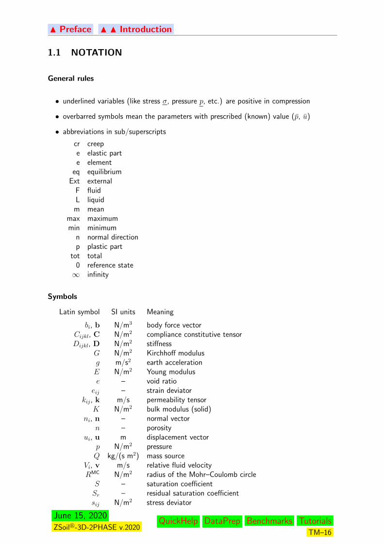
1.1 NOTATION
General rules
• underlined variables (like stress σ, pressure p, etc.) are positive in compression
• overbarred symbols mean the parameters with prescribed (known) value (p, u)
• abbreviations in sub/superscripts
cr creepe elastic parte element
eq equilibriumExt external
F fluidL liquid
m meanmax maximummin minimum
n normal directionp plastic part
tot total0 reference state∞ infinity
Symbols
Latin symbol SI units Meaning
bi, b N/m3 body force vectorCijkl, C N/m2 compliance constitutive tensorDijkl, D N/m2 stiffness
G N/m2 Kirchhoff modulusg m/s2 earth accelerationE N/m2 Young moduluse – void ratioeij – strain deviator
kij, k m/s permeability tensorK N/m2 bulk modulus (solid)
ni, n – normal vectorn – porosity
ui, u m displacement vectorp N/m2 pressureQ kg/(s m2) mass source
Vi, v m/s relative fluid velocityRMC N/m2 radius of the Mohr–Coulomb circleS – saturation coefficientSr – residual saturation coefficientsij N/m2 stress deviator
June 15, 2020ZSoilr-3D-2PHASE v.2020
QuickHelp DataPrep Benchmarks TutorialsTM–16

N Preface N N Introduction
Greek symbol SI units Meaning
εij, ε – strain tensorη Ns/m2 fluid viscosityγ N/m3 specific weight
Γ = ∂Ω m boundary of the domain ΩΓp m boundary with imposed pressure conditionsΓq m boundary with imposed flow conditionsΓs m boundary with imposed seepage (i.e. pressure dependent) flow conditionsΓt m boundary with imposed traction conditionsΓu m boundary with imposed displacement conditionsλ N/m2 Lame constantν – Poisson coefficientρ kg/m3 mass density
σij, σ N/m2 stress tensorσ′ij, σ
′ N/m2 effective stress tensorτ ij, σ N/m2 shear stress tensor
June 15, 2020ZSoilr-3D-2PHASE v.2020
QuickHelp DataPrep Benchmarks TutorialsTM–17

N Preface N N Introduction
1.2 SOME IMPORTANT FORMULAE IN TENSOR ALGEBRA ANDANALYSIS
In mechanics several tensorial variables of different rank are used. Examples are:
scalar (zeroth rank tensor) — density ρ, temperature T , energy W , . . .
vector (first rank tensor)— displacement vector u, velocity vector v, . . .
dyad (second rank tensor) — stress tensor σ, deformation tensor ε , . . .
— fourth, sixth and higher rank tensor — material tensor . . .
Some rules of calculations with tensors in the three-dimensional Euclidean space are presentedin this section. The direct (symbolic) and the component notation of tensor quantities areused. For shorter writing we introduce the Einstein’s summation convention (repeated indexin some term in the expression requires summation)
. . .+ aibi + . . . = · · ·+3∑i=1
aibi + . . . = . . .+ a1b1 + a2b2 + a3b3 + . . .
i is a dummy index.
June 15, 2020ZSoilr-3D-2PHASE v.2020
QuickHelp DataPrep Benchmarks TutorialsTM–18
N Preface N N Introduction
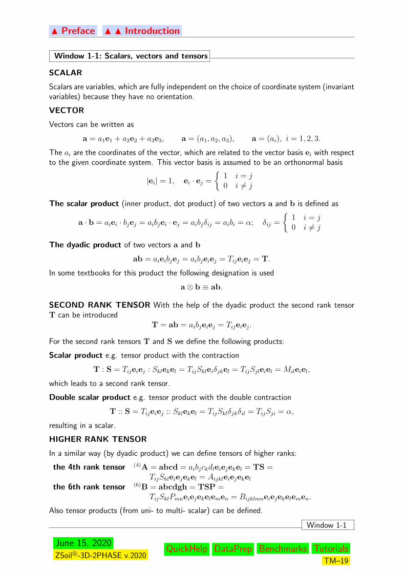
Window 1-1: Scalars, vectors and tensors
SCALAR
Scalars are variables, which are fully independent on the choice of coordinate system (invariantvariables) because they have no orientation.
VECTOR
Vectors can be written as
a = a1e1 + a2e2 + a3e3, a = (a1, a2, a3), a = (ai), i = 1, 2, 3.
The ai are the coordinates of the vector, which are related to the vector basis ei with respectto the given coordinate system. This vector basis is assumed to be an orthonormal basis
|ei| = 1, ei · ej =
1 i = j0 i 6= j
The scalar product (inner product, dot product) of two vectors a and b is defined as
a · b = aiei · bjej = aibjei · ej = aibjδij = aibi = α; δij =
1 i = j0 i 6= j
The dyadic product of two vectors a and b
ab = aieibjej = aibjeiej = Tijeiej = T.
In some textbooks for this product the following designation is used
a⊗ b ≡ ab.
SECOND RANK TENSOR With the help of the dyadic product the second rank tensorT can be introduced
T = ab = aibjeiej = Tijeiej.
For the second rank tensors T and S we define the following products:
Scalar product e.g. tensor product with the contraction
T : S = Tijeiej : Sklekel = TijSkleiδjkel = TijSjleiel = Mileiel,
which leads to a second rank tensor.
Double scalar product e.g. tensor product with the double contraction
T :: S = Tijeiej :: Sklekel = TijSklδjkδil = TijSji = α,
resulting in a scalar.
HIGHER RANK TENSOR
In a similar way (by dyadic product) we can define tensors of higher ranks:
the 4th rank tensor (4)A = abcd = aibjckdleiejekel = TS =TijSkleiejekel = Aijkleiejekel
the 6th rank tensor (6)B = abcdgh = TSP =TijSklPmneiejekelemen = Bijklmneiejekelemen.
Also tensor products (from uni- to multi- scalar) can be defined.
Window 1-1
June 15, 2020ZSoilr-3D-2PHASE v.2020
QuickHelp DataPrep Benchmarks TutorialsTM–19
N Preface N N Introduction
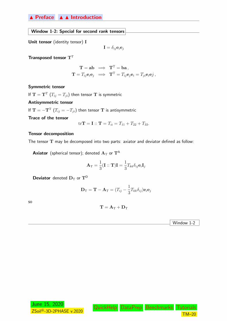
Window 1-2: Special for second rank tensors
Unit tensor (identity tensor) II = δijeiej
Transposed tensor TT
T = ab =⇒ TT = ba ,
T = Tijeiej =⇒ TT = Tijejei = Tjieiej ,
Symmetric tensor
If T = TT (Tij = Tji) then tensor T is symmetric
Antisymmetric tensor
If T = −TT (Tij = −Tji) then tensor T is antisymmetric
Trace of the tensortrT = I :: T = Tii = T11 + T22 + T33.
Tensor decomposition
The tensor T may be decomposed into two parts: axiator and deviator defined as follow:
Axiator (spherical tensor); denoted AT or TA
AT =1
3(I :: T)I =
1
3TkkδijeiIj
Deviator denoted DT or TD
DT = T−AT = (Tij −1
3Tkkδij)eiej
soT = AT + DT
Window 1-2
June 15, 2020ZSoilr-3D-2PHASE v.2020
QuickHelp DataPrep Benchmarks TutorialsTM–20
N Preface N N Introduction
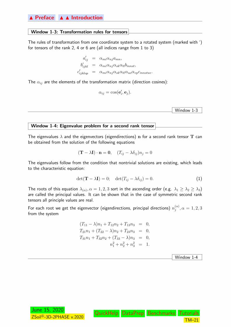
Window 1-3: Transformation rules for tensors
The rules of transformation from one coordinate system to a rotated system (marked with ‘)for tensors of the rank 2, 4 or 6 are (all indices range from 1 to 3)
a′ij = αmiαnjamn,
b′ijkl = αmiαnjαskαtlbmnst,
c′ijklop = αmiαnjαskαtlαuoαvpcmnstuv.
The αij are the elements of the transformation matrix (direction cosines):
αij = cos(e′i, ej).
Window 1-3
Window 1-4: Eigenvalue problem for a second rank tensor
The eigenvalues λ and the eigenvectors (eigendirections) n for a second rank tensor T canbe obtained from the solution of the following equations
(T− λI) · n = 0, (Tij − λδij)nj = 0
The eigenvalues follow from the condition that nontrivial solutions are existing, which leadsto the characteristic equation:
det(T− λI) = 0; det(Tij − λδij) = 0. (1)
The roots of this equation λ(α), α = 1, 2, 3 sort in the ascending order (e.g. λ1 ≥ λ2 ≥ λ3)are called the principal values. It can be shown that in the case of symmetric second ranktensors all principle values are real.
For each root we get the eigenvector (eigendirections, principal directions) n(α)j , α = 1, 2, 3
from the system
(T11 − λ)n1 + T12n2 + T13n3 = 0,
T21n1 + (T22 − λ)n2 + T23n3 = 0,
T31n1 + T32n2 + (T33 − λ)n3 = 0,
n21 + n2
2 + n23 = 1.
Window 1-4
June 15, 2020ZSoilr-3D-2PHASE v.2020
QuickHelp DataPrep Benchmarks TutorialsTM–21
N Preface N N Introduction
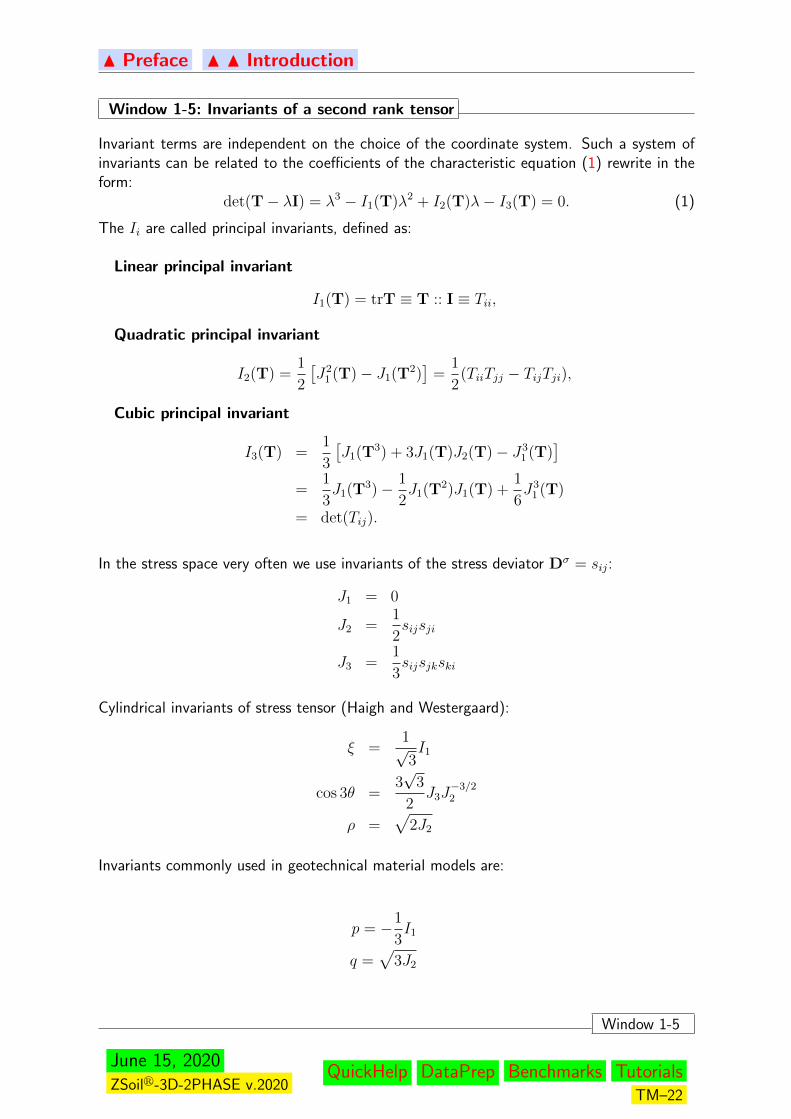
Window 1-5: Invariants of a second rank tensor
Invariant terms are independent on the choice of the coordinate system. Such a system ofinvariants can be related to the coefficients of the characteristic equation (1) rewrite in theform:
det(T− λI) = λ3 − I1(T)λ2 + I2(T)λ− I3(T) = 0. (1)
The Ii are called principal invariants, defined as:
Linear principal invariant
I1(T) = trT ≡ T :: I ≡ Tii,
Quadratic principal invariant
I2(T) =1
2
[J2
1 (T)− J1(T2)]
=1
2(TiiTjj − TijTji),
Cubic principal invariant
I3(T) =1
3
[J1(T3) + 3J1(T)J2(T)− J3
1 (T)]
=1
3J1(T3)− 1
2J1(T2)J1(T) +
1
6J3
1 (T)
= det(Tij).
In the stress space very often we use invariants of the stress deviator Dσ = sij:
J1 = 0
J2 =1
2sijsji
J3 =1
3sijsjkski
Cylindrical invariants of stress tensor (Haigh and Westergaard):
ξ =1√3I1
cos 3θ =3√
3
2J3J
−3/22
ρ =√
2J2
Invariants commonly used in geotechnical material models are:
p = −1
3I1
q =√
3J2
Window 1-5
June 15, 2020ZSoilr-3D-2PHASE v.2020
QuickHelp DataPrep Benchmarks TutorialsTM–22

N Preface N N Introduction
Window 1-6: Cayley-Hamilton theorem
The second rank tensor satisfies characteristic equation
T3 − I1(T)T2 + I2(T)T− I3(T)I = 0,
which enables the representation of Tn (n ≥ 3) as a linear function of T2,T,T0 = I, e.g.,
T3 = I1(T)T2 − I2(T)T + I3(T)I.
Window 1-6
Window 1-7: Derivatives of the invariants of a second rank tensor
A scalar-valued function of a second rank tensor can be represented by
ψ = ψ(T) = ψ(T11, T22, . . . , T31).
Then we can calculate the derivative by the following equation
ψ,T =∂ψ
∂T=
∂ψ
∂Tklekel.
On the other hand the derivatives of the invariants are
J1(T),T = I, J1(T2),T = 2TT, J1(T3),T = 3T2T,
J2(T),T = J1(T)I−TT,
J3(T),T = T2T − J1(T)TT + J2(T)I = J3(T)(TT)−1.
So, we finally get
ψ[J1, J2, J3],T =
(∂ψ
∂J1
+ J1∂ψ
∂J2
+ J2∂ψ
∂J3
)I−
(∂ψ
∂J2
+ J1∂ψ
∂J3
)TT +
∂ψ
∂J3
T2T.
These calculations can be helpful for the use of the representation theorem of an isotropicfunction
P = F(T) = ν0I + ν1T + ν2T2.
The coefficients νi itself are functions of the invariants
νi = νi [J1(T), J2(T), J3(T)] . (1)
Window 1-7
June 15, 2020ZSoilr-3D-2PHASE v.2020
QuickHelp DataPrep Benchmarks TutorialsTM–23

N Preface N N Introduction
Window 1-8: Transition from tensorial to matrix notation
It is assumed that stress/strain components are ordered in column vectors as follows:
σ =σxx σyy τxy σzz τxz τ yz
T
ε =εxx εyy γxy εzz γxz γyz
T
The following table is used to extract vector components from appropriate tensorial objects:
I/J i/k j/l1 1 12 2 23 1 24 3 35 1 36 2 3
With the above table we can set:
- I-th component of stress vector σ : σI = σi(I)j(I)
- I-th component of strain vector ε : εI = εi(I)j(I) (shear terms have to doubled)
- I-th, J-th component of stiffness matrix D : DIJ = Di(I)j(I)k(J)l(J)
Window 1-8
June 15, 2020ZSoilr-3D-2PHASE v.2020
QuickHelp DataPrep Benchmarks TutorialsTM–24
N Preface N N Introduction
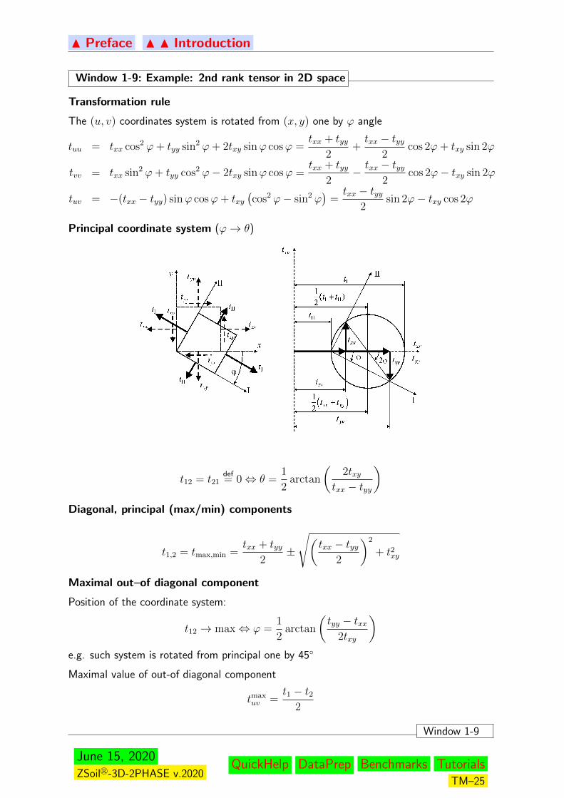
Window 1-9: Example: 2nd rank tensor in 2D space
Transformation rule
The (u, v) coordinates system is rotated from (x, y) one by ϕ angle
tuu = txx cos2 ϕ+ tyy sin2 ϕ+ 2txy sinϕ cosϕ =txx + tyy
2+txx − tyy
2cos 2ϕ+ txy sin 2ϕ
tvv = txx sin2 ϕ+ tyy cos2 ϕ− 2txy sinϕ cosϕ =txx + tyy
2− txx − tyy
2cos 2ϕ− txy sin 2ϕ
tuv = −(txx − tyy) sinϕ cosϕ+ txy(cos2 ϕ− sin2 ϕ
)=txx − tyy
2sin 2ϕ− txy cos 2ϕ
Principal coordinate system (ϕ→ θ)
t12 = t21def= 0⇔ θ =
1
2arctan
(2txy
txx − tyy
)Diagonal, principal (max/min) components
t1,2 = tmax,min =txx + tyy
2±
√(txx − tyy
2
)2
+ t2xy
Maximal out–of diagonal component
Position of the coordinate system:
t12 → max⇔ ϕ =1
2arctan
(tyy − txx
2txy
)e.g. such system is rotated from principal one by 45
Maximal value of out-of diagonal component
tmaxuv =
t1 − t22
Window 1-9
June 15, 2020ZSoilr-3D-2PHASE v.2020
QuickHelp DataPrep Benchmarks TutorialsTM–25

N Preface N N Introduction
June 15, 2020ZSoilr-3D-2PHASE v.2020
QuickHelp DataPrep Benchmarks TutorialsTM–26

N Preface
Chapter 2
PROBLEM STATEMENT
In following sections formulations of problems available to be solved are given. In particular:
SINGLE PHASE
TWO PHASE
TRANSIENT FLOW
HEAT TRANSFER
HUMIDITY TRANSFER
They contain governing differential equations and boundary conditions (strong formulation).Despite this, for each problem variational formulations (weak form) are given which are thebasis for numerical solution.
June 15, 2020ZSoilr-3D-2PHASE v.2020
QuickHelp DataPrep Benchmarks TutorialsTM–27
N Preface N N Problem Statement
2.1 SINGLE PHASE, SOLID MEDIUM
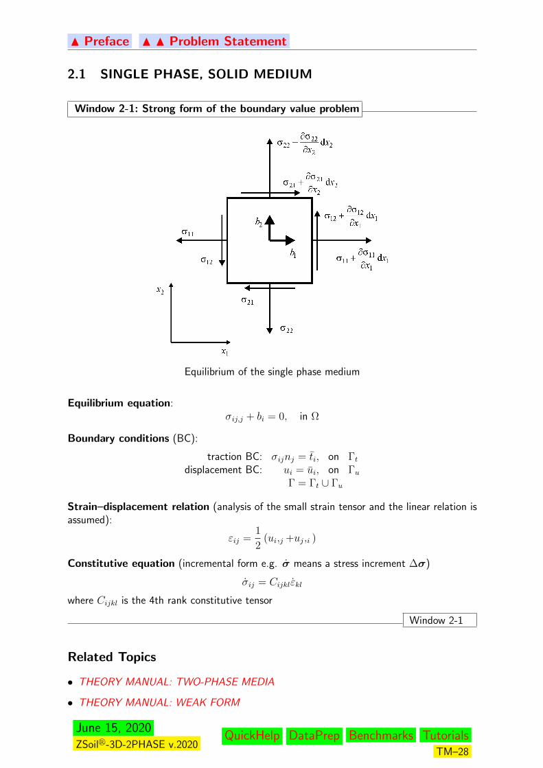
Window 2-1: Strong form of the boundary value problem
Equilibrium of the single phase medium
Equilibrium equation:σij,j + bi = 0, in Ω
Boundary conditions (BC):
traction BC: σijnj = ti, on Γtdisplacement BC: ui = ui, on Γu
Γ = Γt ∪ Γu
Strain–displacement relation (analysis of the small strain tensor and the linear relation isassumed):
εij =1
2(ui,j +uj,i )
Constitutive equation (incremental form e.g. σ means a stress increment ∆σ)
σij = Cijklεkl
where Cijkl is the 4th rank constitutive tensor
Window 2-1
Related Topics
• THEORY MANUAL: TWO-PHASE MEDIA
• THEORY MANUAL: WEAK FORM
June 15, 2020ZSoilr-3D-2PHASE v.2020
QuickHelp DataPrep Benchmarks TutorialsTM–28
N Preface N N Problem Statement
2.2 TWO-PHASE PARTIALLY SATURATED MEDIUM
The simulation of a two–phase medium is necessary in order to account for time-dependentbehaviour resulting from consolidation and/or transient flow. Actual creep will be discussedlater on.
The boundary–value–problem to be solved requires the coupled solution of conservation ofmass and momentum in both the solid and the liquid phases, together with boundary andinitial conditions. The general transient case is considered here.
The Windows in section present:
Two phase medium model – Window 2-2
Equilibrium of two phase medium – Window 2-3
Strong form of BVP for two phase partially saturated medium – Window 2-4
Strong form of BVP for two phase fully saturated medium – Window 2-5
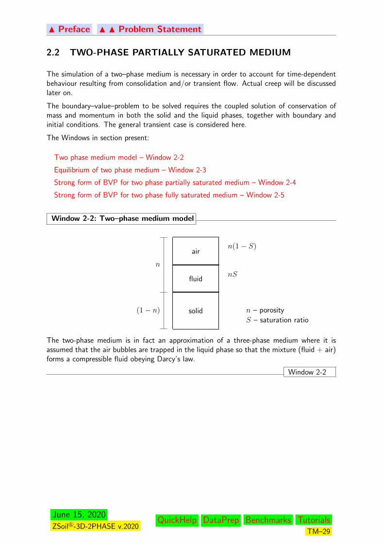
Window 2-2: Two–phase medium model
(1− n)
n
nS
n(1− S)
n – porosity
S – saturation ratiosolid
fluid
air
The two-phase medium is in fact an approximation of a three-phase medium where it isassumed that the air bubbles are trapped in the liquid phase so that the mixture (fluid + air)forms a compressible fluid obeying Darcy’s law.
Window 2-2
June 15, 2020ZSoilr-3D-2PHASE v.2020
QuickHelp DataPrep Benchmarks TutorialsTM–29
N Preface N N Problem Statement
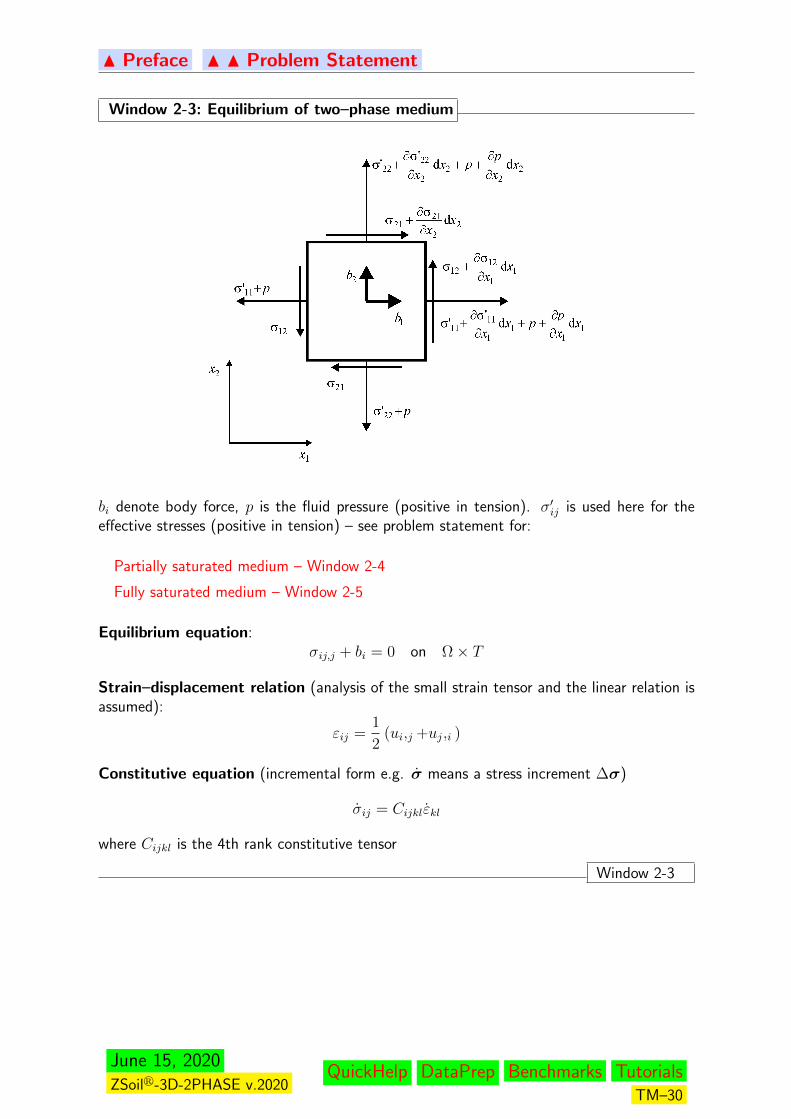
Window 2-3: Equilibrium of two–phase medium
bi denote body force, p is the fluid pressure (positive in tension). σ′ij is used here for theeffective stresses (positive in tension) – see problem statement for:
Partially saturated medium – Window 2-4
Fully saturated medium – Window 2-5
Equilibrium equation:σij,j + bi = 0 on Ω× T
Strain–displacement relation (analysis of the small strain tensor and the linear relation isassumed):
εij =1
2(ui,j +uj,i )
Constitutive equation (incremental form e.g. σ means a stress increment ∆σ)
σij = Cijklεkl
where Cijkl is the 4th rank constitutive tensor
Window 2-3
June 15, 2020ZSoilr-3D-2PHASE v.2020
QuickHelp DataPrep Benchmarks TutorialsTM–30
N Preface N N Problem Statement
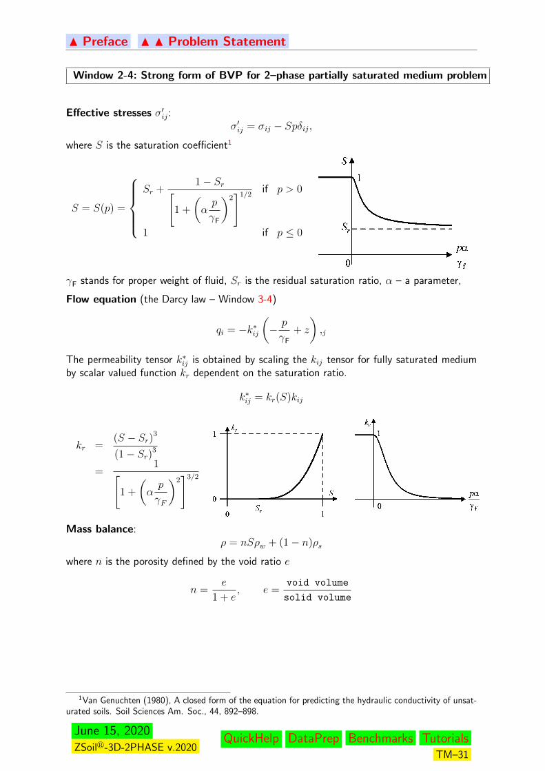
Window 2-4: Strong form of BVP for 2–phase partially saturated medium problem
Effective stresses σ′ij:σ′ij = σij − Spδij,
where S is the saturation coefficient1
S = S(p) =
Sr +
1− Sr[1 +
(αp
γF
)2]1/2
if p > 0
1 if p ≤ 0
γF stands for proper weight of fluid, Sr is the residual saturation ratio, α – a parameter,
Flow equation (the Darcy law – Window 3-4)
qi = −k∗ij(− p
γF
+ z
),j
The permeability tensor k∗ij is obtained by scaling the kij tensor for fully saturated mediumby scalar valued function kr dependent on the saturation ratio.
k∗ij = kr(S)kij
kr =(S − Sr)3
(1− Sr)3
=1[
1 +
(αp
γF
)2]3/2
Mass balance:ρ = nSρw + (1− n)ρs
where n is the porosity defined by the void ratio e
n =e
1 + e, e =
void volume
solid volume
1Van Genuchten (1980), A closed form of the equation for predicting the hydraulic conductivity of unsat-urated soils. Soil Sciences Am. Soc., 44, 892–898.
June 15, 2020ZSoilr-3D-2PHASE v.2020
QuickHelp DataPrep Benchmarks TutorialsTM–31
N Preface N N Problem Statement
Continuity equation:Sεkk + qk,k = cp
with c the specific storage coefficient
c = c(p) = n
(S
KF+
dS
dp
)KF – fluid bulk modulus
Boundary conditions:
on solid phase on fluid phase
σijnj = ti on Γtui = ui on Γu,
qjnj = q on Γqqjnj = qs on Γs
p = p on ΓpΓ = Γu + Γt Γ = Γp + Γq + Γs
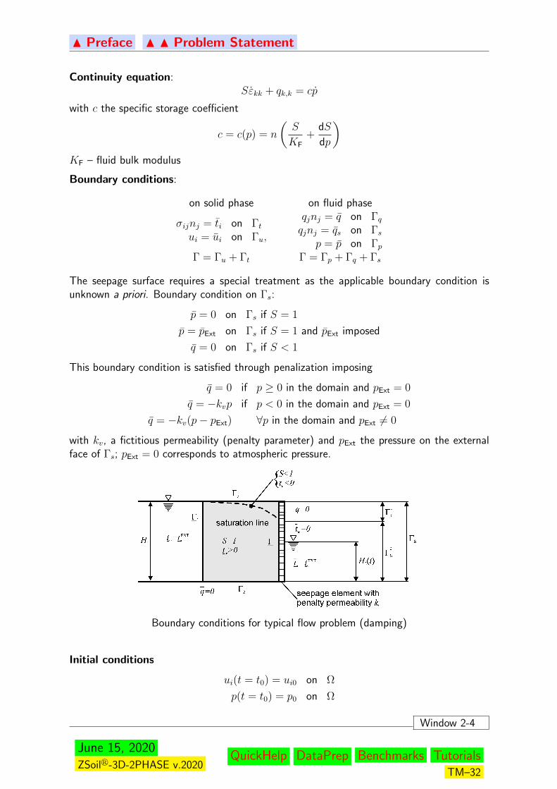
The seepage surface requires a special treatment as the applicable boundary condition isunknown a priori. Boundary condition on Γs:
p = 0 on Γs if S = 1
p = pExt on Γs if S = 1 and pExt imposed
q = 0 on Γs if S < 1
This boundary condition is satisfied through penalization imposing
q = 0 if p ≥ 0 in the domain and pExt = 0
q = −kvp if p < 0 in the domain and pExt = 0
q = −kv(p− pExt) ∀p in the domain and pExt 6= 0
with kv, a fictitious permeability (penalty parameter) and pExt the pressure on the externalface of Γs; pExt = 0 corresponds to atmospheric pressure.
Boundary conditions for typical flow problem (damping)
Initial conditions
ui(t = t0) = ui0 on Ω
p(t = t0) = p0 on Ω
Window 2-4
June 15, 2020ZSoilr-3D-2PHASE v.2020
QuickHelp DataPrep Benchmarks TutorialsTM–32
N Preface N N Problem Statement
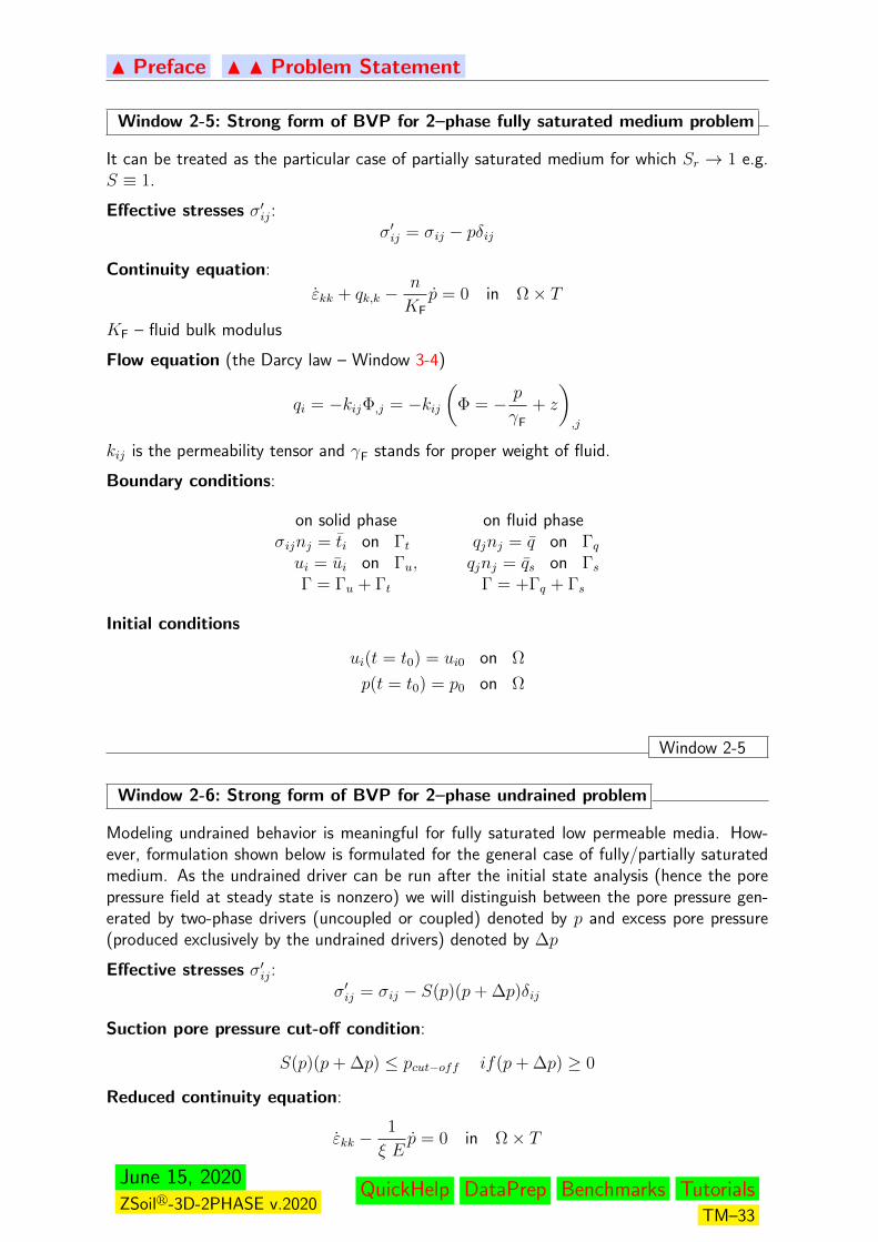
Window 2-5: Strong form of BVP for 2–phase fully saturated medium problem
It can be treated as the particular case of partially saturated medium for which Sr → 1 e.g.S ≡ 1.
Effective stresses σ′ij:σ′ij = σij − pδij
Continuity equation:
εkk + qk,k −n
KFp = 0 in Ω× T
KF – fluid bulk modulus
Flow equation (the Darcy law – Window 3-4)
qi = −kijΦ,j = −kij(
Φ = − p
γF
+ z
),j
kij is the permeability tensor and γF stands for proper weight of fluid.
Boundary conditions:
on solid phase on fluid phaseσijnj = ti on Γtui = ui on Γu,
qjnj = q on Γqqjnj = qs on Γs
Γ = Γu + Γt Γ = +Γq + Γs
Initial conditions
ui(t = t0) = ui0 on Ω
p(t = t0) = p0 on Ω
Window 2-5
Window 2-6: Strong form of BVP for 2–phase undrained problem
Modeling undrained behavior is meaningful for fully saturated low permeable media. How-ever, formulation shown below is formulated for the general case of fully/partially saturatedmedium. As the undrained driver can be run after the initial state analysis (hence the porepressure field at steady state is nonzero) we will distinguish between the pore pressure gen-erated by two-phase drivers (uncoupled or coupled) denoted by p and excess pore pressure(produced exclusively by the undrained drivers) denoted by ∆p
Effective stresses σ′ij:σ′ij = σij − S(p)(p+ ∆p)δij
Suction pore pressure cut-off condition:
S(p)(p+ ∆p) ≤ pcut−off if(p+ ∆p) ≥ 0
Reduced continuity equation:
εkk −1
ξ Ep = 0 in Ω× T
June 15, 2020ZSoilr-3D-2PHASE v.2020
QuickHelp DataPrep Benchmarks TutorialsTM–33

N Preface N N Problem Statement
E – solid elastic Young’s modulusξ – penalty factor (106 ÷ 108)
Boundary conditions: To be set as for single-phase problems
Window 2-6
Related Topics
• THEORY MANUAL: TRANSIENT FLOW
• THEORY MANUAL: SINGLE PHASE, SOLID MEDIUM
• THEORY MANUAL: TWO–PHASE MEDIA. APPROXIMATION AND MATRIX FORM
• THEORY MANUAL: TWO–PHASE MEDIA. WEAK FORM
June 15, 2020ZSoilr-3D-2PHASE v.2020
QuickHelp DataPrep Benchmarks TutorialsTM–34

N Preface N N Problem Statement
2.3 TRANSIENT FLOW
Transient flow problem formulation may be derived from two–phase media formulation, seesection 2.2. The only primary state variable is pore pressures p. In continuity equation, termresulting from skeleton volume changes εkk should be neglected. Constitutive relation for theflow (generalized Darcy law will take identical form). Also boundary contitions for fluid phaseare identical as in the case of two–phase media.
June 15, 2020ZSoilr-3D-2PHASE v.2020
QuickHelp DataPrep Benchmarks TutorialsTM–35
N Preface N N Problem Statement
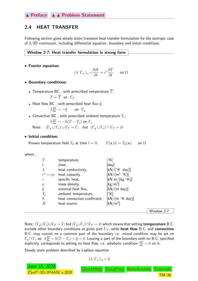
2.4 HEAT TRANSFER
Following section gives steady state/transient heat transfer formulation for the isotropic caseof 2/3D continuum, including differential equation, boundary and initial conditions.
Window 2-7: Heat transfer formulation in strong form
• Fourier equation:
(λ T,i ),i +∂H
∂t= c∗
∂T
∂ton Ω
• Boundary conditions:
F Temperature BC , with prescribed temperature T :
T = T on ΓT
F Heat flow BC , with prescribed heat flux q:
λ∂T∂n
= −q on Γq
F Convective BC , with prescribed ambient temperature Te:
λ∂T∂n
= −h(T − Te) on Γc
Note: (Γq ∪ Γc) ∪ ΓT = Γ; but (Γq ∪ Γc) ∩ ΓT = ∅
• Initial condition:
Known temperature field T0 at time t = 0: T (x,0) = T0(x) on Ω
where :
T temperature, [K]t time, [day]λ heat conductivity, [kN/(K day)]c∗ = cρ heat capacity, [kN/(m2 K)]c specific heat, [kN m/(kg K)]ρ mass density, [kg/m3]q external heat flux, [kN/(m day)]Te ambient temperature, [K]h heat convection coefficient, [kN/(m K day)]H heat source [kN/m2]
Window 2-7
Note: (Γq∪Γc)∪ΓT = Γ; but (Γq∪Γc)∩ΓT = ∅ which means that setting temperature B.C.exclude other boundary conditions at given part ΓT , while heat flow B.C. and convectiveB.C. may coexist on a common part of the boundary i.e. mixed condition may be set onΓq ∩Γc as: λ∂T
∂n+ h(T − Te) + q = 0. Leaving a part of the boundary with no B.C. specified
explicitly, corresponds to setting no heat flow, i.e. adiabatic condition ∂T∂n
= 0 on it.
Steady state problem described by Laplace equation
(λ T,i ),i = 0
June 15, 2020ZSoilr-3D-2PHASE v.2020
QuickHelp DataPrep Benchmarks TutorialsTM–36

N Preface N N Problem Statement
can be formulated. Physically, it describes continuum at thermal equilibrium state, whilemathematically it corresponds to a limit of the transient problem at time t → ∞ with allstate variables independent from time.
It is possible to define λ(T ) and c∗(T ) as explicit functions of temperature.
The source term H adopted in the formulation is related to the phenomena of heat emissionduring concrete hydration process and is described by the following set of equations:
Window 2-8: Concrete hydration heat source
• heat source as a function of maturity M :
H(t, T ) = H∞(aM)b
1 + (aM)b
• maturity M as a function of absolute temperature T and time t:
M(t, T ) =
t∫td
exp
[Q
R
(1
Tf− 1
T
)]dt
where:
H∞ total value of concrete hydration heat per unit volume [kJ/m3],a heat source parameter [1/day]b heat source parameter [-]Q/R activation energy/universal gas constant [K]Tf reference temperature, normally 20C = 293K [K]td dormant period [day]
Window 2-8
June 15, 2020ZSoilr-3D-2PHASE v.2020
QuickHelp DataPrep Benchmarks TutorialsTM–37
N Preface N N Problem Statement
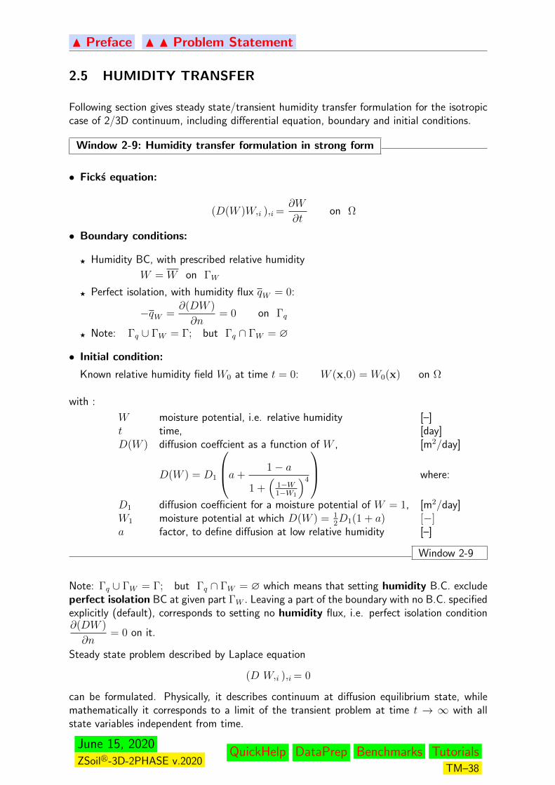
2.5 HUMIDITY TRANSFER
Following section gives steady state/transient humidity transfer formulation for the isotropiccase of 2/3D continuum, including differential equation, boundary and initial conditions.
Window 2-9: Humidity transfer formulation in strong form
• Ficks equation:
(D(W )W,i ),i =∂W
∂ton Ω
• Boundary conditions:
F Humidity BC, with prescribed relative humidity
W = W on ΓW
F Perfect isolation, with humidity flux qW = 0:
−qW =∂(DW )
∂n= 0 on Γq
F Note: Γq ∪ ΓW = Γ; but Γq ∩ ΓW = ∅
• Initial condition:
Known relative humidity field W0 at time t = 0: W (x,0) = W0(x) on Ω
with :
W moisture potential, i.e. relative humidity [–]t time, [day]D(W ) diffusion coeffcient as a function of W , [m2/day]
D(W ) = D1
a+1− a
1 +(
1−W1−W1
)4
where:
D1 diffusion coefficient for a moisture potential of W = 1, [m2/day]W1 moisture potential at which D(W ) = 1
2D1(1 + a) [−]
a factor, to define diffusion at low relative humidity [–]
Window 2-9
Note: Γq ∪ ΓW = Γ; but Γq ∩ ΓW = ∅ which means that setting humidity B.C. excludeperfect isolation BC at given part ΓW . Leaving a part of the boundary with no B.C. specifiedexplicitly (default), corresponds to setting no humidity flux, i.e. perfect isolation condition∂(DW )
∂n= 0 on it.
Steady state problem described by Laplace equation
(D W,i ),i = 0
can be formulated. Physically, it describes continuum at diffusion equilibrium state, whilemathematically it corresponds to a limit of the transient problem at time t → ∞ with allstate variables independent from time.
June 15, 2020ZSoilr-3D-2PHASE v.2020
QuickHelp DataPrep Benchmarks TutorialsTM–38

N Preface
Chapter 3
MATERIAL MODELS
ELASTICITY
CREEP
CONSOLIDATION
PLASTICITY
SWELLING
AGING CONCRETE
APPENDICES
June 15, 2020ZSoilr-3D-2PHASE v.2020
QuickHelp DataPrep Benchmarks TutorialsTM–39
N Preface N N Material Models
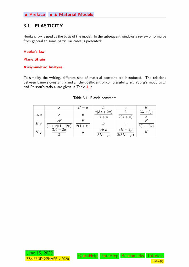
3.1 ELASTICITY
Hooke’s law is used as the basis of the model. In the subsequent windows a review of formulaefrom general to some particular cases is presented:
Hooke’s law
Plane Strain
Axisymmetric Analysis
To simplify the writing, different sets of material constant are introduced. The relationsbetween Lame’s constant λ and µ, the coefficient of compressibility K, Young’s modulus Eand Poisson’s ratio ν are given in Table 3.1:
Table 3.1: Elastic constants
λ G = µ E ν K
λ, µ λ µµ(3λ+ 2µ)
λ+ µ
λ
2(λ+ µ)
3λ+ 2µ
3
E, ννE
(1 + ν)(1− 2ν)
E
2(1 + νE ν
E
3(1− 2ν)
K,µ3K − 2µ
3µ
9Kµ
3K + µ
3K − 2µ
2(3K + µ)K
June 15, 2020ZSoilr-3D-2PHASE v.2020
QuickHelp DataPrep Benchmarks TutorialsTM–40
N Preface N N Material Models
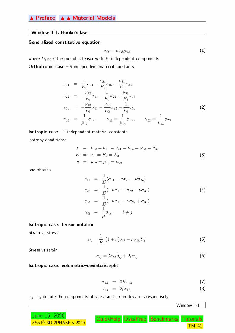
Window 3-1: Hooke’s law
Generalized constitutive equation
σij = Dijklεkl (1)
where Dijkl is the modulus tensor with 36 independent components
Orthotropic case – 9 independent material constants
ε11 =1
E1
σ11 −ν21
E2
σ22 −ν31
E3
σ33
ε22 = −ν12
E1
σ11 −1
E2
σ22 −ν32
E3
σ33
ε33 = −ν13
E1
σ11 −ν23
E2
σ22 −1
E3
σ33 (2)
γ12 =1
µ12
σ12 , γ13 =1
µ13
σ13 , γ23 =1
µ23
σ23
Isotropic case – 2 independent material constants
Isotropy conditions:
ν = ν12 = ν21 = ν31 = ν13 = ν23 = ν32
E = E1 = E2 = E3 (3)
µ = µ12 = µ13 = µ23
one obtains:
ε11 =1
E(σ11 − νσ22 − νσ33)
ε22 =1
E(−νσ11 + σ22 − νσ33) (4)
ε33 =1
E(−νσ11 − νσ22 + σ33)
γij =1
µσij, i 6= j
Isotropic case: tensor notation
Strain vs stress
εij =1
E[(1 + ν)σij − νσkkδij] (5)
Stress vs strainσij = λεkkδij + 2µεij (6)
Isotropic case: volumetric–deviatoric split
σkk = 3Kεkk (7)
sij = 2µeij (8)
sij, eij denote the components of stress and strain deviators respectively
Window 3-1
June 15, 2020ZSoilr-3D-2PHASE v.2020
QuickHelp DataPrep Benchmarks TutorialsTM–41
N Preface N N Material Models
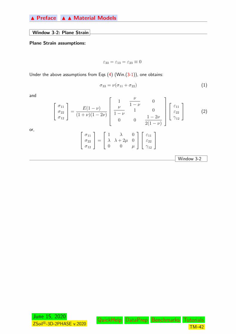
Window 3-2: Plane Strain
Plane Strain assumptions:
ε33 = ε13 = ε23 ≡ 0
Under the above assumptions from Eqs (4) (Win.(3-1)), one obtains:
σ33 = ν(σ11 + σ22) (1)
and σ11
σ22
σ12
=E(1− ν)
(1 + ν)(1− 2ν)
1
ν
1− ν0
ν
1− ν1 0
0 01− 2ν
2(1− ν)
ε11
ε22
γ12
(2)
or, σ11
σ22
σ12
=
1 λ 0λ λ+ 2µ 00 0 µ
ε11
ε22
γ12
Window 3-2
June 15, 2020ZSoilr-3D-2PHASE v.2020
QuickHelp DataPrep Benchmarks TutorialsTM–42
N Preface N N Material Models
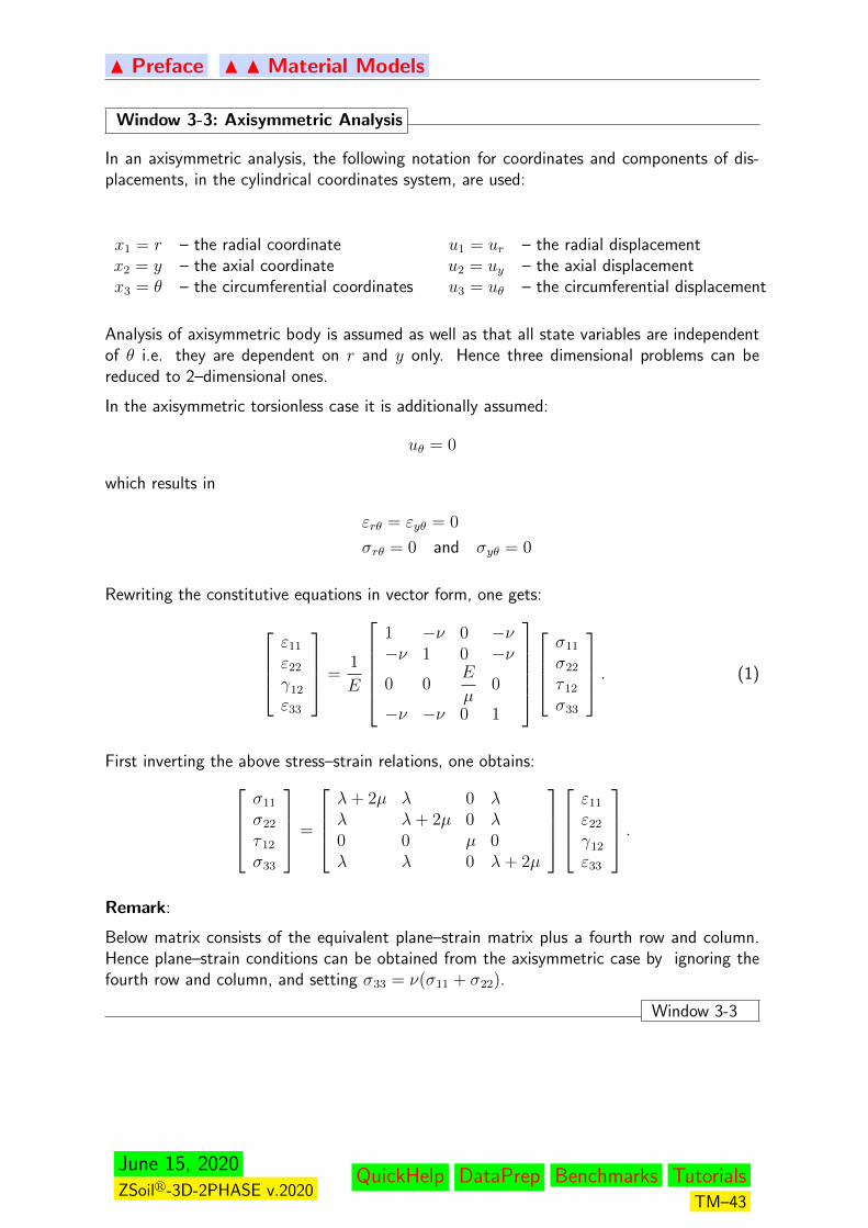
Window 3-3: Axisymmetric Analysis
In an axisymmetric analysis, the following notation for coordinates and components of dis-placements, in the cylindrical coordinates system, are used:
x1 = r – the radial coordinate u1 = ur – the radial displacementx2 = y – the axial coordinate u2 = uy – the axial displacementx3 = θ – the circumferential coordinates u3 = uθ – the circumferential displacement
Analysis of axisymmetric body is assumed as well as that all state variables are independentof θ i.e. they are dependent on r and y only. Hence three dimensional problems can bereduced to 2–dimensional ones.
In the axisymmetric torsionless case it is additionally assumed:
uθ = 0
which results in
εrθ = εyθ = 0
σrθ = 0 and σyθ = 0
Rewriting the constitutive equations in vector form, one gets:
ε11
ε22
γ12
ε33
=1
E
1 −ν 0 −ν−ν 1 0 −ν
0 0E
µ0
−ν −ν 0 1
σ11
σ22
τ 12
σ33
. (1)
First inverting the above stress–strain relations, one obtains:σ11
σ22
τ 12
σ33
=
λ+ 2µ λ 0 λλ λ+ 2µ 0 λ0 0 µ 0λ λ 0 λ+ 2µ
ε11
ε22
γ12
ε33
.Remark:
Below matrix consists of the equivalent plane–strain matrix plus a fourth row and column.Hence plane–strain conditions can be obtained from the axisymmetric case by ignoring thefourth row and column, and setting σ33 = ν(σ11 + σ22).
Window 3-3
June 15, 2020ZSoilr-3D-2PHASE v.2020
QuickHelp DataPrep Benchmarks TutorialsTM–43

N Preface N N Material Models
3.2 CONSOLIDATION
Primary consolidation is discussed in this section.
It results from the coupling of load–induced Darcy flow with the motion of a quasi–saturatedmedium.
DARCY LAW
FLUID MOTION
Related Topics
• THEORY: TWO PHASE MEDIA
• NUMERICAL IMPLEMENTATION: CONSOLIDATION
• GEOTECHNICAL ASPECTS: TWO PHASE MEDIA
June 15, 2020ZSoilr-3D-2PHASE v.2020
QuickHelp DataPrep Benchmarks TutorialsTM–44
N Preface N N Material Models N N Consolidation
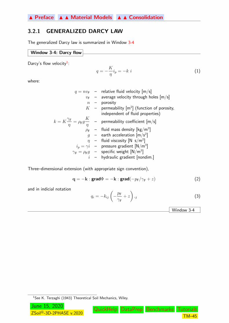
3.2.1 GENERALIZED DARCY LAW
The generalized Darcy law is summarized in Window 3-4
Window 3-4: Darcy flow
Darcy’s flow velocity1:
q = −Kηip = −k i (1)
where:
q = nvF – relative fluid velocity [m/s]vF – average velocity through holes [m/s]n – porosityK – permeability [m2] (function of porosity,
independent of fluid properties)
k = KγF
η= ρFg
K
η– permeability coefficient [m/s]
ρF – fluid mass density [kg/m3]g – earth acceleration [m/s2]η – fluid viscosity [N s/m2]
ip = γi – pressure gradient [N/m3]γF = ρFg – specific weight [N/m3]
i – hydraulic gradient [nondim.]
Three–dimensional extension (with appropriate sign convention),
q = −k : gradΦ = −k : grad(−pF/γF + z) (2)
and in indicial notation
qi = −kij(−pF
γF
+ z
),j (3)
Window 3-4
1See K. Terzaghi (1943) Theoretical Soil Mechanics, Wiley.
June 15, 2020ZSoilr-3D-2PHASE v.2020
QuickHelp DataPrep Benchmarks TutorialsTM–45
N Preface N N Material Models N N Consolidation
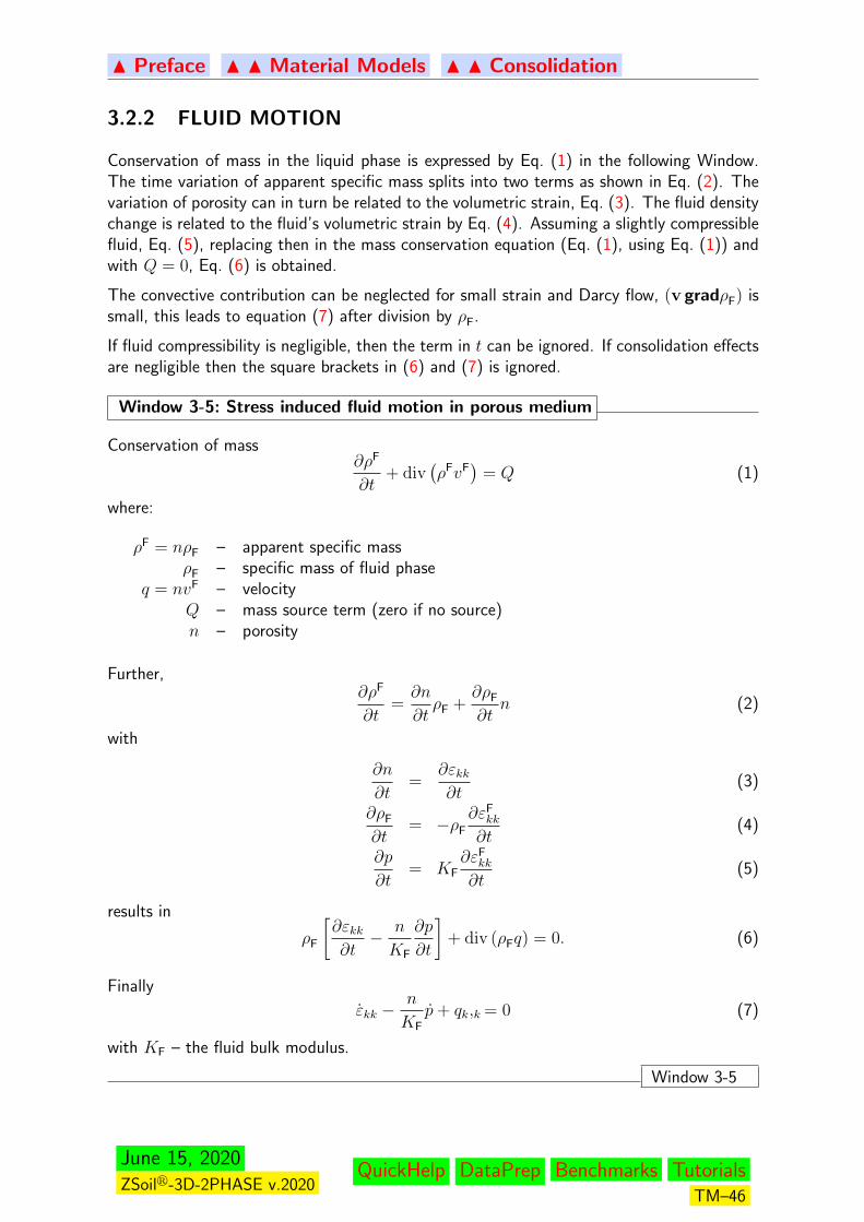
3.2.2 FLUID MOTION
Conservation of mass in the liquid phase is expressed by Eq. (1) in the following Window.The time variation of apparent specific mass splits into two terms as shown in Eq. (2). Thevariation of porosity can in turn be related to the volumetric strain, Eq. (3). The fluid densitychange is related to the fluid’s volumetric strain by Eq. (4). Assuming a slightly compressiblefluid, Eq. (5), replacing then in the mass conservation equation (Eq. (1), using Eq. (1)) andwith Q = 0, Eq. (6) is obtained.
The convective contribution can be neglected for small strain and Darcy flow, (v gradρF) issmall, this leads to equation (7) after division by ρF.
If fluid compressibility is negligible, then the term in t can be ignored. If consolidation effectsare negligible then the square brackets in (6) and (7) is ignored.
Window 3-5: Stress induced fluid motion in porous medium
Conservation of mass∂ρF
∂t+ div
(ρFvF
)= Q (1)
where:
ρF = nρF – apparent specific massρF – specific mass of fluid phase
q = nvF – velocityQ – mass source term (zero if no source)n – porosity
Further,∂ρF
∂t=∂n
∂tρF +
∂ρF
∂tn (2)
with
∂n
∂t=
∂εkk∂t
(3)
∂ρF
∂t= −ρF
∂εFkk
∂t(4)
∂p
∂t= KF
∂εFkk
∂t(5)
results in
ρF
[∂εkk∂t− n
KF
∂p
∂t
]+ div (ρFq) = 0. (6)
Finally
εkk −n
KFp+ qk,k = 0 (7)
with KF – the fluid bulk modulus.
Window 3-5
June 15, 2020ZSoilr-3D-2PHASE v.2020
QuickHelp DataPrep Benchmarks TutorialsTM–46

N Preface N N Material Models
3.3 PLASTICITY
SKETCH OF PLASTICITY APPROACH
MOHR–COULOMB CRITERION
DRUCKER–PRAGER CRITERION
CAP MODEL
CAM-CLAY MODEL
June 15, 2020ZSoilr-3D-2PHASE v.2020
QuickHelp DataPrep Benchmarks TutorialsTM–47

N Preface N N Material Models N N N Plasticity
3.3.1 SKETCH OF THE PLASTICITY APPROACH
Plasticity is a nonlinear constitutive theory and leads to a nonlinear system of equations, whichis solved iteratively for ∆d, the displacement increment, using a tangent (local) stiffness.Once the displacement increment is known the corresponding strain increment results fromthe usual strain–displacement relations. From the strain increment a trial stress can bededuced which, if it lies outside of the yield criterion, must be returned onto the criterionusing a flow rule. This flow rule defines the direction of the stress return. The amplitude ofthe return results from the consistency condition, which requires the new state–of–stress tolie on the yield criterion. The objective, in this section, is to define precisely the new keywordsintroduced for plasticity theory. The basic ingredients of the elasto–plasticity theory are asfollows:
Strain decomposition
Assume that the total strain increment (or rate) is the sum of an elastic εe and a plastic εp
contribution:ε = εe + εp
and that the following constitutive equation holds:
σ = De(ε− εp)
with De the elastic constitutive tensor.
Flow rule
The flow rule defines the direction of the plastic flow by:
εp = dλ r(σ,q)
where dλ is a positive scalar which defines the amplitude of the plastic flow and r (in generala function of the stress state σ and set of a hardening parameters q) defines the direction inspace. The calculation of dλ will be described later on.
For associative plasticity the direction of the flow r coincides with that of the normal a tothe yield surface:
a = r =∂F
∂σ
while for non–associative plasticity, we assume the existence of a plastic potential surface Qsuch that:
r =∂Q
∂σ
Hardening law
The most general form of hardening law can be expressed in rate form as follows:
q = dλ h(σ,q)
where h (in general a function of the stress state σ and of a set of hardening parameters q)is called hardening function.
June 15, 2020ZSoilr-3D-2PHASE v.2020
QuickHelp DataPrep Benchmarks TutorialsTM–48
N Preface N N Material Models N N N Plasticity
The amplitude of the plastic flow
The amplitude of plastic flow can be derived from the consistency condition, which expressesthat the stress point remains on the yield surface during plastic flow:
F =∂F
∂σ: σ +
∂F
∂q: q = a : De : (ε− εp) +
∂F
∂q: q
= a : De : (ε− dλ r) +∂F
∂q: dλ h = 0.
From the above equation, in which the flow rule and the hardening rule have been applied,the amplitude dλ can be evaluated:
dλ =(a : De : ε)
(a : De : r)−∂F∂q
: h
Derivation of the elasto–plastic tangent matrix
Applying the amplitude dλ to the general constitutive equation the tangent elasto–plasticconstitutive matrix is defined in the following way:
σ = De : (ε− εp) = De : (ε− dλ r) = De :
ε− r(a : De : ε)
(a : De : r)−∂F∂q
: h
=
De − De : r : a : De
(a : De : r)−∂F∂q
: h
ε = Depε
In case of perfect elasto–plasticity (no hardening is introduced) the definition of the tangentmatrix reduces to:
Dep = De − De : r : a : De
(a : De : r).
For a nonassociative plastic flow rule the resulting tangent matrix is nonsymmetric.
June 15, 2020ZSoilr-3D-2PHASE v.2020
QuickHelp DataPrep Benchmarks TutorialsTM–49

N Preface N N Material Models N N N Plasticity
3.3.2 MOHR–COULOMB CRITERION
The Mohr–Coulomb (M–C) criterion is more common in soil mechanics. Traditionally, a soilis described by its cohesion C and its angle of friction φ. The M–C criterion then statesthat the shear stress required for yielding depends on the cohesion, the friction angle and thepressure normal to the slip surface.
Window 3-6: Mohr-Coulomb yield criterion
Mohr-Coulomb yield criterion
| τ |= c+ σn tanφ (1)
where
ρ =σ11 + σ22
2(2)
and,RMC = c cosφ+ ρ sinφ (3)
is the maximum shear stress equal to radius of the Mohr circle at failure, i.e.:
RMC =
√(σ11 − σ22)2
4+ τ 2
12 (4)
Window 3-6
June 15, 2020ZSoilr-3D-2PHASE v.2020
QuickHelp DataPrep Benchmarks TutorialsTM–50

N Preface N N Material Models N N N Plasticity
3.3.3 DRUCKER-PRAGER CRITERION
The Drucker–Prager (D–P) yield criterion is, mathematically speaking, the most convenientchoice and often numerically the most efficient. The D–P criterion is defined in stress space,by the following equation:
F (σ) =aφI1 +√J2 − k = 0
where the invariants I1 and J2 are defined in Section 1.2 and aφ and k are positive materialproperties. For aφ = 0, Huber–Mises criterion results.
Flow rule
Associative plasticity: the direction of the flow r coincides with that of the normal a to theyield surface:
a = r =∂F
∂σ= aφδij +
1
2√J2
sij
Non–associative plasticity: the existence of a plastic potential surface Q of Drucker–Pragertype is assumed:
rij =∂Q
∂σij= aψδij +
1
2√J2
sij
Notice that the corresponding flow is associative in the deviatoric component and non–associative in the volumetric components, as aψ = aφ.
Cut-off condition
The following tensile cutt–off plasticity condition can be activated in conjunction with theDrucker–Prager plasticity criterion:
F (σ) =1√3I1 +
√J2 −
1√3I ′1T = 0.
It has two basic features, first that maximum first stress invariant I1 is limited to the valueI ′1T for zero deviatoric stress s and the second that the maximum stress ratio defined as:
q
p= −3
√3J2
I1
≤ 3
is limited to the value which can be reached in the uniaxial compression test.
The flow rule has been assumed as fully associated so the plastic flow vector r is:
rij =∂F
∂σij=
1√3δij +
1
2√J2
sij.
Matching of Drucker–Prager criterion
Drucker–Prager constants could be derived directly from experiments, instead of calculatedfrom cohesion and friction angle. Assuming that the material is properly identified by aMohr–Coulomb criterion, the matching with the Drucker–Prager criterion can be done forvarious stress states.
Three dimensional matching
Collapse load matching
Elastic domains matching
June 15, 2020ZSoilr-3D-2PHASE v.2020
QuickHelp DataPrep Benchmarks TutorialsTM–51
N Preface N N Material Models N N N Plasticity
Window 3-7: D–P criterion: Three dimensional matching
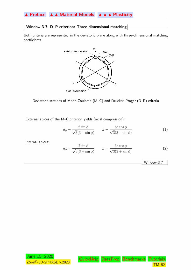
Both criteria are represented in the deviatoric plane along with three–dimensional matchingcoefficients.
Deviatoric sections of Mohr–Coulomb (M–C) and Drucker–Prager (D–P) criteria
External apices of the M–C criterion yields (axial compression):
aφ =2 sinφ√
3(3− sinφ)k =
6c cosφ√3(3− sinφ)
(1)
Internal apices:
aφ =2 sinφ√
3(3 + sinφ)k =
6c cosφ√3(3 + sinφ)
(2)
Window 3-7
June 15, 2020ZSoilr-3D-2PHASE v.2020
QuickHelp DataPrep Benchmarks TutorialsTM–52
N Preface N N Material Models N N N Plasticity
Window 3-8: Matching of collapse load (plane strain conditions)
Matching collapse load of D–P and M-C criteria under plane strain conditions is the defaultadjustment adopted in the program when plane strain is activated.
Assumptions:
perfect plasticity: εe εp ⇒ εe = 0; ε = εp (1)
plane strain: εp33 = εp13 = εp23 = 0 (2)
flow rule : εpij = dλ rij = dλ
(aψδij +
1
2√J2
sij
), (3)
rij =∂Q
∂σij
From (3)
s33 = −2aψ√J2; s13 = s23 = 0
and invariants
I1 =3
2(σ11 + σ22)− 3aψ
√J2 ; J2 =
[(σ11 − σ22) /2]2 + σ2
12
(1− 3a2
ψ)=
(RMC)2
(1− 3a2ψ)
From D–P criterion (F (σ) =aφI1 +√J2 − k = 0):
3
2aφ(σ11 + σ22) +
RMC(1− 3aφaψ)√(1− 3a2
ψ)− k = 0 (4)
one obtains
RMC =
√(1− 3a2
ψ)
(1− 3aφaψ)
[−3aφ(σ11 + σ22)
2+ k
](5)
Identification with Mohr–Coulomb criterion, Eq. 4
sinφ = 3aφ
√(1− 3a2
ψ)
(1− 3aφaψ), c cosφ = k
√(1− 3a2
ψ)
(1− 3aφaψ)(6)
Associated flow aψ = aφ
aφ =tanφ√
9 + 12 tan2 φ, k =
3c√9 + 12 tan2 φ
(7)
Deviatoric flow aψ = 0
aφ =sinφ
3, k = c cosφ (8)
aψ specified:
aφ =sinφ
3
(aψ sinφ+
√1− 3a2
ψ
)−1
, k = c cosφ(aψ sinφ+
√1− 3a2
ψ
)−1
(9)
Window 3-8
June 15, 2020ZSoilr-3D-2PHASE v.2020
QuickHelp DataPrep Benchmarks TutorialsTM–53
N Preface N N Material Models N N N Plasticity
Window 3-9: Matching of elastic domain
Plane strain conditions are assumed.
D–P criterion (square form of F (σ) =aφI1 +√J2 − k = 0):
a2φI
21 − 2aφI1k + k2 = J2 (1)
and invariants:
I1 = (σ11 + σ22)(1 + ν)
J2 =1
3
[(σ11 − σ22)2 (1− ν + ν2) + σ11σ22(1− 2ν)2
]+ σ2
12
(D–P) :
(σ11 − σ22
2
)2
+ σ212 = k2 − 2aφk(1 + ν)(σ11 + σ22)
+(σ11 + σ22)2
[a2φ(1 + ν)2 − 1
12(1− 2ν)2
](M–C) :
(σ11 − σ22
2
)2
+ σ212 = c2 cos2 φ− 2
σ11 + σ22
2sinφ c cosφ
+
(σ11 + σ22
2
)2
sin2 φ
Matching the constant, linear and quadratic terms (σ11 + σ22) yields:
aφ =sinφ
2(1 + ν)
k = c cosφ
ν = 0.5
i.e. stress–state–independent matching is possible for arbitrary c and φ only when ν = 0.5.Alternatively, when c = 0, matching is possible for arbitrary φ for a specified ν.
Window 3-9
June 15, 2020ZSoilr-3D-2PHASE v.2020
QuickHelp DataPrep Benchmarks TutorialsTM–54
N Preface N N Material Models N N N Plasticity
3.3.4 CAP MODEL
While the constitutive models described previously could be applied to any kind of material,the following one is more specific to soils.
Model is describe in the subsequent windows:
Yield surface
It combines the Drucker–Prager criterion with an ellipsoidal cap closure analogous to theCAM–CLAY ellipse and the tensile cutt–off defined in Section 3.3.3 (if needed). Multisur-face plasticity algorithms require the cap definition to be extended to the zone which iscovered by the D–P criterion (that is for p < p
cs) where it takes the form of a cylinder. p
cdenotes the preconsolidation pressure defines the current cap size.
Flow rule
Associative flow is assumed on the cap; the corresponding flow vector is derived in Win.(3-10).
Hardening law
The hardening law defines the evolution of the size of the cap yield surface. This requiresthe evolution law for p
cas a function of plastic strain. The corresponding derivation
is given in Window 3-11, where Eqs (2) and (3) define respectively the total and theelastic contributions in (4); Eq.( 5) results which relates the hardening parameter p
cto the
volumetric plastic strain
Remark:
Underlined variables are positive in compression.
June 15, 2020ZSoilr-3D-2PHASE v.2020
QuickHelp DataPrep Benchmarks TutorialsTM–55
N Preface N N Material Models N N N Plasticity
Window 3-10: Cap model: Yield surface and plastic flow vectors
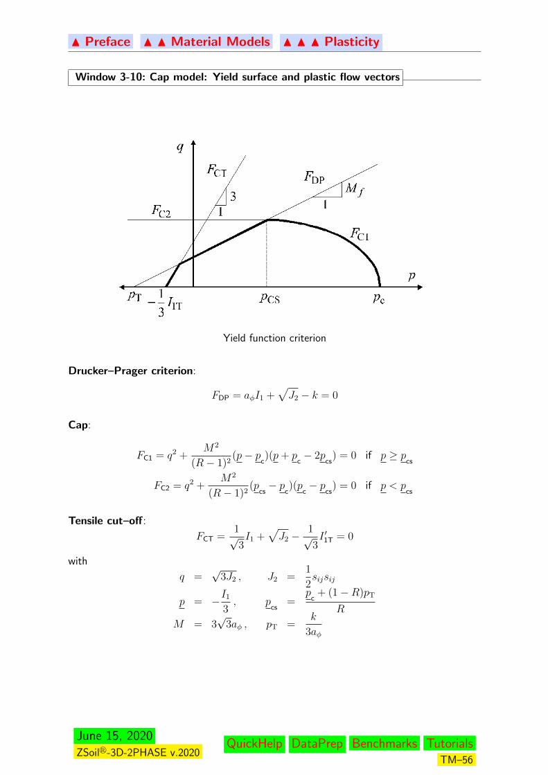
Yield function criterion
Drucker–Prager criterion:
FDP = aφI1 +√J2 − k = 0
Cap:
FC1 = q2 +M2
(R− 1)2(p− p
c)(p+ p
c− 2p
cs) = 0 if p ≥ p
cs
FC2 = q2 +M2
(R− 1)2(p
cs− p
c)(p
c− p
cs) = 0 if p < p
cs
Tensile cut–off:
FCT =1√3I1 +
√J2 −
1√3I ′1T = 0
with
q =√
3J2 , J2 =1
2sijsij
p = −I1
3, p
cs=
pc
+ (1−R)pT
R
M = 3√
3aφ , pT =k
3aφ
June 15, 2020ZSoilr-3D-2PHASE v.2020
QuickHelp DataPrep Benchmarks TutorialsTM–56
N Preface N N Material Models N N N Plasticity
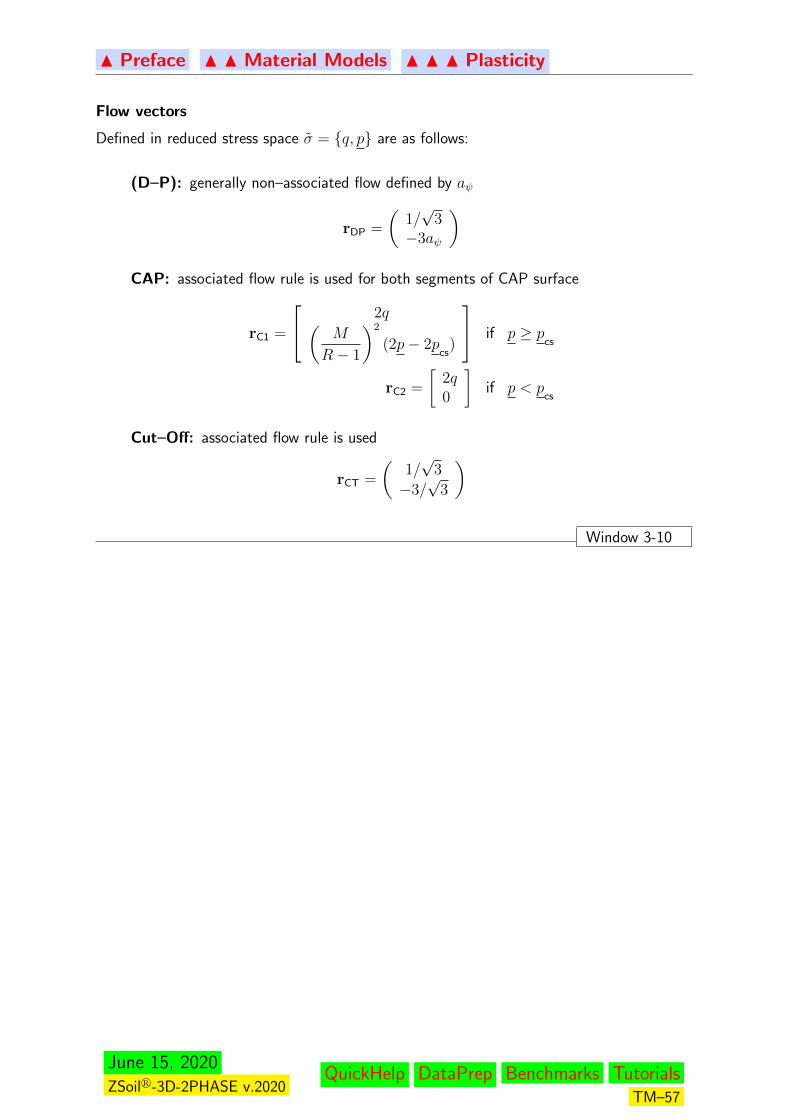
Flow vectors
Defined in reduced stress space σ = q, p are as follows:
(D–P): generally non–associated flow defined by aψ
rDP =
(1/√
3−3aψ
)CAP: associated flow rule is used for both segments of CAP surface
rC1 =
2q(M
R− 1
)2
(2p− 2pcs
)
if p ≥ pcs
rC2 =
[2q0
]if p < p
cs
Cut–Off: associated flow rule is used
rCT =
(1/√
3
−3/√
3
)
Window 3-10
June 15, 2020ZSoilr-3D-2PHASE v.2020
QuickHelp DataPrep Benchmarks TutorialsTM–57
N Preface N N Material Models N N N Plasticity
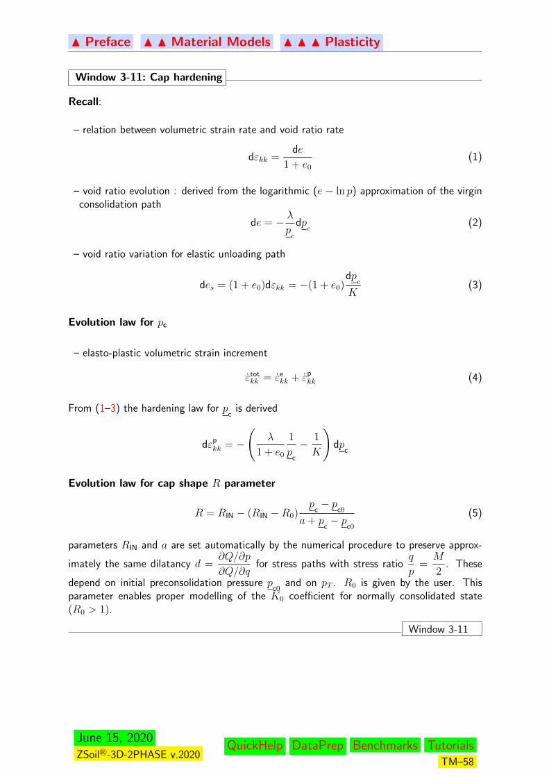
Window 3-11: Cap hardening
Recall:
– relation between volumetric strain rate and void ratio rate
dεkk =de
1 + e0
(1)
– void ratio evolution : derived from the logarithmic (e− ln p) approximation of the virginconsolidation path
de = − λpc
dpc
(2)
– void ratio variation for elastic unloading path
des = (1 + e0)dεkk = −(1 + e0)dp
c
K(3)
Evolution law for pc
– elasto-plastic volumetric strain increment
εtotkk = εe
kk + εpkk (4)
From (1–3) the hardening law for pc
is derived
dεpkk = −
(λ
1 + e0
1
pc
− 1
K
)dp
c
Evolution law for cap shape R parameter
R = RIN − (RIN −R0)p
c− p
c0
a+ pc− p
c0
(5)
parameters RIN and a are set automatically by the numerical procedure to preserve approx-
imately the same dilatancy d =∂Q/∂p
∂Q/∂qfor stress paths with stress ratio
q
p=M
2. These
depend on initial preconsolidation pressure pc0
and on pT . R0 is given by the user. Thisparameter enables proper modelling of the K0 coefficient for normally consolidated state(R0 > 1).
Window 3-11
June 15, 2020ZSoilr-3D-2PHASE v.2020
QuickHelp DataPrep Benchmarks TutorialsTM–58
N Preface N N Material Models N N N Plasticity
Window 3-12: Evaluation of pco, Ro from oedometer test
The initial preconsolidation stress pco and cap shape parameter Ro can be set based onoedometer test once σVM (vertical stress at which transition from secondary to primaryconsolidation path occurs) and KNC
o (Ko coefficient at state of normal consolidation) valuesare given (see Window 3-13).
In the oedometer test the following relation holds (assuming that plastic strains are largecompared to elastic ones):
dεpV =3
2dεpD
where: dεpD =
√2
3depijde
pij, dε
pV = −dεpii.
This equation can be rewritten in the form (using plastic flow rule and effect of hardening):
1
Hn2p dp+
1
Hnpnq dq =
3
2
(1
Hnqnq dq +
1
Hnqnp dp
)where: np =
∂QC1
∂p(QC1 = FC1− elliptic cap surface)
nq =∂QC1
∂q
dq/dp = ηKo (along Ko path)
H = −∂FC1
∂pc
∂pc
∂εpVnp (plastic modulus for constant shape ratio parameter R)
ηKo =3 (1−KNC
o )
2 KNCo + 1
Window 3-12
Window 3-13: Procedure of evaluation of pco, Ro from oedometer test
Given material properties: eo, E, ν, λ, φ, DP-size adjustment (ak, aφ)
σVM (vertical stress at the transition point from secondary to primary consolidation line),KNCo (Ko at state of normal consolidation)
Find: pco, Ro
• initialize:
i = 0: pT =ak3aφ
, M = 3√
3aφ p(i=0)co =
2 KNCo + 1
3σVM
• next iteration: i = i+ 1• find Ro (see Window 3-14) (for pT = 0)• find modified shape ratio parameter RIN for real value of pT and p(i)
co(see Window 3-15)
• find corrected p(i+1)co
value (see Window 3-16)
• iterate until | p(i+1)co− p(i)
co|> 10−8
Window 3-13
June 15, 2020ZSoilr-3D-2PHASE v.2020
QuickHelp DataPrep Benchmarks TutorialsTM–59

N Preface N N Material Models N N N Plasticity
Window 3-14: Ro evaluation
Given: M, pco, ηKo = q/p (at Ko path) =
3 (1−KNCo )
2 KNCo + 1
Find: Ro (using bisection method)
• Initialize i = 0:
R(i=0)o = 1.01; ∆R = 10−3
• Step i = i+ 1:
R(i)o = R
(i−1)o + ∆R
for given: M , R(i)o , p
co, ηKo compute mean stress p at the intersection point of elliptic
cap surface FC1 and Ko line
compute corresponding deviatoric stress: q = ηKop and np, nq,∂FC1
∂pc
compute residuum of the governing equation for oedometer test: fKo = np/nq −3
2;
• if i > 1 then
if f lastKo∗ fKo ≤ 0 then
set: R(i+1)o = (R
(i)o −∆Ro/2) and EXIT
else
save: f lastKo= fKo and go to next iteration
end if
end if
Window 3-14
June 15, 2020ZSoilr-3D-2PHASE v.2020
QuickHelp DataPrep Benchmarks TutorialsTM–60
N Preface N N Material Models N N N Plasticity
Window 3-15: RIN evaluation
Given: pco
Find: modified shape ratio parameter RIN such that dilatancy parameter d = np/nq isthe same along trial stress path ηM = M/2 (some arbitrary path) both for elliptic cap with
pT = 0 and cap surface with real pT value.
• Initialize i = 0:
Compute dilatancy parameter do = np/nq for given: pco, pT = 0, ηM and shape ratioparameter Ro
set: ∆RIN = 0.01
set: Rlast = Ro
• Step i = i+ 1
R(i)IN = R
(i−1)IN + ∆R
for given M , pco, pT , ηM and shape ratio parameter R = R(i)IN compute compute mean
stress p at the intersection point of elliptic cap surface FC1 and stress path line q/p = ηM
compute corresponding deviatoric stress: q = ηKop and np, nq
compute dilatancy parameter d = np/nq
• if i > 1 then
if do > dlast AND do < d OR do > d AND do < dlast then
set: R(i+1)IN = R
(i)IN +
dlast − dodlast − d
∆RIN and EXIT
else
set: dlast = d and go to next iteration
end if
end if
Window 3-15
Window 3-16: Evaluation of corrected p(i+1)co
value
Given: M , RIN , pT , ν, σVM
Find: p(i+1)co
• Set: Kelo =
ν
1− ν, ηKo
el =3(1−Kel
o )
1 + 2Kelo
, p =(1 + 2Kel
o )σVM
3, q = ηKo
el p
• For p, q, pT , M solve quadratic equation (elliptic cap equation) FC1 = 0 for unknown
p(i+1)co value
Window 3-16
June 15, 2020ZSoilr-3D-2PHASE v.2020
QuickHelp DataPrep Benchmarks TutorialsTM–61
N Preface N N Material Models N N N Plasticity
3.3.5 MOHR-COULOMB (M-W)
•Yield surface The original M–C criterion (see Window 3-6) which leads to a non–smoothmultisurface plasticity problem, is substituted by its smooth, single–surface approximation,being a particular case of a general 3–parameter criterion developed recently by Mentrey(see Menetrey, Willam: A triaxial failure criterion for concrete and its generalization. ACIStructural Journal 92(3) p.311–318). This criterion takes the form described in Window 3-17.
Window 3-17: Menetrey criterion
.
F (ξ, ρ, θ) = (Afρ)2 +mf [Bf ρ rf (θ, e) + Cf ξ]−Df = 0 (1)
where ξ, ρ, θ are Haigh-Westergaard stress coordinates equal to:
ξ =1√3I1 (2)
cos 3θ =3√
3
2J3J
−3
22 (3)
ρ =√
2J2 (4)
with I1, J2, J3 being the usual stress invariants (1-5)
Function rf = rf (θ, e), 0.5 < e ≤ 1, describes the shape of the surface in deviatoric section
rf (θ, e) =4 (1− e2) cos2 θ + (2e− 1)2
2 (1− e2) cos θ + (2e− 1)[4 (1− e2) cos2 θ + (2e− 1)2 − (1− e2)
]1/2 (5)
Window 3-17
The eccentricity parameter e can be calibrated to fit exactly the Mohr–Coulomb surfaceon both extension and compression meridians which leads to the smooth Mohr–Coulombsurface. All other parameters of the generalized criterion are also expressed in terms of theMohr–Coulomb friction angle φ and cohesion c as shown in Window 3-18.
June 15, 2020ZSoilr-3D-2PHASE v.2020
QuickHelp DataPrep Benchmarks TutorialsTM–62
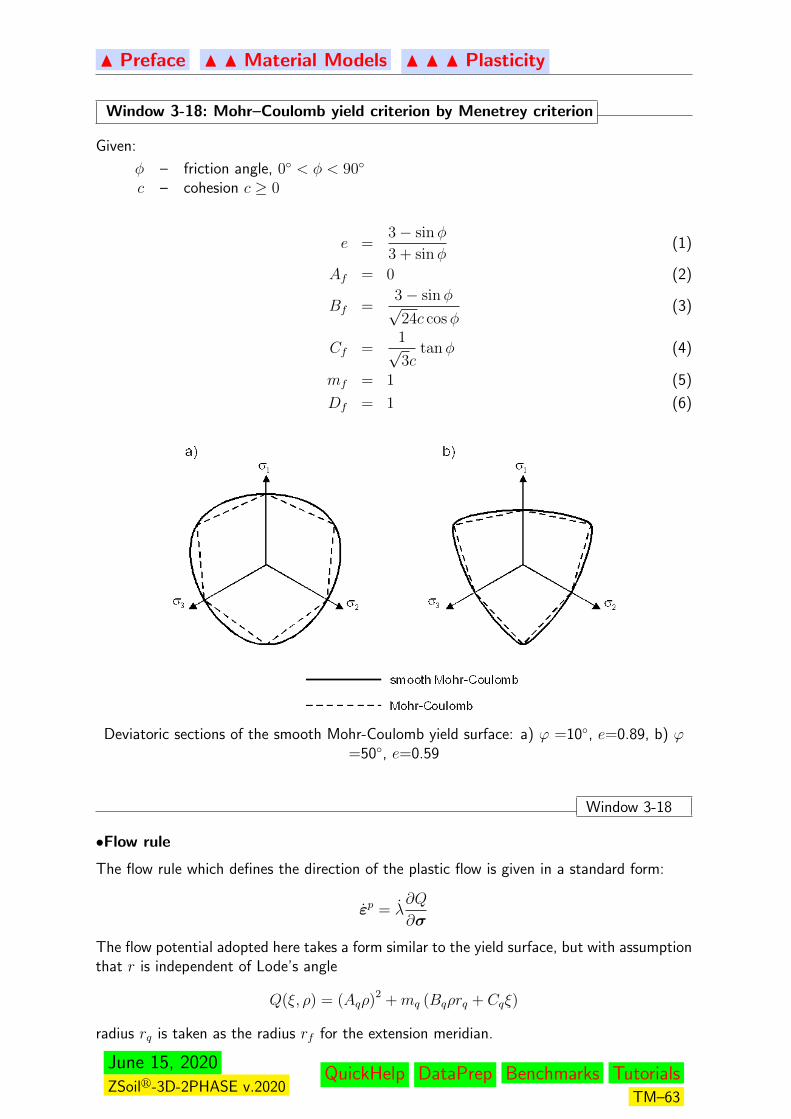
N Preface N N Material Models N N N Plasticity
Window 3-18: Mohr–Coulomb yield criterion by Menetrey criterion
Given:
φ – friction angle, 0 < φ < 90
c – cohesion c ≥ 0
e =3− sinφ
3 + sinφ(1)
Af = 0 (2)
Bf =3− sinφ√24c cosφ
(3)
Cf =1√3c
tanφ (4)
mf = 1 (5)
Df = 1 (6)
Deviatoric sections of the smooth Mohr-Coulomb yield surface: a) ϕ =10, e=0.89, b) ϕ=50, e=0.59
Window 3-18
•Flow rule
The flow rule which defines the direction of the plastic flow is given in a standard form:
εp = λ∂Q
∂σ
The flow potential adopted here takes a form similar to the yield surface, but with assumptionthat r is independent of Lode’s angle
Q(ξ, ρ) = (Aqρ)2 +mq (Bqρrq + Cqξ)
radius rq is taken as the radius rf for the extension meridian.
June 15, 2020ZSoilr-3D-2PHASE v.2020
QuickHelp DataPrep Benchmarks TutorialsTM–63
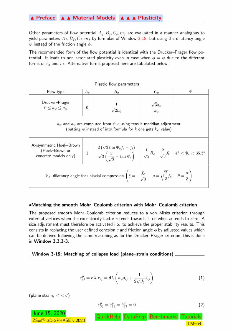
N Preface N N Material Models N N N Plasticity
Other parameters of flow potential Aq, Bq, Cq,mq are evaluated in a manner analogous toyield parameters Af , Bf , Cf ,mf by formulae of Window 3-18, but using the dilatancy angleψ instead of the friction angle φ.
The recommended form of the flow potential is identical with the Drucker–Prager flow po-tential. It leads to non associated plasticity even in case when φ = ψ due to the differentforms of rq and rf . Alternative forms proposed here are tabulated below.
Plastic flow parameters
Flow type Aq Bq Cq Ψ
01√2kψ
√3aψkψ
Drucker–Prager0 ≤ aψ ≤ aφ
kψ and aψ are computed from ψ, c using tensile meridian adjustment(putting ψ instead of into formula for k one gets kψ value)
1
2(√
2 tan Ψcfc − ft)
√3
(1√2− tan Ψc
) 1√2Bq +
2√3ft 4 < Ψc < 35.3
Axisymmetric Hoek–Brown(Hoek–Brown or
concrete models only)
Ψc- dilatancy angle for uniaxial compression
(ξ = − fc√
3, ρ =
√2
3fc, θ =
π
3
)
•Matching the smooth Mohr–Coulomb criterion with Mohr–Coulomb criterion
The proposed smooth Mohr–Coulomb criterion reduces to a von–Mises criterion throughexternal vertices when the excentricity factor e tends towards 1, i.e when φ tends to zero. Asize adjustment must therefore be activated i.o. to achieve the proper stability results. Thisconsists in replacing the user defined cohesion c and friction angle φ by adjusted values whichcan be derived following the same reasoning as for the Drucker–Prager criterion; this is donein Window 3.3.3-3.
Window 3-19: Matching of collapse load (plane–strain conditions)
εpij = dλ rij = dλ
(aψδij +
1
2√J2
sij
)(1)
(plane strain, εe <<)
εp33 = εp13 = εp23 = 0 (2)
June 15, 2020ZSoilr-3D-2PHASE v.2020
QuickHelp DataPrep Benchmarks TutorialsTM–64
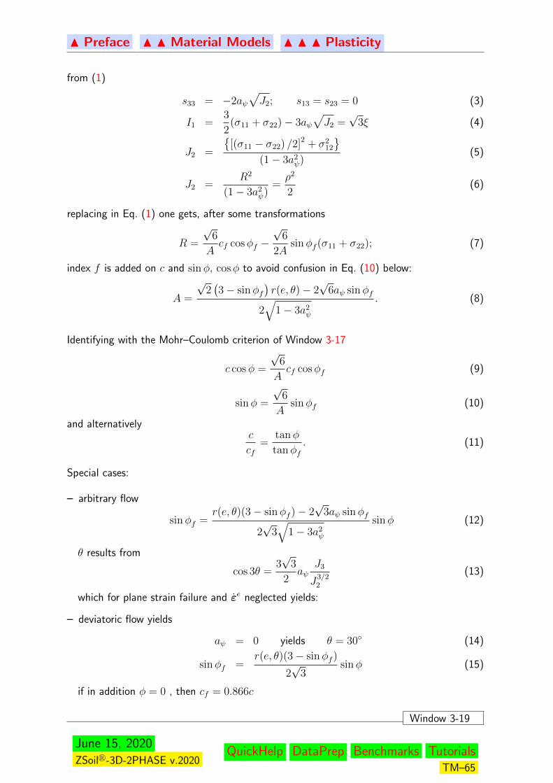
N Preface N N Material Models N N N Plasticity
from (1)
s33 = −2aψ√J2; s13 = s23 = 0 (3)
I1 =3
2(σ11 + σ22)− 3aψ
√J2 =
√3ξ (4)
J2 =
[(σ11 − σ22) /2]2 + σ2
12
(1− 3a2
ψ)(5)
J2 =R2
(1− 3a2ψ)
=ρ2
2(6)
replacing in Eq. (1) one gets, after some transformations
R =
√6
Acf cosφf −
√6
2Asinφf (σ11 + σ22); (7)
index f is added on c and sinφ, cosφ to avoid confusion in Eq. (10) below:
A =
√2(3− sinφf
)r(e, θ)− 2
√6aψ sinφf
2√
1− 3a2ψ
. (8)
Identifying with the Mohr–Coulomb criterion of Window 3-17
c cosφ =
√6
Acf cosφf (9)
sinφ =
√6
Asinφf (10)
and alternativelyc
cf=
tanφ
tanφf. (11)
Special cases:
– arbitrary flow
sinφf =r(e, θ)(3− sinφf )− 2
√3aψ sinφf
2√
3√
1− 3a2ψ
sinφ (12)
θ results from
cos 3θ =3√
3
2aψ
J3
J3/22
(13)
which for plane strain failure and εe neglected yields:
– deviatoric flow yields
aψ = 0 yields θ = 30 (14)
sinφf =r(e, θ)(3− sinφf )
2√
3sinφ (15)
if in addition φ = 0 , then cf = 0.866c
Window 3-19
June 15, 2020ZSoilr-3D-2PHASE v.2020
QuickHelp DataPrep Benchmarks TutorialsTM–65
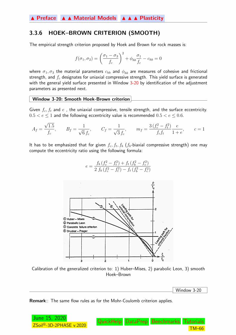
N Preface N N Material Models N N N Plasticity
3.3.6 HOEK–BROWN CRITERION (SMOOTH)
The empirical strength criterion proposed by Hoek and Brown for rock masses is:
f(σ1, σ2) =
(σ1 − σ3
fc
)2
+ φhbσ1
fc− chb = 0
where σ1, σ3 the material parameters chb and φhb are measures of cohesive and frictionalstrength, and fc designates for uniaxial compressive strength. This yield surface is generatedwith the general yield surface presented in Window 3-20 by identification of the adjustmentparameters as presented next.
Window 3-20: Smooth Hoek-Brown criterion
Given fc, ft and e , the uniaxial compressive, tensile strength, and the surface eccentricity.0.5 < e ≤ 1 and the following eccentricity value is recommended 0.5 < e ≤ 0.6.
Af =
√1.5
fc, Bf =
1√6 fc
, Cf =1√3 fc
, mf =3 (f 2
c − f 2t )
fcft
e
1 + e, c = 1
It has to be emphasized that for given fc, ft, fb (fb-biaxial compressive strength) one maycompute the eccentricity ratio using the following formula:
e =fb (f 2
c − f 2t ) + ft (f 2
b − f 2c )
2 fb (f 2c − f 2
t )− ft (f 2b − f 2
c )
Calibration of the generalized criterion to: 1) Huber–Mises, 2) parabolic Leon, 3) smoothHoek–Brown
Window 3-20
Remark:: The same flow rules as for the Mohr-Coulomb criterion applies.
June 15, 2020ZSoilr-3D-2PHASE v.2020
QuickHelp DataPrep Benchmarks TutorialsTM–66
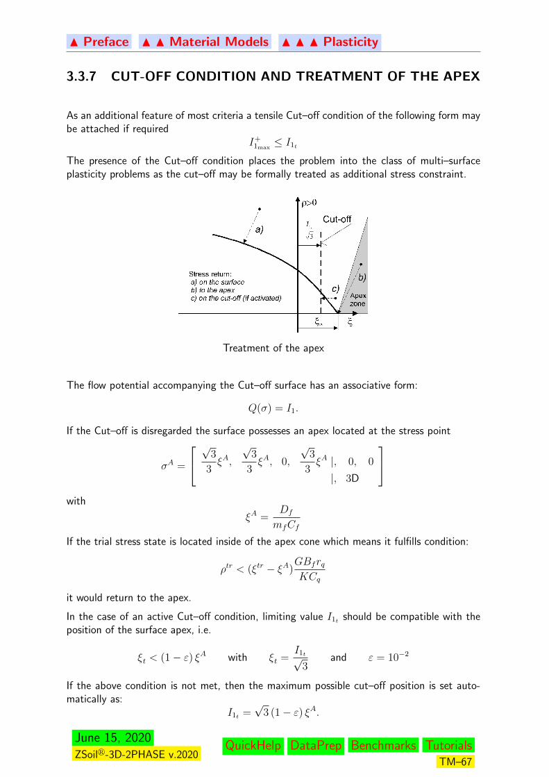
N Preface N N Material Models N N N Plasticity
3.3.7 CUT-OFF CONDITION AND TREATMENT OF THE APEX
As an additional feature of most criteria a tensile Cut–off condition of the following form maybe attached if required
I+1max≤ I1t
The presence of the Cut–off condition places the problem into the class of multi–surfaceplasticity problems as the cut–off may be formally treated as additional stress constraint.
Treatment of the apex
The flow potential accompanying the Cut–off surface has an associative form:
Q(σ) = I1.
If the Cut–off is disregarded the surface possesses an apex located at the stress point
σA =
√3
3ξA,
√3
3ξA, 0,
√3
3ξA |, 0, 0
|, 3D
with
ξA =Df
mfCf
If the trial stress state is located inside of the apex cone which means it fulfills condition:
ρtr < (ξtr − ξA)GBfrqKCq
it would return to the apex.
In the case of an active Cut–off condition, limiting value I1t should be compatible with theposition of the surface apex, i.e.
ξt < (1− ε) ξA with ξt =I1t√
3and ε = 10−2
If the above condition is not met, then the maximum possible cut–off position is set auto-matically as:
I1t =√
3 (1− ε) ξA.
June 15, 2020ZSoilr-3D-2PHASE v.2020
QuickHelp DataPrep Benchmarks TutorialsTM–67
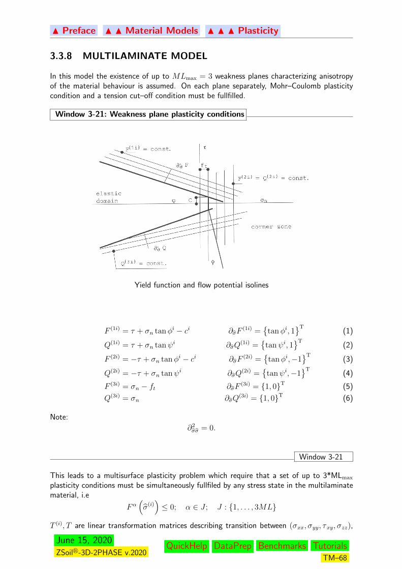
N Preface N N Material Models N N N Plasticity
3.3.8 MULTILAMINATE MODEL
In this model the existence of up to MLmax = 3 weakness planes characterizing anisotropyof the material behaviour is assumed. On each plane separately, Mohr–Coulomb plasticitycondition and a tension cut–off condition must be fullfilled.
Window 3-21: Weakness plane plasticity conditions
Yield function and flow potential isolines
F (1i) = τ + σn tanφi − ci ∂σF(1i) =
tanφi, 1
T(1)
Q(1i) = τ + σn tanψi ∂σQ(1i) =
tanψi, 1
T(2)
F (2i) = −τ + σn tanφi − ci ∂σF(2i) =
tanφi,−1
T(3)
Q(2i) = −τ + σn tanψi ∂σQ(2i) =
tanψi,−1
T(4)
F (3i) = σn − ft ∂σF(3i) = 1, 0T (5)
Q(3i) = σn ∂σQ(3i) = 1, 0T (6)
Note:
∂2σσ = 0.
Window 3-21
This leads to a multisurface plasticity problem which require that a set of up to 3*MLmax
plasticity conditions must be simultaneously fullfiled by any stress state in the multilaminatematerial, i.e
Fα(σ(i))≤ 0; α ∈ J ; J : 1, . . . , 3ML
T (i), T are linear transformation matrices describing transition between (σxx, σyy, τxy, σzz),
June 15, 2020ZSoilr-3D-2PHASE v.2020
QuickHelp DataPrep Benchmarks TutorialsTM–68
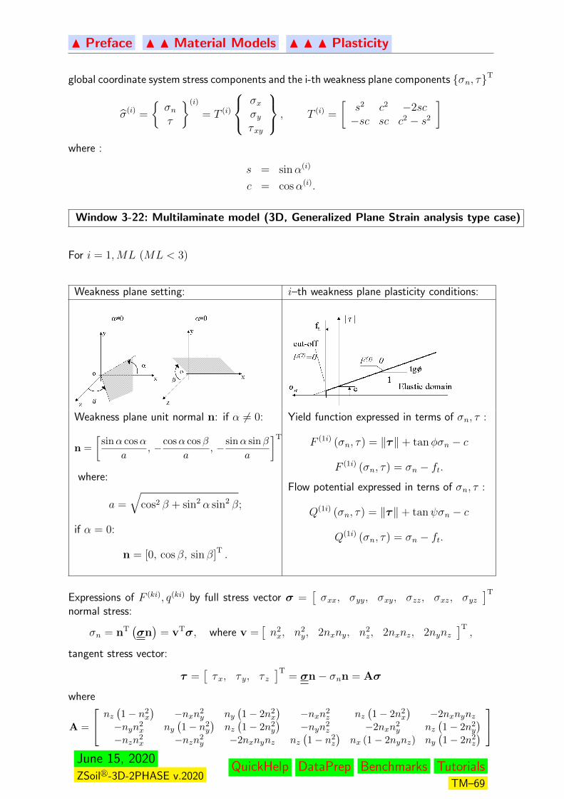
N Preface N N Material Models N N N Plasticity
global coordinate system stress components and the i-th weakness plane components σn, τT
σ(i) =
σnτ
(i)
= T (i)
σxσyτxy
, T (i) =
[s2 c2 −2sc−sc sc c2 − s2
]where :
s = sinα(i)
c = cosα(i).
Window 3-22: Multilaminate model (3D, Generalized Plane Strain analysis type case)
For i = 1,ML (ML < 3)
Weakness plane setting: i–th weakness plane plasticity conditions:
Weakness plane unit normal n: if α 6= 0:
n =
[sinα cosα
a, −cosα cosβ
a, −sinα sinβ
a
]T
where:
a =
√cos2 β + sin2 α sin2 β;
if α = 0:
n = [0, cos β, sin β]T .
Yield function expressed in terms of σn, τ :
F (1i) (σn, τ) = ‖τ‖+ tanφσn − c
F (1i) (σn, τ) = σn − ft.
Flow potential expressed in terns of σn, τ :
Q(1i) (σn, τ) = ‖τ‖+ tanψσn − c
Q(1i) (σn, τ) = σn − ft.
Expressions of F (ki), q(ki) by full stress vector σ =[σxx, σyy, σxy, σzz, σxz, σyz
]Tnormal stress:
σn = nT(σn)
= vTσ, where v =[n2x, n2
y, 2nxny, n2z, 2nxnz, 2nynz
]T,
tangent stress vector:
τ =[τx, τ y, τ z
]T= σn− σnn = Aσ
where
A =
nz(1− n2
x
)−nxn2
y ny(1− 2n2
x
)−nxn2
z nz(1− 2n2
x
)−2nxnynz
−nyn2x ny
(1− n2
y
)nz(1− 2n2
y
)−nyn2
z −2nxn2y nz
(1− 2n2
y
)−nzn2
x −nzn2y −2nxnynz nz
(1− n2
z
)nx (1− 2nynz) ny
(1− 2n2
z
)
June 15, 2020ZSoilr-3D-2PHASE v.2020
QuickHelp DataPrep Benchmarks TutorialsTM–69
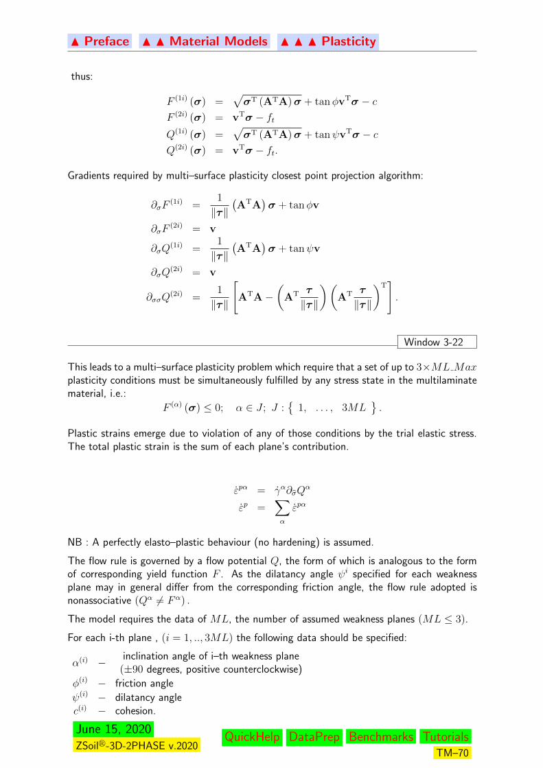
N Preface N N Material Models N N N Plasticity
thus:
F (1i) (σ) =√σT (ATA)σ + tanφvTσ − c
F (2i) (σ) = vTσ − ftQ(1i) (σ) =
√σT (ATA)σ + tanψvTσ − c
Q(2i) (σ) = vTσ − ft.
Gradients required by multi–surface plasticity closest point projection algorithm:
∂σF(1i) =
1
‖τ‖(ATA
)σ + tanφv
∂σF(2i) = v
∂σQ(1i) =
1
‖τ‖(ATA
)σ + tanψv
∂σQ(2i) = v
∂σσQ(2i) =
1
‖τ‖
[ATA−
(AT τ
‖τ‖
)(AT τ
‖τ‖
)T].
Window 3-22
This leads to a multi–surface plasticity problem which require that a set of up to 3×ML Maxplasticity conditions must be simultaneously fulfilled by any stress state in the multilaminatematerial, i.e.:
F (α) (σ) ≤ 0; α ∈ J ; J :
1, . . . , 3ML.
Plastic strains emerge due to violation of any of those conditions by the trial elastic stress.The total plastic strain is the sum of each plane’s contribution.
εpα = γα∂σQα
εp =∑α
εpα
NB : A perfectly elasto–plastic behaviour (no hardening) is assumed.
The flow rule is governed by a flow potential Q, the form of which is analogous to the formof corresponding yield function F . As the dilatancy angle ψi specified for each weaknessplane may in general differ from the corresponding friction angle, the flow rule adopted isnonassociative (Qα 6= Fα) .
The model requires the data of ML, the number of assumed weakness planes (ML ≤ 3).
For each i-th plane , (i = 1, .., 3ML) the following data should be specified:
α(i) − inclination angle of i–th weakness plane(±90 degrees, positive counterclockwise)
φ(i) − friction angle
ψ(i) − dilatancy anglec(i) − cohesion.
June 15, 2020ZSoilr-3D-2PHASE v.2020
QuickHelp DataPrep Benchmarks TutorialsTM–70
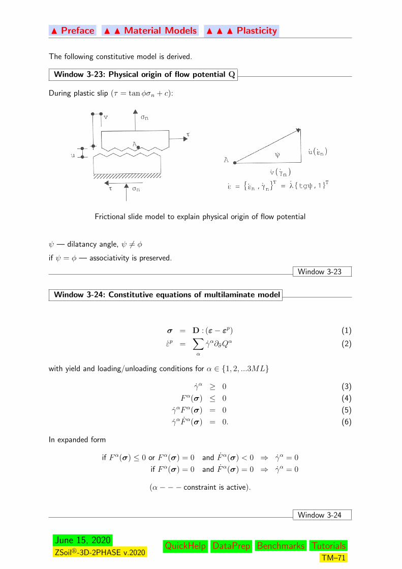
N Preface N N Material Models N N N Plasticity
The following constitutive model is derived.
Window 3-23: Physical origin of flow potential Q
During plastic slip (τ = tanφσn + c):
Frictional slide model to explain physical origin of flow potential
ψ — dilatancy angle, ψ 6= φ
if ψ = φ — associativity is preserved.
Window 3-23
Window 3-24: Constitutive equations of multilaminate model
σ = D : (ε− εp) (1)
εp =∑α
γα∂σQα (2)
with yield and loading/unloading conditions for α ∈ 1, 2, ...3ML
γα ≥ 0 (3)
Fα(σ) ≤ 0 (4)
γαFα(σ) = 0 (5)
γαFα(σ) = 0. (6)
In expanded form
if Fα(σ) ≤ 0 or Fα(σ) = 0 and Fα(σ) < 0 ⇒ γα = 0
if Fα(σ) = 0 and Fα(σ) = 0 ⇒ γα = 0
(α−−− constraint is active).
Window 3-24
June 15, 2020ZSoilr-3D-2PHASE v.2020
QuickHelp DataPrep Benchmarks TutorialsTM–71
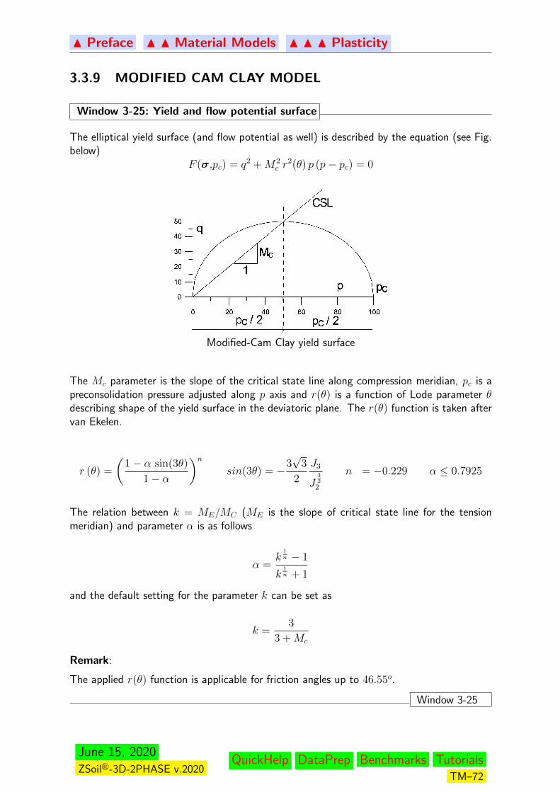
N Preface N N Material Models N N N Plasticity
3.3.9 MODIFIED CAM CLAY MODEL
Window 3-25: Yield and flow potential surface
The elliptical yield surface (and flow potential as well) is described by the equation (see Fig.below)
F (σ,pc) = q2 +M2c r
2(θ) p (p− pc) = 0
Modified-Cam Clay yield surface
The Mc parameter is the slope of the critical state line along compression meridian, pc is apreconsolidation pressure adjusted along p axis and r(θ) is a function of Lode parameter θdescribing shape of the yield surface in the deviatoric plane. The r(θ) function is taken aftervan Ekelen.
r (θ) =
(1− α sin(3θ)
1− α
)nsin(3θ) = −3
√3
2
J3
J322
n = −0.229 α ≤ 0.7925
The relation between k = ME/MC (ME is the slope of critical state line for the tensionmeridian) and parameter α is as follows
α =k
1n − 1
k1n + 1
and the default setting for the parameter k can be set as
k =3
3 +Mc
Remark:
The applied r(θ) function is applicable for friction angles up to 46.55o.
Window 3-25
June 15, 2020ZSoilr-3D-2PHASE v.2020
QuickHelp DataPrep Benchmarks TutorialsTM–72
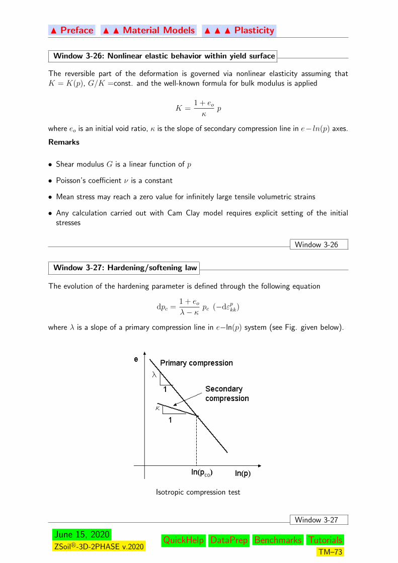
N Preface N N Material Models N N N Plasticity
Window 3-26: Nonlinear elastic behavior within yield surface
The reversible part of the deformation is governed via nonlinear elasticity assuming thatK = K(p), G/K =const. and the well-known formula for bulk modulus is applied
K =1 + eoκ
p
where eo is an initial void ratio, κ is the slope of secondary compression line in e− ln(p) axes.
Remarks
• Shear modulus G is a linear function of p
• Poisson’s coefficient ν is a constant
• Mean stress may reach a zero value for infinitely large tensile volumetric strains
• Any calculation carried out with Cam Clay model requires explicit setting of the initialstresses
Window 3-26
Window 3-27: Hardening/softening law
The evolution of the hardening parameter is defined through the following equation
dpc =1 + eoλ− κ
pc (−dεpkk)
where λ is a slope of a primary compression line in e−ln(p) system (see Fig. given below).
Isotropic compression test
Window 3-27
June 15, 2020ZSoilr-3D-2PHASE v.2020
QuickHelp DataPrep Benchmarks TutorialsTM–73
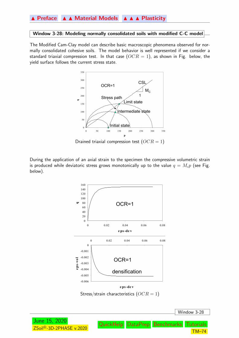
N Preface N N Material Models N N N Plasticity
Window 3-28: Modeling normally consolidated soils with modified C-C model
The Modified Cam-Clay model can describe basic macroscopic phenomena observed for nor-mally consolidated cohesive soils. The model behavior is well represented if we consider astandard triaxial compression test. In that case (OCR = 1), as shown in Fig. below, theyield surface follows the current stress state.
0
50
100
150
200
250
300
350
0 50 100 150 200 250 300 350
p
q
1MC
Stress path
Initial state
Intermediate state
Limit state
CSLOCR=1
Drained triaxial compression test (OCR = 1)
During the application of an axial strain to the specimen the compressive volumetric strainis produced while deviatoric stress grows monotonically up to the value q = Mcp (see Fig.below).
020406080100120140160
0 0.02 0.04 0.06 0.08
e ps -de v
q
-0.006
-0.005
-0.004
-0.003
-0.002
-0.001
00 0.02 0.04 0.06 0.08
e ps -de v
eps-vol
OCR=1
OCR=1
densification
Stress/strain characteristics (OCR = 1)
Window 3-28
June 15, 2020ZSoilr-3D-2PHASE v.2020
QuickHelp DataPrep Benchmarks TutorialsTM–74
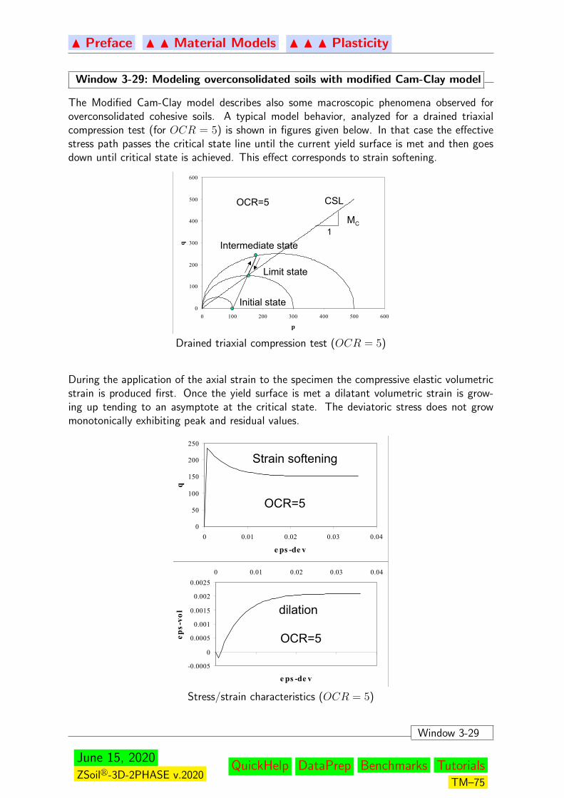
N Preface N N Material Models N N N Plasticity
Window 3-29: Modeling overconsolidated soils with modified Cam-Clay model
The Modified Cam-Clay model describes also some macroscopic phenomena observed foroverconsolidated cohesive soils. A typical model behavior, analyzed for a drained triaxialcompression test (for OCR = 5) is shown in figures given below. In that case the effectivestress path passes the critical state line until the current yield surface is met and then goesdown until critical state is achieved. This effect corresponds to strain softening.
0
100
200
300
400
500
600
0 100 200 300 400 500 600
p
q
MC1
CSL
Initial state
Intermediate state
Limit state
OCR=5
Drained triaxial compression test (OCR = 5)
During the application of the axial strain to the specimen the compressive elastic volumetricstrain is produced first. Once the yield surface is met a dilatant volumetric strain is grow-ing up tending to an asymptote at the critical state. The deviatoric stress does not growmonotonically exhibiting peak and residual values.
0
50
100
150
200
250
0 0.01 0.02 0.03 0.04
e ps -de v
q
-0.0005
0
0.0005
0.001
0.0015
0.002
0.00250 0.01 0.02 0.03 0.04
e ps -de v
eps-vol
OCR=5
OCR=5
Strain softening
dilation
Stress/strain characteristics (OCR = 5)
Window 3-29
June 15, 2020ZSoilr-3D-2PHASE v.2020
QuickHelp DataPrep Benchmarks TutorialsTM–75

N Preface N N Material Models N N N Plasticity
3.3.10 HS-small MODEL
The detailed description of the model is given in the dedicated report.
June 15, 2020ZSoilr-3D-2PHASE v.2020
QuickHelp DataPrep Benchmarks TutorialsTM–76

N Preface N N Material Models N N N Plasticity
3.3.11 Hoek-Brown (true) MODEL
The detailed description of the model is given in the dedicated report.
June 15, 2020ZSoilr-3D-2PHASE v.2020
QuickHelp DataPrep Benchmarks TutorialsTM–77

N Preface N N Material Models N N N Plasticity
3.3.12 Plastic damage MODEL for concrete
A detailed description of the model is given in the dedicated report.
June 15, 2020ZSoilr-3D-2PHASE v.2020
QuickHelp DataPrep Benchmarks TutorialsTM–78
N Preface N N Material Models
3.4 CREEP
Creep is a time–dependent deformation under maintained stress. It is assumed that the stresscan be split into volumetric and deviatoric components and the corresponding time–dependentstrain components are the volumetric and the deviatoric creep. The following formulation isadopted for one–dimensional creep :
εcr = εeinstf(t) = σC (t)
Creep is considered to be proportional to the instantaneous elastic deformation. C(t) is thecreep law corresponding to a unit stress.
The three-dimensional creep law is then:
εcr = ED−1σC(t) = D−1o σC(t)
and C(t) is assumed to be e.g. of the form
C(t) = A(t− t0)m
where A and m are material parameters.
In most situations the same creep law will be adopted for both the volumetric and thedeviatoric components. Different parameters can however be chosen for the volumetric anddeviatoric creep components. Great care has to be taken in that case because this maygenerate a Poisson coefficient which varies in time.
CREEP UNDER VARIABLE STRESS
CREEP PARAMETER IDENTIFICATION FROM EXPERIMENT
June 15, 2020ZSoilr-3D-2PHASE v.2020
QuickHelp DataPrep Benchmarks TutorialsTM–79

N Preface N N Material Models N N N Creep
3.4.1 CREEP UNDER VARIABLE STRESS
Creep under variable stress requires a principle of superposition. The adopted power law doesnot lend itself easily to such in principle. It is therefore replaced, in the implementation, bya series of Kelvin elements. This is described next in Windows 3-31 and 3-30.
The automatic adjustment of the Kelvin element parameters to the prescribed power law isderived in Window .3-32
Window 3-30: Kelvin element under constant unit stress
Constitutive equationq = Gε+ ηε
Creep strain increment, due toq = H(t− t0)
where: H — Heaviside unit step function
εcr =1
G
1− exp
[−Gη
(t− t0)
]= A
1− exp
[− 1
B(t− t0)
]=
= σC(t− t0) with σ = 1
N.B.:εcr = 0 at t = t0
εcr =q
Gat t =∞
Kelvin mechanical model
Window 3-30
June 15, 2020ZSoilr-3D-2PHASE v.2020
QuickHelp DataPrep Benchmarks TutorialsTM–80
N Preface N N Material Models N N N Creep
Window 3-31: Creep under variable stress
Let the creep strain under variable stress be
εcr(t) = D−10
−t∫
τ0
[σ (t)− σ (τ 0)]∂C(t− τ)
∂τdτ
with D0 = E−1D.
For unit stress and a single Kelvin element
C(t, τ) = A
1− exp
[− 1
B(t− τ)
]∂C
∂τ= −A
Bexp
(−t− τ
B
)For a chain of N Kelvin elements in series, and introducing the volumetric-deviatoric split
Cv(t, τ) =N∑i=1
Avi
1− exp
[− 1
Bvi
(t− τ)
]
Cd(t, τ) =N∑i=1
Adi
1− exp
[− 1
Bdi
(t− τ)
]
εcrm(t) =(Dv
0v
)−1
−t∫
τ0
[σm (t)− σm (τ 0)]∂Cv∂τ
dτ
ecr(t) =
(Dd
0
)−1
−t∫
τ0
[s (t)− s (τ 0)]∂Cd∂τ
dτ
The creep strain increment, required by the general nonlinear incremental scheme, as de-scribed in section FULL/MODIFIED NEWTON-RAPHSON ALGORITHM (Section 4.6.1)can be derived by recurrence
∆εcr = εcrn+1 − εcrn = D−10
N∑i=1
∆εcri
and
(∆εi)crn+1 = [σn + θ∆σn+1 − σ (τ 0)]Ai
[1− exp
(−∆tn+1
Bi
)]+
[exp
(−∆tn+1
Bi
)− 1
](εi)
crn
(εi)crn+1 = (εi)
crn + ∆εcri
In the case of nonlinear creep the above recurrence formula is modifed by an additional termscaling the amplitude of the creep strain Ai in the following manner
(∆εi)crn+1 = [σn + θ∆σn+1 − σ (τ 0)] (C1n + θ∆C1n+1)×
Ai
[1− exp
(−∆tn+1
Bi
)]+
[exp
(−∆tn+1
Bi
)− 1
](εi)
crn
June 15, 2020ZSoilr-3D-2PHASE v.2020
QuickHelp DataPrep Benchmarks TutorialsTM–81
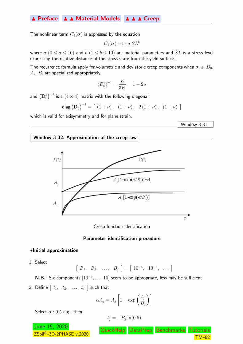
N Preface N N Material Models N N N Creep
The nonlinear term C1(σ) is expressed by the equation
C1(σ) =1+a SLb
where a (0 ≤ a ≤ 10) and b (1 ≤ b ≤ 10) are material parameters and SL is a stress levelexpressing the relative distance of the stress state from the yield surface.
The recurrence formula apply for volumetric and deviatoric creep components when σ, ε, D0,Ai, Bi are specialized appropriately.
(Dv0)−1 =
E
3K= 1− 2ν
and(Dd
0
)−1is a (4× 4) matrix with the following diagonal
diag(Dd
0
)−1=[
(1 + ν) , (1 + ν) , 2 (1 + ν) , (1 + ν)]
which is valid for axisymmetry and for plane strain.
Window 3-31
Window 3-32: Approximation of the creep law
Creep function identification
Parameter identification procedure
•Initial approximation
1. Select [B1, B2, . . . , Bj
]=[
10−4, 10−3, . . .]
N.B.: Six components [10−4, . . . , 10] seem to be appropriate, less may be sufficient
2. Define[t1, t2, . . . tj
]such that
αAj = Aj
[1− exp
(tjBj
)]Select α : 0.5 e.g., then
tj = −Bj ln(0.5)
June 15, 2020ZSoilr-3D-2PHASE v.2020
QuickHelp DataPrep Benchmarks TutorialsTM–82
N Preface N N Material Models N N N Creep
3. Define such that for j = 1 to J
C(tj) =
j−1∑k=1
Ak + Aj
[1− exp
(− tjBj
)]hence
Aj =
[1− exp
(− tjBj
)]−1[C (tj)−
j−1∑k=1
Ak
]
•2nd approximation
A(2) =
[1− exp
(− tjBj
)]−1[C (tj)−
j−1∑k=1
Fk(tj)
]
Fk(tj) = A(1)k
[1− exp
(− tjBj
)].
•Iterative scheme
A(0)j =
[1− exp
(− tjBj
)]−1[C (tj)−
j−1∑k=1
A(0)k
]
•i-th approximation
A(i)j =
[1− exp
(− tjBj
)]−1[C (tj)−
∑k 6=j
Fk(tj)
]
Fk(tj) = A(i−1)k
[1− exp
(− tjBk
)].
tj = −Bj ln (0.5)
Bj = 10j−4 [days] 1 < j < 6.
Convergence test
max
[A
(i)j −
A(i−1)j
A(i)j
]< 10−2
Window 3-32
June 15, 2020ZSoilr-3D-2PHASE v.2020
QuickHelp DataPrep Benchmarks TutorialsTM–83

N Preface N N Material Models N N N Creep
3.4.2 CREEP PARAMETER IDENTIFICATION FROM EXPERI-MENTS
The easiest way to adjust creep parameters A and m for C(t, t0) = A(t − t0)m from anexperimental curve f(t, t0) is to pick two points situated at (t− t0) = 1 for the adjustmentof A and then at a large value of (t− t0) for the adjustment of m.
Depending on the available test the procedure differs only slightly. Four typical experimentsare analyzed next; additional situations can easily be extrapoled using D−1
0 with
D−10 =
1 −ν 0 −ν−ν 1 0 −ν0 0 2(1 + ν) 0−ν −ν 0 1
.If volumetric and deviatoric creep are different i.e.
Cv(t, t0) = Av(t− t0)mv 6= Cd(t, t0) = Ad(t− t0)md
then
(Dv0)−1 =
E
3K= 1− 2ν
and
(Dd
0
)−1=
1 + ν 0 0 0
0 1 + ν 0 00 0 2 (1 + ν) 00 0 0 1 + ν
.
Window 3-33: Uniaxial test
εc = D−10 σC (t− t0)
εc1εc20εc3
=
1 −ν 0 −ν−ν 1 0 −ν0 0 2(1 + ν) 0−ν −ν 0 1
σ1
000
C(t− t0)
hence with
C(t− t0) = A(t− t0)m
εc1 = σ1A(t− t0)m.
Window 3-33
June 15, 2020ZSoilr-3D-2PHASE v.2020
QuickHelp DataPrep Benchmarks TutorialsTM–84

N Preface N N Material Models N N N Creep
Window 3-34: Triaxial test
Assuming εcv is measured in the experiment:εc1εc2γc12
εc3
=
1 −ν 0 −ν−ν 1 0 −ν0 0 2(1 + ν) 0−ν −ν 0 1
σ1
σ2
0σ3
C(t− t0)
hence, with
C(t− t0) = A(t− t0)m
εcv = 3 (1− 2ν)σmA(t− t0)m.
Window 3-34
Window 3-35: Triaxial deviatoric test
Assuming εc2 − εc2 = γc is measured for a unit q = (σ1 − σ2)
εcd = D−10
σ1
σ2
0σ3
and σ3 = σ1
thenεc2 = (σ2 − 2νσ1)C (t, t0)
εc1 = [σ1 − ν (σ2 + σ1)]C (t, t0)
γc = (1 + ν) qC (t− t0) .
Window 3-35
Window 3-36: Oedometer test
εc = D−10
K0σ2
σ2
0K0σ2
C (t, t0)
thenεc2 = (1− 2νK0)σ2C (t, t0) .
Window 3-36
June 15, 2020ZSoilr-3D-2PHASE v.2020
QuickHelp DataPrep Benchmarks TutorialsTM–85

N Preface N N Material Models
3.5 SWELLING
A nonlinear creep approach has been adopted here to model swelling phenomena. Creep seemsto be the simplest phenomenological approach which can reproduce macroscopic behaviour ofswelling soils/rocks both quantitatively and qualitatively without considering all the microscaleeffects.
Oedometric swelling test
Memorizing of in situ stress σ0
Correction of σos with respect to σo state
Three-dimensional generalization
June 15, 2020ZSoilr-3D-2PHASE v.2020
QuickHelp DataPrep Benchmarks TutorialsTM–86
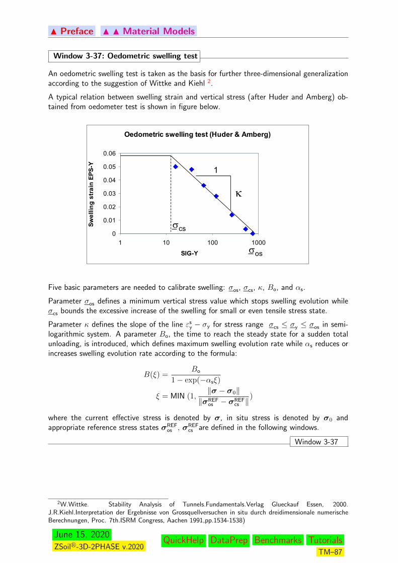
N Preface N N Material Models
Window 3-37: Oedometric swelling test
An oedometric swelling test is taken as the basis for further three-dimensional generalizationaccording to the suggestion of Wittke and Kiehl 2.
A typical relation between swelling strain and vertical stress (after Huder and Amberg) ob-tained from oedometer test is shown in figure below.
Five basic parameters are needed to calibrate swelling: σos, σcs, κ, Bo, and αs.
Parameter σos defines a minimum vertical stress value which stops swelling evolution whileσcs bounds the excessive increase of the swelling for small or even tensile stress state.
Parameter κ defines the slope of the line εsy − σy for stress range σcs ≤ σy ≤ σos in semi-
logarithmic system. A parameter Bo, the time to reach the steady state for a sudden totalunloading, is introduced, which defines maximum swelling evolution rate while αs reduces orincreases swelling evolution rate according to the formula:
B(ξ) =Bo
1− exp(−αsξ)
ξ = MIN (1,‖σ − σ0‖
‖σREFos − σREF
cs ‖)
where the current effective stress is denoted by σ, in situ stress is denoted by σ0 andappropriate reference stress states σREF
os , σREFcs are defined in the following windows.
Window 3-37
2W.Wittke. Stability Analysis of Tunnels.Fundamentals.Verlag Glueckauf Essen, 2000.J.R.Kiehl.Interpretation der Ergebnisse von Grossquellversuchen in situ durch dreidimensionale numerischeBerechnungen, Proc. 7th.ISRM Congress, Aachen 1991,pp.1534-1538)
June 15, 2020ZSoilr-3D-2PHASE v.2020
QuickHelp DataPrep Benchmarks TutorialsTM–87
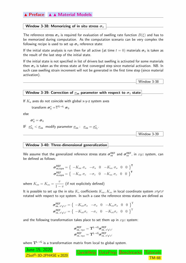
N Preface N N Material Models
Window 3-38: Memorizing of in situ stress σ0
The reference stress σ0 is required for evaluation of swelling rate function B(ξ) and has tobe memorized during computation. As the computation scenario can be very complex thefollowing recipe is used to set up σ0 reference state:
If the initial state analysis is run then for all active (at time t = 0) materials σ0 is taken asthe result of the last step of the initial state.
If the initial state is not specified in list of drivers but swelling is activated for some materialsthen σ0 is taken as the stress state at first converged step since material activation. NB. Insuch case swelling strain increment will not be generated in the first time step (since materialactivation).
Window 3-38
Window 3-39: Correction of σos parameter with respect to σ0 state
If Ko axes do not coincide with global x-y-z system axes
transform σ∗0 =TG→L σ0
else
σ∗0 = σ0
IF σ∗0y< σos modify parameter σos : σos = σ∗0y
.
Window 3-39
Window 3-40: Three-dimensional generalization
We assume that the generalized reference stress state σREFos and σREF
cs , in xyz system, canbe defined as follows:
σREFos,xyz =
−Kox σo −σo 0 −Koz σo 0 0
T
σREFcs,xyz =
−Kox σc −σc 0 −Koz σc 0 0
T
where Kox = Koz =v
1− v(if not explicitely defined)
It is possible to set up the in situ Ko coefficients Kox, Koz in local coordinate system x′y′z′rotated with respect to xyz system. In such a case the reference stress states are defined as
σREFos, x′y′z′ =
−Koxσo −σo 0 −Kozσo 0 0
T
σREFcs, x′y′z′ =
−Koxσc −σc 0 −Kozσc 0 0
T
and the following transformation takes place to set them up in xyz system:
σREFos, xyz = TL→GσREF
os, x′y′z′
σREFcs, xyz = TL→GσREF
cs, x′y′z′
where TL→G is a transformation matrix from local to global system.
June 15, 2020ZSoilr-3D-2PHASE v.2020
QuickHelp DataPrep Benchmarks TutorialsTM–88
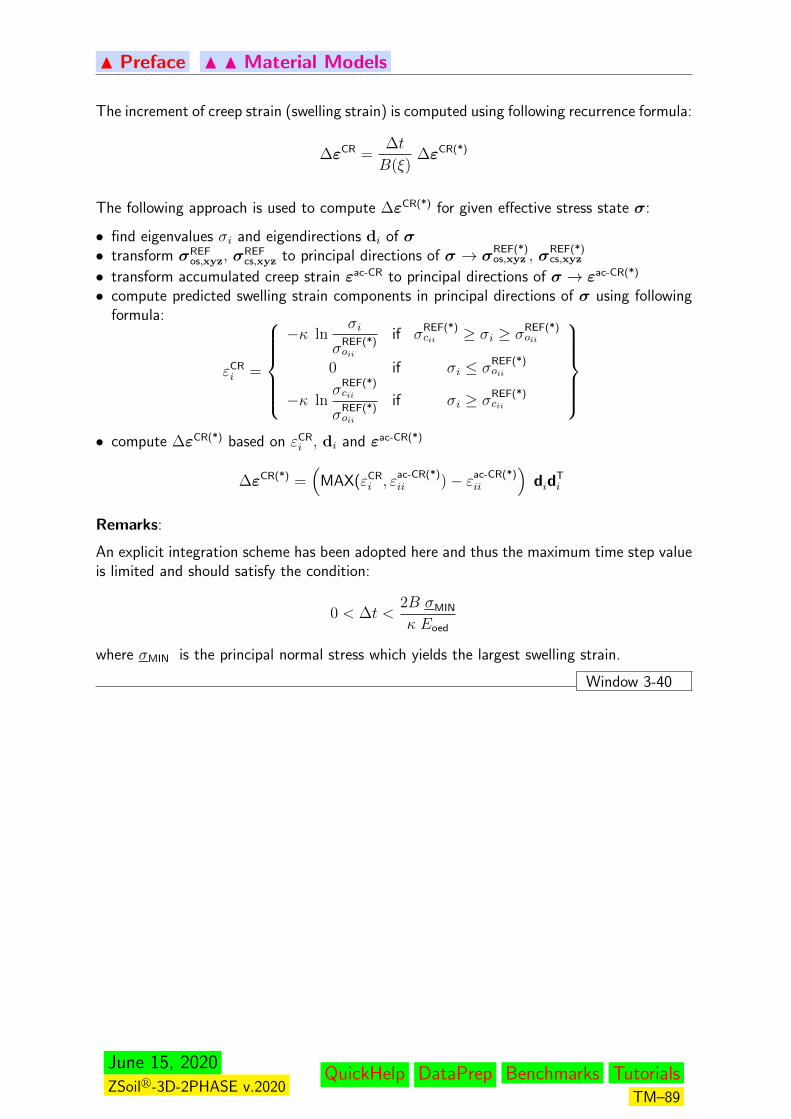
N Preface N N Material Models
The increment of creep strain (swelling strain) is computed using following recurrence formula:
∆εCR =∆t
B(ξ)∆εCR(*)
The following approach is used to compute ∆εCR(*) for given effective stress state σ:
• find eigenvalues σi and eigendirections di of σ• transform σREF
os,xyz, σREFcs,xyz to principal directions of σ → σ
REF(*)os,xyz , σ
REF(*)cs,xyz
• transform accumulated creep strain εac-CR to principal directions of σ → εac-CR(*)
• compute predicted swelling strain components in principal directions of σ using followingformula:
εCRi =
−κ ln
σi
σREF(*)oii
if σREF(*)cii ≥ σi ≥ σ
REF(*)oii
0 if σi ≤ σREF(*)oii
−κ lnσ
REF(*)cii
σREF(*)oii
if σi ≥ σREF(*)cii
• compute ∆εCR(*) based on εCR
i , di and εac-CR(*)
∆εCR(*) =(
MAX(εCRi , ε
ac-CR(*)ii )− εac-CR(*)
ii
)did
Ti
Remarks:
An explicit integration scheme has been adopted here and thus the maximum time step valueis limited and should satisfy the condition:
0 < ∆t <2B σMIN
κ Eoed
where σMIN is the principal normal stress which yields the largest swelling strain.
Window 3-40
June 15, 2020ZSoilr-3D-2PHASE v.2020
QuickHelp DataPrep Benchmarks TutorialsTM–89

N Preface N N Material Models
3.6 AGING CONCRETE
3 The aging concrete model represent time dependent mechanical properties as well as rhe-ological behavior of concrete in early age.
It consists of a set of parallel Maxwell units, as shown in the Window 3-41. Each unit isdescribed by a maturity dependent Young modulus Ek(M) = Wk(M)E, and retardation
time τ k =Ekηk
. The contribution of each unit depends on maturity measure M (expressed
in time units), by the set of weighting factors Wk, (∑
kWk = 1), given for specified timeinstants ti .
Window 3-41: Aging concrete model
Maxwell chain model for aging concrete
Window 3-41
Remarks:
For details of the numerical implementation see:
AGING CONCRETE MODEL - IMPLEMENTATION SCHEME
3concerns versions: ACADEMIC, PROFESSIONAL, EXPERT only
June 15, 2020ZSoilr-3D-2PHASE v.2020
QuickHelp DataPrep Benchmarks TutorialsTM–90

N Preface N N Material Models
3.7 AGING AND CREEP DEDICATED TO PLASTIC DAMAGEMODEL FOR CONCRETE
4
A creep module following the EC2 standard (including aging phenomenon) is fully describedin the report on plastic damage model for concrete. This module can exclusively be usedwith the mentioned constitutive model. Please refer to that document for comprehensiveoverview.
4concerns versions: ACADEMIC, PROFESSIONAL, EXPERT only
June 15, 2020ZSoilr-3D-2PHASE v.2020
QuickHelp DataPrep Benchmarks TutorialsTM–91

N Preface N N Material Models
3.8 APPENDICES
SAFETY FACTORS AND STRESS LEVELS
June 15, 2020ZSoilr-3D-2PHASE v.2020
QuickHelp DataPrep Benchmarks TutorialsTM–92

N Preface N N Material Models N N N Appendix
3.8.1 SAFETY FACTORS AND STRESS LEVELS
The following definitions are used in ZSoilr; of course these definitions are not unique.
Window 3-42: Stress level (SL)
I. for axisymmetric criteria
SL =q
qfailurewith q =
√3J2
II. for Lode’s angle dependent criteria
SL =1
λwith σfailure = σmδ + λs
Remarks:
1. I is a subset of II
2. obviously λ will be different for each material point.
Window 3-42
Window 3-43: Safety factor (SF)
I. Let SF1 be the multiplier which can be applied uniformly to each deviatoric stress in thestructure, such that failure occurs when
σ′ = σmδ + SF1s
II. For two–parameter criteria (C, φ) an alternative definition is available which is
SF2 =
∣∣∣∣∫
Γτ failuredΓ∫Γτ dΓ
∣∣∣∣where Γ is the failure surface and can, as shown elsewhere, be obtained numerically by aprogressive reduction of C and tanφ using:
c′ =c
SF2
(tanφ)′ =tanφ
SF2
.
In the general Mentrey–Willam definition this amounts to replace the parameters of thecriterion by
A′f = SF1 Af
B′f = SF1 Bf
Window 3-43
June 15, 2020ZSoilr-3D-2PHASE v.2020
QuickHelp DataPrep Benchmarks TutorialsTM–93

N Preface N N Material Models N N N Appendix
June 15, 2020ZSoilr-3D-2PHASE v.2020
QuickHelp DataPrep Benchmarks TutorialsTM–94

N Preface
Chapter 4
NUMERICAL IMPLEMENTATION
WEAK FORMULATION
ELEMENTS
INCOMPRESSIBLE AND DILATANT MEDIA
FAR FIELD
OVERLAID MESHES
ALGORITHMS
June 15, 2020ZSoilr-3D-2PHASE v.2020
QuickHelp DataPrep Benchmarks TutorialsTM–95

N Preface N N Numerical Implementation
4.1 WEAK FORM AND MATRIX FORMS OF THE PROBLEM
SINGLE PHASE MEDIUM, TIME INDEPENDENT LOADING
TWO–PHASE MEDIUM, RHEOLOGICAL BEHAVIOUR
HEAT TRANSFER
In the subsequent sections the following Hughes notations is used:
w(i,j) =1
2(wi,j + wj,i)
June 15, 2020ZSoilr-3D-2PHASE v.2020
QuickHelp DataPrep Benchmarks TutorialsTM–96
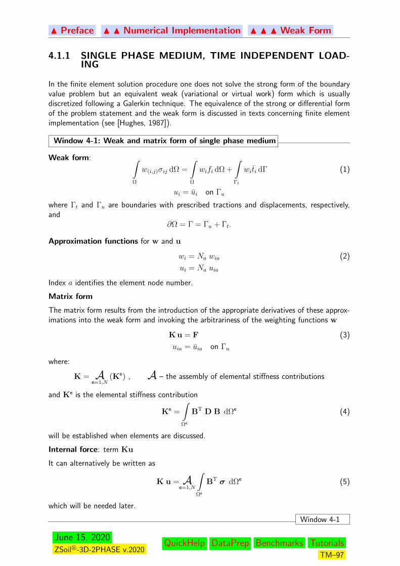
N Preface N N Numerical Implementation N N N Weak Form
4.1.1 SINGLE PHASE MEDIUM, TIME INDEPENDENT LOAD-ING
In the finite element solution procedure one does not solve the strong form of the boundaryvalue problem but an equivalent weak (variational or virtual work) form which is usuallydiscretized following a Galerkin technique. The equivalence of the strong or differential formof the problem statement and the weak form is discussed in texts concerning finite elementimplementation (see [Hughes, 1987]).
Window 4-1: Weak and matrix form of single phase medium
Weak form: ∫Ω
w(i,j)σij dΩ =
∫Ω
wifi dΩ +
∫Γt
witi dΓ (1)
ui = ui on Γu
where Γt and Γu are boundaries with prescribed tractions and displacements, respectively,and
∂Ω = Γ = Γu + Γt.
Approximation functions for w and u
wi = Na wia (2)
ui = Na uia
Index a identifies the element node number.
Matrix form
The matrix form results from the introduction of the appropriate derivatives of these approx-imations into the weak form and invoking the arbitrariness of the weighting functions w
K u = F (3)
uia = uia on Γu
where:
K = Ae=1,N
(Ke) , A – the assembly of elemental stiffness contributions
and Ke is the elemental stiffness contribution
Ke =
∫Ωe
BT D B dΩe (4)
will be established when elements are discussed.
Internal force: term Ku
It can alternatively be written as
K u = Ae=1,N
∫Ωe
BT σ dΩe (5)
which will be needed later.
Window 4-1
June 15, 2020ZSoilr-3D-2PHASE v.2020
QuickHelp DataPrep Benchmarks TutorialsTM–97
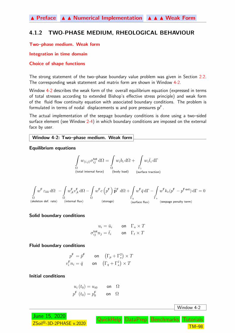
N Preface N N Numerical Implementation N N N Weak Form
4.1.2 TWO-PHASE MEDIUM, RHEOLOGICAL BEHAVIOUR
Two–phase medium. Weak form
Integration in time domain
Choice of shape functions
The strong statement of the two–phase boundary value problem was given in Section 2.2.The corresponding weak statement and matrix form are shown in Window 4-2.
Window 4-2 describes the weak form of the overall equilibrium equation (expressed in termsof total stresses according to extended Bishop’s effective stress principle) and weak formof the fluid flow continuity equation with associated boundary conditions. The problem isformulated in terms of nodal displacements u and pore pressures pF .
The actual implementation of the seepage boundary conditions is done using a two–sidedsurface element (see Window 2-4) in which boundary conditions are imposed on the externalface by user.
Window 4-2: Two–phase medium. Weak form
Equilibrium equations∫Ω
w(i,j)σtotij dΩ
(total internal force)
=
∫Ω
wibi dΩ
(body load)
+
∫Γt
witi dΓ
(surface traction)
∫Ω
wF εkk dΩ
(skeleton def. rate)
−∫Ω
wF,kv
F,k dΩ
(internal flux)
−∫Ω
wFc(pF) pF dΩ
(storage)
+
∫Γq
wFq dΓ
(surface flux)
−∫Γs
wFkv(pF − pF ext) dΓ
(seepage penalty term)
= 0
Solid boundary conditions
ui = ui on Γu × Tσtotij nj = ti on Γt × T
Fluid boundary conditions
pF = pF on(Γp + Γ2
s
)× T
vFi ni = q on
(Γq + Γ1
s
)× T
Initial conditions
ui (t0) = ui0 on Ω
pF (t0) = pF0 on Ω
Window 4-2
June 15, 2020ZSoilr-3D-2PHASE v.2020
QuickHelp DataPrep Benchmarks TutorialsTM–98

N Preface N N Numerical Implementation N N N Weak Form
The matrix form of the problem results from the specific choice of shape functions for inter-polation of displacements and pore pressure fields within the element. The application ofthe implicit integration scheme in time permits an elimination of time derivatives from set oflinearized equations which is finally solved for ∆u the increment of displacement u and ∆pF
the increment of pore pressure pF . Iterations are needed if the constitutive law of the solidskeleton is nonlinear.
Window 4-3: Integration in time domain
The following predictor-corrector scheme has been adopted for integration of the displace-ments and pore pressures in time.
uiN+1= uiN + (1− θ) ∆t uiN + θ ∆t uiN+1
= uiN + ∆t uiN︸ ︷︷ ︸upredictoriN+1
+θ∆t ∆uiN+1︸ ︷︷ ︸uiN+1
− uiNpN+1 = pN + (1− θ) ∆t pN + θ ∆t pN+1 = pN + ∆t pN︸ ︷︷ ︸ppredictorN+1
+θ∆t ∆pN+1︸ ︷︷ ︸
pN+1− p
N
The integration coefficient θ has been assumed to satisfy the sufficient condition for stability
θ ≥ 1
2.
Window 4-3
Window 4-4: Choice of shape functions
Let us introduce the following finite element interpolation functions for approximated field(s),i.e. displacements uh and pore pressure ph, within a finite element
uh = Nuue wh = Nuwe ph = Nppe qh = Npqe
With these definitions the strain-displacement relation is expressed in the standard form
ε(uh)
= B ue
Window 4-4
June 15, 2020ZSoilr-3D-2PHASE v.2020
QuickHelp DataPrep Benchmarks TutorialsTM–99
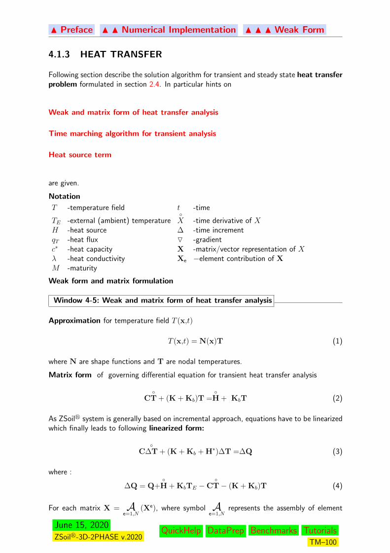
N Preface N N Numerical Implementation N N N Weak Form
4.1.3 HEAT TRANSFER
Following section describe the solution algorithm for transient and steady state heat transferproblem formulated in section 2.4. In particular hints on
Weak and matrix form of heat transfer analysis
Time marching algorithm for transient analysis
Heat source term
are given.
Notation
T -temperature field t -time
TE -external (ambient) temperatureX -time derivative of X
H -heat source ∆ -time incrementqT -heat flux O -gradientc∗ -heat capacity X -matrix/vector representation of Xλ -heat conductivity Xe −element contribution of XM -maturity
Weak form and matrix formulation
Window 4-5: Weak and matrix form of heat transfer analysis
Approximation for temperature field T (x,t)
T (x,t) = N(x)T (1)
where N are shape functions and T are nodal temperatures.
Matrix form of governing differential equation for transient heat transfer analysis
CT + (K + Kb)T =
H + KbT (2)
As ZSoilr system is generally based on incremental approach, equations have to be linearizedwhich finally leads to following linearized form:
C
∆T + (K + Kb + H∗)∆T =∆Q (3)
where :
∆Q = Q+H + KbTE −C
T− (K + Kb)T (4)
For each matrix X = Ae=1,N
(Xe), where symbol Ae=1,N
represents the assembly of element
June 15, 2020ZSoilr-3D-2PHASE v.2020
QuickHelp DataPrep Benchmarks TutorialsTM–100
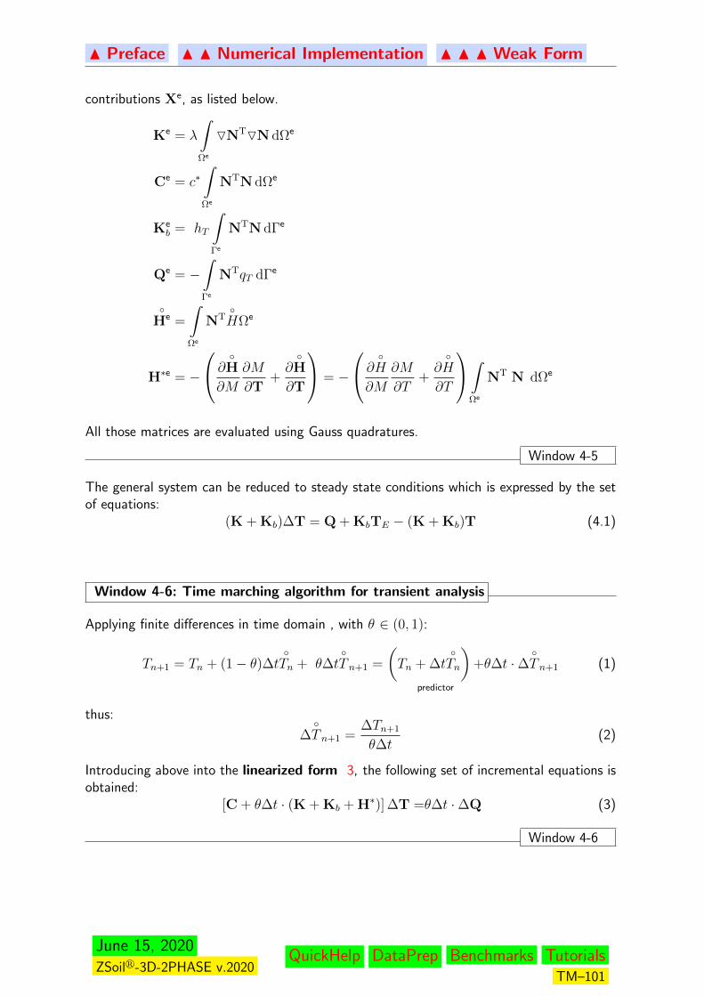
N Preface N N Numerical Implementation N N N Weak Form
contributions Xe, as listed below.
Ke = λ
∫Ωe
ONTON dΩe
Ce = c∗∫Ωe
NTN dΩe
Keb = hT
∫Γe
NTN dΓe
Qe = −∫Γe
NTqT dΓe
He =
∫Ωe
NTHΩe
H∗e = −
∂H
∂M
∂M
∂T+∂H
∂T
= −
∂H
∂M
∂M
∂T+∂H
∂T
∫Ωe
NT N dΩe
All those matrices are evaluated using Gauss quadratures.
Window 4-5
The general system can be reduced to steady state conditions which is expressed by the setof equations:
(K + Kb)∆T = Q + KbTE − (K + Kb)T (4.1)
Window 4-6: Time marching algorithm for transient analysis
Applying finite differences in time domain , with θ ∈ (0, 1):
Tn+1 = Tn + (1− θ)∆tTn + θ∆t
T n+1 =
(Tn + ∆t
Tn
)+
predictor
θ∆t ·∆T n+1 (1)
thus:
∆T n+1 =
∆Tn+1
θ∆t(2)
Introducing above into the linearized form 3, the following set of incremental equations isobtained:
[C + θ∆t · (K + Kb + H∗)] ∆T =θ∆t ·∆Q (3)
Window 4-6
June 15, 2020ZSoilr-3D-2PHASE v.2020
QuickHelp DataPrep Benchmarks TutorialsTM–101
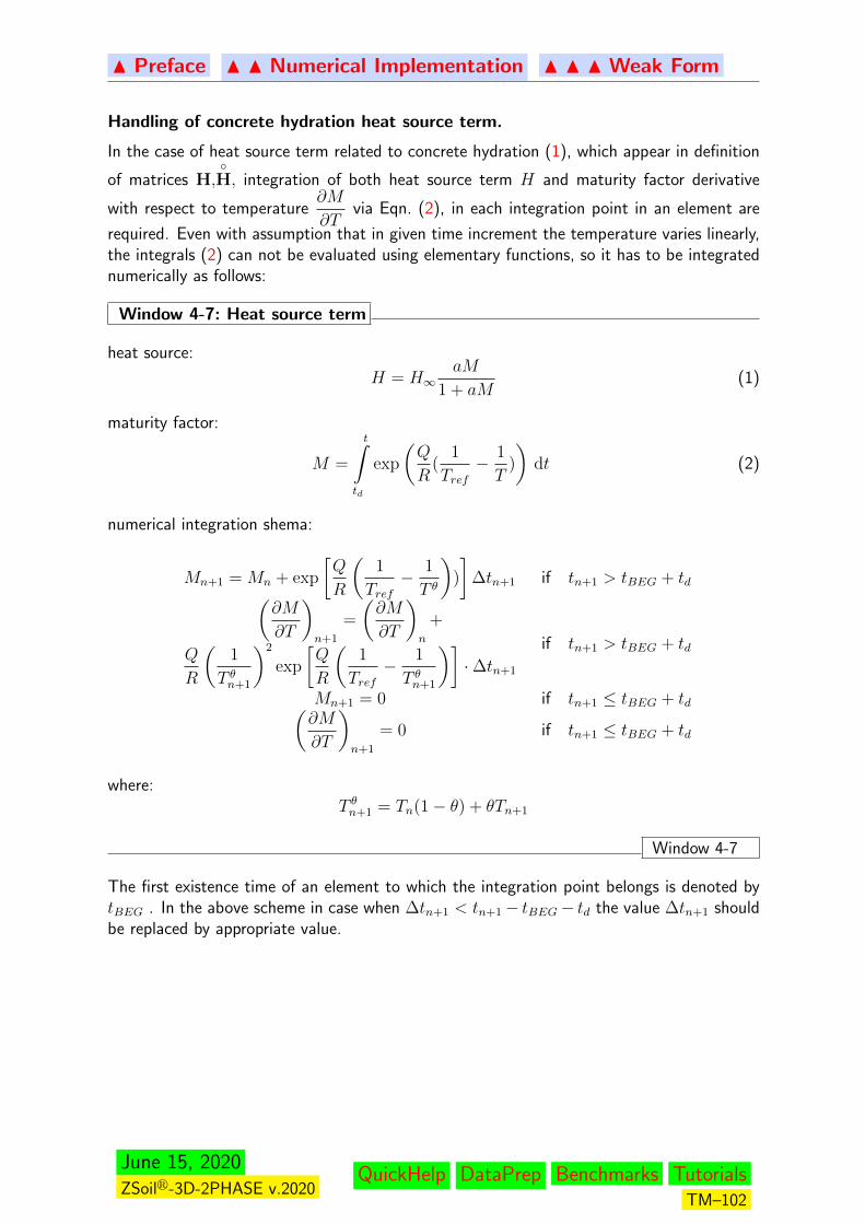
N Preface N N Numerical Implementation N N N Weak Form
Handling of concrete hydration heat source term.
In the case of heat source term related to concrete hydration (1), which appear in definition
of matrices H,H, integration of both heat source term H and maturity factor derivative
with respect to temperature∂M
∂Tvia Eqn. (2), in each integration point in an element are
required. Even with assumption that in given time increment the temperature varies linearly,the integrals (2) can not be evaluated using elementary functions, so it has to be integratednumerically as follows:
Window 4-7: Heat source term
heat source:
H = H∞aM
1 + aM(1)
maturity factor:
M =
t∫td
exp
(Q
R(
1
Tref− 1
T)
)dt (2)
numerical integration shema:
Mn+1 = Mn + exp
[Q
R
(1
Tref− 1
T θ
))
]∆tn+1 if tn+1 > tBEG + td(
∂M
∂T
)n+1
=
(∂M
∂T
)n
+
Q
R
(1
T θn+1
)2
exp
[Q
R
(1
Tref− 1
T θn+1
)]·∆tn+1
if tn+1 > tBEG + td
Mn+1 = 0 if tn+1 ≤ tBEG + td(∂M
∂T
)n+1
= 0 if tn+1 ≤ tBEG + td
where:T θn+1 = Tn(1− θ) + θTn+1
Window 4-7
The first existence time of an element to which the integration point belongs is denoted bytBEG . In the above scheme in case when ∆tn+1 < tn+1− tBEG− td the value ∆tn+1 shouldbe replaced by appropriate value.
June 15, 2020ZSoilr-3D-2PHASE v.2020
QuickHelp DataPrep Benchmarks TutorialsTM–102

N Preface N N Numerical Implementation
4.2 ELEMENTS
FINITE ELEMENTS FOR 2D/3D CONTINUUM PROBLEMS
NUMERICAL INTEGRATION
STRAINS
STIFFNESS
BODY FORCES
INITIAL STRESSES
June 15, 2020ZSoilr-3D-2PHASE v.2020
QuickHelp DataPrep Benchmarks TutorialsTM–103
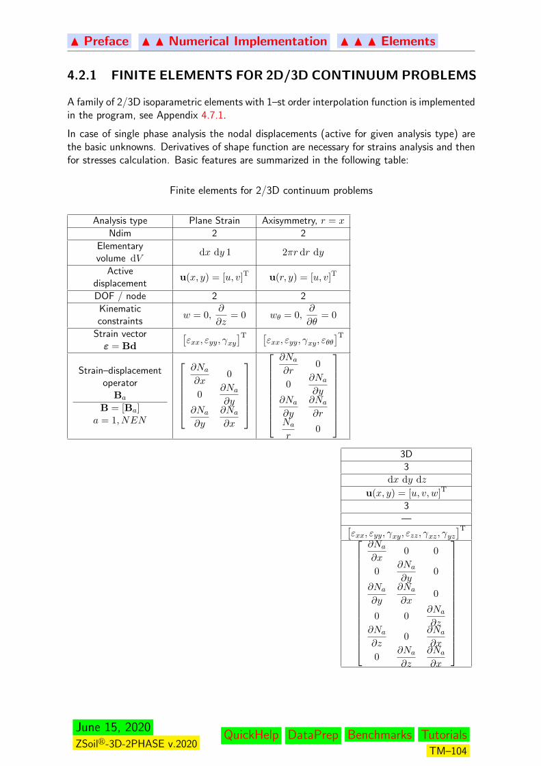
N Preface N N Numerical Implementation N N N Elements
4.2.1 FINITE ELEMENTS FOR 2D/3D CONTINUUM PROBLEMS
A family of 2/3D isoparametric elements with 1–st order interpolation function is implementedin the program, see Appendix 4.7.1.
In case of single phase analysis the nodal displacements (active for given analysis type) arethe basic unknowns. Derivatives of shape function are necessary for strains analysis and thenfor stresses calculation. Basic features are summarized in the following table:
Finite elements for 2/3D continuum problems
Analysis type Plane Strain Axisymmetry, r = x
Ndim 2 2
Elementaryvolume dV
dx dy 1 2πr dr dy
Activedisplacement
u(x, y) = [u, v]T u(r, y) = [u, v]T
DOF / node 2 2
Kinematicconstraints
w = 0,∂
∂z= 0 wθ = 0,
∂
∂θ= 0
Strain vectorε = Bd
[εxx, εyy, γxy
]T [εxx, εyy, γxy, εθθ
]TStrain–displacement
operatorBa
B = [Ba]a = 1, NEN
∂Na
∂x0
0∂Na
∂y∂Na
∂y
∂Na
∂x
∂Na
∂r0
0∂Na
∂y∂Na
∂y
∂Na
∂rNa
r0
3D
3
dx dy dz
u(x, y) = [u, v, w]T
3
—[εxx, εyy, γxy, εzz, γxz, γyz
]T
∂Na
∂x0 0
0∂Na
∂y0
∂Na
∂y
∂Na
∂x0
0 0∂Na
∂z∂Na
∂z0
∂Na
∂x
0∂Na
∂z
∂Na
∂x
June 15, 2020ZSoilr-3D-2PHASE v.2020
QuickHelp DataPrep Benchmarks TutorialsTM–104
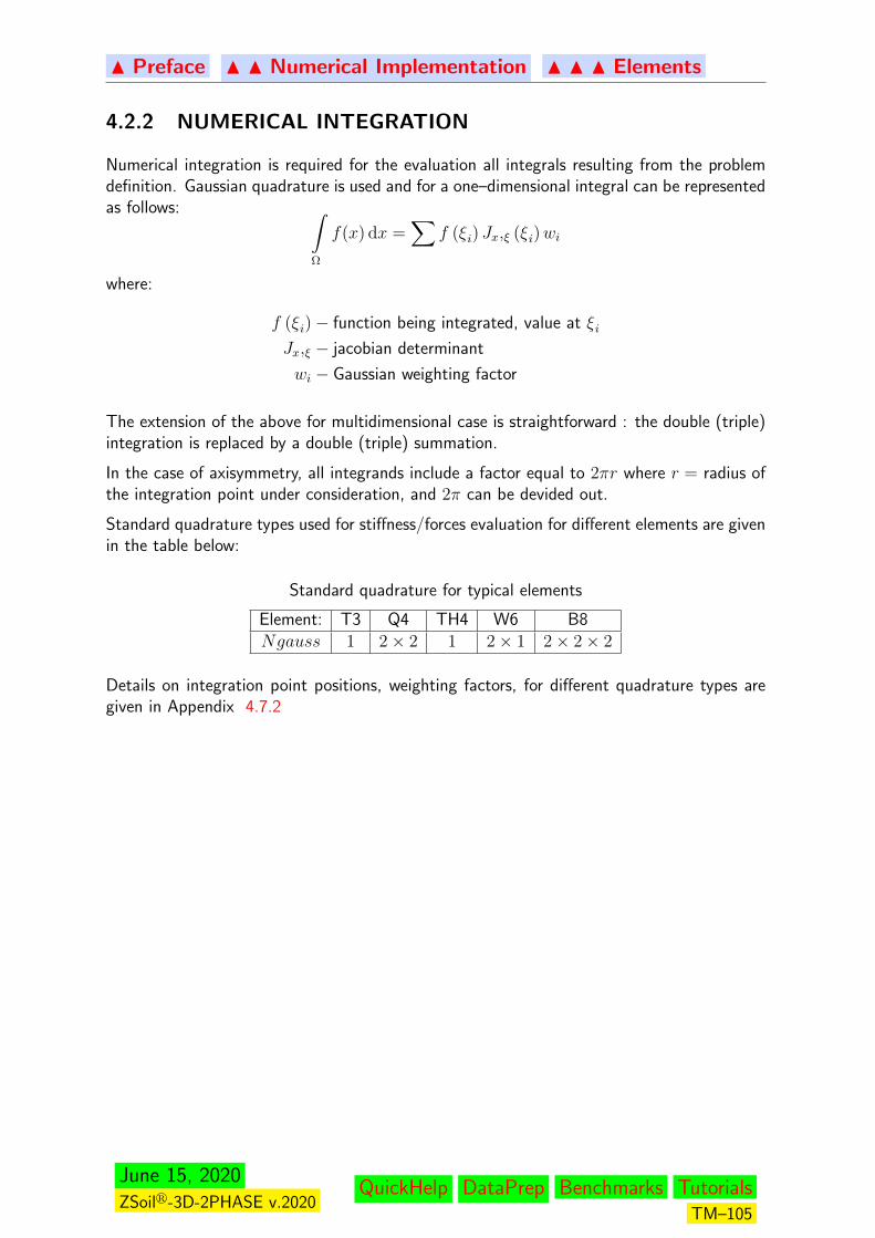
N Preface N N Numerical Implementation N N N Elements
4.2.2 NUMERICAL INTEGRATION
Numerical integration is required for the evaluation all integrals resulting from the problemdefinition. Gaussian quadrature is used and for a one–dimensional integral can be representedas follows: ∫
Ω
f(x) dx =∑
f (ξi) Jx,ξ (ξi)wi
where:
f (ξi)− function being integrated, value at ξiJx,ξ − jacobian determinant
wi − Gaussian weighting factor
The extension of the above for multidimensional case is straightforward : the double (triple)integration is replaced by a double (triple) summation.
In the case of axisymmetry, all integrands include a factor equal to 2πr where r = radius ofthe integration point under consideration, and 2π can be devided out.
Standard quadrature types used for stiffness/forces evaluation for different elements are givenin the table below:
Standard quadrature for typical elements
Element: T3 Q4 TH4 W6 B8Ngauss 1 2× 2 1 2× 1 2× 2× 2
Details on integration point positions, weighting factors, for different quadrature types aregiven in Appendix 4.7.2
June 15, 2020ZSoilr-3D-2PHASE v.2020
QuickHelp DataPrep Benchmarks TutorialsTM–105
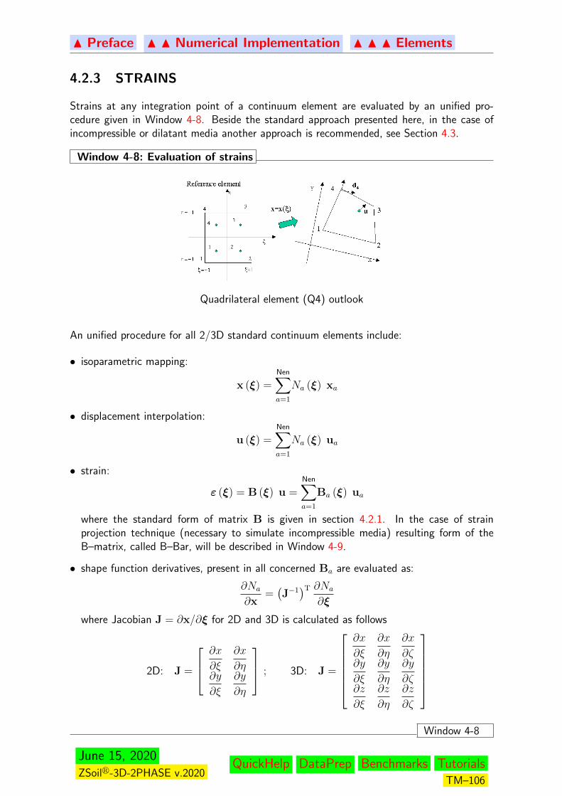
N Preface N N Numerical Implementation N N N Elements
4.2.3 STRAINS
Strains at any integration point of a continuum element are evaluated by an unified pro-cedure given in Window 4-8. Beside the standard approach presented here, in the case ofincompressible or dilatant media another approach is recommended, see Section 4.3.
Window 4-8: Evaluation of strains
Quadrilateral element (Q4) outlook
An unified procedure for all 2/3D standard continuum elements include:
• isoparametric mapping:
x (ξ) =Nen∑a=1
Na (ξ) xa
• displacement interpolation:
u (ξ) =Nen∑a=1
Na (ξ) ua
• strain:
ε (ξ) = B (ξ) u =Nen∑a=1
Ba (ξ) ua
where the standard form of matrix B is given in section 4.2.1. In the case of strainprojection technique (necessary to simulate incompressible media) resulting form of theB–matrix, called B–Bar, will be described in Window 4-9.
• shape function derivatives, present in all concerned Ba are evaluated as:
∂Na
∂x=(J−1)T ∂Na
∂ξ
where Jacobian J = ∂x/∂ξ for 2D and 3D is calculated as follows
2D: J =
∂x
∂ξ
∂x
∂η∂y
∂ξ
∂y
∂η
; 3D: J =
∂x
∂ξ
∂x
∂η
∂x
∂ζ∂y
∂ξ
∂y
∂η
∂y
∂ζ∂z
∂ξ
∂z
∂η
∂z
∂ζ
Window 4-8
June 15, 2020ZSoilr-3D-2PHASE v.2020
QuickHelp DataPrep Benchmarks TutorialsTM–106
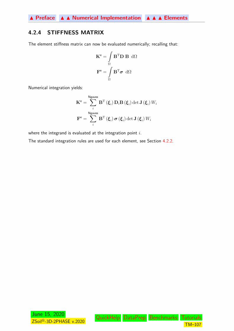
N Preface N N Numerical Implementation N N N Elements
4.2.4 STIFFNESS MATRIX
The element stiffness matrix can now be evaluated numerically; recalling that:
Ke =
∫Ω
BTD B dΩ
Fe =
∫Ω
BTσ dΩ
Numerical integration yields:
Ke =
Ngauss∑i
BT (ξi) DiB (ξi) det J (ξi)Wi
Fe =
Ngauss∑i
BT (ξi)σ (ξi) det J (ξi)Wi
where the integrand is evaluated at the integration point i.
The standard integration rules are used for each element, see Section 4.2.2.
June 15, 2020ZSoilr-3D-2PHASE v.2020
QuickHelp DataPrep Benchmarks TutorialsTM–107

N Preface N N Numerical Implementation N N N Elements
4.2.5 BODY FORCES AND DISTRIBUTED LOADS
The introduction of the interpolation functions into the weak form yields an elemental bodyforce term as follows:
Feb =
∫Ωe
NTb dΩe
For distributed forces, the equivalent nodal force is seen to be:
Fet =
∫∂Γe
NTt dΓe.
June 15, 2020ZSoilr-3D-2PHASE v.2020
QuickHelp DataPrep Benchmarks TutorialsTM–108
N Preface N N Numerical Implementation N N N Elements
4.2.6 INITIAL STRESSES, STRAINS
If the initial stress field is in equilibrium the initial stresses can simply be added to the stressesresulting from deformations. If not, equivalent nodal forces must be calculated. Nodal forcesequivalent to initial stresses and/or strains can be introduced as follows; this calls for ageneralized stress-strain relation.
Letσ = D (ε− ε0) + σ0
where σ0 are the initial stresses and ε0 are the initial strains. By the definition of the internalforce term:
Ae=1,N
∫Ω
BTσ dΩ = Ae=1,N
∫Ω
BTD (ε− ε0) dΩ + Ae=1,N
∫Ω
BTσ0 dΩ
from which the following expression of the nonlinear equilibrium equation results
Fint (u) = F− Fε + Fσ0
with
Fσ0 = Ae=1,N
∫Ω
BTσ0 dΩ
Fε = Ae=1,N
∫Ω
BTε0 dΩ.
Note that if initial stresses are in equilibrium Fσ0 = 0 no deformations will result from theinitial stresses. If not, deformations will result. Similarly if initial strains are compatible withboundary conditions, no stresses result.
June 15, 2020ZSoilr-3D-2PHASE v.2020
QuickHelp DataPrep Benchmarks TutorialsTM–109

N Preface N N Numerical Implementation
4.3 INCOMPRESSIBLE AND DILATANT MEDIA
A strain projection technique is necessary in order to simulate incompressible media. Theresulting form of the B–matrix, called B–Bar, will be described later on.
Another finite element technique to simulate incompressible and highly dilatant plastic mediais the Enhanced Assumed Strain method (EAS). The general idea and detailed algorithmicscheme is described in Section 4.3.2. This option is activated in ZSOIL when dilatant plasticflow is active.
INCOMPRESSIBLE MEDIA: B-BAR STRAIN PROJECTION METHOD
DILATANT MEDIA: ENHANCED ASSUMED STRAIN METHOD
June 15, 2020ZSoilr-3D-2PHASE v.2020
QuickHelp DataPrep Benchmarks TutorialsTM–110
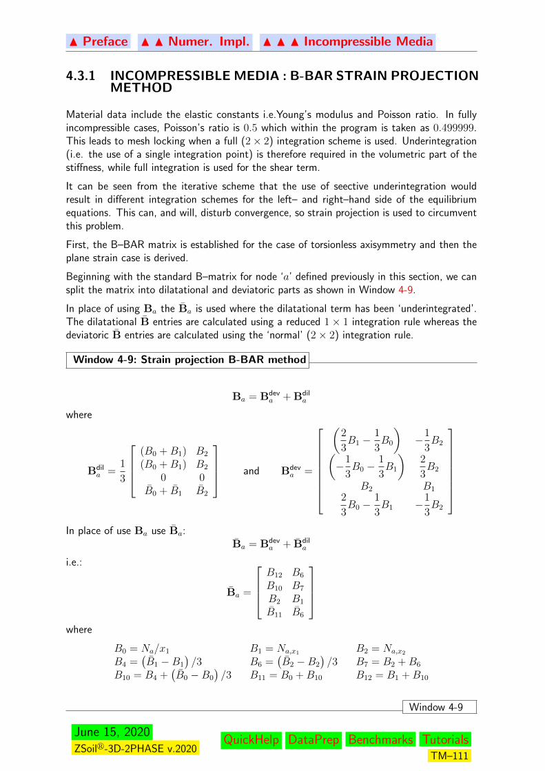
N Preface N N Numer. Impl. N N N Incompressible Media
4.3.1 INCOMPRESSIBLE MEDIA : B-BAR STRAIN PROJECTIONMETHOD
Material data include the elastic constants i.e.Young’s modulus and Poisson ratio. In fullyincompressible cases, Poisson’s ratio is 0.5 which within the program is taken as 0.499999.This leads to mesh locking when a full (2× 2) integration scheme is used. Underintegration(i.e. the use of a single integration point) is therefore required in the volumetric part of thestiffness, while full integration is used for the shear term.
It can be seen from the iterative scheme that the use of seective underintegration wouldresult in different integration schemes for the left– and right–hand side of the equilibriumequations. This can, and will, disturb convergence, so strain projection is used to circumventthis problem.
First, the B–BAR matrix is established for the case of torsionless axisymmetry and then theplane strain case is derived.
Beginning with the standard B–matrix for node ‘a’ defined previously in this section, we cansplit the matrix into dilatational and deviatoric parts as shown in Window 4-9.
In place of using Ba the Ba is used where the dilatational term has been ‘underintegrated’.The dilatational B entries are calculated using a reduced 1× 1 integration rule whereas thedeviatoric B entries are calculated using the ‘normal’ (2× 2) integration rule.
Window 4-9: Strain projection B-BAR method
Ba = Bdeva + Bdil
a
where
Bdila =
1
3
(B0 +B1) B2
(B0 +B1) B2
0 0B0 + B1 B2
and Bdeva =
(2
3B1 −
1
3B0
)−1
3B2(
−1
3B0 −
1
3B1
)2
3B2
B2 B1
2
3B0 −
1
3B1 −1
3B2
In place of use Ba use Ba:
Ba = Bdeva + Bdil
a
i.e.:
Ba =
B12 B6
B10 B7
B2 B1
B11 B6
where
B0 = Na/x1 B1 = Na,x1 B2 = Na,x2
B4 =(B1 −B1
)/3 B6 =
(B2 −B2
)/3 B7 = B2 +B6
B10 = B4 +(B0 −B0
)/3 B11 = B0 +B10 B12 = B1 +B10
Window 4-9
June 15, 2020ZSoilr-3D-2PHASE v.2020
QuickHelp DataPrep Benchmarks TutorialsTM–111

N Preface N N Numer. Impl. N N N Incompressible Media
Remarks:
1. The plane strain case many be obtained from the above formulation by simply settingB0 = B0 = 0 and using Cartesian rather than cylindrical coordinates. The 2πr (or r)factor included in the integrands in the case of axisymmetry must also be ignored.
2. Notice that the D matrix remains 4× 4 for plane strain, when B the formulation is used.
June 15, 2020ZSoilr-3D-2PHASE v.2020
QuickHelp DataPrep Benchmarks TutorialsTM–112

N Preface N N Numer. Impl. N N N Incompressible Media
4.3.2 DILATANT MEDIA: ENHANCED ASSUMED STRAIN METHOD
INTRODUCTION TO ENHANCED ASSSUMED STRAIN (EAS) APPROACH
EXTENSION OF EAS TO NONLINEAR ELASTO–PLASTIC ANALYSIS
REMARKS AND ASSESSMENT OF EAS ELEMENTS
June 15, 2020ZSoilr-3D-2PHASE v.2020
QuickHelp DataPrep Benchmarks TutorialsTM–113
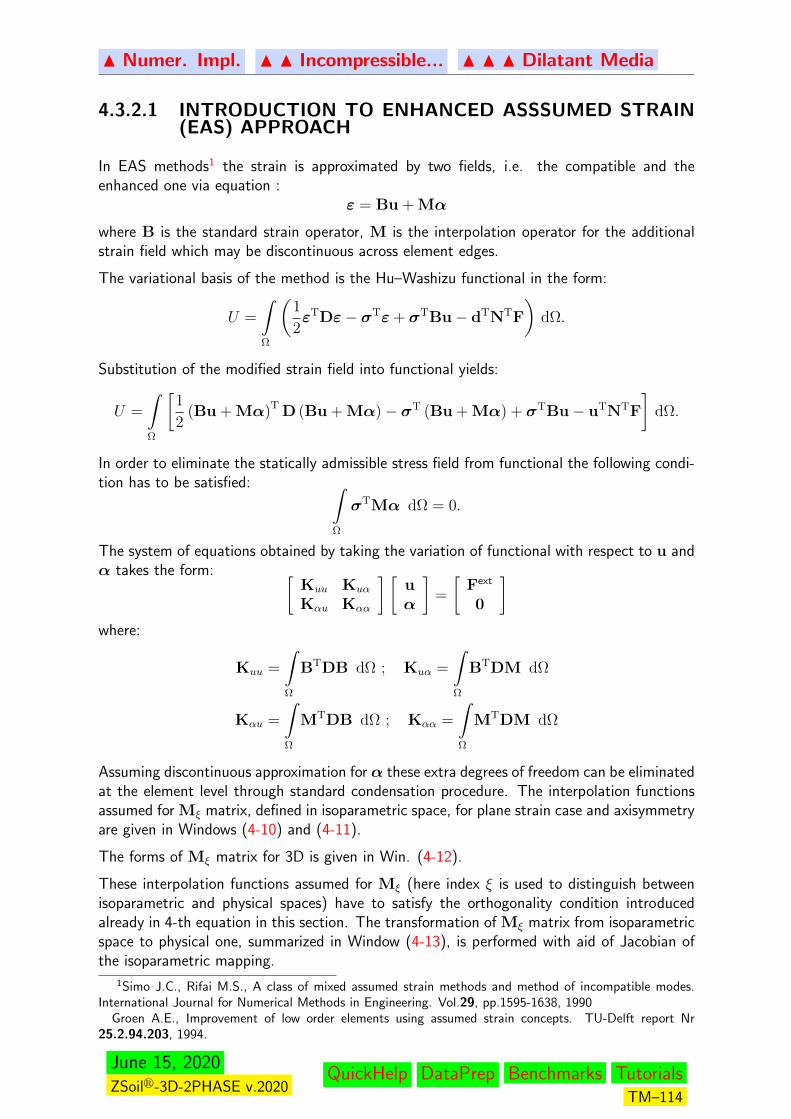
N Numer. Impl. N N Incompressible... N N N Dilatant Media
4.3.2.1 INTRODUCTION TO ENHANCED ASSSUMED STRAIN(EAS) APPROACH
In EAS methods1 the strain is approximated by two fields, i.e. the compatible and theenhanced one via equation :
ε = Bu + Mα
where B is the standard strain operator, M is the interpolation operator for the additionalstrain field which may be discontinuous across element edges.
The variational basis of the method is the Hu–Washizu functional in the form:
U =
∫Ω
(1
2εTDε− σTε+ σTBu− dTNTF
)dΩ.
Substitution of the modified strain field into functional yields:
U =
∫Ω
[1
2(Bu + Mα)T D (Bu + Mα)− σT (Bu + Mα) + σTBu− uTNTF
]dΩ.
In order to eliminate the statically admissible stress field from functional the following condi-tion has to be satisfied: ∫
Ω
σTMα dΩ = 0.
The system of equations obtained by taking the variation of functional with respect to u andα takes the form: [
Kuu Kuα
Kαu Kαα
] [uα
]=
[Fext
0
]where:
Kuu =
∫Ω
BTDB dΩ ; Kuα =
∫Ω
BTDM dΩ
Kαu =
∫Ω
MTDB dΩ ; Kαα =
∫Ω
MTDM dΩ
Assuming discontinuous approximation for α these extra degrees of freedom can be eliminatedat the element level through standard condensation procedure. The interpolation functionsassumed for Mξ matrix, defined in isoparametric space, for plane strain case and axisymmetryare given in Windows (4-10) and (4-11).
The forms of Mξ matrix for 3D is given in Win. (4-12).
These interpolation functions assumed for Mξ (here index ξ is used to distinguish betweenisoparametric and physical spaces) have to satisfy the orthogonality condition introducedalready in 4-th equation in this section. The transformation of Mξ matrix from isoparametricspace to physical one, summarized in Window (4-13), is performed with aid of Jacobian ofthe isoparametric mapping.
1Simo J.C., Rifai M.S., A class of mixed assumed strain methods and method of incompatible modes.International Journal for Numerical Methods in Engineering. Vol.29, pp.1595-1638, 1990
Groen A.E., Improvement of low order elements using assumed strain concepts. TU-Delft report Nr25.2.94.203, 1994.
June 15, 2020ZSoilr-3D-2PHASE v.2020
QuickHelp DataPrep Benchmarks TutorialsTM–114
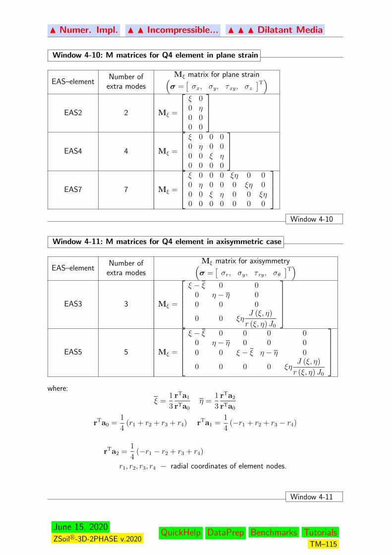
N Numer. Impl. N N Incompressible... N N N Dilatant Media
Window 4-10: M matrices for Q4 element in plane strain
EAS–elementNumber of
extra modes
Mξ matrix for plane strain(σ =
[σx, σy, τxy, σz
]T)EAS2 2 Mξ =
ξ 00 η0 00 0
EAS4 4 Mξ =
ξ 0 0 00 η 0 00 0 ξ η0 0 0 0
EAS7 7 Mξ =
ξ 0 0 0 ξη 0 00 η 0 0 0 ξη 00 0 ξ η 0 0 ξη0 0 0 0 0 0 0
Window 4-10
Window 4-11: M matrices for Q4 element in axisymmetric case
EAS–elementNumber of
extra modes
Mξ matrix for axisymmetry(σ =
[σr, σy, τ ry, σθ
]T)
EAS3 3 Mξ =
ξ − ξ 0 0
0 η − η 00 0 0
0 0 ξηJ (ξ, η)
r (ξ, η) J0
EAS5 5 Mξ =
ξ − ξ 0 0 0 0
0 η − η 0 0 0
0 0 ξ − ξ η − η 0
0 0 0 0 ξηJ (ξ, η)
r (ξ, η) J0
where:
ξ =1
3
rTa1
rTa0
η =1
3
rTa2
rTa0
rTa0 =1
4(r1 + r2 + r3 + r4) rTa1 =
1
4(−r1 + r2 + r3 − r4)
rTa2 =1
4(−r1 − r2 + r3 + r4)
r1, r2, r3, r4 − radial coordinates of element nodes.
Window 4-11
June 15, 2020ZSoilr-3D-2PHASE v.2020
QuickHelp DataPrep Benchmarks TutorialsTM–115
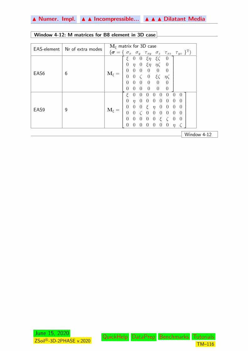
N Numer. Impl. N N Incompressible... N N N Dilatant Media
Window 4-12: M matrices for B8 element in 3D case
EAS-element Nr of extra modesMξ matrix for 3D case(σ = σx σy τxy σz τxz τ yz T)
EAS6 6 Mξ =
ξ 0 0 ξη ξζ 00 η 0 ξη ηζ 00 0 0 0 0 00 0 ζ 0 ξζ ηζ0 0 0 0 0 00 0 0 0 0 0
EAS9 9 Mξ =
ξ 0 0 0 0 0 0 0 00 η 0 0 0 0 0 0 00 0 0 ξ η 0 0 0 00 0 ζ 0 0 0 0 0 00 0 0 0 0 ξ ζ 0 00 0 0 0 0 0 0 η ζ
Window 4-12
June 15, 2020ZSoilr-3D-2PHASE v.2020
QuickHelp DataPrep Benchmarks TutorialsTM–116
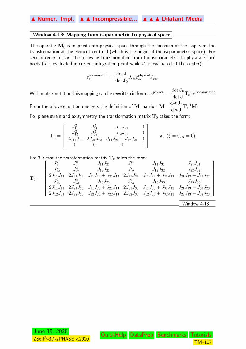
N Numer. Impl. N N Incompressible... N N N Dilatant Media
Window 4-13: Mapping from isoparametric to physical space
The operator Mξ is mapped onto physical space through the Jacobian of the isoparametrictransformation at the element centroid (which is the origin of the isoparametric space). Forsecond order tensors the following transformation from the isoparametric to physical spaceholds (J is evaluated in current integration point while J0 is evaluated at the center):
εisoparametricij =
det J
det J0
Jki0εphysicalkl Jjl0 .
With matrix notation this mapping can be rewritten in form : εphysical =det J0
det JT−1
0 εisoparametric.
From the above equation one gets the definition of M matrix: M =det J0
det JT−1
0 Mξ
For plane strain and axisymmetry the transformation matrix T0 takes the form:
T0 =
J2
11 J221 J11J21 0
J212 J2
22 J12J22 02J11J12 2J21J22 J11J22 + J12J21 0
0 0 0 1
at (ξ = 0, η = 0)
For 3D case the transformation matrix T0 takes the form:
T0 =
J2
11 J221 J11J21 J2
31 J11J31 J21J31
J212 J2
22 J12J22 J232 J12J32 J22J32
2J11J12 2J21J22 J11J22 + J21J12 2J31J32 J11J32 + J31J12 J21J32 + J31J22
J213 J2
23 J13J23 J233 J13J33 J23J33
2J11J13 2J21J23 J11J23 + J21J13 2J31J33 J11J33 + J31J13 J21J33 + J31J23
2J12J23 2J22J23 J12J23 + J22J13 2J32J33 J12J33 + J32J13 J22J33 + J32J23
Window 4-13
June 15, 2020ZSoilr-3D-2PHASE v.2020
QuickHelp DataPrep Benchmarks TutorialsTM–117
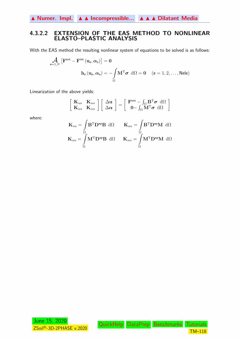
N Numer. Impl. N N Incompressible... N N N Dilatant Media
4.3.2.2 EXTENSION OF THE EAS METHOD TO NONLINEARELASTO–PLASTIC ANALYSIS
With the EAS method the resulting nonlinear system of equations to be solved is as follows:
Ae=1,N
[Fext − Fint (ue,αe)
]= 0
he (ue,αe) = −∫Ω
MTσ dΩ = 0 (e = 1, 2, . . . ,Nele)
Linearization of the above yields:[Kuu Kuα
Kαu Kαα
] [∆u∆α
]=
[Fext −
∫Ω
BTσ dΩ0−∫
ΩMTσ dΩ
]where:
Kuu =
∫Ω
BTDepB dΩ Kuα =
∫Ω
BTDepM dΩ
Kαu =
∫Ω
MTDepB dΩ Kαα =
∫Ω
MTDepM dΩ
June 15, 2020ZSoilr-3D-2PHASE v.2020
QuickHelp DataPrep Benchmarks TutorialsTM–118

N Numer. Impl. N N Incompressible... N N N Dilatant Media
4.3.2.3 REMARKS AND ASSESSMENT OF EAS ELEMENTS
1. the EAS2 element in plane strain, EAS3 in axisymmetry and EAS6 in 3D are stronglyrecommended for stability and ultimate state analysis when using isotropic plastic modelswith dilatant plastic (for ex. Drucker-Prager if ψ > 0)
2. the EAS4 element in plane strain, EAS5 in axisymmetry and EAS9 in 3D are stronglyrecommended for stability and ultimate state analysis when using anisotropic plastic modelswith any type of plastic flow (only multilaminate model)
3. if one wants to get highly accurate results for beams/shells modeled with aid of continuumelements (retaining walls, etc... ) the Q4-EAS7 (for plane strain case exclusively) andB8-EAS15 (3D) elements give superior results even for coarse distorted meshes, but theirapplication is limited to elastic type of materials only (these elements are activated onceContinuum for structures instead of Continuum is used for Material formulation
to be defined at the material level).
June 15, 2020ZSoilr-3D-2PHASE v.2020
QuickHelp DataPrep Benchmarks TutorialsTM–119

N Preface N N Numerical Implementation
4.4 FAR FIELD
Standard finite elements can be used only to discretize a bounded domain. In the case ofa problem given in an unbounded domain, infinite elements, attached to the boundary ofa bounded domain, can be used to describe interaction between bounded domain and itsinfinite surroundings. The formulation is based on the concept of infinite mapped elements(see 2). The infinite mapped elements concept is summarized in the following windows.
Formulation of the mapped infinite element
Mapping for 2D infinite element
Mapping for 3D brick type of infinite element
Mapping for 3D wedge type of infinite element
Evaluation of element matrices for infinite mapped elements
2O.C. Zienkiewicz, C. Emson, P. Bettes, A Novel Boundary Infinite Element, International Journal forNumerical Methods in Engineering, vol. 19, p.393-404, 1983
June 15, 2020ZSoilr-3D-2PHASE v.2020
QuickHelp DataPrep Benchmarks TutorialsTM–120
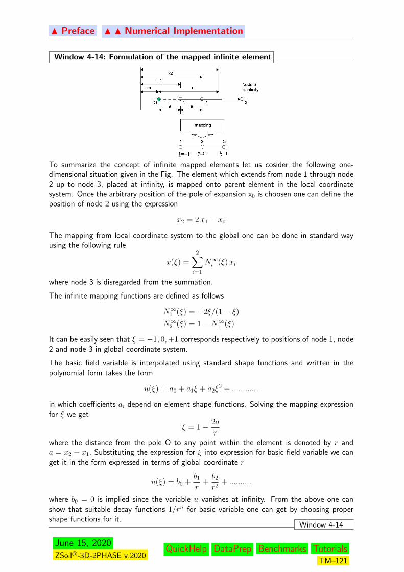
N Preface N N Numerical Implementation
Window 4-14: Formulation of the mapped infinite element
To summarize the concept of infinite mapped elements let us cosider the following one-dimensional situation given in the Fig. The element which extends from node 1 through node2 up to node 3, placed at infinity, is mapped onto parent element in the local coordinatesystem. Once the arbitrary position of the pole of expansion x0 is choosen one can define theposition of node 2 using the expression
x2 = 2x1 − x0
The mapping from local coordinate system to the global one can be done in standard wayusing the following rule
x(ξ) =2∑i=1
N∞i (ξ)xi
where node 3 is disregarded from the summation.
The infinite mapping functions are defined as follows
N∞1 (ξ) = −2ξ/(1− ξ)N∞2 (ξ) = 1−N∞1 (ξ)
It can be easily seen that ξ = −1, 0,+1 corresponds respectively to positions of node 1, node2 and node 3 in global coordinate system.
The basic field variable is interpolated using standard shape functions and written in thepolynomial form takes the form
u(ξ) = a0 + a1ξ + a2ξ2 + ............
in which coefficients ai depend on element shape functions. Solving the mapping expressionfor ξ we get
ξ = 1− 2a
rwhere the distance from the pole O to any point within the element is denoted by r anda = x2 − x1. Substituting the expression for ξ into expression for basic field variable we canget it in the form expressed in terms of global coordinate r
u(ξ) = b0 +b1
r+b2
r2+ ..........
where b0 = 0 is implied since the variable u vanishes at infinity. From the above one canshow that suitable decay functions 1/rn for basic variable one can get by choosing propershape functions for it.
Window 4-14
June 15, 2020ZSoilr-3D-2PHASE v.2020
QuickHelp DataPrep Benchmarks TutorialsTM–121
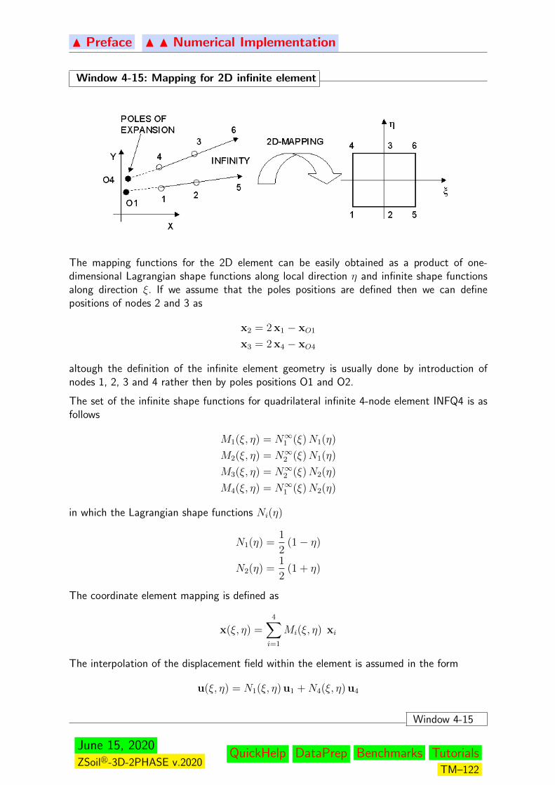
N Preface N N Numerical Implementation
Window 4-15: Mapping for 2D infinite element
The mapping functions for the 2D element can be easily obtained as a product of one-dimensional Lagrangian shape functions along local direction η and infinite shape functionsalong direction ξ. If we assume that the poles positions are defined then we can definepositions of nodes 2 and 3 as
x2 = 2 x1 − xO1
x3 = 2 x4 − xO4
altough the definition of the infinite element geometry is usually done by introduction ofnodes 1, 2, 3 and 4 rather then by poles positions O1 and O2.
The set of the infinite shape functions for quadrilateral infinite 4-node element INFQ4 is asfollows
M1(ξ, η) = N∞1 (ξ)N1(η)
M2(ξ, η) = N∞2 (ξ)N1(η)
M3(ξ, η) = N∞2 (ξ)N2(η)
M4(ξ, η) = N∞1 (ξ)N2(η)
in which the Lagrangian shape functions Ni(η)
N1(η) =1
2(1− η)
N2(η) =1
2(1 + η)
The coordinate element mapping is defined as
x(ξ, η) =4∑i=1
Mi(ξ, η) xi
The interpolation of the displacement field within the element is assumed in the form
u(ξ, η) = N1(ξ, η) u1 +N4(ξ, η) u4
Window 4-15
June 15, 2020ZSoilr-3D-2PHASE v.2020
QuickHelp DataPrep Benchmarks TutorialsTM–122
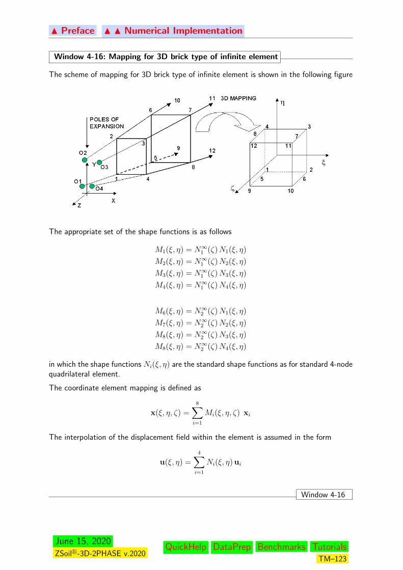
N Preface N N Numerical Implementation
Window 4-16: Mapping for 3D brick type of infinite element
The scheme of mapping for 3D brick type of infinite element is shown in the following figure
The appropriate set of the shape functions is as follows
M1(ξ, η) = N∞1 (ζ)N1(ξ, η)
M2(ξ, η) = N∞1 (ζ)N2(ξ, η)
M3(ξ, η) = N∞1 (ζ)N3(ξ, η)
M4(ξ, η) = N∞1 (ζ)N4(ξ, η)
M6(ξ, η) = N∞2 (ζ)N1(ξ, η)
M7(ξ, η) = N∞2 (ζ)N2(ξ, η)
M8(ξ, η) = N∞2 (ζ)N3(ξ, η)
M8(ξ, η) = N∞2 (ζ)N4(ξ, η)
in which the shape functions Ni(ξ, η) are the standard shape functions as for standard 4-nodequadrilateral element.
The coordinate element mapping is defined as
x(ξ, η, ζ) =8∑i=1
Mi(ξ, η, ζ) xi
The interpolation of the displacement field within the element is assumed in the form
u(ξ, η) =4∑i=1
Ni(ξ, η) ui
Window 4-16
June 15, 2020ZSoilr-3D-2PHASE v.2020
QuickHelp DataPrep Benchmarks TutorialsTM–123
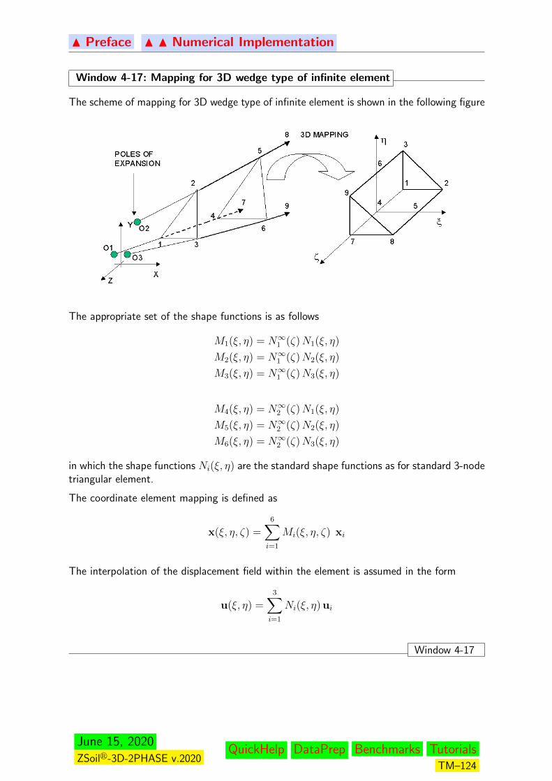
N Preface N N Numerical Implementation
Window 4-17: Mapping for 3D wedge type of infinite element
The scheme of mapping for 3D wedge type of infinite element is shown in the following figure
The appropriate set of the shape functions is as follows
M1(ξ, η) = N∞1 (ζ)N1(ξ, η)
M2(ξ, η) = N∞1 (ζ)N2(ξ, η)
M3(ξ, η) = N∞1 (ζ)N3(ξ, η)
M4(ξ, η) = N∞2 (ζ)N1(ξ, η)
M5(ξ, η) = N∞2 (ζ)N2(ξ, η)
M6(ξ, η) = N∞2 (ζ)N3(ξ, η)
in which the shape functions Ni(ξ, η) are the standard shape functions as for standard 3-nodetriangular element.
The coordinate element mapping is defined as
x(ξ, η, ζ) =6∑i=1
Mi(ξ, η, ζ) xi
The interpolation of the displacement field within the element is assumed in the form
u(ξ, η) =3∑i=1
Ni(ξ, η) ui
Window 4-17
June 15, 2020ZSoilr-3D-2PHASE v.2020
QuickHelp DataPrep Benchmarks TutorialsTM–124
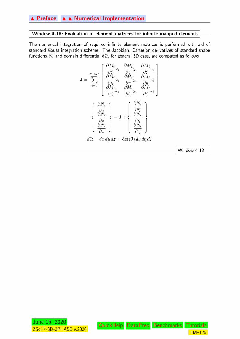
N Preface N N Numerical Implementation
Window 4-18: Evaluation of element matrices for infinite mapped elements
The numerical integration of required infinite element matrices is performed with aid ofstandard Gauss integration scheme. The Jacobian, Cartesian derivatives of standard shapefunctions Ni and domain differential dΩ, for general 3D case, are computed as follows
J =NEN∗∑i=1
∂Mi
∂ξxi
∂Mi
∂ξyi
∂Mi
∂ξzi
∂Mi
∂ηxi
∂Mi
∂ηyi
∂Mi
∂ηzi
∂Mi
∂ζxi
∂Mi
∂ζyi
∂Mi
∂ζzi
∂Ni
∂x∂Ni
∂y∂Ni
∂z
= J−1
∂Ni
∂ξ∂Ni
∂η∂Ni
∂ζ
dΩ = dx dy dz = det(J) dξ dη dζ
Window 4-18
June 15, 2020ZSoilr-3D-2PHASE v.2020
QuickHelp DataPrep Benchmarks TutorialsTM–125

N Preface N N Numerical Implementation
4.5 OVERLAID MESHES
To explain the idea of overlaid meshes let us consider a 2D domain 30m wide and 30m high,with a square excavation zone of size 6m by 6m placed at the center of the domain. Duringthe excavation a tunnel lining is installed (see Fig. below).
Tunnellining
Kinematicconstraints
q = 1 kN/m/m
In the context of the overlaid meshes approach we can create a relatively coarse mesh, labeledas layer number 0, which will represent soil behavior far from the excavation zone. In theneighborhood of the excavation zone, to enhance the quality of the results, we need a densermesh and thus we superpose a second mesh labeled as layer number 1. In the 2D casewe could easily generate a mesh in layer 1 in such a way that its external boundary nodespositions coincide with the nodes of the coarse mesh. However, in 3D applications this isusually not that easy and it is simpler, from the user’s point of view, to superpose layer 1with layer 0 without additional restrictions. This corresponds to overlaid meshes for whichwe have to handle the problem of overlapping of few meshes plus the continuity of primaryvariables (displacements, pressures etc..) handled via Lagrange multipliers.
In the considered example a mesh consisting of 10 x 10 elements is generated in layer 0 and 20x 20 elements in layer 1 (layer 1 is 14m wide and 14m high) (see Fig. above). As it is shown inFig. below some of the elements in layer 0 are fully overlapped (identified with circles) whilesome others are overlapped only partially (identified with triangles). All these elements whichare fully overlapped, and nodes which exclusively belong to these elements, are neglectedduring computations. Problems arise in the case of partially overlapped elements as partof their domain must be deleted from the resulting stiffness and right-hand-side vector. Tohandle this case an exact geometrical intersection of a given element in layer 0 and elementsin layer 1 must be computed to estimate the overlapped volume. For further application, thisintersection is computed for each integration point subdomain of a given element in layer 0and set of elements in layer 1.
June 15, 2020ZSoilr-3D-2PHASE v.2020
QuickHelp DataPrep Benchmarks TutorialsTM–126
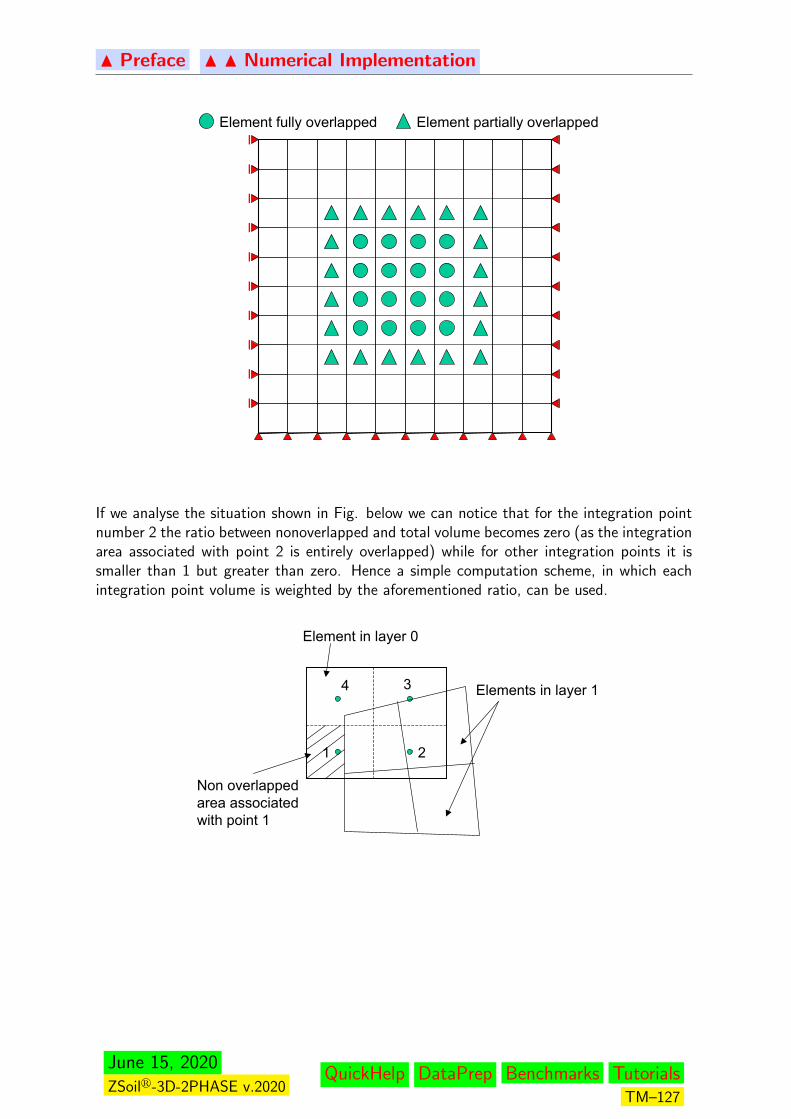
N Preface N N Numerical Implementation
Element fully overlapped Element partially overlapped
If we analyse the situation shown in Fig. below we can notice that for the integration pointnumber 2 the ratio between nonoverlapped and total volume becomes zero (as the integrationarea associated with point 2 is entirely overlapped) while for other integration points it issmaller than 1 but greater than zero. Hence a simple computation scheme, in which eachintegration point volume is weighted by the aforementioned ratio, can be used.
1 2
34
Element in layer 0
Elements in layer 1
Non overlapped area associated with point 1
June 15, 2020ZSoilr-3D-2PHASE v.2020
QuickHelp DataPrep Benchmarks TutorialsTM–127

N Preface N N Numerical Implementation
4.6 ALGORITHMS
Several solution algorithms can be activated either individually or in a sequence: initial state,stability, time dependent (driven load/consolidation/creep).
All refer in some way to a Newton–Raphson iterative scheme which is therefore described inWindow 4-19. The specific algorithms are described next.
The simulation of excavation/construction stages is managed through existence functionsassociated with elements at the level of the data preparation.
MODIFIED NEWTON-RAPHSON ALGORITHM
CONVERGENCE NORMS
INITIAL STATE ANALYSIS
STABILITY ANALYSIS
ULTIMATE LOAD ANALYSIS
CONSOLIDATION
CREEP
LOAD TIME FUNCTIONS AND TIME STEPPING
EXCAVATION AND CONSTRUCTION STAGES
June 15, 2020ZSoilr-3D-2PHASE v.2020
QuickHelp DataPrep Benchmarks TutorialsTM–128

N Preface N N Numerical Impl. N N N Algorithms
4.6.1 FULL/MODIFIED NEWTON-RAPHSON ALGORITHM
Window 4-19: Full/Modified Newton-Raphson algorithm
1. Step initialization : n = n+ 1
• set iteration counter i = 0
• set ∆u(i=0)n+1 = 0
• Accumulate total external force vector Fextn+1
2. At the element level, at each integration point
• if creep is active then compute the creep strain increment ∆εcrn+1 according to the
Section 3.4 (MATERIAL MODELS/CREEP)
• set the initial stress/strain increments ∆σ0n+1,∆ε0n+1
3. i = i+ 1
4. Assemble internal force vector and stiffness matrix using computed at the element leveland at each integration point current total stress σ
(i+1)totn+1 and current tangent stiffness
matrix Depn+1 ( an elastic stress state is computed via formula σ
(i+1)en+1 = σn + ∆σ0n+1 +
De(∆ε(i+1)n+1 −∆εcr
n+1 −∆ε0n+1) )
Fint (i+1)n+1 = A
e=1,N
∫Ωe
BTσ(i+1)totn+1 dΩ
K(i+1)n+1 = A
e=1,N
∫Ωe
BTDep(i+1)n+1 B dΩ
5. Solve system of equations
K(i+1)n+1 ∆u(i+1)=Fext
n+1 − Fint (i+1)n+1
(for modified N–R technique assume K(i+1)n+1 = Kn
(for full N–R use curent K(i+1)n+1 matrix)
6. Update accumulated increment of displacements: ∆u(i+1)n+1 = ∆u
(i)n+1 + ∆u(i+1)
7. If convergence of the iteration process has not been achieved go to step 1
Window 4-19
June 15, 2020ZSoilr-3D-2PHASE v.2020
QuickHelp DataPrep Benchmarks TutorialsTM–129
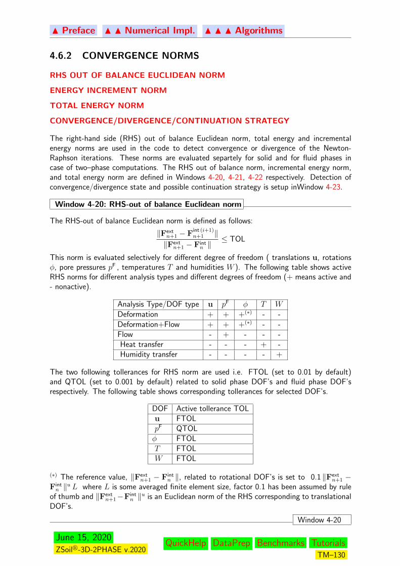
N Preface N N Numerical Impl. N N N Algorithms
4.6.2 CONVERGENCE NORMS
RHS OUT OF BALANCE EUCLIDEAN NORM
ENERGY INCREMENT NORM
TOTAL ENERGY NORM
CONVERGENCE/DIVERGENCE/CONTINUATION STRATEGY
The right-hand side (RHS) out of balance Euclidean norm, total energy and incrementalenergy norms are used in the code to detect convergence or divergence of the Newton-Raphson iterations. These norms are evaluated separtely for solid and for fluid phases incase of two–phase computations. The RHS out of balance norm, incremental energy norm,and total energy norm are defined in Windows 4-20, 4-21, 4-22 respectively. Detection ofconvergence/divergence state and possible continuation strategy is setup inWindow 4-23.
Window 4-20: RHS-out of balance Euclidean norm
The RHS-out of balance Euclidean norm is defined as follows:
‖Fextn+1 − F
int (i+1)n+1 ‖
‖Fextn+1 − Fint
n ‖≤ TOL
This norm is evaluated selectively for different degree of freedom ( translations u, rotationsφ, pore pressures pF , temperatures T and humidities W ). The following table shows activeRHS norms for different analysis types and different degrees of freedom (+ means active and- nonactive).
Analysis Type/DOF type u pF φ T W
Deformation + + +(∗) - -Deformation+Flow + + +(∗) - -Flow - + - - -Heat transfer - - - + -Humidity transfer - - - - +
The two following tollerances for RHS norm are used i.e. FTOL (set to 0.01 by default)and QTOL (set to 0.001 by default) related to solid phase DOF’s and fluid phase DOF’srespectively. The following table shows corresponding tollerances for selected DOF’s.
DOF Active tollerance TOLu FTOLpF QTOLφ FTOLT FTOLW FTOL
(∗) The reference value, ‖Fextn+1 − Fint
n ‖, related to rotational DOF’s is set to 0.1 ‖Fextn+1 −
Fintn ‖u L where L is some averaged finite element size, factor 0.1 has been assumed by rule
of thumb and ‖Fextn+1−Fint
n ‖u is an Euclidean norm of the RHS corresponding to translationalDOF’s.
Window 4-20
June 15, 2020ZSoilr-3D-2PHASE v.2020
QuickHelp DataPrep Benchmarks TutorialsTM–130
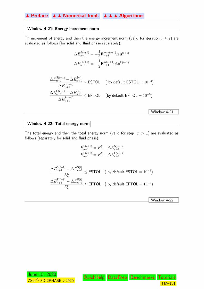
N Preface N N Numerical Impl. N N N Algorithms
Window 4-21: Energy increment norm
Th increment of energy and then the energy increment norm (valid for iteration i ≥ 2) areevaluated as follows (for solid and fluid phase separately):
∆ES(i+1)n+1 = −1
2F
intu(i+1)n+1 ∆u(i+1)
∆EF(i+1)n+1 = −1
2F
int (i+1)n+1 ∆pF (i+1)
∆ES(i+1)n+1 −∆E
S(i)n+1
∆ES(i=2)n+1
≤ ESTOL(
by default ESTOL = 10−3)
∆EF(i+1)n+1 −∆E
F(i)n+1
∆EF(i=2)n+1
≤ EFTOL(by default EFTOL = 10−3
)
Window 4-21
Window 4-22: Total energy norm
The total energy and then the total energy norm (valid for step n > 1) are evaluated asfollows (separately for solid and fluid phase):
ES(i+1)n+1 = ES
n + ∆ES(i+1)n+1
EF(i+1)n+1 = EF
n + ∆EF(i+1)n+1
∆ES(i+1)n+1 −∆E
S(i)n+1
ESn
≤ ESTOL(
by default ESTOL = 10−3)
∆EF(i+1)n+1 −∆E
F(i)n+1
EFn
≤ EFTOL(
by default EFTOL = 10−3)
Window 4-22
June 15, 2020ZSoilr-3D-2PHASE v.2020
QuickHelp DataPrep Benchmarks TutorialsTM–131
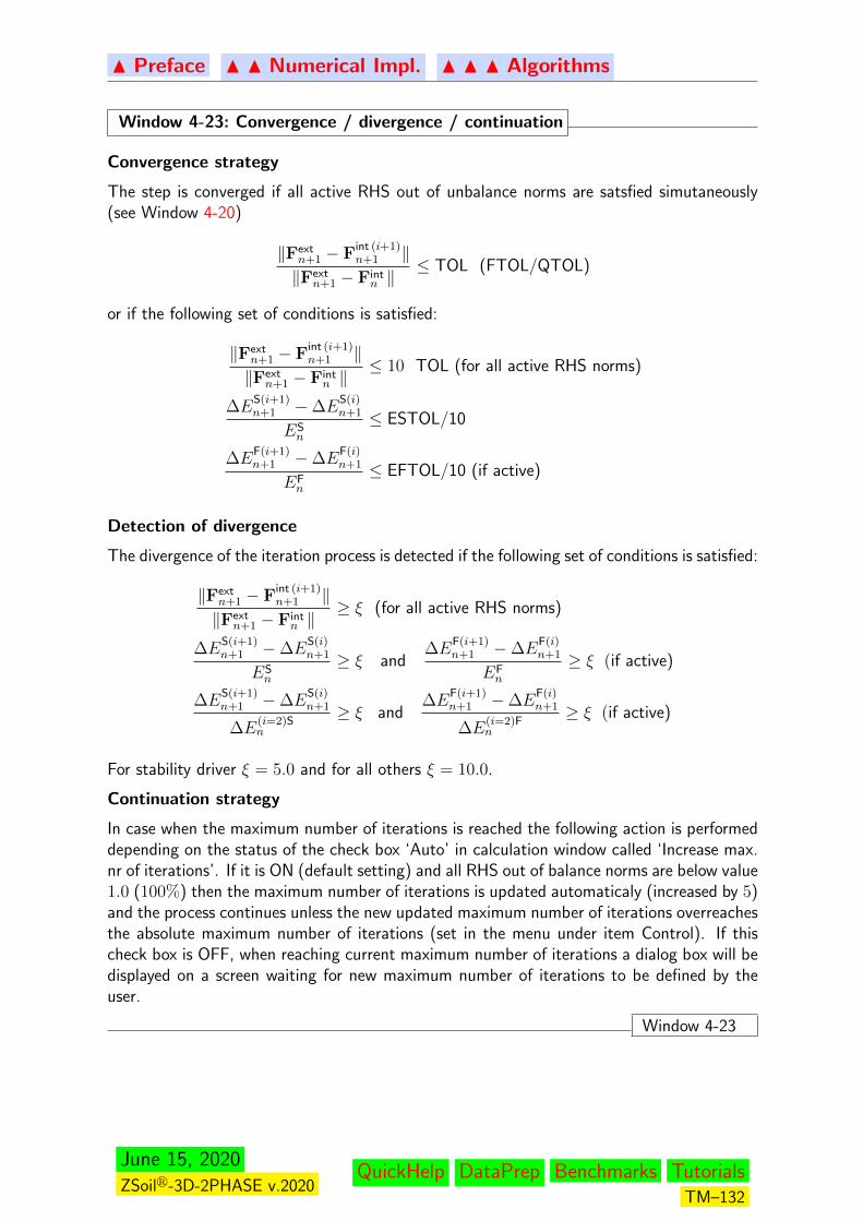
N Preface N N Numerical Impl. N N N Algorithms
Window 4-23: Convergence / divergence / continuation
Convergence strategy
The step is converged if all active RHS out of unbalance norms are satsfied simutaneously(see Window 4-20)
‖Fextn+1 − F
int (i+1)n+1 ‖
‖Fextn+1 − Fint
n ‖≤ TOL (FTOL/QTOL)
or if the following set of conditions is satisfied:
‖Fextn+1 − F
int (i+1)n+1 ‖
‖Fextn+1 − Fint
n ‖≤ 10 TOL (for all active RHS norms)
∆ES(i+1)n+1 −∆E
S(i)n+1
ESn
≤ ESTOL/10
∆EF(i+1)n+1 −∆E
F(i)n+1
EFn
≤ EFTOL/10 (if active)
Detection of divergence
The divergence of the iteration process is detected if the following set of conditions is satisfied:
‖Fextn+1 − F
int (i+1)n+1 ‖
‖Fextn+1 − Fint
n ‖≥ ξ (for all active RHS norms)
∆ES(i+1)n+1 −∆E
S(i)n+1
ESn
≥ ξ and∆E
F(i+1)n+1 −∆E
F(i)n+1
EFn
≥ ξ (if active)
∆ES(i+1)n+1 −∆E
S(i)n+1
∆E(i=2)Sn
≥ ξ and∆E
F(i+1)n+1 −∆E
F(i)n+1
∆E(i=2)Fn
≥ ξ (if active)
For stability driver ξ = 5.0 and for all others ξ = 10.0.
Continuation strategy
In case when the maximum number of iterations is reached the following action is performeddepending on the status of the check box ‘Auto’ in calculation window called ‘Increase max.nr of iterations’. If it is ON (default setting) and all RHS out of balance norms are below value1.0 (100%) then the maximum number of iterations is updated automaticaly (increased by 5)and the process continues unless the new updated maximum number of iterations overreachesthe absolute maximum number of iterations (set in the menu under item Control). If thischeck box is OFF, when reaching current maximum number of iterations a dialog box will bedisplayed on a screen waiting for new maximum number of iterations to be defined by theuser.
Window 4-23
June 15, 2020ZSoilr-3D-2PHASE v.2020
QuickHelp DataPrep Benchmarks TutorialsTM–132
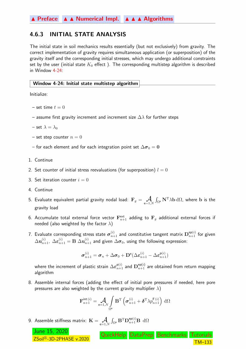
N Preface N N Numerical Impl. N N N Algorithms
4.6.3 INITIAL STATE ANALYSIS
The initial state in soil mechanics results essentially (but not exclusively) from gravity. Thecorrect implementation of gravity requires simultaneous application (or superposition) of thegravity itself and the corresponding initial stresses, which may undergo additional constraintsset by the user (initial state K0 effect ). The corresponding multistep algorithm is describedin Window 4-24:
Window 4-24: Initial state multistep algorithm
Initialize:
– set time t = 0
– assume first gravity increment and increment size ∆λ for further steps
– set λ = λ0
– set step counter n = 0
– for each element and for each integration point set ∆σ0 = 0
1. Continue
2. Set counter of initial stress reevaluations (for superposition) l = 0
3. Set iteration counter i = 0
4. Continue
5. Evaluate equivalent partial gravity nodal load: Fg = Ae=1,N
∫Ωe NTλb dΩ, where b is the
gravity load
6. Accumulate total external force vector Fextn+1 adding to Fg additional external forces if
needed (also weighted by the factor λ)
7. Evaluate corresponding stress state σ(i)n+1 and constitutive tangent matrix D
ep(i)n+1 for given
∆u(i)n+1, ∆ε
(i)n+1 = B ∆u
(i)n+1 and given ∆σ0, using the following expression:
σ(i)n+1 = σn + ∆σ0 + De(∆ε
(i)n+1 −∆ε
p(i)n+1)
where the increment of plastic strain ∆εp(i)n+1 and D
ep(i)n+1 are obtained from return mapping
algorithm
8. Assemble internal forces (adding the effect of initial pore pressures if needed, here porepressures are also weighted by the current gravity multiplier λ)
Fint (i)n+1 = A
e=1,N
∫Ωe
BT(σ
(i)n+1 + δTλp
F (i)n+1
)dΩ
9. Assemble stiffness matrix: K = Ae=1,N
∫Ωe BTD
ep(i)n+1 B dΩ
June 15, 2020ZSoilr-3D-2PHASE v.2020
QuickHelp DataPrep Benchmarks TutorialsTM–133

N Preface N N Numerical Impl. N N N Algorithms
10. Solve system of equations: K ∆u(i+1) = Fextn+1 − F
int (i)n+1
11. Update accumulated increment of displacements and strains: ∆u(i+1)n+1 = ∆u
(i)n+1 +∆u(i+1),
∆ε(i+1)n+1 = B ∆u
(i+1)n+1
12. If convergence of the iteration process has not been achieved set i = i+ 1 and go to step3
13. Increase l = l + 1
14. IF l <MAX REPEAT (by default MAX REPEAT=2) then
– Update the initial stress increment ∆σ0 (via procedure given in Window 4-25 Initialstress increment correction
– Repeat last step introducing corrected initial stresses, GO TO step 2
15. Set : ∆un+1 = ∆u(i+1)n+1 = 0, ∆εn+1 = ∆ε
(i+1)n+1 = 0
16. If n < nmax set n = n+ 1, λ = λ+ ∆λ and GO TO step 1
Window 4-24
Window 4-25: Initial stress increment correction
Correction of the assumed initial stresses is done based on the previous stress state σn,current stress state σn+1 and additional set of constraints which include the effect of K0
(the ratio between selected normal stress components can be defined in a local coordinatesystem defined by the user). We assume that the y component of the stress state is computed
accurately and we want to fulfil the conditions : σ(∗)x /σ
(∗)y = Kox and σ
(∗)z /σ
(∗)y = Koz. The
following steps lead to the evaluation of corrected initial stress increment ∆σ0.
1. Transform σn+1 → σ(∗)n+1,σn → σ
(∗)n (upper index (∗) means local system, one in which
K0 has been set up)
2. Compute stress increment between n and n+ 1 steps: ∆σ(∗)n+1 = σ
(∗)n+1 − σ
(∗)n
3. Assume : ∆σ(∗)0 = ∆σ
(∗)n+1
4. IF K0x is specified by the user then correct ∆σ(∗)0x
3: ∆σ(∗)0x = K0x ∆σ
(∗)0y
5. IF K0z is specified by the user then correct ∆σ(∗)0z : ∆σ
(∗)0z = K0z ∆σ
(∗)0y
6. Transform ∆σ(∗)0 from local K0 system to global one: ∆σ
(∗)0 → ∆σ0
Window 4-25
3Specification of K0 can be done exclusively in confined directions
June 15, 2020ZSoilr-3D-2PHASE v.2020
QuickHelp DataPrep Benchmarks TutorialsTM–134
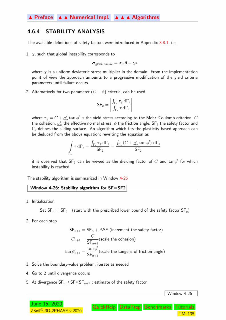
N Preface N N Numerical Impl. N N N Algorithms
4.6.4 STABILITY ANALYSIS
The available definitions of safety factors were introduced in Appendix 3.8.1, i.e.
1. χ, such that global instability corresponds to
σglobal failure = σmδ + χs
where χ is a uniform deviatoric stress multiplier in the domain. From the implementationpoint of view the approach amounts to a progressive modification of the yield criteriaparameters until failure occurs.
2. Alternatively for two-parameter (C − φ) criteria, can be used
SF2 =
∣∣∣∣∣∫
Γsτ y dΓs∫
Γsτ dΓs
∣∣∣∣∣where τ y = C + σ′n tanφ′ is the yield stress according to the Mohr–Coulomb criterion, Cthe cohesion, σ′n the effective normal stress, φ the friction angle, SF2 the safety factor andΓs defines the sliding surface. An algorithm which fits the plasticity based approach canbe deduced from the above equation; rewriting the equation as∫
Γs
τ dΓs =
∫Γsτ y dΓs
SF2
=
∫Γs
(C + σ′n tanφ′) dΓs
SF2
it is observed that SF2 can be viewed as the dividing factor of C and tanφ′ for whichinstability is reached.
The stability algorithm is summarized in Window 4-26
Window 4-26: Stability algorithm for SF=SF2
1. Initialization
Set SFn = SF0 (start with the prescribed lower bound of the safety factor SF0)
2. For each step
SFn+1 = SFn + ∆SF (increment the safety factor)
Cn+1 =C
SFn+1
(scale the cohesion)
tanφ′n+1 =tanφ′
SFn+1
(scale the tangens of friction angle)
3. Solve the boundary-value problem, iterate as needed
4. Go to 2 until divergence occurs
5. At divergence SFn ≤SF≤SFn+1 ; estimate of the safety factor
Window 4-26
June 15, 2020ZSoilr-3D-2PHASE v.2020
QuickHelp DataPrep Benchmarks TutorialsTM–135

N Preface N N Numerical Impl. N N N Algorithms
Remarks:
1. Notice that the material characteristics are modified by the algorithm, which is, strictlyspeaking, only valid ‘close’ to SF= 1.
2. Divergence is normally accompanied by a localized strain field on a slip surface, in whichSF corresponds to the given definition.
3. Let SF2 be the default definition of the safety factor for two-parameter (C − φ) criteria.
June 15, 2020ZSoilr-3D-2PHASE v.2020
QuickHelp DataPrep Benchmarks TutorialsTM–136

N Preface N N Numerical Impl. N N N Algorithms
4.6.5 ULTIMATE LOAD ANALYSIS
An ultimate load analysis follows the classical Newton–Raphson scheme. Computation arepursued until divergence is reached. Refer to Section 4.6.1. The simulation of drainedbehaviour should be done using drivers as for 1–phase or 2–phase medium but using largetime step. The undrained behavior can be done only with 2–phase algorithm (Section 4.6.6).
June 15, 2020ZSoilr-3D-2PHASE v.2020
QuickHelp DataPrep Benchmarks TutorialsTM–137
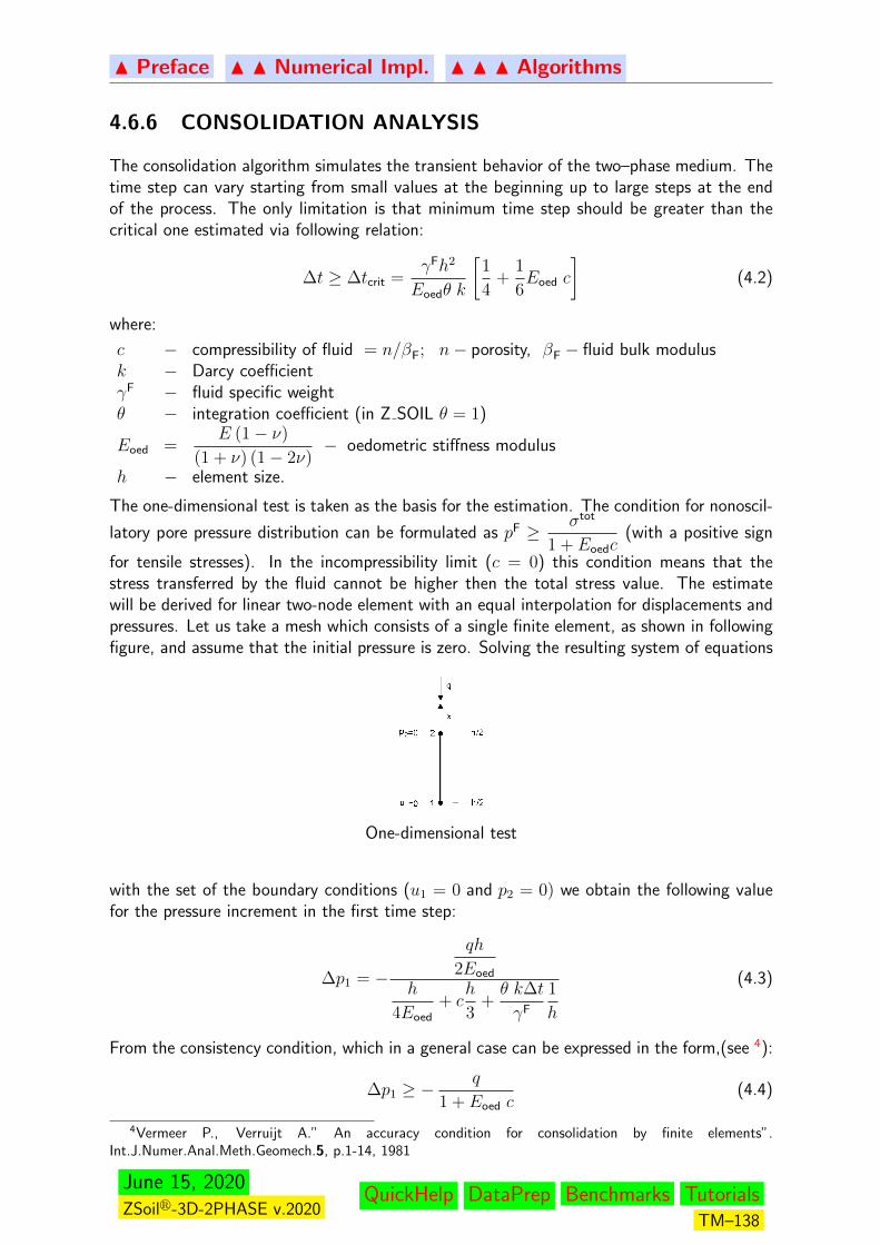
N Preface N N Numerical Impl. N N N Algorithms
4.6.6 CONSOLIDATION ANALYSIS
The consolidation algorithm simulates the transient behavior of the two–phase medium. Thetime step can vary starting from small values at the beginning up to large steps at the endof the process. The only limitation is that minimum time step should be greater than thecritical one estimated via following relation:
∆t ≥ ∆tcrit =γFh2
Eoedθ k
[1
4+
1
6Eoed c
](4.2)
where:
c − compressibility of fluid = n/βF; n− porosity, βF − fluid bulk modulusk − Darcy coefficientγF − fluid specific weightθ − integration coefficient (in Z SOIL θ = 1)
Eoed =E (1− ν)
(1 + ν) (1− 2ν)− oedometric stiffness modulus
h − element size.
The one-dimensional test is taken as the basis for the estimation. The condition for nonoscil-
latory pore pressure distribution can be formulated as pF ≥ σtot
1 + Eoedc(with a positive sign
for tensile stresses). In the incompressibility limit (c = 0) this condition means that thestress transferred by the fluid cannot be higher then the total stress value. The estimatewill be derived for linear two-node element with an equal interpolation for displacements andpressures. Let us take a mesh which consists of a single finite element, as shown in followingfigure, and assume that the initial pressure is zero. Solving the resulting system of equations
One-dimensional test
with the set of the boundary conditions (u1 = 0 and p2 = 0) we obtain the following valuefor the pressure increment in the first time step:
∆p1 = −
qh
2Eoed
h
4Eoed+ c
h
3+θ k∆t
γF
1
h
(4.3)
From the consistency condition, which in a general case can be expressed in the form,(see 4):
∆p1 ≥ −q
1 + Eoed c(4.4)
4Vermeer P., Verruijt A.” An accuracy condition for consolidation by finite elements”.Int.J.Numer.Anal.Meth.Geomech.5, p.1-14, 1981
June 15, 2020ZSoilr-3D-2PHASE v.2020
QuickHelp DataPrep Benchmarks TutorialsTM–138

N Preface N N Numerical Impl. N N N Algorithms
the condition given in eq. 4.2 for the time step ∆t is derived.
Remark:To avoid this restrictive condition the two-phase stabilization method is available inZ Soil program.
June 15, 2020ZSoilr-3D-2PHASE v.2020
QuickHelp DataPrep Benchmarks TutorialsTM–139

N Preface N N Numerical Impl. N N N Algorithms
4.6.7 CREEP ANALYSIS
Creep introduces a time dependent deformation at constant or variable stress. The imple-mentation scheme is summarized in Sect. 4.6.1. An important aspect is that the currentformulation does not produce creeping effect due to initial stresses. The phenomenon startsdue to stress variation starting at time at which the creep is activated. This means that forexample the effect of secondary consolidation understood as a result of creeping should bemodelled running the consolidation and creep simultaneously. Since creep is a time dependentprocess it requires therefore a time stepping procedure, which is shown in Window 4-27.
June 15, 2020ZSoilr-3D-2PHASE v.2020
QuickHelp DataPrep Benchmarks TutorialsTM–140

N Preface N N Numerical Impl. N N N Algorithms
4.6.8 LOAD FUNCTION AND TIME STEPPING PROCEDURE
For time dependent processes like creep, consolidation, transient flow, each item consistingload or prescribed boundary condition may have attached a function describing its variabilityin time (physical or pseudo) during the process. This is called a Load Time Function and isdefined as a list of pairs (tk, vk), as shown in Window 4-27 assuming linear interpolation for in-termediate points. Different loads acting on the model may have attached different load timefunctions, but its argument must be common for all time function in a job. It must have themeaning of a physical time (consistently with constitutive data ) for such a Time Dependent
problems as: Transient Fluid, Heat, Humidity Flow, Creep, Consolidation, while forthe remaining (i.e. Driven Load, Deformation, all Steady State) ones, may be treatedas the non-physical one.
Window 4-27: Time stepping procedure
•Load time history
Applied loads are characterized by a prescribed load amplitude and a load multiplier (loadfactor). At time tn+1 the applied load is then
Fn+1 = F0LFn+1.
The load factor LF is defined as a function of time. Each load can be associated with adifferent load factor.
Load time–history
•Time step
The time dependent processes start always with the initial time step increment defined by theuser ∆t1 = ∆tBEG. Each next time step is predicted through relation ∆tn+1 = ∆tn×∆tMULT
with time multiplier ∆tMULT defined by the user. This next time step increment can becorrected automatically by the system if in between tn ⇔ tn + ∆tpredicted
n+1 at least one of theexistence functions changes its value (from OFF to ON or vice versa) or some characteristicpoint on one of the load time functions is detected. Once such situation is detected the timestep increment is reset to the initial value ∆tBEG.
Window 4-27
June 15, 2020ZSoilr-3D-2PHASE v.2020
QuickHelp DataPrep Benchmarks TutorialsTM–141
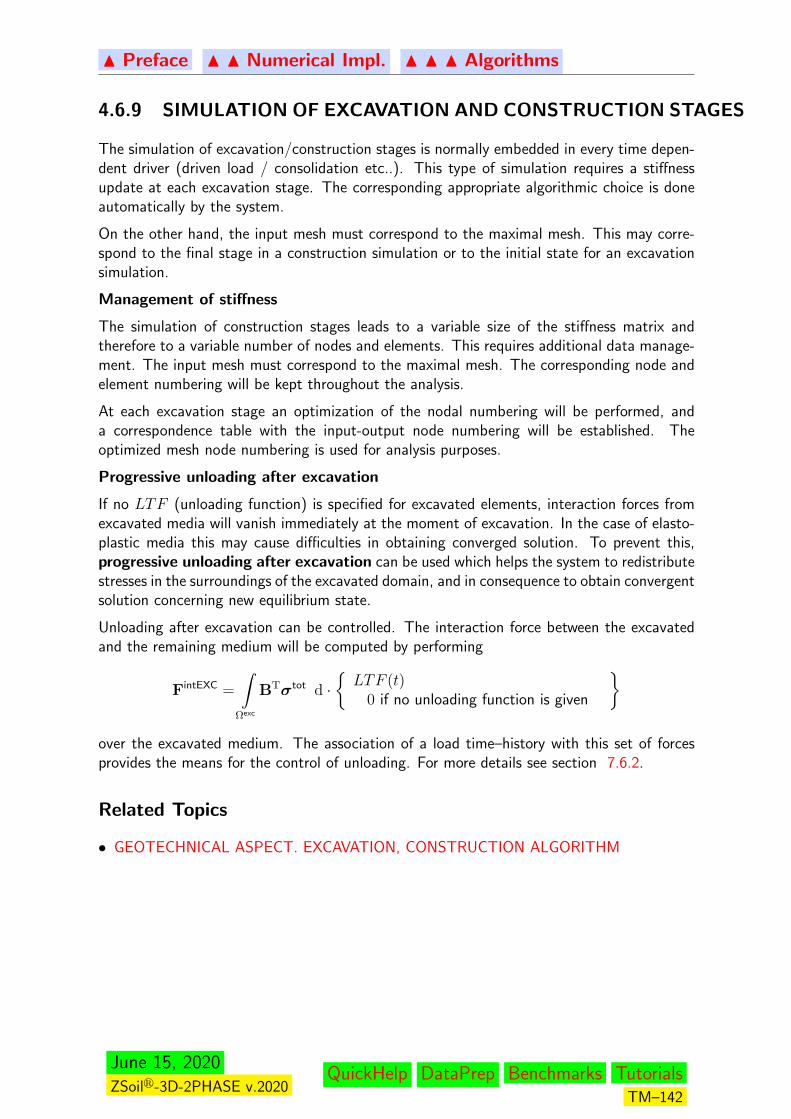
N Preface N N Numerical Impl. N N N Algorithms
4.6.9 SIMULATION OF EXCAVATION AND CONSTRUCTION STAGES
The simulation of excavation/construction stages is normally embedded in every time depen-dent driver (driven load / consolidation etc..). This type of simulation requires a stiffnessupdate at each excavation stage. The corresponding appropriate algorithmic choice is doneautomatically by the system.
On the other hand, the input mesh must correspond to the maximal mesh. This may corre-spond to the final stage in a construction simulation or to the initial state for an excavationsimulation.
Management of stiffness
The simulation of construction stages leads to a variable size of the stiffness matrix andtherefore to a variable number of nodes and elements. This requires additional data manage-ment. The input mesh must correspond to the maximal mesh. The corresponding node andelement numbering will be kept throughout the analysis.
At each excavation stage an optimization of the nodal numbering will be performed, anda correspondence table with the input-output node numbering will be established. Theoptimized mesh node numbering is used for analysis purposes.
Progressive unloading after excavation
If no LTF (unloading function) is specified for excavated elements, interaction forces fromexcavated media will vanish immediately at the moment of excavation. In the case of elasto-plastic media this may cause difficulties in obtaining converged solution. To prevent this,progressive unloading after excavation can be used which helps the system to redistributestresses in the surroundings of the excavated domain, and in consequence to obtain convergentsolution concerning new equilibrium state.
Unloading after excavation can be controlled. The interaction force between the excavatedand the remaining medium will be computed by performing
FintEXC =
∫Ωexc
BTσtot d ·LTF (t)
0 if no unloading function is given
over the excavated medium. The association of a load time–history with this set of forcesprovides the means for the control of unloading. For more details see section 7.6.2.
Related Topics
• GEOTECHNICAL ASPECT. EXCAVATION, CONSTRUCTION ALGORITHM
June 15, 2020ZSoilr-3D-2PHASE v.2020
QuickHelp DataPrep Benchmarks TutorialsTM–142

N Preface N N Numerical Implementation
4.7 APPENDICES
SHAPE FUNCTIONS AND REFERENCE ELEMENTS FOR 2D/3D
NUMERICAL INTEGRATION DATA
MULTISURFACE PLASTICITY CLOSEST POINT PROJECT ALGORITHM
SINGLE SURFACE PLASTICITY CLOSEST POINT PROJECTION ALGORITHM
June 15, 2020ZSoilr-3D-2PHASE v.2020
QuickHelp DataPrep Benchmarks TutorialsTM–143
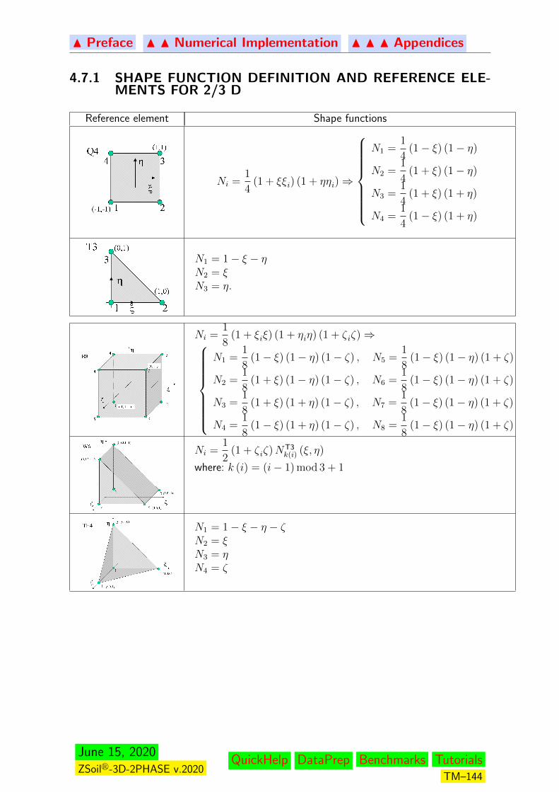
N Preface N N Numerical Implementation N N N Appendices
4.7.1 SHAPE FUNCTION DEFINITION AND REFERENCE ELE-MENTS FOR 2/3 D
Reference element Shape functions
Ni =1
4(1 + ξξi) (1 + ηηi)⇒
N1 =1
4(1− ξ) (1− η)
N2 =1
4(1 + ξ) (1− η)
N3 =1
4(1 + ξ) (1 + η)
N4 =1
4(1− ξ) (1 + η)
N1 = 1− ξ − ηN2 = ξN3 = η.
Ni =1
8(1 + ξiξ) (1 + ηiη) (1 + ζ iζ)⇒
N1 =1
8(1− ξ) (1− η) (1− ζ) , N5 =
1
8(1− ξ) (1− η) (1 + ζ)
N2 =1
8(1 + ξ) (1− η) (1− ζ) , N6 =
1
8(1− ξ) (1− η) (1 + ζ)
N3 =1
8(1 + ξ) (1 + η) (1− ζ) , N7 =
1
8(1− ξ) (1− η) (1 + ζ)
N4 =1
8(1− ξ) (1 + η) (1− ζ) , N8 =
1
8(1− ξ) (1− η) (1 + ζ)
Ni =1
2(1 + ζ iζ)NT3
k(i) (ξ, η)
where: k (i) = (i− 1) mod 3 + 1
N1 = 1− ξ − η − ζN2 = ξN3 = ηN4 = ζ
June 15, 2020ZSoilr-3D-2PHASE v.2020
QuickHelp DataPrep Benchmarks TutorialsTM–144
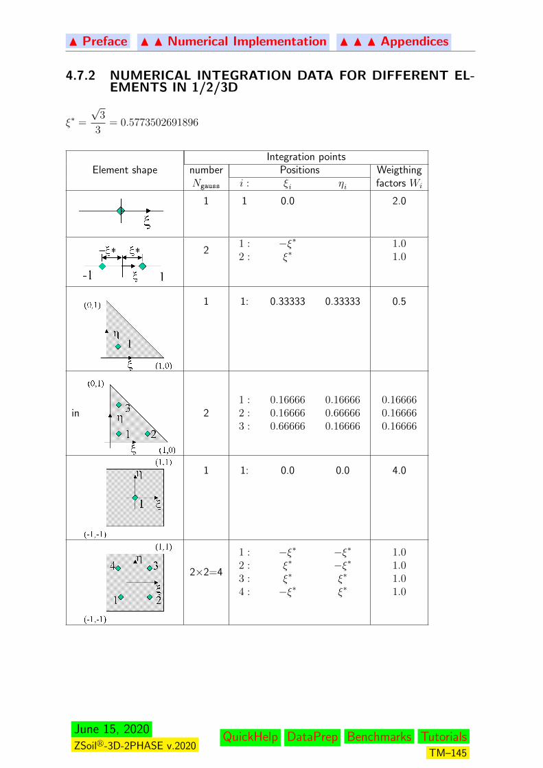
N Preface N N Numerical Implementation N N N Appendices
4.7.2 NUMERICAL INTEGRATION DATA FOR DIFFERENT EL-EMENTS IN 1/2/3D
ξ∗ =
√3
3= 0.5773502691896
Integration pointsElement shape number Positions Weigthing
Ngauss i : ξi ηi factors Wi
1 1 0.0 2.0
21 :2 :
−ξ∗ξ∗
1.01.0
1 1: 0.33333 0.33333 0.5
in 21 :2 :3 :
0.166660.166660.66666
0.166660.666660.16666
0.166660.166660.16666
1 1: 0.0 0.0 4.0
2×2=4
1 :2 :3 :4 :
−ξ∗ξ∗
ξ∗
−ξ∗
−ξ∗−ξ∗ξ∗
ξ∗
1.01.01.01.0
June 15, 2020ZSoilr-3D-2PHASE v.2020
QuickHelp DataPrep Benchmarks TutorialsTM–145
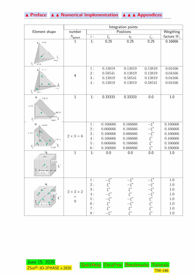
N Preface N N Numerical Implementation N N N Appendices
Integration pointsElement shape number Positions Weigthing
Ngauss i : ξi ηi ζ i factors Wi
1 1: 0.25 0.25 0.25 0.16666
4
1 :2 :3 :4 :
0.138190.585410.138190.13819
0.138190.138190.585410.13819
0.138190.138190.138190.58541
0.041660.041660.041660.04166
1 1: 0.33333 0.33333 0.0 1.0
2× 3 = 6
1 :2 :3 :4 :5 :6 :
0.1666660.6666660.1666660.1666660.6666660.166666
0.1666660.1666660.6666660.1666660.1666660.666666
−ξ∗−ξ∗−ξ∗ξ∗
ξ∗
ξ∗
0.1666660.1666660.1666660.1666660.1666660.166666
1 1: 0.0 0.0 0.0 1.0
2× 2× 2=8
1 :2 :3 :4 :5 :6 :7 :8 :
−ξ∗ξ∗
ξ∗
−ξ∗−ξ∗ξ∗
ξ∗
−ξ∗
−ξ∗−ξ∗ξ∗
ξ∗
−ξ∗−ξ∗ξ∗
ξ∗
−ξ∗−ξ∗−ξ∗−ξ∗ξ∗
ξ∗
ξ∗
ξ∗
1.01.01.01.01.01.01.01.0
June 15, 2020ZSoilr-3D-2PHASE v.2020
QuickHelp DataPrep Benchmarks TutorialsTM–146
N Preface N N Numerical Implementation N N N Appendices
4.7.3 MULTISURFACE PLASTICITY CLOSEST POINT PROJEC-TION ALGORITHM
A generalized, unconditionally stable, algorithm designed for the integration of constitutiveequations for class of multisurface elasto–plastic models is presented here. This subject hasbeen worked out first by Simo & Hughes but procedures described therein were not as generalas needed. Three crucial problems e.a.: selection of the reduced set of active mechanismssolving the plastic corrector problem in case when the number of active mechanisms is greaterthan the stress space dimension , activation of initially nonactive plastic mechanisms due toeffects of hardening/softening and finally definition of the general form of a consistent tangentmatrix for multimechanism models with generally nonassociated flow rule, and including hard-ening/softening, were introduced later by Szarlinski and Truty. Slightly modified algorithmincluding an additional substeping scheme is described here. The complete set of informationon Multisurface Closest Point Projection Stress Return Algorithm ( MCPPSS) can be foundin the following Windows:
Notation
Basic set of equations
Consistent tangent operator Dep
Window 4-28: Notation
M − number of all plastic mechanisms,Jact − actual set of active plastic mechanisms,α − mechanism index,aγ = γ∆t − plastic multiplier value,αr (σ,q) − flow vector,αh (σ,q) − column matrix of hardening/softening functions,
αq − column matrix of plastic (hardening/softening)parameters
εp − column matrix of total plastic strains,
αF − the value of plasticity condition for given stressstate and plastic parameters
D − elastic stiffness matrixC − elastic compliance matrixk − index of previous closest point projection algorithm iterationk + 1 − index of actual iterationn − index of last configuration of equilibriumn+ 1 − index of actual configuration of equilibrium
Window 4-28
Window 4-29: Set of basic equations
The integration of constitutive equations for any elasto–plastic model consists of two stagese.g. elastic predictor and plastic corrector one. Assuming the fully implicit integration scheme
June 15, 2020ZSoilr-3D-2PHASE v.2020
QuickHelp DataPrep Benchmarks TutorialsTM–147
N Preface N N Numerical Implementation N N N Appendices
for plastic strains and hardening/softening parameters this second stage is expressed by thefollowing set of equations which is the basis of the closest point projection algorithm (in thefollowing windows this will be called the basic set of equations):
εp(k+1)n+1 = εp
n +∑α=1,M
αγ(k+1)n+1
αr(k+1)n+1
q(k+1)n+1 = qn +
∑α=1,M
αγ(k+1)n+1
αh(k+1)n+1
αF(k+1)n+1 = αF
(k)n+1 + ∆ αF
(k)n+1 = 0 ∀
α∈Jact
∆σ(k+1)n+1 = −D∆ε
p(k)n+1
In most cases this system is nonlinear and Newton–Raphson procedure is needed for itssolution. To apply this procedure the consistent linerization of the above set of equationshas to be done. Denoting by Rε and Rq the residuals of the first two equations which aredefined by the following expressions:
Rε = εpn − ε
p(k)n+1 +
∑α=1,M
αγ(k)n+1
αr(k)n+1
Rq = qn − q(k)n+1 +
∑α=1,M
αγ(k)n+1
αh(k)n+1
the linearized system of first two equations of the basic set using expressions for Rε and Rq
and 4th equation from basic set is as follows (summation for ∀α∈Jact
):
(A
(k)n+1
)−1
=
[D 00 −I
]∆ε
p(k)n+1
∆q(k)n+1
=
Rε +
∑α=1,M
αγ(k)n+1
αr(k)n+1
Rq +∑α=1,M
αγ(k)n+1
αh(k)n+1
where:
A(k)n+1 =
D−1 +
∑α=1,M
αγ∂ αr(k)
∂σ
∑α=1,M
αγ∂ αr(k)
∂q∑α=1,M
αγ∂ αh(k)
∂σ
∑α=1,M
αγ∂ αh(k)
∂q− I
−1
.
In order to find increments of plastic multipliers the third equation from basic set written foreach mechanism αF : α ∈Jact has to be solved. After linearization it takes the form:
αF(k+1)n+1 =α F
(k+1)n+1 + ∆ αF
(k)n+1 =α F
(k+1)n+1 +
∂ αF(k)n+1
∂σ∆σ
(k)n+1 +
∂ αF(k)n+1
∂q∆q
(k)n+1 (1)
It can be written in matrix form using 4-th equation from basic set which leads finally to thefollowing:
αF(k)n+1 =
[∂ αF
(k)n+1
∂σD −
∂ αF(k)n+1
∂q
](2)
In the above equation vector of unknowns which consists of plastic strain and plastic variables
increments can be eliminated via expression derived for(A
(k)n+1
)−1
and finally after some
matrix manipulations this expression can be rewritten in the form:
U(k)n+1A
(k)n+1P
(k)n+1∆γ(k) = f
(k)n+1 −U
(k)n+1A
(k)n+1R
(k)n+1
June 15, 2020ZSoilr-3D-2PHASE v.2020
QuickHelp DataPrep Benchmarks TutorialsTM–148
N Preface N N Numerical Implementation N N N Appendices
where:
R(k)n+1 =
Rε
Rq
P
(k)n+1 =
[rα1 . . . rαN
hα1 . . . hαn
]
U(k)n+1 =
(∂fα1
∂σ
)T (∂fα1
∂q
)T
......(
∂fαN
∂σ
)T (∂fαN
∂q
)T
Window 4-29
Window 4-30: Consistent tangent operator Dep
The general definition of the tangent matrix is as follows:
Dep =dσ
dε.
This definition after introducing of the applied integration scheme leads to the so calledconsistent tangent matrix. The starting point for its derivation is the basic set of equationsgiven in Window 4-29 which expresses the fully implicit scheme applied for the integrationof plastic strains and plastic variables. All next steps will lead to derivation of the relationbetween dσ− dε and encapsulating from it the algorithmic constitutive operator. To do thatlet’s differentiate this basic set of equations which yields:
dεp =∑α=1,M
αγ∂ αr
∂σdσ+
∑α=1,M
αγ∂ αr
∂qdq+
∑α=1,M
α dγαr
dq =∑α=1,M
αγ∂ αh
∂σdσ+
∑α=1,M
αγ∂ αh
∂qdq+
∑α=1,M
α dγαh
d αF =∂ αF
∂σdσ+
∂ αF
∂qdq = 0; ∀
α∈Jact
dσ = D ( dε− dεp)
Considering only first two equations from the above set and eliminating the increment ofplastic strains using fourth equation we can write the following matrix equation:
C +∑α=1,M
αγ∂ αr
∂σ
∑α=1,M
αγ∂ αr
∂q∑α=1,M
αγ∂ αh
∂σ
∑α=1,M
αγ∂ αh
∂q− I
︸ ︷︷ ︸
A−1
(dσdq
)=
(dε0
)−
α∑
α=1,M
dγαr
α∑α=1,M
dγαh
Let us evaluate the stress increment considering once again the fourth equation from linearized
June 15, 2020ZSoilr-3D-2PHASE v.2020
QuickHelp DataPrep Benchmarks TutorialsTM–149
N Preface N N Numerical Implementation N N N Appendices
basic set
dσ = D ( dε− dεp) = D
( ∑α=1,M
αγ∂ αr
∂σdσ−
∑α=1,M
αγ∂ αr
∂qdq−
∑α=1,M
d αγ αr
)
= D
dε−
[ ∑α=1,M
αγ∂ αr
∂σ
∑α=1,M
αγ∂ αr
∂q
]︸ ︷︷ ︸
a
[dσdq
]−∑α=1,M
d αγ αr
.
By elimination of the plastic strain differential from the above equation we can rewrite as:
dσ = D
dε− aA
[dε0
]+ aA
∑α=1,M
d αγ αr∑α=1,M
d αγ αh
.
Let us introduce some auxiliary matrices to simplify further derivations:
– matrix r which consists of column stored flow vectors for each active mechanism r =[r1, . . . , rN ]
– vector of plastic multiplier increments: dγ =
dγ1...
dγN
– matrix K [(NSTRE+NHARD)×NSTRE] : K =
[I0
].
With these defnitions one can reform the equation for dσ:
dσ = D
dε− aA
[dε0
]+ (aAP−r) dγ
but still it is necessary to define vector dγ. It can be done writing appropriate consistencycondition for each active mechanism. Thus for all (NJACT) active mechanisms one gets thefollowing system
∂ αF
∂σ
∂ αF
∂q...
...∂ NF
∂σ
∂ NF
∂q
[
dσdq
]=
0...0
.Eliminating vector of unknowns the expression for increments of plastic multipliers will takefinally the form:
dγ = (UAP)−1 UA
[dε0
].
Introducing the above formula into the equation for dσ, after some matrix manipulations,we get the most general form of the multimechanism consistent elasto-plastic matrix:
dσ = D[I− aAK + (aAP−r) (UAP)−1 UAK
]︸ ︷︷ ︸Dep–consistent
dε.
June 15, 2020ZSoilr-3D-2PHASE v.2020
QuickHelp DataPrep Benchmarks TutorialsTM–150

N Preface N N Numerical Implementation N N N Appendices
4.7.4 SINGLE SURFACE PLASTICITY CLOSEST POINT PRO-JECTION ALGORITHM
The case of a single surface plasticity with/without hardening is handled via multisurfaceplasticity theory and algorithms assuming M=1 (nr of plastic surfaces), see Appendix 4.7.3
June 15, 2020ZSoilr-3D-2PHASE v.2020
QuickHelp DataPrep Benchmarks TutorialsTM–151

N Preface N N Numerical Implementation N N N Appendices
June 15, 2020ZSoilr-3D-2PHASE v.2020
QuickHelp DataPrep Benchmarks TutorialsTM–152

N Preface
Chapter 5
STRUCTURES
TRUSSES
BEAMS
SHELLS
MEMBRANES
APPENDICES
June 15, 2020ZSoilr-3D-2PHASE v.2020
QuickHelp DataPrep Benchmarks TutorialsTM–153

N Preface N N Structures
5.1 TRUSSES
TRUSS ELEMENT
RING ELEMENT
ANCHORING OF TRUSS AND RING ELEMENTS
PRE-STRESSING OF TRUSS AND RING ELEMENTS
UNI-AXIAL ELASTO-PLASTIC MODEL
June 15, 2020ZSoilr-3D-2PHASE v.2020
QuickHelp DataPrep Benchmarks TutorialsTM–154

N Preface N N Structures N N N Trusses
5.1.1 TRUSS ELEMENT
GENERAL IDEA OF TRUSS ELEMENT
GEOMETRY AND DOF OF TRUSS ELEMENTS
INTERPOLATION OF THE DISPLACEMENTS AND STRAINS
WEAK FORMULATION OF THE EQUILIBRIUM
STIFFNESS MATRIX AND ELEMENT FORCE VECTOR
June 15, 2020ZSoilr-3D-2PHASE v.2020
QuickHelp DataPrep Benchmarks TutorialsTM–155
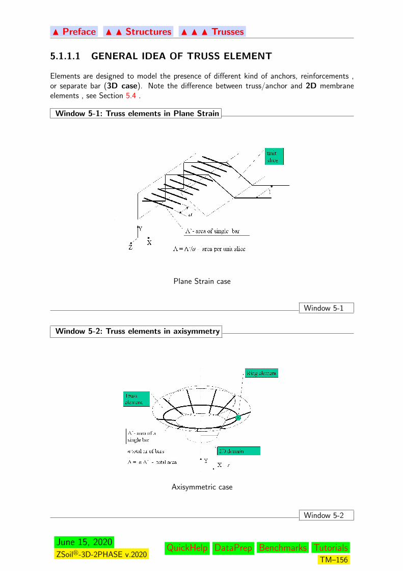
N Preface N N Structures N N N Trusses
5.1.1.1 GENERAL IDEA OF TRUSS ELEMENT
Elements are designed to model the presence of different kind of anchors, reinforcements ,or separate bar (3D case). Note the difference between truss/anchor and 2D membraneelements , see Section 5.4 .
Window 5-1: Truss elements in Plane Strain
Plane Strain case
Window 5-1
Window 5-2: Truss elements in axisymmetry
Axisymmetric case
Window 5-2
June 15, 2020ZSoilr-3D-2PHASE v.2020
QuickHelp DataPrep Benchmarks TutorialsTM–156
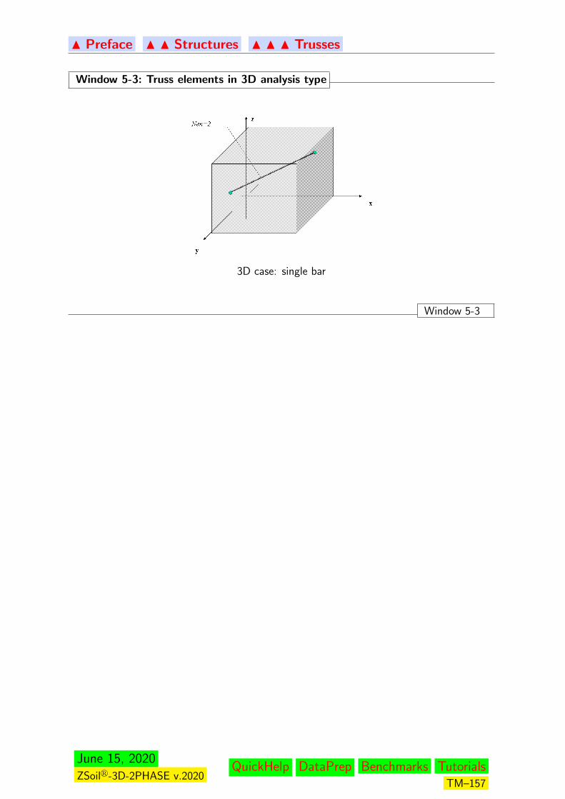
N Preface N N Structures N N N Trusses
Window 5-3: Truss elements in 3D analysis type
3D case: single bar
Window 5-3
June 15, 2020ZSoilr-3D-2PHASE v.2020
QuickHelp DataPrep Benchmarks TutorialsTM–157
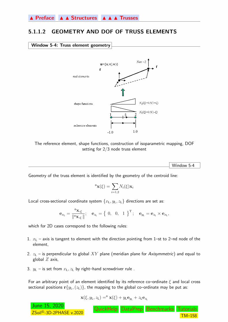
N Preface N N Structures N N N Trusses
5.1.1.2 GEOMETRY AND DOF OF TRUSS ELEMENTS
Window 5-4: Truss element geometry
The reference element, shape functions, construction of isoparametric mapping, DOFsetting for 2/3 node truss element
Window 5-4
Geometry of the truss element is identified by the geometry of the centroid line:
ox(ξ) =∑i=1,2
Ni(ξ)xi
Local cross-sectional coordinate system xL, yL, zL directions are set as:
exL=
ox,ξ‖ox,ξ ‖
; ezL=
0, 0, 1T
; eyL= ezL
× exL,
which for 2D cases correspond to the following rules:
1. xL – axis is tangent to element with the direction pointing from 1–st to 2–nd node of theelement,
2. zL – is perpendicular to global XY plane (meridian plane for Axisymmetric) and equal toglobal Z axis,
3. yL – is set from xL, zL by right–hand screwdriver rule .
For an arbitrary point of an element identified by its reference co–ordinate ξ and local crosssectional positions ryL, (zL), the mapping to the global co–ordinate may be put as:
x(ξ, yL, zL) =o x(ξ) + yLeyL+ zLezL
June 15, 2020ZSoilr-3D-2PHASE v.2020
QuickHelp DataPrep Benchmarks TutorialsTM–158
N Preface N N Structures N N N Trusses
The Jacobi matrix of the above mapping may be put as:
J =[
ox,ξ ; eyL; ezL
].
The local–global xL ↔ xG transformation matrix may be put as:
T =[
exL; eyL
; ezL
], TT =
〈exL〉
〈eyL〉
〈ezL〉
For for any vector:
vG = TvL, vL = TTvG
Evaluation of strains requires the derivatives of displacement components versus local xL axis:
v,xL= v,ξ
∂ξ
∂xL= v,ξD with D = 〈J−1〉1exL
For 2D cases a relation between local and global DOF as well as forces may be establishedin a form :
vG = TvL, vL = TTvG, with T =
[c −ss c
],
where:exL
=c, s
T, eyL
=−s, c
T
June 15, 2020ZSoilr-3D-2PHASE v.2020
QuickHelp DataPrep Benchmarks TutorialsTM–159
N Preface N N Structures N N N Trusses
5.1.1.3 INTERPOLATION OF THE DISPLACEMENTS AND STRAINS
For the point with given reference coordinate ξ translation displacement components uG
(referred to global coordinate system xG) are interpolated from its values at nodal points
uG(ξ) =∑i=1,2
Ni(ξ)uGi
The only strain component taken into account while evaluating element stress is strain alongthe element, and, as no bending is taken into account, this strain is assumed to remainconstant in the whole cross-section of the element:
εxxL(xL, yL) =
∂uL
∂xL= exL
T∂uG
∂xL,
The formulae relating the only strains component εxxLany point within the element, with its
DOF vector u may put in general for:
εxxL(ξ) = BεxL
(ξ)u =Nen∑i=1
BiεxL(ξ)ui,
For each analysis type in takes form:
• Plane Strain, Axisymmetry:
ui =[ui vi
]TBiεxL
=[exLxDNi,ξ exLyDNi,ξ
]• 3D:
ui =[ui, vi, wi
]T,
BiεxL=[exLxDNi,ξ exLyDNi,ξ exLzDNi,ξ
].
June 15, 2020ZSoilr-3D-2PHASE v.2020
QuickHelp DataPrep Benchmarks TutorialsTM–160
N Preface N N Structures N N N Trusses
5.1.1.4 WEAK FORMULATION OF THE EQUILIBRIUM
The virtual work principle expressing equilibrium of a system may be put in the general form:
find σ such that:
for any δε, δu ∫V
δεTσdV −∫∂V
δuTpd∂V = 0
The contribution of the truss elements in the above may be easily derived, with integrals takenalong the element length. A is an area attributed to the assumed computational domain i.e.to the unit slice for the Plane strain, Generalized Plane Strain , to the whole circumference(independently from current radius) for the Axisymmetric case or to one distinct bar for the3D case.
for any δε, δu ∫L
δεxxLσxxL
AdL−∫L
δuTpdL = 0
For the description of 1D uni–axial elasto–plastic material model used for truss elements seethe Window 5-29.
June 15, 2020ZSoilr-3D-2PHASE v.2020
QuickHelp DataPrep Benchmarks TutorialsTM–161
N Preface N N Structures N N N Trusses
5.1.1.5 STIFFNESS MATRIX AND ELEMENT FORCE VECTOR
Stiffness matrix Ke and force vector f e of the truss element are derived in a standard wayfrom the weak formulation of a problem. It would require constitutive module Dxxxx as wellas σxxL
stress evaluation for given strain increment. This will be performed by 1D uni–axialelasto–plastic model.
Numerical integration technique is used to evaluate integrals over the length of the element.In the case of a 2–node linear element, 1 integration point is used (Ngaus = 1, W1 = 2.0,ξ1 = 0.0). Integration over the cross section of the element is hidden in given values ofintegral characteristics of the cross section area A.
Ke =
1∫−1
BεxL
T(ξ)DxxxxBεxL(ξ)‖ox(ξ)‖dξ =
Ngaus∑igaus=1
BεxL
T(ξigaus)DxxxxBεxL(ξigaus)‖ox(ξ)‖Wigaus
f e =
1∫−1
BεxL
T(ξ)σxx(ξ)‖ox(ξ)‖dξ =
Ngaus∑igaus=1
BεxL
T(ξigaus)σxx(ξigaus)‖ox(ξigaus)‖Wigaus
The element p load is assumed to act along the centroid line leading to load induced forcesevaluated as:
fp =
1∫−1
NT(ξ)p‖ox(ξ)‖dξ =
Ngaus∑igaus=1
NT(ξigaus)p‖ox(ξigaus)‖Wigaus
where:N(ξ) =
[Ni(ξ)I(dim)
], i = 1, Nen
June 15, 2020ZSoilr-3D-2PHASE v.2020
QuickHelp DataPrep Benchmarks TutorialsTM–162

N Preface N N Structures N N N Trusses
5.1.2 RING ELEMENT
GEOMETRY AND KINEMATICS OF A RING ELEMENT
WEAK FORMULATION OF THE EQUILIBRIUM
STIFFNESS MATRIX AND ELEMENT FORCES
June 15, 2020ZSoilr-3D-2PHASE v.2020
QuickHelp DataPrep Benchmarks TutorialsTM–163
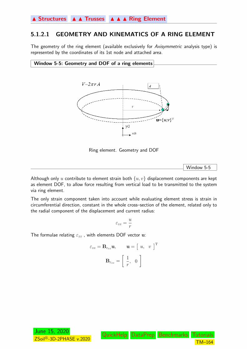
N Structures N N Trusses N N N Ring Element
5.1.2.1 GEOMETRY AND KINEMATICS OF A RING ELEMENT
The geometry of the ring element (available exclusively for Axisymmetric analysis type) isrepresented by the coordinates of its 1st node and attached area.
Window 5-5: Geometry and DOF of a ring elements
Ring element. Geometry and DOF
Window 5-5
Although only u contribute to element strain both u, v displacement components are keptas element DOF, to allow force resulting from vertical load to be transmitted to the systemvia ring element.
The only strain component taken into account while evaluating element stress is strain incircumferential direction, constant in the whole cross–section of the element, related only tothe radial component of the displacement and current radius:
εzz =u
r
The formulae relating εzz , with elements DOF vector u:
εzz = Bεzzu, u =[u, v
]TBεzz =
[1
r, 0
]
June 15, 2020ZSoilr-3D-2PHASE v.2020
QuickHelp DataPrep Benchmarks TutorialsTM–164

N Structures N N Trusses N N N Ring Element
5.1.2.2 WEAK FORMULATION OF THE EQUILIBRIUM
From the general form of the V.W.P it may be stated as:
for any δε, δu :δεzzσzz(2πrA)− δuTp(2πr) = 0
For the description of 1D uni–axial elasto–plastic material model used for ring element seethe Window 5-29
June 15, 2020ZSoilr-3D-2PHASE v.2020
QuickHelp DataPrep Benchmarks TutorialsTM–165
N Structures N N Trusses N N N Ring Element
5.1.2.3 STIFFNESS MATRIX AND ELEMENT FORCES
Stiffness matrix Ke and force vector f e of the truss element is derived in a standard wayfrom the weak formulation of a problem. It would require constitutive module Dzzzz as wellas σzz stress evaluation for given strain increment. This will be performed by 1D uni–axialelasto–plastic model, see the Window 5-29
Ke = BTεzzDzzzzBεzz2πrA
f e = BTεzzσzz2πrA
June 15, 2020ZSoilr-3D-2PHASE v.2020
QuickHelp DataPrep Benchmarks TutorialsTM–166

N Preface N N Structures N N N Trusses
5.1.3 ANCHORING OF TRUSS AND RING ELEMENTS
For the sake of generality the nodal points of truss elements may be placed in arbitraryposition within the domain occupied by continuum or structural element. Despite modelingconvenience, the option also possesses some physical meaning as then the truss elementforce are distributed over surrounding nodes of continuum element and the effect of forceconcentration is diminished.
Window 5-6: Anchoring of truss and ring elements
Conditions to be fulfilled:
• displacement compatibility:uTruss = uCont
• force equivalence (weak form):
for any δu :
δuTTrussfTruss =
Nen∑i=1
δu(i)TContf
(i)Cont
Anchoring of a truss/ring node within continuum element
Window 5-6
June 15, 2020ZSoilr-3D-2PHASE v.2020
QuickHelp DataPrep Benchmarks TutorialsTM–167
N Structures N N Trusses N N N Anchoring ...
5.1.3.1 NUMERICAL REALIZATION OF ANCHORING
Let Ni are shape functions of the element in which k–th node of a truss is anchored, and ξ∗
are local coordinates of the anchorage point within its reference element. Displacement of atruss node uTruss are to be evaluated from displacement of surrounding element uCont viacompatibility condition :
uTruss = uCont(ξ∗) =
NenCont∑i=1
Ni(ξ∗)uiCont = NTuCont
where:N = [Ni(ξ
∗)INdm] , i = 1, NenCont
In the case of anchoring within structural (i.e. beam or shell element), shape function matrixN must be understood in more general sense i.e. as a matrix relating translation displacementat arbitrary point within the element with all its DOF and takes the form given in point 1.2,1.3.
In turn, forces evaluated at the node of a truss fTruss are transferred to the nodes of thesurrounding element as fCont basing on (weakly formulated) equivalency
for any δu :
δuTTrussfTruss =
Nen∑i=1
δu(i)TContf
(i)Cont = δuContfCont ⇒
δuTTrussfTruss = δuT
ContNfCont = δuContfCont ⇒ fCont = NfTruss
Finally, the stiffness of the truss element is assembled on the DOF of surrounding element,and takes a form as bellow, where Kjk are j–th and k–th nodal sub–matrix of the trussstiffness:
K =
Kjj... KjkN
T
s s s
NKkj... NKkkN
T
In the case of the ring element, its stiffness assembled on the DOF of surrounding elementstakes form:
K = NKkkNT.
June 15, 2020ZSoilr-3D-2PHASE v.2020
QuickHelp DataPrep Benchmarks TutorialsTM–168
N Preface N N Structures N N N Trusses
5.1.4 PRE–STRESSING OF TRUSS AND RING ELEMENTS
Pre-stress can be applied only to anchor/truss or ring elements. Pre–stress differs from astandard initial stress situation by the fact, that the internal force is assumed to be known apriori. According to the definition of current tangent stiffness matrix it follows that:
K =∂f(u)
∂u= 0
since internal force f(u) is constant. As a consequence, if pre-stress is being applied thenthe stiffness of the anchor is always set to zero while it is evaluated via standard proceduresif pre- stress is non–active.
Strains in the anchor / ring element are monitored during the pre-stress as:
εi = εi−1 + ∆εi
∆εi =σprestres(ti)− σi−1
E
June 15, 2020ZSoilr-3D-2PHASE v.2020
QuickHelp DataPrep Benchmarks TutorialsTM–169

N Preface N N Structures
5.2 BEAMS
GEOMETRY OF BEAM ELEMENT
KINEMATICS OF BEAM THEORY
WEAK FORMULATION OF THE EQUILIBRIUM
INTERPOLATION OF THE DISPLACEMENT FIELD
STRAIN REPRESENTATION
STIFFNESS MATRIX AND ELEMENT FORCES
MASTER-CENTROID (OFFSET) TRANSFORMATION
RELAXATION OF INTERNAL DOF
BEAM ELEMENT RESULTS
June 15, 2020ZSoilr-3D-2PHASE v.2020
QuickHelp DataPrep Benchmarks TutorialsTM–170
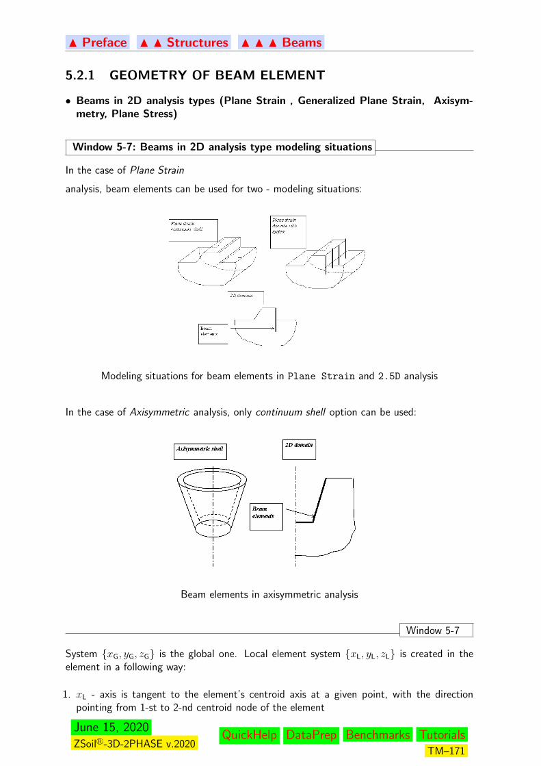
N Preface N N Structures N N N Beams
5.2.1 GEOMETRY OF BEAM ELEMENT
• Beams in 2D analysis types (Plane Strain , Generalized Plane Strain, Axisym-metry, Plane Stress)
Window 5-7: Beams in 2D analysis type modeling situations
In the case of Plane Strain
analysis, beam elements can be used for two - modeling situations:
Modeling situations for beam elements in Plane Strain and 2.5D analysis
In the case of Axisymmetric analysis, only continuum shell option can be used:
Beam elements in axisymmetric analysis
Window 5-7
System xG, yG, zG is the global one. Local element system xL, yL, zL is created in theelement in a following way:
1. xL - axis is tangent to the element’s centroid axis at a given point, with the directionpointing from 1-st to 2-nd centroid node of the element
June 15, 2020ZSoilr-3D-2PHASE v.2020
QuickHelp DataPrep Benchmarks TutorialsTM–171
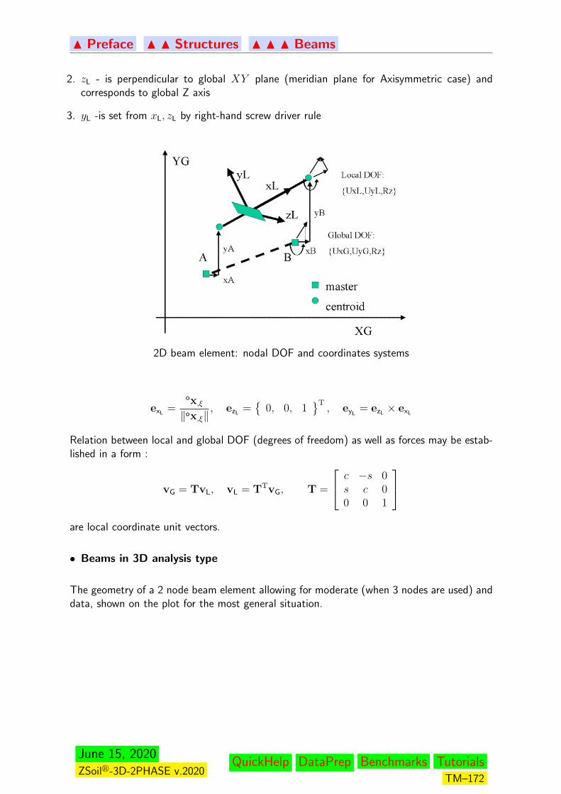
N Preface N N Structures N N N Beams
2. zL - is perpendicular to global XY plane (meridian plane for Axisymmetric case) andcorresponds to global Z axis
3. yL -is set from xL, zL by right-hand screw driver rule
2D beam element: nodal DOF and coordinates systems
exL=
ox,ξ‖ox,ξ‖
, ezL=
0, 0, 1T
, eyL= ezL
× exL
Relation between local and global DOF (degrees of freedom) as well as forces may be estab-lished in a form :
vG = TvL, vL = TTvG, T =
c −s 0s c 00 0 1
are local coordinate unit vectors.
• Beams in 3D analysis type
The geometry of a 2 node beam element allowing for moderate (when 3 nodes are used) anddata, shown on the plot for the most general situation.
June 15, 2020ZSoilr-3D-2PHASE v.2020
QuickHelp DataPrep Benchmarks TutorialsTM–172
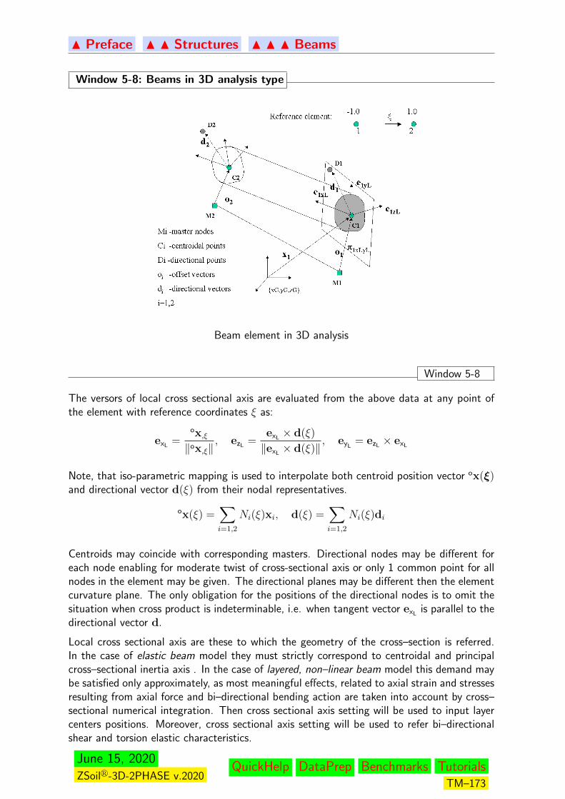
N Preface N N Structures N N N Beams
Window 5-8: Beams in 3D analysis type
Beam element in 3D analysis
Window 5-8
The versors of local cross sectional axis are evaluated from the above data at any point ofthe element with reference coordinates ξ as:
exL=
ox,ξ‖ox,ξ‖
, ezL=
exL× d(ξ)
‖exL× d(ξ)‖
, eyL= ezL
× exL
Note, that iso-parametric mapping is used to interpolate both centroid position vector ox(ξ)and directional vector d(ξ) from their nodal representatives.
ox(ξ) =∑i=1,2
Ni(ξ)xi, d(ξ) =∑i=1,2
Ni(ξ)di
Centroids may coincide with corresponding masters. Directional nodes may be different foreach node enabling for moderate twist of cross-sectional axis or only 1 common point for allnodes in the element may be given. The directional planes may be different then the elementcurvature plane. The only obligation for the positions of the directional nodes is to omit thesituation when cross product is indeterminable, i.e. when tangent vector exL
is parallel to thedirectional vector d.
Local cross sectional axis are these to which the geometry of the cross–section is referred.In the case of elastic beam model they must strictly correspond to centroidal and principalcross–sectional inertia axis . In the case of layered, non–linear beam model this demand maybe satisfied only approximately, as most meaningful effects, related to axial strain and stressesresulting from axial force and bi–directional bending action are taken into account by cross–sectional numerical integration. Then cross sectional axis setting will be used to input layercenters positions. Moreover, cross sectional axis setting will be used to refer bi–directionalshear and torsion elastic characteristics.
June 15, 2020ZSoilr-3D-2PHASE v.2020
QuickHelp DataPrep Benchmarks TutorialsTM–173

N Preface N N Structures N N N Beams
For local cross sectional positions ryL, (zL), the mapping to the global co–ordinate may beput as:
x(ξ, yL, zL) = ox(ξ) + yLeyL+ zLezL
The Jacobi matrix of the above mapping may be put as:
J(ξ, yL, zL) =[
ox,ξ + yLeyL,ξ +zLezL
,ξ ; eyL; ezL
]The local-global xL ↔ xG transformation matrix may be put as:
T =[
exL; eyL
; ezL
], TT =
〈exL〉
〈eyL〉
〈ezL〉
thus for any vector :
vG = TvL,vL = TTvG.
Evaluation of strains requires the derivatives of any displacement components versus local xLaxis :
v,xL= v,ξ
∂ξ
∂xL= v,ξD with D = 〈J−1〉1exL
In 3D analysis case ξ–derivatives of base vectors eL appear, evaluated as:
exL,ξ =1
‖ox,ξ‖
(I−
ox,ξ ⊗o x,ξox,ξ ·o x,ξ
)ox,ξξ
ezL=
1
‖exL× d‖
(I− (exL
× d)⊗ (exL× d)
(exL× d) · (exL
× d)
)(exL,ξ × d + exL
× d,ξ)
eyL= ezL,ξ × exL
+ ezL× exL,ξ
June 15, 2020ZSoilr-3D-2PHASE v.2020
QuickHelp DataPrep Benchmarks TutorialsTM–174
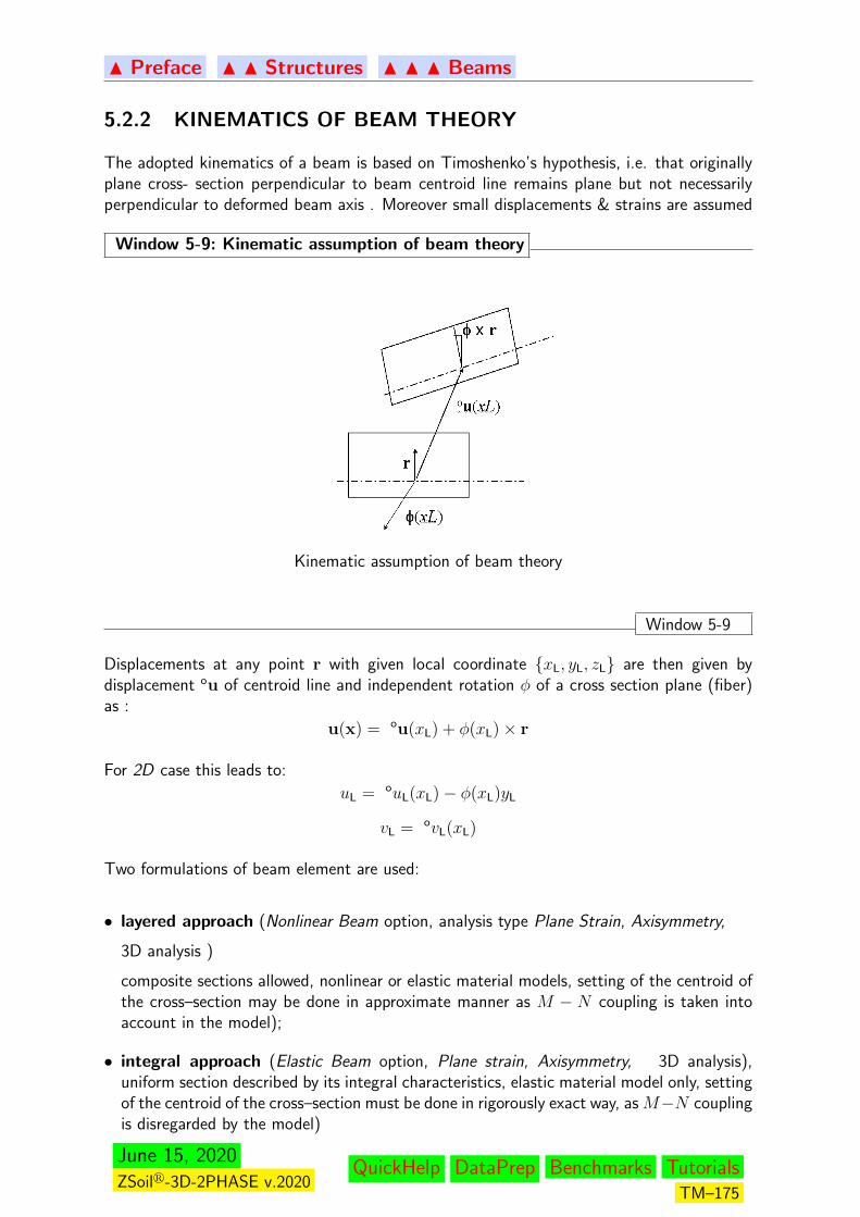
N Preface N N Structures N N N Beams
5.2.2 KINEMATICS OF BEAM THEORY
The adopted kinematics of a beam is based on Timoshenko’s hypothesis, i.e. that originallyplane cross- section perpendicular to beam centroid line remains plane but not necessarilyperpendicular to deformed beam axis . Moreover small displacements & strains are assumed
Window 5-9: Kinematic assumption of beam theory
Kinematic assumption of beam theory
Window 5-9
Displacements at any point r with given local coordinate xL, yL, zL are then given bydisplacement ou of centroid line and independent rotation φ of a cross section plane (fiber)as :
u(x) = ou(xL) + φ(xL)× r
For 2D case this leads to:
uL = ouL(xL)− φ(xL)yL
vL = ovL(xL)
Two formulations of beam element are used:
• layered approach (Nonlinear Beam option, analysis type Plane Strain, Axisymmetry,
3D analysis )
composite sections allowed, nonlinear or elastic material models, setting of the centroid ofthe cross–section may be done in approximate manner as M − N coupling is taken intoaccount in the model);
• integral approach (Elastic Beam option, Plane strain, Axisymmetry, 3D analysis),uniform section described by its integral characteristics, elastic material model only, settingof the centroid of the cross–section must be done in rigorously exact way, as M−N couplingis disregarded by the model)
June 15, 2020ZSoilr-3D-2PHASE v.2020
QuickHelp DataPrep Benchmarks TutorialsTM–175
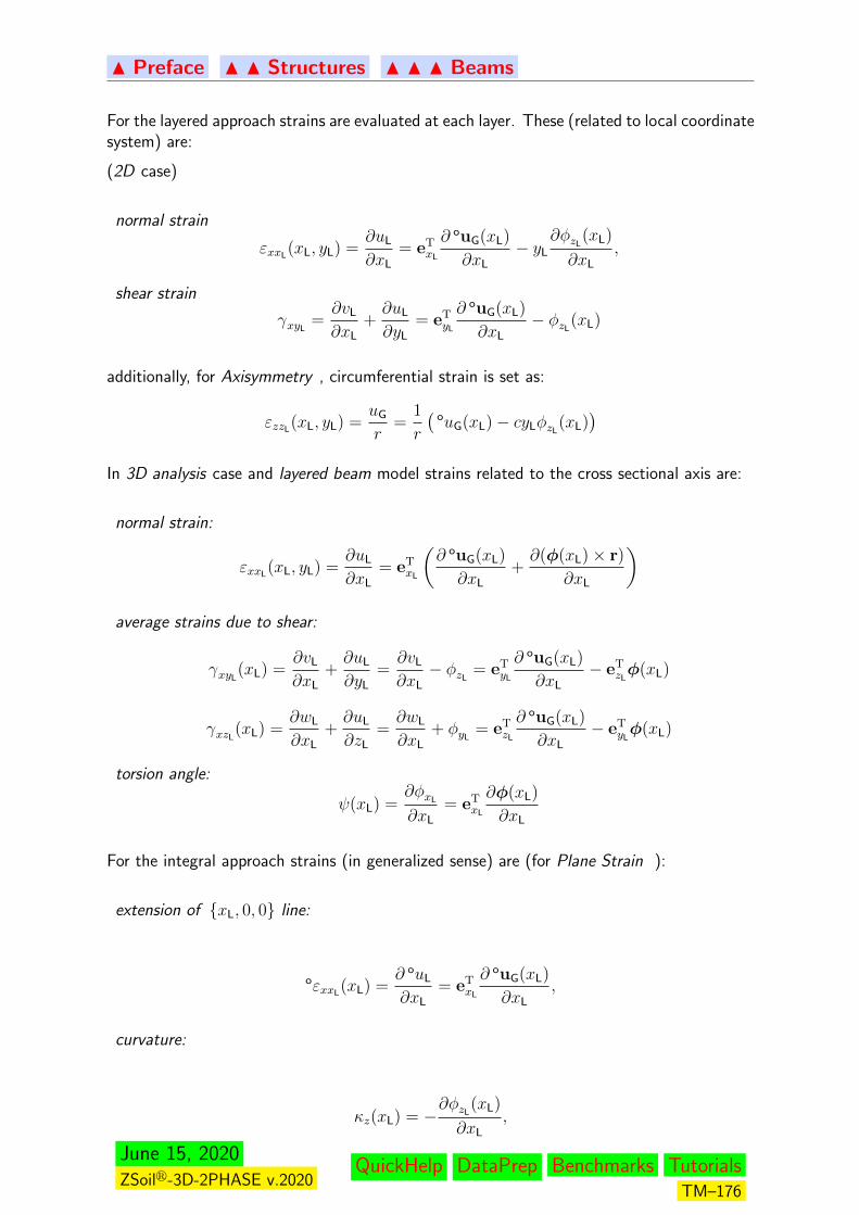
N Preface N N Structures N N N Beams
For the layered approach strains are evaluated at each layer. These (related to local coordinatesystem) are:
(2D case)
normal strain
εxxL(xL, yL) =
∂uL
∂xL= eT
xL
∂ ouG(xL)
∂xL− yL
∂φzL(xL)
∂xL,
shear strain
γxyL=∂vL
∂xL+∂uL
∂yL= eT
yL
∂ ouG(xL)
∂xL− φzL
(xL)
additionally, for Axisymmetry , circumferential strain is set as:
εzzL(xL, yL) =
uG
r=
1
r
(ouG(xL)− cyLφzL
(xL))
In 3D analysis case and layered beam model strains related to the cross sectional axis are:
normal strain:
εxxL(xL, yL) =
∂uL
∂xL= eT
xL
(∂ ouG(xL)
∂xL+∂(φ(xL)× r)
∂xL
)average strains due to shear:
γxyL(xL) =
∂vL
∂xL+∂uL
∂yL=∂vL
∂xL− φzL
= eTyL
∂ ouG(xL)
∂xL− eT
zLφ(xL)
γxzL(xL) =
∂wL
∂xL+∂uL
∂zL=∂wL
∂xL+ φyL
= eTzL
∂ ouG(xL)
∂xL− eT
yLφ(xL)
torsion angle:
ψ(xL) =∂φxL
∂xL= eT
xL
∂φ(xL)
∂xL
For the integral approach strains (in generalized sense) are (for Plane Strain ):
extension of xL, 0, 0 line:
oεxxL(xL) =
∂ ouL
∂xL= eT
xL
∂ ouG(xL)
∂xL,
curvature:
κz(xL) = −∂φzL
(xL)
∂xL,
June 15, 2020ZSoilr-3D-2PHASE v.2020
QuickHelp DataPrep Benchmarks TutorialsTM–176
N Preface N N Structures N N N Beams
average shear strain:
γxyL(xL) =
∂vL
∂xL+∂uL
∂yL= eT
yL
∂ouG(xL)
∂xL− φzL
(xL).
In 3D case (integral approach) generalized strains are:
extension of xL, 0, 0 line:
oεxxL(xL) =
∂ ouL
∂xL= eT
xL
∂ ouG(xL)
∂xL,
curvatures:
κy(xL) =∂φyL
(xL)
∂xL= eT
yL
∂φ(xL)
∂xL,
κz(xL) = −∂φzL
(xL)
∂xL= −eT
zL
∂φ(xL)
∂xL,
Also average strains due to shear and torsion angle taking the form identical as for layeredbeam are taken into account.
June 15, 2020ZSoilr-3D-2PHASE v.2020
QuickHelp DataPrep Benchmarks TutorialsTM–177
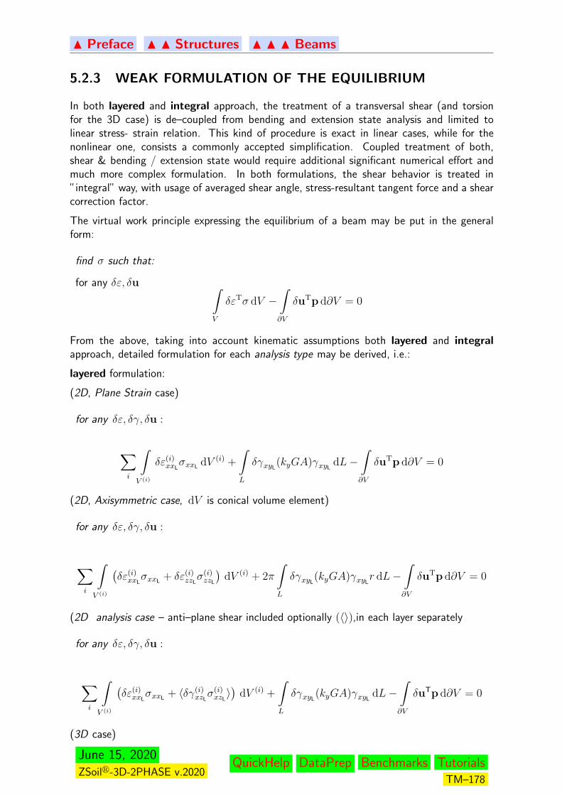
N Preface N N Structures N N N Beams
5.2.3 WEAK FORMULATION OF THE EQUILIBRIUM
In both layered and integral approach, the treatment of a transversal shear (and torsionfor the 3D case) is de–coupled from bending and extension state analysis and limited tolinear stress- strain relation. This kind of procedure is exact in linear cases, while for thenonlinear one, consists a commonly accepted simplification. Coupled treatment of both,shear & bending / extension state would require additional significant numerical effort andmuch more complex formulation. In both formulations, the shear behavior is treated in”integral” way, with usage of averaged shear angle, stress-resultant tangent force and a shearcorrection factor.
The virtual work principle expressing the equilibrium of a beam may be put in the generalform:
find σ such that:
for any δε, δu ∫V
δεTσ dV −∫∂V
δuTp d∂V = 0
From the above, taking into account kinematic assumptions both layered and integralapproach, detailed formulation for each analysis type may be derived, i.e.:
layered formulation:
(2D, Plane Strain case)
for any δε, δγ, δu :
∑i
∫V (i)
δε(i)xxLσxxL
dV (i) +
∫L
δγxyL(kyGA)γxyL
dL−∫∂V
δuTp d∂V = 0
(2D, Axisymmetric case, dV is conical volume element)
for any δε, δγ, δu :
∑i
∫V (i)
(δε(i)
xxLσxxL
+ δε(i)zzLσ(i)zzL
)dV (i) + 2π
∫L
δγxyL(kyGA)γxyL
r dL−∫∂V
δuTp d∂V = 0
(2D analysis case – anti–plane shear included optionally (〈〉),in each layer separately
for any δε, δγ, δu :
∑i
∫V (i)
(δε(i)
xxLσxxL
+ 〈δγ(i)xzLσ(i)xzL〉)
dV (i) +
∫L
δγxyL(kyGA)γxyL
dL−∫∂V
δuTp d∂V = 0
(3D case)
June 15, 2020ZSoilr-3D-2PHASE v.2020
QuickHelp DataPrep Benchmarks TutorialsTM–178
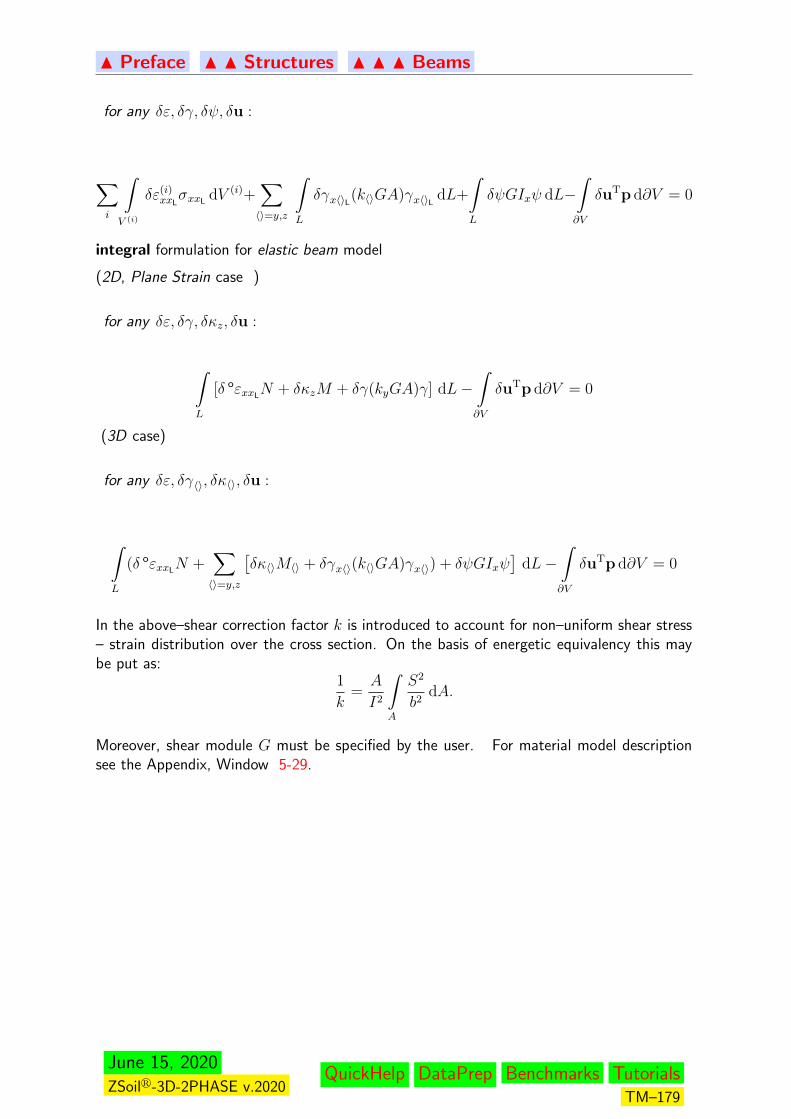
N Preface N N Structures N N N Beams
for any δε, δγ, δψ, δu :
∑i
∫V (i)
δε(i)xxLσxxL
dV (i)+∑〈〉=y,z
∫L
δγx〈〉L(k〈〉GA)γx〈〉L dL+
∫L
δψGIxψ dL−∫∂V
δuTp d∂V = 0
integral formulation for elastic beam model
(2D, Plane Strain case )
for any δε, δγ, δκz, δu :
∫L
[δ oεxxLN + δκzM + δγ(kyGA)γ] dL−
∫∂V
δuTp d∂V = 0
(3D case)
for any δε, δγ〈〉, δκ〈〉, δu :
∫L
(δ oεxxLN +
∑〈〉=y,z
[δκ〈〉M〈〉 + δγx〈〉(k〈〉GA)γx〈〉) + δψGIxψ
]dL−
∫∂V
δuTp d∂V = 0
In the above–shear correction factor k is introduced to account for non–uniform shear stress– strain distribution over the cross section. On the basis of energetic equivalency this maybe put as:
1
k=A
I2
∫A
S2
b2dA.
Moreover, shear module G must be specified by the user. For material model descriptionsee the Appendix, Window 5-29.
June 15, 2020ZSoilr-3D-2PHASE v.2020
QuickHelp DataPrep Benchmarks TutorialsTM–179

N Preface N N Structures N N N Beams
5.2.4 INTERPOLATION OF THE DISPLACEMENT FIELD
For the point lying on the element centroid line with given reference coordinate ξ, bothtranslations u and rotational φ, displacement components (referred to global coordinatesystem ) are interpolated from its values at the centroid nodes Ci. Note, that these maybe obtained from element DOF by ”master” to ”centroid” offset transformation ,see theAppendix, Window 5-26.
ouG(ξ) =∑i=1,2
Ni(ξ)uGCi
oφG(ξ) =∑i=1,2
Ni(ξ)φGCi
June 15, 2020ZSoilr-3D-2PHASE v.2020
QuickHelp DataPrep Benchmarks TutorialsTM–180

N Preface N N Structures N N N Beams
5.2.5 STRAIN REPRESENTATION
The formulae relating strains any point within the element with its DOF vector q, based onkinematic assumptions is given in general form:
ε(ξ, yL, zL) = B(ξ, yL, zL)q =Nen∑i=1
Bi(ξ, yL, zL)qi, qi =
[uCi
φCi
]
The displacement vector q consist of:
2D–Plane Strain, Axisymmetry:
qi =[u, v, φz
]T3D analysis:
qi =[u, v, w, φx, φy, φz
]Ti-th node submatrix of B-matrix relating shear strain with nodal DOF has a form in the caseof:
2D–Plane Strain, Axisymmetry:
Bγi =[eyLxDNi,ξ ; eyLyDNi,ξ ; −Ni
]
3D analysis:Bγxyi
=[DNi,ξ eT
yL; −Nie
TyL
]Bγxzi
=[DNi,ξ eT
zL; −Nie
TzL
]In that case also torsion angle matrix Bψ should be set as :
Bψi=[
01×3; DNi,ξ eTxL
]Remaining strain component one–node sub–matrix Bi takes form (for straight geometryelement):
• layered approach:
2D–Plane Strain:
axial strain
BεxLi=[exLxDNi,ξ ; exLyDNi,ξ ; −DNi,ξ yL
]2D–Axisymmetry:
axial strain:
June 15, 2020ZSoilr-3D-2PHASE v.2020
QuickHelp DataPrep Benchmarks TutorialsTM–181
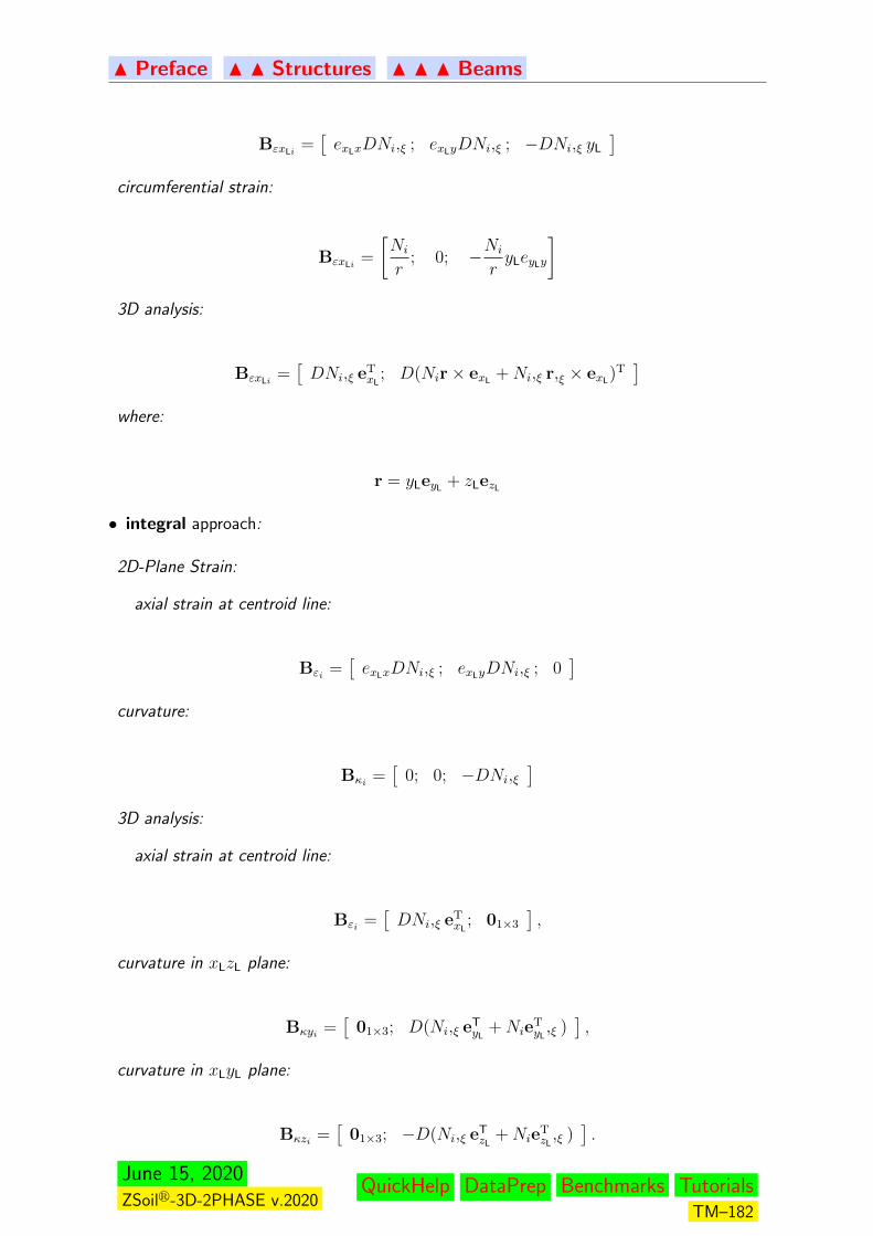
N Preface N N Structures N N N Beams
BεxLi=[exLxDNi,ξ ; exLyDNi,ξ ; −DNi,ξ yL
]circumferential strain:
BεxLi=
[Ni
r; 0; −Ni
ryLeyLy
]3D analysis:
BεxLi=[DNi,ξ eT
xL; D(Nir× exL
+Ni,ξ r,ξ × exL)T]
where:
r = yLeyL+ zLezL
• integral approach:
2D-Plane Strain:
axial strain at centroid line:
Bεi =[exLxDNi,ξ ; exLyDNi,ξ ; 0
]curvature:
Bκi =[
0; 0; −DNi,ξ]
3D analysis:
axial strain at centroid line:
Bεi =[DNi,ξ eT
xL; 01×3
],
curvature in xLzL plane:
Bκyi =[
01×3; D(Ni,ξ eTyL
+NieTyL,ξ )
],
curvature in xLyL plane:
Bκzi =[
01×3; −D(Ni,ξ eTzL
+NieTzL,ξ )
].
June 15, 2020ZSoilr-3D-2PHASE v.2020
QuickHelp DataPrep Benchmarks TutorialsTM–182
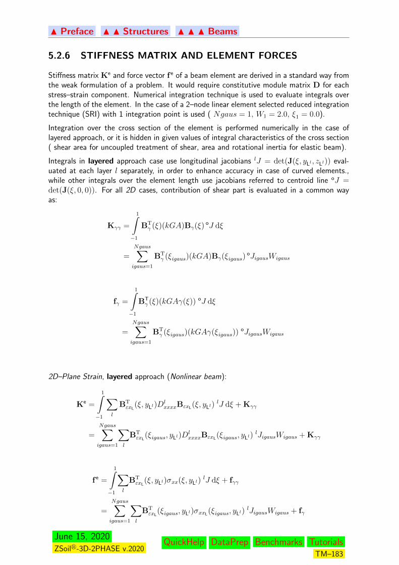
N Preface N N Structures N N N Beams
5.2.6 STIFFNESS MATRIX AND ELEMENT FORCES
Stiffness matrix Ke and force vector f e of a beam element are derived in a standard way fromthe weak formulation of a problem. It would require constitutive module matrix D for eachstress–strain component. Numerical integration technique is used to evaluate integrals overthe length of the element. In the case of a 2–node linear element selected reduced integrationtechnique (SRI) with 1 integration point is used ( Ngaus = 1, W1 = 2.0, ξ1 = 0.0).
Integration over the cross section of the element is performed numerically in the case oflayered approach, or it is hidden in given values of integral characteristics of the cross section( shear area for uncoupled treatment of shear, area and rotational inertia for elastic beam).
Integrals in layered approach case use longitudinal jacobians lJ = det(J(ξ, yLl , zLl)) eval-uated at each layer l separately, in order to enhance accuracy in case of curved elements.,while other integrals over the element length use jacobians referred to centroid line oJ =det(J(ξ, 0, 0)). For all 2D cases, contribution of shear part is evaluated in a common wayas:
Kγγ =
1∫−1
BTγ (ξ)(kGA)Bγ(ξ)
oJ dξ
=
Ngaus∑igaus=1
BTγ (ξigaus)(kGA)Bγ(ξigaus)
oJigausWigaus
fγ =
1∫−1
BTγ (ξ)(kGAγ(ξ)) oJ dξ
=
Ngaus∑igaus=1
BTγ (ξigaus)(kGAγ(ξigaus))
oJigausWigaus
2D–Plane Strain, layered approach (Nonlinear beam):
Ke =
1∫−1
∑l
BTεxL
(ξ, yLl)DlxxxxBεxL
(ξ, yLl) lJ dξ + Kγγ
=
Ngaus∑igaus=1
∑l
BTεxL
(ξigaus, yLl)DlxxxxBεxL
(ξigaus, yLl) lJigausWigaus + Kγγ
f e =
1∫−1
∑l
BTεxL
(ξ, yLl)σxx(ξ, yLl) lJ dξ + fγγ
=
Ngaus∑igaus=1
∑l
BTεxL
(ξigaus, yLl)σxxL(ξigaus, yLl) lJigausWigaus + fγ
June 15, 2020ZSoilr-3D-2PHASE v.2020
QuickHelp DataPrep Benchmarks TutorialsTM–183
N Preface N N Structures N N N Beams
Plane Strain , integral approach (Elastic beam model):
Ke =
1∫−1
[BTε (ξ); BT
κ (ξ)] [ EA 0
0 ELz
] [Bε(ξ)Bκ(ξ)
]oJ dξ + Kγγ
=
Ngaus∑igaus=1
[BTε (ξigaus); BT
κ (ξigaus)] [ EA 0
0 ELz
] [Bε(ξigaus)Bκ(ξigaus)
]oJigausWigaus + Kγγ
f e =
1∫−1
[BTε (ξ); BT
κ (ξ)] [ EAε(ξ)
EIzκ(ξ)
]oJ dξ + fγ =
Ngaus∑igaus=1
[BTε (ξigaus); BT
κ (ξigaus)] [ EAε(ξigaus)
EIzκ(ξigaus)
]oJigausWigaus + fγ
2D–Axisymmetry, layered approach (Nonlinear beam):
Ke = 2π
1∫−1
∑l
[BTεxL
(ξ, yLl); BTεzL
(ξ, yLl)] [
Dl] [ BεxL
(ξ, yLl)BεzL
(ξ, yLl)
]r(ξ) lJdξ + rKγγ
= 2π
(Ngaus∑igaus=1
∑l
[BTεxL
(ξigaus, yLl); BTεzL
(ξigaus, yLl)] [
Dl] [ BεxL
(ξigaus, yLl)BεzL
(ξigaus, yLl)
])r(ξigaus)
lJigausWigaus + 2πrKγγ
f e = 2π
1∫−1
∑l
[BTεxL
(ξ, yLl); BTεzL
(ξ, yLl)] [ σxx(ξ, yLl)
σxz(ξ, yLl)
]r(ξ) lJ dξ + rfγ
=
2π
(Ngaus∑igaus=1
∑l
[BTεxL
(ξigaus, yLl); BTεzL
(ξigaus, yLl)] [ σxx(ξigaus, yLl)
σxz(ξigaus, yLl)
])r(ξigaus)
lJigausWigaus + 2πrfγ
where constitutive module matrix: Dl(2×2) =
[Dxxxx Dxxzz
Dzzxx Dzzzz
].
3D analysis:
For both layered and integral approaches, treatment of transversal shear and torsion is de–coupled from treatment of bending and extension states. Thus element stiffness and forcesare split according to:
Ke = KeN−M +
∑i=x,y
Keγi + Ke
Ψ
June 15, 2020ZSoilr-3D-2PHASE v.2020
QuickHelp DataPrep Benchmarks TutorialsTM–184
N Preface N N Structures N N N Beams
f e = f eN−M +
∑i=x,y
f eγi + f e
Ψ
The contributions common for layered and integral approaches are:
shear :
Keγi =
1∫−1
BTγxi
(ξ)kiGABγxi(ξ)oJ dξ
=
Ngaus∑igaus=1
BTγxi
(ξigaus)kiGABγxi(ξigaus)oJigausWigaus
f eγi =
1∫−1
BTγxi
(ξ)kiGAγxi(ξ)oJ dξ
=
Ngaus∑igaus=1
BTγxi
(ξigaus)kiGAγxi(ξigaus)oJigausWigaus
torsion:
KeΨ =
1∫−1
BTΨ(ξ)GIxBΨ(ξ) oJ dξ
=
Ngaus∑igaus=1
BTΨ(ξigaus)GIxBΨ(ξigaus)
oJigausWigaus
f eΨ =
1∫−1
BTΨ(ξ)GIxΨ(ξ) oJ dξ
=
Ngaus∑igaus=1
BTΨ(ξigaus)GIxΨ(ξigaus)
oJigausWigaus
Bending and extension states are treated in different ways:
layered approach (Nonlinear beam model):
KeN−M =
1∫−1
∑l
BTεxL
(ξ, yLl , zLl)DlxxxxBεxL
(ξ, yLl , zLl) lJ dξ
=
Ngaus∑igaus=1
∑l
BTεxL
(ξigaus, yLl , zLl)DlxxxxBεxL
(ξigaus, yLl , zLl) lJigausWigaus
June 15, 2020ZSoilr-3D-2PHASE v.2020
QuickHelp DataPrep Benchmarks TutorialsTM–185
N Preface N N Structures N N N Beams
f eN−M =
1∫−1
∑l
BTεxL
(ξ, yLl , zLl)σxx(ξ, yLl , zLl) lJ dξ
=
Ngaus∑igaus=1
∑l
BTεxL
(ξigaus, yLl , zLl)σxx(ξigaus, yLl , zLl) lJigausWigaus
integral approach (Elastic beam model):
KeN−M =
1∫−1
[BTε (ξ); BT
κy(ξ); BTκz(ξ)
] EA 0 00 EIy 00 0 EIz
Bε(ξ)Bκy(ξ)Bκz(ξ)
oJ dξ
=
Ngaus∑igaus=1
[BTε (ξigaus); BT
κy(ξigaus); BTκz(ξigaus)
] EA 0 00 EIy 00 0 EIz
Bε(ξigaus)
Bκy(ξigaus)Bκz(ξigaus)
oJigausWigaus
f eN−M =
1∫−1
[BTε (ξ) BT
κy(ξ) BTκz(ξ)
] EAε(ξ)EIyκy(ξ)EIzκz(ξ)
oJ dξ
=
Ngaus∑igaus=1
[BTε (ξigaus); BT
κy(ξigaus); BTκz(ξigaus)
] EAε(ξigaus)EIyκy(ξigaus)EIzκz(ξigaus)
oJigausWigaus
The element load p is assumed to act along the centroid line leading to load induced forcesevaluated as:
fp =
1∫−1
NT(ξ)p oJ dξ =
Ngaus∑igaus=1
NT(ξigaus)poJigausWigaus
N(ξ) =[Ni(ξ)I(dim)
], i = 1, Nen
All element forces and stiffness, as given above, are referred to centroidal nodes of theelement. Prior to the agregation to global ones, they are submitted to Master–centroid(offset) transformation, see Appendix 5.6.1 .
June 15, 2020ZSoilr-3D-2PHASE v.2020
QuickHelp DataPrep Benchmarks TutorialsTM–186

N Preface N N Structures N N N Beams
5.2.7 MASTER-CENTROID (OFFSET) TRANSFORMATION
In order to deal with the frequently encountered situation where beam elements are connectedto other elements of the model by nodes, which are not the centroids of a beam cross section,offset transformation of element displacement, forces and stiffness is introduced. The DOFof the element are placed on its ”master” nodes defining connectivity. Based on rigid bodymovement of the ”master”, translation and rotation displacements of the ”centroid” areevaluated.
For the details of ”master-slave” offset transformation see the Appendix 5.6.1 .
June 15, 2020ZSoilr-3D-2PHASE v.2020
QuickHelp DataPrep Benchmarks TutorialsTM–187

N Preface N N Structures N N N Beams
5.2.8 RELAXATION OF INTERNAL DOF
Stiffness matrix and force vector derived above concerns element with all DOF active. Situa-tion when user demanded group of DOF is relaxed (what means that no forces are transmittedby the element in selected directions).The directions of relaxed DOF might be related to localelement directions at both ends of the element.
If given directions at beam node are relaxed, the node is implicitly duplicated and DSC(Node-to-node interface ) elements are introduced to the model. The stiffness of that in-terface remains 0 at relaxed direction, while it is assumed to take penalty values, estimatedautomaticaly from beam stiffness on fixed DOF.
June 15, 2020ZSoilr-3D-2PHASE v.2020
QuickHelp DataPrep Benchmarks TutorialsTM–188
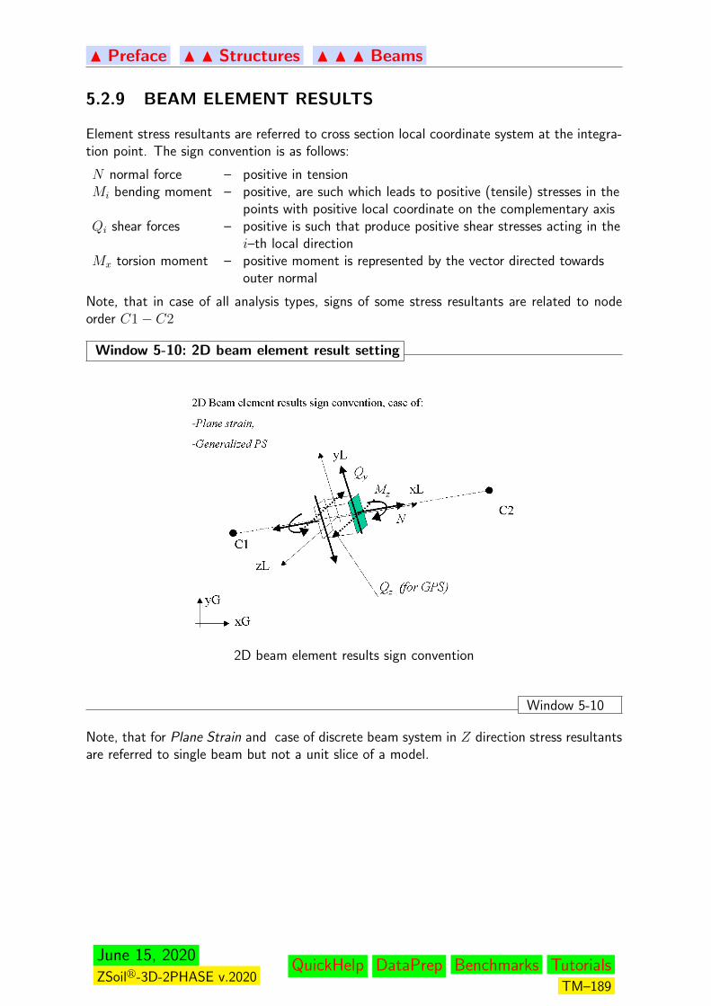
N Preface N N Structures N N N Beams
5.2.9 BEAM ELEMENT RESULTS
Element stress resultants are referred to cross section local coordinate system at the integra-tion point. The sign convention is as follows:
N normal force – positive in tensionMi bending moment – positive, are such which leads to positive (tensile) stresses in the
points with positive local coordinate on the complementary axisQi shear forces – positive is such that produce positive shear stresses acting in the
i–th local directionMx torsion moment – positive moment is represented by the vector directed towards
outer normal
Note, that in case of all analysis types, signs of some stress resultants are related to nodeorder C1− C2
Window 5-10: 2D beam element result setting
2D beam element results sign convention
Window 5-10
Note, that for Plane Strain and case of discrete beam system in Z direction stress resultantsare referred to single beam but not a unit slice of a model.
June 15, 2020ZSoilr-3D-2PHASE v.2020
QuickHelp DataPrep Benchmarks TutorialsTM–189

N Preface N N Structures N N N Beams
Window 5-11: Axisymetric shell element result setting
Axisymmetric shell element results sign convention
Window 5-11
Note, that in the case of Axisymmetry, evaluated stress resultants are referred to the unitlength of the axi–symmetric shell both in circumference and meridian direction.
Window 5-12: 3D beam element result setting
3D beam element results sign convention
Window 5-12
June 15, 2020ZSoilr-3D-2PHASE v.2020
QuickHelp DataPrep Benchmarks TutorialsTM–190

N Preface N N Structures
5.3 SHELLS
Following paragraphs present most important aspects of applied shell elements
BASIC ASSUMPTIONS OF SHELL ANALYSIS
SETTING OF THE ELEMENT GEOMETRY
ELEMENT MAPPING AND COORDINATE SYSTEMS
CROSS–SECTION MODELS
DISPLACEMENT AND STRAIN FIELD WITHIN THE ELEMENT
TREATMENT OF TRANSVERSAL SHEAR
WEAK FORMULATION OF EQUILIBRIUM
STIFFNESS MATRIX AND ELEMENT FORCES
LOADS
SHELL ELEMENT RESULTS
June 15, 2020ZSoilr-3D-2PHASE v.2020
QuickHelp DataPrep Benchmarks TutorialsTM–191
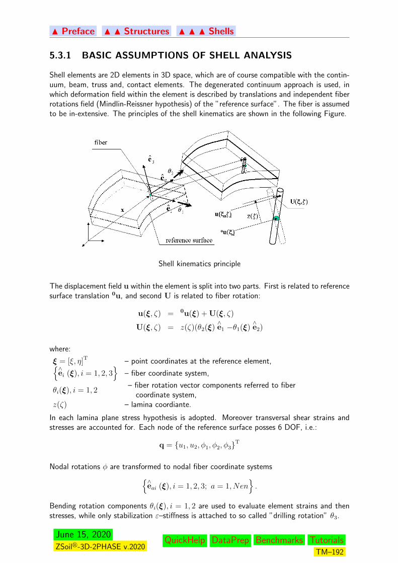
N Preface N N Structures N N N Shells
5.3.1 BASIC ASSUMPTIONS OF SHELL ANALYSIS
Shell elements are 2D elements in 3D space, which are of course compatible with the contin-uum, beam, truss and, contact elements. The degenerated continuum approach is used, inwhich deformation field within the element is described by translations and independent fiberrotations field (Mindlin-Reissner hypothesis) of the ”reference surface”. The fiber is assumedto be in-extensive. The principles of the shell kinematics are shown in the following Figure.
Shell kinematics principle
The displacement field u within the element is split into two parts. First is related to referencesurface translation 0u, and second U is related to fiber rotation:
u(ξ, ζ) = 0u(ξ) + U(ξ, ζ)
U(ξ, ζ) = z(ζ)(θ2(ξ)∧e1 −θ1(ξ)
∧e2)
where:
ξ = [ξ, η]T – point coordinates at the reference element,∧ei (ξ), i = 1, 2, 3
– fiber coordinate system,
θi(ξ), i = 1, 2– fiber rotation vector components referred to fiber
coordinate system,z(ζ) – lamina coordiante.
In each lamina plane stress hypothesis is adopted. Moreover transversal shear strains andstresses are accounted for. Each node of the reference surface posses 6 DOF, i.e.:
q = u1, u2, φ1, φ2, φ3T
Nodal rotations φ are transformed to nodal fiber coordinate systems∧eai (ξ), i = 1, 2, 3; a = 1, Nen
.
Bending rotation components θi(ξ), i = 1, 2 are used to evaluate element strains and thenstresses, while only stabilization ε–stiffness is attached to so called ”drilling rotation” θ3.
June 15, 2020ZSoilr-3D-2PHASE v.2020
QuickHelp DataPrep Benchmarks TutorialsTM–192
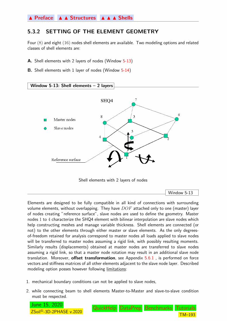
N Preface N N Structures N N N Shells
5.3.2 SETTING OF THE ELEMENT GEOMETRY
Four (8) and eight (16) nodes shell elements are available. Two modeling options and relatedclasses of shell elements are:
A. Shell elements with 2 layers of nodes (Window 5-13)
B. Shell elements with 1 layer of nodes (Window 5-14)
Window 5-13: Shell elements – 2 layers
Shell elements with 2 layers of nodes
Window 5-13
Elements are designed to be fully compatible in all kind of connections with surroundingvolume elements, without overlapping. They have DOF attached only to one (master) layerof nodes creating ”reference surface”, slave nodes are used to define the geometry. Masternodes 1 to 4 characterize the SHQ4 element with bilinear interpolation are slave nodes whichhelp constructing meshes and manage variable thickness. Shell elements are connected (ornot) to the other elements through either master or slave elements. As the only degrees-of-freedom retained for analysis correspond to master nodes all loads applied to slave nodeswill be transferred to master nodes assuming a rigid link, with possibly resulting moments.Similarly results (displacements) obtained at master nodes are transferred to slave nodesassuming a rigid link, so that a master node rotation may result in an additional slave nodetranslation. Moreover, offset transformation, see Appendix 5.6.1 , is performed on forcevectors and stiffness matrices of all other elements adjacent to the slave node layer. Describedmodeling option posses however following limitations:
1. mechanical boundary conditions can not be applied to slave nodes,
2. while connecting beam to shell elements Master-to-Master and slave-to-slave conditionmust be respected.
June 15, 2020ZSoilr-3D-2PHASE v.2020
QuickHelp DataPrep Benchmarks TutorialsTM–193
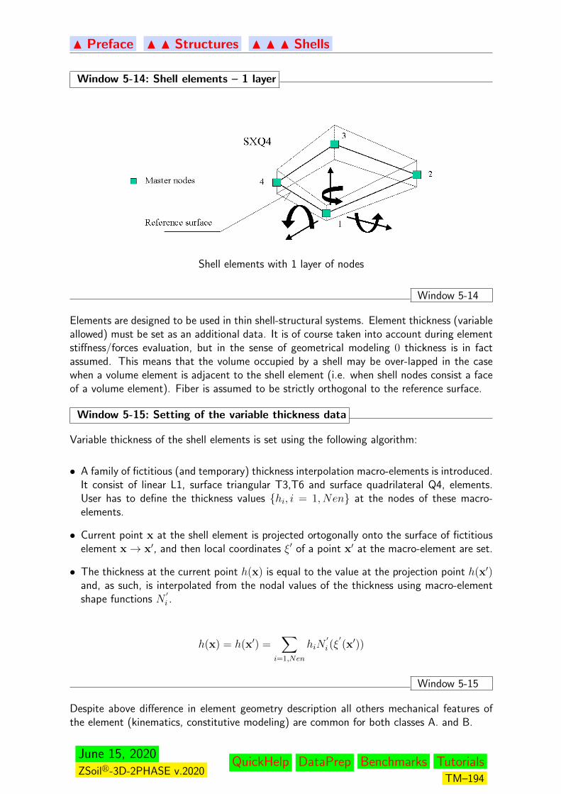
N Preface N N Structures N N N Shells
Window 5-14: Shell elements – 1 layer
Shell elements with 1 layer of nodes
Window 5-14
Elements are designed to be used in thin shell-structural systems. Element thickness (variableallowed) must be set as an additional data. It is of course taken into account during elementstiffness/forces evaluation, but in the sense of geometrical modeling 0 thickness is in factassumed. This means that the volume occupied by a shell may be over-lapped in the casewhen a volume element is adjacent to the shell element (i.e. when shell nodes consist a faceof a volume element). Fiber is assumed to be strictly orthogonal to the reference surface.
Window 5-15: Setting of the variable thickness data
Variable thickness of the shell elements is set using the following algorithm:
• A family of fictitious (and temporary) thickness interpolation macro-elements is introduced.It consist of linear L1, surface triangular T3,T6 and surface quadrilateral Q4, elements.User has to define the thickness values hi, i = 1, Nen at the nodes of these macro-elements.
• Current point x at the shell element is projected ortogonally onto the surface of fictitiouselement x→ x′, and then local coordinates ξ′ of a point x′ at the macro-element are set.
• The thickness at the current point h(x) is equal to the value at the projection point h(x′)and, as such, is interpolated from the nodal values of the thickness using macro-elementshape functions N
′i .
h(x) = h(x′) =∑
i=1,Nen
hiN′
i (ξ′(x′))
Window 5-15
Despite above difference in element geometry description all others mechanical features ofthe element (kinematics, constitutive modeling) are common for both classes A. and B.
June 15, 2020ZSoilr-3D-2PHASE v.2020
QuickHelp DataPrep Benchmarks TutorialsTM–194
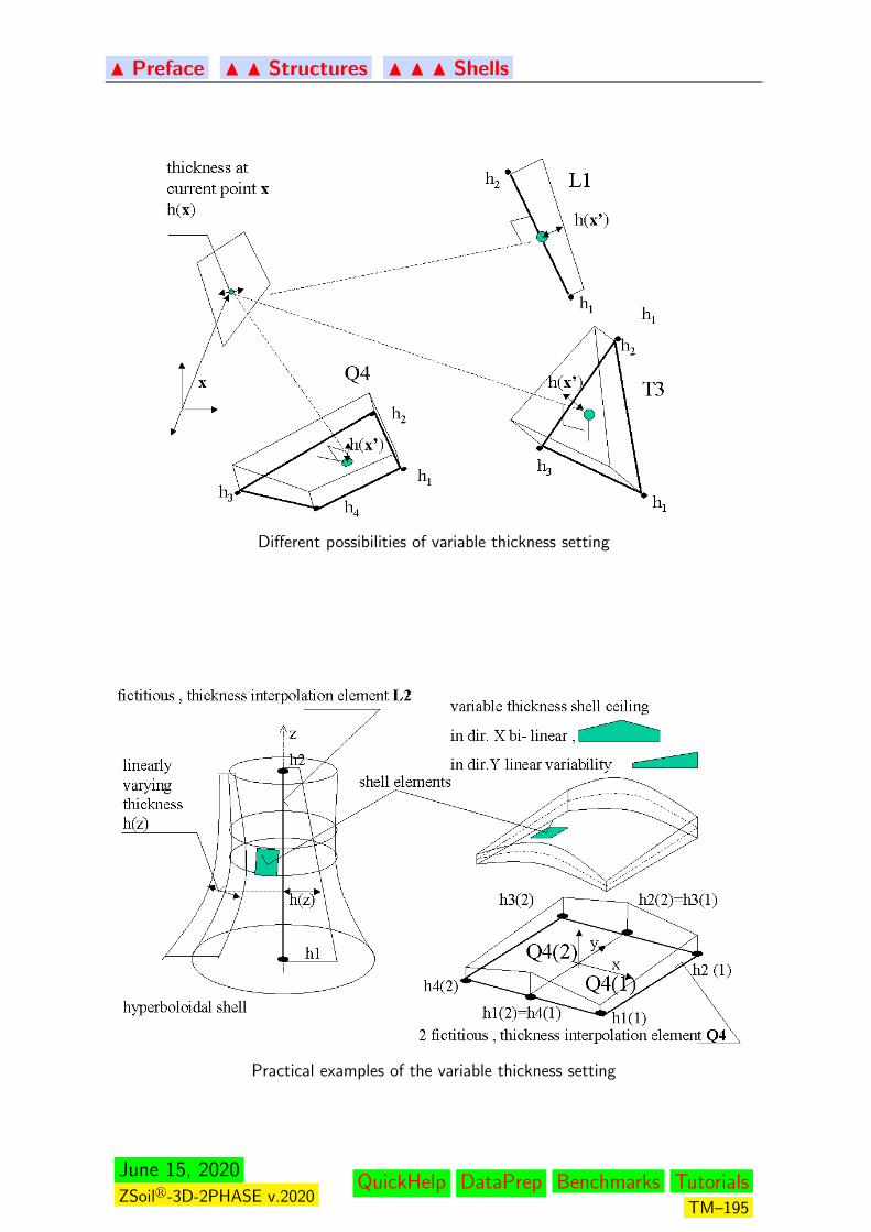
N Preface N N Structures N N N Shells
Different possibilities of variable thickness setting
Practical examples of the variable thickness setting
June 15, 2020ZSoilr-3D-2PHASE v.2020
QuickHelp DataPrep Benchmarks TutorialsTM–195

N Preface N N Structures N N N Shells
5.3.3 ELEMENT MAPPING AND COORDINATE SYSTEMS
Given construction of the shell element is common for each type of shell element SXQ4,SHQ4.
Window 5-16: Shell elements coordinate systems and mapping
• Nodal basis, after 1
for each node a = 1, Nen
eai, i = 1, 2, 3 =
[ea1, ea2, ea3] =
nz +
1
1 + nzn2y − 1
1 + nznxny nx
− 1
1 + nznxny nz +
1
1 + nzn2x ny
−nx −ny nz
, ifnz 6= −1
1 0 0
0 −1 0
0 0 −1
, ifnz = −1
where: na = [nx, ny, nz]T is element reference surface normal at node a.
• Mapping from the reference element is constructed as follows, after2: x(ξ, η, ζ) = ox(ξ, η)+X(ξ, η, ζ)with:
reference surface:ox(ξ, η) =
∑a=1,Nen
Na(ξ, η) oxa;
position on the director:
X(ξ, η, ζ) =∑
a=1,Nen
Na(ξ, η) za(ζ)ea3;
where:
za(ζ) =1
2(1 + ζ)z+
a +1
2(1− ζ)z−a
1J.L. Batoz, G. Dhatt, Modelisation des structures par element finis, Ed.Hermes, Paris 1992.2T.J.R. Hughes, The Finite Element method, Ed.Prentice–Hall Inc.1988.
June 15, 2020ZSoilr-3D-2PHASE v.2020
QuickHelp DataPrep Benchmarks TutorialsTM–196
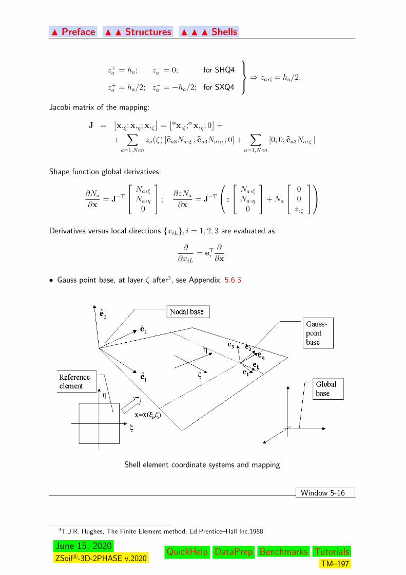
N Preface N N Structures N N N Shells
z+a = ha; z−a = 0; for SHQ4
z+a = ha/2; z−a = −ha/2; for SXQ4
⇒ za,ζ = ha/2.
Jacobi matrix of the mapping:
J =[x,ξ; x,η; x,ζ
]=[ox,ξ;
o x,η; 0]
+
+∑
a=1,Nen
za(ζ) [ea3Na,ξ ; ea3Na,η ; 0] +∑
a=1,Nen
[0; 0; ea3Na,ζ ]
Shape function global derivatives:
∂Na
∂x= J−T
Na,ξNa,η
0
;∂zNa
∂x= J−T
z Na,ξNa,η
0
+Na
00z,ζ
Derivatives versus local directions xiL, i = 1, 2, 3 are evaluated as:
∂
∂xiL= eT
i
∂
∂x.
• Gauss point base, at layer ζ after3, see Appendix: 5.6.3
Shell element coordinate systems and mapping
Window 5-16
3T.J.R. Hughes, The Finite Element method, Ed.Prentice–Hall Inc.1988.
June 15, 2020ZSoilr-3D-2PHASE v.2020
QuickHelp DataPrep Benchmarks TutorialsTM–197

N Preface N N Structures N N N Shells
5.3.4 CROSS–SECTION MODELS
Independently from the element geometry description, two approaches to modeling of thecross sectional behavior of a shell are available. They are:
(i) homogeneous section, elastic model.
The cross section is fully described by elastic material data, i.e. Young module E and Poissonratio ν.Note, that element thickness is set as geometric data, independent from cross sectionmodel. Numerical integration along the depth of an element is performed using 2-point Gaussrule.
(ii) layered model (non–homogenous section or/and material non–linearity).
The cross section is understood as a set of layers with possible different material models ineach. In the case of homogenous section but non-linear material model introduction of layersmay be understood as the specification of integration rule, different than 2-point Gauss ruleused in the case of homogenous elastic section.
The following data must be specified for the whole section:
– number of layers Nlayer ≤ NLAY ER MAX = 20
– elastic properties E, ν
– averaged volume unit weight ( for evaluation of gravity load )
while for each layer required are:
– zi, the position of the layer center (relative or the distance from top/bottom)
– wi = hih
, the relative depth of the layer or, for the fiber model, the area of fiber
per unit length.
– indication of a material model attached to the layer.
The models to be used in that context are : elastic , elasto-plastic Menetrey–
Willam, 1D elasto-plastic fiber model, In the latter case, for each elasto–
plastic fiber model
– E, the elastic modulus,
– fty, the tensile yield stress,
– fcy, the compressive yield stress,
– nx, ny, nz direction cosines of a unit vector; the projection of n on the element
surface will define the fiber orientation, see Appendix 5.6.2 and example in the followingfigure.
June 15, 2020ZSoilr-3D-2PHASE v.2020
QuickHelp DataPrep Benchmarks TutorialsTM–198
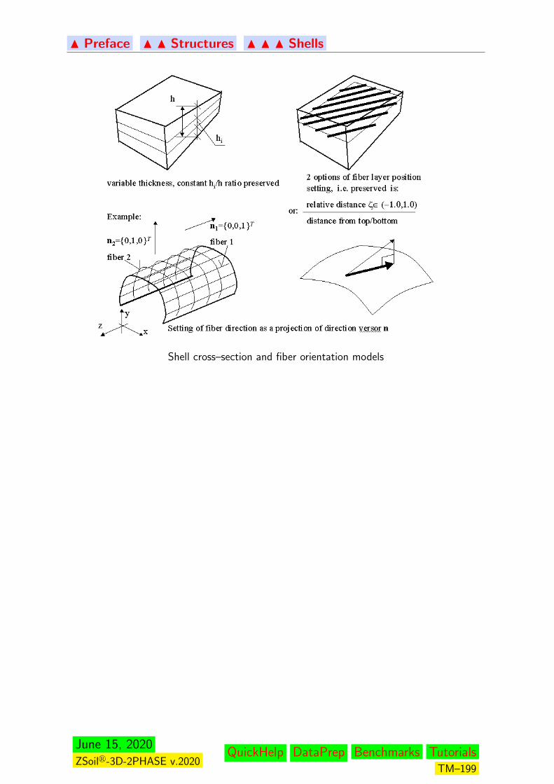
N Preface N N Structures N N N Shells
Shell cross–section and fiber orientation models
June 15, 2020ZSoilr-3D-2PHASE v.2020
QuickHelp DataPrep Benchmarks TutorialsTM–199

N Preface N N Structures N N N Shells
5.3.5 DISPLACEMENT AND STRAIN FIELD WITHIN THE ELE-MENT
Assumed kinematic hypothesis together with interpolating (shape) functions built upon ref-erence element with node number Nen = 4 (SHQ4, SXQ4) lead to the following expressionsfor the displacement field within the element. The displacement field may be expressed :
• in terms of nodal translations ua and rotations θa1, θa2 in the directions of nodal basevectors e1, e2 tangent to the element reference surface, as:
u(ξ, ζ) =∑
a=1,Nen
Na(ξ)ua +∑
a=1,Nen
Na(ξ)z(ζ)(ea1θa2 − ea2θa1)
Above will be used to evaluate element strains.
• in terms of element DOF vector q, including global components of rotations φ usinggeneralized shape function matrix N, as:
u(ξ, ζ) = N(ξ, ζ)q
q = [ua1, ua2, ua3, φa1, φa2, φa3]T , a = 1, Nen
N(ξ, ζ) =[Na(ξ)I3×3; z(ζ)Na(ξ)(ea1e
Ta2 − ea2e
Ta1)], a = 1, Nen
Above, will be used for evaluation of element equivalent forces, and for numerical realizationof anchoring, see p. 5.1.3.1 Strain approximation is built upon nodal translations uaand rotations θa1, θa2 in the directions of nodal base vectors e1, e2 tangent to the elementreference surface, consisting 5 components of DOF vector q(5)
q(5) = [ua1, ua2, ua3, θa1, θa2]T , a = 1, Nen
εm =
[∂u1L
∂x1L
,∂u2L
∂x2L
,∂u1L
∂x2L
+∂u2L
∂x1L
]= Bmq(5)
εs =
[∂u1L
∂x3L
+∂u3L
∂x1L
,∂u2L
∂x3L
+∂u3L
∂x2L
]= Bsq(5)
Membrane strains are evaluated in unified way for all options considered, with Bm matrixtaking form:
... u... θα, α = 1, 2
...
Bm =
eT1
∂Na
∂x1L
ωa1α∂zNa
∂x1L
eT1
∂Na
∂x1L
... ωa2α∂zNa
∂x2L
eT1
∂Na
∂x2L
+ eT2
∂Na
∂x1L
ωa1α∂zNa
∂x2L
+ ωa2α∂zNa
∂x1L
, a = 1, Nen
June 15, 2020ZSoilr-3D-2PHASE v.2020
QuickHelp DataPrep Benchmarks TutorialsTM–200
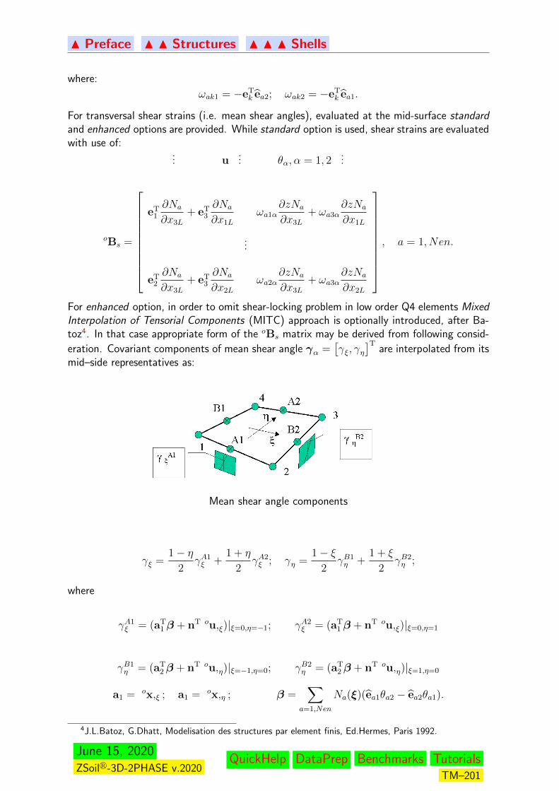
N Preface N N Structures N N N Shells
where:
ωak1 = −eTk ea2; ωak2 = −eT
k ea1.
For transversal shear strains (i.e. mean shear angles), evaluated at the mid-surface standardand enhanced options are provided. While standard option is used, shear strains are evaluatedwith use of:
... u... θα, α = 1, 2
...
oBs =
eT1
∂Na
∂x3L
+ eT3
∂Na
∂x1L
ωa1α∂zNa
∂x3L
+ ωa3α∂zNa
∂x1L
...
eT2
∂Na
∂x3L
+ eT3
∂Na
∂x2L
ωa2α∂zNa
∂x3L
+ ωa3α∂zNa
∂x2L
, a = 1, Nen.
For enhanced option, in order to omit shear-locking problem in low order Q4 elements MixedInterpolation of Tensorial Components (MITC) approach is optionally introduced, after Ba-toz4. In that case appropriate form of the oBs matrix may be derived from following consid-
eration. Covariant components of mean shear angle γα =[γξ, γη
]Tare interpolated from its
mid–side representatives as:
Mean shear angle components
γξ =1− η
2γA1ξ +
1 + η
2γA2ξ ; γη =
1− ξ2
γB1η +
1 + ξ
2γB2η ;
where
γA1ξ = (aT
1 β + nT ou,ξ)|ξ=0,η=−1; γA2ξ = (aT
1 β + nT ou,ξ)|ξ=0,η=1
γB1η = (aT
2 β + nT ou,η)|ξ=−1,η=0; γB2η = (aT
2 β + nT ou,η)|ξ=1,η=0
a1 = ox,ξ ; a1 = ox,η ; β =∑
a=1,Nen
Na(ξ)(ea1θa2 − ea2θa1).
4J.L.Batoz, G.Dhatt, Modelisation des structures par element finis, Ed.Hermes, Paris 1992.
June 15, 2020ZSoilr-3D-2PHASE v.2020
QuickHelp DataPrep Benchmarks TutorialsTM–201

N Preface N N Structures N N N Shells
After transformation components of mean shear angle εS = [γ1L, γ2L]T in local Gauss pointbase Q are obtained as:
εS = CTγα; with: C =
aT1 a1 aT
1 a2
symm aT2 a2
−1 aT
1 e1 aT1 e2
aT1 e2 aT
2 e2
.
June 15, 2020ZSoilr-3D-2PHASE v.2020
QuickHelp DataPrep Benchmarks TutorialsTM–202
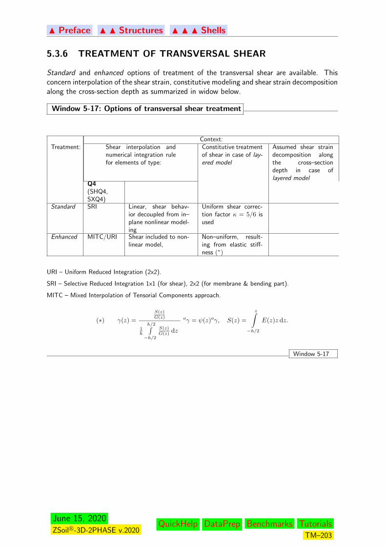
N Preface N N Structures N N N Shells
5.3.6 TREATMENT OF TRANSVERSAL SHEAR
Standard and enhanced options of treatment of the transversal shear are available. Thisconcern interpolation of the shear strain, constitutive modeling and shear strain decompositionalong the cross-section depth as summarized in widow below.
Window 5-17: Options of transversal shear treatment
Context:Treatment: Shear interpolation and
numerical integration rulefor elements of type:
Constitutive treatmentof shear in case of lay-ered model
Assumed shear straindecomposition alongthe cross–sectiondepth in case oflayered model
Q4(SHQ4,SXQ4)
Standard SRI Linear, shear behav-ior decoupled from in–plane nonlinear model-ing
Uniform shear correc-tion factor κ = 5/6 isused
Enhanced MITC/URI Shear included to non-linear model,
Non–uniform, result-ing from elastic stiff-ness (∗)
URI – Uniform Reduced Integration (2x2).
SRI – Selective Reduced Integration 1x1 (for shear), 2x2 (for membrane & bending part).
MITC – Mixed Interpolation of Tensorial Components approach.
(∗) γ(z) =
S(z)G(z)
1h
h/2∫−h/2
S(z)G(z) dz
oγ = ψ(z)oγ, S(z) =
z∫−h/2
E(z)z dz.
Window 5-17
June 15, 2020ZSoilr-3D-2PHASE v.2020
QuickHelp DataPrep Benchmarks TutorialsTM–203
N Preface N N Structures N N N Shells
5.3.7 WEAK FORMULATION OF EQUILIBRIUM
Formulation of the equilibrium equations are derived from virtual work principle (VWP), which in takesgeneral form:
find σ such that:
for any δε, δu ∫V
δεTσ dV −∫V
δuTb dV = 0
In each detailed case, the particular form of VWP is as follows, using the notation:
εm =[εxxL εyyL γxyL
]T– membrane strains
σm =[σxxL σyyL σxyL
]T– membrane stresses
εs =[γxzL γyzL
]T– shear strains
σs =[σxzL σyzL
]T– shear stresses
ε = [εm, εs]T – full strains and stresses
V – volume of the elementΩ – reference surface areab – body forces
Delss =
[G 00 G
]– shear part of linear constituive matrix
with
κ – shear correction factor (=5/6 for homogeneous section)G – Kirchhoff modulih – element thickness.
• homogenous section, elastic modelfind σ such that:for any δε, δγ, δu ∫
V
δεTmσm dV +
∫Ω
δγTs κhD
elssγs dΩ−
∫V
δuTbdV = 0
• layered section, possible nonlinear model, standard treatment of shear (shear de-coupled from membranepart in constitutive model)
find σ such that:for any δε, δγ, δu∫
Ω
∑i
(δεlm)Tσlm∆hl dΩ +
∫Ω
δγTs κhD
elssγs dΩ−
∫V
δuTb dV = 0
• layered section, possible nonlinear model, enhanced treatment of shear (shear included in constitutivemodel)
find σ such that:for any δε, δγ, δu ∫
Ω
∑i
(δεlm)Tσlm∆hl dΩ−∫V
δuTbdV = 0
Moreover, in the case of enhanced shear treatment for SHQ4,SXQ4 elements MITC ( Mixed Interpolation ofTensorial Components ) approach is applied.
June 15, 2020ZSoilr-3D-2PHASE v.2020
QuickHelp DataPrep Benchmarks TutorialsTM–204

N Preface N N Structures N N N Shells
5.3.8 STIFFNESS MATRIX AND ELEMENT FORCES
The formulas for element stiffness matrix K(5×5) and force vectors concern 5DOF component vectorsq(5), f(5) with rotations /moments related to nodal tangent directions.
• layered model with standard treatment of shear or homogenous section , elastic model:
K(5×5) =
∫Ω
Nlayer∑ilayer=1
BTmDmmBmjhilayer dξ dη +
∫Ω
oBTs κhD
elss
oBsj dξ dη
f(5) =
∫Ω
Nlayer∑ilayer=1
BTmσmjhilayer dξ dη +
∫Ω
oBTs κhD
elss
oεsj dξ dη
where o() concerns mean shear strains.
• layered model with enhanced treatment of shear:
K(5×5) =
∫Ω
Nlayer∑ilayer=1
[BTm,B
Ts
] [ Dmm Dms
Dsm Dss
] [Bm
Bs
]jhilayer dξ dη
f(5) =
∫Ω
Nlayer∑ilayer=1
[BTm,B
Ts
] [ σmσs
]jhilayer dξ dη
Bs = ψ(zilayer)oBs
In all above integrals Gauss type integration is performed over the surface of the element as specified inWindow 5-17. Integration in the direction of element depth is based on user defined layer setting (layeredmodel) or on 2 point Gauss rule in case of homogenous section, elastic model.
5 − DOF vectors and matrix are put into full 6 − DOF ones and stabilizing terms are added to stiffnessmatrix on the positions of 6th DOF (drilling rotations), in order to avoid singularity in case of co-planarityof elements adjacent to a node.
K =
[Kab(5×5) 00 kdrill
ab
], a, b = 1, Nen
f =[fa(5), 0 , a = 1, Nen
]kdrillab = α
∫Ω
NaNbGhdΩ, α ∼= 10−6
Subsequently, rotational part is transformed to global coordinate system :
fG = Tf
KG = TKTT
where
T =
T1 s 0 s 0...
. . ....
0 Ta 0...
. . ....
0 s 0 s TNen
,
Ta =
[I3×3 00 [ea1, ea2, ea3]
], a = 1, Nen.
June 15, 2020ZSoilr-3D-2PHASE v.2020
QuickHelp DataPrep Benchmarks TutorialsTM–205

N Preface N N Structures N N N Shells
5.3.9 LOADS
Gravity, nodal and surface loads can be applied. Gravity corresponds to body forces. In a case of shell 2node layer elements (option A) nodal forces can be applied to either master or slave nodes. Also surfaceloads are specified on fictitious surface elements S Q4 which may be set on slave or master layer of nodes.Equivalent nodal force vector consist of forces as well as moments, evaluated with use of generalized shapefunction matrix N as:
fp =
∫V e
NTpdV
Thermal loads can also be accounted for; thermal analysis is always performed on a continuum element andthen ε thermal is projected into shell material data at each layer.
June 15, 2020ZSoilr-3D-2PHASE v.2020
QuickHelp DataPrep Benchmarks TutorialsTM–206
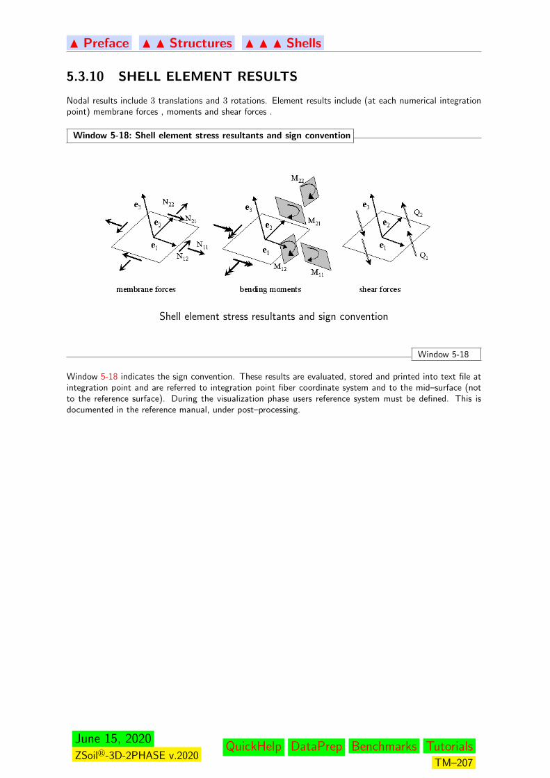
N Preface N N Structures N N N Shells
5.3.10 SHELL ELEMENT RESULTS
Nodal results include 3 translations and 3 rotations. Element results include (at each numerical integrationpoint) membrane forces , moments and shear forces .
Window 5-18: Shell element stress resultants and sign convention
Shell element stress resultants and sign convention
Window 5-18
Window 5-18 indicates the sign convention. These results are evaluated, stored and printed into text file atintegration point and are referred to integration point fiber coordinate system and to the mid–surface (notto the reference surface). During the visualization phase users reference system must be defined. This isdocumented in the reference manual, under post–processing.
June 15, 2020ZSoilr-3D-2PHASE v.2020
QuickHelp DataPrep Benchmarks TutorialsTM–207
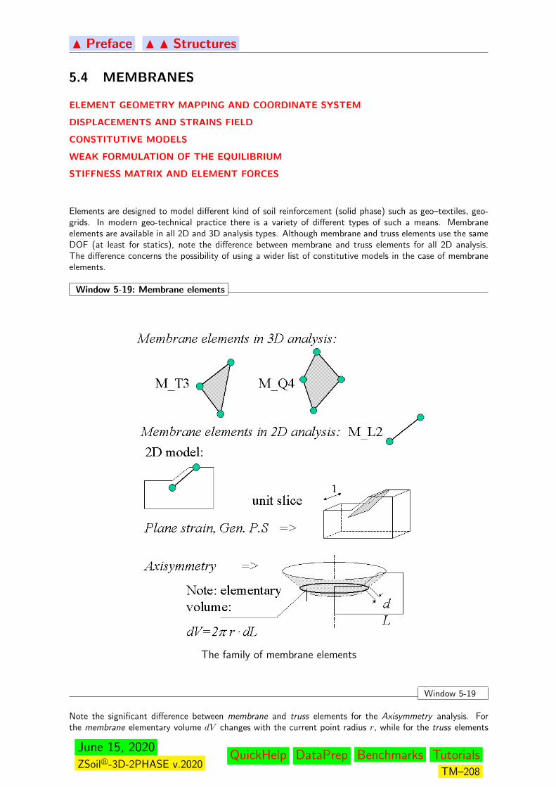
N Preface N N Structures
5.4 MEMBRANES
ELEMENT GEOMETRY MAPPING AND COORDINATE SYSTEM
DISPLACEMENTS AND STRAINS FIELD
CONSTITUTIVE MODELS
WEAK FORMULATION OF THE EQUILIBRIUM
STIFFNESS MATRIX AND ELEMENT FORCES
Elements are designed to model different kind of soil reinforcement (solid phase) such as geo–textiles, geo-grids. In modern geo-technical practice there is a variety of different types of such a means. Membraneelements are available in all 2D and 3D analysis types. Although membrane and truss elements use the sameDOF (at least for statics), note the difference between membrane and truss elements for all 2D analysis.The difference concerns the possibility of using a wider list of constitutive models in the case of membraneelements.
Window 5-19: Membrane elements
The family of membrane elements
Window 5-19
Note the significant difference between membrane and truss elements for the Axisymmetry analysis. Forthe membrane elementary volume dV changes with the current point radius r, while for the truss elements
June 15, 2020ZSoilr-3D-2PHASE v.2020
QuickHelp DataPrep Benchmarks TutorialsTM–208
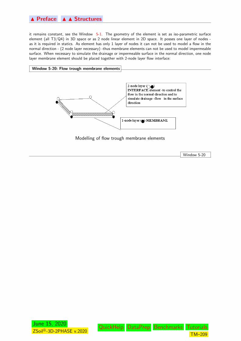
N Preface N N Structures
it remains constant, see the Window 5-1. The geometry of the element is set as iso-parametric surfaceelement (all T3/Q4) in 3D space or as 2 node linear element in 2D space. It posses one layer of nodes -as it is required in statics. As element has only 1 layer of nodes it can not be used to model a flow in thenormal direction - (2 node layer necessary) -thus membrane elements can not be used to model impermeablesurface. When necessary to simulate the drainage or impermeable surface in the normal direction, one nodelayer membrane element should be placed together with 2-node layer flow interface:
Window 5-20: Flow trough membrane elements
Modelling of flow trough membrane elements
Window 5-20
June 15, 2020ZSoilr-3D-2PHASE v.2020
QuickHelp DataPrep Benchmarks TutorialsTM–209
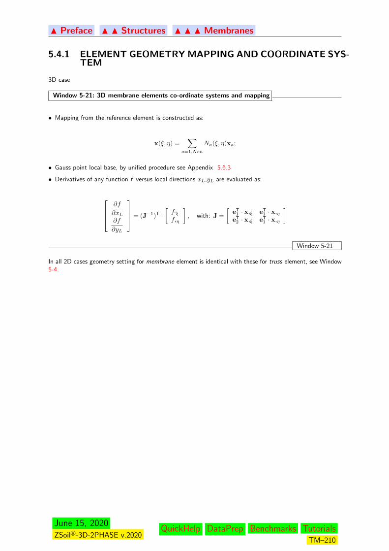
N Preface N N Structures N N N Membranes
5.4.1 ELEMENT GEOMETRY MAPPING AND COORDINATE SYS-TEM
3D case
Window 5-21: 3D membrane elements co-ordinate systems and mapping
• Mapping from the reference element is constructed as:
x(ξ, η) =∑
a=1,Nen
Na(ξ, η)xa;
• Gauss point local base, by unified procedure see Appendix 5.6.3
• Derivatives of any function f versus local directions xL,yL are evaluated as:
∂f
∂xL∂f
∂yL
= (J−1)T ·[f′ξ
f,η
], with: J =
[eT
1 · x,ξ eT1 · x,η
eT2 · x,ξ eT
1 · x,η
]
Window 5-21
In all 2D cases geometry setting for membrane element is identical with these for truss element, see Window5-4.
June 15, 2020ZSoilr-3D-2PHASE v.2020
QuickHelp DataPrep Benchmarks TutorialsTM–210
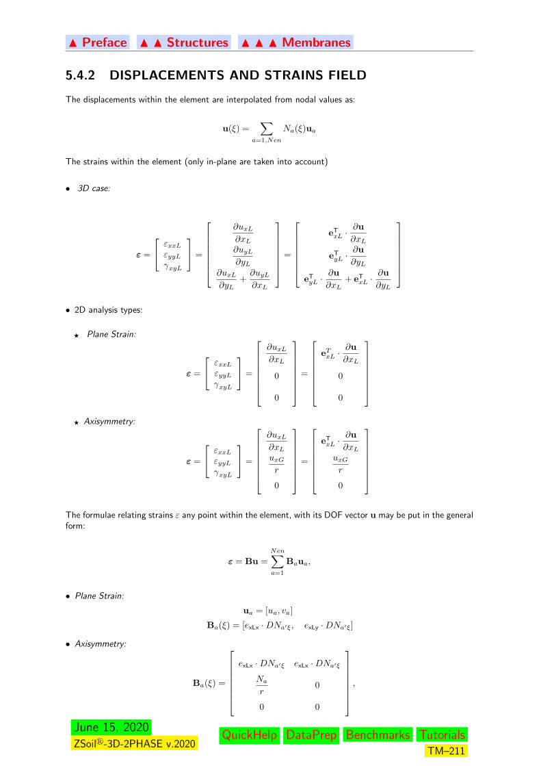
N Preface N N Structures N N N Membranes
5.4.2 DISPLACEMENTS AND STRAINS FIELD
The displacements within the element are interpolated from nodal values as:
u(ξ) =∑
a=1,Nen
Na(ξ)ua
The strains within the element (only in-plane are taken into account)
• 3D case:
ε =
εxxLεyyLγxyL
=
∂uxL∂xL∂uyL∂yL
∂uxL∂yL
+∂uyL∂xL
=
eTxL ·
∂u
∂xL
eTyL ·
∂u
∂yL
eTyL ·
∂u
∂xL+ eT
xL ·∂u
∂yL
• 2D analysis types:
F Plane Strain:
ε =
εxxLεyyLγxyL
=
∂uxL∂xL
0
0
=
eTxL ·
∂u
∂xL
0
0
F Axisymmetry:
ε =
εxxLεyyLγxyL
=
∂uxL∂xLuxGr
0
=
eTxL ·
∂u
∂xLuxGr
0
The formulae relating strains ε any point within the element, with its DOF vector u may be put in the generalform:
ε = Bu =
Nen∑a=1
Baua,
• Plane Strain:
ua = [ua, va]
Ba(ξ) = [exLx ·DNa′ξ, exLy ·DNa′ξ]
• Axisymmetry:
Ba(ξ) =
exLx ·DNa′ξ exLx ·DNa′ξ
Nar
0
0 0
,
June 15, 2020ZSoilr-3D-2PHASE v.2020
QuickHelp DataPrep Benchmarks TutorialsTM–211

N Preface N N Structures N N N Membranes
• 3D:
ua = [ua, va, wa]T
Ba(ξ, η) =
e1xNa′xL e1yNa′xL e1zNa′xL
e2xNa′yL e2yNa′yL e2zNa′yL
e1xNa′yL + e2xNa′xL e1yNa′yL + e2yNa′xL e1zNa′yL + e2zNa′xL
.
June 15, 2020ZSoilr-3D-2PHASE v.2020
QuickHelp DataPrep Benchmarks TutorialsTM–212
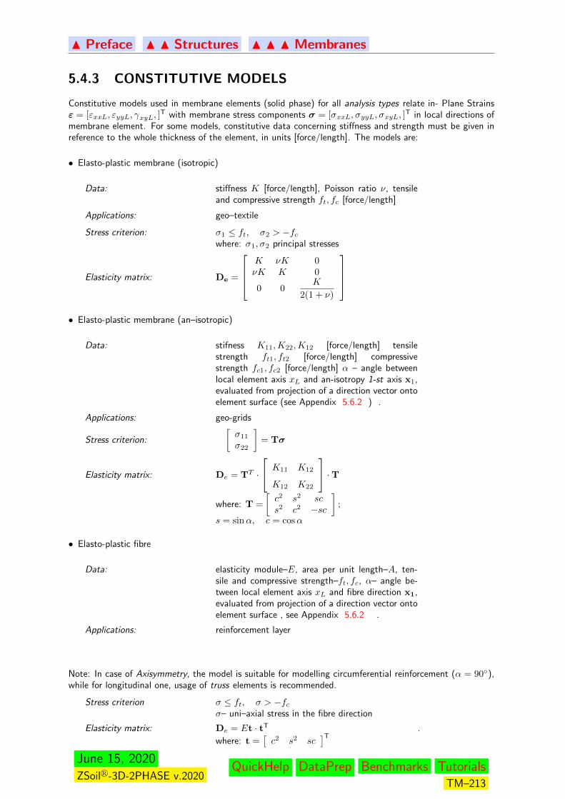
N Preface N N Structures N N N Membranes
5.4.3 CONSTITUTIVE MODELS
Constitutive models used in membrane elements (solid phase) for all analysis types relate in- Plane Strainsε = [εxxL, εyyL, γxyL, ]
T with membrane stress components σ = [σxxL, σyyL, σxyL, ]T in local directions of
membrane element. For some models, constitutive data concerning stiffness and strength must be given inreference to the whole thickness of the element, in units [force/length]. The models are:
• Elasto-plastic membrane (isotropic)
Data: stiffness K [force/length], Poisson ratio ν, tensileand compressive strength ft, fc [force/length]
Applications: geo–textile
Stress criterion: σ1 ≤ ft, σ2 > −fcwhere: σ1, σ2 principal stresses
Elasticity matrix: De =
K νK 0νK K 0
0 0K
2(1 + ν)
• Elasto-plastic membrane (an–isotropic)
Data: stifness K11,K22,K12 [force/length] tensilestrength ft1, ft2 [force/length] compressivestrength fc1, fc2 [force/length] α – angle betweenlocal element axis xL and an-isotropy 1-st axis x1,evaluated from projection of a direction vector ontoelement surface (see Appendix 5.6.2 ) .
Applications: geo-grids
Stress criterion:
[σ11
σ22
]= Tσ
Elasticity matrix: De = TT ·
K11 K12
K12 K22
·Twhere: T =
[c2 s2 scs2 c2 −sc
];
s = sinα, c = cosα
• Elasto-plastic fibre
Data: elasticity module–E, area per unit length–A, ten-sile and compressive strength–ft, fc, α– angle be-tween local element axis xL and fibre direction x1,evaluated from projection of a direction vector ontoelement surface , see Appendix 5.6.2 .
Applications: reinforcement layer
Note: In case of Axisymmetry, the model is suitable for modelling circumferential reinforcement (α = 90),while for longitudinal one, usage of truss elements is recommended.
Stress criterion σ ≤ ft, σ > −fcσ– uni–axial stress in the fibre direction
Elasticity matrix: De = Et · tT
where: t =[c2 s2 sc
]T .
June 15, 2020ZSoilr-3D-2PHASE v.2020
QuickHelp DataPrep Benchmarks TutorialsTM–213

N Preface N N Structures N N N Membranes
• Elasto plastic-plane stress member
Data: elasticity module–E, Poisson ratio ν, area per unitlength–A, Menetrey–Willam criterion data
Applications: thin lining (steel, concrete, etc.)
Stress criterion Menetrey–Willam (plane stress)
Elasticity matrix: standard plane stress
June 15, 2020ZSoilr-3D-2PHASE v.2020
QuickHelp DataPrep Benchmarks TutorialsTM–214

N Preface N N Structures N N N Membranes
5.4.4 WEAK FORMULATION OF EQUILIBRIUM
The contribution of the membrane elements to the virtual work principle expressing equilibrium of a systemmay be put as:
find σ such that:
for any δε, δu ∫S
δεTσ AdS −∫S
δuTp dS = 0
withε =
[εxxL, εyyL, γxyL,
]T;
σ = [σxxL, σyyL, σxyL, ]T
;
u =
[u v]
T for Plane Strain, Axisymmetry
[u v w]T for Gen. plane strain, 3D
A– thickness of the element (= 1 for models using membrane forces instead of stresses).
Integrals are taken over the surface of the element. S is an area attributed to the assumed computationaldomain i.e. to the unit slice for the Plane Strain or to the whole circumference for the Axisymmetric case.
June 15, 2020ZSoilr-3D-2PHASE v.2020
QuickHelp DataPrep Benchmarks TutorialsTM–215
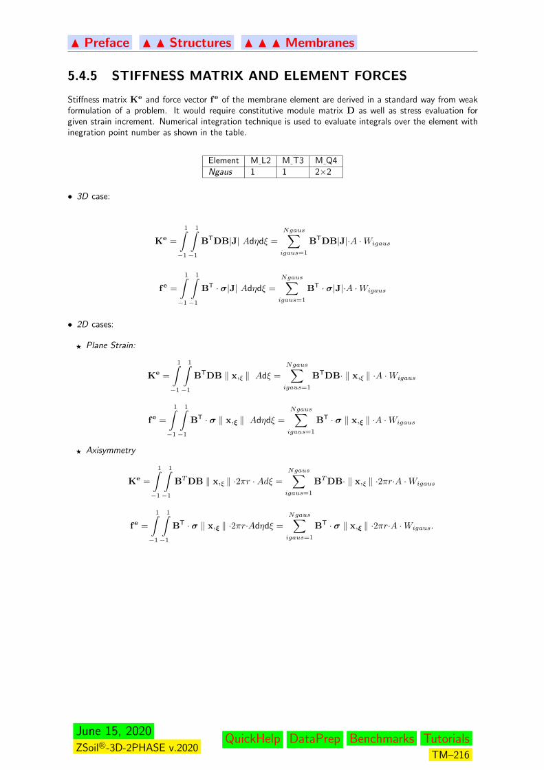
N Preface N N Structures N N N Membranes
5.4.5 STIFFNESS MATRIX AND ELEMENT FORCES
Stiffness matrix Ke and force vector fe of the membrane element are derived in a standard way from weakformulation of a problem. It would require constitutive module matrix D as well as stress evaluation forgiven strain increment. Numerical integration technique is used to evaluate integrals over the element withinegration point number as shown in the table.
Element M L2 M T3 M Q4Ngaus 1 1 2×2
• 3D case:
Ke =
1∫−1
1∫−1
BTDB|J| Adηdξ =
Ngaus∑igaus=1
BTDB|J|·A ·Wigaus
fe =
1∫−1
1∫−1
BT · σ|J| Adηdξ =
Ngaus∑igaus=1
BT · σ|J|·A ·Wigaus
• 2D cases:
F Plane Strain:
Ke =
1∫−1
1∫−1
BTDB ‖ x,ξ ‖ Adξ =
Ngaus∑igaus=1
BTDB· ‖ x,ξ ‖ ·A ·Wigaus
fe =
1∫−1
1∫−1
BT · σ ‖ x,ξ ‖ Adηdξ =
Ngaus∑igaus=1
BT · σ ‖ x,ξ ‖ ·A ·Wigaus
F Axisymmetry
Ke =
1∫−1
1∫−1
BTDB ‖ x,ξ ‖ ·2πr ·Adξ =
Ngaus∑igaus=1
BTDB· ‖ x,ξ ‖ ·2πr·A ·Wigaus
fe =
1∫−1
1∫−1
BT · σ ‖ x,ξ ‖ ·2πr·Adηdξ =
Ngaus∑igaus=1
BT · σ ‖ x,ξ ‖ ·2πr·A ·Wigaus.
June 15, 2020ZSoilr-3D-2PHASE v.2020
QuickHelp DataPrep Benchmarks TutorialsTM–216

N Preface N N Structures
5.5 NONLINEAR HINGES
NONLINEAR BEAM HINGES
NONLINEAR SHELL HINGES
Nonlinear hinge elements can be used to model complex behavior of a beam-beam or shell-shell connections.These hinge elements may be used in the uncoupled form for each specific degree of freedom (defined inlocal coordinate system) (to model no tension condition for instance)or in the coupled one (using Janssenformula) where the current bending moment may strongly depend on the axial(for beams) or membrane (forshells) force. Uncoupled/coupled hinge models (different for each degree of freedom) can be mixed withinone hinge element.
June 15, 2020ZSoilr-3D-2PHASE v.2020
QuickHelp DataPrep Benchmarks TutorialsTM–217
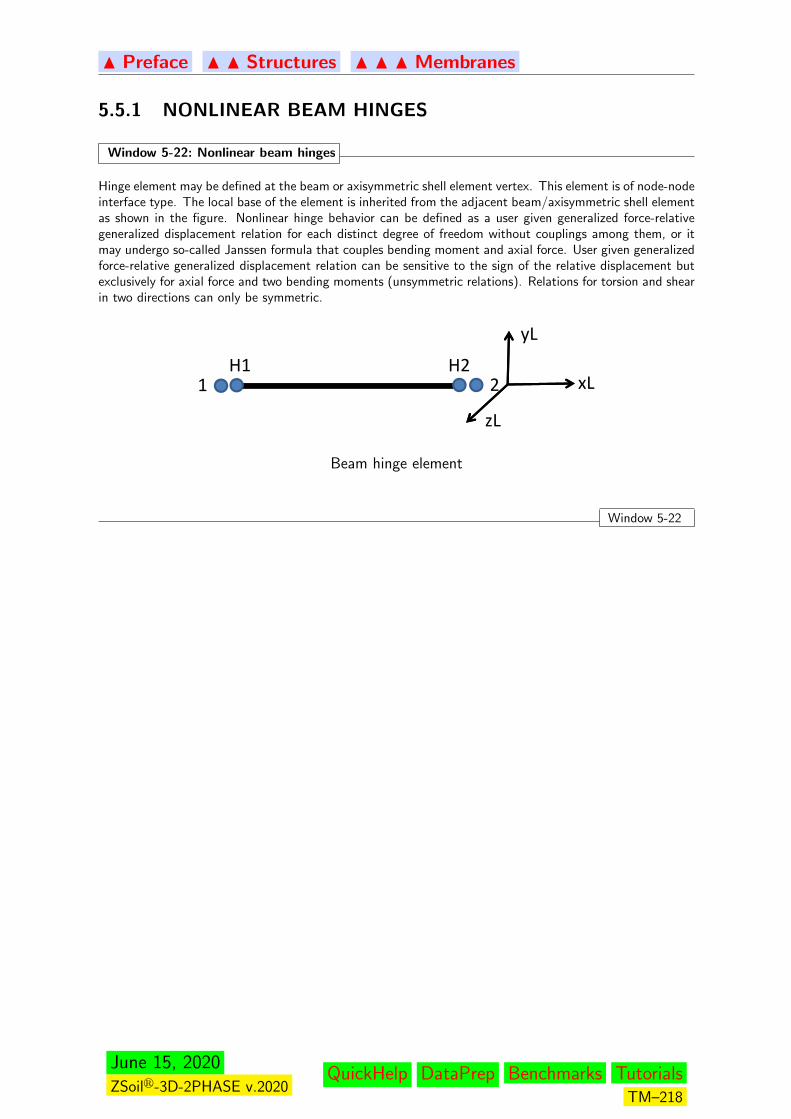
N Preface N N Structures N N N Membranes
5.5.1 NONLINEAR BEAM HINGES
Window 5-22: Nonlinear beam hinges
Hinge element may be defined at the beam or axisymmetric shell element vertex. This element is of node-nodeinterface type. The local base of the element is inherited from the adjacent beam/axisymmetric shell elementas shown in the figure. Nonlinear hinge behavior can be defined as a user given generalized force-relativegeneralized displacement relation for each distinct degree of freedom without couplings among them, or itmay undergo so-called Janssen formula that couples bending moment and axial force. User given generalizedforce-relative generalized displacement relation can be sensitive to the sign of the relative displacement butexclusively for axial force and two bending moments (unsymmetric relations). Relations for torsion and shearin two directions can only be symmetric.
yL
1 2H1 H2
xL
zLzL
Beam hinge element
Window 5-22
June 15, 2020ZSoilr-3D-2PHASE v.2020
QuickHelp DataPrep Benchmarks TutorialsTM–218
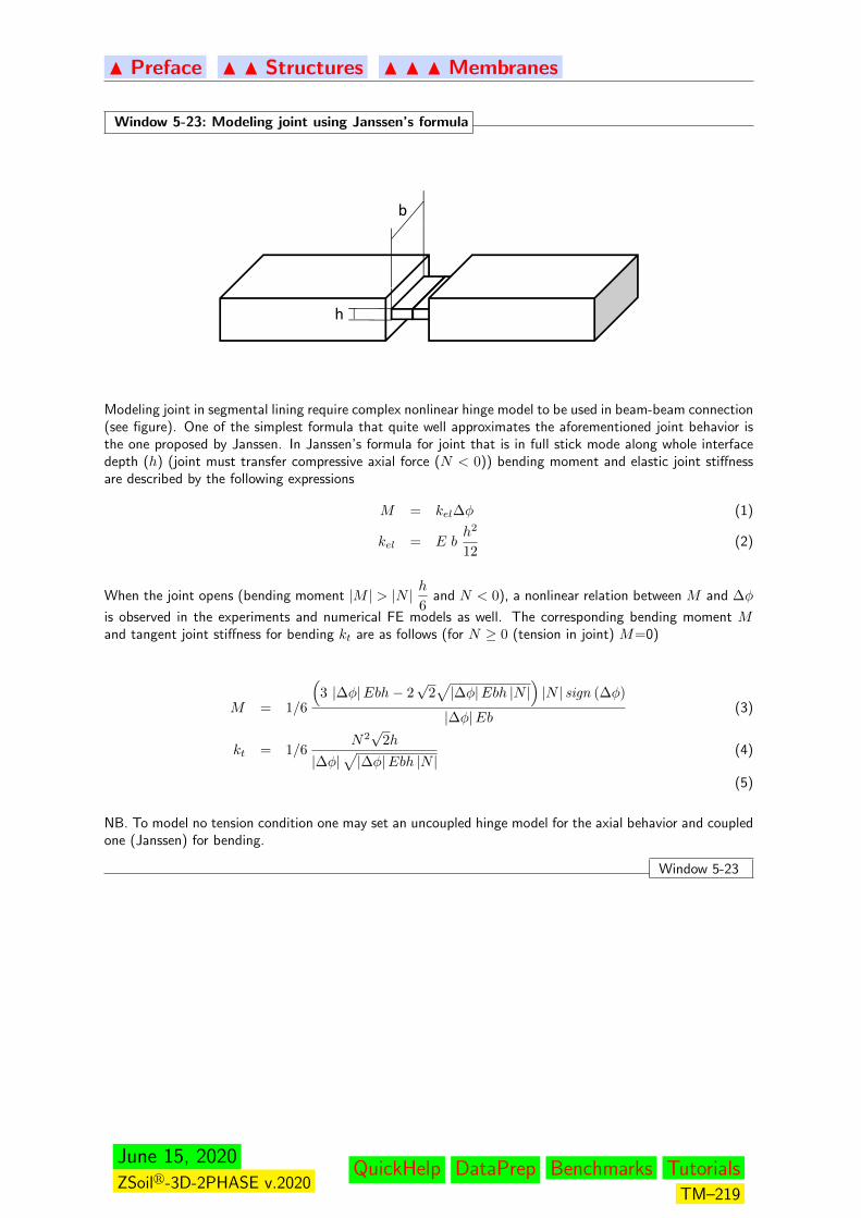
N Preface N N Structures N N N Membranes
Window 5-23: Modeling joint using Janssen’s formula
b
h
h
1m
h
Modeling joint in segmental lining require complex nonlinear hinge model to be used in beam-beam connection(see figure). One of the simplest formula that quite well approximates the aforementioned joint behavior isthe one proposed by Janssen. In Janssen’s formula for joint that is in full stick mode along whole interfacedepth (h) (joint must transfer compressive axial force (N < 0)) bending moment and elastic joint stiffnessare described by the following expressions
M = kel∆φ (1)
kel = E bh2
12(2)
When the joint opens (bending moment |M | > |N | h6
and N < 0), a nonlinear relation between M and ∆φ
is observed in the experiments and numerical FE models as well. The corresponding bending moment Mand tangent joint stiffness for bending kt are as follows (for N ≥ 0 (tension in joint) M=0)
M = 1/6
(3 |∆φ|Ebh− 2
√2√|∆φ|Ebh |N |
)|N | sign (∆φ)
|∆φ|Eb(3)
kt = 1/6N2√
2h
|∆φ|√|∆φ|Ebh |N |
(4)
(5)
NB. To model no tension condition one may set an uncoupled hinge model for the axial behavior and coupledone (Janssen) for bending.
Window 5-23
June 15, 2020ZSoilr-3D-2PHASE v.2020
QuickHelp DataPrep Benchmarks TutorialsTM–219
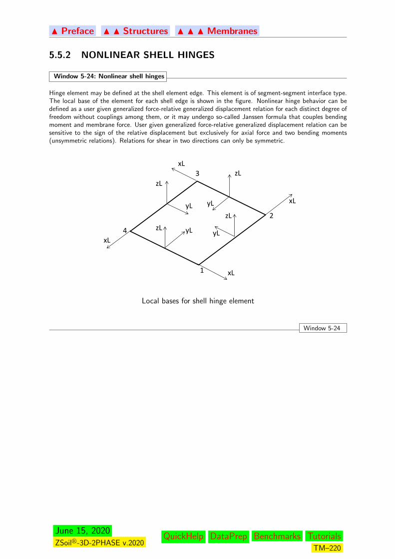
N Preface N N Structures N N N Membranes
5.5.2 NONLINEAR SHELL HINGES
Window 5-24: Nonlinear shell hinges
Hinge element may be defined at the shell element edge. This element is of segment-segment interface type.The local base of the element for each shell edge is shown in the figure. Nonlinear hinge behavior can bedefined as a user given generalized force-relative generalized displacement relation for each distinct degree offreedom without couplings among them, or it may undergo so-called Janssen formula that couples bendingmoment and membrane force. User given generalized force-relative generalized displacement relation can besensitive to the sign of the relative displacement but exclusively for axial force and two bending moments(unsymmetric relations). Relations for shear in two directions can only be symmetric.
3xL
zL
xLyL
zL
yL2
4 yL
zL
xL
y
yLzL
1
xL
1 xL
Local bases for shell hinge element
Window 5-24
June 15, 2020ZSoilr-3D-2PHASE v.2020
QuickHelp DataPrep Benchmarks TutorialsTM–220

N Preface N N Structures N N N Membranes
Window 5-25: Modeling joint using Janssen’s formula
b
h
h
1m
h
Modeling joints in segmental lining require complex nonlinear hinge model to be used in shell-shell connection(see figure). One of the simplest formula that quite well approximates the aforementioned joint behavior isthe one proposed by Janssen. In Janssen’s formula for joint that is in full stick mode along whole interfacedepth (h) (joint must transfer compressive membrane force (N < 0)) bending moment and elastic jointstiffness are described by the following expressions (same as for the beam hinge but b = 1m)
M = kel∆φ (1)
kel = Eh2
12(2)
When the joint opens (bending moment |M | > |N | h6
and N < 0), a nonlinear relation between M and ∆φ
is observed in the experiments and numerical FE models as well. The corresponding bending moment Mand tangent joint stiffness for bending kt are as follows (for N ≥ 0 (tension in joint) M=0)
M = 1/6
(3 |∆φ|Eh− 2
√2√|∆φ|Eh |N |
)|N | sign (∆φ)
|∆φ|E(3)
kt = 1/6N2√
2h
|∆φ|√|∆φ|Eh |N |
(4)
(5)
NB. To model no tension condition one may set an uncoupled hinge model for the axial behavior and coupledone (Janssen) for bending.
Window 5-25
June 15, 2020ZSoilr-3D-2PHASE v.2020
QuickHelp DataPrep Benchmarks TutorialsTM–221

N Preface N N Structures N N N Appendices
5.6 APPENDICES
MASTER-SLAVE (OFFSET) TRANSFORMATION
SETTING THE DIRECTION ON SURFACE ELEMENTS
SETTING OF THE LOCAL BASE ON A SURFACE ELEMENT
UNI-AXIAL ELASTO-PLASTIC MODEL
UNI-AXIAL USER DEFINED MODEL
June 15, 2020ZSoilr-3D-2PHASE v.2020
QuickHelp DataPrep Benchmarks TutorialsTM–222
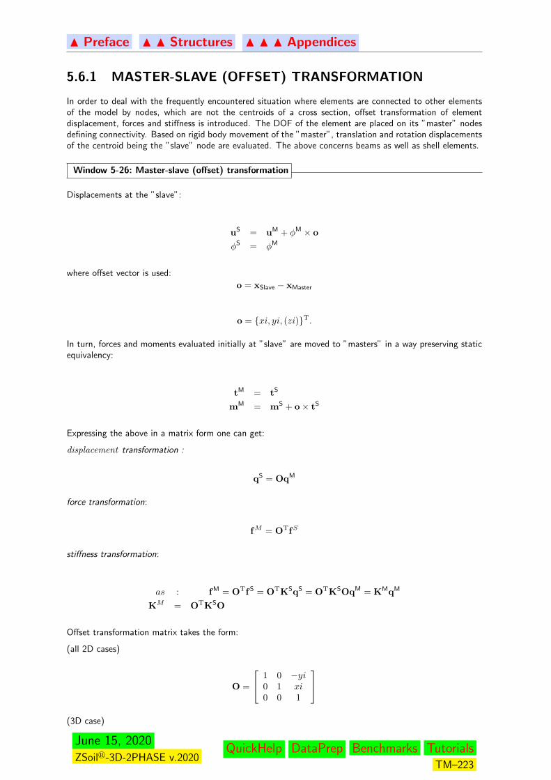
N Preface N N Structures N N N Appendices
5.6.1 MASTER-SLAVE (OFFSET) TRANSFORMATION
In order to deal with the frequently encountered situation where elements are connected to other elementsof the model by nodes, which are not the centroids of a cross section, offset transformation of elementdisplacement, forces and stiffness is introduced. The DOF of the element are placed on its ”master” nodesdefining connectivity. Based on rigid body movement of the ”master”, translation and rotation displacementsof the centroid being the ”slave” node are evaluated. The above concerns beams as well as shell elements.
Window 5-26: Master-slave (offset) transformation
Displacements at the ”slave”:
uS = uM + φM × o
φS = φM
where offset vector is used:
o = xSlave − xMaster
o = xi, yi, (zi)T.
In turn, forces and moments evaluated initially at ”slave” are moved to ”masters” in a way preserving staticequivalency:
tM = tS
mM = mS + o× tS
Expressing the above in a matrix form one can get:
displacement transformation :
qS = OqM
force transformation:
fM = OTfS
stiffness transformation:
as : fM = OTfS = OTKSqS = OTKSOqM = KMqM
KM = OTKSO
Offset transformation matrix takes the form:
(all 2D cases)
O =
1 0 −yi0 1 xi0 0 1
(3D case)
June 15, 2020ZSoilr-3D-2PHASE v.2020
QuickHelp DataPrep Benchmarks TutorialsTM–223

N Preface N N Structures N N N Appendices
O =
1 0 0 0 zi −yi0 1 0 −zi 0 xi0 0 1 yi −xi 00 0 0 1 0 00 0 0 0 1 00 0 0 0 0 1
Window 5-26
June 15, 2020ZSoilr-3D-2PHASE v.2020
QuickHelp DataPrep Benchmarks TutorialsTM–224
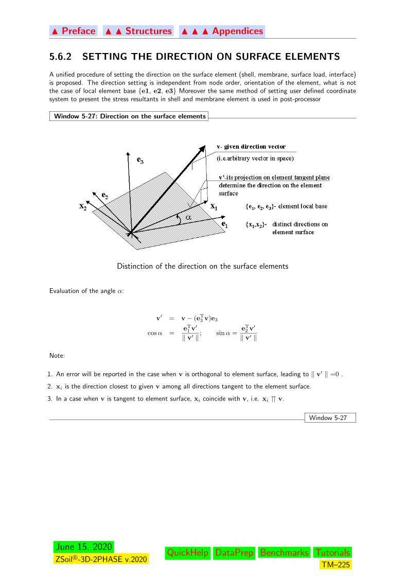
N Preface N N Structures N N N Appendices
5.6.2 SETTING THE DIRECTION ON SURFACE ELEMENTS
A unified procedure of setting the direction on the surface element (shell, membrane, surface load, interface)is proposed. The direction setting is independent from node order, orientation of the element, what is notthe case of local element base e1, e2, e3 Moreover the same method of setting user defined coordinatesystem to present the stress resultants in shell and membrane element is used in post-processor
Window 5-27: Direction on the surface elements
Distinction of the direction on the surface elements
Evaluation of the angle α:
v′ = v − (eT3 v)e3
cosα =eT
1 v′
‖ v′ ‖; sinα =
eT2 v′
‖ v′ ‖
Note:
1. An error will be reported in the case when v is orthogonal to element surface, leading to ‖ v′ ‖ =0 .
2. xi is the direction closest to given v among all directions tangent to the element surface.
3. In a case when v is tangent to element surface, xi coincide with v, i.e. xi v.
Window 5-27
June 15, 2020ZSoilr-3D-2PHASE v.2020
QuickHelp DataPrep Benchmarks TutorialsTM–225
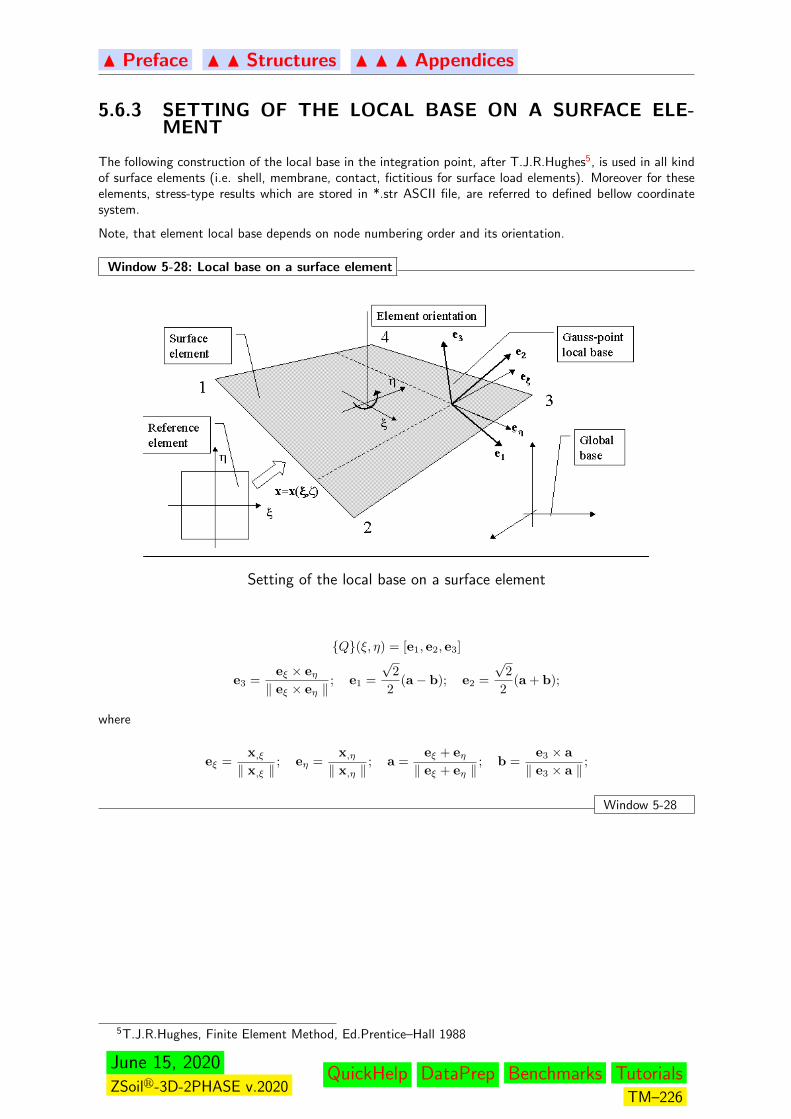
N Preface N N Structures N N N Appendices
5.6.3 SETTING OF THE LOCAL BASE ON A SURFACE ELE-MENT
The following construction of the local base in the integration point, after T.J.R.Hughes5, is used in all kindof surface elements (i.e. shell, membrane, contact, fictitious for surface load elements). Moreover for theseelements, stress-type results which are stored in *.str ASCII file, are referred to defined bellow coordinatesystem.
Note, that element local base depends on node numbering order and its orientation.
Window 5-28: Local base on a surface element
Setting of the local base on a surface element
Q(ξ, η) = [e1, e2, e3]
e3 =eξ × eη‖ eξ × eη ‖
; e1 =
√2
2(a− b); e2 =
√2
2(a + b);
where
eξ =x,ξ‖ x,ξ ‖
; eη =x,η‖ x,η ‖
; a =eξ + eη‖ eξ + eη ‖
; b =e3 × a
‖ e3 × a ‖;
Window 5-28
5T.J.R.Hughes, Finite Element Method, Ed.Prentice–Hall 1988
June 15, 2020ZSoilr-3D-2PHASE v.2020
QuickHelp DataPrep Benchmarks TutorialsTM–226
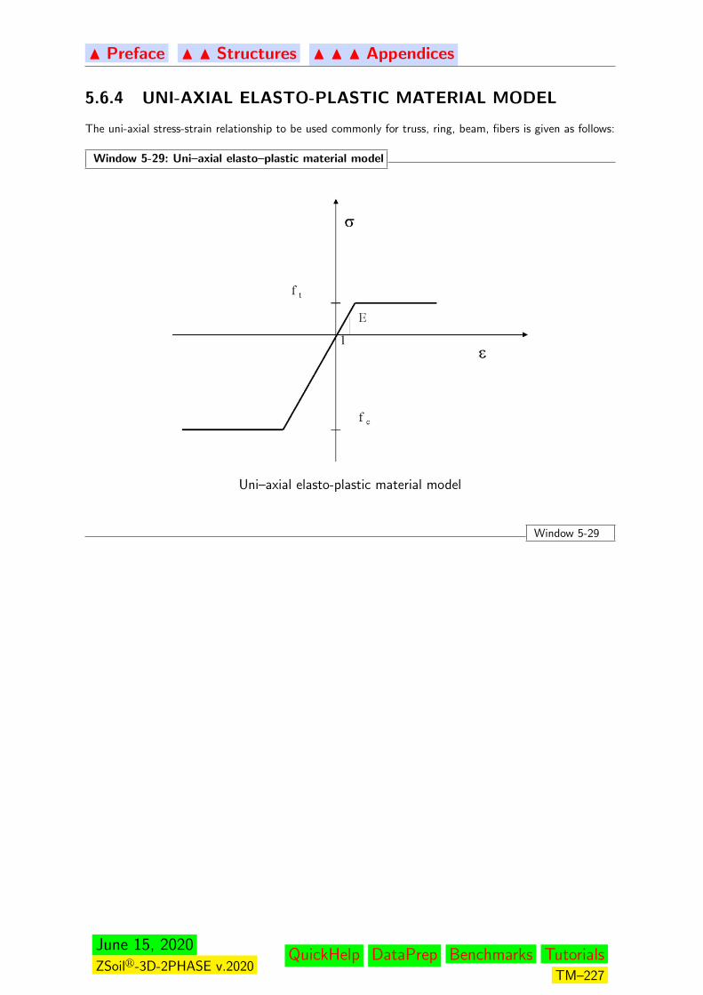
N Preface N N Structures N N N Appendices
5.6.4 UNI-AXIAL ELASTO-PLASTIC MATERIAL MODEL
The uni-axial stress-strain relationship to be used commonly for truss, ring, beam, fibers is given as follows:
Window 5-29: Uni–axial elasto–plastic material model
Uni–axial elasto-plastic material model
Window 5-29
June 15, 2020ZSoilr-3D-2PHASE v.2020
QuickHelp DataPrep Benchmarks TutorialsTM–227
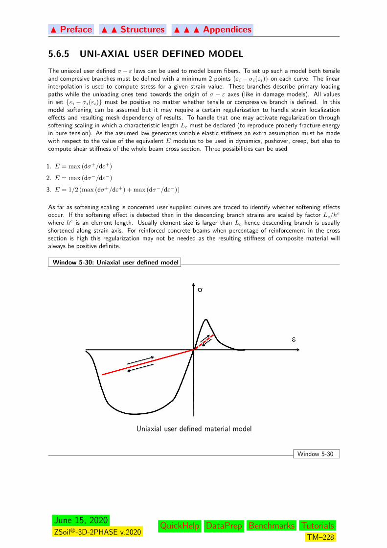
N Preface N N Structures N N N Appendices
5.6.5 UNI-AXIAL USER DEFINED MODEL
The uniaxial user defined σ− ε laws can be used to model beam fibers. To set up such a model both tensileand compresive branches must be defined with a minimum 2 points εi − σi(εi) on each curve. The linearinterpolation is used to compute stress for a given strain value. These branches describe primary loadingpaths while the unloading ones tend towards the origin of σ − ε axes (like in damage models). All valuesin set εi − σi(εi) must be positive no matter whether tensile or compressive branch is defined. In thismodel softening can be assumed but it may require a certain regularization to handle strain localizationeffects and resulting mesh dependency of results. To handle that one may activate regularization throughsoftening scaling in which a characteristic length Lc must be declared (to reproduce properly fracture energyin pure tension). As the assumed law generates variable elastic stiffness an extra assumption must be madewith respect to the value of the equivalent E modulus to be used in dynamics, pushover, creep, but also tocompute shear stiffness of the whole beam cross section. Three possibilities can be used
1. E = max (dσ+/dε+)
2. E = max (dσ−/dε−)
3. E = 1/2 (max (dσ+/dε+) + max (dσ−/dε−))
As far as softening scaling is concerned user supplied curves are traced to identify whether softening effectsoccur. If the softening effect is detected then in the descending branch strains are scaled by factor Lc/h
e
where he is an element length. Usually element size is larger than Lc hence descending branch is usuallyshortened along strain axis. For reinforced concrete beams when percentage of reinforcement in the crosssection is high this regularization may not be needed as the resulting stiffness of composite material willalways be positive definite.
Window 5-30: Uniaxial user defined model
Uniaxial user defined material model
Window 5-30
June 15, 2020ZSoilr-3D-2PHASE v.2020
QuickHelp DataPrep Benchmarks TutorialsTM–228

N Preface
Chapter 6
INTERFACE
CONTACT
PILE INTERFACE
PILE TIP INTERFACE
June 15, 2020ZSoilr-3D-2PHASE v.2020
QuickHelp DataPrep Benchmarks TutorialsTM–229

N Preface N N Interface
6.1 CONTACT OF SOLIDS AND FLUID INTERFACE
GENERAL OUTLOOK
DISPLACEMENT & STRAINS
CONSTITUTIVE MODEL
STIFFNESS MATRIX AND FORCE VECTOR
AUGMENTED LAGRANGIAN APPROACH
CONTRIBUTION TO CONTINUITY EQUATION
June 15, 2020ZSoilr-3D-2PHASE v.2020
QuickHelp DataPrep Benchmarks TutorialsTM–230

N Preface N N Interface N N Contact
6.1.1 GENERAL OUTLOOK
Window 6-1: Interface elements: General remarks
Mechanical contact as well as flux (of fluid, heat, humidity) through the surface between two bodies ismodelled by finite element discretization of the interface between them. The interface elements use nodesbelonging to the FE–mesh of both adjacent solids with assumed invariable topology (small displacementtheory). Moreover the compatibility of the initial positions of nodes is required (this is assured by pre–processing tools, see Interface option).
Interface (contact) elements between 2 adjacent bodies
Interface element geometry is based on the iso-parametric mapping from the reference element. As nodes ofboth layers of element are assumed to occupy the same position :
x(ξ) =∑
i=1,..,Nen
Ni(ξ)xi.
Family of interface elements
Window 6-1
June 15, 2020ZSoilr-3D-2PHASE v.2020
QuickHelp DataPrep Benchmarks TutorialsTM–231

N Preface N N Interface N N Contact
Window 6-2: Interface: Mechanical contact
As an additional feature, for mechanical contact, the displacements continuity option is introduced. This isrelated to interface element status.
Status CONTACT: The interface elements reproduce the force action between the two bodies based on therelative displacements of the interface nodes. The elasto–plastic friction model is used, allowing for slidingand separation, while the elastic properties of the interface impose penalty constraints multipliers excludingpenetration, see Window 6-4 for the details.
Status CONTINUITY(u,p,T) or CONTINUITY(u,T): Displacements continuity across the interface isenforced. Nodes on both sides of the interface share the same kinematical DOFs.
Window 6-2
Window 6-3: Fluid Phase
In case of Flow or Deformation+Flow analysis mode, interface elements may posses pressure DOF at nodesof both layers. Interface elements can be used to model following situations:
Fully permeable interface
Pressures continuity across the interface is enforced. Nodes on both sides of the interface share the samepressure DOFs.
Impermeable interface
No flow takes place in the direction normal to the interface (”no flux” qn = 0 condition on both faces isimposed). Resulting pressures on both interface faces will be (in general) discontinuos. In this case theinterface element does not contribute to the equation system.
Permeable interface
Both isotropic and anisotropic flow conditions can be handled.
Window 6-3
June 15, 2020ZSoilr-3D-2PHASE v.2020
QuickHelp DataPrep Benchmarks TutorialsTM–232
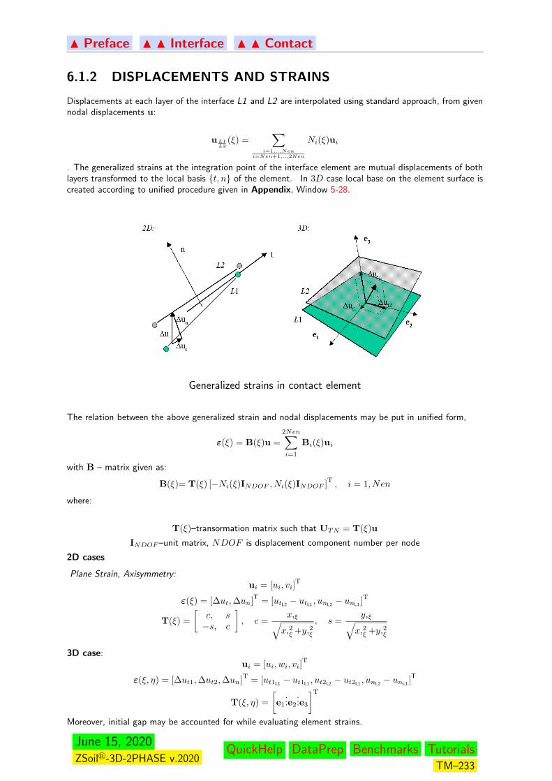
N Preface N N Interface N N Contact
6.1.2 DISPLACEMENTS AND STRAINS
Displacements at each layer of the interface L1 and L2 are interpolated using standard approach, from givennodal displacements u:
uL1L2
(ξ) =∑
i=1,..,Neni=Nen+1,..,2Nen
Ni(ξ)ui
. The generalized strains at the integration point of the interface element are mutual displacements of bothlayers transformed to the local basis t, n of the element. In 3D case local base on the element surface iscreated according to unified procedure given in Appendix, Window 5-28.
Generalized strains in contact element
The relation between the above generalized strain and nodal displacements may be put in unified form,
ε(ξ) = B(ξ)u =
2Nen∑i=1
Bi(ξ)ui
with B – matrix given as:
B(ξ)= T(ξ) [−Ni(ξ)INDOF , Ni(ξ)INDOF ]T, i = 1, Nen
where:
T(ξ)–transormation matrix such that UTN = T(ξ)u
INDOF –unit matrix, NDOF is displacement component number per node
2D cases
Plane Strain, Axisymmetry:ui = [ui, vi]
T
ε(ξ) = [∆ut,∆un]T
= [utL2− utL1
, unL2− unL1
]T
T(ξ) =
[c, s−s, c
], c =
x,ξ√x,2ξ +y,2ξ
, s =y,ξ√x,2ξ +y,2ξ
3D case:ui = [ui, wi, vi]
T
ε(ξ, η) = [∆ut1,∆ut2,∆un]T
= [ut1L1− ut1L1
, ut2L2− ut2L1
, unL2− unL1
]T
T(ξ, η) =
[e1
...e2
...e3
]T
Moreover, initial gap may be accounted for while evaluating element strains.
June 15, 2020ZSoilr-3D-2PHASE v.2020
QuickHelp DataPrep Benchmarks TutorialsTM–233
N Preface N N Interface N N Contact
6.1.3 CONSTITUTIVE MODEL
Constitutive behavior of the interface is described in the terms of:
• generalized strains ε, evaluated from nodal displacements of the interface
• effective stresses σ′, submitted to appropriate stress criterions resulting from
1. cohesive Mohr - Coulomb condition
2. no-tension condition.
For Plane Strain and Axisymmetry number of stress components Nstre = 2, while for 3D analysis Nstre =3. In the case of analysis mode Deformation+Flow, the concept of effective stress is used taking into accountpressures p and saturation ratio S:
Nstre = 2 Nstre = 3
σ = σ′ + S
[0p
]σ = σ′ + S
00p
• flow rule with a flow potential in the form analogous to Mohr-Coulomb yield function allowing for non-
associative flow rule in the case when φ 6= ψ,
• constitutive matrix D.
Both σ′ and D are evaluated within the frame of perfect multi–surface elasto–plasticity theory, with com-ponents related to the plane of the interface and its normal.
Formulation of both cases of contact constitutive law is given in the Window 6-4.
The trial stresses σ∗ are evaluated as:σ∗ = σn + Del∆ε
using the previous stress σn, strain increment ∆ε, the elastic (penalty) interface stiffness Del.
The elastic stiffness Kn should be large enough to prevent significant penetration in the case of compression,but can not undertake arbitrarily large values as it might spoil conditioning of the resulting FE equationsystem and lead to difficulties in obtaining convergence of the solution. Estimation of penalty stiffness isdone as follows in the Window 6-5.
June 15, 2020ZSoilr-3D-2PHASE v.2020
QuickHelp DataPrep Benchmarks TutorialsTM–234
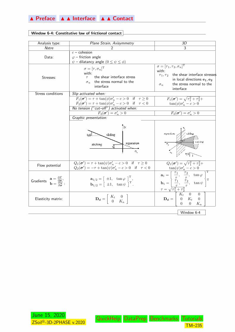
N Preface N N Interface N N Contact
Window 6-4: Constitutive law of frictional contact
Analysis type: Plane Strain, Axisymmetry 3DNstre 2 3
Data:c – cohesionϕ – friction angleψ – dilatancy angle (0 ≤ ψ ≤ φ)
Stresses:
σ = [τ , σn]T
with:τ the shear interface stressσn the stress normal to the
interface
σ = [τ1, τ2, σn]T
with:τ1, τ2 the shear interface stresses
in local directions e1, e2σn the stress normal to the
interfaceStress conditions Slip activated when:
F1(σ′) = τ + tan(φ)σ′n − c > 0 if τ ≥ 0F2(σ′) = τ + tan(φ)σ′n − c > 0 if τ < 0
F1(σ′) =√τ2
1 + τ22+
tan(φ)σ′n − c > 0No tension (”cut–off”) activated when:
F3(σ′) = σ′n > 0 F2(σ′) = σ′n > 0Graphic presentation:
Flow potentialQ1(σ′) = τ + tan(ψ)σ′n − c > 0 if τ ≥ 0Q2(σ′) = −τ + tan(ψ)σ′n − c > 0 if τ < 0
Q1(σ′) =√τ2
1 + τ22+
tan(ψ)σ′n − c > 0
Gradientsa = ∂F
∂σ ,
b = ∂Q∂σ :
a1/2 =[±1, tanϕ
]T,
b1/2 =[±1, tanψ
]T.
a1 =[ τ1
τ,
τ2
τ, tanϕ
]Tb1 =
[ τ1
τ,
τ2
τ, tanψ
]Tτ =
√τ2
1 + τ22
Elasticity matrix: Del =
[Kt 00 Kn
]Del =
Kt 0 00 Kt 00 0 Kn
Window 6-4
June 15, 2020ZSoilr-3D-2PHASE v.2020
QuickHelp DataPrep Benchmarks TutorialsTM–235
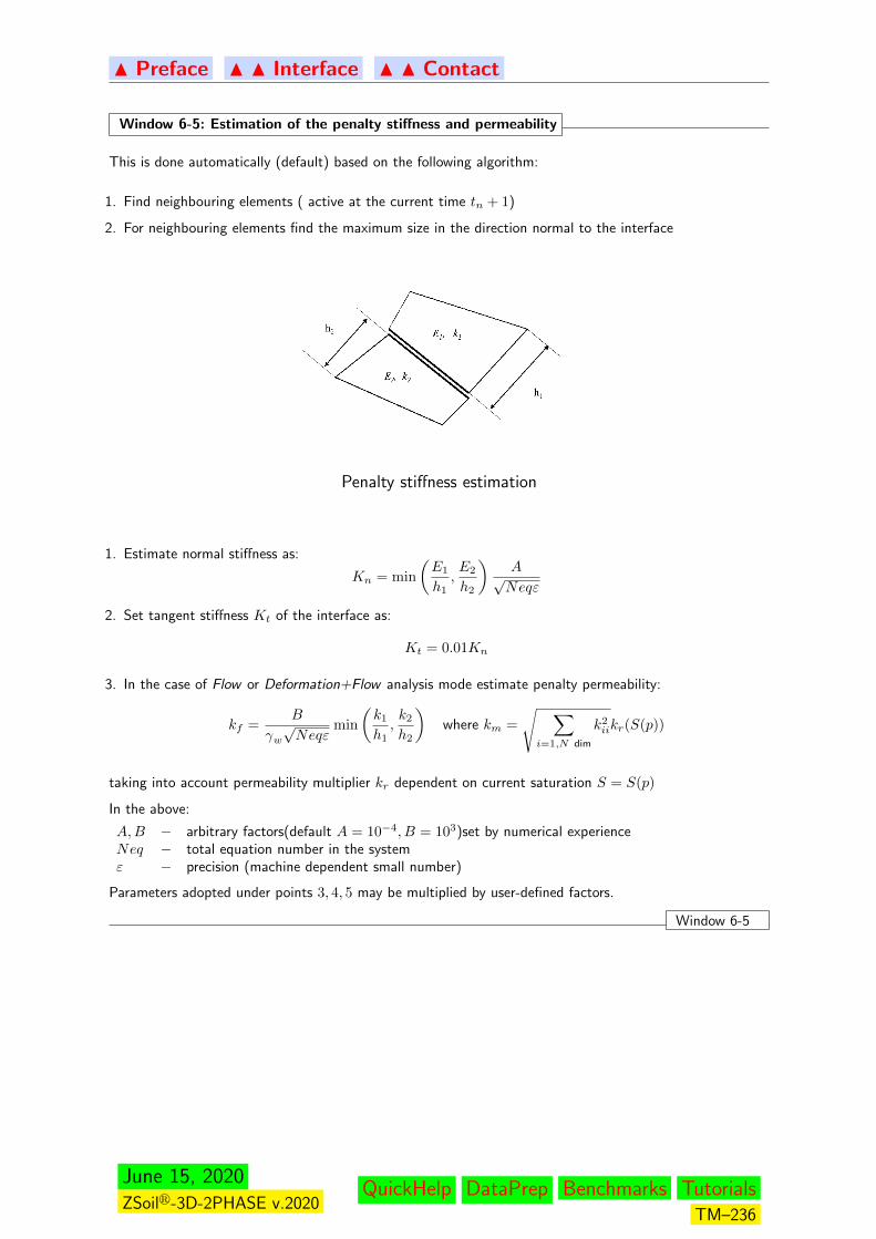
N Preface N N Interface N N Contact
Window 6-5: Estimation of the penalty stiffness and permeability
This is done automatically (default) based on the following algorithm:
1. Find neighbouring elements ( active at the current time tn + 1)
2. For neighbouring elements find the maximum size in the direction normal to the interface
Penalty stiffness estimation
1. Estimate normal stiffness as:
Kn = min
(E1
h1,E2
h2
)A√Neqε
2. Set tangent stiffness Kt of the interface as:
Kt = 0.01Kn
3. In the case of Flow or Deformation+Flow analysis mode estimate penalty permeability:
kf =B
γw√Neqε
min
(k1
h1,k2
h2
)where km =
√ ∑i=1,N dim
k2iikr(S(p))
taking into account permeability multiplier kr dependent on current saturation S = S(p)
In the above:
A,B − arbitrary factors(default A = 10−4, B = 103)set by numerical experienceNeq − total equation number in the systemε − precision (machine dependent small number)
Parameters adopted under points 3, 4, 5 may be multiplied by user-defined factors.
Window 6-5
June 15, 2020ZSoilr-3D-2PHASE v.2020
QuickHelp DataPrep Benchmarks TutorialsTM–236
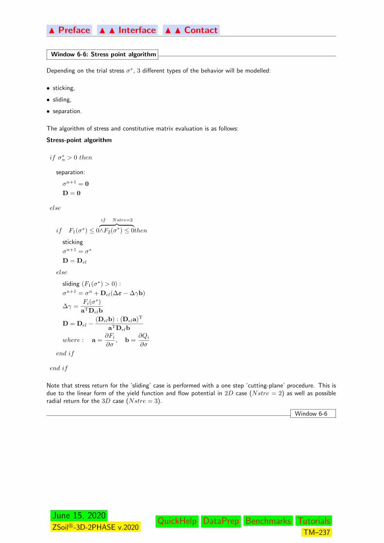
N Preface N N Interface N N Contact
Window 6-6: Stress point algorithm
Depending on the trial stress σ∗, 3 different types of the behavior will be modelled:
• sticking,
• sliding,
• separation.
The algorithm of stress and constitutive matrix evaluation is as follows:
Stress-point algorithm
if σ∗n > 0 then
separation:
σn+1 = 0
D = 0
else
if F1(σ∗) ≤ 0
if Nstre=2︷ ︸︸ ︷∧F2(σ∗) ≤ 0then
sticking
σn+1 = σ∗
D = Del
else
sliding (F1(σ∗) > 0) :
σn+1 = σn + Del(∆ε−∆γb)
∆γ =Fi(σ
∗)
aTDelb
D = Del −(Delb) : (Dela)T
aTDelb
where : a =∂Fi∂σ
, b =∂Qi∂σ
end if
end if
Note that stress return for the ’sliding’ case is performed with a one step ’cutting-plane’ procedure. This isdue to the linear form of the yield function and flow potential in 2D case (Nstre = 2) as well as possibleradial return for the 3D case (Nstre = 3).
Window 6-6
June 15, 2020ZSoilr-3D-2PHASE v.2020
QuickHelp DataPrep Benchmarks TutorialsTM–237
N Preface N N Interface N N Contact
6.1.4 STIFFNESS MATRIX AND ELEMENT FORCE VECTOR
These are evaluated as: 3D case:
Ke =
1∫−1
1∫−1
BTDB | J |dηdξ =
Ngaus∑igaus=1
BTDB | J |Wigaus
fe =
1∫−1
1∫−1
BTσ | J |dηdξ =
Ngaus∑igaus=1
BTσ | J |Wigaus
2D cases:
Plane Strain
Ke =
1∫−1
BTDB ‖ x,ξ ‖ dξ =
Ngaus∑igaus=1
BTDB ‖ x,ξ ‖Wigaus
fe =
1∫−1
BTσ ‖ x,ξ ‖ dξ =
Ngaus∑igaus=1
BTσ ‖ x,ξ ‖Wigaus
Axisymmetry
Ke =
1∫−1
BTDB ‖ x,ξ ‖ 2πrdξ =
Ngaus∑igaus=1
BTDB ‖ x,ξ ‖ 2πrWigaus
fe =
1∫−1
BTσ ‖ x,ξ ‖ 2πrdξ =
Ngaus∑igaus=1
BTσ ‖ x,ξ ‖ 2πrWigaus
with constitutive matrix D and stresses σ being the result of the point level algorithm, see Window 6.5.4 .Note that in the case of Analysis mode Deformation +Flow, the total stresses σ including pressure is usedto evaluate element forces. In order to avoid oscillatory patterns of normal stress, integration is performed atnodes and not standard Gauss points. In addition normal vectors at each node are averaged from all adjacentelements. The B matrix is evaluated as follows:
B(ξigaus) =
Bt(ξigaus)s
Bn(ξigaus)
June 15, 2020ZSoilr-3D-2PHASE v.2020
QuickHelp DataPrep Benchmarks TutorialsTM–238
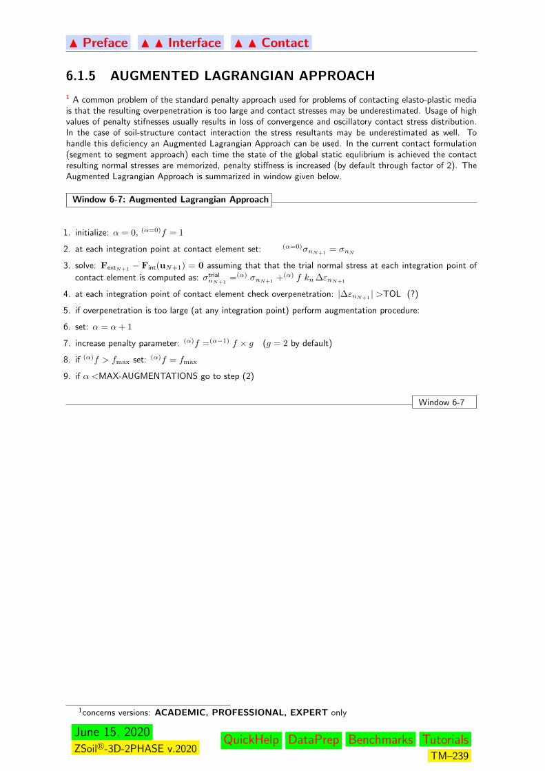
N Preface N N Interface N N Contact
6.1.5 AUGMENTED LAGRANGIAN APPROACH
1 A common problem of the standard penalty approach used for problems of contacting elasto-plastic mediais that the resulting overpenetration is too large and contact stresses may be underestimated. Usage of highvalues of penalty stifnesses usually results in loss of convergence and oscillatory contact stress distribution.In the case of soil-structure contact interaction the stress resultants may be underestimated as well. Tohandle this deficiency an Augmented Lagrangian Approach can be used. In the current contact formulation(segment to segment approach) each time the state of the global static equlibrium is achieved the contactresulting normal stresses are memorized, penalty stiffness is increased (by default through factor of 2). TheAugmented Lagrangian Approach is summarized in window given below.
Window 6-7: Augmented Lagrangian Approach
1. initialize: α = 0, (α=0)f = 1
2. at each integration point at contact element set: (α=0)σnN+1= σnN
3. solve: FextN+1− Fint(uN+1) = 0 assuming that that the trial normal stress at each integration point of
contact element is computed as: σtrialnN+1
=(α) σnN+1+(α) f kn ∆εnN+1
4. at each integration point of contact element check overpenetration: |∆εnN+1| >TOL (?)
5. if overpenetration is too large (at any integration point) perform augmentation procedure:
6. set: α = α+ 1
7. increase penalty parameter: (α)f =(α−1) f × g (g = 2 by default)
8. if (α)f > fmax set: (α)f = fmax
9. if α <MAX-AUGMENTATIONS go to step (2)
Window 6-7
1concerns versions: ACADEMIC, PROFESSIONAL, EXPERT only
June 15, 2020ZSoilr-3D-2PHASE v.2020
QuickHelp DataPrep Benchmarks TutorialsTM–239

N Preface N N Interface N N Contact
6.1.6 CONTRIBUTION TO CONTINUITY EQUATION
In the case of active fluid phase interface elements contribute to matrix H and flux vector Q (see Section4.1.2) with the following:
HInterface = −∫Γ
[N−N
]kf[NT, −NT
]dΓ
QInterface = −HInterfacetw
where:
NT =[N1(ξ) . . . NNen(ξ)
]– shape function vector
tTw =
[tw1, . . . twNen
]– nodal pressure vector.
The integration technique analogous to the one used for Stiffness matrix and element force vector evaluationis used.
June 15, 2020ZSoilr-3D-2PHASE v.2020
QuickHelp DataPrep Benchmarks TutorialsTM–240

N Preface N N Interface
6.2 PILE CONTACT INTERFACE
GENERAL OUTLOOK
DISPLACEMENT & STRAINS
CONSTITUTIVE MODEL
June 15, 2020ZSoilr-3D-2PHASE v.2020
QuickHelp DataPrep Benchmarks TutorialsTM–241
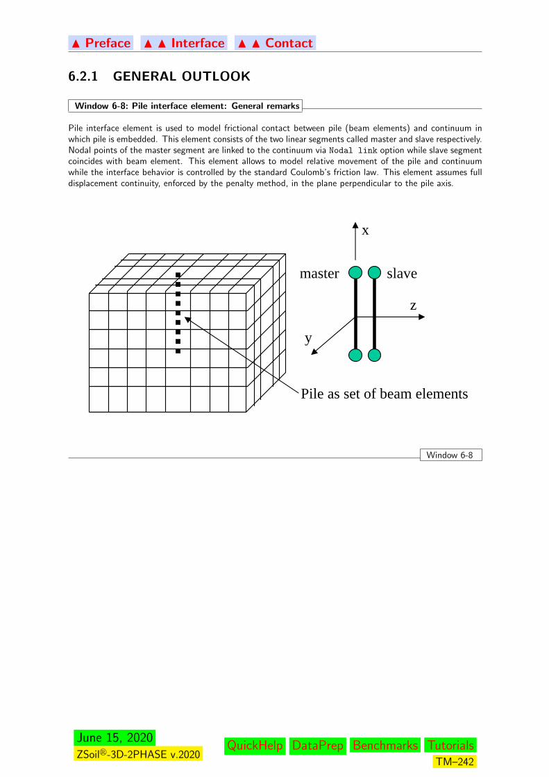
N Preface N N Interface N N Contact
6.2.1 GENERAL OUTLOOK
Window 6-8: Pile interface element: General remarks
Pile interface element is used to model frictional contact between pile (beam elements) and continuum inwhich pile is embedded. This element consists of the two linear segments called master and slave respectively.Nodal points of the master segment are linked to the continuum via Nodal link option while slave segmentcoincides with beam element. This element allows to model relative movement of the pile and continuumwhile the interface behavior is controlled by the standard Coulomb’s friction law. This element assumes fulldisplacement continuity, enforced by the penalty method, in the plane perpendicular to the pile axis.
master slave
x
y
z
Pile as set of beam elements
Window 6-8
June 15, 2020ZSoilr-3D-2PHASE v.2020
QuickHelp DataPrep Benchmarks TutorialsTM–242
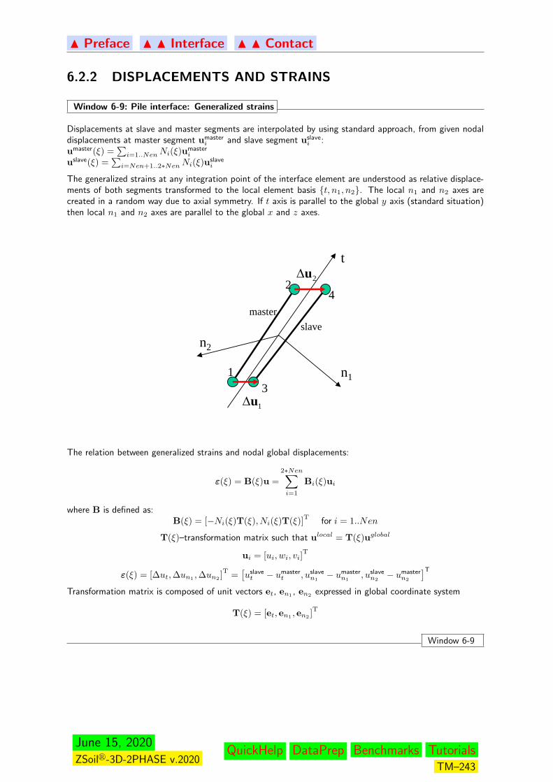
N Preface N N Interface N N Contact
6.2.2 DISPLACEMENTS AND STRAINS
Window 6-9: Pile interface: Generalized strains
Displacements at slave and master segments are interpolated by using standard approach, from given nodaldisplacements at master segment umaster
i and slave segment uslavei :
umaster(ξ) =∑i=1..NenNi(ξ)u
masteri
uslave(ξ) =∑i=Nen+1..2∗NenNi(ξ)u
slavei
The generalized strains at any integration point of the interface element are understood as relative displace-ments of both segments transformed to the local element basis t, n1, n2. The local n1 and n2 axes arecreated in a random way due to axial symmetry. If t axis is parallel to the global y axis (standard situation)then local n1 and n2 axes are parallel to the global x and z axes.
t
n1
n2
masterslave
1
2
3
4
1Δu
2Δu
The relation between generalized strains and nodal global displacements:
ε(ξ) = B(ξ)u =
2∗Nen∑i=1
Bi(ξ)ui
where B is defined as:B(ξ) = [−Ni(ξ)T(ξ), Ni(ξ)T(ξ)]
T for i = 1..Nen
T(ξ)–transformation matrix such that ulocal = T(ξ)uglobal
ui = [ui, wi, vi]T
ε(ξ) = [∆ut,∆un1,∆un2
]T
=[uslavet − umaster
t , uslaven1− umaster
n1, uslaven2− umaster
n2
]TTransformation matrix is composed of unit vectors et, en1 , en2 expressed in global coordinate system
T(ξ) = [et, en1, en2
]T
Window 6-9
June 15, 2020ZSoilr-3D-2PHASE v.2020
QuickHelp DataPrep Benchmarks TutorialsTM–243
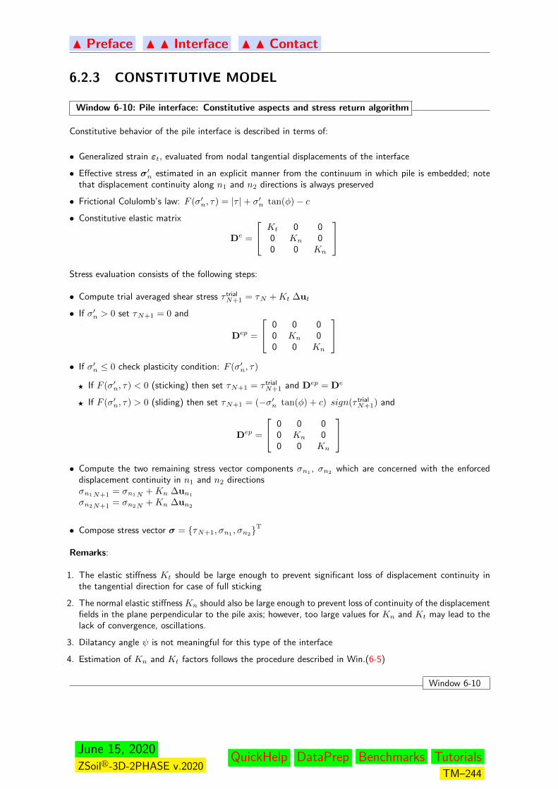
N Preface N N Interface N N Contact
6.2.3 CONSTITUTIVE MODEL
Window 6-10: Pile interface: Constitutive aspects and stress return algorithm
Constitutive behavior of the pile interface is described in terms of:
• Generalized strain εt, evaluated from nodal tangential displacements of the interface
• Effective stress σ′n estimated in an explicit manner from the continuum in which pile is embedded; notethat displacement continuity along n1 and n2 directions is always preserved
• Frictional Colulomb’s law: F (σ′n, τ) = |τ |+ σ′n tan(φ)− c
• Constitutive elastic matrix
De =
Kt 0 00 Kn 00 0 Kn
Stress evaluation consists of the following steps:
• Compute trial averaged shear stress τ trialN+1 = τN +Kt ∆ut
• If σ′n > 0 set τN+1 = 0 and
Dep =
0 0 00 Kn 00 0 Kn
• If σ′n ≤ 0 check plasticity condition: F (σ′n, τ)
F If F (σ′n, τ) < 0 (sticking) then set τN+1 = τ trialN+1 and Dep = De
F If F (σ′n, τ) > 0 (sliding) then set τN+1 = (−σ′n tan(φ) + c) sign(τ trialN+1) and
Dep =
0 0 00 Kn 00 0 Kn
• Compute the two remaining stress vector components σn1 , σn2 which are concerned with the enforced
displacement continuity in n1 and n2 directionsσn1N+1 = σn1N +Kn ∆un1
σn2N+1 = σn2N +Kn ∆un2
• Compose stress vector σ = τN+1, σn1, σn2T
Remarks:
1. The elastic stiffness Kt should be large enough to prevent significant loss of displacement continuity inthe tangential direction for case of full sticking
2. The normal elastic stiffness Kn should also be large enough to prevent loss of continuity of the displacementfields in the plane perpendicular to the pile axis; however, too large values for Kn and Kt may lead to thelack of convergence, oscillations.
3. Dilatancy angle ψ is not meaningful for this type of the interface
4. Estimation of Kn and Kt factors follows the procedure described in Win.(6-5)
Window 6-10
June 15, 2020ZSoilr-3D-2PHASE v.2020
QuickHelp DataPrep Benchmarks TutorialsTM–244

N Preface N N Interface N N Contact
6.2.4 STIFFNESS MATRIX AND ELEMENT FORCE VECTOR
Ke = 2π rpile
1∫−1
BTDB | J |dξ = 2π rpileNgaus∑igaus=1
BTDB | J |Wigaus
fe = 2π rpile
1∫−1
BTσ | J |dξ = 2π rpileNgaus∑igaus=1
BTσ | J |Wigaus
Remarks:
1. rpile is a radius of pile (reinforcement)
June 15, 2020ZSoilr-3D-2PHASE v.2020
QuickHelp DataPrep Benchmarks TutorialsTM–245

N Preface N N Interface
6.3 PILE TIP CONTACT INTERFACE
GENERAL OUTLOOK
DISPLACEMENT & STRAINS
CONSTITUTIVE MODEL
June 15, 2020ZSoilr-3D-2PHASE v.2020
QuickHelp DataPrep Benchmarks TutorialsTM–246
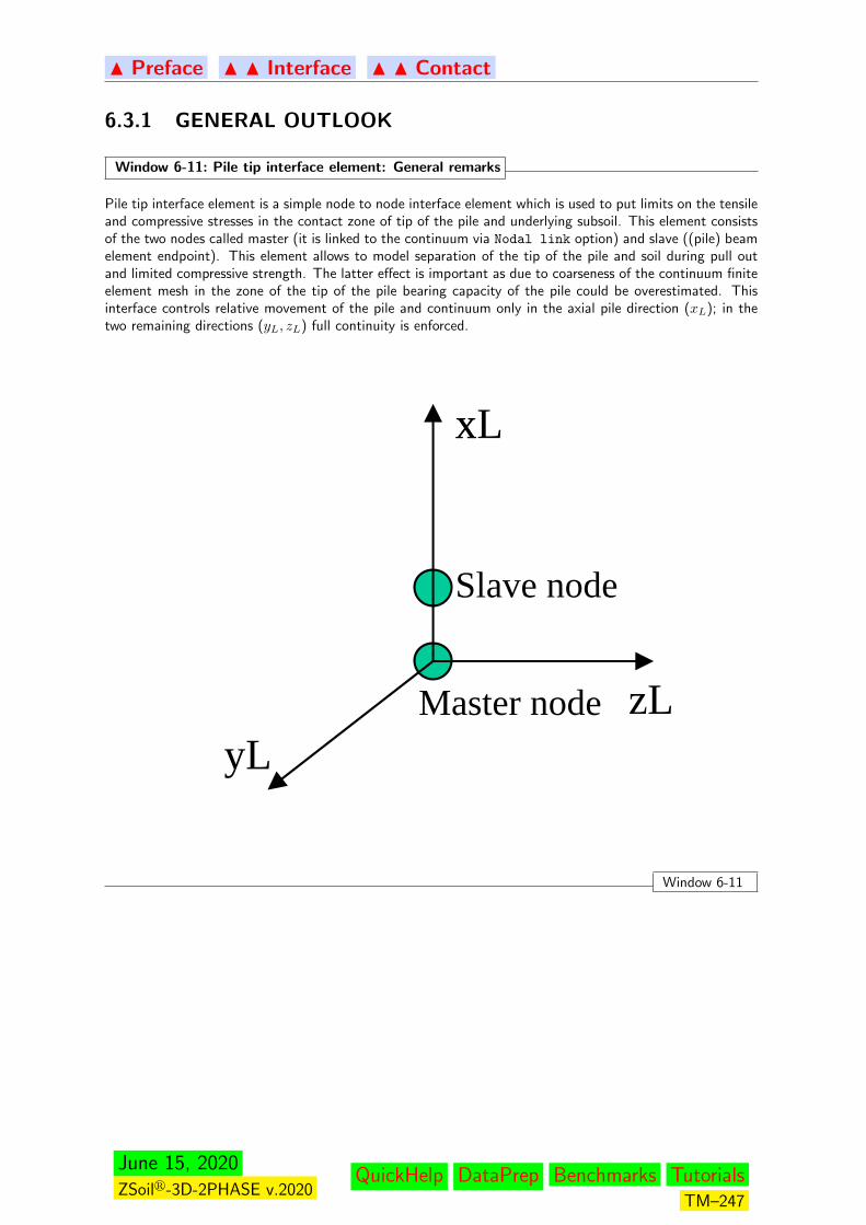
N Preface N N Interface N N Contact
6.3.1 GENERAL OUTLOOK
Window 6-11: Pile tip interface element: General remarks
Pile tip interface element is a simple node to node interface element which is used to put limits on the tensileand compressive stresses in the contact zone of tip of the pile and underlying subsoil. This element consistsof the two nodes called master (it is linked to the continuum via Nodal link option) and slave ((pile) beamelement endpoint). This element allows to model separation of the tip of the pile and soil during pull outand limited compressive strength. The latter effect is important as due to coarseness of the continuum finiteelement mesh in the zone of the tip of the pile bearing capacity of the pile could be overestimated. Thisinterface controls relative movement of the pile and continuum only in the axial pile direction (xL); in thetwo remaining directions (yL, zL) full continuity is enforced.
xL
zL
x
yL
Slave node
Master node
Window 6-11
June 15, 2020ZSoilr-3D-2PHASE v.2020
QuickHelp DataPrep Benchmarks TutorialsTM–247
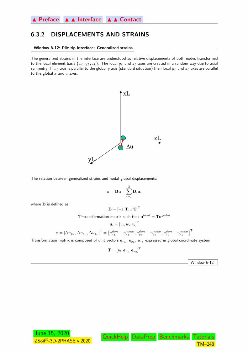
N Preface N N Interface N N Contact
6.3.2 DISPLACEMENTS AND STRAINS
Window 6-12: Pile tip interface: Generalized strains
The generalized strains in the interface are understood as relative displacements of both nodes transformedto the local element basis xL, yL, zL. The local yL and zL axes are created in a random way due to axialsymmetry. If xL axis is parallel to the global y axis (standard situation) then local yL and zL axes are parallelto the global x and z axes.
t
n1
n2
masterslave
1
2
3
4
Δu
2ΔuxL
yL
zL
The relation between generalized strains and nodal global displacements:
ε = Bu =
2∑i=1
Biui
where B is defined as:B = [−1 T, 1 T]
T
T–transformation matrix such that ulocal = Tuglobal
ui = [ui, wi, vi]T
ε = [∆uxL,∆uyL ,∆uzL ]
T=[uslavexL− umaster
xL, uslaveyL − umaster
yL , uslavezL − umaster
zL
]TTransformation matrix is composed of unit vectors exL
, eyL , ezL expressed in global coordinate system
T = [et, en1 , en2 ]T
Window 6-12
June 15, 2020ZSoilr-3D-2PHASE v.2020
QuickHelp DataPrep Benchmarks TutorialsTM–248
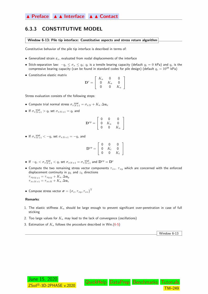
N Preface N N Interface N N Contact
6.3.3 CONSTITUTIVE MODEL
Window 6-13: Pile tip interface: Constitutive aspects and stress return algorithm
Constitutive behavior of the pile tip interface is described in terms of:
• Generalized strain εx, evaluated from nodal displacements of the interface
• Stick-separation law: −qc ≤ σx ≤ qt; qt is a tensile bearing capacity (default qt = 0 kPa) and qc is thecompressive bearing capacity (can be found in standard codes for pile design) (default qc = 1038 kPa)
• Constitutive elastic matrix
De =
Kn 0 00 Kn 00 0 Kn
Stress evaluation consists of the following steps:
• Compute trial normal stress σxtrialN+1 = σxN +Kn ∆ux
• If σxtrialN+1 > qt set σxN+1 = qt and
Dep =
0 0 00 Kn 00 0 Kn
• If σx
trialN+1 < −qc set σxN+1 = −qc and
Dep =
0 0 00 Kt 00 0 Kt
• If −qc < σx
trialN+1 < qt set σxN+1 = σx
trialN+1 and Dep = De
• Compute the two remaining stress vector components τxz, τxy which are concerned with the enforceddisplacement continuity in yL and zL directionsτxyN+1 = τxyN +Kn ∆uyτxzN+1 = τxzN +Kn ∆uz
• Compose stress vector σ = σx, τxy, τxzT
Remarks:
1. The elastic stiffness Kn should be large enough to prevent significant over-penetration in case of fullsticking
2. Too large values for Kn may lead to the lack of convergence (oscillations)
3. Estimation of Kn follows the procedure described in Win.(6-5)
Window 6-13
June 15, 2020ZSoilr-3D-2PHASE v.2020
QuickHelp DataPrep Benchmarks TutorialsTM–249

N Preface N N Interface N N Contact
6.3.4 STIFFNESS MATRIX AND ELEMENT FORCE VECTOR
Ke = π rpile2BTDB
fe = π rpile2BTσ
Remarks:
1. rpile is a radius of pile
June 15, 2020ZSoilr-3D-2PHASE v.2020
QuickHelp DataPrep Benchmarks TutorialsTM–250

N Preface N N Interface
6.4 NAIL INTERFACE
This interface is fully compatible with the interface designed for 3D piles. However, there exist the threemajor differences among them. The first is such that the nail interface can be used both for 2D and 3Dproblems, the radius appearing in the integration of the internal force vector and interface stiffness matrix isequal to the radius of the injection zone, and contact constitutive model is purely adhesive. Hence, firictionalterms in the formulation are cancelled. The detailed explanations are given in sections devoted to pilestreated as beam elements embedded in the continuum 6.2.
June 15, 2020ZSoilr-3D-2PHASE v.2020
QuickHelp DataPrep Benchmarks TutorialsTM–251

N Preface N N Interface
6.5 FIXED ANCHOR INTERFACE
This interface is fully compatible with the interface designed for 3D piles. However, there exist the threemajor differences among them. The first is such that the fixed anchor interface can be used both for 2Dand 3D problems, the radius appearing in the integration of the internal force vector and interface stiffnessmatrix is equal to the radius of the injection zone and contact constitutive model is purely adhesive. Hence,firictional terms in the formulation are canceled. The detailed explanations are given in sections devoted topiles treated as beam elements embedded in the continuum 6.2.
June 15, 2020ZSoilr-3D-2PHASE v.2020
QuickHelp DataPrep Benchmarks TutorialsTM–252

N Preface
Chapter 7
GEOTECHNICAL ASPECTS
TWOPHASE MEDIUM
EFFECTIVE STRESSES
SOIL PLASTICITY
INITIAL STATE
SOIL RHEOLOGY
ALGORITHMIC STRATEGIES
June 15, 2020ZSoilr-3D-2PHASE v.2020
QuickHelp DataPrep Benchmarks TutorialsTM–253
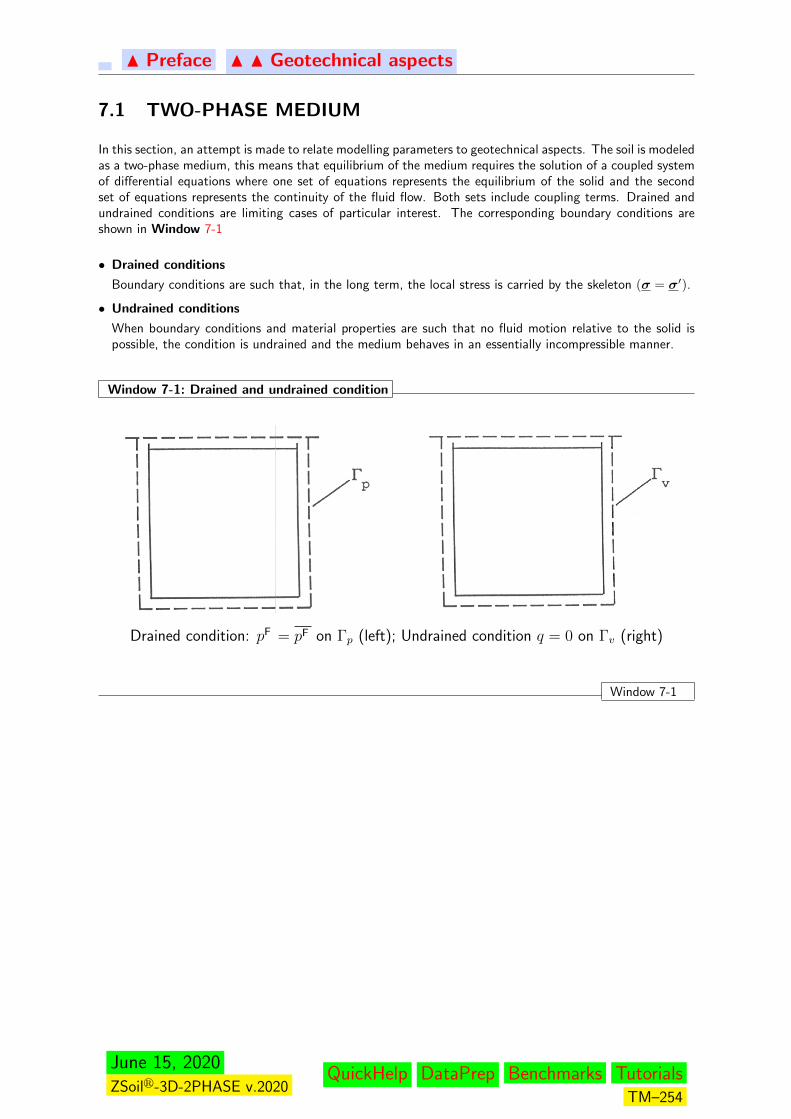
N Preface N N Geotechnical aspects
7.1 TWO-PHASE MEDIUM
In this section, an attempt is made to relate modelling parameters to geotechnical aspects. The soil is modeledas a two-phase medium, this means that equilibrium of the medium requires the solution of a coupled systemof differential equations where one set of equations represents the equilibrium of the solid and the secondset of equations represents the continuity of the fluid flow. Both sets include coupling terms. Drained andundrained conditions are limiting cases of particular interest. The corresponding boundary conditions areshown in Window 7-1
• Drained conditions
Boundary conditions are such that, in the long term, the local stress is carried by the skeleton (σ = σ′).
• Undrained conditions
When boundary conditions and material properties are such that no fluid motion relative to the solid ispossible, the condition is undrained and the medium behaves in an essentially incompressible manner.
Window 7-1: Drained and undrained condition
Drained condition: pF = pF on Γp (left); Undrained condition q = 0 on Γv (right)
Window 7-1
June 15, 2020ZSoilr-3D-2PHASE v.2020
QuickHelp DataPrep Benchmarks TutorialsTM–254

N Preface N N Geotechnical aspects
7.2 EFFECTIVE STRESSES
Effective stresses allow a unified approach to the analysis of the drained and undrained conditions, thisconcept is extended here to account for partially saturated media. Let:
σ = σ′ + pF S δ
where σ′ is the effective (grain to grain stress) , pF the interstitial pressure, and S the saturation ratio.
June 15, 2020ZSoilr-3D-2PHASE v.2020
QuickHelp DataPrep Benchmarks TutorialsTM–255

N Preface N N Geotechnical aspects
7.3 SOIL PLASTICITY
DRUCKER-PRAGER VERSUS MOHR-COULOMB CRITERION
CAP MODEL
DILATANCY
June 15, 2020ZSoilr-3D-2PHASE v.2020
QuickHelp DataPrep Benchmarks TutorialsTM–256

N Preface N N Geotechnical aspects N N N Soil plasticity
7.3.1 DRUCKER-PRAGER VERSUS MOHR-COULOMB CRITE-RION
It is common to describe soils as elastic–perfectly plastic Mohr–Coulomb materials. A smooth Mohr–Coulombcriterion described earlier is available in this program. If a Drucker–Prager criterion with cap closure ispreferred, the size of the Drucker–Prager criterion can be adjusted to match the Mohr–Coulomb criterion.This is illustrated in Window 7-2. The various matching options are derived in the theoretical section; forplane strain, the most meaningful matching for an ultimate load analysis is the matching of collapse loads.The most important size–adjustments are summarized in Window 7-2.
Window 7-2: Matching Mohr-Coulomb and Drucker-Prager criteria
Deviatoric sections of Mohr–Coulomb (M–C) and Drucker–Prager
Matching aφ k
External apices2 sinφ√
3(3− sinφ)
6c cosφ√3(3− sinφ)
Internal apices2 sinφ√
3(3 + sinφ)
6c sinφ√3(3 + sinφ)
Plane–strain collapsesinφ
3D; D =
(aψ sinφ+
√1− 3a2
ψ
)c cosφD−1
Elastic domainsinφ
3c cosφ
(plane strain νt = 0.5)1
aφ, k : parameters of the Drucker–Prager criterionφ : friction angleC : cohesionψ : angle of non–associativity (in doubt, use default value)
Window 7-2
Related Topics
• THEORY: M-C VERSUS D-P
June 15, 2020ZSoilr-3D-2PHASE v.2020
QuickHelp DataPrep Benchmarks TutorialsTM–257

N Preface N N Geotechnical aspects N N N Soil plasticity
7.3.2 CAP MODEL
The cap model accounts for nonlinear behavior of soil under dominant volumetric (pressure) stress. Theinitial size of the cap is derived from the oedometric test, it is determined by the preconsolidation pressure.Once the yield point (i.e. the cap) is reached by the stress, hardening takes place.
Hardening results from the reduction of the void ratio under increasing pressure, it is again controlled by theoedometric test.
Related Topics
• CAP MODEL
• CAP MODEL - STRESS POINT ALGORITHM
• OEDOMETRIC TEST
June 15, 2020ZSoilr-3D-2PHASE v.2020
QuickHelp DataPrep Benchmarks TutorialsTM–258

N Preface N N Geotechnical aspects N N N Soil plasticity
7.3.3 DILATANCY
Two alternative dilatancy parameters can be accommodated by the material models proposed earlier. Thefirst parameter, d, relies on the availability of experimental results. The second one, ψ , assumes the empiricalknowledge of ψ, by analogy with the friction angle φ.
• Dilatancy parameter d
Volumes changes in soils, in the plastic regime, are conveniently described as follows; let d be the dilatancy
d =dεpVdεpD
=∂Q/∂p
∂Q/∂q=rprq
where dεpV is the volumetric plastic strain increment and dεpD is the plastic deviatoric strain increment.Q is the plastic potential, rp is the norm of the volumetric plastic flow component and rq, the deviatoricone. dεpV , dεpD will usually be retrieved from a tri-axial test and rp/rq will be derived from the plasticmodel.
• Dilatancy extraction from triaxial test
Experimental results from a triaxial test can be plotted as follows:
εV = ε1 + 2ε3
εD = (2/3)(ε1 − ε3)
In the plastic regime dεV ∼= dεPV and dε ∼= dεP hence:dεVdεD
= d
• Dilatancy with Drucker-Prager plasticity
The plastic potential is in this case:Q = aψI1 +
√J2
then,
rp =∂Q
∂p=∂Q
∂I1
∂I1∂p
= 3aψ
rq =∂Q
∂q=
∂Q
∂√J2
∂√J2
∂p= 1/
√3
and finally,
d = 3√
3aψ
Given d from the experiment, aψ can be found for the material model.
• Dilatancy with Mohr-Coulomb plasticity
Plastic flow is again governed by a Drucker-Prager type surface in the program, even when yield is governedby a Mohr-Coulomb criterion. The rate of non-associativity generated by a given (experimental) d istherefore dependent on the size adjustment.
In 2D, for size adjustment option ”matching plane strain collapse load” , given φ, c and d, one gets:
June 15, 2020ZSoilr-3D-2PHASE v.2020
QuickHelp DataPrep Benchmarks TutorialsTM–259
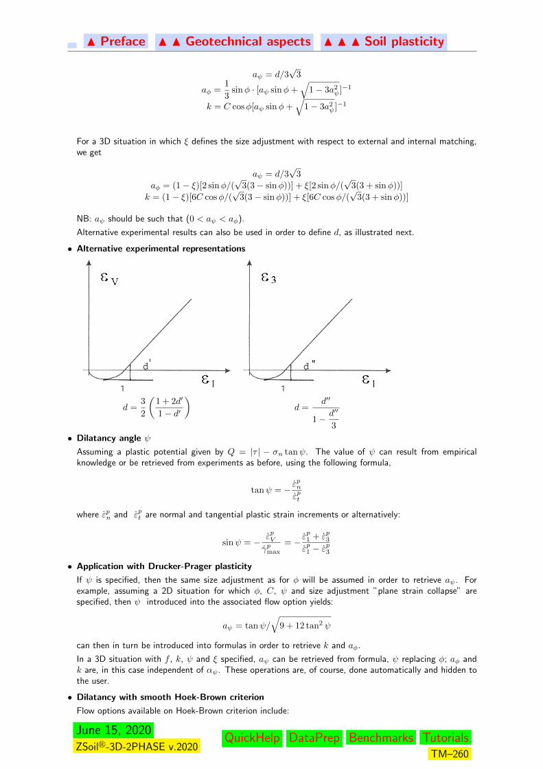
N Preface N N Geotechnical aspects N N N Soil plasticity
aψ = d/3√
3
aφ =1
3sinφ · [aψ sinφ+
√1− 3a2
ψ]−1
k = C cosφ[aψ sinφ+√
1− 3a2ψ]−1
For a 3D situation in which ξ defines the size adjustment with respect to external and internal matching,we get
aψ = d/3√
3
aφ = (1− ξ)[2 sinφ/(√
3(3− sinφ))] + ξ[2 sinφ/(√
3(3 + sinφ))]
k = (1− ξ)[6C cosφ/(√
3(3− sinφ))] + ξ[6C cosφ/(√
3(3 + sinφ))]
NB: aψ should be such that (0 < aψ < aφ).
Alternative experimental results can also be used in order to define d, as illustrated next.
• Alternative experimental representations
d =3
2
(1 + 2d′
1− d′
)d =
d′′
1− d′′
3
• Dilatancy angle ψ
Assuming a plastic potential given by Q = |τ | − σn tanψ. The value of ψ can result from empiricalknowledge or be retrieved from experiments as before, using the following formula,
tanψ = − εpn
εpt
where εpn and εpt are normal and tangential plastic strain increments or alternatively:
sinψ = −εpVγpmax
= − εp1 + εp3εp1 − ε
p3
• Application with Drucker-Prager plasticity
If ψ is specified, then the same size adjustment as for φ will be assumed in order to retrieve aψ. Forexample, assuming a 2D situation for which φ, C, ψ and size adjustment ”plane strain collapse” arespecified, then ψ introduced into the associated flow option yields:
aψ = tanψ/
√9 + 12 tan2 ψ
can then in turn be introduced into formulas in order to retrieve k and aφ.
In a 3D situation with f , k, ψ and ξ specified, aψ can be retrieved from formula, ψ replacing φ; aφ andk are, in this case independent of αψ. These operations are, of course, done automatically and hidden tothe user.
• Dilatancy with smooth Hoek-Brown criterion
Flow options available on Hoek-Brown criterion include:
June 15, 2020ZSoilr-3D-2PHASE v.2020
QuickHelp DataPrep Benchmarks TutorialsTM–260

N Preface N N Geotechnical aspects N N N Soil plasticity
F Deviatoric, corresponding to incompressible flow.
F Tensile meridian. The flow will be radial in the deviatoric plane and follow the normal to the tensilemeridian in the meridian plane.
F ψc prescribed (Hoek-Brown flow).
ψc is defined as the angle of dilatancy at failure under uniaxial compression ψc = arctan(dξ/dρ) and[arctan(
ft√2fc
) < ψc < arctan(1√2
)
].
Alternatively ψc = arctan[1√6
dI1
d√J2
; the resulting dilatancy will vary with loading paths: from coinci-
dence with the loading path under uniaxial tension to ψc under uniaxial compression.
Following table contains indicative values of dilatancy characteristics
ψ/φ d ψc, []o
Clay 0 0 -Sand - - -
Gravel - - -Rock 0.67− 1 - -
Concrete - - 4o − 35o
June 15, 2020ZSoilr-3D-2PHASE v.2020
QuickHelp DataPrep Benchmarks TutorialsTM–261

N Preface N N Geotechnical aspects
7.4 INITIAL STATE
COEFFICIENT OF EARTH PRESSURE AT REST, K0
STATES OF PLASTIC EQUILIBRIUM
INFLUENCE OF POISSON’S RATIO
COMPUTATION OF THE INITIAL STATE
INFLUENCE OF WATER
June 15, 2020ZSoilr-3D-2PHASE v.2020
QuickHelp DataPrep Benchmarks TutorialsTM–262

N Preface N N Geotechnical aspects N N N Initial state
7.4.1 COEFFICIENT OF EARTH PRESSURE AT REST, K0
K0 is by definition the ratio of horizontal effective stresses to vertical effective stresses
K0 =σ′1σ′2.
The coefficient can be determined from triaxial experiments, measured with a pressuremeter or evaluatedusing approximate formula. Commonly used formula are given in Window 7-3.
Window 7-3: Coefficient of earth pressure at rest, K0
Normally consolidated soil (NC) (K0)NC = 1− sinφ [JAK48]Overconsolidated soil (OC) (K0)OC = (K0)NCOCRα
α = sinφConfined elastic medium K0 = ν
1−ν
Window 7-3
• Overconsolidation ratio (OCR)
The overconsolidation ratio OCR is obtained from an oedometric test. It is maximum close to soil surfaceand tends to 1 a depth. The identification of OCR is illustrated in
Window 7-4.
Given the void ratio, the water content, a preconsolidation pressure can be associated with each verticalstress and the corresponding overconsolidation ratio can be computed as illustrated in Figs 7-4, 7-4.
June 15, 2020ZSoilr-3D-2PHASE v.2020
QuickHelp DataPrep Benchmarks TutorialsTM–263

N Preface N N Geotechnical aspects N N N Initial state
Window 7-4: Overconsolidation ratio OCR
• Effective stress at depth z :σ′z = γ′z,
• initial void ratio:
e0 =
(γs
1 + w
γ
)− 1
where:γs : unit weight of solid particlesw : water content ratio
Oedometric test
Vertical stresse and preconsolidation pressure as a function of depth(right).Overconsolidation ratio as a function of stress (left)
Window 7-4
June 15, 2020ZSoilr-3D-2PHASE v.2020
QuickHelp DataPrep Benchmarks TutorialsTM–264

N Preface N N Geotechnical aspects N N N Initial state
7.4.2 STATES OF PLASTIC EQUILIBRIUM
The section deals with the case of semi-infinite soil mass with horizontal or inclined surface subjected togravity load. Coefficients of horizontal pressure K fulfilling different stress criterion are investigated.
MOHR-COULOMB CRITERION
DRUCKER-PRAGER CRITERION
June 15, 2020ZSoilr-3D-2PHASE v.2020
QuickHelp DataPrep Benchmarks TutorialsTM–265

N Geotech. asp. N N Initial ... N N N States of plastic ...
7.4.2.1 MOHR-COULOMB MATERIAL
The plastic equilibrium at depth h of a semi–infinite soil mass with horizontal surface, considered as aMohr–Coulomb material, subjected to gravity loading is characterized by two circles in a Mohr diagram(Window 7-5).
The two Mohr circles correspond to Rankine states. The small circle corresponds to the active Rankine state,the large circle to the passive state.
A cohesionless material is considered first. Note that the principal stress orientation coincides with axes 1(horizontal) and 2 (vertical). The plastic stress state at depth h is
σ2 = γh (vertical)
σ1 = σ3 (assumption)
σ1 = σA = KAγh (horizontal, active state)
σ1 = σp = KAγh (horizontal, passive state)
Stress states such that,σ1 = K0γh with KA < K0 < KP
are elastic. K0 is the earth pressure coefficient at rest.
From geometrical considerations equations 1 and 2 (Window 7-5) can be derived for KA and KP are plottedand provide a useful way to define possible horizontal stress states, given the friction angle. For an elasticperfectly plastic material, no stress state outside of these limits is tolerable.
June 15, 2020ZSoilr-3D-2PHASE v.2020
QuickHelp DataPrep Benchmarks TutorialsTM–266
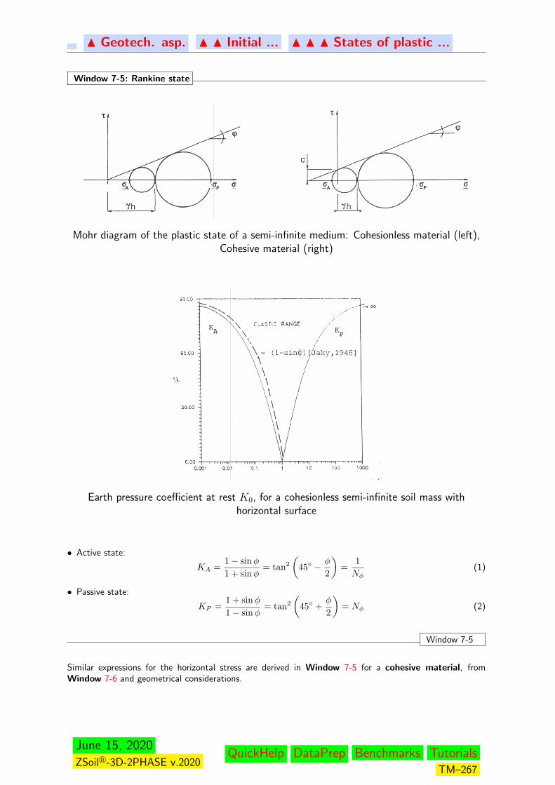
N Geotech. asp. N N Initial ... N N N States of plastic ...
Window 7-5: Rankine state
Mohr diagram of the plastic state of a semi-infinite medium: Cohesionless material (left),Cohesive material (right)
Earth pressure coefficient at rest K0, for a cohesionless semi-infinite soil mass withhorizontal surface
• Active state:
KA =1− sinφ
1 + sinφ= tan2
(45 − φ
2
)=
1
Nφ(1)
• Passive state:
KP =1 + sinφ
1− sinφ= tan2
(45 +
φ
2
)= Nφ (2)
Window 7-5
Similar expressions for the horizontal stress are derived in Window 7-5 for a cohesive material, fromWindow 7-6 and geometrical considerations.
June 15, 2020ZSoilr-3D-2PHASE v.2020
QuickHelp DataPrep Benchmarks TutorialsTM–267
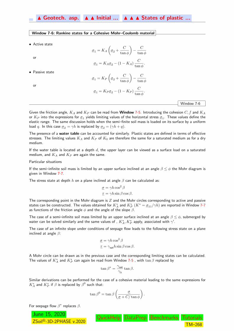
N Geotech. asp. N N Initial ... N N N States of plastic ...
Window 7-6: Rankine states for a Cohesive Mohr–Coulomb material
• Active state
σ1 = KA
(σ2 +
C
tanφ
)− C
tanφor
σ1 = KAσ2 − (1−KA)C
tanφ.
• Passive state
σ1 = KP
(σ2 +
C
tanφ
)− C
tanφor
σ1 = KPσ2 − (1−KP )C
tanφ.
Window 7-6
Given the friction angle, KA and KP can be read from Window 7-5. Introducing the cohesion C, f and KA
or KP into the expressions for σ1 yields limiting values of the horizontal stress σ1. These values define theelastic range. The same discussion holds when the semi–finite soil mass is loaded on its surface by a uniformload q. In this case σ2 = γh is replaced by σ2 = (γh+ q).
The presence of a water table can be accounted for similarly. Plastic states are defined in terms of effectivestresses. The limiting values KA and KP of K0 are therefore the same for a saturated medium as for a drymedium.
If the water table is located at a depth d, the upper layer can be viewed as a surface load on a saturatedmedium, and KA and KP are again the same.
Particular situations
If the semi–infinite soil mass is limited by an upper surface inclined at an angle β ≤ φ the Mohr diagram isgiven in Window 7-7.
The stress state at depth h on a plane inclined at angle β can be calculated as:
σ = γh cos2 β
τ = γh sinβ cosβ.
The corresponding point in the Mohr diagram is Z and the Mohr circles corresponding to active and passivestates can be constructed. The values obtained for K∗A and K∗P (K∗ = σ11/γh) are reported in Window 7-7as functions of the friction angle φ and the angle of the slope β.
The case of a semi–infinite soil mass limited by an upper surface inclined at an angle β ≤ φ, submerged bywater can be solved similarly and the same values of , K∗A,K
∗P apply, associated with γ′.
The case of an infinite slope under conditions of seepage flow leads to the following stress state on a planeinclined at angle β:
σ = γh cos2 β
τ = γsath sinβ cosβ.
A Mohr circle can be drawn as in the previous case and the corresponding limiting states can be calculated.The values of K∗A and K∗P can again be read from Window 7-5 , with tanβ replaced by
tanβ∗ =γsat
γbtanβ.
Similar derivations can be performed for the case of a cohesive material leading to the same expressions forK∗A and K∗P if β is replaced by β0 such that:
tanβ0 = tanβ
(σ
σ + C/ tanφ
).
For seepage flow β∗ replaces β.
June 15, 2020ZSoilr-3D-2PHASE v.2020
QuickHelp DataPrep Benchmarks TutorialsTM–268

N Geotech. asp. N N Initial ... N N N States of plastic ...
Window 7-7: Rankine states, inclined surface
Mohr diagram for a semi–infinite soil mass with inclined surface. Cohesionless soil
Earth pressure coefficient at rest K∗0 , for a cohesionless semi–infinite soil mass with surfaceinclined at angle β
K∗A =(
cos2 β − cosβ√
cos2 β − cos2 φ) (
cos2 φ)−1
(1− sinφ cosα) (1)
K∗P =(
cos2 β − cosβ√
cos2 β − cos2 φ) (
cos2 φ)−1
(1− sinφ cosα) (2)
with
α = arcsin
(sinβ
sinφ
)− β; β ≤ φ
α = arcsin
(sinβ
sinφ
)+ β
The horizontal stresses corresponding to active and passive states are expressed as:
• active state:
(σ11)A = K∗Aγh−C
tanφ
June 15, 2020ZSoilr-3D-2PHASE v.2020
QuickHelp DataPrep Benchmarks TutorialsTM–269
N Geotech. asp. N N Initial ... N N N States of plastic ...
• passive state:
(σ11)P = K∗P γh−C
tanφ
where K∗A and K∗P are read from Window 7-7.
Window 7-7
June 15, 2020ZSoilr-3D-2PHASE v.2020
QuickHelp DataPrep Benchmarks TutorialsTM–270

N Geotech. asp. N N Initial ... N N N States of plastic ...
7.4.2.2 DRUCKER-PRAGER MATERIAL
Rankine states can be derived similarly for a Drucker–Prager cohesionless material, with the stress statedefined previously. With the assumption σ3 = σ1 , equations (DP1) Window 7-8 are derived. With theassumption σ3 = 0.5 (σ1 + σ2), relations (DP2) result.
The results obtained for KA and KP as function of φ are reported in Window 7-8. It is observed thatthe elastic ranges of Mohr–Coulomb and Drucker–Prager materials coincide, for the assumption that σ3 =0.5 (σ1 + σ2).
As before, the presence of a surface load or of a water table can be accounted for, as for the Mohr–Coulombcase.
Window 7-8: Rankine states for Drucker-Prager material
Earth pressure coefficient at rest K0 for cohesionless material, Mohr–Coulomb (M–C),Drucker–Prager σ3 = σ1 (DP1) and Drucker-Prager with σ3 = 0.5 (σ1 + σ2) (DP2)
KA =
√3− sinφ
2 sinφ+√
3, KP =
−(√
3− sinφ)
2 sinφ−√
3(1)
KA =1− sinφ
1 + sinφ, KP =
1 + sinφ
1− sinφ(2)
Window 7-8
June 15, 2020ZSoilr-3D-2PHASE v.2020
QuickHelp DataPrep Benchmarks TutorialsTM–271
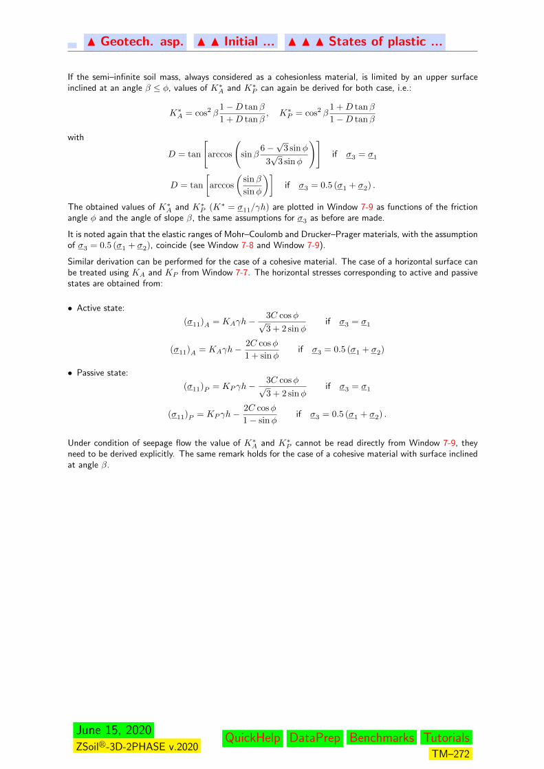
N Geotech. asp. N N Initial ... N N N States of plastic ...
If the semi–infinite soil mass, always considered as a cohesionless material, is limited by an upper surfaceinclined at an angle β ≤ φ, values of K∗A and K∗P can again be derived for both case, i.e.:
K∗A = cos2 β1−D tanβ
1 +D tanβ, K∗P = cos2 β
1 +D tanβ
1−D tanβ
with
D = tan
[arccos
(sinβ
6−√
3 sinφ
3√
3 sinφ
)]if σ3 = σ1
D = tan
[arccos
(sinβ
sinφ
)]if σ3 = 0.5 (σ1 + σ2) .
The obtained values of K∗A and K∗P (K∗ = σ11/γh) are plotted in Window 7-9 as functions of the frictionangle φ and the angle of slope β, the same assumptions for σ3 as before are made.
It is noted again that the elastic ranges of Mohr–Coulomb and Drucker–Prager materials, with the assumptionof σ3 = 0.5 (σ1 + σ2), coincide (see Window 7-8 and Window 7-9).
Similar derivation can be performed for the case of a cohesive material. The case of a horizontal surface canbe treated using KA and KP from Window 7-7. The horizontal stresses corresponding to active and passivestates are obtained from:
• Active state:
(σ11)A = KAγh−3C cosφ√3 + 2 sinφ
if σ3 = σ1
(σ11)A = KAγh−2C cosφ
1 + sinφif σ3 = 0.5 (σ1 + σ2)
• Passive state:
(σ11)P = KP γh−3C cosφ√3 + 2 sinφ
if σ3 = σ1
(σ11)P = KP γh−2C cosφ
1− sinφif σ3 = 0.5 (σ1 + σ2) .
Under condition of seepage flow the value of K∗A and K∗P cannot be read directly from Window 7-9, theyneed to be derived explicitly. The same remark holds for the case of a cohesive material with surface inclinedat angle β.
June 15, 2020ZSoilr-3D-2PHASE v.2020
QuickHelp DataPrep Benchmarks TutorialsTM–272
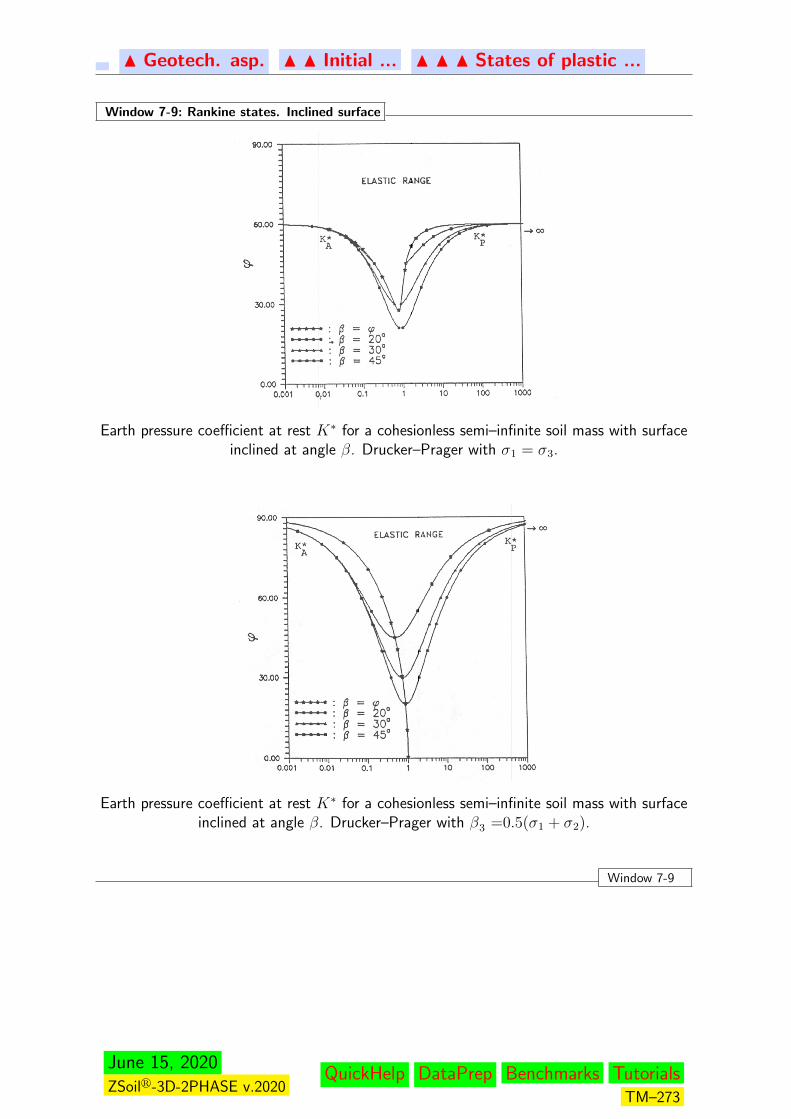
N Geotech. asp. N N Initial ... N N N States of plastic ...
Window 7-9: Rankine states. Inclined surface
Earth pressure coefficient at rest K∗ for a cohesionless semi–infinite soil mass with surfaceinclined at angle β. Drucker–Prager with σ1 = σ3.
Earth pressure coefficient at rest K∗ for a cohesionless semi–infinite soil mass with surfaceinclined at angle β. Drucker–Prager with β3 =0.5(σ1 + σ2).
Window 7-9
June 15, 2020ZSoilr-3D-2PHASE v.2020
QuickHelp DataPrep Benchmarks TutorialsTM–273
N Preface N N Geotechnical aspects N N N Initial state
7.4.3 INFLUENCE OF POISSON’S RATIO
Let Π12 be the plane containing axes 1 and 2 in which the plane strain problem is defined. If failure is tooccur in the Π12 plane, σ3 must be the intermediate stress; hence the following condition must apply:
σ1 ≤ σ3 ≤ σ2.
Simultaneously, plane strain holds, i.e. for the elastic case:
σ3 = ν (σ1 + σ2) and ν ≤ 0.5.
The following limiting conditions results:
1.
σ3 = σ1 =
(ν
1− ν
)σ2
2.σ3 = 0.5 (σ1 + σ2) .
The second one result from the limits of Poisson’s ratio. If no tectonic stresses are present, all elastic stateslies within these limits.
These conditions are sometimes met a priori by the boundary–value problem (e.g. for the box shapedmedium) or by the adopted matching of Drucker–Prager/Mohr–Coulomb criteria, as e.g. for the elasticmatching proposed earlier. Violating these conditions can have a significant effect on the solution.
In addition, some choices of material data lead to plastic behavior already under gravity loading. Since this isthe most common loading in soil mechanics, it is interesting to investigate the corresponding limits of elasticbehavior. Some situations of special interest are analyzed next for a cohesionless material.
Case 1: Box-shaped medium under gravity load, dry, matching collapse load.
The box-shaped medium is the default configuration adopted in the program. Combining plane strain andthe boundary conditions associated with the box–shaped medium leads for the isotropic medium to:
σ1 = σ3 =
(ν
1− ν
)σ2; σ2 = γh
Notice that this coincides with a limiting condition established previously for failure to occur in the plane Π12
and to the active Rankine state. This condition is therefore satisfied a priori. The invariants correspondingto this stress state are:
I1 =
(1 + ν
1− ν
)σ2 = 3σ J2 =
1
3
(1− 2ν
1− ν
)2
σ2.
In stress space, the corresponding stress point is located on a cone with its vertex at the origin, characterizedby:
aσI1 −√J2 = 0
from which,
3aσ =
√J2
σ=√
3
(1− 2ν
1 + ν
).
For a cohesionless soil, aσ characterizes the position of the stress point with respect to the yield surface.Elastic and plastic stress states can be identified as follows:
aσ < aφ : elastic stateaσ = aφ : plastic limitaσ > aφ : out–of–balance state
Using the matching rules discussed earlier with aσ replacing aφ , relations are established which define theelastic limit as a function of φ and ν.
Matching the collapse loads corresponding to Mohr–Coulomb and Drucker–Prager criteria, under plane strainconditions and deviatoric flow, yields the following result:
June 15, 2020ZSoilr-3D-2PHASE v.2020
QuickHelp DataPrep Benchmarks TutorialsTM–274
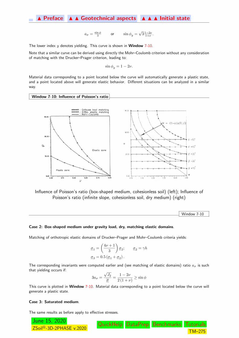
N Preface N N Geotechnical aspects N N N Initial state
aσ = sinφ3 or sinφy =
√3 1−2ν
1+ν .
The lower index y denotes yielding. This curve is shown in Window 7-10.
Note that a similar curve can be derived using directly the Mohr–Coulomb criterion without any considerationof matching with the Drucker–Prager criterion, leading to:
sinφy = 1− 2ν.
Material data corresponding to a point located below the curve will automatically generate a plastic state,and a point located above will generate elastic behavior. Different situations can be analyzed in a similarway.
Window 7-10: Influence of Poisson’s ratio
Influence of Poisson’s ratio (box-shaped medium, cohesionless soil) (left); Influence ofPoisson’s ratio (infinite slope, cohesionless soil, dry medium) (right)
Window 7-10
Case 2: Box-shaped medium under gravity load, dry, matching elastic domains.
Matching of orthotropic elastic domains of Drucker–Prager and Mohr–Coulomb criteria yields:
σ1 =
(4ν + 1
3
)σ2; σ2 = γh
σ3 = 0.5 (σ1 + σ2) .
The corresponding invariants were computed earlier and (see matching of elastic domains) ratio aσ is suchthat yielding occurs if:
3aσ =
√J2
σ=
1− 2ν
2 (1 + ν)≥ sinφ
This curve is plotted in Window 7-10. Material data corresponding to a point located below the curve willgenerate a plastic state.
Case 3: Saturated medium.
The same results as before apply to effective stresses.
June 15, 2020ZSoilr-3D-2PHASE v.2020
QuickHelp DataPrep Benchmarks TutorialsTM–275
N Preface N N Geotechnical aspects N N N Initial state
Case 4: Infinite slope at angle β, dry, matching collapse loads.
Principal stresses are:σ1 = γh(1− sinβ)
σ2 = γh(1 + sinβ)
σ3 = γ(σ1 + σ2) = 2νγh
Corresponding invariants are:I1 = 2 (1 + ν) γh
J2 =1
3(γh)
2 (3 sin2 β + 1− 4ν + 4ν2
)then
3aσ =
√J2
σ=
√3(3 sin2 β + (1− 2ν2)
)2 (1 + ν)
.
Note that, for failure to occur in plane Π12, σ3 must be the intermediate stress. This yields:
ν ≥ 1− sinβ
2(see Window 7-10 ) .
Similarly, the adjustment of yield criteria for place strain collapse load yields:
3aσ =
√3(3 sin2 β + (1− 2ν2)
)2 (1 + ν)
> sinφ.
For each given slope β in a cohesionless soil, a curve φ = f(ν) can be drawn, which characterizes the limitof elastic behavior and, for the given boundary-value-problem, the limit of stability (Window 7-5).
Case 5: Infinite slope at angle β, dry medium, matching elastic domains (Window 7-10).
Adjustment of yield criteria for coincidence of elastic domains, with νt = 0.5. The state of principal stressesis:
σ1 = γh(1− sinβ)
σ2 = γh(1 + sinβ)
σ3 = 0.5(σ1 + σ2) = γh
The corresponding invariants are:I1 = 3γh
J2 = γ2h2 sin2 β
with elastic matching of failure criteria, this corresponds to yield if:
sinβ > sinφ.
The stress state in a cohesionless soil, for the adopted adjustment with the Mohr–Coulomb criterion, will beelastic if β < φ and plastic if β > φ. Poisson’s ratio has no influence in this particular case.
Case 6: Infinite slope at angle β, saturated.
The same results as before apply, corresponding to effective stresses.
June 15, 2020ZSoilr-3D-2PHASE v.2020
QuickHelp DataPrep Benchmarks TutorialsTM–276
N Preface N N Geotechnical aspects N N N Initial state
7.4.4 COMPUTATION OF THE INITIAL STATE
Box-shaped medium in plane strain
For most static plane strain problems the soil half–plane can be conveniently approximated by a box–shapedmedium with smooth lateral boundaries (Window 5.4.9). The particular stress-strain state which resultscan easily be derived.
From plane strain and lateral boundary conditions :
ε3 = 0→ σ3 = ν (σ1 + σ2)
ε1 = 0→ σ1 = ν (σ2 + σ3)
therefore:σ1 =
ν
1− νσ2
The stress-strain fields which result for some typical loading cases are summarized in Window 7-11.
Gravity field
As can be seen in Window 7-11 the correct implementation of gravity requires simultaneous application ofγ and corresponding initial stresses. This combination is characterized by the capital Γ in this text.
An initial state corresponding to an urban environment can be established using the same procedure.
Axisymmetric medium
The default boundary conditions for the axisymmetric case are the same as for plane–strain.
June 15, 2020ZSoilr-3D-2PHASE v.2020
QuickHelp DataPrep Benchmarks TutorialsTM–277
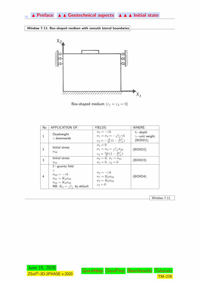
N Preface N N Geotechnical aspects N N N Initial state
Window 7-11: Box-shaped medium with smooth lateral boundaries
Box-shaped medium (ε1 = ε3 = 0)
No APPLICATION OF: YIELDS: WHERE:
1Deadweightγ downwards
σ2 = −γhσ1 = σ3 = − ν
1−ν γh
ε2 = −γhE (1− 2ν2
1−ν )
h−depthγ−unit weight(BOXD1)
2Initial stressσ02
σ2 = 0σ1 = σ3 = ν
1−νσ02
ε2 = σ02
E (1− 2ν2
1−ν )
(BOXD2)
3Initial stressσ01
σ2 = 0, σ1 = σ01
σ3 = 0, ε2 = 0(BOXD3)
4
Γ−gravity fieldγσ02 = −γhσ01 = K0σ02
σ03 = K0σ02
NB: K0 = ν1−ν by default
σ2 = −γhσ1 = K0σ02
σ3 = K0σ02
ε2 = 0
(BOXD4)
Window 7-11
June 15, 2020ZSoilr-3D-2PHASE v.2020
QuickHelp DataPrep Benchmarks TutorialsTM–278

N Preface N N Geotechnical aspects N N N Initial state
7.4.5 INFLUENCE OF WATER
A steady state Darcy flow model only is included, although the pressure b.c. can vary in time and for eachstep steady state solution can be obtained.
June 15, 2020ZSoilr-3D-2PHASE v.2020
QuickHelp DataPrep Benchmarks TutorialsTM–279

N Preface N N Geotechnical aspects
7.5 SOIL RHEOLOGY
Soil is subjected to long term deformations which cannot be avoided. This phenomenon is called consolidation.
Modern consolidation theories split the deformations into several mechanisms and two time periods associatedwith primary and secondary consolidation.
Primary consolidation is dominated by a mechanism of stress–induced seepage flow which transfers progres-sively the part of load carried by the interstitial water to the soil skeleton. During secondary consolidation,after stabilization of primary consolidation, the deformation is dominated by creep mechanisms.
Creep can be split into volumetric and deviatoric components.
A carreful choice of boundary to avoid meaningless results.
June 15, 2020ZSoilr-3D-2PHASE v.2020
QuickHelp DataPrep Benchmarks TutorialsTM–280

N Preface N N Geotechnical aspects
7.6 ALGORITHMIC STRATEGIES
SEQUENCES OF ANALYSES
EXCAVATION, CONSTRUCTION ALGORITHM
June 15, 2020ZSoilr-3D-2PHASE v.2020
QuickHelp DataPrep Benchmarks TutorialsTM–281

N Preface N N Geotech. aspects N N N Alg. strategies
7.6.1 SEQUENCES OF ANALYSES
Most combinations of drivers are possible provided they are meaningful: initial state, stability, ultimate load,prestress, consolidation, creep, flow. Obviously, an initial state analysis should come first; a stability analysisshould not be followed by any other type of analysis unless provisions are taken to restart before the stabilityanalysis; recall that the stability analysis goes through the change of the material properties.
June 15, 2020ZSoilr-3D-2PHASE v.2020
QuickHelp DataPrep Benchmarks TutorialsTM–282
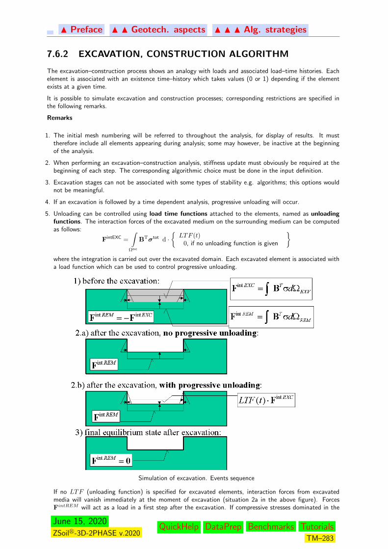
N Preface N N Geotech. aspects N N N Alg. strategies
7.6.2 EXCAVATION, CONSTRUCTION ALGORITHM
The excavation–construction process shows an analogy with loads and associated load–time histories. Eachelement is associated with an existence time–history which takes values (0 or 1) depending if the elementexists at a given time.
It is possible to simulate excavation and construction processes; corresponding restrictions are specified inthe following remarks.
Remarks
1. The initial mesh numbering will be referred to throughout the analysis, for display of results. It musttherefore include all elements appearing during analysis; some may however, be inactive at the beginningof the analysis.
2. When performing an excavation–construction analysis, stiffness update must obviously be required at thebeginning of each step. The corresponding algorithmic choice must be done in the input definition.
3. Excavation stages can not be associated with some types of stability e.g. algorithms; this options wouldnot be meaningful.
4. If an excavation is followed by a time dependent analysis, progressive unloading will occur.
5. Unloading can be controlled using load time functions attached to the elements, named as unloadingfunctions. The interaction forces of the excavated medium on the surrounding medium can be computedas follows:
FintEXC =
∫Ωexc
BTσtot d ·LTF (t)
0, if no unloading function is given
where the integration is carried out over the excavated domain. Each excavated element is associated witha load function which can be used to control progressive unloading.
Simulation of excavation. Events sequence
If no LTF (unloading function) is specified for excavated elements, interaction forces from excavatedmedia will vanish immediately at the moment of excavation (situation 2a in the above figure). ForcesFintREM will act as a load in a first step after the excavation. If compressive stresses dominated in the
June 15, 2020ZSoilr-3D-2PHASE v.2020
QuickHelp DataPrep Benchmarks TutorialsTM–283
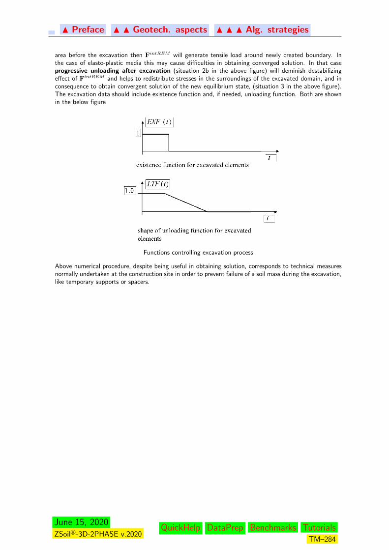
N Preface N N Geotech. aspects N N N Alg. strategies
area before the excavation then FintREM will generate tensile load around newly created boundary. Inthe case of elasto-plastic media this may cause difficulties in obtaining converged solution. In that caseprogressive unloading after excavation (situation 2b in the above figure) will deminish destabilizingeffect of FintREM and helps to redistribute stresses in the surroundings of the excavated domain, and inconsequence to obtain convergent solution of the new equilibrium state, (situation 3 in the above figure).The excavation data should include existence function and, if needed, unloading function. Both are shownin the below figure
Functions controlling excavation process
Above numerical procedure, despite being useful in obtaining solution, corresponds to technical measuresnormally undertaken at the construction site in order to prevent failure of a soil mass during the excavation,like temporary supports or spacers.
June 15, 2020ZSoilr-3D-2PHASE v.2020
QuickHelp DataPrep Benchmarks TutorialsTM–284
N Preface N N Geotech. aspects N N N Alg. strategies
Index
3Danalysis and drivers, DP: 15, 16, DP: 80
3D analysisbeams, TM: 173, TM: 178, TM: 181, TM:
183, TM: 190continuum finite elements, TM: 103, 104EAS, TM: 113elastic model, TM: 41membranes, TM: 208, TM: 211, TM: 216numerical integration, TM: 105, TM: 145shells, TM: 198trusses, TM: 157, TM: 160
Analysisbatch processing, DP: 623restart computation, DP: 622run computation, DP: 621run computation without writing *.dat, DP:
636Auxiliary planes, DP: 129Axisymmetry
analysis and drivers, DP: 15, TU: 15, DP: 16,DP: 80
beams (shells), TM: 171, TM: 178, TM: 181,TM: 183, TM: 190
continuum finite elements, TM: 103, 104EAS, TM: 113–115, TM: 117elastic model, TM: 43foot benchmark, BM: 22, BM: 24membranes, TM: 208, TM: 211, TM: 216numerical integration, TM: 105, TM: 145trusses and rings, TM: 156, TM: 160, TM:
164
Beam hingesbenchmarks, BM: 96, BM: 98, BM: 101
Beams, TU: 23, TM: 170analytical solution benchmarks, BM: 66–68,
BM: 79, 80axisymmetric shell benchmarks, BM: 83–85create/outline/update/delete elements, DP:
275create/outline/update/delete subdomain 2D,
TU: 31, DP: 164create/outline/update/delete subdomain 3D,
DP: 164hinges, TM: 188orientation 2D, TU: 31, TM: 171orientation 3D, TM: 171
reinforced concrete benchmarks, BM: 71, 72,BM: 74
Reinforcement sets, DP: 620reinforcements set, DP: 282, DP: 288subdomain 2D parameters, DP: 183subdomain 3D parameters, DP: 183
Bearing capacity, DP: 30–32foot benchmark, BM: 16
Boundary conditionsfor humidity, DP: 224, DP: 391for humidity on macro-elements, DP: 224for pore pressure, DP: 217, DP: 392for pore pressure on macro-elements, DP: 217for solid phase, DP: 379for temperature, DP: 221, DP: 386for temperature on macro-elements, DP: 221periodic, DP: 399
Consolidation, TU: 19algorithm, TM: 138analytical solution benchmarks, BM: 39geotechnical aspects, TM: 254material model, TM: 44numerical implementation, TM: 98overconsolidation ratio, TM: 263problem statement, TM: 29
Construction algorithmanalysis and drivers, DP: 16, TM: 283
Contactmacromodel, TU: 23, TU: 95, TU: 105, TU:
111Continuum 2D elements, DP: 301Continuum 2D macromodel
Automatic mesh generation, DP: 198, 199Mesh morphing, DP: 200Semi-automatic mesh generation, DP: 194,
195Subdomain generation, DP: 163, 164Virtual mesh, DP: 193–196
Continuum 3D elements, DP: 307Continuum 3D macromodel
Mesh morphing, DP: 201Semi-automatic mesh generation, DP: 196,
197Subdomain generation, DP: 165–168, DP: 170,
DP: 172, DP: 174Virtual mesh, DP: 196, 197
Convection 2D macromodelSubdomain generation, DP: 205
Convection 3D macromodel
June 15, 2020ZSoilr-3D-2PHASE v.2020
QuickHelp DataPrep Benchmarks TutorialsTM–285
N Preface N N Geotech. aspects N N N Alg. strategies
Subdomain generation, DP: 205Convection elements, DP: 366Convergence, TM: 130Creep
analytical solution benchmark, BM: 46standard properties, DP: 525swelling properties, TM: 86, DP: 525
Dynamicsadded masses, DP: 417consistent mass matrix, DP: 85control parameters, TU: 48, DP: 85Domain Reduction Method (DRM), TU: 48,
DP: 460driver, TU: 48HHT scheme, DP: 85lumped mass matrix, DP: 85mass filtering, DP: 87Newmark scheme, DP: 85Reylaigh damping, DP: 85Seismic input, DP: 618
Elasticityconstants, DP: 7material properties, DP: 518
Elasto-plastic 1Dmodel, TM: 227, DP: 594
Evolution functions, DP: 614Excavation/Stage construction
algorithm, TM: 283existence function, TM: 283show steps in preprocessor, TU: 31, TU: 95,
TU: 105, TU: 111unloading function, TM: 283unloading function benchmark, BM: 37
Existence functions, TM: 283, DP: 608
FE model preprocessingcommon methods to copy elements/nodes,
DP: 260common methods to delete elements/nodes,
DP: 260common methods to move elements/nodes,
DP: 260common methods to outline elements/nodes,
DP: 260common methods to rotate elements/nodes,
DP: 260Finite elements
selection strategy, DP: 95, DP: 97stabilization of pressure oscillations, DP: 97volumetric locking, DP: 96
Flowanalysis, DP: 15, 16, TU: 28, DP: 50, TU:
101benchmarks, BM: 57fluid head boundary condition, TU: 28, TU:
101flux boundary condition, DP: 51, DP: 227
initial conditions, DP: 51initial state driver, DP: 50, DP: 53, TU: 101material data, TU: 28, TM: 44–46, DP: 50,
TU: 101, DP: 521pressure boundary condition, TU: 28, DP: 51,
DP: 217steady state driver, TU: 28, DP: 50, DP: 54time dependent drivers, DP: 54transient driver, DP: 50, DP: 55
Fluxes on elementsfluid, DP: 425heat, DP: 428humidity, DP: 429
Fluxes on macromodelfluid, DP: 227heat, DP: 230humidity, DP: 233
Gravity, DP: 616body load components, DP: 616direction, DP: 616
Heatanalysis, DP: 15, 16, TU: 38, DP: 56analytical solution benchmark, BM: 61flux boundary conditions, TM: 36, DP: 57,
DP: 230initial conditions, TM: 36, TU: 38, DP: 57,
58initial state driver, TU: 38, DP: 56, DP: 58material properties, TM: 36, TU: 38, DP: 532numerical implementation, TM: 100problem statement, TM: 36steady state driver, DP: 56, DP: 59temperature boundary conditions, TM: 36,
DP: 57, DP: 221thermal strains, TU: 38, DP: 81time dependent drivers, DP: 56, DP: 59transient driver, TU: 38, DP: 56, DP: 60
Hingesin beam elements, TM: 217, DP: 281, DP:
597in shell elements, TM: 219, DP: 375, DP: 600
Humidityanalysis, DP: 15, 16, DP: 61flux boundary conditions, TM: 38, DP: 62,
DP: 233humidity boundary conditions, TM: 38, DP:
62, DP: 224hygral strains, DP: 61, DP: 81initial conditions, TM: 38, DP: 62, 63initial state driver, DP: 61, DP: 63material properties, TM: 38, DP: 61, DP: 534problem statement, TM: 38steady state driver, DP: 64time dependent drivers, DP: 61, DP: 64transient driver, DP: 65
Infinite elements, TM: 120, DP: 334
June 15, 2020ZSoilr-3D-2PHASE v.2020
QuickHelp DataPrep Benchmarks TutorialsTM–286
N Preface N N Geotech. aspects N N N Alg. strategies
analytical solution benchmarks, BM: 52Initial condition
for displacements, DP: 454for humidity, DP: 438, DP: 441for pore pressure, DP: 431for solid velocities, DP: 454for temperature, DP: 435
Initial statealgorithm, TM: 133earth pressure at rest (Ko), TM: 263, TM:
265geotechnical aspects, TM: 262
Initial state Komaterial properties, DP: 529
Interface 2DMaterial data groups, TM: 230, TM: 241,
TM: 246, TM: 251, 252Material models, TM: 230, TM: 241, TM:
246, TM: 251, 252Interface 2D macromodel
Subdomain generation, DP: 211Interface 3D
Material data groups, TM: 230, TM: 241,TM: 246, TM: 251, 252
Material models, TM: 230, TM: 241, TM:246, TM: 251, 252
Interface 3D macromodelSubdomain generation, DP: 211
Interface elements, TM: 230, TM: 241, TM: 246,TM: 251, 252, DP: 342
Interface elements for large deformations, DP: 356
Kinematic constraints, DP: 462
Large deformationsanalysis and drivers, DP: 16
Linear equation solvers, DP: 90skyline, DP: 90sparse, DP: 90
Load time functions, DP: 610Loads
body, DP: 404on beam elements, DP: 415on element surfaces, DP: 408on nodes, DP: 406on subdomain boundaries, DP: 248
Macromodeling2D mesh mapping, DP: 156Bore holes, DP: 471Extrusion direction, DP: 159Fluid flux, DP: 227Heat flux, DP: 230Humidity BC, DP: 224Humidity flux, DP: 233Nails, TU: 78, DP: 241Objects, DP: 146Piles, TU: 111, DP: 236Point, DP: 144
Point loads, DP: 256Pressure BC, DP: 217Subdomain, DP: 160Subdomain parameters, DP: 182Surface load, DP: 248Temperature BC, DP: 221Virtual to real mesh conversion, DP: 201
Macromodeling objectsArc, DP: 149Circle, DP: 150common methods, DP: 147Delete methods, DP: 155DXF import, DP: 154Line, DP: 148Line(s) on edge(s), DP: 150Outline methods, DP: 155Point, DP: 148Split by plane, DP: 154Surface intersection, DP: 151, DP: 202Surface on Q4 skeleton, DP: 151Surface on T3 skeleton, DP: 151Update methods, DP: 156
Main Z Soil menuAnalysis options, DP: 621Assembly options, DP: 100Control options, DP: 13, 14Control:analysis and drivers, DP: 16Extras, DP: 636File options, DP: 11Help, DP: 638Postpro, DP: 624System configuration, DP: iii, DP: 637toolbars, DP: 10
Materialscreep properties group, TM: 79, DP: 525data groups, DP: 518databases, DP: 480elastic properties group, DP: 518flow properties group, TM: 44, DP: 521handling, DP: 478heat properties group, DP: 532humidity properties group, DP: 534initial Ko properties group, DP: 529local stability properties group, DP: 535models, TM: 39, DP: 480properties varying in space, DP: 602properties varying in time, DP: 602Rayleigh damping parameters group, DP: 536unit weight properties group, DP: 519
Materials for axisymmetric shell elementslinear elastic model, DP: 493, DP: 497nonlinear (layered) model, DP: 493, DP: 497
Materials for beam elements, DP: 482fiber model, TM: 227, 228linear elastic model, TU: 23, DP: 483, DP:
487nonlinear (layered) model, DP: 483, DP: 488,
DP: 490Materials for contact elements, DP: 499
June 15, 2020ZSoilr-3D-2PHASE v.2020
QuickHelp DataPrep Benchmarks TutorialsTM–287

N Preface N N Geotech. aspects N N N Alg. strategies
frictional contact model, DP: 500Materials for continuum elements, TM: 39, DP:
517Aging concrete model, TM: 90, DP: 538Cap model, TM: 55, DP: 540Densification model, DP: 561Drucker-Prager model, TU: 15, TM: 51, DP:
546Hoek-Brown model, DP: 566Hoek-Brown model (2002 edition), TM: 77Hoek-Brown(M-W) model, TM: 66, DP: 547HS-small model, TM: 76, DP: 556Linear elastic model, TM: 40, DP: 537Modified Cam Clay model, TM: 72, DP: 543Mohr-Coulomb (M-W) model, TM: 62, DP:
549Mohr-Coulomb model, TU: 11, TU: 19, TM:
50, DP: 554Multilaminate model, TM: 68, DP: 551Plastic damage for concrete, TM: 78, TM:
91, DP: 570Rankine(M-W) model, DP: 553
Materials for continuum elements for structures,DP: 574
Materials for fixed anchor interface elementsadhesive contact model, DP: 515
Materials for fixed anchor zone interface elements,DP: 514
Materials for heat convection elementsconvection model, DP: 574
Materials for heat radiation elementsradiation model, DP: 575
Materials for humidity convection elementsconvection model, DP: 576
Materials for infinite elementsLinear elastic model, DP: 577
Materials for membrane elements, TM: 213, DP:578
Anisotropic elasto-plastic model, TM: 213,DP: 583
Fiber elasto-plastic model, TM: 213, DP: 579Isotropic elasto-plastic model, TM: 213, DP:
583Plane stress elastic model, TM: 213, DP: 582Plane stress Hoek-Brown model, TM: 213,
DP: 582Plane stress Huber-Mises model, TM: 213,
DP: 582Plane stress Rankine model, TM: 213, DP:
582Materials for nail interface elements, TU: 78, DP:
511adhesive contact model, DP: 512
Materials for pile interface elements, TU: 111, DP:504
frictional contact model, DP: 505, DP: 509Materials for pile tip interface elements, TU: 111,
DP: 508Materials for seepage elements, DP: 585
Materials for shell elements, TM: 198, DP: 587Aging concrete model, TM: 198Fiber model, TM: 198Linear elastic model, DP: 589Nonlinear (layered) model, TM: 198, DP: 589–
591Orthotropic elastic model, DP: 593, 594
Membrane 2DThickness, TM: 215
Membrane 2D macromodelSubdomain generation, DP: 164
Membrane 3D macromodelSubdomain generation, TU: 105, DP: 180
Membranes, TU: 105, TM: 208, DP: 328reinforced soil benchmark, BM: 93
Mesh tying, DP: 467
Nodal link, DP: 464Node, DP: 268Nonlinear solvers, DP: 83
Overlaid meshesgeneration, DP: 138
Plane strainanalysis and drivers, DP: 15, 16, DP: 80beams, TM: 171, TM: 178, TM: 181, TM:
183, TM: 189box-shaped medium benchmarks, BM: 9continuum finite elements, TM: 103, 104EAS, TM: 113, TM: 117elastic model, TM: 42foot benchmark, BM: 17membranes, TM: 208, TM: 211, TM: 216numerical integration, TM: 105, TM: 145trusses, TM: 156, TM: 160
Postprocessingenvelopes for structural elements, DP: 630how do I...., DP: 626using macros, DP: 628
Preferences, DP: 143Preprocessing
FE model, DP: 102, DP: 259Macromodelling, DP: 102, DP: 143Main menu, DP: 103User interface, DP: 102
Preprocessorconstruction lines, DP: 127copy by rotation selected objects, DP: 124copy by symmetry, DP: 124copy by translation selected objects, DP: 123grid, DP: 128import geometrical model, DP: 107move selected objects, DP: 122rotate selected objects, DP: 123selection of finite elements, DP: 119selection of nodes, DP: 120show distance, DP: 136show node coordinates, DP: 136
June 15, 2020ZSoilr-3D-2PHASE v.2020
QuickHelp DataPrep Benchmarks TutorialsTM–288
N Preface N N Geotech. aspects N N N Alg. strategies
show vector, DP: 136show volume of continuum element, DP: 136snap options, DP: 128
Preprocessor menuAssembly, DP: 110Draw, DP: 125Edges/Faces selection, DP: 114Edit, DP: 121Files, DP: 106Frequently used tools, DP: 138Global selection tools, DP: 117Mesh, DP: 133Overlaid meshes, DP: 136Parameters, DP: 124Settings, DP: 141Show construction/excavation steps, DP: 140Tools, DP: 135Undo, DP: 111View, DP: 112Windows, DP: 107
Preprocessor toolbars2D mesh refinement, DP: 1343D mesh refinement, DP: 135edges selection, DP: 116faces selection, DP: 115
Problem statement, TM: 27heat, TM: 36humidity, TM: 38single phase, TM: 28two phase, TM: 29
Pushovercontrol parameters, DP: 87results, DP: 625
Pushover control node, DP: 469
Restartcontrol, DP: 83
Resultscontent, DP: 98for beam elements, DP: 99, TM: 189for continuum elements, DP: 99for shell/membrane elements, DP: 99, TM:
207nodal solid accelerations, DP: 100nodal solid velocities, DP: 100residuals at nodes, DP: 100standard nodal results, DP: 100storage frequency, DP: 83
Seepage 2D macromodelSubdomain generation, DP: 202
Seepage 3D macromodelSubdomain generation, TU: 101, DP: 202
Seepage elements, DP: 360Shell 1L
Thickness, TU: 95, TU: 111, TM: 194Shell 1L macromodel
Extrusion, TU: 95, TU: 111Subdomain generation, DP: 176–179
Virtual mesh, TU: 95, TU: 111, DP: 197Shell elements, TM: 191, DP: 314
benchmarks, BM: 87–91Shell elements with one layer of nodes, TU: 95,
TU: 111, DP: 321Shell hinges
benchmarks, BM: 107, BM: 110, BM: 113Single phase
analysis, DP: 15, 16, DP: 21driven load driver, TU: 15, DP: 28effective stress analysis, DP: 21initial state driver, DP: 24numerical implementation, TM: 97problem statement, TM: 28stability driver, TU: 11, TU: 105time dependent drivers, DP: 28total stress analysis, DP: 21, DP: 27, DP: 36
Stability, TU: 11, DP: 33algorithm, TM: 135analysis, DP: 35, 36driver, TU: 11, DP: 33–36local material setting, DP: 34, DP: 535slope benchmark, BM: 25
Strainsimposed, DP: 449, DP: 457thermal, DP: 56
Stresssign convention, DP: 3
Structuresbeams, TM: 171direction on surface, TM: 225local base, TM: 226membranes, TM: 216offset, TM: 223shells, TM: 191trusses, TM: 155
SubdomainExcavation front, DP: 185Project subdomain on surface, DP: 202
Swellinganalytical solution benchmarks, BM: 47material properties, TM: 86, DP: 525
Tendonsin continuum/shells, DP: 339
Truss 2D macromodelSubdomain generation, DP: 164
Truss 3D macromodelSubdomain generation, DP: 164
Truss elements, TM: 156, DP: 291prestress benchmark, BM: 35
Two phaseanalysis, DP: 15, 16, DP: 37box-shaped medium benchmarks, BM: 11, BM:
13consolidation driver, DP: 44driven load+steady state flow driver, DP: 42driven load+transient flow driver, DP: 43foot benchmark, BM: 23
June 15, 2020ZSoilr-3D-2PHASE v.2020
QuickHelp DataPrep Benchmarks TutorialsTM–289
N Preface N N Geotech. aspects N N N Alg. strategies
initial state driver, DP: 40numerical implementation, TM: 98problem statement, TM: 29slope stability benchmark, BM: 33stability driver, DP: 46, 47time dependent drivers, DP: 42undrained driver, BM: 19, DP: 20, DP: 22,
TM: 33, DP: 37, 38, DP: 67, DP: 522,523
Unit weightdefinitions, DP: 6in single phase problems, DP: 21, DP: 27in two phase problems, DP: 47material properties, DP: 519
Units, DP: 91basic, DP: 7, DP: 93compound, DP: 94conversion, DP: 92setting basic units, DP: 91
Viscous damper 2D macromodelSubdomain generation, DP: 208
Viscous damper 3D macromodelSubdomain generation, DP: 208
Viscous dampers, DP: 371, DP: 586
Warnings, DP: 142
June 15, 2020ZSoilr-3D-2PHASE v.2020
QuickHelp DataPrep Benchmarks TutorialsTM–290