Working Paper Number 10 Gender Sensitivity of Well-being ...
56
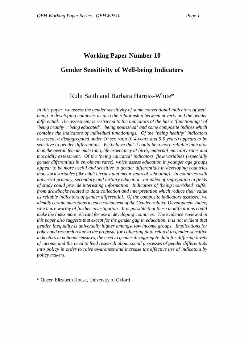
QEH Working Paper Series - QEHWPS10 Page 1 Working Paper Number 10 Gender Sensitivity of Well-being Indicators Ruhi Saith and Barbara Harriss-White* In this paper, we assess the gender sensitivity of some conventional indicators of well- being in developing countries as also the relationship between poverty and the gender differential. The assessment is restricted to the indicators of the basic ‘functionings’ of ‘being healthy’, ‘being educated’, ‘being nourished’ and some composite indices which combine the indicators of individual functionings. Of the ‘being healthy’ indicators assessed, a disaggregated under-10 sex ratio (0-4 years and 5-9 years) appears to be sensitive to gender differentials. We believe that it could be a more reliable indicator than the overall female male ratio, life expectancy at birth, maternal mortality rates and morbidity assessment. Of the ‘being educated’ indicators, flow variables (especially gender differentials in enrolment rates), which assess education in younger age groups appear to be more useful and sensitive to gender differentials in developing countries than stock variables (like adult literacy and mean years of schooling). In countries with universal primary, secondary and tertiary education, an index of segregation in fields of study could provide interesting information. Indicators of ‘being nourished’ suffer from drawbacks related to data collection and interpretation which reduce their value as reliable indicators of gender differential. Of the composite indicators assessed, we identify certain alterations to each component of the Gender-related Development Index, which are worthy of further investigation. It is possible that these modifications could make the Index more relevant for use in developing countries. The evidence reviewed in this paper also suggests that except for the gender gap in education, it is not evident that gender inequality is universally higher amongst low income groups. Implications for policy and research relate to the proposal for collecting data related to gender-sensitive indicators in national censuses, the need to gender disaggregate data for differing levels of income and the need to feed research about social processes of gender differentials into policy in order to raise awareness and increase the effective use of indicators by policy makers. * Queen Elizabeth House, University of Oxford
-
Upload
khangminh22 -
Category
Documents
-
view
1 -
download
0
Transcript of Working Paper Number 10 Gender Sensitivity of Well-being ...
QEH Working Paper Series - QEHWPS10 Page 1
Working Paper Number 10
Gender Sensitivity of Well-being Indicators
Ruhi Saith and Barbara Harriss-White*
In this paper, we assess the gender sensitivity of some conventional indicators of well-being in developing countries as also the relationship between poverty and the genderdifferential. The assessment is restricted to the indicators of the basic ‘functionings’ of‘being healthy’, ‘being educated’, ‘being nourished’ and some composite indices whichcombine the indicators of individual functionings. Of the ‘being healthy’ indicatorsassessed, a disaggregated under-10 sex ratio (0-4 years and 5-9 years) appears to besensitive to gender differentials. We believe that it could be a more reliable indicatorthan the overall female male ratio, life expectancy at birth, maternal mortality rates andmorbidity assessment. Of the ‘being educated’ indicators, flow variables (especiallygender differentials in enrolment rates), which assess education in younger age groupsappear to be more useful and sensitive to gender differentials in developing countriesthan stock variables (like adult literacy and mean years of schooling). In countries withuniversal primary, secondary and tertiary education, an index of segregation in fieldsof study could provide interesting information. Indicators of ‘being nourished’ sufferfrom drawbacks related to data collection and interpretation which reduce their valueas reliable indicators of gender differential. Of the composite indicators assessed, weidentify certain alterations to each component of the Gender-related Development Index,which are worthy of further investigation. It is possible that these modifications couldmake the Index more relevant for use in developing countries. The evidence reviewed inthis paper also suggests that except for the gender gap in education, it is not evident thatgender inequality is universally higher amongst low income groups. Implications forpolicy and research relate to the proposal for collecting data related to gender-sensitiveindicators in national censuses, the need to gender disaggregate data for differing levelsof income and the need to feed research about social processes of gender differentialsinto policy in order to raise awareness and increase the effective use of indicators bypolicy makers.
* Queen Elizabeth House, University of Oxford

QEH Working Paper Series - QEHWPS10 Page 2
Paper to be presented at the UNRISD/UNDP/CDS workshop
Gender, Poverty and Well-being: Indicators and Strategies
24-27 November 1997 Trivandrum, Kerala, India

QEH Working Paper Series - QEHWPS10 Page 3
1. INTRODUCTION
2. REMIT
3. ASSESSMENT OF WELL-BEING
3.1 APPROACHES TO WELL-BEING ASSESSMENT
3.2 PROPERTIES OF GOOD INDICATOR
3.3 GEOGRAPHICAL REGIONS COVERED
4. BEING HEALTHY
4.1 DIFFERENTIAL MORTALITY INDICATORS
4.1.1 Age specific death rates
4.1.2 A note on maternal mortality rate
4.1.3 A note on life expectancy
4.2 DIFFERENTIAL MORBIDITY INDICATORS
4.3 THE IMPACT OF POVERTY
4.3.1 Impact on mortality
4.3.2 Impact on morbidity
4.4 SUMMARY
5. BEING EDUCATED
5.1 INDICATORS OF ACCES
5.1.1 Stock variables
5.1.2 Flow variable
5.2 INDICATORS OF CONTENT AND PURPOSES
5.3 IMPACT OF POVERTY
5.4 SUMMARY
6. BEING NOURISHED
6.1 INDICATORS OF INTAKE
6.2 INDICATORS OF OUTCOME
6.3 IMPACT OF POVERTY
6.4 SUMMARY

QEH Working Paper Series - QEHWPS10 Page 4
7. COMPOSITE ASSESSMENT
7.1 THE HUMAN AND GENDER-RELATED DEVELOPMENT INDEX
7.2 THE GENDER EMPOWERMENT MEASURE
7.3 IMPACT OF POVERTY
8. CONCLUDING REMARKS
8.1 IMPLICATIONS FOR POLICY AND FOR RESEARCH
9. ACKNOWLEDGEMENTS
10. REFERENCES

QEH Working Paper Series - QEHWPS10 Page 5
Gender Sensitivity of Conventional Well-Being Indicators
1. Introduction
The Fourth World Conference on Women built upon the anti-poverty momentum of the
World Summit for Social Development. High on the agenda is a fight against poverty
based not only on economic growth but also the achievement of social goals - including
gender equity. If such commitments are to be translated into effective and enabling
policies for women however, a number of analytical and research gaps need to be
addressed. In this paper we attempt to make a contribution in this direction by examining
the sensitivity of some indicators of gender inequality in well-being.
The paper is organised as follows. First the remit is clarified (Section 2). Next, we
describe the ‘functionings’ framework within which well-being will be assessed (Section
3). Indicators which relate to the basic ‘functionings’ of being healthy, being nourished,
being educated and some composite indicators which assess a combination of
functionings will be critically analysed with respect to their sensitivity to gender
inequality (Section 4 − Section 7). The paper concludes with implications for policy and
suggestions for future work (Section 8).
2. Remit
The UNRISD remit for this paper is as follows:
“...critically assess the usefulness and relevance of a selected number
of quality of life indicators - mortality, morbidity and nutritional status
- in capturing gender discrimination...[with emphasis on] ...those
indicators that are being widely used by policy making institutions to
monitor female poverty and /or gender differences in well-being”.
(Gender, Poverty and Well-Being Project Proposal)
In addressing this, it is important to distinguish two issues. The first is the identification
of gender inequality in well-being and the second the causes underlying the inequality.
This paper is only concerned with the first. Further, it will only consider differentials in
well-being as assessed by conventional quality of life indicators. The relationship
between poverty and gender differentials in these conventional indicators will also be

QEH Working Paper Series - QEHWPS10 Page 6
Traditionally, the analysis of well-being has used market purchase data to reflect1
happiness/desire fulfilment. This confuses the state of a person with the extent of his/herpossessions (Sen, 1985).
explored. The less familiar territory of indicators of autonomy and power will be covered
by a complementary paper.
3. Assessment of well-being
Male and female well-being could be assessed on the basis of commodities they possess,
of what they succeed in doing with the commodities (functionings) or of the utility
(happiness or desire fulfilment) that these give the person. The first part of this section
describes briefly the different approaches to well-being assessment. The advantages of
the functionings-based approach used in this paper, over others, particularly with
reference to assessing gender differentials are discussed (Section 3.1). Some properties
of ‘good’ indicators used to assess functionings are outlined in Section 3.2. This is
followed by a clarification of the geographical regions for which such indicators will be
analysed in this paper (Section 3.3).
3.1 Approaches to well-being assessment
Two main approaches to assessing well-being have either been utility-based (assessing
happiness or desire fulfilment) or commodities-based (assessing opulence criteria like
income, assets, and wages) . The limitations of both these in assessing well-being have1
been described extensively in the literature (for example, in Sen 1985), and are only
illustrated here. A utility-based approach which assesses well-being on the basis of
happiness achieved or desire fulfilment suffers from the drawbacks of ‘physical
condition neglect’ and ‘valuation neglect’. ‘Physical condition neglect’ is particularly
important in the context of assessing class, caste and gender differentials. For example,
a woman who is suppressed or poor and undernourished with no hope of getting a better
deal may just resign herself to this state, be happy with small comforts and desire only
what seems ‘realistic’. Judged by the metric of happiness or desire fulfilment therefore,
she may appear to be doing well although physically quite deprived. This neglect of the
physical condition is reinforced by ‘valuation neglect’. The reflective activity of
valuation, for example whether the woman would value the removal of the deprivation,
is neglected (Sen, 1985).

QEH Working Paper Series - QEHWPS10 Page 7
Similarly in the case of the commodities approach, which commonly assesses well-being
on the basis of possession of the commodities, possession may not necessarily translate
into well-being. Besides, most commodity measurements (income, consumption data,
etc.) are made on the household rather than on the individual. Assumptions are made
about the patterns of intra-household distribution. In the context of gender differentials
however, gender relations in the household may affect the intra-household distribution
such that the assumption of equal distribution does not hold.
Given the inadequacy of the above approaches, especially in the context of the
assessment of gender differential, we use the functionings approach pioneered by Sen.
This is based on an alternative notion of well-being directly concerned with a person’s
quality of life and measured on the individual through a range of social indicators (Sen
1985). The central focus of this approach is not the possession of the commodity but
what the person succeeds in doing with the commodity and its characteristics. For
example the possession of food is not as important as the outcome, or functioning, of
`being nourished’. It is beyond the scope of this paper to give the details of this approach
the reader is directed to Sen (1985) for the details and mathematical framework and
directed for critical appraisals to Dasgupta (1993) and Granaglia (1996) amongst others.
Here we simply present a list of the relevant terms along with their non-technical
meanings:
1. Commodity vector. This is the list of commodities possessed by a person. For
example, a person may have the commodity vector: [sack of rice, bicycle].
2. Commodity characteristic vector. This is the list of ‘characteristics’ of the
commodities possessed by the person. Thus, for the commodity vector above:
[nutrition, transport].
3. Functioning. A functioning is what a person succeeds in doing with a single
commodity and its characteristics, in his possession. It is an achievement of the
person. Thus for the commodity (sack of rice) with its characteristic (nutrition), the
person could achieve the functioning: (moderately nourished).
4. Functioning vector. This is a list of functionings. It gives a snapshot of a person’s
‘state of being’, given their utilisation of their commodity characteristic vector. For
example, a utilisation of the vector in 2 above, could result in: [moderately-nourished,
mobile]. Note that a functioning as in 3 above results from the use of a single

QEH Working Paper Series - QEHWPS10 Page 8
The person may have access to several alternate commodity vectors from which one will have to2
be chosen and may also be able to choose between a number of different utilisations. Forsimplicity, we are restricting access to just one commodity vector and two possible utilisations.
commodity and its characteristics. Other utilisations (for example, choosing not to use
the bicycle) could result in different functioning vectors like: [well-nourished, non-
mobile]. Each functioning vector gives the ‘state of being’.
5. Capability set. This is the set of all possible functioning vectors that a person can
achieve. This is governed by the person’s access to commodity vectors and
utilisations feasible. For example, if the person in our running example only had
access to the commodity vector shown, and was only able to choose between the
utilisations mentioned earlier, the capability set is : 2
{ [moderately-nourished, mobile], [well-nourished, non-mobile]}.
The capability set is thus obtained from applying all feasible utilisations to all possible
choices of commodity characteristic vectors. The person can then select a preferred
functioning vector from this set to lead his/her life. This is thus the person’s ‘chosen
state of being’. Thus, “just as the so-called ‘budget set’ in the commodity space
represents a person’s freedom to buy commodity bundles, the ‘capability set’ in the
functioning space reflects the person’s freedom to choose from possible livings” (Sen
1992, p 40).
6. Well-being. This is a person’s evaluation of a functioning vector, reflecting the value
placed on that ‘state of being’. Depending on the evaluation of well-being for each
functioning vector, the person will choose one of the vectors. He or she thus has a
particular level of well-being in this ‘chosen state of being’. Since the process of
evaluation varies from person to person, it would appear to confound any
straightforward comparisons of well-being. Nevertheless, as pointed out by Sen
(1985), it may be possible to agree on some minimal constraints on the different states
of well-being. This is particularly the case when dealing with basic functionings. For
example, all personal evaluations might agree that the well-being of a person with a
functioning vector [ill-nourished, mobile] will be less than one with the vector [well-
nourished, non-mobile]. A personal evaluation may be ‘partial’ in the sense that it
cannot distinguish the ordering between some vectors, for example [well-nourished,

QEH Working Paper Series - QEHWPS10 Page 9
Theoretically, the functionings approach allows well-being to be assessed by examining the3
complete capability set. This is because the extent of the freedom to choose determined by thecapability set may itself contribute to some extent to well-being. In practice, we are restricted bythe fact that data is only available for the functionings actually achieved. By further restricting ourstudy to the basic functionings listed, the space of functionings resembles the space of basic needsused by Streeten et al (1981).
non-mobile] and [moderately-nourished, mobile]. This ‘partial’ nature also extends
to the minimal constraints that are agreed upon by a group.
Sen (1985) gives examples of functionings ranging from ‘elementary’ ones like being
adequately nourished, being healthy, avoiding escapable morbidity etc. to ‘more
complex’ ones like having self-respect, taking part in the life of the community etc. In
this paper, we examine three subjectively identified functionings, namely: being healthy,
being nourished and being educated. We adopt the position that in developing countries,
gender-differentials may persist even at the level of such ‘basic’ functionings , and3
proceed to analyse indicators that can reliably capture gender-differentials in these
functionings.
The translation of gender differences in the basic functionings, to corresponding
differences in well-being makes certain assumptions. First, that the functionings
considered are so elementary as to be necessary for well-being. That is, they will appear
in the functioning vectors of all people. Second, that all personal evaluations will agree
that a differential in any one of the functionings will result in a differential in well-being.
Table 1 shows the consequences of this second assumption.
Table 1 Gender differentials in well-being
Situation ‘Being healthy’ ‘Being educated’ `Being nourished’ ‘Well-being’
(1)
Female < Male Female < Male Female < Male Female < Male
(2) (3) (4) (5)
1 No No No No
2 No No Yes Yes
3 No Yes No Yes
4 No Yes Yes Yes
5 Yes No No Yes
6 Yes No Yes Yes
7 Yes Yes No Yes
8 Yes Yes Yes Yes
At this point, it would appear that more could be said than just a “Yes” or “No” in
Column 5. For example, a simple counting of the functionings showing a differential,

QEH Working Paper Series - QEHWPS10 Page 10
appears to suggest that female well-being is worse in Situation 8 than in Situations 4, 6,
and 7. These in turn are worse than Situations 2, 3, and 5, with Situation 1 being ideal.
Note this elaboration makes the assumption that all evaluations will agree on this
ordering as well. Even finer-grained distinctions may be possible by accounting for the
extent of differentials in functioning (and not just the existence of a differential), as
captured by the values of the indicators involved. This is done by the composite
assessment indices discussed in Section 7.
We note in passing that it has not escaped our attention that a complete assessment of
well-being would account for other functionings like human agency, power, autonomy
etc. (this point is cogently argued by Razavi, 1996). By including `being educated’, we
have moved one step beyond the conventional physiology-based functionings. The
evaluation is however still restricted here to basic functionings and is in no way
complete.
0.1 Properties of good indicators
We consider a good indicator to have the following properties. It should be easily
measurable, affordable and reliable in identifying gender differentials. The reliability of
an indicator can be judged by examining the types of errors it commits. An indicator
which performs errors of commission, (i.e. identifying a differential when it does not
exist) is preferred to one that performs errors of omission (i.e. failing to capture
differential when it does exist).
0.2 Geographical regions covered
The discussion does not concentrate on any particular region in the developing world.
Studies from different parts as well as different levels of aggregation (micro-level studies
as well as international country comparisons) are drawn upon where needed to illustrate
or clarify a point. Driven by data-availability, most research on health and nutrition
concentrates on South Asia. Some studies in sub-Saharan Africa are referred to in
relation to nutrition. The discussion on education is largely confined to the global level.
Since gender gaps in education are greatest in sub-Saharan Africa and South Asia
however, some micro-level studies in these regions are drawn upon. The composite
indicators recently proposed in the Human Development Reports have not been used at
the micro -level extensively and their discussion is restricted to the global level.

QEH Working Paper Series - QEHWPS10 Page 11
Internationally comparable indicators of well-being are quite slow to be created. Meantime, rapid4
economic and social change may be accompanied by swift alterations in the relative status of thegenders. Such alterations may be highly specific (exemplified by the rising incidence of bothfemale infanticide and excess female child mortality in South India where the status of women wasformerly relatively high). In such cases the indicators and evidence are likely to be highly specificand idiosyncratic and the research participatory and activist. The United Nations, while unable todo more than act as an observer in such an arena, can at the least be seen to give legitimacy tosuch actions. Gender gaps in the physiology based functionings assessed by indicators of mortality and5
nutritional status are taken to reflect discrimination in underlying health care, treatment andnutrition. This discrimination may find explanation in the perceived worth of women theorised forIndia in economic forms by Bardhan (1974); Miller (1981); amongst others and /or in kinshipsystems theorised in cultural forms by Dyson and Moore (1983) and Dasgupta (1987a).
Razavi (1996) has argued that high differentials in mortality could co-exist without any genderdifferentials in food intake and could be largely due to differentials in the disease context andparental health behaviour.
A shortcoming in all sections is that the Latin American region has not been covered in
any detail. A further drawback is the exclusion of studies covering indicators which are
highly specific to particular situations. Rather we concentrate on internationally
comparable indicators .4
1. Being healthy
The spectrum of health ranges from good health at one extreme to morbidity somewhere
in between to the state of fatal ill-health i.e. mortality. Gender differentials in health (as
assessed by indicators of mortality and morbidity) are taken to reflect underlying
differences in care, treatment and nutrition . Indicators of mortality are considered first5
in Section 4.1 followed by a discussion of indicators of morbidity in Section 4.2. An
outline of the indicators to be discussed in the two groups is given in Figure 1. Section
4.3 looks at the relationship between poverty and gender differentials in mortality as well
as morbidity. Section 4.4 summarises the discussion on the functioning ‘being healthy’.
Figure 1 Indicators of 'being healthy'
1.1 Differential mortality indicators
Biological factors seem to ensure higher female survival than male, right from the foetal
stage and infancy onwards. During infancy females have a higher resistance to infectious
disease. Later in life, differences in sex hormones causing increased death rates in men
by accidents and other violent causes and protection in women to ischaemic heart
diseases, combine to ensure that female survival is higher than male given similar care

QEH Working Paper Series - QEHWPS10 Page 12
There is some debate on the extent to which the female advantage in survival is culturally linked. 6
Biological differences could be reinforced by social influences fostering risky behaviour in males,and until recently higher tendency of men to smoke than women (Sen, 1995). There is some impact of male migrant workers in the case of Saudi Arabia (Sen, 1995).7
(Waldron, 1983) . These differences in mortality are reflected in the female male ratio6
(FMR). The ratio is low at birth with an average of 5% more males born than females
(probably to compensate for subsequent higher male mortality). Due to higher male than
female mortality in infancy and adolescence, the FMR becomes equal by the age of 30
(Holden, 1987). Female survival continues to be higher than male in later years causing
the FMR to tip towards females. Countries in Europe and North America have on an
average 105 and sub-Saharan Africa has 102 females for every 100 males. There are
however fewer females than males in a number of Asian, Middle Eastern and North
African countries like Egypt and Iran with 97, Turkey with 95, China with 94, India with
93, Pakistan with 92 and Saudi Arabia with 84 females per 100 men (Sen, 1995). Errors
of enumeration, migration and the sex ratio at birth fail to explain these FMRs . Increased7
female mortality (over that of males) seems to be the only reasonable explanation. Since
women are hardier than men and given similar care survive better at all ages right from
the intra-uterine period, an explanation for the increased mortality is sought in social
factors. The FMR can thus be seen as an indicator which gives a summary of gender
inequality as it operates over a long time (Sen, 1995). From the view of policy
formulation and identification of points of intervention however it may be more useful
to identify the age groups responsible for the masculinisation of the FMR. Such
information is best obtained by looking at indicators of age-specific death rates which are
discussed in Section 4.1.1. A high maternal mortality rate which also contributes to
masculinisation of FMR is discussed separately in a note in Section 4.1.2. Life
expectancy which is often used as an indicator of differential mortality is discussed in a
note in Section 4.1.3.
1.1.1 Age specific death rates
Age-specific death rates are normally calculated for groups of 5 years. The age groups
which have a high impact on sex ratios are 0-4 and 5-9 and 15-34 (largely the impact of
maternal deaths). Maternal mortality rates are discussed separately in Section 4.1.2. The
under 10 mortality rates are discussed here.

QEH Working Paper Series - QEHWPS10 Page 13
The general consensus in literature appears to be that the neonatal mortality is primarily8
affected by endogenous factors which affect the foetus intra-uterine and continue to influence itssurvival for the first 4 weeks of life. Post-neonatal however is mainly determined by exogenousfactors relating to the physical environment for example, infections, respiratory or parasiticdiseases (Visaria, 1988; Waldron 1983; Caldwell and Caldwell, 1990 cited in Agnihotri, 1997). Since females have higher immunity to infections during infancy, a female post-neonatal mortalitywhich is higher than that of males could be due to behavioural discrimination.
The under-10 age group is singled out for attention for two reasons. First, in developing
countries like India, the age group with the most pronounced female disadvantage and
therefore highest mortality differentials is the juvenile i.e. under 10 years group
(Chatterjee, 1990; Bennet 1991 cited in Agnihotri, 1997). Second, under 10’s constitute
a large proportion of the total population under high mortality conditions. Differentials
in mortality in these ages therefore have a greater impact in influencing the sex ratio than
those in older age groups.
In the under 10 age group, the largest proportion of deaths occur in developing countries
in the first year of life. The infant mortality rate (IMR) is therefore distinguished from
overall juvenile mortality rates and each is discussed below in turn.
Infant mortality rate . Biologically, female infants are more robust with a higher
resistance to infections and would therefore be expected to show an infant mortality rate
lower than that of males- the average ratio of female to male infant mortality in
developed countries is 0.8 (United Nations, 1995). If females show infant mortality
higher than that of male infants, it can be inferred to be due to environmental
disadvantages related to diet and health care (Waldron, 1983).
The IMR could however give a misleading picture because the factors affecting mortality
differ between the neo-natal and post-neonatal period . Two divergent demographic8
trends could be concealed in the period labelled “infancy”. For example, a study by
Padmanabha (1982) showed a higher male mortality (19.5 per 1000 compared to 16.8 per
1000 for girls) among new-born infants (0-24 days). Post-neonatal mortality rates were
higher for females (11.9 per 1000 compared to 9.9 per 1000 for boys). The overall infant
mortality rates (29.4 per 1000 for boys and 28.7 per 1000 for girls) however obscured
these differences (Padmanabha, 1982 cited in Seddon, 1997). In such situations juvenile
(under 10) mortality rates are more transparent and sensitive to gender inequality.
Juvenile mortality rates. Disaggregated data on juvenile mortality may not be easily
available. Enumerations of male and female populations from which the female male

QEH Working Paper Series - QEHWPS10 Page 14
The juvenile sex ratio has the added benefit of eliminating the effects of sex-selective migration.9
Juvenile refers to under 10 and child refers to under 5 years of age.10
Strictly, a 0-2 and 3-9 Juvenile sex ratio would actually give sharper difference, but since the11
1981 census data available to Agnihotri only gave 5 year age group data at the district level, these0-4 and 5-9 groupings were used.
ratio (FMR) can easily be obtained are however readily obtained. In place of juvenile
mortality rates therefore, Agnihotri (1997) proposes an alternative measure which would
largely capture similar information - i.e. the under 10 FMR, also called the juvenile sex
ratio .9
Harriss, (1993) supports a further disaggregation of the juvenile sex ratio and the use of
the 1-4 ratio (i.e. FMR14) because it summarises the experience of neonatal, infant and
early childhood mortality . Chen’s (1982) research in Matlab Thana in Bangladesh, in10
the 70’s shows that by the 4th year female deaths exceeded male by 53% then fell, but
were always higher than male, peaking again during reproductive years. FMR up to age
4 therefore captures the high differentials. Agnihotri (1997) however argues that the
under 4FMR (FMR04) is not as powerful and sensitive an indicator of gender inequality
as is the FMR59. For a start FMR04 captures the excess male infant mortality, which is
essentially a biological phenomenon (Waldron,1983; and Klasen 1994 cited in Agnihotri,
1997). FMR59 on the other hand reflects the deaths occurring in the 1-4 age group in
which more females die invariably due to behavioural factors (Waldron, 1983; Miller
1981; Johansson, 1991; Kishor 1993; cited in Agnihotri, 1997). Further, since 90% of
juvenile deaths occur in the under 5 group, Agnihotri contends that FMR59 is virtually
unaffected by deaths in 5-9 age group. A combination of FMR04 and FMR59 is
therefore proposed for identifying mortality differentials in childhood as well as
identifying the age group at which differentials set in (Agnihotri, 1997) . Such11
disaggregation of the juvenile group is important because differing combinations of
FMR04 and FMR59 can give rise to apparently similar juvenile sex ratio’s thus masking
differentials in particular age groups. For example, consider groups or regions that show
a moderate to high FMR04 and a subsequent sharp drop to low FMR59 (indicative of a
female child mortality that is higher than the male - confirmed by examining mortality
data). The overall juvenile sex ratio in this case could appear balanced hiding the adverse
survival conditions for the girl child.
In the absence of discrimination, the FMR04 would be expected to be above that at birth
(i.e. above 960 for India according to the 1981 census figures) due to higher male infant
QEH Working Paper Series - QEHWPS10 Page 15
Agnihotri (1997) assigns 4 different levels to the FMRs: low (below 910), moderate (910 to 960),12
high (960 to 1000) and very high (above 1000). The cut-off value of 960 was chosen as it was closeto the FMR at birth. Other values were chosen by examining the spatial distribution of FMRswhich revealed contiguous district clusters with these FMRs as cut-off points.
In state level averages, districts within the state, which have a high FMR are able to compensate13
for ‘rogue’ districts with low FMR’s (Agnihotri, 1997). Using districts as the unit of analysisprevents such ‘masking’.
Normally the FMR59 would not be expected to be higher than the FMR04 as a pattern of excess14
female mortality that sets in early is unlikely to be reversed in later years. Agnihotri (1997)suggests that such cases, if stray, could be indicative of data errors. If persistent, he suggests thatdetailed micro-level study is advisable. Some however (for example Pisani and Zaba, 1997 cited inAgnihotri, 1997) argue that mortality rates for female children come down in the wake of pre-natalsex selection.
With an increase in infant mortality, male infant mortality would be expected to increase more15
compared to that of females since males are more vulnerable.
mortality . Assuming that the care of the child was not gendered and since males do not12
suffer any additional biological disadvantage in childhood, FMR59 would be expected
to continue to remain the same as the FMR04. Contradictions to such expected FMR04
and FMR59 values however, can shed light on the issue of gender differential mortality.
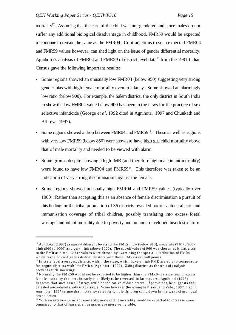
Agnihotri’s analysis of FMR04 and FMR59 of district level data from the 1981 Indian13
Census gave the following important results:
• Some regions showed an unusually low FMR04 (below 950) suggesting very strong
gender bias with high female mortality even in infancy. Some showed an alarmingly
low ratio (below 900). For example, the Salem district, the only district in South India
to show the low FMR04 value below 900 has been in the news for the practice of sex
selective infanticide (George et al, 1992 cited in Agnihotri, 1997 and Chunkath and
Athreya, 1997).
• Some regions showed a drop between FMR04 and FMR59 . These as well as regions14
with very low FMR59 (below 850) were shown to have high girl child mortality above
that of male mortality and needed to be viewed with alarm.
• Some groups despite showing a high IMR (and therefore high male infant mortality)
were found to have low FMR04 and FMR59 . This therefore was taken to be an15
indication of very strong discrimination against the female.
• Some regions showed unusually high FMR04 and FMR59 values (typically over
1000). Rather than accepting this as an absence of female discrimination a pursuit of
this finding for the tribal population of 36 districts revealed poorer antenatal care and
immunisation coverage of tribal children, possibly translating into excess foetal
wastage and infant mortality due to poverty and an underdeveloped health structure.

QEH Working Paper Series - QEHWPS10 Page 16
Agnihotri draws attention to another important distinction i.e. the decline in FMR through the16
reduction in IMR and the decline in FMR through the increase in female mortality rates in excessof male rates. The former being desirable, unlike the latter.
The high IMR with the accompanying high male IMR could result in unusually high
FMR04 and FMR59 values. Such values should therefore be investigated for excess
male mortality during infancy and under 5.
These findings led Agnihiotri to emphasise the distinction between high FMRs and
balanced FMRs. This is particularly important since, “...currently both the academic
and the policy mind set treats higher FMRs as necessarily better and reduction in
FMRs as necessarily undesirable. It is time that a distinction is made between high
FMRs and balanced FMRs. This analysis suggests a range of 960 to 980 (for India)
as a balanced figure or ‘norm’. Districts with FMRs below this level have to catch up
with the ‘norm’, districts with FMRs above this need closer scrutiny” (Agnihotri 1997,
pp140-141) . Similarly, a very high FMR at birth needs to be investigated for an 16
unsatisfactory health delivery system - as it indicates high male mortality in utero due
to poor maternal health and care.
The above results suggest that FMR04 and FMR59 are reliable indicators of a gender
differential in the functioning ‘being healthy’. Data are available from certain censuses
(such as the Indian ones) and are economically affordable and relatively easily
measurable, compared for example, to indicators of ‘being nourished’. Agnihotri’s
analysis was carried out using data which were available for the FMR04 and FMR59
groups It is possible however that FMR02 and FMR39 would reveal larger differentials
as they would capture more precisely the different mortality patterns in infancy and after.
It would therefore be desirable to repeat the analysis on these age groups. It is also worth
noting at this point that the objectivity of data can be eroded due to under-reporting, age-
heaping and other kinds of age distortions which may be gendered (for example the
underreporting of female deaths due to shame at the cause of death). Thus, however
robust these findings are for India it would be worthwhile to obtain a similar confirmation
from other countries.
1.1.2 A note on maternal mortality rate

QEH Working Paper Series - QEHWPS10 Page 17
The Capability Poverty Measure (CPM) constructed by the HDR team has 3 components One of17
these is the percentage of births unattended by trained health personnel. This is a reliableindicator of variables like the MMR and is considered a reflection of “access to reproductive healthservices and a concrete test of access to health services in general” (HDR, 1996, p110). MMR thushas a broader use as an indicator of health services in general rather than as a sole index of genderinequality in health services.
The differential death rate is high between the ages of 15-34 in developing countries,
largely due to maternal mortality (Chatterjee, 1990). Maternal mortality refers to deaths
that occur during pregnancy or within 42 days of delivery (or termination), per 100,000
live births. The maternal mortality rate (MMR) constitutes one of the biggest North-
South gaps. The latest Human Development Report gives the high figure of 471 for
developing countries as compared to 31 for industrial countries (HDR, 1997). Lack of
care during pregnancy and delivery as well as a long history of neglect with
undernourishment leading to stunting and poor physical growth all contribute to high
MMR. It cannot however be used as a sole indicator of gender inequality. The
prevalence of poverty and poor health care facilities with or without gender inequality
itself could be contributing factors to the high MMR . Besides, MMR is not capable of17
assessing differentials in situations where male well-being may be lower than the female.
1.1.3 A note on life expectancy
Life expectancy represents the mean length of time an individual is expected to live if
prevailing mortality conditions persist throughout the person’s life. It can be calculated
for individuals at the time of birth or in any subsequent age group. Life expectancy at
birth calculated for males and females is extensively used as a measure of gender
differentials in well-being by national governments as well as the World Bank and the
UNDP (as part of the Gender-related Development Index). It can however be a
misleading indicator. For example the higher mortality of females in India up to the age
of 35 is disguised by the estimated life expectancy at birth which is longer than that of
males (Chatterjee, 1990). The higher expectation in life is largely because of the greater
survival among older women which “more than compensates (mathematically speaking)
for the lower survival of younger females” (Chatterjee, 1990). This is well illustrated in
Table 2, taken from Karkal (1987) which shows the gain in life expectancy in India
between 1970-75 and 1976-80 by age for males and females. Column 3, row 1, shows
the higher gain for females of 3.146 years as compared to 1.966 years for males (column
2, row 1). Columns 4 and 5 however show that the gain for males is distributed more

QEH Working Paper Series - QEHWPS10 Page 18
evenly compared to that for females which took place mainly in the higher age groups.
The age group above 70 shows a significantly large share of 33.67 percent of the total
gain in life expectancy for females (column 5, last row) as compared to 25.10 percent for
males (last row, column 4). It is misleading therefore to conclude from the overall
increase in female life expectancy that there has been an improvement in female health
in younger ages, especially reproductive ages (Karkal, 1987). In fact Karkal showed that
the high rates of peri-natal mortality, the large proportion of low birth weight babies and
the poor chance of female survival for the same period, were an indication of the poor
health of women.
Table 2: Gain in life expectancy in India, between 1970-75 and 1976-80
Age Group Absolute Percentage
(1) (2) (3) (4) (5)
Male Female Male Female
Total 1.966 3.146 100.00 100.00
0 0.014 0.006 0.73 0.18
1-4 0.034 0.052 1.70 1.65
5-9 0.086 0.098 4.35 3.12
10-14 0.095 0.106 4.84 3.37
15-19 0.095 0.114 4.83 3.63
20-24 0.096 0.120 4.90 3.82
25-29 0.099 0.126 5.04 4.02
30-34 0.106 0.136 5.42 4.32
35-39 0.115 0.150 5.84 4.76
40-44 0.120 0.161 6.11 5.13
45-49 0.125 0.176 6.37 5.60
50-54 0.132 0.198 6.69 6.29
55-59 0.130 0.211 6.61 6.70
60-64 0.120 0.212 6.09 6.75
65-69 0.106 0.220 5.38 6.99
70+ 0.493 1.059 25.10 33.67Source: Karkal, 1987, Table 3; Computed from Sample Registration System Data
While overall life expectancy is useful as a measure of development, the use of male and
female life expectancy to capture gender differentials in well-being could therefore be
misleading, masking age specific differentials in mortality. This results in the
undesirable property of errors of omission.

QEH Working Paper Series - QEHWPS10 Page 19
1.2 Differential morbidity indicators
Whether there are sex differences in general morbidity, if reproductive disorders are
discounted is not yet clear (Chen et al; 1981, Koenig and D’Souza, 1986; McNeill,
1986a). Nevertheless, the prevailing working hypothesis is that social differences in
morbidity will result from the different types of work undertaken by people in the
household and gender division of productive and reproductive work. Such differences
will affect susceptibility, exposure, duration, severity and treatment (Caldwell and
Caldwell, 1987; Cohen, 1987; Pettigrew, 1987). For example, women’s nursing work
increases their exposure to infection contracted by other household members while
material and/or cultural constraints on resting may slow women’s recovery from infection
as well as from childbirth (Harriss, 1993). Gender differences in sanitation and
environmental hygiene have also been hypothesised as having an impact upon morbidity.
In rural North India the quality, source and degree of (faecal) contamination of bathing
and clothes washing water may be gender-specific, contributing to the sexual geography
of village life (Pettigrew, 1987). Similarly, it has been shown in rural Karnataka that the
male health environment differs from that of the female - the former is more out of doors
while the latter centres around the “dark, smoke filled kitchen” - in ways which suggest
that exposure to infection may be gender-specific (Caldwell and Caldwell, 1987).
Regional differences in climate could be interacting with underlying biological gender
differentials causing differential morbidity. For example, male infant/child mortality
were found to be much higher than female (1.51) in the mountainous Bardsir region in
Iran. Razavi (1996) speculates that this could be the result of the interaction between the
environmental conditions (cold winters) and the greater vulnerability of male infants to
respiratory disease due to the immaturity of their lungs.
Factors described above could also interact with underlying gender differentials in health,
care and nutrition causing differential morbidity. For example, a higher proportion of
deaths due to coughs and disorders of the respiratory system occur in the Indian states of
Gujarat, Haryana, Jammu and Kashmir, Madhya Pradesh, Rajasthan, Uttar Pradesh and
West Bengal. The proportion is lower in the Southern states of Andhra Pradesh,
Karnataka, Tamil Nadu and Kerala and in Orissa in the East. Chatterjee (1990) suggests
that there may be more to this regional pattern which could be dismissed as being caused
by climatic differences but which also corresponds to the North-South female mortality

QEH Working Paper Series - QEHWPS10 Page 20
dichotomy, than just coincidence. The susceptibility of women to cold climate could be
directly increased due to inadequate clothing when performing outdoor chores like
fetching water as well as due to underlying anaemia or malnutrition. Given the cold
climate, women’s domestic role and seclusion as a result of which women are closeted
in smoky kitchens, would make them vulnerable to respiratory disorders.
Despite evidence as described above of gender differences in morbidity arising due to
underlying differentials in health or nutrition, reliable indicators of morbidity have not
been developed for use by international agencies or governments because of a number
of problems with data. First, morbidity data - gathered through questionnaires - tend to
suffer from major biases (Sen, 1995). People’s perception of illness can vary greatly
depending on the medical care they normally receive and their medical knowledge. Sen
gives the example of Kerala, a state in India with a relatively higher level of education
and health care, versus Bihar which is very backward and towards the other end of the
spectrum. Despite (or because of!) the medical care and life expectancy in Kerala, the
rate of morbidity is much higher than the Indian average while that in Bihar is much
lower. Medical care while reducing actual morbidity at the same time sharpens
understanding and perceptions of one’s illness (Sen 1995). Further, such subjectivity has
particular implications when used to capture gender differentials. The material buttresses
of patriarchy are “translated into health beliefs and social customs” (Caldwell and
Caldwell, 1987). Women in West Bengal were reported as much more unwilling to
perceive or declare their ill-health than were men (Sen, 1985). Boys in Karnataka are
treated more frequently because they are believed to be sick more often on account of the
perceptions of their relative weakness in childhood (Caldwell and Caldwell, 1987).
Second, if the problem of subjectivity is overcome to some extent by using hospital
records on the incidence of disease, the data would tend to reflect the availability of
medical care. Sen gives the simple example of a village acquiring a hospital, More
people would then be treated, and thus more statistics would be available, giving the
impression of a rise in morbidity (Sen, 1995). The data would also reflect information
only with respect to those who have been taken to the hospital for treatment rather than
actual gender differences in morbidity. In cases from north India, a marked gender
imbalance in health expenditure and treatment has been recorded (Dasgupta, 1987b;
Pettigrew, 1987). Females also appear to be less often referred for allopathic treatment
than are males and are often treated using the other three indigenous health systems.

QEH Working Paper Series - QEHWPS10 Page 21
In India such data are available from the medical certification of deaths (urban areas) and the18
“causes of death (rural) survey” which is a lay-reporting survey, carried out annually in a randomsample of block-headquarter villages throughout India (Chatterjee, 1990).
‘Causes of death’ data may also be interrogated for gender specificity to gain information on19
differential mortality. In India one of these causes, ‘death by social cause’ appears to be aneuphemism for infanticide, a gross crime perpetuated almost always on female infants and neo-nates. These have been mapped by Chunkath and Athreya (1997) prior to activating socialawareness against such discrimination. Similarly such data has been used to draw inferencesabout bride-burning. While these are dramatic indicators, they are highly politically sensitive andfar from universally available.
Third, though no gender difference in the incidence of disease may be detected, there
could well be gender differences in the duration and intensity of treatment. (McNeill,
1986b in Tamil Nadu confirming Chen et al, 1981 and Koening and D’Souza 1986 in
Bangladesh).
Fourth, if data for morbidity is collected from ‘causes of death’ data available in hospitals
and/or primary health care centres in certain countries , its accuracy depends on the18
expertise of the recorder (Harriss, 1993), system of classification used and the concepts
of illness and death of those reporting (Harriss, 1991). Further it can only be employed
for inferences about morbidity if it is assumed that sickness follows the same gender and
age distribution as death (Harriss 1993) .19
Fifth, the sex bias in morbidity does not operate in a simple and consistent manner and
therefore could give misleading impressions. This is confirmed in an interesting analysis
of eye disease (Cohen 1987). Male infants from richer households were found to have
a higher incidence of iatrogenic loss of vision than females or males from poor
households, due to the use of harmful steroid eye cream. Similarly xerophthalmia
common in infants and pre-school children and resulting from Vitamin A deficiency
afflicts males up to 1.7 times as frequently as females. Paradoxically, food behaviour
which assigns “cultural superfood” to male weanlings during the post-neonatal period
while keeping females fully breastfed, may be the source of deprivation of Vitamin A.
1.3 The impact of poverty
This section summarises the findings of some studies investigating the impact of poverty
on gender differences in mortality (Section 4.3.1) and morbidity (Section 4.3.2).
1.3.1 Impact on mortality
QEH Working Paper Series - QEHWPS10 Page 22
Conclusions of studies investigating the relationship between poverty and gender bias in
child survival differ. Two contradictory arguments about class position, poverty and
mortality implicitly inform such studies. One is that the relative economic value of
women is highest and patrilineal control over poverty is lowest among the assetless poor,
so that, ceteris paribus, less gender bias would be expected (Harriss, 1991). Warrier’s
Purulia study would lend qualified support to this position (Warrier, 1987) as do findings
of less intense female discrimination in poorer households by Murthi et al (1995) and
Krishnaji (1987). The opposite arguments are that it is among the poor that both the
opportunity cost of health care in terms of income foregone and actual costs incurred are
relatively the greatest, that under conditions of food scarcity females are discriminated
against in order to preserve the patriline, and that it is amongst the poorest that any given
level of discrimination is most likely to translate itself into mortality. Dasgupta’s (1987b)
and Wadley and Derr’s (1987) evidence and Warrier’s (1987) Medinipur case lend
support to these hypotheses. Other studies suggest that material and cultural
determinations of mortality as an aspect of reproductive strategy may cut across class and
income (Dasgupta, 1987b; Visaria 1987). Such poverty may therefore not be a major
determinant of gender-differentials (Harriss, 1990 and Chen et al, 1981 and Dasgupta,
1987a cited in Murthi et al, 1995). The relationship between poverty and gender
differentials in mortality is therefore not clear-cut.
1.3.2 Impact on morbidity
As with mortality, the interaction between gender differentials in morbidity and poverty
is not straightforward. If the sexual geography of hygiene were common to all members
of a locality, then patterns of exposure to certain diseases would not be expected to be
related systematically to the economic status of households. Further, specific aspects of
morbidity often show counter-intuitive trends. For example, the case of eye disease given
earlier (Section 4.2).
1.4 Summary
Indicators of differential mortality and differential morbidity were assessed for their
ability to reliably enable the identification of gender differentials in the functioning
‘being healthy’. The findings are summarised as follows.

QEH Working Paper Series - QEHWPS10 Page 23
Differences in education potential of men and women have not been conclusively shown to be20
different. There are a number of questions in educational psychology about the issue of genderbias in test instruments themselves - the need to distinguish between an ‘ability’ and theperformance of the task designed to measure it. Without such a distinction, tests could simplyconfirm existing prejudices. (UNESCO, 1995).
• Mortality. Indicators are relatively easily measurable and economically affordable.
Certain country censuses provide information used to construct the indicators. The
reliability of some, for example life expectancy, is questionable as it can mask gender
differentials in specific age groups. Amongst the age-specific indicators, juvenile sex
ratios (particularly disaggregated into FMR04 and FMR59) appear to be reliable and
of greatest relevance to developing countries.
• Morbidity. Reliable indicators are difficult to construct due in turn to the inherent
unreliability of the underlying data (hospital records, questionnaires etc.).
• Poverty. Evidence on the relationship between poverty and gender differentials in
mortality is conflicting. While some suggest that there is no link, others suggest
higher differentials either in richer groups or poorer groups. The question always
requires answers which are grounded empirically. No a priori generalisations are
possible. Differentials in indicators of the functioning ‘being healthy’ do not therefore
essentially conflate with differences in opulence indicators.
2. Being educated
The assessment of gender differentials is relatively more straightforward with regard to
education than to health. Unlike mortality, the education potentials of men and women
do not differ . Further data related to education (for example enrolment rates, mean20
years of schooling) do not suffer from constraints of subjectivity like morbidity data.
Indicators for assessing male-female differentials in education can be broadly divided
into two groups - indicators of access or participation and indicators of content and
purposes (UNESCO: Third World Education Report, 1995). The first are more relevant
to developing countries where access could be unequal even at primary levels. The
second are mainly concerned with gender differences in the nature and content of
education provided. These are relevant to developing as well as developed countries.
The indicators discussed are shown in figure 2.
Figure 2 Indicators of 'being educated'

QEH Working Paper Series - QEHWPS10 Page 24
This is a point of general concern which applies to all the variables discussed in the paper.21
2.1 Indicators of access
These are concerned with access to education right from basic literacy to tertiary
education. Indicators of access are further sub-divided into stock variables (adult literacy,
mean years of schooling) and variables of flow (enrolment and drop-out rates). These are
discussed in turn below.
2.1.1 Stock variables
Stock variables give information about the older members of the population. Adult
literacy refers to persons (15 years and above) who can with understanding read and write
a short simple statement on everyday life (illiteracy refers to those in this age group that
cannot). The literacy rate of women is significantly lower than that of men in 66
countries (a third of the membership of the United Nations). According to UNESCO,
“few other indicators capture as decisively the imbalance in the status of men and women
in society as does this simple measure” (1995). These rates have however been criticised
for being self-reported and hence inaccurate. Another problem is the definition used. If
defined only with respect to a major national language(s), it can result in under-
estimation (UNESCO, cited in King and Hill, 1993).
The other stock variable mean years of schooling is the average number of years of
schooling received per person aged 25 and over. It overcomes some of the problems
associated with the literacy variable. Both variables however reflect past investment and
access to education. Recent progress could be better captured by looking at changes over
time in sex differentials in flow variables detailed in Section 5.1.2 This is particularly
important in developing countries where younger age groups constitute a larger
proportion of the population.
Before proceeding to discuss flow variables, it is important to be aware that when
assessing any of the variables, the use of indices is preferred over that of percentage
values. This is because the latter can be deceptive (UNESCO, 1994) . As an 21
illustration, see Table 3 (based on UNESCO, 1994). The table shows gender disparities
between male and female illiteracy rates for 1970 and estimated disparities for 2000, by
region. Disparities are expressed in the columns 2 and 3 as percentages and columns 4

QEH Working Paper Series - QEHWPS10 Page 25
The gross enrolment ratio for any level is the total enrolment in that level, regardless of age,22
divided by the population of the age-group which officially corresponds to that level. The netenrolment ratio only includes enrolment for the age-group corresponding to the official age groupfor that level. The distinction is important because enrolments could include large numbers ofover-age children as for example in primary schools in sub-Saharan Africa, the Arab states andSouthern Asia.
and 5 as indices. On comparing 1970 and 2000, in columns 2 and 3 gender disparities
appear to be diminishing in percentage points in most regions. The indices in columns
4 and 5 however suggest that the gender gap will actually widen in all regions except
Latin America.
Table 3: Comparison of indices and percentages to assess gender disparities in
illiteracy rates
Region female minus male illiteracy rate nos. of illiterate women per 100
(%) illiterate men (index)
(1) (2) (3) (4) (5)
1970 2000 1970 2000
Sub-Saharan Africa 9.3 20.6 129 169
Arab States 25.8 22.5 143 184
Latin America or 7.4 2.4 133 123
Caribbean
East Asia or Oceania 28.6 14.6 187 246
South Asia 27.9 25.0 151 174
Source: UNESCO, 1994 Table 2
2.1.2 Flow variables
These include enrolment and drop-out rates at the primary, secondary and tertiary levels.
Since wide gender gaps exist in access even at the primary and secondary levels, these
levels are of major concern here. Issues related to differentials in the nature and content
of education are more relevant to the tertiary level. The tertiary level will therefore be
dealt with in Section 5.2.
The female/male participation ratio (i.e. female gross enrolment ratio divided by male
gross enrolment ratio) at the primary level is a useful measure to assess the gender gap22
in countries which have not yet achieved universal primary education. In those that have,

QEH Working Paper Series - QEHWPS10 Page 26
Hyde, 1993 uses the term wastage in the context of sub-Saharan Africa. This includes grade23
repeaters i.e. children held back for poor performance as well as drop-outs i.e. children who leaveschool before completing a cycle of primary school education and do not re-enrol.
A number of reasons could be playing a role for such segregation in fields. In some cases there24
may be actual restriction of opportunities offered by the education system for access to particularfields of study. In others social convention may constrain the supply of female students. Possibly a
secondary enrolment rates can be utilised. There is some concern however that
participation rates could mask other important measures. For example if a large number
of enrolled students leave school before completing, it is important to know the
proportion of boys or girls that drop-out . In order to resolve the issue of which was23
more important (enrolment rates or drop-out rates), UNESCO (1995) used two indices,
the school life expectancy and the school survival expectancy. School life expectancy
is defined as the total number of years of schooling which the child can expect to receive
in the future, assuming that the probability of his or her being enrolled in school at any
particular future age is equal to the current enrolment ratio for that age (UNESCO, 1995).
The school survival expectancy is basically the school life expectancy for those persons
already in school. Using these two measures the UNESCO observed the following for
developing countries. First, the school life expectancies of girls were somewhat lower
than boys indicating that higher proportions of girls than of boys never got into school
at all. Seventeen of the 52 developing countries included in the analysis however showed
a slightly higher school life expectancy for girls than boys (particularly in the Latin
American/ Caribbean region). Second, countries with the gap in school life expectancies
most in favour of boys were generally those with low school life expectancies both for
boys and girls (particularly in sub-Saharan Africa). Third, countries with a very low
school life expectancy for girls showed less of a gap between the school survival
expectancies of boys and girls than in their school life expectancies. The conclusion was
that the main policy challenge in most of the poorest countries was less one of ensuring
the retention of girls once in school than of increasing access by designing ways and
means of encouraging parents to send girls to school in the first place.
2.2 Indicators of content and purposes
Differences in the fields of education girls and boys are enrolled in begin appearing at the
secondary level and become more pronounced at post-secondary and higher levels
(UNESCO, 1995). This phenomenon is common to developing as well as industrial
countries . Every country for which data are available to UNESCO, shows a female24
QEH Working Paper Series - QEHWPS10 Page 27
combination of both. Further perceptions of the compatibility of the careers based on differentsubjects with future marriage, household responsibilities and child-rearing are probablyimportant in girls’ attitudes and motivations towards different fields of study. Even in industrialcountries women retain the primary responsibility for child care and household management. Thisaffects both the kind of employment they are willing to accept and are likely to be offered. Therefore expectations and preferences concerning the nature of future employment are likely toinfluence the choice of fields girls make at the tertiary level (UNESCO, 1995). Some studiesinvestigate the question of differences in ability (whether females are better suited to particularfields and similarly in case of males). There are however a number of problems with assessmentwhich is widely open to prejudice and misunderstanding (detailed in UNESCO, 95). It is therefore
difficult to reach any firm conclusions. In any case, ability is obviously not the only factorresponsible for gender segregation (UNESCO, 1995).
Given social conventions and certain perceptions, the scope for disagreements when translating adifferential in higher education enrolment and segregation in education fields, into a differential inwell-being, could be greater than for differentials in ‘being healthy’, ‘being nourished’ or for ‘beingeducated’ at the primary or secondary level.
share of enrolment in the natural sciences, engineering and agriculture that is less than
the female share of total enrolment in all fields. The opposite tendency is apparent in the
humanities.
The UNESCO developed an index to assess the extent of such gender segregation
(statistical notes, UNESCO, 1995). This Gender Segregation Index gives the percentage
of persons who would need to change their fields of study for a ‘balanced’ distribution
of the sexes among the fields to be achieved (i.e. one where the ratio of females to males
is the same in all fields). Low percentages indicate a low degree of segregation or
gender-specific specialisation. Conversely high percentages indicate a high degree of
segregation of the sexes. Calculation of the index for Bangladesh indicated that 1% of
those enrolled in third level education would need to change the field of study. The
corresponding figure for Finland was 23%. This appears to indicate that there is less
gender segregation in higher education in the former than the latter. The figure obtained
however conceals the fact that there are proportionately fewer females in higher
education (16% of total students) in Bangladesh. The proportion of females in the
different fields are close to the overall percentage of 16. In case of Finland however,
females are (more) proportionally represented in higher education but under-represented
in certain fields for example natural sciences, engineering, and agriculture. To obtain the
full picture therefore differential tertiary enrolment rates must also be assessed together
with the Gender Segregation Index.
2.3 Impact of poverty

QEH Working Paper Series - QEHWPS10 Page 28
A number of factors underlie gender gaps in education. Khan, 1993 reviewing studies in South25
Asia identifies factors such as social and religious conservative norms, basic amenities in schools(such as lavatories), rigid time schedules, the demand for girls to take care of siblings and dohousehold and farm work. Similarly Hyde’s review of sub-Saharan Africa identifies negativeparental and community attitudes towards the Western education of girls, the desire to protectgirls, the poor quality of schools, constricted curriculum choices for girls, marriage and child-bearing which compete with school for older girls, and demand for girls to work at home and thefields (Hyde, 1993). Further the review identifies unfavourable labour market opportunities withgirls employed in trade and informal sectors and therefore requiring to learn from mothers andapprentice with older women, while boys have a higher opportunity to enter formal labour marketsafter education.
The UNESCO report looking at the relationship between National Income and education,
reached the conclusion that while gender gaps in access are low in rich countries, gender
gaps are not necessarily wide in all poor countries. The poorer countries with a GNP of
less than US$500 per caput (1992 figures) showed a range of female-male participation
ratios in the primary level of education which varied from under 50% for girls to nearly
100% for example Guinea 47%, Benin 50%, Kenya 98% and Rwanda 97%.
Since gender gaps in education are maximum in sub-Saharan Africa (a majority of
countries with lagging female enrolment rates in the primary level are in this region) and
in South Asia, we concentrate on micro-level studies in these regions. Micro-level
research reveals poverty is related with lower education in girls (Rozensweig, 1980 for
India; Ahmed and Hasan, 1984 for Bangladesh cited in Khan, 1993 and Assie, 1983 for
Cote d’Ivoire; Weis, 1981 cited in Hyde, 1993). Educational advantage conferred by
high socio-economic status was found to be even more pronounced at the university level
(studies reviewed by Hyde, 1993). The generally accepted conclusion is that family
poverty in rural and urban areas is probably the most important reason for holding girls
back from school or withdrawing them earlier, often reinforced by other factors.25
2.4 Summary
The findings of Sections 5.1−5.3 can be summarised as follows.
• Indicators. The most important indicator of gender gap in developing countries
appears to be enrolment rates. In countries where primary education is universal,
enrolment rates for secondary school could be used. For some developing countries
for example in Latin America/ Caribbean, enrolment is universal at all three levels.
It is then important to look at the gender segregation index.

QEH Working Paper Series - QEHWPS10 Page 29
Svedberg, 1991 subdivides energy expenditure into the following components: a) to maintain26
internal body functions like cardiovascular and respiratory activities i.e. the basal metabolic rate(BMR); b) to increase internal body activities during waking hours like increased muscle tone andfood digestion; c) external physical activity like manual labour; d) body’s generation of heat(thermogenesis) and e) energy that leaves the body unutilised in the urine and faeces. AlthoughBMR dominates most discussions, an additional component in children, which is quite bigcompared to others is growth.
• Poverty. Family poverty in rural and urban areas is probably the most important
reason for holding girls back from school or withdrawing them earlier.
It is worth noting here that it appears contradictory that sub-Saharan countries with their
balanced FMRs should show the widest gender gaps in education right from the primary
levels. Perhaps the same factors that are considered responsible for their getting a better
deal in nutrition and health care (reflected in balanced FMR) are responsible for their lack
of enrolment in school, i.e. the higher economic worth of girls and women due to high
participation in agriculture and rural trade. Further, when women work in the fields,
young daughters would be required to take care of siblings and other household
reproductive work.
Gender gaps in education in sub-Saharan Africa highlight the importance of not relying
on a single indicator. Equality in one dimension of human functioning (for example,
‘being healthy’ in sub-Saharan African countries as reflected by the balanced FMR) may
not necessarily be accompanied by equality in others. The issue of composite indices to
obtain an overall picture of well-being is the topic of discussion in Section 7.
3. Being nourished
Indicators used to assess the state of nutrition are commonly divided into two groups -
indicators of intake and indicators of outcome. These are discussed in Sections 6.1 and
6.2. Before this however, some basic terminology is outlined below (details in McNeill,
1985).
In order to survive and function, every human being (and animal) requires energy
(measured in calories). This is obtained from the constituents of food - namely,
carbohydrates, proteins and fats (together referred to as macronutrients) which also
perform other specific roles. The body is in energy balance when the energy input
(derived from the macronutrients) is equal to the energy expended (for maintenance of
the status quo and physical activity) . In addition to energy, adequate levels of26
micronutrients, namely vitamins and minerals (in small quantities) and fibre are required.

QEH Working Paper Series - QEHWPS10 Page 30
Deficiency of any of the vitamins or minerals causes specific diseases, for example
vitamin B deficiency causes beri beri and Vitamin C deficiency causes scurvy. Since the
quantity of micro-nutrients required is very small, a diet which supplies adequate energy
normally supplies adequate quantities of these as well (as it generally does with protein).
In developing countries, micro-nutrient deficiencies usually occur in members of the
population who have low total food intake and therefore also energy inadequacy. This
paper therefore does not discuss individual nutrient deficiencies but restricts itself to
energy inadequacy referred to here as undernutrition.
The two groups of indicators (intake and outcome) used to assess the state of nutrition
are discussed below with particular reference to their role in assessing gender
differentials.
3.1 Indicators of intake
In the dietary intake method, the calorie intake is calculated (normally by noting the
consumption of food) and compared against that required for the individual to be in
energy balance.
This is a commodity-based approach with the measurement of food consumption being
an opulence criterion, rather than functionings-based. For example two persons of
similar weight and performing similar physical activity may receive identical amounts
of food. While one may be adequately nourished however, parasitic infection may
interfere with food absorption in case of the other. Although the characteristics
(nutrition) of the commodity (food) remain the same, the differing properties of the
persons involved result in different functionings (being well-nourished and being under-
nourished). Although a dietary intake indicator does not therefore rest comfortably with
the functioning-based approach, it will be addressed briefly in order to highlight the
problems facing the issue of nutrition assessment in general.
Some problems facing the dietary intake method concern the following:
• Data collection. This method requires an estimation of daily food intake (and the
calculation of calories contained, using standardised conversion tables) which is time-
consuming, expensive and prone to error. The methods commonly used to estimate
food consumption are the following (Svedberg, 1991). First, recall (typically over 24
hours and preferably for seasonal sets of 24 hours) where people are asked how much

QEH Working Paper Series - QEHWPS10 Page 31
The issues under dispute with respect to each of these are discussed by Svedberg (1991) and are27
briefly outlined here. 1) Energy requirement for the basal metabolic rate (BMR) per kilo of bodyweight: The BMR could show inter-individual differences among individuals of the same sex,weight and age. Possible explanations are a) genotypic differences affecting the efficiency withwhich energy is metabolised; b) changes in body composition with increase in weight or evenbetween individuals of same weight for example, different ratios of fat to lean tissue - the energyexpenditure for the maintenance of fat stores being lower than for the sustenance of functions oflean tissue; and c) the controversial notion of adaptation to intake either by increasing energyefficiency or by reducing energy wasted by thermogenesis. Further under dispute is the form ofrelationship between BMR and body weight; whether BMR increases linearly with an increase inbody weight or if the relationship is quadratic (concave). 2) Body size: Different body size normscould be used. One possibility is the use of the height and body weight of an average individual inan “observed” reference population (or a fraction thereof) which has adequate nutrition. The otheris the average of an estimated range within which the weight can be changed without impairing
of different kinds of food they have consumed over that period. People however tend
to forget minor items or snacks, breast milk cannot be estimated by this method and
the poor are likely to exaggerate their food intake, in order to hide their deprivation.
The second method is measurement of changes in food stocks, and conversion of this
into ‘consumption’ flows. The disadvantage again is that only main meals consumed
at home are covered and breast milk is not accounted for. The third method is
weighing the equivalent of the food actually observed to have been consumed over a
fairly long period of a week or more. The method may also involve direct weighing
before consumption or the copying by the researcher of portions (raw or cooked) using
standardised estimates for the weights of known volumes. Errors may creep in the
conversion factors between raw and cooked ingredients, in the measurement of
portions and in the classification of ingredients (Harriss - White, 1997). Further, there
is widely alleged to be a trade-off between efforts to obtain high precision and
modification to behaviour on account of being observed (Abdullah, 1983). In all the
above methods it is necessary to ensure that the consumption has been measured on
‘normal’ (i.e. not fasting or feast days) days and over seasons (to exclude the impact
of exceptional events).
An additional disadvantage with particular reference to assessing gender differentials
is to do with the methodology (measurements are most commonly made on
households and rather rarely on individuals).
• Fixing the norm. Relating the intake to a presumed per capita requirement norm is
fraught with a host of problems. A calculation of the required energy depends on three
dimensions (i) energy requirement for the basal metabolic rate per kilo of body weight
(ii) body size and (iii) work activity. The calculation of the ‘norm’ for each of these
dimensions is in dispute.27

QEH Working Paper Series - QEHWPS10 Page 32
health. The weight at the lower end of this range could also be used. 3) Physical activity: Withregard to the physical activity of the reference individual, economic return of physical work differssubstantially depending on the land, capital etc. owned. While international organisations basethe norm on the “average” work activity, this actually differs for different people to enable them tosurvive economically and avoid undernutrition.
With reference to gender it is important to ensure that different norms are used for
males and females. WHO estimates suggest that an average male expends 36% more
energy per day than his female counterpart - due to differences in body weight (and
therefore higher maintenance energy) and also in the proportion of metabolically
active tissue per unit of body weight. Since females need less of most nutrients than
males, an assessment based on absolute amounts of food, rather than relative to the
different male/female norms, could result in errors of commission. Underestimating
the work load of women, especially those involved in hard agricultural labour and
heavy household work could result in biases in the calculation of norms. This could
result in an underestimation of any existing female disadvantage (an omission error
which is a more serious error).
• Inter-individual variability. Requirements at the individual level are difficult to
asses owing to substantial inter-individual variability. Thus nutrient requirements
based on averages for populations are abused if applied to individuals. For example
half of a normally distributed population will have a less than average calorie (or any
other nutrient) “requirement”. In fact the FAO and WHO acknowledge these
difficulties and suggest that their requirement norms not be used as cut-off points for
estimating undernutrition at the individual level, but be used for “prescriptive”
purposes only.
Indicators of intake thus appear to suffer from methodological (measurement on
households) as well as inherent (data, norms, inter-individual variations) problems. The
conclusions of studies investigating gender differentials differ depending on the
assumptions made about intra-household distribution, norms used, the cut-off points as
well as ungendered standards.
Studies assessing nutritional status using individual food intake measures done on the
same data set could reveal contradictory findings. For example Harriss-White, 1997
compares 5 studies (Ryan et al, 1984; Behrman, 1988; Behrman and Deolalikar, 1989;
Behrman and Deolalikar, 1990; Harriss, 1990). These studies were all carried out on the
same nutrition database (from the International Crops Research Institute for the Semi-

QEH Working Paper Series - QEHWPS10 Page 33
Arid Tropics - ICRISAT) which covers 200 individuals of all ages (except wholly breast
fed babies) from 240 households in 6 villages from 4 agro-climatically different regions
in the semi-arid tropics of India. Conclusions in all but Behrman’s study ran counter to
orthodoxy: the intra-household bias, if existing at all, was found to be against male
children by Ryan et al, (1984) and against males by Behrman and Deolalikar (1989),
whereas Behrman and Deolalikar (1990) reported a bias oscillating against and toward
females according to supplies. Harriss (1990) found some village-specific scarcity bias
which was significantly anti-children of whatever sex, some anti-adult male and some
anti-female of whatever age. Age bias rather than gender bias was also found by Ryan
et al., teenagers being most vulnerable.
Similarly contrasts exist in other published studies which are now dated. Consider two
studies in Bangladesh (Chen et al, 1981 and Abdullah, 1983) where the sex ratio is highly
masculine. Chen et al’s conclusion was that male intake per caput exceeded that of
females in all age groups. Abdullah (1983) however, made adjustments in male and
female energy requirements from recommended allowances for age groups over 5. The
conclusion of this study was that in ages above 5 there was no female discrimination
(beyond that accounted for by male female differences in body size, activity and
physiological differences). This contrast in results highlights the importance of ensuring
that the gendered norms are used for males and females. A review by Wheeler (1984)
similarly concluded that there was no evidence of discrimination against women in the
intra-household allocation of energy intakes (relative to energy requirements) in South
Asian populations (cited in Gillespie and McNeill, 1992).
Published studies in sub-Saharan Africa with regard to gender differences in intake are
extremely few. Schofield’s (1979) findings drawn from 11 African villages suggested
that there was no statistically significant difference between fulfilling established calorie
requirements between males and females − adult males fulfilled 101% and adult females
96% of the requirement (cited in Svedberg 1990).
3.2 Indicators of outcome
Three types of indicators are used to assess the outcome of calorie intake - biochemical,
clinical and anthropometric. The first two may not be useful at early stages of
undernutrition or when energy shortage is not accompanied by micronutrient deficiencies
or illnesses. Data is patchy and interpretation of causality is not straightforward as there
QEH Working Paper Series - QEHWPS10 Page 34
Height for age is used as a measure of stunting and if low indicates chronic growth retardation; 28
weight for height is a measure of wasting and if low is taken to be an indicator of recent or ‘acute’growth retardation; weight for age is a measure of overall nutritional status and indicates bothlong-term and current growth retardation - if low it is referred to as ‘underweight’.
may be reasons other than undernutrition for these clinical signs and symptoms and
biochemical findings. Further the number of clinical signs and symptoms is large (up to
36) involving difficulty in diagnosis. Svedberg, (1991) gives the example of a study
where two experienced, well-trained experts examining the same population for clinical
signs of malnutrition were in agreement in less than half of them as to which signs did
and did not occur. Biochemical assessments apart from being expensive and time-
consuming are largely used to detect isolated mineral and vitamin deficiencies.
Anthropometric measurements are the most commonly used of the outcome measures.
The measurements considered most relevant by nutritionists are height and weight. More
specifically, children are normally assessed using height for age, weight for height and
weight for age ratios . For adults the height and the Body Mass Index (weight for height28
square) are used. Svedberg (1991) expresses very succinctly the reasons for the
popularity of the use of anthropometric measurements: “the anthropometric approach
rests on the presumption that people’s physical appearance reflects their nutrition (and
health) status, i.e. if their body intake and expenditure balance at too low a level, this will
show in their body constitution. This means that neither energy intake nor the
expenditure has to be measured. The anthropometric approach is therefore more direct
and simple and less reliant on data collection than the dietary approach” (1991, p 191).
Despite these advantages, some difficulties are as follows:
• Fixing the norm. As with indicators of intake, here too the issue of fixing the ‘norm’
is controversial. Most national and international studies use the norms established by
the United States Centre for Health Statistics. Such norms are usually obtained from
Western populations assuming that the average child here is on his or her genetic
potential growth path and has a weight assumed to be optimal for health and various
mental and physical capabilities (Svedberg, 1991). First, it is highly controversial as
to whether these norms could apply to all populations. This issue could be avoided by
using norms derived from the local population from amongst a well-fed group. In case
gender inequality already exists in such a group however, using these norms would
result in omission errors (Harriss-White, 1997). Further if age is given wrongly such

QEH Working Paper Series - QEHWPS10 Page 35
This is a simplification. If a child reacts to nutritional stress by first reducing physical activity29
below the critical level, the child could be undernourished although anthropometric indicatorsremain normal. Svedberg, 1991 discusses in Section 10.2 p 244 whether a low anthropometricscore is a necessary and/or sufficient condition to label an individual as undernourished.
norms could give misleading results - for example, the overstatement of a girls’ age
could mean that anthropometric measures could erroneously suggest that she is
undernourished. Where women lie about the age of the daughter saying she is younger
(as is alleged to happen commonly in Asia), shortfalls could pass unnoticed.
Second, a child would be classified ‘undernourished’, if he/she fell below some cut-
off point below the mean of the reference population . Opinions vary on choosing29
the ‘cut-off’ point (Svedberg, 1991). For example with regard to height for age, cut-
off points vary from 10 per cent and two standard deviations below the median
reference height to below the fifth decile in the reference population. Using different
cut-off points, Mora (1984) showed that the share of children in a sample from
Columbia that were classified as wasted or stunted was almost twice as big depending
on the cut-off point used (cited in Svedberg, 1991). Setting the cut-off close to the
reference median would give high commission and low omission errors and vice
versa.
It is also often forgotten in interpretation that in a normal distribution, a certain
proportion of the population will be healthy at, and below the cut-off; just as a
proportion will have poor nutritional status due to obesity above the cut-off.
• Adaptation. The issue of adaptation is still unresolved. Briefly, if food intake in a
particular region/population/gender is lowered the body could adapt in a number of
ways (physiologically, behaviourally and metabolically) with costless adjustments to
body size. While there is no disagreement about the fact that such adjustments cannot
proceed indefinitely, there does not appear to be any agreement as to the level of the
crucial cut-off point below which adjustment impairs health (Svedberg, 1991).
• Multicausality . Anthropometric measurements are not just the outcome of nutrition.
They are also affected by the availability of health care, the ‘public health’
environment and the prevalence of infections. For example, infections in the first 24
months have consequences for height trajectories, in particular growth deviations,
which are now thought to be irreversible (Payne and Lipton, 1994). Height deficits
relative to standards are often interpreted as indicators of chronic disadvantage, though

QEH Working Paper Series - QEHWPS10 Page 36
they may be more accurately attributed to disadvantage in infancy (Harriss-White,
1997). In terms of assessing gender differentials, the fact that anthropometric
measurements could reflect multiple disadvantages could be seen as an asset in an
indicator. The other controversies which give rise to different results depending on
norms and cut-offs used (as discussed above) however greatly reduce their value.
Using anthropometric measures has the advantage of being measurable and not reliant
on recall or self-reporting. Measurements are made on individuals. Intra-household
differences in nutritional status of individuals, for example, between males and females
can therefore be assessed. Despite these advantages over intake measurements, outcome
measures are prohibitively expensive and require more skill than for example, census
enumeration data used to collect mortality statistics. Besides, they could be unreliable
giving rise to errors of commission or omission depending on the norms and cut-offs
used.
As with the dietary intake approach, the following studies which use anthropometric
outcome measures fail to arrive at a consensus on the issue of gender differentials.
Chen’s (1982) study in Bangladesh on children under 5, identified gender differentials
in all three anthropometric indicators (weight for age; weight for height and height for
age). 14.4% of the girls showed severe malnourishment (in the weight for age indicator)
compared with 5.1% of the boys and 59.9% of the girls were moderately malnourished
compared with 54.8% or the boys. Abdullah’s (1983) longitudinal study also in
Bangladesh on a smaller sample however gave no clear gender differentials in
anthropometric indicators for this age group. In fact, socio-economic factors were found
to be more important than gender in determining nutritional status (cited in Watson and
Harriss, 1985).
Again there is no direct relationship between sex ratios and anthropometry in National
nutrition surveys in Nepal and Sri Lanka. This was supported by Martorell, et al (1984)
who found no difference between boys and girls in the degree of growth retardation in
the Terai region of Nepal. Sri Lanka with a higher sex ratio than Nepal however, in a
national nutrition survey showed an anthropometric difference between girls and boys
under 5 in the height for age indicator in 10 of 12 districts (Perera, 1983 cited in Watson
and Harriss, 1985).

QEH Working Paper Series - QEHWPS10 Page 37
Findings in sub-Saharan Africa are similarly controversial. In a study of data on more
than 50 populations in the region, Svedberg (1991) concluded that females irrespective
of their age, were not at a disadvantage vis-a vis males in anthropometric status. Klasen
(1996) however questions this evidence and presents data showing an anti-female trend.
Controversies on the consistency of findings due to problems with norms and
interpretations are well-highlighted in the published correspondence between Klasen
(1996) and Svedberg (1996).
Our view that findings on gender differentials in nutritional status (assessed by both
approaches) are inconclusive is shared by Basu (1993). Basu’s thesis is that most
research in this area starts with the biased view that gender differences in nutritional
status must exist. She looks at primary data as well as critically reviewing existing
literature on sex differentials in childhood nutritional levels in South Asia. She suggests
that the evidence on the relatively greater nutritional deprivation of girls in South Asia
“is inconclusive at best and possibly even conclusive in a direction which suggests that,
in access to food, daughters and sons do not really stand very different chances”.
3.3 Impact of poverty
Few studies of nutritional status have investigated the gender differential by class. Three
studies in India (Levinson, 1972; Sen and Sengupta, 1983 and McNeill, 1984 cited in
Watson and Harriss, 1985) found that anthropometric differences in the two sexes were
specific to social class. Differences between the sexes disadvantageous to women were
greatest in ‘the poorer Ramdasia caste (Levinson) the poorer landless caste (Sen and
Sengupta) and the poorest socio-economic group (McNeill) than in the corresponding Jat
landowning class, the landed castes and the population as a whole. The results suggested
that the intensity of nutritional discrimination against females was greatest in the poorer
socio-economic class. In contrast to this, Ryan et al’s (1984) anthropometric research on
the ICRISAT database showed gender differences confined to the children of landless and
small-farmer households where it was boys rather than girls who were at a disadvantage.
The tribals in Andhra Pradesh studied by Gillespie (1988) showed gender bias in
anthropometric status which favoured boys below 12 months and favoured girls between
12 and 60 months. Rather than income poverty at the household level, it was the
participation in the labour force of the mother that was most closely and significantly
associated with malnutrition. The author suggests that increased income from labouring

QEH Working Paper Series - QEHWPS10 Page 38
is offset by reduced time for child-care and feeding in an agrarian regime where peak
labour and peak disease incidence coincide.
As with anthropometric indicators, the relation between low calorie intakes and income
poverty is not clear-cut. A documentation of 24 methodologically unstandardised micro-
level studies of individual nutrients intake in India and Bangladesh revealed the
following. First that nutrient intake per se is not a good indicator of gender poverty.
Second, that there did not appear to be a systematic age or gender bias (across villages
within a region, even with respect to the landless class) with unambiguous implications
for policy (Harriss, 1991). Miller (1997) in an extensive review of 14 studies (of intake
and anthropometric measurements) extending from the North-Western plains area of the
Indian subcontinent to the Himalayan region, the Eastern plains and the South however
concludes that a relationship between poverty and food allocation differentials exists, but
in a counter-intuitive direction. Female disadvantage in food allocation was found to be
more apparent in the propertied strata rather than the lower strata - particularly in the
Northern plains. As an explanation for this, she draws on the “poverty aversion”
approach which “takes into account the social fact that raising many daughters within the
North-Western plains socio-economic context, will indeed impoverish a family, while
sons will enrich a family” (Miller, 1997 p1692).
3.4 Summary
The findings in Sections 6.1−6.3 can be summarised as follows:
• Unreliable indicators. Measurements and calculations of food intake and outcome
suffer from a number of methodological and inherent problems which make it difficult
to construct reliable indicators.
• Poverty. Assessing the true impact of poverty on gender differential is confounded
by the absence of good indicators. Using the existing indicators, studies show
contradictory findings. It is not obvious that differentials in nutrition would always
conflate with differentials in opulence indicators.
4. Composite assessment
While differentials in well-being in each functioning can be assessed separately as in
Sections 4 6, we now turn to the issue of whether a composite assessment can be

QEH Working Paper Series - QEHWPS10 Page 39
Details of the calculation of the HDI can be obtained form technical Note 2 in HDR, 1997. A30
brief explanation follows here. For calculating the HDI, values for each component are firstnormalised to give an index. The general formula for the index X for each dimension i (i = 1 fori
longevity, i = 2 for education and i = 3 for income) for a country is as follows:
Xi =(actual x value – minimum x value) / (maximum x value – minimum x value). i i i i
Each indicator has the following fixed minimum and maximum values a) Life expectancy at birth25 and 85 years b) Adult literacy at 0% and 100% and the average enrolment ratio at 0% and100%. The education attainment index is given by combining the two with a weightage of 2/3 foradult literacy and 1/3 for combined enrolment. c) Real GDP per capita (PPP) at PPP$100 andPPP$6154. The maximum is actually 40,000$ but any value above the world average GDP ofPPP$5835 is discounted using a form of Atkinson’s formula (details are given in technical note 2,HDR, 1997). Thus the maximum is reduced to PPP$6154.
Having normalised the values of each indicator on a 0 - 1 scale, the value of the HDI is obtained byaveraging the indices for the 3 dimensions. Each index is given an equal weightage. Thus:
HDI = (X1 + X2 + X3)/3.
obtained by accounting for the extent in differences in each functioning. Attempts at
framing indices reflecting such composite assessments are not new. More recently
indices of human development have been developed by the Human Development Report
team (HDR) of the United Nations Development Programme. The Human Development
Index (HDI) which was reported in 1990 was followed by other indices namely, the
Gender-related Development Index (GDI) and Gender Empowerment Measure (GEM);
the Human Freedom Index, the Capability Poverty Measure and in the most recent report
(1997), the Human Poverty Index. It is conceivable that the methods used in developing
such indices could be extended to combine the indicators of health and education
described earlier. We leave this as an interesting exercise to be pursued, and concentrate
here on existing composite indices relevant to the issue of gender inequality viz. the GDI
(and its precursor HDI) and the GEM.
4.1 The Human and Gender-related Development Index
The Human Development Index (HDI) was designed to focus on three essential
dimensions of human functioning - longevity (or ‘being healthy’ ) measured using the
indicator life expectancy at birth; knowledge (or ‘being educated’) measured by the
indicators adult literacy and average primary, secondary and tertiary enrolment; and
access to resources to enable a decent living standard measured using the indicator per
capita income adjusted for purchasing power parity (PPP) . Normalised values (indices)30
for indicators are obtained and averaged to give the HDI. This is thus considered a
reflection of the combined well-being in the dimensions assessed and gives a value on
a scale between 1 (maximum development) and 0 (minimum). Of particular interest to
this paper is the Gender-related Development Index (GDI). The GDI could be considered

QEH Working Paper Series - QEHWPS10 Page 40
Details on measurement of GDI can be found in technical note 2 in HDR, 1995. Briefly, the 331
dimensions assessed in the GDI are the same as the HDI. The main difference is that the HDI isconcerned with overall achievement. The GDI however takes into account the extent of gender-inequality. Indices for the 3 dimensions are therefore calculated separately for male and femalei.e. X and X . These are then combined to give a gender-equity-sensitive indicator (GESI),f m
calculated by = (p X + p X ) where X and X = corresponding male and female indicesf f m m f m 1- 1- 1/(1- )ε ε ε
obtained by applying the Xi formula given in footnote 30 above to male and female indicator valuesseparately; p and p = corresponding male and female proportion of the population. ε can bef m
considered a measure of aversion to gender inequality, which can be altered anywhere between 0and ∞. 0 indicates that there is no aversion to gender inequality (the HDI implicitly assumes ε tobe 0; when ε = 0, an arithmetic mean of male and female achievements is obtained). If the ε = ∞,this indicates a very high aversion to gender inequality such that only the achievements of thegroup with the lower value, typically females, are considered while those of men are ignored. TheGDI however uses a ε = 2 which expresses a moderate aversion to inequality. This is an arbitrarydecision and the value can be altered depending on the degree of aversion the state decides on.
There is an additional difference between the HDI and GDI with reference to the income indicator.For the purposes of the GDI the shares of earned income for women and men are derived bycalculating their wage as a ratio to the average national wage and multiplying this ratio by theirshares of the labour force. Their shares of earned income are then divided by their populationshares. This gives the two proportional income shares. The GESI is then obtained as explainedabove by combining the female and male indices (X and X .). This value is then multiplied by thef m
average real adjusted GDP per capita of the country. This gives a measure of GDP per capita thatis now discounted for gender inequality. This is the Actual (x ) value used when calculating thei
index Xi for income as in the previous footnote. The GESI indices obtained for the longevity andknowledge are then combined with the Xi for income. The average of the 3 indices gives the GDI.
Technical note Table 2.4 in HDR, 1993 makes some suggestions for using different indicators to32
measure the 3 dimensions of the HDI for countries at different stages of development.
as a special type of HDI which takes note of inequalities between any two groups. The
two groups considered here are male and female (the same index could however be used
to assess the inequalities between groups of different castes or different ethnicity, etc.) .31
The GDI is simply the HDI which is discounted or adjusted downwards for gender
inequality.
The HDI and GDI have been designed for comparisons between countries at different
stages of development . If the GDI is to be used specifically in developing countries,32
certain adaptations may be required. Considering adaptations pertaining to each
component of the index in turn:
• Longevity: This component reflecting the functioning ‘being healthy’ is measured
by life expectancy which was selected over other suggestions like infant mortality rate
and potential lifetime (Desai, 1989 cited in HDR 93). This was because the IMR and
potential lifetime were not able to distinguish between industrial countries. However,
for our purpose of assessing well-being within developing countries an indicator
relating to mortality rates in younger age groups would have to be used. Further life
expectancy at birth has little or no value as a measure of gender differentials. As
discussed in Section 4, FMR04 and FMR59 are more appropriate indicators of the

QEH Working Paper Series - QEHWPS10 Page 41
The issue here therefore is of including income from waged work. Criticisms (for example33
Prabhu et al 1996) about inclusion of unpaid work are important. The information captured bysuch an indicator would however be different to that which the ‘earnings’ are expected to capture.
functioning (‘being healthy’) that life expectancy proposes to capture. Some way of
including the disaggregated FMR values in the index would need to be devised.
• Knowledge: This component reflecting the functioning ‘being educated’ is measured
by combining the indicators adult literacy (2/3 weight) and mean primary, secondary
and tertiary enrolment (1/3 weight). It has evolved from the first HDR in 1990 in
which only adult literacy (the percentage of literate people above 15) was used (HDR,
1990). Since the adult literacy rate was unable to distinguish between industrial
countries, mean years of schooling (average number of years of schooling received per
person aged 25 and over) was added. Since a substantial proportion of the population
in developing countries is under 18 and majority under 15, these stock variables were
unable to capture the flow of educational attainment (Smith, 1992 cited in HDR,
1993). In response to these criticisms subsequently ‘mean years of schooling’ was
replaced by ‘average primary, secondary and tertiary enrolment’. As discussed in
Section 5, this is a measure useful in developing countries as well as being sensitive
to gender differentials and thus a useful component of the GDI. The 1/3 weightage
given to the average enrolment measure however makes it subservient to the adult
literacy measure. It would be worth investigating empirically whether a reversal of
weights - such that adult literacy accounts for 1/3 and the average enrolment for 2/3,
would be more appropriate for use in developing countries.
• Income: For the purposes of the GDI the shares of earned income for women and men
are derived by calculating their wage as a ratio to the average national wage and
multiplying this ratio by their shares of the labour force. Any differential in the
income indicator therefore relies on two important differentials - the ratio of female
wages to male wages and the female to male ratio of the labour force. The income
indicator does not aim to reflect women’s access to income for consumption or other
uses, as women who earn money may not have any control over it within the
household. In other cases women who do not earn income may control what is earned
by male members of the household. Rather, the income variable is used in the GDI
because it reflects a family member’s earning power, which is an important factor in
economic recognition, independence and reward (HDR 1995) .33

QEH Working Paper Series - QEHWPS10 Page 42
Sen, proposes three ways through which a womans’ outside earnings ultimately
contribute to well-being. These are first by strengthening her bargaining position in
the household, second allowing her to have higher claims due to a higher perceived
contribution to the family’s economic position and third possibly giving her a clearer
perception of her individuality and well-being (Sen, 1990). Outside earnings also
positively influence the care that female children receive in comparison to male.
Table 4 from Sen (1990) gives comparative data for 5 major regions. The table shows
the relationship between women’s earnings, represented by female to male activity
rate ratios (activity ratios represent the proportion of total population of each sex
involved in economic or gainful activities) and well-being (life expectancy - is taken
by Sen to be the reflection of well-being). The rankings for the two measures (activity
rate ratios and life expectancy ratios) are very similar.

QEH Working Paper Series - QEHWPS10 Page 43
The income component also has other shortcomings acknowledged in HDR, 1995. For example,34
assumptions that gender differentials in wages in the agricultural sector are similar to those in thenon-agricultural sector and the exclusion of income disparities based on non-labour resources,such as land or physical capital due to data shortage.
Table 4 Comparison of female-male activity rate ratios and life expectancy
ratios
Region Activity rate ratios 1980 LE ratios 1980
(female/male) (female/male)
Value Rank Value Rank
Non-North Africa
East and Southeast Asia 0.610 2 1.066 2
West Asia 0.373 3 1.052 3
South Asia 0.336 4 0.989 5
North Africa 0.158 5 1.050 4
0.645 1 1.071 1
Source: Sen (1990), calculated from country data obtained from ILO (1986) and United Nations’ “Estimates and
Projections of Population” tapes.
Table 4 which corroborates the results of micro-level studies, suggests that benefits
of wage earnings or penalties of not earning would ultimately be reflected in well-
being. This is especially the case in developing countries where inequalities persist
even in essential functionings. Since the GDI can and does include indicators of
functionings, the income component does not appear to add any further information
in case of developing countries.
The income indicator could in theory play a role in providing inherent information
over and above that related to functionings. For example, given equal productivity
holding all other aspects constant, a lower wage rate for women for jobs standardised
for skill, is a clear indicator of overt discrimination. But the wage ratio part of the
income indicator in the GDI is not standardised by skill which makes it ambiguous to
interpret .34
An exercise worth pursuing would be to replace the present income indicator by a
‘drudgery’ indicator which captures the differential in the number of hours (paid and
unpaid) that males and females work. The inherent information that this provides

QEH Working Paper Series - QEHWPS10 Page 44
could be seen as important in itself, rather than the conventionally proposed use to
reflect the true economic contributions of males and females. In groups where
differentials exist in the number of hours of work (intensity of work being similar), a
translation into differentials in well-being would be apparent. Problems with the
collection of data could however prove to be major impediments.
Recall that the components of the GDI were not chosen with the precise intention of
assessing gender differentials. Rather, components of the HDI were retained, so as to
give an index which was able to combine information about the level of human
development with that of gender differentials in well-being. If the prime purpose is
assessing gender differentials as in this paper, it would be expected that other indicators
would be preferred above those currently incorporated in the GDI.
As mentioned above, the GDI value gives information about the level of overall
development (HDI) discounted for gender inequality. To assess the extent of gender
inequality therefore, it is misleading to look at the GDI value alone. For this it has to be
compared with the HDI value. This Gender Inequality Value can be obtained by the
following formula: [(HDI-GDI)/HDI] x 100 (HDR, 1995). For example consider
Tanzania which has a GDI value of 0.352, on the 0 −1 scale (HDR, 1997). It would be
wrong to conclude from this that the country has a large gender differential due to its low
GDI value. Its HDI value is 0.357 and Gender Inequality Value is 1.4%. Compare this
with Ireland with a ‘high’ GDI value of 0.851 and a ‘high’ HDI value of 0.929 . Despite
higher overall development, Ireland’s Gender Inequality Value is 8.4% reflecting a
higher gender differential in the combined functionings of ‘being healthy’ ‘being
educated’ and the ‘income’. This is also apparent in Table 6 if Gender Inequality Rank
and GDI rank are compared.
4.2 The Gender Empowerment Measure
A number of other composite indicators have been constructed and presented in the
Human Development Reports recently. Though there may be gender equality in basic
functioning vectors achieved, there could be inequality in taking advantage of other
opportunities. The gender empowerment measure (GEM) has been formulated to assess
such inequalities and examines whether men and women are able actively to participate
in economic and political life and take part in decision-making. A discussion of this
indicator of autonomy and power is beyond the scope of this paper.

QEH Working Paper Series - QEHWPS10 Page 45
4.3 Impact of poverty
Table 5 shows the distribution of gender inequality across income groups. The entries
in the table are arrived at as follows. For each of the 145 countries for which data was
available, the value (HDI-GDI)/HDI was calculated to obtain a measure of the gender
inequality (HDR, 1995). Countries are placed in order of increasing inequality by this
measure and divided into Low, Medium and High groups using the same proportion of
approximately 1/3rd used by the UNDP for its HDI groupings. Similarly countries were
placed in Low, Medium and High income (Real GDP PPP$) groups. Table 5 gives the
number (and in parentheses the percentage) of countries corresponding to particular
income and Gender Inequality levels. This reveals some interesting trends.
Table 5: Gender inequality versus GDP
Income (Real GDP) PPP$Low Medium High Total
Low (1) 16 (30) 21 (39) 17 (31) 54
Gender Medium (2) 19 (35) 16 (30) 19 (35) 54
Inequality High (3) 6 (16) 15 (41) 16 (43) 37
Total (4) 41 52 52 145Source: Gender inequality value calculated using data from HDR, 1997
For both low and medium inequality countries (row 1 and 2), income appears to be
evenly distributed. Of the countries with low Gender Inequality, 30% have low income,
39% medium and 31% high income. Similarly, amongst countries with medium Gender
Inequality, 35% have low, 30% medium and 35% high income.
Countries with high gender inequality on the other hand appear to be more likely to be
in the high/medium income group. In Table 5, amongst countries with high income (row
3), only 16% had low income while 41% had medium and 43% high income.
The above relationships are apparent in Table 6 which shows countries with the top 10
and bottom 10 gender inequality ranks compared with their income, GDI and HDI ranks.
Countries with income ranks ranging from Norway with a high income (income rank 6)
to Tajikistan with a low income (rank 150) are included amongst the top 10 gender
inequality ranks (i.e. countries with low inequality). Countries with high inequality ranks
are however included mainly in the medium and high income ranks. This latter result
cannot immediately be interpreted as suggesting that all high income/medium incomes
are associated with high gender inequality. This tally is influenced by a number of high

QEH Working Paper Series - QEHWPS10 Page 46
income countries like Kuwait, Luxembourg, Bahrain, United Arab Emirates and Qatar
(see Table 6).
Table 6 Gender inequality rank versus income, HDI, GDI ranks
Gender income HDI GDI Country
inequality rankrank rank rank
1 21 10 3 Sweden
2 127 103 83 Armenia
3 138 110 93 Moldova Republic
4 150 115 96 Tajikistan
5 147 121 101 VietNam
6 9 3 2 Norway
7 78 69 49 Bulgaria
8 114 100 78 Uzbekistan
9 14 5 4 Iceland
10 139 134 112 Kenya
136 77 72 73 Ecuador
137 96 94 82 Paraguay
138 66 78 84 Syrian Arab Republic
139 29 43 56 Bahrain
140 22 55 64 Qatar
141 27 44 61 United Arab Emirates
142 65 82 92 Algeria
143 57 64 77 Libyan Arab J
144 102 126 117 Iraq
145 41 73 95 Saudi ArabiaSource: Gender inequality value calculated and ranked using data from HDR, 1997
Gender inequality ranks 1-10 are the top 10 with low inequality and ranks 136-145 are the bottom 10 with high
inequality.
Quite often it is the female income component of the GDI which is very low and which
in turn lowers the GDI value. For, example in both United Arab Emirates and Qatar
female achievements are higher than male in LE as well as in education. But the
percentage of female and male contributions to income are 10% and 90% in the UAE
and 9.7% and 90.3% in Qatar. The GDI makes the normative assumption that
diffeerentials in income reflect inequality or discrimination. Countries with high
differentials in income therefore have high overall inequality ranks. Findings such as
those in Table 6 are an issue of discussion in the Gender Empowerment Measure. They
raise questions about the extent to which basic functionings are utilised by women

QEH Working Paper Series - QEHWPS10 Page 47
towards taking advantage of other opportunities (like economic and political
participation, decision making power and control over economic resources, as defined
by the GEM).
5. Concluding remarks
This paper has been concerned with the reliability of some indicators to identify gender
inequality in well-being. Well-being was assessed within the functionings approach
developed by Sen. In this context, indicators related to the fairly elementary functionings
of ‘being healthy’, ‘being educated’ and ‘being nourished’ were examined, as was the
relation of poverty to gender differentials in each of these functionings.
Of the indicators of ‘being healthy’ reviewed here, the most useful from the perspective
of gender disadvantage is the disaggregated juvenile sex ratio i.e. the FMR04 and
FMR59. It is possible that indicators disaggregated as FMR02 and FMR39 would reveal
sharper gender differentials. These age-specific FMR’s are relatively easily measurable,
ought to be made available by census authorities and are reliable. The most useful
indicators of ‘being educated’ appear to be ‘flow variables’ (especially enrolment rates)
rather than ‘stock variables’. The Gender Segregation Index can give additional
information in countries with universal primary, secondary and tertiary education.
Morbidity and nutrition indicators seem to rate low on all counts. The assessment of
gender sensitivity of indicators also reveals that it is important to assess more than one
functioning. Assessing a single functioning can give the impression of equality even
though there is inequality in other functionings (for example in sub-Saharan Africa some
countries may show a balanced FMR but large gender gaps in enrolment rates).
Restricting of assessment to a single functioning could also result in specific
interventions in one area (for example improve want of female education) to the neglect
of other underlying issues, thereby addressing a symptom not a cause.
While we have discussed the merits of a multidimensional approach to evaluation, the
compression of multiple elements of a functioning vector into composite indices raises
other issues. Components of composite indicators require to be assigned a weight (which
could be arbitrary); they may need to be calibrated against other composite indicators to
be interpretable (for example, the GDI against the HDI) and currently available composite
indices (for example the GDI) may need adaptations for developing countries. With
regard to the use of GDI, we have argued here that the following adaptations could be

QEH Working Paper Series - QEHWPS10 Page 48
appropriate if the Index is to be used specifically in developing countries, and are worthy
of further investigation: a) Replacement of life expectancy at birth in an appropriate
manner by age-specific disaggregated FMR’s (for the under 10 age group), to yield
information about differentials in ‘being healthy’; b) The reversal of weights currently
attached to the adult literacy and average enrolment components of the education
indicator, such that the former has a lesser weight than the latter; c) Use of the income
indicator to provide inherent information over and above that provided by the
functionings, by standardising for skills; d) Supplementation of or replacement of the
income indicator by a ‘drudgery’ indicator i.e the number of hours of work (paid or
unpaid) by men and women.
Income (as also poverty) is normally a variable which is measured on households rather
than individuals. Where it is measured on individuals, intervening variables which
cannot be read off from income, affect its translation to control over resources, decisions
and to well-being. Where evidence exists, it seems that gender differentials in indicators
of functionings do not necessarily conflate with differences in opulence indicators.
Except for the gender gap in education, it is not evident that gender inequality is
universally higher amongst lower income groups. We have reviewed opulence indicators
largely in the form of income poverty but it is very likely that property ownership would
reveal the same lack of relation.
5.1 Implications for policy and for research
This paper has been confined to an evaluation of the reliability of indicators of gender
differentials in well-being. Evaluations of the policy process were outside its scope.
Recommendations for research and policy would need to take the latter into account.
Two points alone can be contributed at this stage.
First, the marginal cost of adding questions to national decennial censuses and to
intermediate, census style surveys is assumed to be low (in passing we note here that even
after 40/50 years of UN data gathering, there appears to be no easily accessible manual
evaluating the comparative skills required and costs involved in collecting social data).
If cost is indded low, then there is a strong case to invest in the improvement of existing
composite indicators (and the simple indicators they are based on) in order to make them
both systematic and appropriate to developing countries (rather than investing in the
development of new composite indicators). Census authorities need to make gender

QEH Working Paper Series - QEHWPS10 Page 49
differentiated juvenile mortality data available in as disaggregated a form as possible (by
region, income/property, by caste/ethnic and religious groups) especially for the age
groups 0-2 and 3-9. While data for educational ‘flow’ variables appear satisfactory,
systematic data on gender segregation in educational fields is desirable. Further, rather
than make assumptions about gender differentials, gender disaggregated data needs to be
analysed at different levels like class, region caste and others as appropriate.
Second, indicators of well-being, while useful in broad-brush terms for comparative
purposes, reveal nothing about the social processes giving rise to the results. The
evidence reviewed for this paper shows that little can be assumed about such relations
of disadvantage. They require empirical specification which in turn requires micro-level
research. Generalisation from such research in turn requires assumptions about typicality.
To date such research has been characterised by a high degree of individuality and
idiosyncrasy (see Harriss, 1990 and 1993 for a discussion of this problem). While such
research is useful per se for its contribution to understanding, it will always be possible
for a policy maker to dismiss evidence about process and/or relations. It is therefore the
more important that research is fed into other components of the policy process (for
example the media, activist lobbies, political parties). At the same time, international
legitimisation for both the authority of general indicators and the specific insights from
analyses of process would advance the use of indicators out of the arenas of ranking and
comparison and into that of policy.
6. Acknowledgements
Thanks are due to Ashwin Srinivasan for his generous help with an understanding of the mathematical framework of
the functionings approach.

QEH Working Paper Series - QEHWPS10 Page 50
7. References
Abdullah, M. Dimensions of Intrahousehold Food and Nutrient Allocation: A Study of a Bangladesh
Village, PhD Thesis, London School of Hygiene and Tropical Medicine, London, 1983.
Agnihotri, S. Sex Ratio Imbalances in India - A Disaggregated Analysis, PhD. Thesis, University of
East Anglia, 1997.
Ahmed, K. and Hasan, M. A Case Study on Enrolment and Attendance of Primary School-Aged
Children by Socio-economic Grouping for the UPE/IDA Schools, University of Dhaka, 1984.
Assie, N. Educational Selection and Social Inequality in Africa, PhD. thesis, University of Chicago,
Chicago, Ill, 1983.
Bardhan, K.“On life and Death Questions”, Economic and Political Weekly, Special Number, 9
(32,33,34) 1974.
Basu, A.M. “How pervasive are sex differentials in childhood nutritional levels in South Asia”, Social
Biology, 40 (1-2), 1993.
Behrman, J. and Deolalikar, A. “The Intrahousehold Demand for Nutrients in Rural South India:
Individual Estimates, Fixed Effects, and Permanent Income”, The Journal of Human Resources, 25 (4),
1990.
Behrman, J. and Deolalikar, A. “Seasonal Demands for Nutrient Intakes and Health Status in Rural South
India” in Sahn, D. (ed.), Seasonal Variability in Third World Agriculture , for the International Food
Policy Research Institute, Johns Hopkins University Press, Baltimore, 1989.
Behrman, J. “Intrahousehold Allocation of Nutrients in Rural India: Are Boys Favoured? Do Parents
Exhibit Inequality Aversion?”, Oxford Economic Papers, 40 (1), 1988.
Bennet, L. Gender and Poverty in India, The World Bank, Washington, D.C., 1991.
Caldwell, P. and Caldwell, J. Gender Implications for survival in South Asia, Health Transition
Working Paper No. 7, Canberra: NCEPH, Australian National University, 1990.
Caldwell, P. and Caldwell, J. Where there is a Narrower Gap between Female and Male Situations:
Lessons from South India and Sri Lanka, Paper for workshop on Differentials in Mortality and Health
Care in South Asia, BAMANEH/SSRC Dhaka, 1987.

QEH Working Paper Series - QEHWPS10 Page 51
Chatterjee, M. Indian Women: Their Health and Economic Productivity, World Bank Discussion
Papers, no. 109, Washington, D.C.: World Bank, 1990.
Chen, L., Huq, E. and D’Souza, 1981 “Sex Bias in the Family Allocation of Food and Health Care in
Rural Bangladesh”, Population and Development Review, 7(1), 1981.
Chen, L.C. “Where Have the Women Gone?”, Economic and Political Weekly, 17 (10), 1982.
Chunkath, S.R. and Athreya, V. “Female foeticide in Tamil Nadu”, Economic and Political Weekly,
1997.
Cohen, N. Sex Differences in Blindness and Mortality in the Indian Subcontinent: Some Paradoxes
Explained, Paper for workshop on Differentials in Mortality and Health Care in South Asia,
BAMANEH/SSRC Dhaka, 1987.
Dasgupta, M. “Selective Discrimination against Female Children in Rural Punjab, India”, Population and
Development Review, 13 (1), 1987a.
Dasgupta, M. The Second Daughter: Neglect of Female Children in Rural Punjab India, Paper for
workshop on Differentials in Mortality and Health Care in South Asia, BAMANEH/SSRC Dhaka, 1987b.
Dasgupta, P. An Inquiry Into W ell-Being and Destitution, Clarendon Press, Oxford, 1993.
Desai, M. “Potential Lifetime (PLT): A Proposal for an Index of Social Welfare” in Towards a New
Way to Measure Development., Caracas: Office of the South Commission, 1989.
Dyson, T. and Moore, M. “On Kinship Structure, Female Autonomy and Demographic Balance”,
Population and Development Review, 9 (1), 1983.
George, S., Abel, R. and Miller, B. “Female Infanticide in Rural South India”, Economic and Political
Weekly, 27, 1992
Gillespie, S and McNeill, G. Food, Health and Survival in India and Developing Countries, Oxford
University Press, New Delhi, 1992.
Gillespie, S Struggle for Health, A Case Study of Malnutrition and Ill-Health among South Indian
Tribals , Concept Publishing Company, New Delhi, 1988.
Granaglia, E. “Two Questions to Amartya Sen”, Notizie di Politeia, special issue, 12(43-44), 1996.

QEH Working Paper Series - QEHWPS10 Page 52
Harriss- White, B. “Gender Bias in Intrahousehold Nutrition in South India: Unpacking Households and
the Policy Process” in Haddad, L et al (eds.), Intrahousehold Resource Allocation in Developing
Countries, International Food Policy Research Institute, The Johns Hopkins University Press, Baltimore
and London, 1997.
Harriss, B. Differential Female Mortality and Health Care in South Asia, Monograph 1, Famine and
Society Series, Centre for the study of Administration of Relief, New Delhi, 1993.
Harriss, B. “Rural Poverty in India: Micro Level Evidence” in Harriss, B, Guhan, S. and Cassen,R.H.
(eds.) Poverty in India: Research and Policy, Oxford University Press, New Delhi, 1991.
Harriss, B. “The Intrafamily Distribution of Hunger in South Asia”, in Dreze, J and Sen, A (eds.), The
Political Economy of Hunger. Volume 1. Entitlement and Well-Being, WIDER, Clarendon, Oxford,
1990.
Hill, M. and King, E. “Women’s Education in Developing Countries: an Overview” in King and Hill
(eds.), op.cit., 1993.
Holden, C. “Why do Women Live Longer than Men”, Science, 238, 1987.
Hyde, K. “Sub-Saharan Africa” in King and Hill (eds.), op.cit., 1993
Johansson, R. “Welfare, Mortality, and Gender. Continuity and Change in Explanations for Male/Female
Mortality Differences over Three Centuries”, Continuity and Change; 6 (2), 1991.
Karkal, M. “Differentials in Mortality by Sex”, Economic and Political Weekly, 22 (32) 1987.
Khan, S. “South Asia” in King and Hill (eds.), op.cit., 1993.
King, E and Hill, M. Women’s education in Developing Countries, for the World Bank, Johns Hopkins
University Press, Baltimore and London, 1993.
Kishor, S. “May God Give Sons to All: Gender and Child Mortality in India”, American Sociological
Review; 58 (2), 1993.
Klasen, S. “Nutrition, Health and Mortality in Sub-Saharan Africa: is there a Gender Bias?”, Journal of
Development Studies, 32 (6), 1996.
Klasen, S. “Rejoinder”, Journal of Development Studies, 32 (6), 1996.

QEH Working Paper Series - QEHWPS10 Page 53
Klasen, S. “Missing Women Reconsidered”, World Development; 22(7), 1994.
Koenig, M. and D’Souza, S. “Sex Differences in Childhood: Mortality in Rural Bangladesh”, Social
Science and Medicine, 22 (1), 1986.
Krishnaji, N. “Poverty and Sex Ratio: Some Data and Speculations” Economic and Political Weekly,
June 6, 1987.
Levinson, F. An Economic Analysis of Malnutrition Among Young Children in Rural India , MIT,
Cornell University Press, 1972.
Martorell, R., Leslie, J. and Mock, P. “Characteristics and Determinants of Child Nutritional Status in
Nepal”, American Journal of Clinical Nutrition , 39, 1984.
McNeill, G. Energy Undernutrition in Adults in Rural South India , PhD thesis, London School of
Hygiene and Tropical Medicine, London, 1986a.
McNeill, G. Energy Nutrition of Adults in Rural South India , Report of UNICEF, the FORD
Foundation and ODA, London School of Hygiene and Tropical Medicine, London, 1986b.
McNeill, G. “Food and Nutrition: A Practical Introduction to Field Workers” in Nutrition in Practice 1,
Basic Nutrition and Malnutrition, An Introduction , London School of Hygiene and Practical Medicine,
1985.
McNeill, G. Energy Undernutrition in Adults in Rural South India : Progress Report, London School
of Hygiene and Tropical Medicine, London, 1984.
Miller, B. “Social Class, Gender and Intrahousehold Food Allocations to Children in South Asia”, Social
Science and Medicine, 44 (11), 1997.
Miller, D. The Endangered Sex, Cornell University Press, Ithaca N.Y., 1981.
Mora, J. “Anthropometry in Prevalence Studies” in Brosek, J. and Schurch, B. (eds.), Malnutrition and
Behaviour: Critical Assessment of Key Issues (Lausanne Nestle Foundation), 1984.
Murthi, M., Guio, A-C. and Dreze, J. Mortality, Fertility and Gender Bias in India: A Dist rict Level
Analysis, DEP No. 61, Development Economics Research Programme, Suntory-Toyota International
Centre for Economics and Related Disciplines, London School of Economics, London, 1995.

QEH Working Paper Series - QEHWPS10 Page 54
Payne, P and Lipton, M How Third World Rural Households Adapt to Dietary Energy Stress: The
Evidence and the Issues, Food Policy Review 2, International Food Policy Research Institute
Washington, D.C, 1994.
Perera, W. The Nutritional Status Surveys of Pre-school Children in Sri Lanka in Sri Lanka
Publication No 12, pp14-51 in Government of Sri Lanka, Nutritional Status: Its Determinants and
Intervention Programmes, Colombo, 1983.
Pettigrew, J. The Household and Community Context of Diarrhoeal Illness Among the Under Twos
in the Rural Punjab, Paper for workshop on Differentials in Mortality and Health Care in South Asia,
BAMANEH/SSRC Dhaka, 1987.
Pisani and Zaba, “Son Preference, Sex Selection and the Marriage Market”, forthcoming, 1997.
Prabhu, K., Sarker, P. and Radha, A. “Gender-Related Development Index for Indian States,
Methodological Issues”, Economic and Political Weekly, Review of women’s studies, 31 (43) 1996.
Razavi, S. “Excess Female Mortality: an Indicator of Female Subordination? A Note Drawing on Village-
Level Evidence from South-eastern Iran”, Notizie di Politeia, special issue, 12(43-44), 1996.
Rosenzweig, R. Household and Non-household Activities of Youths: Issues of Modelling, Data and
Estimation Strategies, Working Paper 90, Population and Labour Policies Programme, World
Employment Programme Research, United Nations and International Labour Office, New York, 1980.
Ryan, J., Bidinger, R., Prahlad, R. and Pushpamma, P. “The determinants of individual diets and
nutritional status in six villages of South India”. ICRISAT Research Bulletin 7. Hyderabad:
International Crops Research Institute for the Semi-Arid Tropics, 1984.
Schofield, S. Development and the Problems of Village Nutrition, Croom Helm, London, 1979.
Seddon, D. “The Sex Ratio and Discrimination Against Females in Nepal”, forthcoming, 1997.
Sen, A. Mortality as an Indicator of Economic Success and Failure, Innocenti Lectures, UNICEF
International Child Development Centre, Florence, 1995.
Sen, A. Inequality Reexamined, Oxford University Press, New York, 1992.
Sen, A. “Gender and Co-operative Conflcit” in Tinker, I. (ed.) Persistent Inequalities, Oxford University
Press, New York, 1990.

QEH Working Paper Series - QEHWPS10 Page 55
Sen, A. Commodities and Capabilities, Elsevier Science Publishers, Amsterdam, 1985.
Sen, A. and Sengupta, S. “Malnutrition of Rural Indian Children and the Sex Bias”, Economic and
Political Weekly, 18, 1983.
Smith, P. Measuring Human Development, University of Southampton, Mimeo, 1992.
Streeten, P., Burki, S., Haq, M., Hicks, N. and Stewart, F. First Things First, Meeting Basic Human
Needs in Developing Countries, for the World Bank, Oxford University Press, New York, 1981.
Svedberg, P. “Gender Biases in Sub-Saharan Africa: Reply and Further Evidence”, The Journal of
Development Studies, 32 (6), 1996.
Svedberg, P. Poverty and Undernutrition in Sub-Saharan Africa: Theory, Evidence and Policy,
Institute for International Economic Studies, Stockholm University, Monograph Series No. 19, 1991.
Svedberg, P. Undernutrition in Sub-Saharan Africa: Is there a Gender Bias? Journal of Development
Studies, 26, 1990.
UNDP. Human Development Report, Oxford University Press, New York, 1990.
UNDP. Human Development Report, Oxford University Press, New York, 1993.
UNDP. Human Development Report, Oxford University Press, New York, 1995.
UNDP. Human Development Report, Oxford University Press, New York, 1996.
UNDP. Human Development Report, Oxford University Press, New York, 1997.
UNESCO Education for all, Status and Trends, 1994.
UNESCO Third World Education Report, 1995.
United Nations, The World’s Women, 1995: Trends and Statistics, 1995.
Visaria, L. “Level, trends and determinants of infant mortality in India” in Jain, A. and Visaria, P. (Eds.)
Infant Mortality in India: Diff erentials and Determinants, Sage, .Delhi, 1988.

QEH Working Paper Series - QEHWPS10 Page 56
Visaria, L. Sex Differences in Nutritional Status in a Rural Area of Gujarat State, India: an Interim
Report, Paper for workshop on Differentials in Mortality and Health Care in South Asia,
BAMANEH/SSRC Dhaka, 1987.
Wadley, S. and Derr, B. “Child Survival and Economic Status in a North Indian Village”, paper for
workshop on Differentials in Mortality and Health Care in South Asia, BAMAEH/SSRC, Dhaka,
1987.
Waldron, I. “Sex Differences in Illness Incidence, Prognosis and Mortality: Issues and Evidence”, Social-
Science-and-Medicine; 17(16), 1983.
Warrier, S. “Daughter Disfavour, Women, Work and Autonomy in Rural West Bengal”, paper for
workshop on Differentials in Mortality and Health Care in South Asia, BAMAEH/SSRC, Dhaka,
1987.
Watson, E. and Harriss, B. Health, Nutrition and Work: A Review of Relationships of Discrimination
Against Women in South Asia, Discussion Paper No. 179, School of Development Studies, University
of East Anglia, 1985.
Weis, L. “Schooling and Patterns of Access in Ghana”, Canadian Journal of African Studies, 15 (2),
1981.
Wheeler, E. “Intra-household Food Allocation: A Review of the Evidence”, Paper presented at conference
on ‘The Sharing of Food’ Bad Homburg 1984.