Will Buying Tropical Forest Carbon Benefit The Poor?

Evidence from Costa Rica

Suzi Kerr, Leslie Lipper, Alexander S.P. Pfaff, Romina Cavatassi, Benjamin Davis, Joanna Hendy

and Arturo Sanchez

ESA Working Paper No. 04-20

November 2004

www.fao.org/es/esa

Agricultural and Development Economics Division The Food and Agriculture Organization of the United Nations

ESA Working Paper No. 04-20 www.fao.org/es/esa

Will Buying Tropical Forest Carbon Benefit The Poor?

Evidence from Costa Rica

November 2004

Suzi Kerr, Alexander S.P. Pfaff, Leslie Lipper, Romina Cavatassi*, Benjamin Davis*, Joanna Hendy** and Arturo Sanchez***

Lead Authors

Suzi Kerr Alex S.P. Pfaff Motu Economic & Public Policy Research School of International & Public Affairs, Wellington, New Zealand Department of Economics e-mail: suzi.kerr@motu.org.nz Columbia University, New York NY e-mail: ap196@columbia.edu

Leslie Lipper Agricultural and Development

Economics Division Food and Agriculture Organization

e-mail: leslie.lipper@fao.org Abstract We review claims about the potential for carbon markets that link both payments for carbon services and poverty levels to ongoing rates of tropical deforestation. We then examine these effects empirically for Costa Rica during the 20th century using an econometric approach that addresses the irreversibilities in deforestation. We find significant effects of the relative returns to forest on deforestation rates. Thus, carbon payments would induce conservation and also carbon sequestration, and if land users were poor could conserve forest while addressing rural poverty. However, we find poorer areas are less responsive to returns. This and transaction costs could lead carbon payments policies not to be focused upon the poor. Other practical considerations may also dampen an understandable enthusiasm for service-based payments addressing both environment and inequality. Nonetheless, as the poor live in areas with more forest, they may benefit most from payments. Key Words: Land Use, Deforestation, Poverty, Climate Change, Development, Costa Rica. JEL: I32, O13, Q51, Q54, Q56, Q31. This paper builds on research from an integrated project on deforestation and carbon sequestration in Costa Rica which involves Shuguang Liu, Flint Hughes, Boone Kauffman, David Schimel, Joseph Tosi, and Vicente Watson. We acknowledge financial support from the National Science Foundation Grant No. 9980252, The Tinker Foundation, the Harvard Institute for International Development, the National Center for Environmental Analysis and Synthesis at UC-Santa Barbara, and CERC and CHSS at Columbia University. Many thanks to attendees at an ISTF Conference on Ecosystem Services at Yale University, and to Jason Timmins and Juan Andres Robalino for research assistance. All opinions are our own, and we are responsible for all errors and omissions. The designations employed and the presentation of material in this information product do not imply the expression of any opinion whatsoever on the part of the Food and Agriculture Organization of the United Nations concerning the legal status of any country, territory, city or area or of its authorities, or concerning the delimitation of its frontiers or boundaries.

* United Nations FAO, Economic and Social Department, Agricultural and Development Economics Division. ** Motu Economic and Public Policy Research. *** University of Alberta, EOSL.

1. Introduction

Several land-use choices can reduce carbon emissions or increase carbon sequestration, including

reducing deforestation or soil degradation and doing afforestation, reforestation, agro-forestry or

rehabilitation of degraded forests (Tipper 1997, Niles et al. 2001). According to Niles et al. 2001,

their potential for sequestering carbon is substantial. In particular, reducing deforestation in

developing countries has the most potential, while rehabilitation of forest lands (see also Trexler

and Haugen 1995) adds to the possibilities for forest management. Agricultural land management

also has significant although less potential (depending on definitions of sustainable agriculture),

especially in Asia. In all, Niles et al. 2001 estimate that atmospheric carbon could be reduced by

2.2 billion tons by 2012 through these land-use changes.

These categories of land use involve a wide range of different practices on the ground,

and there are other such categories which may generate mitigation. Within each broad category,

there are land-use systems relevant for small-holders. Some of these have already been a focus of

sustainable development efforts. For example, the adoption of agro-forestry activities as well as

community forestry management have been widely promoted by development agencies as useful

vehicles for reducing rural poverty and, generally, for “sustainable economic development”.

Along these lines, payments for carbon sequestration via land use appear to be attractive

both for local incomes and for ecosystem services, and a “win-win” is possible (see Section 2).

However, there are tradeoffs. For instance, the policies that most alleviate poverty may not be the

same policies as those which most cost-effectively generate carbon sequestration, leaving choices

between those two objectives. In reviewing proposed payments policies and in considering the

policy implications of our empirical analyses below, we endeavor to highlight such tradeoffs.

2

There is little empirical research on the supply response of poor land users, and we know

of no econometric studies which explicitly consider the impact of poverty upon supply response.

Economic analyses of the supply response to carbon payments exist, employing approaches from

point estimates of average costs to engineering least-cost models to revelation of preferences by

studying past land-use behaviors (Parks and Hardie 1995, Callaway and McCarl 1996, Stavins

1999, Plantinga 1999). However, most are focused solely upon the U.S. and not upon the poor.

Revealed-preference methods have resulted in higher estimates of the marginal costs of

carbon sequestration than other methods (Stavins 1999, Plantinga 1999). Least-cost engineering

models may not capture all of the costs landowners face, including option values or non-market

benefits not captured in benefit-cost analyses or various barriers to switching. Econometrics-or

behavior-based estimates of marginal cost curves for carbon sequestration have also indicated

considerable heterogeneity in land quality and in carbon productivity and thus also considerable

variation in the marginal costs of providing carbon sequestration. (Plantinga 1999, Stavins 1999).

We adopt a revealed preference approach to estimating the potential supply response to

sequestration payments and the effects of poverty. We use data on Costa Rican forests for five

points in time and a partition of the country into 436 district observations over space, along with

a poverty index from FAO and data on land-use returns, to estimate the responsiveness of

deforestation to returns and to simulate a supply curve for avoided deforestation for Costa Rica.

We find that, in general, land users will respond to payments, but that the poor will respond less.

After a review of potential sources for payments in Section 2, Section 3 presents a model

of land-use choice and reviews related literature on the constraints low-income land users face in

responding to payments. This suggests an empirical approach to impacts of payments and poverty

upon carbon. Section 4 describes our data, Section 5 presents results, and Section 6 concludes.

3

2. Payments for Sequestration Services

There are several potential sources of payment for carbon sequestration generated through

land-use change. Their foci differ, in terms of the degree to which they aim to (cost-effectively)

sequester or to target poverty. Their specific criteria along these and other dimensions determine

what activities are considered for funding and with which other activities they compete for funds.

The Clean Development Mechanism (CDM), under Article 12 of the Kyoto Protocol,

allows investors from industrialized countries with binding emissions-reduction commitments

and whose greenhouse-gas emissions surpass their commitment levels to obtain a carbon credit

from developing countries who cut their emissions or increase carbon sinks (Olsson et al. 2002).

In November 2001, the Marrakesh Accords confirmed reforestation and afforestation as activities

generating such credits but excluded conservation of standing forests (i.e., avoided deforestation)

and farming-based soil carbon sequestration for the first commitment period ending in 2012.

For low-income and small-holder participation in land-use-based CDM activities, a key

question at the COP 9 of the Kyoto Protocol is whether agro-forestry is an accepted activity.

Generally, for low-income and small suppliers being competitive will be an issue, as potential

supply of carbon credits under the CDM may be large relative to demand, though niche demands

for credits that satisfy particular rules (e.g., specific definitions of “sustainability”) may exist.

The Biocarbon Fund recently established by the World Bank, with capitalization of $100

million for its first phase (from a mix of private-sector entities and development agencies), is

another source of funds for carbon-sequestration payments. The fund will in part target land-use

changes that qualify under the CDM but also in part aim to finance a broader menu of land uses

including both avoided deforestation and soil-carbon sequestration. It explicitly requires that

projects contribute to improved local livelihoods and yield cost-effective environmental impacts.

4

While a non-party to Kyoto and thus not a potential source of demand for CDM credits,

the U.S. could generate significant demand through bilateral programs given states’ legislation

concerning emissions and investor pressures (see, e.g., Ball 2003 and brownback.senate.gov/

LICarbonFarm.htm). Currently, the Chicago Climate Exchange facilitates carbon-credit transfers

between US companies and Mexico, with the inclusion of land-use activities for sequestration.

The Global Environmental Facility is also a source of grant financing for sequestration

through land use with ‘sustainable development’ as a specific objective. While its climate-change

operational area is limited to energy and technological efficiency, its integrated ecosystem

management considers sequestration through land-use change. This program is designed to fund

activities which generate multiple environmental benefits including biodiversity conservation,

water conservation, pollution prevention and net emissions reduction (GEF 2000). GEF estimates

that a total of $200 million annually will be needed by 2010 to support this operational category.

Over 30 land-use-change projects under the AIJ1 program may qualify for CDM credits

(Nasi, Wunder and Campos 2002), including some targeting small and low-income producers.

Costa Rica’s payments for afforestation, reforestation and avoided deforestation could affect up

to 700,000 hectares at full operation (Chomitz et. al. 1999). Under its Forest Environmental

Service Payment program, one NGO has enrolled 371 clients, some with holdings under five

hectares. The Scolel Té Project in Chiapas, Mexico (De Jong et al. 2000) brokers credits from

small-farmer forestry through a trust fund which also provides technical and financial assistance.2

Any such transactions will be affected by the form and stability of a global market for

carbon offset credits. Significant market uncertainties exist on the demand side, e.g. due to the

1 Activities implemented jointly which was created under...

5

U.S. withdrawal from the Kyoto Protocol (Black-Arbelaez 2002). On the supply side, uncertainty

exists regarding when and how Russia will enter the CDM market as a supplier. A full-scale and

immediate entrance of Russia into the market could drive market prices down by a third (Black-

Arbelaez 2002), though extensive banking of credits for future commitment periods could reduce

supply in the first period and thus raise prices. At present, estimates of CDM-based credit prices

are in the range of $3.5 to $5 per ton. This may increase to $10/ton, depending on the resolution

of several issues raised above, noting that this is significantly lower than previous estimates of

the market-clearing price between $15 to $20 per ton of carbon (Smith and Scherr 2002).

3. Land-Use Decisions, Economic Returns, Payments and Poverty

This section draws heavily on Kerr et al. 2003a, an economic analysis of deforestation over time

in Costa Rica. Like others (e.g., Stavins and Jaffe 1990), we use a dynamic theoretical model,

but we emphasize irreversibilities and the dynamics of development in our empirical approach.

We feel this is important for understanding and projecting land use in a developing country,

including projecting the effects of providing carbon sequestration credits to developing countries.

The potential for carbon markets to achieve poverty alleviation depends on the degree to

which the poor will be willing and competitive suppliers of credits. Opportunity costs are the key

to supply, i.e. profits lost or risk taken on or labor occupied in providing sequestration determine

who decides to sell sequestration. Some users who would otherwise gain from supplying may

face institutional, financial and social barriers. For others, private benefits are simply higher from

their current land use than from supplying sequestration credits. Understanding such micro-level

details of land-use-switching decisions, e.g., will clearly be important for carbon policy design.

2 Others include Profafor in Ecuador (Cacho et.al. 2002) as well as the RUPES (Rewarding Upland Poor for the

6

Within our formal model below, e.g., without receiving payment for it land users have no

incentive to provide the public good of carbon sequestration unless its provision also generates a

private benefit. A carbon payment raises private returns to forested land uses (ecotourism, non-

timber forest product extraction, etc.), i.e. lowers relative returns to cleared land (e.g. agriculture,

cattle pasture). Thus, along with many other factors, it can induce changes in land-use choices.

3.1 Dynamic Model Of Economic Returns, Land Use And Deforestation

The manager of each hectare j, risk neutral by assumption, selects T, the time when land

is cleared, to maximize the expected present discounted value of returns from use of hectare j:

MaxT �T

0

Sjt e-rt dt + �∞

T

Rjt e-rt dt - CT e-rt (1)

where:

Sjt = expected return to forest uses of the land

Rjt = expected return to non-forest land uses

CT = cost of clearing net of obtainable timber value and including lost option value

r = the interest rate

Two conditions are necessary for clearing to occur at time T. First, clearing must be profitable.

However, even if so, it may be more profitable to wait and clear at t+1, so (2) must hold:

Rjt – Sjt – rt Ct + dCdt

T > 0 (2)

and if a second-order condition holds3 this necessary condition is also sufficient for clearing.

Environmental Services they Provide) program funded by IFAD (International Fund for Agricultural Development). 3 For land-use change in a developing country, population and economic growth along with improved infrastructure may lead this to be true. But it may be violated as development proceeds, environmental protection becomes more stringent, returns to ecotourism rise, and capital intensive agriculture requires less land. Given that, note that our reduced form empirical specification can also be interpreted in terms of the profit conditions (see Kerr et al. 2003).

7

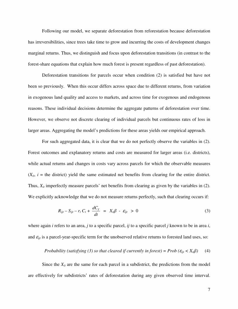
Following our model, we separate deforestation from reforestation because deforestation

has irreversibilities, since trees take time to grow and incurring the costs of development changes

marginal returns. Thus, we distinguish and focus upon deforestation transitions (in contrast to the

forest-share equations that explain how much forest is present regardless of past deforestation).

Deforestation transitions for parcels occur when condition (2) is satisfied but have not

been so previously. When this occur differs across space due to different returns, from variation

in exogenous land quality and access to markets, and across time for exogenous and endogenous

reasons. These individual decisions determine the aggregate patterns of deforestation over time.

However, we observe not discrete clearing of individual parcels but continuous rates of loss in

larger areas. Aggregating the model’s predictions for these areas yields our empirical approach.

For such aggregated data, it is clear that we do not perfectly observe the variables in (2).

Forest outcomes and explanatory returns and costs are measured for larger areas (i.e. districts),

while actual returns and changes in costs vary across parcels for which the observable measures

(Xit, i = the district) yield the same estimated net benefits from clearing for the entire district.

Thus, Xit imperfectly measure parcels’ net benefits from clearing as given by the variables in (2).

We explicitly acknowledge that we do not measure returns perfectly, such that clearing occurs if:

Rijt – Sijt – rt Ct + dCdt

T = Xit� - εijt > 0 (3)

where again i refers to an area, j to a specific parcel, ij to a specific parcel j known to be in area i,

and εijt is a parcel-year-specific term for the unobserved relative returns to forested land uses, so:

Probability (satisfying (3) so that cleared if currently in forest) = Prob (εijt < Xit�) (4)

Since the Xit are the same for each parcel in a subdistrict, the predictions from the model

are effectively for subdistricts’ rates of deforestation during any given observed time interval.

8

The predicted clearing rates depend upon the Xit as well as on the assumed distribution of the εijt.

If the cumulative distribution of εijt is logistic, then we have a logit model for each parcel:

F(Xit�) = 11 exp( )itX β+

(5)

For our grouped data, we estimate this model using the minimum logit chi-square method also

known as “grouped logit”.4 If �hit is an area’s measured rate of forest loss, then we estimate:

log ˆ

ˆ1it

it it

it

hX

hβ µ= +

− (6)

The variance of the µ it (referring to areas, not parcels) can be estimated by 1�

(1 )it it itI h h− , where Iit

represents the number of forested parcels within area i at the beginning of interval t, and the

estimator is consistent and asymptotically normal.5 This is estimated by weighted least squares.

3.2 Poverty, Land Use, and Response To Services Payments

Existing studies of the relationship between poverty and land use have found multiple

linkages although not a single, unambiguous conclusion regarding the direction of causal effects.

Kaimowitz and Angelsen 2002 summarize the economic literature on the causes of deforestation.

They find that income levels, or poverty, have indeterminate theoretical and empirical effects.

Wunder 2001 summarizes the economic literature on poverty and deforestation and concludes

that two effects are in opposition. Capital endowments rise with income, enabling deforestation,

but as returns to other economic activities rise with development, deforestation is less attractive.

Below we consider a number of specific factors that may influence poverty-forest relationships as

prelude to empirically estimating the supply response of land users and in particular the poor.

4 Berkson 1953, cited in Maddala 1983. See also Green 1990 for explicit discussion of heteroskedasticity. 5 Maddala 1983, p. 30.

9

3.2.1 Poverty & Frontiers

Empirical and theoretical studies indicate that population density is positively correlated

with deforestation, fitting the Malthusian vision, though over time density may trigger changes

that lessen pressure on forest, per Boserups’ vision. For the poor unable to compete for choice

jobs or land parcels, increased densities may push them to the agricultural frontier, perhaps far

from markets and perhaps on marginal lands (Kerr et al. 2003b give evidence that poorer areas in

Costa Rica have characteristics that lower returns and thus also clearing). FAO estimates indicate

that tropical forests are home to approximately 300 million people who depend upon shifting

cultivation, hunting and gathering (FAO 1996). Thus the poor may be found near forest frontiers.

This proximity has been noted in citing the potential for carbon services payments to the poor.

Institutional arrangements on frontiers may be dominant conditions for of deforestation.

Remote forests under collective or state ownership that are difficult to monitor can be accessed

without paying for right to use the land. In such areas, the poor may have few options to produce

other than converting forest lands (highly skewed land distribution patterns may support this, as

even on the frontier large fractions of the land may be owned by richer actors who live in cities).

When property titles can be obtained through land clearing, clearing incentives are even stronger.

Thus, the location of the poor may be correlated with forest clearing, but it could be that within a

frontier setting the institutional features are sufficient for clearing, i.e. poverty is not the cause.

A related case is when the creation of new infrastructure, such as roads, generates access

to forest. It may result from public or relatively wealthy private actors, as both transport and

agricultural subsidies for livestock or agricultural production found to be important drivers of

deforestation (Binswanger 1991, Deacon 1994, Chomitz and Gray 1996, Nelson and Hellerstein

1997, Pfaff 1999) may primarily benefit relatively wealth actors such as ranchers and loggers.

10

Small and poor producers may then participate in deforestation on lands abandoned by the large

landowners or on small settlements at the frontier following new roads. A positive correlation of

poverty and deforestation on frontiers may then exist even if poverty is not the main local cause.

3.2.2 Poverty & Barriers To Adopting New Land Uses To Supply Carbon

Poverty has been shown to create a wide array of barriers to adoption of new technologies

in general and in particular to those involving returns that lag investments. Key issues include:

(i) risk; (ii) high costs of capital and lack of investment capacity; (iii) poor property rights; (iv)

transactions costs; and (v) relative efficiency in the production of carbon sequestration to supply.

These factors may cause the supply response of the poor to be lower than that of other land users.

(i) Risk

Productive activities not only generate income or products, they also provide security in

the face of risks of unexpected events like crop failures or sickness. Risks to food security are an

important issue when assessing the opportunity costs of adopting carbon-sequestering land uses.

Giving up the right to ‘liquidate a forest asset’ for needed income during difficult times, e.g., is

potentially an important opportunity cost of receiving payments for carbon services from forests

(for more discussion of such effects of risks the poor face see, e.g., Rodriguez-Meza et al. 2003).

This point has implications for the design of carbon-services payments. If they can be

structured to increase security, as does insurance, they will be more widely adopted. If instead

they represent a new source of uncertainty, then they may be ignored by risk-averse land users.6

A quite different risk issue may also impact the poor. The reversibility of sequestration

activities (e.g., if forests succumb to fire) may cause credits to be discounted as a function of the

6 Lemos et al. 2002, e.g., document a case of potential users not changing land decisions based on rain forecasts.

11

perceived risk of reversal. There are many proposals for handling reversibility, but in any case a

key issue for the poor is that they may be perceived as at higher risk of reversing sequestration.

(ii) Limits On Capital

Poor farmers may not adopt land uses that offer higher productivity over the long term

due to an inability to invest in the short term when resource are required up front. This may be

more relevant for investments in agro-forestry or reforestation than for avoided deforestation.

The poor lack assets and obtaining financial services in the informal sector may be more costly,

discouraging the poor from borrowing to invest (Fafchamps 1999, Lipper 2001). This suggests

that carbon payments programs be structured to help users overcome investment constraints.

(iii) Property Rights

Frequently poor land users do not hold secure individual title to their land. In addition,

more than one type of property right may exist for a given parcel (e.g., rights to trees, water, post-

harvest residue, etc.). Uncertain or complex property rights reduce incentives of land users to

invest in new land uses to sequester carbon, as the private rewards from this will be uncertain.

Sequestration payment programs wishing to include the poor might include rights clarification

when land uses are intended to change, e.g. from pastoral production to agro-forestry activities.

However, this is clearly a challenging area to include within the design of such carbon programs.

(iv) Transactions Costs

Transaction costs are the costs of completing a contract, including the costs for buyers

and sellers to find one another, the costs of bargaining, and the costs of monitoring and enforcing

contracts. High transaction costs for the poor in payments programs can arise from small scale

and remoteness as well as a higher degree of uncertainty in their rights to land-based property.

12

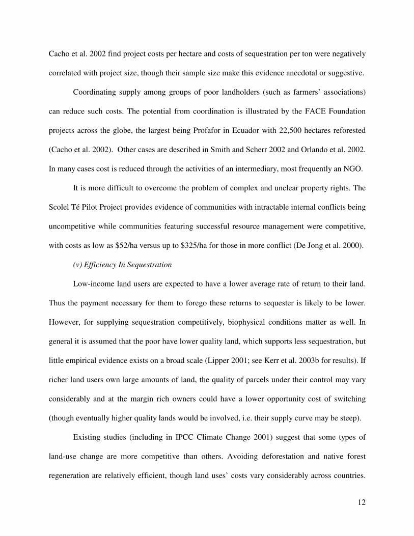
Cacho et al. 2002 find project costs per hectare and costs of sequestration per ton were negatively

correlated with project size, though their sample size make this evidence anecdotal or suggestive.

Coordinating supply among groups of poor landholders (such as farmers’ associations)

can reduce such costs. The potential from coordination is illustrated by the FACE Foundation

projects across the globe, the largest being Profafor in Ecuador with 22,500 hectares reforested

(Cacho et al. 2002). Other cases are described in Smith and Scherr 2002 and Orlando et al. 2002.

In many cases cost is reduced through the activities of an intermediary, most frequently an NGO.

It is more difficult to overcome the problem of complex and unclear property rights. The

Scolel Té Pilot Project provides evidence of communities with intractable internal conflicts being

uncompetitive while communities featuring successful resource management were competitive,

with costs as low as $52/ha versus up to $325/ha for those in more conflict (De Jong et al. 2000).

(v) Efficiency In Sequestration

Low-income land users are expected to have a lower average rate of return to their land.

Thus the payment necessary for them to forego these returns to sequester is likely to be lower.

However, for supplying sequestration competitively, biophysical conditions matter as well. In

general it is assumed that the poor have lower quality land, which supports less sequestration, but

little empirical evidence exists on a broad scale (Lipper 2001; see Kerr et al. 2003b for results). If

richer land users own large amounts of land, the quality of parcels under their control may vary

considerably and at the margin rich owners could have a lower opportunity cost of switching

(though eventually higher quality lands would be involved, i.e. their supply curve may be steep).

Existing studies (including in IPCC Climate Change 2001) suggest that some types of

land-use change are more competitive than others. Avoiding deforestation and native forest

regeneration are relatively efficient, though land uses’ costs vary considerably across countries.

13

Cacho et al. 2002, for four agroforestry systems on degraded lands in Sumatra, found systems

associated with smallholders to be competitive with plantations. Smith and Scherr 2002 note that

costs of carbon from smallholder systems have been quite variable, with the opportunity cost of

the land and scarcity of tree products as a major determinant, and that when smallholder costs are

higher non-carbon benefits may offset this disadvantage. Tomich et al. 2001 studied in detail the

costs of carbon sequestration in land-use systems in Sumatra and found competitive smallholder

sequestration but questions about relative profitability. These questions will require further study.

4. DATA

Below we describe the forest, poverty and economic returns variables that we use to empirically

examine the linkages between service payments and poverty and ongoing rates of deforestation

(for a summary of Costa Rican clearing, and further details about the data, see Kerr et al. 2003a).

4.1 Deforestation Variable

We observe forest cover at five points in time (1963, 1979, 1986, 1997, 2000). We use

the separation of the country into 436 political districts, and can use as unit of observation a form

of sub-district. Specifically, in each district we can distinguish each ‘lifezone’ that is present (the

Holdridge Life Zone System (Holdridge 1967) divides Costa Rica into twelve ecological

‘lifezones’ reflecting levels of precipitation and temperature). On average there are about three

lifezones present in a district and thus we can in principle use up to 1229 observations per year,

although because the poverty index described below is for districts, we will focus upon districts.

Our dependent variable (more below) is the annual percentage loss during a given time interval

from the area of forest present within a given district-lifezone at the beginning of the interval. As

some district-lifezones become fully deforested, over time the observations per interval fall.

14

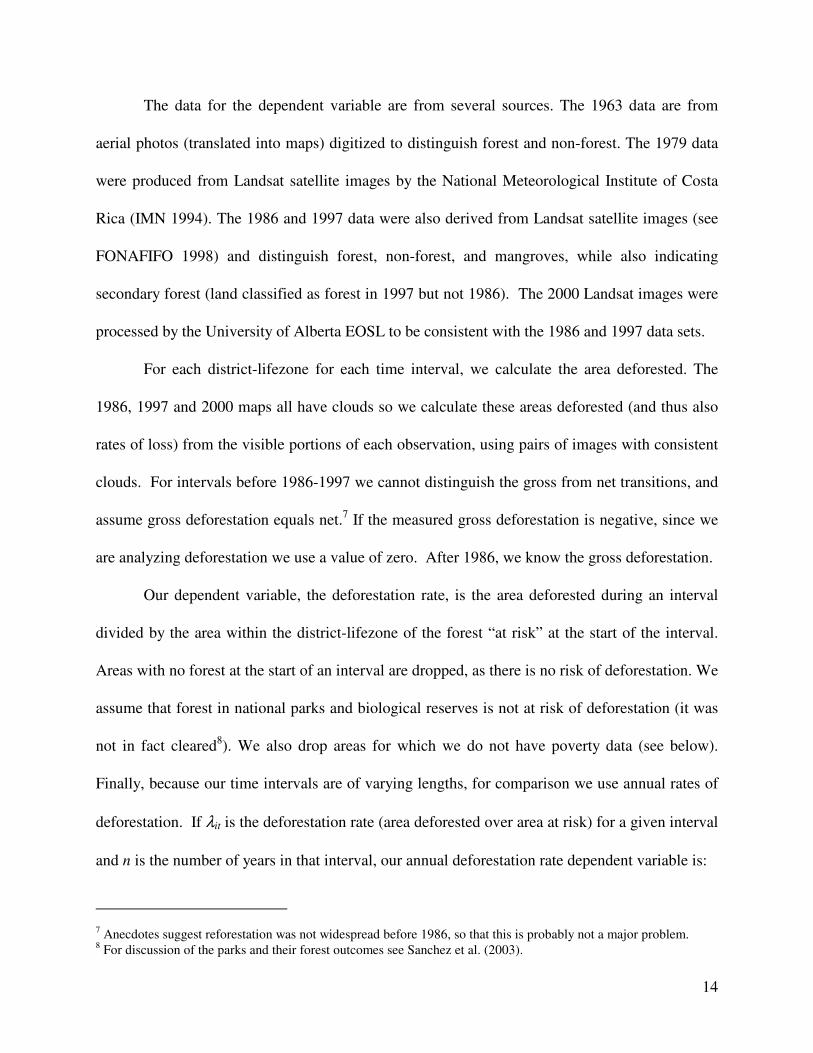
The data for the dependent variable are from several sources. The 1963 data are from

aerial photos (translated into maps) digitized to distinguish forest and non-forest. The 1979 data

were produced from Landsat satellite images by the National Meteorological Institute of Costa

Rica (IMN 1994). The 1986 and 1997 data were also derived from Landsat satellite images (see

FONAFIFO 1998) and distinguish forest, non-forest, and mangroves, while also indicating

secondary forest (land classified as forest in 1997 but not 1986). The 2000 Landsat images were

processed by the University of Alberta EOSL to be consistent with the 1986 and 1997 data sets.

For each district-lifezone for each time interval, we calculate the area deforested. The

1986, 1997 and 2000 maps all have clouds so we calculate these areas deforested (and thus also

rates of loss) from the visible portions of each observation, using pairs of images with consistent

clouds. For intervals before 1986-1997 we cannot distinguish the gross from net transitions, and

assume gross deforestation equals net.7 If the measured gross deforestation is negative, since we

are analyzing deforestation we use a value of zero. After 1986, we know the gross deforestation.

Our dependent variable, the deforestation rate, is the area deforested during an interval

divided by the area within the district-lifezone of the forest “at risk” at the start of the interval.

Areas with no forest at the start of an interval are dropped, as there is no risk of deforestation. We

assume that forest in national parks and biological reserves is not at risk of deforestation (it was

not in fact cleared8). We also drop areas for which we do not have poverty data (see below).

Finally, because our time intervals are of varying lengths, for comparison we use annual rates of

deforestation. If λit is the deforestation rate (area deforested over area at risk) for a given interval

and n is the number of years in that interval, our annual deforestation rate dependent variable is:

7 Anecdotes suggest reforestation was not widespread before 1986, so that this is probably not a major problem. 8 For discussion of the parks and their forest outcomes see Sanchez et al. (2003).

15

� ( )hit itn= − −1 11

λ (7)

Thus we implicitly assume that this annual deforestation rate was constant during each interval.

4.2 Explanatory Variables

4.2.1 Direct Measure of Economic Returns

The annual return rjkt to a given hectare j in crop k at time t is the crop price pkt times the

annual yield per hectare yjkt minus the costs of production costjkt minus the transport cost tjkt. For

each year, we estimate the returns for the four major export crops: coffee, bananas, sugar and

beef. We have data from 1950 onward although its quality improves significantly in later years.

For each interval, returns are averaged across the years for an average return (in 1997 US$) to

crop k on one hectare of cleared land during that interval (see Appendix on data and techniques).

Any parcel is used for one crop at a time. We define sjk as the probability of a crop being

chosen as the use of newly cleared land. For larger areas, these probabilities imply expected

shares of the area in each crop, to be used as weights in our measure of expected annual return:

Rit = E(rijt) = jk jktk

s r� (10)

We calculate the sjk using data on production patterns in the 1970s and 1980s and information on

the suitability of different lifezones for different crops. For example, in a humid, lower-montane

area we represent land choices by assuming that cleared land will be used for coffee or a similar

return. The resulting Rit is our returns measure, AGRETURN. Higher returns should raise clearing,

such that payments for forest that lower relative returns to agriculture would lower deforestation.

4.2.2 Poverty Index

Here we summarize Cavatassi et al. 2003’s poverty index estimation for Costa Rica.

Without sufficient household-level data for a ‘small area estimation’ approach, they chose to use

16

‘principal components analysis’ (PCA). The necessary data are available from the census over

four decades, permitting a poverty index that can be matched with the deforestation observations.

The data are variables common to multiple censi, at district level. Seventeen variables are

common to 1973, 1984, and 2000, of which twelve are common to the 1963 census as well. See

Cavatassi et al. 2003 for discussion of judgments about variables’ economic meanings and roles

in explaining the overall variance in these data. Variables chosen include demographic, labor,

education, housing, infrastructure and consumer durable variables. Some examples are the

percentage of dwellings without heaters, or without bathrooms, or without electricity. Others are

the average number of occupants per bedroom and percent of people receiving job remuneration.

In PCA, eigenvectors of the correlation matrix for these variables indicate the direction

and weight of variables in the index. Cavatassi et al. 2003 find that greater values of variables

that should be positive correlated with poverty (% with dirt floor, % without refrigerators) have

positive signs in the poverty index, as expected, while the wage remuneration and education

variables have negative signs, as makes sense. The weights are used to create a poverty index9:

Marginality (or Poverty) Indexj = W1*(aj1-a1)/(s1) + ...... + Wn*(ajn-an)/(sn) (8)

where W is the weight for a variable (among variables 1 to n in (8)), aj is the jth district's value for

that variable and a and s are the mean and standard deviation of the variable across the districts.

This method is first used to create year-specific poverty indices for 1963, 1973, 1984 and

2000. Such indices, however, are not comparable over time. Each is based on a scale relevant

only to that year. In other words, the indices’ units vary, precluding comparison between years.

Thus, as a second step, Cavatassi et al. 2003 also pool all years’ data to estimate a single PCA for

1973-2000 using the seventeen variables and one for 1963-2000 using the twelve variables. For

17

these pooled PCA estimations, a change in the marginality index arises only from changes in the

levels of variables over time, not changes in the relative importance of each variable in the index.

As noted above, some observations must be dropped because of a lack of poverty data.

The reason is that the number of districts changes each census year (from 334 in 1963 to 406 in

1973, to 459 in 2000) as older larger districts are split to form newer smaller districts. When they

knew how such a split has occurred, Cavatassi et al. 2003 are able to use the poverty values for

older larger districts for each of the smaller newer districts into which they split. However, for

some districts they were unable to track these changes over time, and thus districts are dropped.

Finally, we make use of these indices in our regressions in a number of ways. First, we do

work with both the 1963-2000 and the 1973-2000 indices to explore the tradeoff between more

variables and more observations over time. We match this data to our intervals as follows. For

the 1963-2000 measure, for 1963-1979 we use the 1963 values, while for 1979-1986 we use the

1973 values, for 1986-1997 we use the 1984 values and for 1997-2000 we use the 2000 values.

We also try using the 1984 values for the 1997-2000 interval so that we are using lagged values.

For the 1973-2000 measure the difference is that for 1963-1979 we have only the 1973 values.

A final matching step is to the 436-district structure used by the University of Alberta to

organize the forest data and some explanatory data (some data are spatially specific, so that they

can be parsed into any district structure within a GIS). For years before 2000 we must match the

smaller number of census districts to these 436 while for 2000 we match the 459 districts to 436.

We use the indices directly, in their continuous form, but also create variables to reflect

possible non-linear relationships (logarithms, quartiles) between poverty and deforestation since

some of the theory concerning poverty’s effect concerns extreme poverty, e.g. pure subsistence.

9 This formula is based upon Filmer and Pritchett 1998.

18

5. Carbon Supply from Avoided Deforestation: Empirical Results

In the following section, we present empirical estimates of the relationship between poverty and

the potential supply response to sequestration payments for Costa Rica. We draw also upon the

empirical results in Kerr et al. 2003b (which estimates poverty’s direct and indirect effects on

deforestation) for a land-use baseline in the absence of environmental services payments. This we

can convert to a carbon baseline using the estimated carbon values presented in Table 1 below.

5.1 Carbon Supply In Response To Payments

Table 2’s column I presents our first result to address the issue of whether environmental

services payments should be expected to induce changed land uses and sequestered carbon. The

significance of returns is evidence that the relative returns to forested land uses do affect clearing.

It is worth noting the absence of other variables in this regression. Since our returns

measure, as noted, certainly does not capture all possible elements of actual returns, we might

wish to include variables controlling for potentially omitted elements. For instance, as transport

costs are notably missing from our direct returns measure, we might include the proxy for access

to markets from Kerr et al. 2003a, the distance to the closest of three major Costa Rica markets.

However, all regressions in Table 2 include district fixed effects. These control for fixed

differences, such as distances to major markets, but mean that we can not separately include the

factors in clearing which vary only over space such as distances and other important factors such

as fixed ecological conditions. However, again, fixed effects control for their effects. Further,

they will also control for the effects of fixed spatial differences that we can not directly observe.

Given this result that payments can induce carbon supply, and the fact that some land

users who could potentially deforest are poor, we can imagine that the hypothetical ‘win-win’ is

19

feasible. Carbon-services payments could generate environmental gains and lessen rural poverty.

Whether to target the poor or not, e.g. because they respond more or less, is another question.

5.2 Carbon Supply by the Poor: Baselines & Poverty’s Effect On Supply

5.2.1 Poverty’s Direct & Indirect Effects on Deforestation

Below, in section 4.2.2, we examine whether deforestation in poor areas is more or less

responsive to carbon rewards. Even for the same rate of deforestation, however, because poorer

areas contain a large share of the forest, they are responsible for more clearing and, similarly,

with the same responsiveness to carbon payments they would supply more total sequestration.

One reason that more forest remains in those areas appears to be that the characteristics of

the land in poorer areas are less favorable for earning returns from cleared land uses like crops.

Kerr et al. 2003b, e.g., provide evidence that the difference between poorer and richer districts in

characteristics that affect deforestation would lead to lower deforestation rates in poorer areas.

However, controlling for observed and unobserved land characteristics, Kerr et al. 2003b

find that poverty raises deforestation. Figure 1’s baseline simulation of deforestation and carbon

storage is based on this, with a poverty effect consistent with our Table 2 below, which focuses

on the effects of returns and the interactions of returns with poverty that we explore below.

5.2.2 Poverty Effect On Supply Response

Columns II through IV of Table 2 bring poverty indicators into the supply regressions,

employing the 1963-2000 measure using its 1963, 1973, 1984, and 2000 value for the intervals.

The first result of interest is that, as in Kerr et al. 2003b, controlling with fixed effects (i.e., for

observed and unobserved characteristics of land), poorer areas have higher deforestation rates.

Columns III and IV, though, present the evidence that is novel and of greatest interest.

The interaction term for poverty and returns is negative and significant. This suggests that poorer

20

people will respond less to carbon payments, as seen in Figure 1 (this type of result arises for the

other continuous poverty indices as well, but is less strong for the poorest-quartile dummies).

Column IV conveys that including other controls, i.e. other factors that affect deforestation rates

(see Kerr at al. 2003a for extended discussion of the past clearing variable and its interpretation),

leaves the interaction term essentially unchanged. As noted, because we are using fixed effects

to control for fixed differences across district-lifezones, we do not include other fixed factors that

affect deforestation, such as a distance proxy for market acces or fixed ecological conditions.

This result suggests a lack of empirical basis for focusing carbon payments programs on

the poor if the goal is efficient generation of carbon sequestration (of course, if a program directly

favors poverty reduction as an objective, then targeting the poor will remain the obvious choice).

Even should the poor be more desperate for marginal income than those with greater wealth, as

noted above they may face a range of barriers to switching land uses which discourage supply.

On the other hand, this interaction is not a large effect and in general land users will respond. The

Discussion section below considers further the potential for the poor to receive carbon payments.

5.3 Simulating Carbon Baselines & Carbon Supply

Though we have already referred to the figures, from our simulations of carbon outcomes,

here we explain our simulations. To calculate carbon we multiply the amount of forest in each

district by the amount of carbon that district’s forest can potentially store. The carbon storage

numbers used in this study are given in Table 1. For further explanation, see Kerr et al. 2003c.

We then forecast deforestation when net returns to land clearing are lower by the amount

of the carbon return (i.e., carbon price x carbon/hectare). Our predictive equation becomes:

21

)())(__(

),()(1

ln)(

tDihapercarbonpricecarbonreturns

itxixh

hty

treturns

dynamicdstatics

��

��

+×−+

+=

��

���

�

−=

ββ

ββ

where h is the measured district-lifezone deforestation rate, xstatic are the solely spatially varying

explanatory variables (distances, lifezones, soils), xdynamic are spatially and temporally varying

explanatory variables, D(t) is a function of time estimated using a time-dummies version of the

regression in question from Table 2, and β are all of their regression-estimated coefficients.

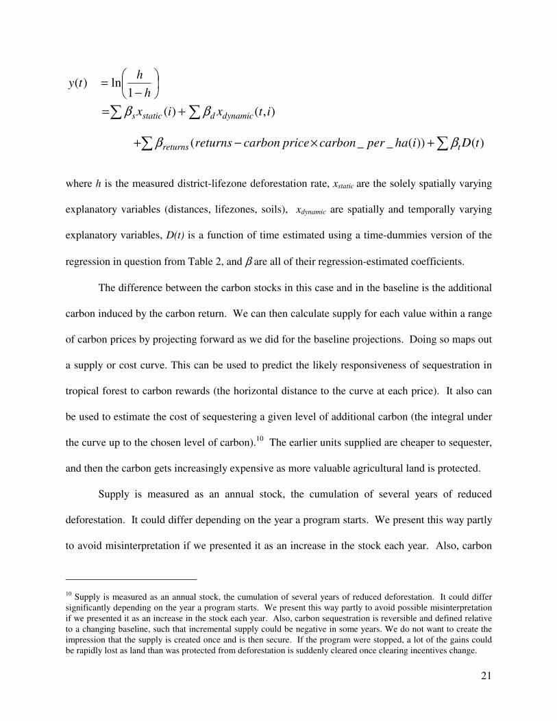
The difference between the carbon stocks in this case and in the baseline is the additional

carbon induced by the carbon return. We can then calculate supply for each value within a range

of carbon prices by projecting forward as we did for the baseline projections. Doing so maps out

a supply or cost curve. This can be used to predict the likely responsiveness of sequestration in

tropical forest to carbon rewards (the horizontal distance to the curve at each price). It also can

be used to estimate the cost of sequestering a given level of additional carbon (the integral under

the curve up to the chosen level of carbon).10 The earlier units supplied are cheaper to sequester,

and then the carbon gets increasingly expensive as more valuable agricultural land is protected.

Supply is measured as an annual stock, the cumulation of several years of reduced

deforestation. It could differ depending on the year a program starts. We present this way partly

to avoid misinterpretation if we presented it as an increase in the stock each year. Also, carbon

10 Supply is measured as an annual stock, the cumulation of several years of reduced deforestation. It could differ significantly depending on the year a program starts. We present this way partly to avoid possible misinterpretation if we presented it as an increase in the stock each year. Also, carbon sequestration is reversible and defined relative to a changing baseline, such that incremental supply could be negative in some years. We do not want to create the impression that the supply is created once and is then secure. If the program were stopped, a lot of the gains could be rapidly lost as land than was protected from deforestation is suddenly cleared once clearing incentives change.

22

sequestration is reversible and defined relative to a changing baseline, such that incremental

supply could be negative in some years. We do not want to create the impression that the supply

is created once and is then secure. If the program were stopped, a lot of the gains could be

rapidly lost if land protected from deforestation were suddenly cleared once incentives ended.

Figures 1 and 2 provide two ways to see the implications of Table 2’s land-use results

when they are jointed with the carbon-per-unit-forest values in Table 1. Both follow from the

results in column III of Table 2. Figure 1 conveys that payments that change agricultural returns,

relative to returns to standing forest, will increase the carbon stock retained in forests over time

yet also that the poor are estimated to be less responsive to payment. This makes a difference.

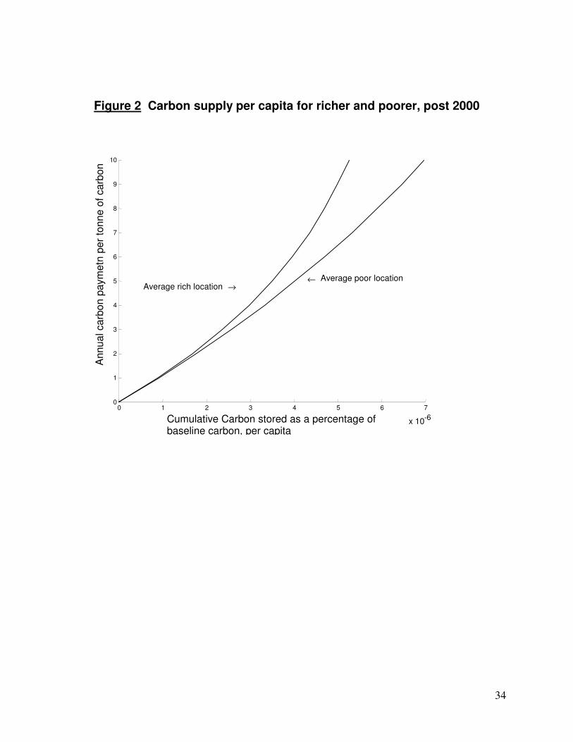
Figure 2 is different in two ways, conveying some of the different ways to view results of

this kind. First, it presents actual carbon supply curves, i.e. levels of increase in carbon storage

relative to the baseline, in both poorer and richer areas, as a function of the level of the payment.

This demonstrates the kind of information that could inform decisions about whether or not to

participate in a market for carbon services, as the potential benefits can be computed in advance.

Second, it presents the results on a per capita basis. The fact that there is more forest per

capita in the poorer areas is seen in Figure 2 to outweigh the lower responsiveness of the clearing

in poorer areas. This raises again the idea that payments policies could potentially provide some

significant benefit to the poor while protecting forests, something that we discuss further below.

6. Discussion

In this paper, we adopted a revealed preference approach to estimating both the potential supply

response to sequestration payments and the effects of poverty upon the level of responsiveness.

We used data on Costa Rican forests for five points in time along with a poverty index from FAO

23

to estimate responsiveness and to simulate the supply of avoided deforestation for Costa Rica,

finding that, in general, land users will respond to payments, and that the poor will respond less.

This is consistent with findings from the literature on general agricultural response to incentives.

Despite the latter result, since users respond in general, some land users are poor, and much of

the forest is in poorer areas, there seems to be potential for payments that would at once support

the conservation of forests and effect transfers to poorer people to address concerns about equity.

A caveat concerning transfers to the poor concerns the current details of the CDM.

Avoided deforestation, as noted, is currently excluded from the activities that generate credits.

Thus being in an area with a lot of forest and keeping it in forest would not be rewarded with

carbon-services payments under the CDM. This limits the advantage, with respect to carbon

payments, that the location of much of the forest within poorer areas could otherwise convey.

Considerable work remains to finalize the rules under which sequestration programs such

as the CDM will operate. The way these are settled is likely to have considerable importance for

the potential of such programs to reach the poor. Another key issue for the poor in the adoption

of a new technology, such as changing land use for payments, is the risk within the policy design.

A risk that arises in the market for carbon sequestration services comes from the

uncertainty of actual sequestration levels meeting projected sequestration potential. Thus land

users may enter into a sequestration agreement but find that they have not met expected levels,

even though they have followed recommended practices. In addition, the setting of the baseline

involves some uncertainty, particularly if these are allowed to be updated over time as proposed.

The way in which carbon contracts are designed and monitored will determine to what

extent this risk will be shared between buyers and sellers. If land users are paid on a per hectare

basis for the adoption of practices, the seller would assume the risk of falling short. Alternatively

24

of land users are paid for carbon sequestered they assume the risk. The efficiency of adopting

either scheme will be determined by the relative costs associated with monitoring land use

practices versus monitoring carbon tonnage, as well as the heterogeneity of biophysical and

economic conditions which impact sequestration supply. (Antle & McCarl 2001). In terms of the

potential impact on poor land users' participation in carbon markets, the adoption of contracts

based on a per hectare adoption of land use practices is clearly more beneficial. Poor land users

are unlikely to be capable of bearing the risk associated with carbon supply shortfalls.

Finally, an important caveat is necessary, given that our data on poverty and clearing are

not for households but for districts. It is possible that even in poorer areas, where a large fraction

of the inhabitants may be relatively poor, those who own the land are not nearly as poor. Should

that be the case, then if services and service payments are roughly proportional to land holdings

the payments flowing to poorer areas would not be received by the poorest people. Such a

situation with respect to land ownership could hinder efforts to support forests and equity. This

suggests the value of repeating exercises such as that carried out here but using household data.

In sum, payments for environmental services can be an important way in which poor land

users can be assisted while contributing to global goals. But there may be conflicts between the

multiple goals many have in mind for such payments programs. Projects maximizing poverty

alleviation may be quite different from projects maximizing carbon sequestration. For efficiency

of the latter, more about the distribution of sequestration potential can help, as would information

on when provision of environmental goods and services also yields private production benefits to

farmers. In those settings, required payments should be lower. And leveraging carbon payments

with payments for other environmental services could be efficient.

25

However, both equity and efficiency goals were intended within the agreements reached

at Rio in 1990. The idea then was that it is neither fair nor effective to demand the provision of

environmental services from the poor unless this also offers the potential for better livelihoods.

But for this to be the case, more focus on that goal and efforts to achieve it will be necessary.

The analysis presented in this article suggests that poor land users are not necessarily

going to be the major beneficiaries of environmental services payments. Nonetheless, carbon

sequestration payments could help to address poverty while also satisfying others’ environmental

goals, which could function as a new means of financing rural development efforts. But again,

for this to occur focused efforts will be necessary. Structuring payment programs to address the

insurance needs of the poor and their investment constraints is one important means to promote

poor land user participation in environmental service payment programs. Facilitating group

coordination of land management and strengthening property rights institutions is another key

measure that may be needed to channel benefits of environmental service provision to the poor.

26

References

Antle, J. M. and McCarl, B., 2001, The Economics of Carbon sequestration in Agricultural Soil,

in Volume VI of the International Yearbook of Environmental and Resource Economics,

edited by Tom Tietenberg and Henk Folmer, published by Edward Elgar

Ball, Jeffrey. April 16, 2003 Wall Street Journal “Global Warming is Threat to Health to

Corporations” Section A. Pg. 2.

Beckerman, W., 1995, Small is stupid - Blowing the Whistle on the Greens. London, Duckworth.

Bass, S., O. Dubois, J. Ford, P. Moura-Costa, M. Pinard, R. Tipper, C. Wilson (1999) Rural

Livelihoods and Carbon Management: An Issues Paper available for download from

http://www.ecosecurities.com

Black_Arbelaez, 2002, Applying CDM to Biological Restoration Projects in Developing

Nations: Key Issues for Policy Makers and Project Managers, available at:

http://www.gefweb.org/documents.pdf

Callaway, J.M. and McCarl, Bruce. The Economic Consequences of Substituting Carbon

Payments for Crop Subsidies in U.S. Agriculture. Environmental and Resource

Economics, January 1996, 7(1), pp 15-43.

Chomitz, K. E. Brenes, L. Constantino “Financing environmental services: the Costa Rican

experience and its implications” The Science of the Total Environment 240 (1999) 157-

169

Ciesla, W.M., 1995, Climate change, forests and forest management: an overview, in: FAO

Forestry Paper, (FAO), no. 126 / FAO, Rome (Italy).

Committee on Abrupt Climate Change, O. S. B., Polar Research Board, Board on Atmospheric

Sciences and Climate, National Research Council (2001). Abrupt Climate Change:

Inevitable Surprises. Washington D.C., National Academy Press.

Ehrlich, P.R. and Ehrlich, A.H., 1996, Betrayal of Science and Reason - How anti-

Environmental Rhetoric Threatens Our Future, Washington D.C.: Island Press.

GTZ, Deutsche Gesellschaft für Technische Zusammenarbeit, (2001), On track towards climate

protection. Eschborn, Germany.

Harrison, Susan 1991 Population Growth, Land Use and Deforestation in Costa Rica, 1950-1984

Interciencia March-April 1991 Vol. 16 No. 2 pp. 83-93

27

Intergovernmental Panel on Climate Change, IPCC, (2001b). The Science of Climate Change

2001. Report of the Working Group I. Available on line at:

http://www.usgcrp.gov/ipcc/default.html

Intergovernmental Panel on Climate Change, IPCCC, (2001a). Climate change 2001: Impacts,

Adaptations, and Vulnerability. Report of the Working Group II. Available on line at:

http://www.usgcrp.gov/ipcc/default.html

Kerr, Suzi (2001) “Seeing the Forest and Saving the Trees: tropical land-use change and global

climate policy” in Can Carbon Sinks Be Operational? RFF Workshop Proceedings,

Roger A. Sedjo and Michael Toman July 2001 Resources for the Future Discussion Paper

01–26 www.rff.org

Kerr, S., A.S.P. Pfaff and G.A. Sanchez-Azofeifa (2003a). “Development and Deforestation:

evidence from Costa Rica”. Requested revision resubmitted (and see www.motu.org.nz).

Kerr, S., A.S.P. Pfaff, R. Cavatassi, B. Davis, L.Lipper, G.A. Sanchez-Azofeifa, and J. Timmins

(2003b). “Effects of Poverty on Deforestation: distinguishing location from behavior”.

Kerr, S., J. Hendy, S. Liu, A.S.P. Pfaff (2003c). “Uncertainty and the Contribution of Tropical

Land-use to Carbon Mitigation”.

Kishor, N.M. and Constantino L.F. 1993 Forest Management and competing land uses: and

economic analysis for Costa Rica, World Bank: LATEN dissemination note no. 7, 1993

cited in Kenneth Chomitz, E. Brenes and L. Constantino 1999 “Financing environmental

services: the Costa Rican experience and its implications” The Science of the Total

Environmentl 240 (1999) 1570169.

Lal, R., Kimble, J. M., Follett, R.F. and Cole, C.V., 1998, The potential of US cropland to

Sequester Carbon and Mitigate the Greenhouse Effect, Chelsea, MI: Ann Arbor Press.

Levia, D. F. 1999. Land degradation: Why is it continuing? Ambio 28(2):200-201.

Meyers, N. and Simon, J., (1994). Scarcity or abundance? A debate on the environment. New

York, W.W. Norton.

Nasi, Robert, Sven Wunder and Jose J. Campos (2002) “Forest Ecosystem Services: Can They

Pay Our Way Out of Deforestation?” Discussion paper prepared for GEF for the Forestry

Roundtable New York, March 11, 2002. Available at

http://www.gefweb.org/documents.pdf

28

National Research Council (NRC), (2001). Climate Change Science: An analysis of some key

questions. Washington, D.C., National Academy Press.

Parks, Peter J. and Ian W. Hardie (1995) Least Cost Forest Carbon Researves: Cost-Effective

Subsidies to Convert Marginal Agricultural Land to Forests. Land Economics 71(1):

122-36

Plantinga, Andrew, Thomas Mauldin and Douglas Miller 1999 An Econometric Analysis of the

Costs of Sequestering Carbon in Forests American Journal of Agricultural Economics

81 pp. 812-824.

Simon, J. L. (1995). The State of Humanity. Cambridge (Mass.), Blackwell.

Stavins, R. 2000. The costs of carbon sequestration: A revealed preference approach. American

Economic Review.

Tipper Richard (1996), Mitigation of Greenhouse Gas Emissions by Forestry: A Review of

Technical, Economic and Policy Concepts, Working paper, Institute of Ecology and

Resource Management, University of Edinburgh, Scotland.

More References

Aguilar, J., Carlos Barboza, and Jorge Leon. 1982a. Desarollo tecnologico del café en Costa

Rica y las politicas cientifico tecnologicas. Consejo Nacional de Investigaciones Cientificas

y Tecnologicas, Costa Rica.

———. 1982b. Desarollo tecnologico en la ganaderia de carne. Consejo Nacional de

Investigaciones Cientificas y Tecnologicas, Costa Rica.

Arias, Jose, and Rafael Corrales. 1992. El sub-sector carne (ganaderia bovina) de Costa Rica, su

sistema agroindustrial, comportamiento, limitaciones y fortalezas del mismo. Taller de

Evaluacion Economica Centro de Politicas y Economia Aplicada, INCAE.

Barboza, Carlos V., Justo F. Aguilar, and Jorge S. León. 1982. Desarollo tecnologico en el

cultivo de la caña de azucar . Consejo Nacional de Investigaciones Cientificos y

Tecnologicas, Costa Rica.

Chaves-Solera, M. A. 1994. Organizacion de la agroindustria azucarera costarricense y costos

de produccion agricola de la caña de Azucar. DIECA 59p. San Jose, Costa Rica.

29

Chavez-Solera, M. A., et al. 1998. Area cultivada y rendimientos agrícolas de la caña e azúcar en

Costa Rica. 12th Congreso de ATACORI.

de Graaf, F. 1986. The economics of coffee. Economics of crops in developing countries no. 1

Wageningen: Dudoc.

Consejo Nacional de Produccion, Costa Rica. Unidad de analisis de politicas, carne de vacuno

“Principales variables estadisticas 1980–1995.”

Mendez, Nora Bermudez, and Rosa Maria Pochet Coronado. 1979. La agroindustria de la caña de

azucar en Costa Rica: Modificaciones economicas y sociales (1950–1975). Informe de

Investigacion, Confederacion Universitaria Centro Americana ESUCA Program

Centroamericano de Ciencias Sociales

Ramos Mendez, R. A., and Aguzzi G. Brenes. 1997. Distribucion de la produccion de café por

cantones y provincias, cosecha 1996–1997. Instituto del Café de Costa Rica: Departmento de

Estudios Agricolas Economicos y Liquidaciones.

Vargas, J.R. and O. Saenz. 1994. Costa Rica en cifras 1950–1992. MIDEPLAN PNUD.

Vigne, Alain. 1974. Costos de produccion en ganado de carne Costa Rica. Ministerio de

Agricultura y Ganaderia: Departmento de Economia y Estadisticas Agropecuarias. San Jose,

Costa Rica.

30

Appendix – direct measure of returns from beef, coffee, sugar and bananas

Units: crop price is in $/kg; yield is in kg/ha; production cost is in $/ha; transport cost is in $/ha.

Observations: 436 districts in Costa Rica from 1900-1997 in principle, but 1950-1997 in fact. The limitations on historical data mean that we do not have good measures for years before 1950 and more generally even within 1950-1997 the quality of the data is higher for the later intervals.

Prices: though some production is sold domestically, Costa Rica is a small country and we use exogenous export prices (in 1997 US$). Price data are taken from two sources, the Costa Rican Ministry of Planning (Vargas and Saenz 1994) and the Central Bank of Costa Rica website. Yields: crop yields vary over time because of technological change, and across space because of differences in general productivity and in suitability for particular crops. While lifezones and soils proxy for this variability, here we estimate yield. For instance, in some areas the yield for a particular crop is effectively zero since it would never be grown there. Our data is of two types.

For some crops we have data on yield per hectare: for bananas, county level for 1977-1997, and given no obvious trend we assume this to be constant before 1977; for sugar, province level for several years between 1950 and 1977 and for county level in 1998, and we apply the province-level trends to extrapolate the yields for all counties within a province before 1998. Else we observe production (kg) and area in production (ha) and divide to get the yields. For coffee we have production from 1974-1992 and 1996 at county level and area at county level from the census for 1950, 1955, 1963, 1973, and 1986. We assume production is fixed pre-1974 and area is fixed post-1986, and then interpolate the coffee areas before calculating yield ratios. For pasture we use national production from 1950 to 1995 and divide by census estimates of area for a national yield estimate. We create county-level variation by utilizing the ratio of number of cattle to pasture in the census data, assuming this variation is related to productivity. In locations where the yields for particular crops are undefined within our data, we assume that they are zero.

Costs: we estimate operating costs on an annual basis, although the data are sparse. For coffee, we observe costs only in 1979 and 1981 by coffee zone. For beef we have a single reliable estimate from 1974 at the national level. For sugar, data is better although still at national level, with estimates from Barboza, Aguilar, and León 1982 and Chaves-Solera 1994 for 1963, 1966, 1972, 1977, 1979 and 1994–96. For bananas we have a technical estimate from Hengsdijk (personal communication, Wageningen Agricultural University) for 1997, but no previous data. These are assumed constant outside the period within which they are observed and interpolated. For transport costs, lacking direct measures, currently we rely upon the proxy described above.

Crop Shares: to predict how likely each of the four crops is to be chosen, we use a combination of census and satellite land-use data to estimate the share of each crop in each district. While the satellite data are more precise, they distinguish not crops but simply land uses (permanent crops, pasture, and forest). The data is from 1973 and 1984, and our shares do not change over time.

We combine the district shares with the crop returns for expected annual return per district-year, following (6) above. Then we average the returns across intervals to generate mean returns to which we assume our estimated constant annual interval deforestation rate will have responded.

31

Table 1 Carbon Stocks by Lifezone

GEMS Life zone

Mean Std dev as % of mean

Premontane moist 159 43%

Lower montane moist 134 45%

Tropical Moist 156 24%

Premontane wet 156 32%

Lower montane wet 113 54%

Montane wet 119 34%

Tropical Wet 336 40%

Tropical Dry 96 41%

Premontane rain 120 49%

Lower montane rain 116 58%

Montane rain 96 86%

We estimate potential carbon storage in primary forests with the General Ensemble Biogeochemical Modeling System (GEMS) that incorporates spatially and temporally explicit information of climate, soil, and land cover (Liu et al. 2002a; Liu et al. 2003). GEMS is a modeling system that was developed for a better integration of well-established ecosystem biogeochemical models with various spatial databases for the simulations of the biogeochemical cycles over large areas. The well-established model CENTURY (Parton et al. 1987; Schimel et al. 1996) was used as the underlying plot-scale biogeochemical model in this study. It uses a Monte-Carlo-based ensemble approach to incorporate the variability (as measured by variances and covariance) of state and driving variables of the underlying biogeochemical models into simulations. The mean values and their corresponding standard deviations of aboveground biomass carbon density simulated by GEMS are listed in Table 1.

32

Table 2 Regression results used as basis of supply simulations

Grouped Logit

I II III IV

Dependent

Variable

annualised

def. prob.

annualised

def. Prob.

annualised

def. prob.

annualised

def. prob. Explanatory Variables

Coefficients

(standard error)

RETURNS .00010 (2.8)

.00009 (1.4)

.00011 (1.6)

.00009 (1.4)

POVERTY 0.13 (2.6)

0.17 (3.2)

0.17 (3.2)

RETURNS * POVERTY -.00008 (-2.9)

-.000066 (-2.5)

%CLEARED 1.2 (1.3)

%CLEARED2 -3.3 (-3.5)

TIMEDUMMY 1979-1986

0.55 (10)

0.88 (8.3)

0.95 (8.8)

1.1 (8.8)

TIMEDUMMY 1986-19972

-0.51 (-7.4)

-0.24 (-1.3)

-0.18 (-0.98)

0.095 (0.44)

TIMEDUMMY 1997-2000

-1.6 (-13)

-1.4 (-4.6)

-1.4 (-4.8)

-1.1 (-3.6)

CONSTANT -3.2 (-110)

-3.6 (-18)

-3.7 (-18)

-3.5 (-16)

FIXED EFFECTS F = 7.8 (P = 0.00)

F = 7.8 (P = 0.00)

F = 7.8 (P = 0.00)

F = 6.4 (P = 0.00)

ADJUSTED R2 0.69 0.74 0.75 0.76

N 1621 973 973 973

Coefficients reported with t statistics below them in parentheses (except for the fixed effects, where F reported above with P value below).

33

Figure 1 -- Carbon outcomes for richer and poorer districts in response to a $10 annual carbon payment, post 2000

2000 2002 2004 2006 2008 2010 2012 2014 2016 2018 2020 85

90

95

100

Year

Tota

l car

bon

(cum

ulat

ive)

as

% o

f car

bon

stoc

k in

200

0

Average rich location ←

Average poor location ←

Baseline ←

34

Figure 2 Carbon supply per capita for richer and poorer, post 2000

0 1 2 3 4 5 6 7 x 10 -6

0

1

2

3

4

5

6

7

8

9

10

Cumulative Carbon stored as a percentage of baseline carbon, per capita

Ann

ual c

arbo

n pa

ymet

n pe

r to

nne

of c

arbo

n

Average poor location ← Average rich location →

35

ESA Working Papers

WORKING PAPERS The ESA Working Papers are produced by the Agricultural and Development Economics Division (ESA) of the Economic and Social Department of the United Nations Food and Agriculture Organization (FAO). The series presents ESA’s ongoing research. Working papers are circulated to stimulate discussion and comments. They are made available to the public through the Division’s website. The analysis and conclusions are those of the authors and do not indicate concurrence by FAO. ESA The Agricultural and Development Economics Division (ESA) is FAO’s focal point for economic research and policy analysis on issues relating to world food security and sustainable development. ESA contributes to the generation of knowledge and evolution of scientific thought on hunger and poverty alleviation through its economic studies publications which include this working paper series as well as periodic and occasional publications.

Agricultural and Development Economics Division (ESA)

The Food and Agriculture Organization Viale delle Terme di Caracalla

00100 Rome Italy

Contact: Office of the Director

Telephone: +39 06 57054358 Facsimile: + 39 06 57055522 Website: www.fao.org/es/esa

e-mail: ESA@fao.org