NBER WORKING PAPER SERIES

WHY HAVE COLLEGE COMPLETION RATES DECLINED? AN ANALYSIS OFCHANGING STUDENT PREPARATION AND COLLEGIATE RESOURCES

John BoundMichael Lovenheim

Sarah Turner

Working Paper 15566http://www.nber.org/papers/w15566

NATIONAL BUREAU OF ECONOMIC RESEARCH1050 Massachusetts Avenue

Cambridge, MA 02138December 2009

We would like to thank Paul Courant, Arline Geronimus, Harry Holzer, Caroline Hoxby, Tom Kane,and Jeff Smith for comments on an earlier draft of this paper, and we are grateful to Charlie Brown,John DiNardo, Justin McCrary and Kevin Stange for helpful discussions. We also thank Jesse Gregoryand Andrew Winerman for providing helpful research support. We have benefited from commentsof seminar participants at NBER, the Society of Labor Economics, the Harris School of Public Policy,the Brookings Institution, Stanford University and the University of Michigan. We would like to acknowledgefunding during various stages of this project from the National Science Foundation [SES 1320-0351575],National Institute of Child Health and Human Development [T32 HD007339], the Andrew W. MellonFoundation, and the Searle Freedom Trust. Much of this work was completed while Bound was a fellowat the Center For Advanced Study in the Behavioral Sciences and Lovenheim was a fellow at the StanfordInstitute for Economic Policy Research. The views expressed herein are those of the author(s) anddo not necessarily reflect the views of the National Bureau of Economic Research.

© 2009 by John Bound, Michael Lovenheim, and Sarah Turner. All rights reserved. Short sectionsof text, not to exceed two paragraphs, may be quoted without explicit permission provided that fullcredit, including © notice, is given to the source.

Why Have College Completion Rates Declined? An Analysis of Changing Student Preparationand Collegiate ResourcesJohn Bound, Michael Lovenheim, and Sarah TurnerNBER Working Paper No. 15566December 2009JEL No. I2,I23

ABSTRACT

Partly as a consequence of the substantial increase in the college wage premium since 1980, a muchhigher fraction of high school graduates enter college today than they did a quarter century ago. However,the rise in the fraction of high school graduates attending college has not been met by a proportionalincrease in the fraction who finish. Comparing two cohorts from the high school classes of 1972 and1992, we show eight-year college completion rates declined nationally, and this decline is most pronouncedamongst men beginning college at less-selective public 4-year schools and amongst students startingat community colleges. We decompose the observed changes in completion rates into the componentdue to changes in the preparedness of entering students and the component due to collegiate characteristics,including type of institution and resources per student. We find that, while both factors play a role,it is the collegiate characteristics that are more important. A central contribution of this analysis isto show the importance of the supply-side of the higher education in explaining changes in collegecompletion.

John BoundDepartment of EconomicsUniversity of MichiganAnn Arbor, MI 48109-1220and NBERjbound@umich.edu

Michael LovenheimCornell University103 MVR HallIthaca, NY 14853mfl55@cornell.edu

Sarah TurnerDepartment of EconomicsUniversity of Virginia249 Ruffner HallCharlottesville, VA 22903-2495and NBERsturner@virginia.edu

2

Why Have College Completion Rates Declined? An Analysis of Changing Student Preparation and Collegiate Resources

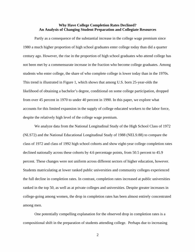
Partly as a consequence of the substantial increase in the college wage premium since

1980 a much higher proportion of high school graduates enter college today than did a quarter

century ago. However, the rise in the proportion of high school graduates who attend college has

not been met by a commensurate increase in the fraction who become college graduates. Among

students who enter college, the share of who complete college is lower today than in the 1970s.

This trend is illustrated in Figure 1, which shows that among U.S. born 25-year-olds the

likelihood of obtaining a bachelor’s degree, conditional on some college participation, dropped

from over 45 percent in 1970 to under 40 percent in 1990. In this paper, we explore what

accounts for this limited expansion in the supply of college educated workers to the labor force,

despite the relatively high level of the college wage premium.

We analyze data from the National Longitudinal Study of the High School Class of 1972

(NLS72) and the National Educational Longitudinal Study of 1988 (NELS:88) to compare the

class of 1972 and class of 1992 high school cohorts and show eight-year college completion rates

declined nationally across these cohorts by 4.6 percentage points, from 50.5 percent to 45.9

percent. These changes were not uniform across different sectors of higher education, however.

Students matriculating at lower ranked public universities and community colleges experienced

the full decline in completion rates. In contrast, completion rates increased at public universities

ranked in the top 50, as well as at private colleges and universities. Despite greater increases in

college-going among women, the drop in completion rates has been almost entirely concentrated

among men.

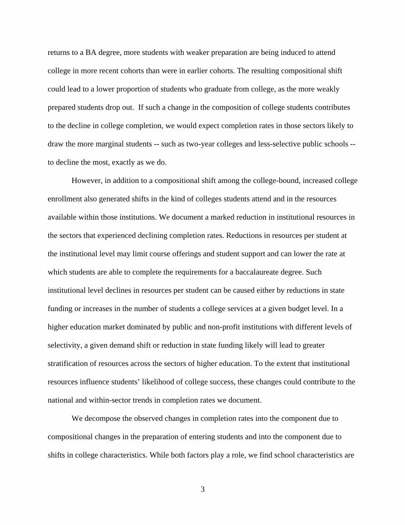
One potentially compelling explanation for the observed drop in completion rates is a

compositional shift in the preparation of students attending college. Perhaps due to increasing

3

returns to a BA degree, more students with weaker preparation are being induced to attend

college in more recent cohorts than were in earlier cohorts. The resulting compositional shift

could lead to a lower proportion of students who graduate from college, as the more weakly

prepared students drop out. If such a change in the composition of college students contributes

to the decline in college completion, we would expect completion rates in those sectors likely to

draw the more marginal students -- such as two-year colleges and less-selective public schools --

to decline the most, exactly as we do.

However, in addition to a compositional shift among the college-bound, increased college

enrollment also generated shifts in the kind of colleges students attend and in the resources

available within those institutions. We document a marked reduction in institutional resources in

the sectors that experienced declining completion rates. Reductions in resources per student at

the institutional level may limit course offerings and student support and can lower the rate at

which students are able to complete the requirements for a baccalaureate degree. Such

institutional level declines in resources per student can be caused either by reductions in state

funding or increases in the number of students a college services at a given budget level. In a

higher education market dominated by public and non-profit institutions with different levels of

selectivity, a given demand shift or reduction in state funding likely will lead to greater

stratification of resources across the sectors of higher education. To the extent that institutional

resources influence students’ likelihood of college success, these changes could contribute to the

national and within-sector trends in completion rates we document.

We decompose the observed changes in completion rates into the component due to

compositional changes in the preparation of entering students and into the component due to

shifts in college characteristics. While both factors play a role, we find school characteristics are

4

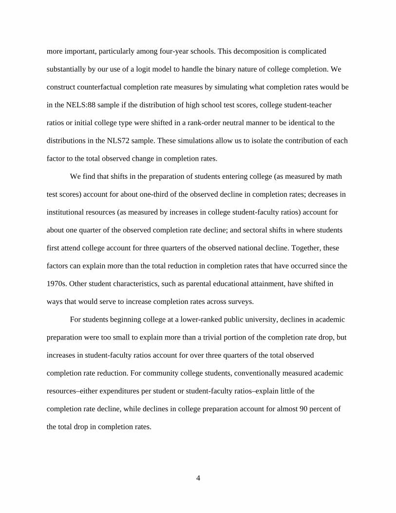
more important, particularly among four-year schools. This decomposition is complicated

substantially by our use of a logit model to handle the binary nature of college completion. We

construct counterfactual completion rate measures by simulating what completion rates would be

in the NELS:88 sample if the distribution of high school test scores, college student-teacher

ratios or initial college type were shifted in a rank-order neutral manner to be identical to the

distributions in the NLS72 sample. These simulations allow us to isolate the contribution of each

factor to the total observed change in completion rates.

We find that shifts in the preparation of students entering college (as measured by math

test scores) account for about one-third of the observed decline in completion rates; decreases in

institutional resources (as measured by increases in college student-faculty ratios) account for

about one quarter of the observed completion rate decline; and sectoral shifts in where students

first attend college account for three quarters of the observed national decline. Together, these

factors can explain more than the total reduction in completion rates that have occurred since the

1970s. Other student characteristics, such as parental educational attainment, have shifted in

ways that would serve to increase completion rates across surveys.

For students beginning college at a lower-ranked public university, declines in academic

preparation were too small to explain more than a trivial portion of the completion rate drop, but

increases in student-faculty ratios account for over three quarters of the total observed

completion rate reduction. For community college students, conventionally measured academic

resources–either expenditures per student or student-faculty ratios–explain little of the

completion rate decline, while declines in college preparation account for almost 90 percent of

the total drop in completion rates.

5

The key finding of this analysis is that the supply-side of higher education plays an

important role in explaining changes in student outcomes. The higher education literature has

focused on how student preparation for college translates into college success. Our analysis

suggests that, at least for changing completion rates, student preparation is only a partial

explanation; characteristics of the supply-side of the market have a substantial influence on

student success in college.

In Section I of this paper, we describe the data we use and show the changes in

completion rates found in the data, both nationally and across sectors of higher education. In

Section II, we outline a theoretical framework for understanding why these observed changes

have occurred and describe our empirical framework for distinguishing between these potential

explanations. In Section III, we present the results from our decomposition analysis, and in

Section IV we offer our conclusions.

I. Data and Descriptive Statistics

A. Measuring Completion Rates

The data for our analysis come from NLS72 and NELS:88. We use these datasets rather

than larger datasets with more cohorts of observation, such as the U.S. Census, because the

NLS72 and NELS:88 contain information on which college each student attended, the timing of

attendance, and graduation outcomes that are necessary to accurately measure cohort-specific

completion rates.1 These surveys draw from nationally representative cohorts of high school and

middle school students, respectively, and track the progress of students longitudinally through

1 Note that trends in college completion rates are inherently difficult to calculate. First, prior to the 1990s,

most national surveys asked about educational attainment in terms of completed years of schooling, where completing four years of college is only an imperfect proxy for BA degree attainment. Second, distinguishing immigrants from those born in the United States is important in time series analysis as the number of immigrants with at least a college degree has increased dramatically in the last 15 years.

6

collegiate and early employment experiences. We define the completion rate as the proportion of

students who attend college within two years of cohort high school graduation2 and obtain a BA

within eight years of cohort high school graduation.3

B. Trends in College Enrollment and Completion Rates

The longitudinal surveys show that college enrollment rates and college completion rates

have not moved in parallel in recent decades in the United States. Between the two cohorts there

was a substantial increase in college participation, which occurred against the background of

little appreciable change in high school graduation rates or measured secondary school

achievement.4

As illustrated in Table 1, the overall participation rate increased from 48.4 percent to 70.7

percent. Although the size of the high school graduation cohort was smaller in 1992 than in

1972, the increased attendance rate led to growth in the number of students attending college,

from 1.4 to 1.8 million. By gender, the increase is greater for women, rising from 46.5 percent to

73.5 percent, than it is for men, rising from 50.4 percent to 68.0 percent.

2 Cohort high school graduation is June 1972 for NLS72 respondents and June 1992 for NELS:88

respondents. See the Technical Appendix in Appendix A for detailed discussion of the NLS72 and NELS:88 datasets used in this analysis. Restricting the analysis to those who attend college within two years of cohort high school graduation has little effect on the results. In NLS72, 11.1 percent of college attendees delayed entry by more than two years, and in NELS:88, 8.8 percent delayed entry by more than two years. Changes in the timing of first entry thus cannot explain the shifts over time in completion rates between the two surveys.

3 Note that there may be some further closure in aggregate college completion rates measured with a longer lag from high school graduation. John Bound, Michael Lovenheim, and Sarah Turner (2007) show that while there has been a substantial elongation of time to degree that has occurred between these two surveys, much of this change is shifts within the eight-year window of observation; the proportion of eventual college degree recipients receiving their degrees within eight years does not appear to have changed appreciably. Using the 2003 National Survey of College Graduates, which allows us to examine year of degree by high school cohort, we find the share of eventual degree recipients finishing within eight years holds nearly constant between 0.83 and 0.85 for the high school classes of 1960 to 1979. Focusing on more recent cohorts (and, hence, observations with more truncation) we find that in the 1972 high school graduating cohort, 92.3 percent of those finishing within twelve years had finished in eight years, with a figure of 92.4 percent for the 1988 cohort.

4 Tabulations from the October Current Population Survey (CPS) show 81.0 percent of nineteen-year-olds in 1972 had a high school degree and, in 1992, 81.8 percent had a high school diploma. James J. Heckman and Paul A. Lafontaine (Forthcoming) use a variety of data sources and show relatively stable high school graduation rates over the time period of our analysis as well.

7

To capture the differentiation among collegiate experiences, we split post-secondary

institutions into five sectors, which are reflected in Table 1: non-top 50 public four-year schools,

top 50 public four-year schools, less selective private four-year schools, highly selective private

four-year schools, and community colleges.5 Table 1 illustrates that the overall increase in

college participation has not been divided evenly among different types of institutions in the U.S.

postsecondary market. The largest change over this time has been the 12.5 percentage point

increase in the likelihood of starting at a community college;6 these shifts were larger for men

than for women.

Overall, increases in the rate of college enrollment have been accompanied by decreases

in completion rates (Table 2). Similar to the enrollment shifts, these changes were not uniform

across sectors: the BA completion rate among those starting at public two-year institutions

slipped to 17.6 percent from 20.2 percent. Similarly, the completion rate fell by 4.9 percentage

points between the NLS72 and NELS:88 cohorts among students beginning college in public

non-top 50 institutions. In contrast, completion rates increased in the top 50 public schools as

well as in private schools. The divergence in completion rates by type of institution suggests that

national trends fail to record the stratification in outcomes that occurred both within the four-year

sector and between the four-year sector and community colleges since the 1970s. The erosion in

completion rates within the non-top 50 public sector suggests that the national trends are not

5 We employ the rankings assembled by U.S. News and World Report in 2005 to classify schools into one of the five divisions. The top 50 public schools are all public colleges and universities ranked in the top 50 in that year, and the highly selective private schools are composed of the top 65-ranked private universities and the top 50-ranked liberal arts colleges (plus the U.S. Armed Services Academies). These schools are listing in Appendix A. Other metrics, such as resources per student or selectivity in undergraduate admissions, give similar results. While these divisions are admittedly somewhat arbitrary, on the whole they capture the differences across the different types of post-secondary schools. The U.S. News rankings of institutions are highly correlated over time, and there are few changes across the large groupings we use to categorize schools. Thus, our use of the 2005 rankings when we are studying earlier periods will not affect our results.

6 All references to two-year schools and community colleges refer to public institutions only. We exclude private two-year schools as they often are professional schools with little emphasis on eventual BA completion. In the NLS72 cohort, 1.7 percent attended a private two-year school, and 1.1 percent of the NELS:88 sample attended such an institution.

8

being driven solely by the enrollment shift to community colleges, where completion rates are

lower and many students may not intend ultimately to earn a BA.

While including community college students in our aggregate measure magnifies the total

reduction in completion rates, we believe this inclusion is appropriate for two reasons. First,

although it is possible that some students enter community colleges for sub-baccalaureate

vocational training, the majority (69.9 percent) of community college entrants in the NELS:88

cohort intended to complete a BA.7 Secondly, because attendance at a community college

provides the important option to continue to the completion of a four-year degree, these students

are significant in the determination of cohort college completion rates.

Table 2 also contains completion rate changes across cohorts separately by gender. In

general, men’s completion rates declined substantially relative to women’s, with the rate for

males dropping by 8.5 percentage points and the rate for women declining a not statistically

significant 0.6 percentage points. Similar trends are apparent across sectors. For men attending

public non-top 50 universities and community colleges, completion rates dropped substantially.

For women, while completion rates fell slightly in the non-top 50 public and community college

sectors, rates rose dramatically in the top 50 public and private sectors.

C. Measuring Student Attributes

One of the major advantages of the NLS72 and NELS:88 data is the rich set of

background information available about respondents. The student attributes we use throughout

this analysis are high school math test percentile,8 father’s education level, mother’s education

7 Note that aspirations for degree completion among community college students who are recent high

school graduates are likely to be somewhat higher than measures for the overall population of community college students that includes a high fraction of older and non-traditional students. Our results are broadly consistent with Laanan Santos (2003), who employs the 1996 Freshman Survey from Cooperative Institutional Research Program (CIRP).

8 The math tests refer to the exams administered by the National Center for Education Statistics (NCES) that were given to all students in the longitudinal surveys in their senior year of high school. Because the tests in

9

level, real parental income levels, gender, and race. Our analysis uses math test percentiles as our

primary indicators of college preparation because, under reasonable assumptions, we are able to

compare these measures over time and among students attending different high schools. 9

Because there has been little change in the overall level of test scores on the nationally-

representative National Assessment of Educational Progress (NAEP) over our period of

observation, we argue that the academic preparation of high school graduates did not change

over our period of observation. Conditional on math test percentiles, we find other tests, such as

reading, have no predictive power for completion rates. Decomposition results with the inclusion

of reading test percentiles in the analysis are unchanged from those reported below, and we

therefore use only math test percentiles for parsimony in the empirical analysis.

Mother’s and father’s education is split into five levels: less than high school, high school

diploma (including a GED), some college, college graduate and any post-collegiate attainment.

For the measurement of family income, we are interested in assessing parents’ ability to finance

college, so the variable of interest is the real income level, not one’s place in the income

distribution. We align income in the two surveys using the Consumer Price Index (CPI) into 6

comparable income blocks representing responses to categorical questions about parental

income.

The NLS72 and NELS:88 datasets contain a significant amount of missing information

on test scores, parental education and parental income brought about by item non-response.

While a small share of observations is missing all of these variables (in NLS72 and NELS:88,

NLS72 and NELS:88 covered different subject matter, were of different lengths, and were graded on different scales, the scores are not directly comparable across surveys. We therefore assign each respondent a math test percentile, which is his percentile in the entire distribution of test-takers who graduated from high school.

9 This test score measure is used as a simple proxy for preparedness. Measures of high school performance such as high school GPA and class rank are other commonly used measures of preparation. We have chosen not to include GPA measures because we are concerned about difficulty in comparing this measure across high schools and the presence of grade inflation over time.

10

respectively, 0.5 percent and 0.6 percent have no information on any of these variables), a

substantial number of cases are missing either test scores, parental education or parental

income.10 We use multiple imputation methods (Donald B. Rubin, 1987) on the sample of all

high school graduates to impute missing values using other observable characteristics of each

individual.11 The Technical Appendix (available online) to this paper in Appendix A contains

detailed information on the construction of our data set.

Table 3 presents the changes in background characteristics and academic preparation of

college attendees and graduates across the NLS72 and NELS:88 surveys. Notably, there was a

sizeable shift in the proportion of students entering college from lower on the high school test

score distribution. Average math test percentiles among those enrolling in college dropped from

62.5 to 58.0 across cohorts, and the percent of college attendees from the highest math test

quartile dropped from 40.7 to 32.8, while the percent from the lowest math test quartile increased

from 11.2 to 15.6. However, these declines occurred only in the two-year sector; math test

percentiles remained constant or increased in all four year sectors across the two surveys. This

fact foreshadows a key finding of this paper: that changing student college preparation, as

measured by math test percentiles, cannot account for the decline in completion rates in the

public non-top 50 sector.

10 For example, in NLS72, 40.5 percent of those who enroll in college and 40.8 percent of those receiving a

BA within eight years of cohort high school graduation are missing information on at least one of these background characteristics. These percents are 42.5 and 37.5, respectively, in NELS:88. Because the data are not missing completely at random, case-wise deletion of observations with missing variables will bias the unconditional sample means of completion rates.

11 Under the assumption that the data are missing conditionally at random, multiple imputation is a general and statistically valid method for dealing with missing data (Rubin, 1987; Little, 1982). The relative merits of various approaches for dealing with missing data have been widely discussed (e.g. Little and Rubin, 2002; Schafer, 1997). See the Technical Appendix in Appendix A for complete details of the imputation procedure. Because the surveys contain good supplementary predictor variables, such as high school GPA, standardized test scores from earlier survey waves, and parental income reports, we are able to use a great deal of information about each respondent to impute ranges of missing data points.

11

Figure 2 shows the likelihood of college entry and college completion for high school

graduates, as well as the completion rate conditional on college entry. The figure clearly

indicates that the likelihood of attending college rose across the board. In 1972, there were many

high school graduates who appear to have been well qualified to attend college but who did not

enroll. By 1992, this was a rarer phenomenon. At the same time, the figure makes clear that the

greatest enrollment shifts occurred for those that appear less well prepared, and those with

relatively low academic achievement were unlikely to complete the BA degree in either cohort.

As a result, the average math test percentile actually rises among BA recipients across the two

cohorts, from 70.7 to 71.7. In the bottom quartile of the test score distribution, the likelihood of

attending college increases from 21.7 percent to 44.0 percent, which is consistent with a larger

percentage of less-prepared students attending college in the later cohort in order to take

advantage of the rising returns to education. However, among this group, only 5.6 percent in the

initial period of observation receive a BA, and this percent falls yet further to 5.0 for the later

cohort. Focusing on college attendees, the likelihood of completing a BA declined from 25.8

percent to 11.4 percent across cohorts for those in the bottom quartile of math test scores. The

strong link between our measure of pre-collegiate achievement and the likelihood of college

completion shown in Figure 2 suggests that changes in the distribution of preparation among

college entrants is a potentially important factor in understanding the change in the aggregate

college completion rate.

The gender differences in college completion shown in Table 2 correspond to a dramatic

decline in the skill gap between men and women across cohorts, as measured by pre-collegiate

math test percentiles. Figure 3 presents cumulative distributions of math test percentiles for the

full sample of college attendees and separately by college sector. Overall, the distribution of

12

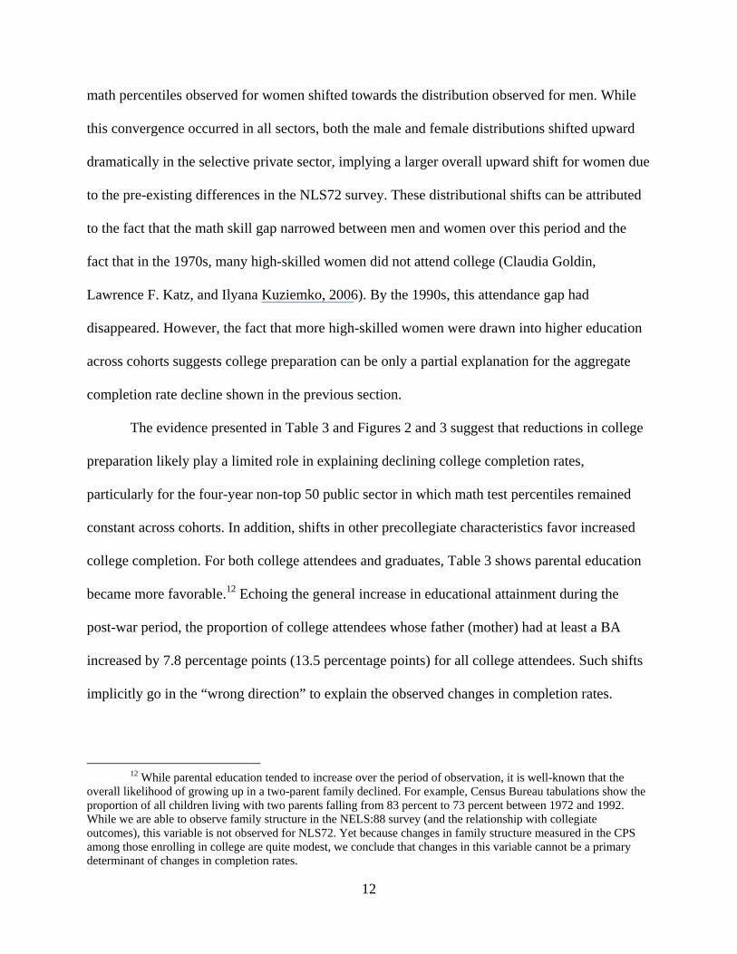
math percentiles observed for women shifted towards the distribution observed for men. While

this convergence occurred in all sectors, both the male and female distributions shifted upward

dramatically in the selective private sector, implying a larger overall upward shift for women due

to the pre-existing differences in the NLS72 survey. These distributional shifts can be attributed

to the fact that the math skill gap narrowed between men and women over this period and the

fact that in the 1970s, many high-skilled women did not attend college (Claudia Goldin,

Lawrence F. Katz, and Ilyana Kuziemko, 2006). By the 1990s, this attendance gap had

disappeared. However, the fact that more high-skilled women were drawn into higher education

across cohorts suggests college preparation can be only a partial explanation for the aggregate

completion rate decline shown in the previous section.

The evidence presented in Table 3 and Figures 2 and 3 suggest that reductions in college

preparation likely play a limited role in explaining declining college completion rates,

particularly for the four-year non-top 50 public sector in which math test percentiles remained

constant across cohorts. In addition, shifts in other precollegiate characteristics favor increased

college completion. For both college attendees and graduates, Table 3 shows parental education

became more favorable.12 Echoing the general increase in educational attainment during the

post-war period, the proportion of college attendees whose father (mother) had at least a BA

increased by 7.8 percentage points (13.5 percentage points) for all college attendees. Such shifts

implicitly go in the “wrong direction” to explain the observed changes in completion rates.

12 While parental education tended to increase over the period of observation, it is well-known that the

overall likelihood of growing up in a two-parent family declined. For example, Census Bureau tabulations show the proportion of all children living with two parents falling from 83 percent to 73 percent between 1972 and 1992. While we are able to observe family structure in the NELS:88 survey (and the relationship with collegiate outcomes), this variable is not observed for NLS72. Yet because changes in family structure measured in the CPS among those enrolling in college are quite modest, we conclude that changes in this variable cannot be a primary determinant of changes in completion rates.

13

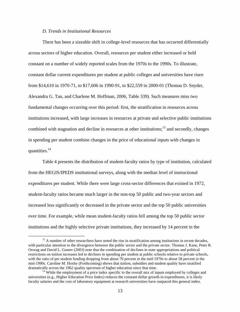
D. Trends in Institutional Resources

There has been a sizeable shift in college-level resources that has occurred differentially

across sectors of higher education. Overall, resources per student either increased or held

constant on a number of widely reported scales from the 1970s to the 1990s. To illustrate,

constant dollar current expenditures per student at public colleges and universities have risen

from $14,610 in 1970-71, to $17,606 in 1990-91, to $22,559 in 2000-01 (Thomas D. Snyder,

Alexandra G. Tan, and Charlene M. Hoffman, 2006, Table 339). Such measures miss two

fundamental changes occurring over this period: first, the stratification in resources across

institutions increased, with large increases in resources at private and selective public institutions

combined with stagnation and decline in resources at other institutions;13 and secondly, changes

in spending per student combine changes in the price of educational inputs with changes in

quantities.14

Table 4 presents the distribution of student-faculty ratios by type of institution, calculated

from the HEGIS/IPEDS institutional surveys, along with the median level of instructional

expenditures per student. While there were large cross-sector differences that existed in 1972,

student-faculty ratios became much larger in the non-top 50 public and two-year sectors and

increased less significantly or decreased in the private sector and the top 50 public universities

over time. For example, while mean student-faculty ratios fell among the top 50 public sector

institutions and the highly selective private institutions, they increased by 14 percent in the

13 A number of other researchers have noted the rise in stratification among institutions in recent decades,

with particular attention to the divergence between the public sector and the private sector. Thomas J. Kane, Peter R. Orszag and David L. Gunter (2003) note that the combination of declines in state appropriations and political restrictions on tuition increases led to declines in spending per student at public schools relative to private schools, with the ratio of per student funding dropping from about 70 percent in the mid-1970s to about 58 percent in the mid-1990s. Caroline M. Hoxby (Forthcoming) shows that tuition, subsidies and student quality have stratified dramatically across the 1962 quality spectrum of higher education since that time.

14 While the employment of a price index specific to the overall mix of inputs employed by colleges and universities (e.g., Higher Education Price Index) reduces the constant dollar growth in expenditures, it is likely faculty salaries and the cost of laboratory equipment at research universities have outpaced this general index.

14

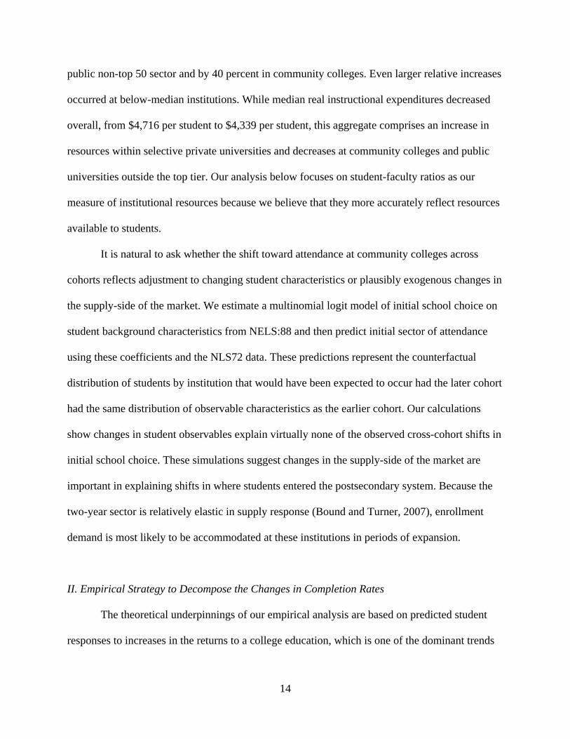
public non-top 50 sector and by 40 percent in community colleges. Even larger relative increases

occurred at below-median institutions. While median real instructional expenditures decreased

overall, from $4,716 per student to $4,339 per student, this aggregate comprises an increase in

resources within selective private universities and decreases at community colleges and public

universities outside the top tier. Our analysis below focuses on student-faculty ratios as our

measure of institutional resources because we believe that they more accurately reflect resources

available to students.

It is natural to ask whether the shift toward attendance at community colleges across

cohorts reflects adjustment to changing student characteristics or plausibly exogenous changes in

the supply-side of the market. We estimate a multinomial logit model of initial school choice on

student background characteristics from NELS:88 and then predict initial sector of attendance

using these coefficients and the NLS72 data. These predictions represent the counterfactual

distribution of students by institution that would have been expected to occur had the later cohort

had the same distribution of observable characteristics as the earlier cohort. Our calculations

show changes in student observables explain virtually none of the observed cross-cohort shifts in

initial school choice. These simulations suggest changes in the supply-side of the market are

important in explaining shifts in where students entered the postsecondary system. Because the

two-year sector is relatively elastic in supply response (Bound and Turner, 2007), enrollment

demand is most likely to be accommodated at these institutions in periods of expansion.

II. Empirical Strategy to Decompose the Changes in Completion Rates

The theoretical underpinnings of our empirical analysis are based on predicted student

responses to increases in the returns to a college education, which is one of the dominant trends

15

in higher education over the past 30 years. As the returns to a college degree increase, more

students are induced to attend college and more of the students who already would have attended

college will complete in order to realize the return on their investment. Thus, holding student

skills and college quality constant, an increase in the return to college should increase the

likelihood of college completion. However, many of the newer students induced to attend college

will be less prepared for collegiate success and these marginal students are likely to have a lower

probability of completing college than the inframarginal students. These two shifts have opposite

effects on completion rates. Which effect will dominate is an empirical question.

Changes in the supply-side of the market, including which sector of higher education

college students attend and the resources per student at these colleges, also can affect collegiate

attainment. Increasing college attendance itself may further change the resources to which

students are exposed while enrolled. Because the higher education market is dominated by public

colleges and universities with budget systems that do not adjust fully to demand increases, higher

enrollment leads to a reduction in resources per student, with increased scarcity (selectivity) at

those institutions that are the most resource-intensive. Nevertheless, even in the presence of

reductions in expected resources per student and a reduced likelihood of attending a top-tier

institution resulting from a general demand increase for postsecondary education, uncertainty

about actual collegiate resources and likelihood of collegiate success can induce students to

enroll in an institution with low resources in order to take advantage of high potential returns

(i.e., the option value of schooling15), only to find out that it is difficult to enroll in required

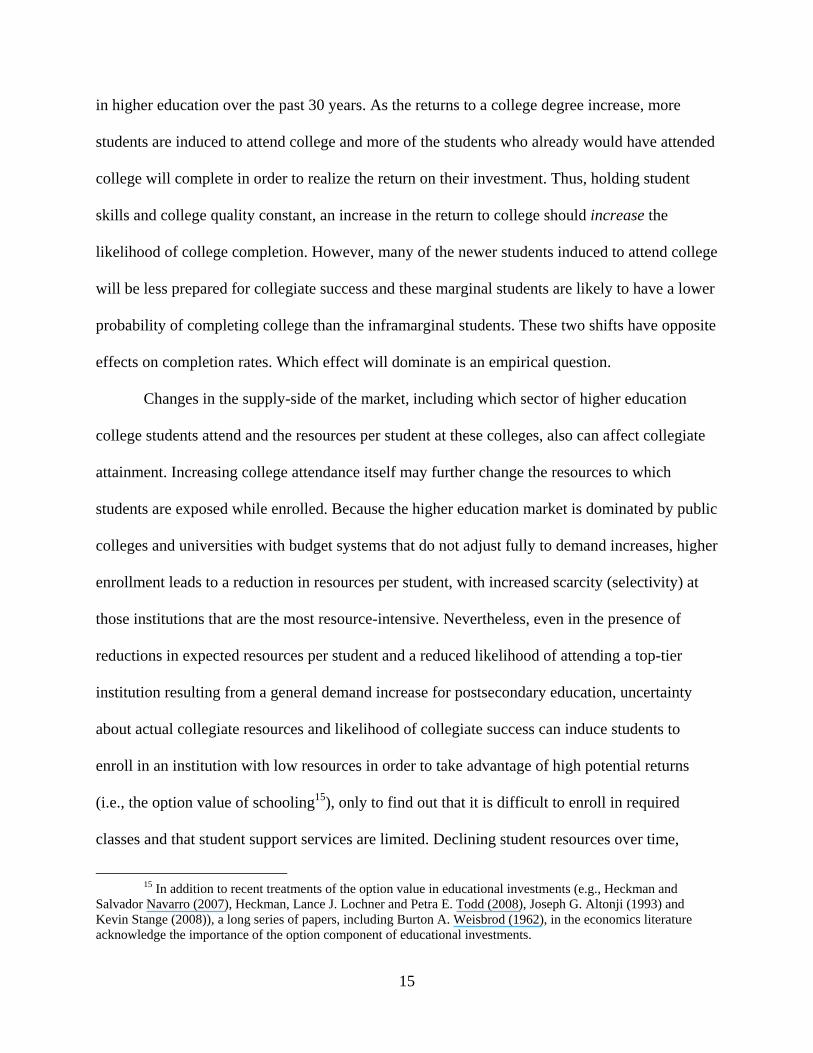
classes and that student support services are limited. Declining student resources over time,

15 In addition to recent treatments of the option value in educational investments (e.g., Heckman and

Salvador Navarro (2007), Heckman, Lance J. Lochner and Petra E. Todd (2008), Joseph G. Altonji (1993) and Kevin Stange (2008)), a long series of papers, including Burton A. Weisbrod (1962), in the economics literature acknowledge the importance of the option component of educational investments.

16

particularly in non-top 50 public universities and community colleges, therefore may play a role

in explaining the trends in completion rates we observe in the data.

It is important to emphasize that the demand-side and supply-side explanations described

above are not mutually exclusive: less-prepared students sort into the most elastic sectors of

higher education, which tend to have the fewest resources. In essence, increased demand for

college crowds more students (and more less-prepared students) into community colleges and

non-top 50 public universities. Demand increases therefore not only lower the resources per

student at these institutions, but cause higher dispersion in resources across the sectors of higher

education. The implication of this sorting process is that one should observe the largest declines

in completion rates in the most elastic sectors, which is indeed the pattern prevalent in the data.

Because changes in student preparation for college and institutional resources are closely

linked through the returns to education and the college admissions system, it is not clear from

examining the aggregate data how important individual demand-side or supply-side factors are in

explaining changing college completion rates. Our empirical objective in the paper is to

disentangle the individual contribution of these factors; we seek to decompose the total change

into the part due to shifts in student preparation and the part due to college-level factors.

In order to isolate the independent effects of student preparation and college resource changes on

changes in completion rates, we run logit models of the probability of completion on student

math test percentiles, collegiate student-faculty ratios, student demographic characteristics and

initial college-type fixed effects.

The central difficulty in undertaking the proposed decompositions stems from the non-

linearity of the logistic function. In a linear framework, the decomposition is straightforward: the

change in the mean of an explanatory variable multiplied by the estimated coefficient on that

17

variable from the outcome regression represents the partial effect that the change in this

characteristic has on the total change in the outcome. For example, if one estimated our

completion equation using a linear probability model, the effect of changes in any observable (xj)

on the observed change in completion rates could be calculated simply by multiplying the

estimated partial effect of xj on completion rates by the change in the mean of xj across surveys.

In a non-linear model, such as a logit, the exercise becomes both conceptually and

computationally more difficult because the estimated partial effects vary across the sample. For

individuals who are estimated to be either very likely or very unlikely to finish college, changes

in xj will have little effect on the changes in the probability of completion. On the other hand, for

individuals whom our estimates suggest have a roughly fifty percent chance of finishing college,

changes in the observables will have a potentially large effect on the estimated likelihood of

college completion. We therefore cannot simply multiply the estimated marginal effect by the

difference in means across samples, as the simulated effects of a discrete change in an

explanatory variable will depend on what part of the distribution shifted.

Simulating the change in all of the explanatory variables is straightforward; one method

is to use estimates from the NELS:88 data to simulate predicted probabilities using the NLS72

data. The difference between the average of these predicted probabilities and the sample fraction

that complete college in the NELS:88 data represents an estimate of the effect of compositional

changes of all our observables on completion rates.16 Note that non-parametric reweighting using

the characteristics of students from the NLS72 survey would produce a nearly identical

counterfactual completion rate in which the proportion of students with a given characteristic or

16 Starting with estimates of completion generated from the NLS72 baseline produces parallel results.

18

a given set of characteristics has not changed between the two surveys.17 We employ the former

method to simulate the effect of a change in all observables on the change in completion rates,

but we obtain similar results when we use non-parametric reweighting techniques.

Beyond measuring the total effect of compositional changes, we want to estimate the

effect of changes in individual explanatory variables. To this end, we want to predict the

completion rate under the counterfactual assumption that test scores followed the distribution of

the early cohort while other covariates maintained the later distribution. Sergio Firpo, Fortin, and

Lemieux (2007) note the general challenge in dividing the composition effect into the role of

each covariate for distributional measures beyond the mean. Focused on distributional measures

in the context of the structure of earnings, the authors develop a general method for doing this

decomposition using influence functions. In our context of a dichotomous dependent variable,

we pursue an approach focused on estimation of the counterfactual for any variable using a

matching estimator.

It will be easiest to explain our approach in the context of a specific example. We are

interested in using our estimates to simulate the effect that a change in the distribution of college

preparation, proxied by the change in math test percentiles among college goers, had on

completion rates. To do this simulation, we construct counterfactual variables by assigning to

each observation in the NELS:88 sample a math test percentile from the NLS72 sample that

corresponds to the same relative rank: the individual with the highest percentile score in

NELS:88 is assigned the top value from NLS72, the second-ranked in each survey are matched,

and so on (with ties broken randomly). Done without replacement, this matching algorithm

17 Re-weighting estimators have a long history in statistics dating back at least to the work of Daniel G.

Horvitz and David J. Thompson (1952) and have become increasingly popular in economics (see, for example, John DiNardo, Nicole M. Fortin and Thomas Lemieux, 1996; Heckman, Hidehiko Ichimura, and Todd, 1997 and 1998; and Robert Barsky, Bound, Kerwin Charles and Joseph Lupton, 2002).

19

reproduces the NLS72 math test percentile distribution in the NELS:88 sample, holding relative

ranking constant across the surveys. This method ensures we are not randomly assigning high

(low) math test values to individuals who would be predicted to have low (high) math test scores

based on the other characteristics we observe about respondents. We then use the parameters

from our estimated logit model of completion on the NELS:88 sample and calculate

counterfactual completion rates in which math tests scores have changed in a rank-neutral

manner but other characteristic have remained the same. While the above example focuses on

math test distribution changes, it is straightforward to use this methodology to generate

counterfactual completion rates for a shift in any of our independent variables.18

The validity of our counterfactual calculations (e.g., what would the college completion

rate for those attending college in the 1990s have been had they been as academically prepared

for college as those who attended in the 1970s?) depends crucially on the cross-sectional

association between background characteristics and college outcomes reflecting a causal

relationship not seriously influenced by confounding factors.19 For example, we simulate

completion rates under a counterfactual distribution of test scores. For this simulation to

accurately represent the counterfactual, it must be the case that the cross-sectional relationship

between test scores and the likelihood of college completion reflects the impact of pre-collegiate

academic preparation on this outcome. Regardless of whether the simulation calculation

produces the “true” counterfactual, the results present a clear accounting framework for

assessing the descriptive impact of the change in the composition of students and the institutions

they attend on collegiate attainment.

18 When we construct counterfactual completion rates for student-faculty ratios, we do not assign a

counterfactual value to NELS:88 respondents with missing student-faculty ratios. This methodology allows us to match student-faculty ratio distributions among those with observed student-faculty ratios in both surveys.

19 Firpo, Fortin, and Lemieux (2007) make the same point.

20

A related identification issue associated with our decomposition analysis is that math test

percentiles and student-faculty ratios must be accurate proxies of student preparation and

institutional resources, respectively. A particular concern is that both test scores and student-

faculty measures are imperfect proxies for the constructs in which we are interested. While the

general effect of such errors in measurement is to bias downward the effects estimated in the

simulations, we are unable to assess the relative adequacy of these measures. Nevertheless, in the

case where the distribution of test scores does not change across cohorts while the distribution of

resources changes markedly, we can be confident that changes in preparation are not central in

the explanation. Moreover, within sector, the correlation between test scores and student-faculty

measures is low. This supports the interpretation that institutional resource effects are not simply

reflecting the effects of unmeasured “ability” generated by the correlation with the residual part

of academic preparation not captured by our math test measure. To further address this concern,

we run state-level regressions of college completion rates from the U.S. Census on the size of the

college-age population. As argued by Bound and Turner (2007), the college-age population

serves as an instrument for collegiate resources because demand shocks are unlikely to be fully

accounted for by the public state budgeting system. We use this instrument in order to determine

whether completion rates within states vary systematically with these demand shocks in order to

give further evidence of the importance of collegiate resources in determining college

completion rates.

21

III. Empirical Analysis of Changes in Completion Rates

A. Results from Completion Logits

The coefficients from the completion logits estimated for the NLS72 sample and the

NELS:88 sample are shown in Table 5 for the full sample and separately by initial school type.20

Overall, the coefficients shown in Table 5 have the expected signs: higher student-faculty ratios

and lower math test percentiles lower the likelihood of completion.21 This pattern is evident

within sectors as well. We find consistent evidence that increases in student-faculty ratios reduce

completion, both for the full sample and within sectors. However, similar to Stange (2009), we

find little evidence that measured collegiate resources affect the likelihood of completion in the

community college sector. This result could be due to the fact that within-sector variation in

institutional resources matters little in determining the likelihood of obtaining a BA for

community college students. More plausibly, perhaps, our resource measures do a particularly

poor job measuring resources devoted to the two-year college student potentially bound for a

four-year school. Some of the most resource-intensive programs at community colleges are

likely to be vocational programs of short duration. In addition, student-faculty ratios are a

noisier resource measure in community colleges than in the other sectors of higher education

because of the greater incidence of students attending less than full-time and faculty employed

on an adjunct basis.

20 In addition to the variables discussed in Section I, we include an indicator variable for whether the

respondent has no information on student-faculty ratios and an interaction between this indicator and math percentiles. In both NLS72 and NELS:88, 10.8 percent have missing student-faculty ratios. These data are missing either because the student’s first listed institution could not be matched with an institution in the HEGIS/IPEDS data or because the matched institution had missing HEGIS/IPEDS data. Rather than impute these ratios with very limited information, we include a dummy variable indicating missing status and allow the effect of missing institutional data to vary with math percentiles.

21 Similarly, Audrey Light and Wayne Strayer (2000) find evidence using the National Longitudinal Survey of Youth that both college quality and student ability affect the likelihood of college completion.

22

The initial school type indicators in the first two columns of Table 5 show that even

conditional on student-faculty ratios, there is a significantly higher likelihood of completion at

top 50 public and selective private schools and a significantly lower likelihood of completion at

community colleges.22 These results suggest there are unobserved aspects of college quality

across sectors not being proxied for by our institutional resource measure that are important in

explaining college completion.

B. Simulation Results for the Full Sample

Results from the decomposition analysis are shown in Table 6.23 The observed cohort

completion rates are presented in the first two rows, followed by the difference in the third row,

and the difference between the observed NELS:88 completion rate and the counterfactual

completion rate calculated using NELS:88 completion logit coefficients and all observables from

the 1972 cohort are shown in the fourth row. Overall, the covariates in our analysis explain the

entire decline in the completion rate.

In order to distinguish the effects of changes in variables like college preparation from

the effects of changes in supply-side variables like student-faculty ratios, we use the

decomposition methodology discussed in Section II. The subsequent rows of Table 6 show the

predicted change in completion rates based on these univariate simulations. For the Change Due

to Math Test Percentiles, we calculate the difference between the observed NELS:88 completion

rate and the simulated completion rate that would have prevailed if the observations in NELS:88

22 Researchers consistently have found college students starting at two-year schools are less likely to

complete the BA than their peers beginning at four-year schools. C. Lockwood Reynolds (2007) and Darwin W. Miller (2007) use matching estimators to approach this question, while earlier work uses regression techniques to adjust for observable differences between those starting at two and four-year schools (Cecilia Rouse, 1995; Duane E. Leigh and Andrew M. Gill, 2003; Arturo Gonzales, Michael J. Hilmer, and Jonathon Sandy, 2006).

23 Appendix B shows decompositions performed by multiplying either the average marginal effects from our logit models or the coefficients from a linear probability model on a given variable by the change in the mean value of the variable across surveys. In the former case, this amounts to the assumption that variable shifts were constant across the population, while in the later it amounts to the standard Blinder-Oaxaca decomposition. In both cases the results are qualitatively similar to those presented in Tables 6 and 7.

23

were to possess the same math test percentile distribution as the NLS72 cohort, holding all other

covariates constant. This simulation leads to a completion rate 1.6 percentage points higher than

the observed completion rate in the NELS:88 sample. At the same time, shifting other individual

characteristics (primarily parents’ education) back to their 1972 levels would lower completion

rates by a comparable amount. Conducting the same exercise for student-faculty ratios produces

a completion rate 1.1 percentage points higher than the observed NELS:88 completion rates,

while changing just institutional type produces a completion rate 3.5 percentage points higher

than observed. These results underscore the importance of supply-side factors in explaining

completion rate declines; shifts in where students enter the postsecondary system and changes in

student-faculty ratios together explain the entire observed decline in completion rates across

surveys. If we did not account for other student background characteristics shifting in ways that

would suggest an increase in completion rates, observed declines in student preparation and

supply-side factors would slightly over-explain the total observed decline.

C. Simulation Results by Initial School Type

Results from our decomposition analysis by initial school type also are shown in Table 6.

For students beginning college at non-top 50 public universities, the changes in math test

percentiles explain none of the observed completion rate decline. This result occurs despite the

fact that we find a sizeable positive effect of math tests on completion in this sector, as shown in

Table 5. However, as Figure 3 illustrates, the math test percentiles of incoming students at non-

top 50 public institutions have changed negligibly across surveys. Student preparation for

college, as measured by math test percentiles, has not changed enough to explain the completion

24

rate decline for non-top 50 ranked public university students.24 Instead, we find that the large

increase in student-faculty ratios reported in Table 4 can explain 81.6 percent of the total

observed drop in completion rates. At least for students in the non-top 50 public sector, supply-

side shifts are the dominant explanation for why completion rates have declined across surveys.

For students at community colleges, variation in student-faculty ratios has little

explanatory power, while observed declines in student preparation are notable. Reductions in the

math test percentile of incoming students can explain 88 percent of the 2.5 percentage point

decline in this sector. These results are consistent with the dramatic expansion of the community

college sector across cohorts and the fact that the less prepared students induced to attend college

in the later cohort are predominantly entering the postsecondary system through community

colleges.

At private universities and the top-tier public universities, the results are quite different.

Neither observable student characteristics nor institutional resource measures are particularly

powerful in explaining the quite prominent increases in college completion rates. This result is

not surprising–as discussed in Section II, increasing returns to education should raise completion

rates unless they are coupled with resource declines or increases in attendance among less

academically prepared students, neither of which occurred in these sectors.

D. Simulation Results by Gender

One of the striking results shown in Table 2 is the large difference in completion rate

changes across genders. Our estimates show a cohort effect in college completion for women,

with women in the later cohort completing college at much higher rates than their peers from the

earlier cohort in most sectors of higher education. A compelling and plausible explanation for

24 The fact that the math test percentile distribution changed negligibly in the non-top 50 public sector

suggests peer effects cannot explain the decline in completion rates in this sector because the composition of peers has remained relatively constant.

25

this shift is that labor market opportunities and the associated returns to college completion for

women changed over this period, with women in the later cohort much more likely to expect

extended labor force participation (Goldin, Katz, and Kuziemko, 2006). These labor market

changes are powerful demand-side factors affecting college completion rates.

Table 7 shows results from our decomposition analysis done separately by gender, using

the same logit coefficients as in Table 6 but generating within-gender counterfactual variable

distributions. These decompositions allow us to account separately for the importance of the

differences in the change in college preparation across genders and the differences between men

and women in how they sort into the sectors of higher education across cohorts. Furthermore,

because most of the decline in completion rates has been among men, it is important to

determine whether we can explain the decline among the more affected group. The results for

men, shown in Panel A, are similar to those in Table 6: while declines in math test percentiles

can explain about a quarter of the observed completion rate drop, it is predominantly the shift

across institutions combined with higher student-faculty ratios that are responsible for the

aggregate decline. Taken together, these two supply-side factors explain about 55 percent of the

completion rate drop for men, and our demand-side and supply-side factors together explain

about 80 percent. For the public non-top 50 sample, these factors can account for 43.8 percent of

the 9.6 percentage point decline, with student-faculty ratio increases acting as the driving force

behind these results. In the community college sector, it is predominantly the decline in math test

percentiles that can explain the overall completion rate drop, accounting for 69 percent of the

observed reduction in completion. Overall, we can explain 82 percent of the total completion rate

decline with our demand and supply side factors in this sector.

26

For women, as shown in Panel B of Table 7, the total effect of supply-side factors and

academic preparation is to overpredict the observed completion rate decline in the full sample as

well as in the non-top 50 public and community college sectors. In the public top 50 and private

sectors, women saw an increase in completion rates, but none of this increase is predicted by test

percentile and student-faculty ratio changes. Particularly at top-tier institutions, the collegiate

attainment of women conditional on measured academic achievement improved markedly

between cohorts.

Overall, the closing of the gender gap in college preparation between men and women

and the increasing likelihood that men and women attend similar colleges with similar resources

explains some of the gender difference in the change in completion rates. However, as implied

by the dramatic change in the coefficient on the male dummy in our completion rate logits (see

Table 5), most of the relative change is not explained by any of the explanatory variables in our

models. Changes in women’s expectations about the future potentially explains this residual

(Goldin, Katz and Kuziemko, 2006).

The increased participation of women in higher education between the 1972 and 1992

cohorts plausibly served to exacerbate supply constraints in the higher education market,

particularly in the four-year sector. If not for the disproportionate increase in the enrollment of

women, we expect that the distribution of men by type of initial enrollment would have reflected

greater representation at four-year institutions with relatively high completion rates and lower

enrollment at community colleges, as the four year sector is much less enrollment-elastic than

the two-year sector. To frame this idea, we use the numbers in Tables 1 and 2 to calculate what

the male completion rate would have been for the 1992 cohort had the overall enrollment shares

remained constant at their 1992 levels (column iv of Table 1), but had the gender ratios within

27

each category stayed at their 1972 levels. This simulation serves to increase the share of men

attending private colleges, in general, and selective private colleges, in particular. Holding sector

completion rates constant, we calculate that male completion rates for the 1992 cohort would

have been three percent higher under this alternative regime. Thus, relatively inelastic supply in

the most resource-intensive sectors of higher education served to generate crowd-out in the

distribution of enrollment choices of men, which magnified the decline in completion rates for

this group.

E. State-Level Evidence of the Effect of Collegiate Resources on College Completion

Since student-faculty ratios and high school math test percentiles may be imperfect

proxies for institutional resources and college preparation, respectively, we present supplemental

evidence on the link between changes in collegiate resources and changes in completion rates.

Because states are the governmental level of control for public universities, we exploit within-

state changes in the college-age population that generate exogenous variation in the level of

public higher education subsidies per student. Absence of full adjustment of public subsidies to

student demand shocks means that relatively large cohorts face diluted resources per student at

state-run institutions in what Bound and Turner (2007) describe as “cohort crowding.”

Using data from the 1940-1975 birth cohorts in the 2000 U.S. Census, we regress the log

of the state and birth cohort share of the population with at least some college attaining a BA

degree on log birth cohort size, including state and year fixed effects. The estimated coefficient

on log cohort size provides a reduced form estimate of the elasticity of college completion with

respect to cohort size; the basic approach parallels Bound and Turner (2007), though is

distinguished in the focus on completion relative to college attendance.

28

Our findings, presented in Table 8, show within-state increases in cohort size of ten

percent lead to declines in the share of BA recipients among those starting college of between

1.12 percent and 1.85 percent. The separate outcomes for men and women, shown in the final

two rows of Table 8, are similar in magnitude, though slightly more pronounced for men than for

women. Our results support the hypothesis that increases in the number of students attempting to

enroll in colleges and universities, particularly in public institutions, reduce both the rate of

college entry and the rate of completion conditional on college entry. Overall, the results using

the Census data provide further evidence of the empirical relevance of supply-side constraints in

determining completion rates.25 Taken together with the results from the logit simulations, these

estimates suggest that incomplete institutional adjustments to growth in the number of students

pursuing a college degree may foster increased stratification, with an increasingly smaller

portion of the student body receiving an increasingly larger fraction of the resources.

IV. Conclusion

Focusing on the inter-cohort comparison of college completion rates between the NLS72

(the high school class of 1972) and NELS:88 (the high school class of 1992) cohorts, we find

that declines in pre-collegiate preparation and changes in the distribution of supply-side options

in the higher education market–reflecting both institutional type and resources within

institutions–explain the substantial decline in college completion rates, particularly among men.

25 An alternative explanation is that changes in the demand for college may be reduced among relatively

large cohorts if college preparation is also linked to cohort size. Two related concerns surface. First, relatively large cohorts may be distinguished by adverse demographic or economic shocks that have direct effects on collegiate attainment. For example, if big cohorts are distinguished by low parental education or large family size, such “compositional effects” might account for reduced college completion rather than crowding out on the supply side of the market. Secondly, membership in a relatively large birth cohort may dilute educational resources at the elementary and secondary levels, which would also reduce college preparedness. Bound and Turner (2007) present evidence that neither of these effects is likely to account for much of the association between cohort size and college completion rates. In particular, using Census data, they found, at best, only a modest association between cohort size and the demographic composition of the college age population. They also found only a very modest effect of cohort size on the college preparedness of high school graduates.

29

By examining the type of college at which individuals begin their postsecondary careers, we

show the decrease in degree completion is largely concentrated among students beginning at

non-top 50 public universities and two-year colleges. As such, the progression from college

enrollment to BA receipt over the last three decades has become much more stratified as the

differences in resources per student have grown both between sectors and within sectors.

We find increased enrollment among students from lower in the pre-collegiate math test

score distribution, which is occurring solely at two-year schools, can explain about 33 percent of

the overall drop in college completion rates. The drop in completion rates has not occurred

equally across gender groups–we find large decreases among males but not females. That the

college enrollment rate has increased more for women than for men, yet declines in college

completion have been smaller for women than men, suggests changes in completion rates cannot

be due solely to increases in enrollment by marginal students.

Our analysis focuses on the supply-side of higher education, which has not received

much attention in previous literature. Changes in resources per student, as measured by student-

faculty ratios at the institution where a student begins college, account for about 1/4 of the

observed aggregate decline in the college completion rate. Similarly, we find the shift in the

distribution of students’ initial college type, largely the shift toward community colleges,

explains roughly 3/4 of the observed decrease in completion rates.

We argue one reason for the importance of the initial institution type in explaining

reductions in completion probabilities is the increased stratification across sectors that has

occurred over the time period covered by our analysis. This increased stratification in resources

is likely a response to demand shocks combined with increased market integration that has

produced more differentiation, leading to declines in resources per students outside the selective

30

public and private universities where rationing occurs through selective admissions. Thus, while

“access” or initial college enrollment has increased dramatically over the past three decades,

many of the new students drawn to higher education (likely to take advantage of the increased

returns to a BA) are attending institutions with fewer resources and are not graduating. The

mechanisms by which this is occurring, however, deserve more attention in future research.

That decreases in college completion rates are concentrated among students attending

public colleges and universities outside the most selective few suggests a need for more attention

to the budgets of these institutions from state appropriations and tuition revenues. These

institutions may face tradeoffs between fulfilling an open access mission by increasing

enrollment at low tuition with reduced resources per student and either raising tuition, which

may reduce “access,” or limiting enrollment in order to increase resources per student. In

drawing attention to changes in the composition of students as well as the supply-side of the

market for higher education as explanations for declining completion rates, this analysis suggests

that improving the understanding of the factors determining the level of collegiate attainment has

substantial implications for the expected trend in the college wage premium and long-run

economic growth.

Page 31

References

Altonji, Joseph G. 1993. “The Demand for and Return to Education When Education Outcomes are Uncertain.” Journal of Labor Economics, 11(1):48-83. Barsky, Robert, John Bound, Kerwin Charles, and Joseph Lupton. 2002. “Accounting for the Black-White Wealth Gap: A Nonparametric Approach.” Journal of the American Statistical Association, 97(459): 663-673. Bound, John, Michael Lovenheim, and Sarah Turner. 2007. “Understanding the Decrease in College Completion Rates and the Increased Time to the Baccalaureate Degree.” PSC Research Report No. 07-626. Bound, John, and Sarah Turner. 2007. “Cohort Crowding: How Resources Affect Collegiate Attainment.” Journal of Public Economics, 91(5-6): 877-899. DiNardo, John, Nicole M. Fortin, and Thomas Lemieux. 1996. “Labor Market Institutions and the Distribution of Wages: 1973-1993, A Semi-Parametric Approach.” Econometrica, 64(5): 1001-1044. Firpo, Sergio, Nicole Fortin, and Thomas Lemieux. 2007. “Decomposing Wage Distributions using Recentered Influence Function Regressions.” Mimeo (June). Goldin, Claudia, Lawrence F. Katz, and Ilyana Kuziemko. 2006. “The Homecoming of American College Women: The Reversal of the College Gender Gap” Journal of Economic Perspectives, 20(4): 133-156. Gonzalez, Arturo, Hilmer, Michael J. and Sandy, Jonathon. 2006 “Alternative Paths to College Completion: The Effect of Attending a Two-Year School on the Probability of Completing a Four-Year Degree,” Economics of Education Review 25(4): 463-471. Heckman, James J., Hidehiko Ichimura, and Petra E. Todd. 1997. “Matching as an Econometric Evaluation Estimator: Evidence from Evaluating a Job Training Program.” Review of Economic Studies, 64(4): 605-654. Heckman, James J., Hidehiko Ichimura, and Petra E. Todd. 1998. “Matching as an Econometric Evaluation Estimator.” Review of Economic Studies, 65(2): 261-294. Heckman, James J., and Paul A. Lafontaine. Forthcoming. “The American High School Graduation Rate: Trends and Levels.” Review of Economics and Statistics. Heckman, James J., and Salvador Navarro. 2007. “Dynamic Discrete Choice and Dynamic Treatment Effects.” Journal of Econometrics, 136(2): 341-396. Heckman, James J., Lance J. Lochner, and Petra E. Todd. 2008. “Earnings Functions and Rates of Return.” Journal of Human Capital, 2(1): 1-31.

Page 32

Hoxby, Caroline M. Forthcoming. “The Changing Selectivity of American Colleges.” Journal of Economic Perspectives. Horvitz, Daniel G. and David J. Thompson. 1952. “A Generalization of Sampling Without Replacement from a Finite Universe.” Journal of the American Statistical Association 47: 663-685. Jaeger, David A. 1997. “Reconciling the Old and New Census Bureau Education Questions: Recommendations for Researchers.” Journal of Business and Economic Statistics 15(3):300-309. Kane, Thomas J., Peter R. Orszag, and David L. Gunter. 2003. “State Fiscal Constraints and Higher Education Spending: The Role of Medicaid and the Business Cycle.” Brookings Institution Discussion Paper. Leigh, Duane E., and Andrew M. Gill. 2003. “Do Community Colleges Really Divert Students from Earning Bachelor's Degrees?” Economics of Education Review, 22(1): 23-30. Light, Audrey and Wayne Strayer. 2000. “Determinants of College Completion: School Quality or Student Ability?” Journal of Human Resources, 35(2): 299-332. Little, Roderick J.A. 1982. “Models for Nonresponse in Sample Surveys.” Journal of the American Statistical Association, 77(378): 237-250. Little, Roderick J.A., and Donald B. Rubin. 2002. Statistical Analysis with Missing Data, 2nd Edition. New York: Wiley. Miller, Darwin W. 2007. “Isolating the Causal Impact of Community College Enrollment on Educational Attainment and Labor Market Outcomes in Texas.” Stanford Institute for Economic Policy Research Discussion Paper 0633. Reynolds, C. 2007. “Academic and Labor Market Effects of Two-year College Attendance: Evidence Using Matching Methods.” Mimeo. Rouse, Cecilia E. 1995. “Democratization or Diversion? The Effect of Community Colleges on Educational Attainment.” Journal of Business and Economic Statistics, 13(2): 217-224. Rubin, Donald B. 1987. Multiple Imputation for Nonresponse in Surveys. New York: Wiley. Santos, Laanan F. 2003. “Degree Aspirations of Two-Year College Students.” Community College Journal of Research and Practice, 27(6): 495-518. Schafer, Joseph L. 1997. Analysis of Incomplete Multivariate Data. London: Chapman and Hall.

Page 33

Snyder, Thomas D., Alexandra G. Tan, and Charlene M. Hoffman. 2006. Digest of Education Statistics, 2005 (NCES 2006-030). U.S. Department of Education, National Center for Education Statistics. Washington, DC: U.S. Government Printing Office. Stange, Kevin. 2009. “Ability Sorting and the Importance of College Quality to Student Achievement: Evidence from Community Colleges.” http://www-personal.umich.edu/~kstange/papers/StangeCollegeQuality.pdf. Stange, Kevin. 2008. “An Empirical Investigation of the Option Value of College Enrollment.” http://www-personal.umich.edu/~kstange/papers/StangeOptionValue.pdf. U.S. Department of Education, National Center for Education Statistics. Higher Education General Information Survey (HEGIS), “Degrees and Other Formal Awards Conferred” surveys, and Integrated Postsecondary Education Data System (IPEDS), “Completions” surveys. Weisbrod, Burton A. 1962. “Education and Investment in Human Capital.” Journal of Political Economy 70(5), Part 2: 106-123.

Page 34

Table 1. Changes over Time in Type of First Institution for All Attendees and For Those Obtaining a BA within Eight Years of Cohort High School Graduation

NLS72 Cohort NELS:88 Cohort (i) (ii) (iii) (iv) (v) (vi) Total Men Women Total Men Women

Percent of High School Graduates Attending College 48.4 50.4 46.5 70.7 68.0 73.5

Distribution of Enrollment by Type of Institution

Total Four-Year Public 46.7 46.1 47.4 37.6 38.2 37.1 Non-top 50 Public 36.8 35.5 38.2 27.8 27.8 27.9

Top 50 Public 9.9 10.6 9.2 9.8 10.4 9.2

Total Four-Year Private 22.1 23.1 21.1 18.7 17.2 20.1 Less Selective Private 16.1 15.7 16.6 13.0 11.5 14.4

Highly Selective Private 6.0 7.4 4.5 5.8 5.7 5.8

Total Community College 31.2 30.9 31.5 43.7 44.6 42.8 a Source: Authors' calculation from the NLS72 and NELS:88 surveys. NLS72 calculations were made using the fifth follow-up weights included in the survey. Fourth follow-up weights were used for the NELS:88 survey calculations. Only those participating in these follow-ups are included in the tabulations.

b The NLS72 and NELS:88 samples are restricted to those who attend college within two years of cohort high school graduation. Cohort high school graduation is defined as June 1972 for the NLS72 sample and June 1992 for the NELS:88 sample.

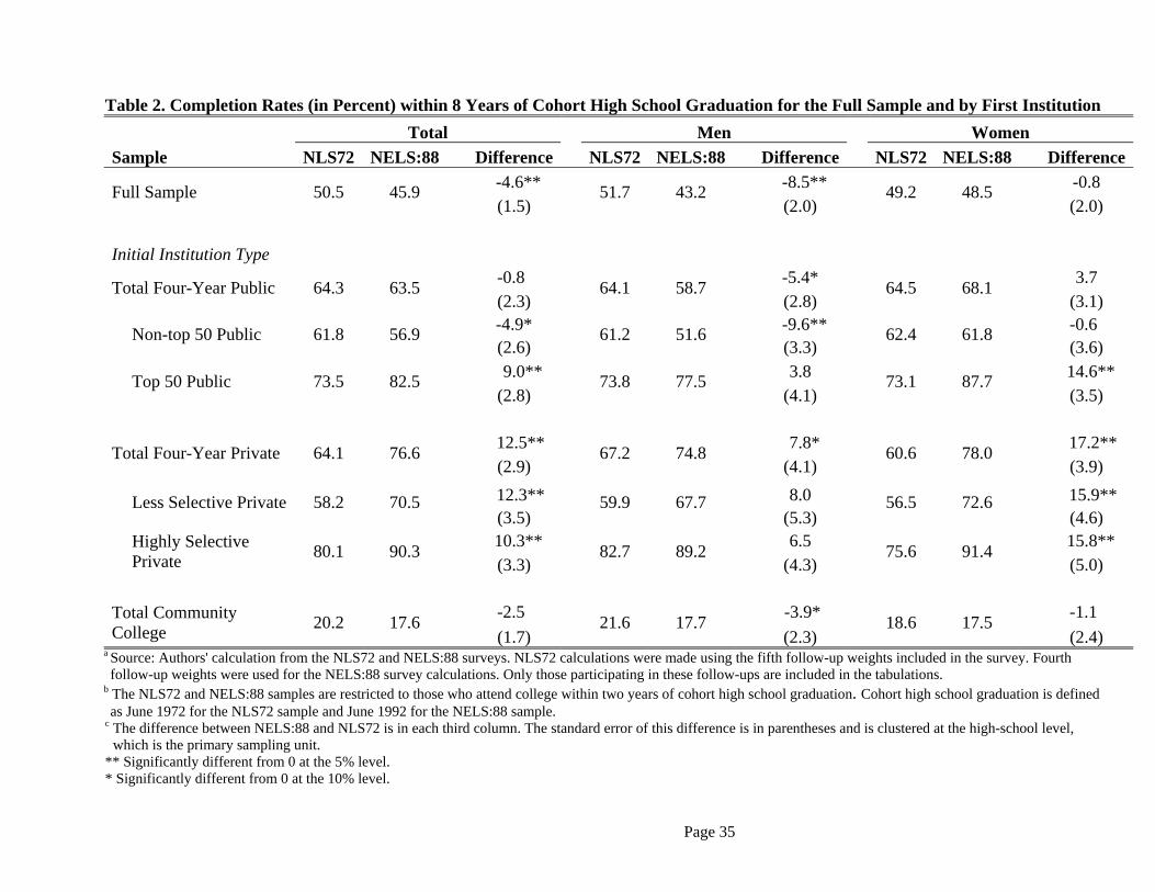
Page 35

Table 2. Completion Rates (in Percent) within 8 Years of Cohort High School Graduation for the Full Sample and by First Institution Total Men Women Sample NLS72 NELS:88 Difference NLS72 NELS:88 Difference NLS72 NELS:88 Difference

Full Sample 50.5 45.9

-4.6**

51.7 43.2

-8.5**

49.2 48.5

-0.8 (1.5) (2.0) (2.0)

Initial Institution Type

Total Four-Year Public 64.3 63.5 -0.8 64.1 58.7 -5.4* 64.5 68.1 3.7 (2.3) (2.8) (3.1)

Non-top 50 Public 61.8 56.9 -4.9* 61.2 51.6 -9.6** 62.4 61.8 -0.6

(2.6) (3.3) (3.6)

Top 50 Public 73.5 82.5 9.0** 73.8 77.5 3.8 73.1 87.7 14.6**

(2.8) (4.1) (3.5)

Total Four-Year Private 64.1 76.6 12.5** 67.2 74.8 7.8* 60.6 78.0 17.2** (2.9) (4.1) (3.9)

Less Selective Private 58.2 70.5 12.3** 59.9 67.7 8.0 56.5 72.6 15.9**

(3.5) (5.3) (4.6)

Highly Selective Private 80.1 90.3 10.3** 82.7 89.2 6.5 75.6 91.4 15.8**

(3.3) (4.3) (5.0)

Total Community College 20.2 17.6 -2.5 21.6 17.7 -3.9* 18.6 17.5 -1.1

(1.7) (2.3) (2.4) a Source: Authors' calculation from the NLS72 and NELS:88 surveys. NLS72 calculations were made using the fifth follow-up weights included in the survey. Fourth follow-up weights were used for the NELS:88 survey calculations. Only those participating in these follow-ups are included in the tabulations.

b The NLS72 and NELS:88 samples are restricted to those who attend college within two years of cohort high school graduation. Cohort high school graduation is defined as June 1972 for the NLS72 sample and June 1992 for the NELS:88 sample.

c The difference between NELS:88 and NLS72 is in each third column. The standard error of this difference is in parentheses and is clustered at the high-school level, which is the primary sampling unit.

** Significantly different from 0 at the 5% level. * Significantly different from 0 at the 10% level.

Page 36

Table 3. Means of Selected NLS72 and NELS:88 Variables

All College Attendees

College Graduates Who Obtain a BA With Eight Years of Cohort

High School Graduation Variable NLS72 NELS:88 NLS72 NELS:88 Bottom Math Test Quartile 0.112 0.156

0.057 0.039

Second Math Test Quartile 0.211 0.235 0.149 0.152 Third Math Test Quartile 0.270 0.282 0.256 0.289 Top Math Test Quartile 0.407 0.328 0.538 0.520 Math Test Percentile 62.545 58.014 70.677 71.711 Student-Faculty Ratio 29.524 39.069 25.504 29.807 Ln(Student-Faculty Ratio) 3.293 3.511 3.171 3.276 Missing S/F Ratio 0.108 0.108 0.099 0.052 Father’s Education

No HS Diploma 0.222 0.119 0.171 0.060 HS Diploma 0.261 0.304 0.222 0.207 Some College 0.243 0.225 0.247 0.222 BA 0.161 0.185 0.199 0.241 Graduate School 0.114 0.168 0.162 0.270

Mother’s Education No HS Diploma 0.180 0.114 0.133 0.055 HS Diploma 0.391 0.342 0.366 0.261 Some College 0.269 0.248 0.283 0.264 BA 0.117 0.176 0.154 0.247 Graduate School 0.043 0.119 0.064 0.173

Parental Income <3000/<10000 0.039 0.067 0.025 0.031 6000/20000 0.071 0.106 0.051 0.060 7500/25000 0.069 0.077 0.065 0.062 10500/35000 0.197 0.131 0.185 0.101 15000/50000 0.272 0.215 0.271 0.201 15000+/50000+ 0.351 0.404 0.403 0.545

Race/Ethnicity Asian 0.012 0.048 0.017 0.058 Hispanic 0.035 0.100 0.019 0.055 African American 0.092 0.110 0.073 0.074 White 0.861 0.742 0.891 0.813

Male 0.509 0.482 0.522 0.453 Number of Observations 7219 8280 4296 4140

a Source: Authors’ tabulations from the NELS:88 and NLS72 surveys. NLS72 calculations were made using the fifth follow-up weights included in the survey. Fourth follow-up weights were used for the NELS:88 survey calculations. Only those participating in these follow-ups are included in the tabulations.

b The NLS72 and NELS:88 samples are restricted to those who attend college within two years of cohort high school graduation. Cohort high school graduation is June 1972 in NLS72 and June 1992 in NELS:88.

c Parental income in NLS72 and NELS:88 are given in discrete ranges in both surveys. We group the income ranges into six income categories in each survey that correspond to the same real income across surveys using the CPI. In NLS72, the real income ranges are less than $3000, $3000-$6000, $6001-$7500, $7501-$10500, $10501-$15000, and greater than $15000. In NELS:88, the real income ranges are less than $10000, $10000-$20000, $20001-$25000, $25001-$35000, $35001-$50000, and greater than $50000.

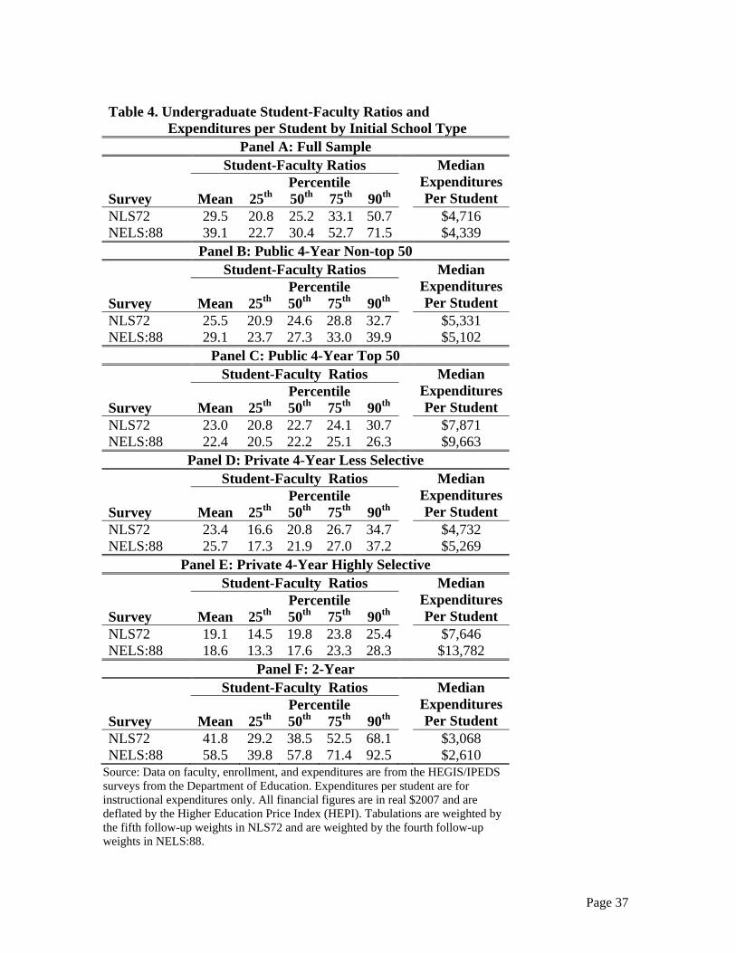
Page 37

Table 4. Undergraduate Student-Faculty Ratios and Expenditures per Student by Initial School Type

Panel A: Full Sample Student-Faculty Ratios Median

Expenditures Per Student

Percentile Survey Mean 25th 50th 75th 90th NLS72 29.5 20.8 25.2 33.1 50.7 $4,716 NELS:88 39.1 22.7 30.4 52.7 71.5 $4,339

Panel B: Public 4-Year Non-top 50 Student-Faculty Ratios Median

Expenditures Per Student

Percentile Survey Mean 25th 50th 75th 90th NLS72 25.5 20.9 24.6 28.8 32.7 $5,331 NELS:88 29.1 23.7 27.3 33.0 39.9 $5,102

Panel C: Public 4-Year Top 50 Student-Faculty Ratios Median

Expenditures Per Student

Percentile Survey Mean 25th 50th 75th 90th NLS72 23.0 20.8 22.7 24.1 30.7 $7,871 NELS:88 22.4 20.5 22.2 25.1 26.3 $9,663

Panel D: Private 4-Year Less Selective Student-Faculty Ratios Median

Expenditures Per Student

Percentile Survey Mean 25th 50th 75th 90th NLS72 23.4 16.6 20.8 26.7 34.7 $4,732 NELS:88 25.7 17.3 21.9 27.0 37.2 $5,269

Panel E: Private 4-Year Highly Selective Student-Faculty Ratios Median

Expenditures Per Student

Percentile Survey Mean 25th 50th 75th 90th NLS72 19.1 14.5 19.8 23.8 25.4 $7,646 NELS:88 18.6 13.3 17.6 23.3 28.3 $13,782

Panel F: 2-Year Student-Faculty Ratios Median

Expenditures Per Student

Percentile Survey Mean 25th 50th 75th 90th NLS72 41.8 29.2 38.5 52.5 68.1 $3,068 NELS:88 58.5 39.8 57.8 71.4 92.5 $2,610

Source: Data on faculty, enrollment, and expenditures are from the HEGIS/IPEDS surveys from the Department of Education. Expenditures per student are for instructional expenditures only. All financial figures are in real $2007 and are deflated by the Higher Education Price Index (HEPI). Tabulations are weighted by the fifth follow-up weights in NLS72 and are weighted by the fourth follow-up weights in NELS:88.

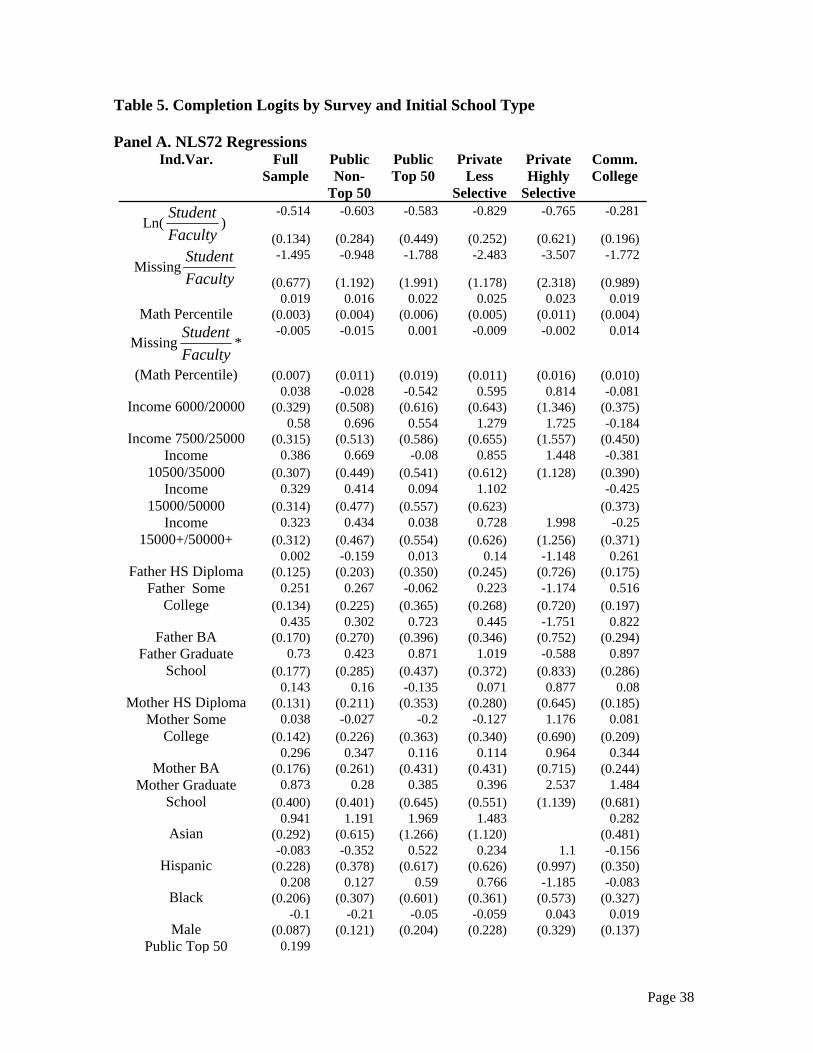
Page 38

Table 5. Completion Logits by Survey and Initial School Type Panel A. NLS72 Regressions

Ind.Var. Full Sample

Public Non-

Top 50

Public Top 50

Private Less

Selective

Private Highly

Selective

Comm. College

Ln(FacultyStudent

) -0.514 -0.603 -0.583 -0.829 -0.765 -0.281

(0.134) (0.284) (0.449) (0.252) (0.621) (0.196)

MissingFacultyStudent

-1.495 -0.948 -1.788 -2.483 -3.507 -1.772

(0.677) (1.192) (1.991) (1.178) (2.318) (0.989)

Math Percentile 0.019 0.016 0.022 0.025 0.023 0.019

(0.003) (0.004) (0.006) (0.005) (0.011) (0.004)

MissingFacultyStudent

*

(Math Percentile)

-0.005 -0.015 0.001 -0.009 -0.002 0.014

(0.007) (0.011) (0.019) (0.011) (0.016) (0.010)

Income 6000/20000 0.038 -0.028 -0.542 0.595 0.814 -0.081

(0.329) (0.508) (0.616) (0.643) (1.346) (0.375)

Income 7500/25000 0.58 0.696 0.554 1.279 1.725 -0.184

(0.315) (0.513) (0.586) (0.655) (1.557) (0.450) Income

10500/35000 0.386 0.669 -0.08 0.855 1.448 -0.381

(0.307) (0.449) (0.541) (0.612) (1.128) (0.390) Income

15000/50000 0.329 0.414 0.094 1.102 -0.425

(0.314) (0.477) (0.557) (0.623) (0.373) Income

15000+/50000+ 0.323 0.434 0.038 0.728 1.998 -0.25

(0.312) (0.467) (0.554) (0.626) (1.256) (0.371)

Father HS Diploma 0.002 -0.159 0.013 0.14 -1.148 0.261

(0.125) (0.203) (0.350) (0.245) (0.726) (0.175) Father Some

College 0.251 0.267 -0.062 0.223 -1.174 0.516

(0.134) (0.225) (0.365) (0.268) (0.720) (0.197)

Father BA 0.435 0.302 0.723 0.445 -1.751 0.822

(0.170) (0.270) (0.396) (0.346) (0.752) (0.294) Father Graduate

School 0.73 0.423 0.871 1.019 -0.588 0.897

(0.177) (0.285) (0.437) (0.372) (0.833) (0.286)

Mother HS Diploma 0.143 0.16 -0.135 0.071 0.877 0.08

(0.131) (0.211) (0.353) (0.280) (0.645) (0.185) Mother Some

College 0.038 -0.027 -0.2 -0.127 1.176 0.081

(0.142) (0.226) (0.363) (0.340) (0.690) (0.209)

Mother BA 0.296 0.347 0.116 0.114 0.964 0.344

(0.176) (0.261) (0.431) (0.431) (0.715) (0.244) Mother Graduate

School 0.873 0.28 0.385 0.396 2.537 1.484

(0.400) (0.401) (0.645) (0.551) (1.139) (0.681)

Asian 0.941 1.191 1.969 1.483 0.282

(0.292) (0.615) (1.266) (1.120) (0.481)

Hispanic -0.083 -0.352 0.522 0.234 1.1 -0.156

(0.228) (0.378) (0.617) (0.626) (0.997) (0.350)

Black 0.208 0.127 0.59 0.766 -1.185 -0.083

(0.206) (0.307) (0.601) (0.361) (0.573) (0.327)

Male -0.1 -0.21 -0.05 -0.059 0.043 0.019

(0.087) (0.121) (0.204) (0.228) (0.329) (0.137) Public Top 50 0.199

Page 39

(0.116) Private Less

Selective -0.252

(0.128) Private Highly

Selective 0.39

(0.167)

Community College -1.54

(0.104)

Constant 0.341 0.845 0.945 0.173 0.63 -1.696

(0.543) (0.996) (1.617) (0.991) (2.335) (0.908)

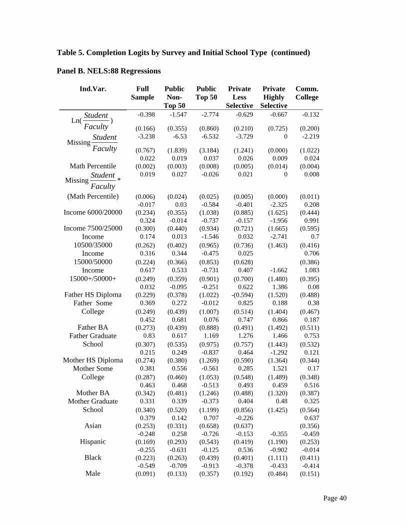
Page 40

Table 5. Completion Logits by Survey and Initial School Type (continued) Panel B. NELS:88 Regressions

Ind.Var. Full Sample

Public Non-

Top 50

Public Top 50

Private Less

Selective

Private Highly

Selective

Comm. College

Ln(FacultyStudent

) -0.398 -1.547 -2.774 -0.629 -0.667 -0.132

(0.166) (0.355) (0.860) (0.210) (0.725) (0.200)

MissingFacultyStudent

-3.238 -6.53 -6.532 -3.729 0 -2.219

(0.767) (1.839) (3.184) (1.241) (0.000) (1.022)

Math Percentile 0.022 0.019 0.037 0.026 0.009 0.024

(0.002) (0.003) (0.008) (0.005) (0.014) (0.004)

MissingFacultyStudent

*

(Math Percentile)

0.019 0.027 -0.026 0.021 0 0.008

(0.006) (0.024) (0.025) (0.005) (0.000) (0.011)

Income 6000/20000 -0.017 0.03 -0.584 -0.401 -2.325 0.208

(0.234) (0.355) (1.038) (0.885) (1.625) (0.444)

Income 7500/25000 0.324 -0.014 -0.737 -0.157 -1.956 0.991

(0.300) (0.440) (0.934) (0.721) (1.665) (0.595) Income

10500/35000 0.174 0.013 -1.546 0.032 -2.741 0.7

(0.262) (0.402) (0.965) (0.736) (1.463) (0.416) Income

15000/50000 0.316 0.344 -0.475 0.025 0.706

(0.224) (0.366) (0.853) (0.628) (0.386) Income

15000+/50000+ 0.617 0.533 -0.731 0.407 -1.662 1.083

(0.249) (0.359) (0.901) (0.700) (1.480) (0.395)

Father HS Diploma 0.032 -0.095 -0.251 0.622 1.386 0.08

(0.229) (0.378) (1.022) -(0.594) (1.520) (0.488) Father Some

College 0.369 0.272 -0.012 0.825 0.188 0.38

(0.249) (0.439) (1.007) (0.514) (1.404) (0.467)

Father BA 0.452 0.681 0.076 0.747 0.866 0.187

(0.273) (0.439) (0.888) (0.491) (1.492) (0.511) Father Graduate

School 0.83 0.617 1.169 1.276 1.466 0.753

(0.307) (0.535) (0.975) (0.757) (1.443) (0.532)

Mother HS Diploma 0.215 0.249 -0.837 0.464 -1.292 0.121

(0.274) (0.380) (1.269) (0.590) (1.364) (0.344) Mother Some

College 0.381 0.556 -0.561 0.285 1.521 0.17

(0.287) (0.460) (1.053) (0.548) (1.489) (0.348)

Mother BA 0.463 0.468 -0.513 0.493 0.459 0.516

(0.342) (0.481) (1.246) (0.488) (1.320) (0.387) Mother Graduate

School 0.331 0.339 -0.373 0.404 0.48 0.325

(0.340) (0.520) (1.199) (0.856) (1.425) (0.564)

Asian 0.379 0.142 0.707 -0.226 0.637

(0.253) (0.331) (0.658) (0.637) (0.356)

Hispanic -0.248 0.258 -0.726 -0.153 -0.355 -0.459

(0.169) (0.293) (0.543) (0.419) (1.190) (0.253)

Black -0.255 -0.631 -0.125 0.536 -0.902 -0.014

(0.223) (0.263) (0.439) (0.401) (1.111) (0.411)

Male -0.549 -0.709 -0.913 -0.378 -0.433 -0.414

(0.091) (0.133) (0.357) (0.192) (0.484) (0.151)

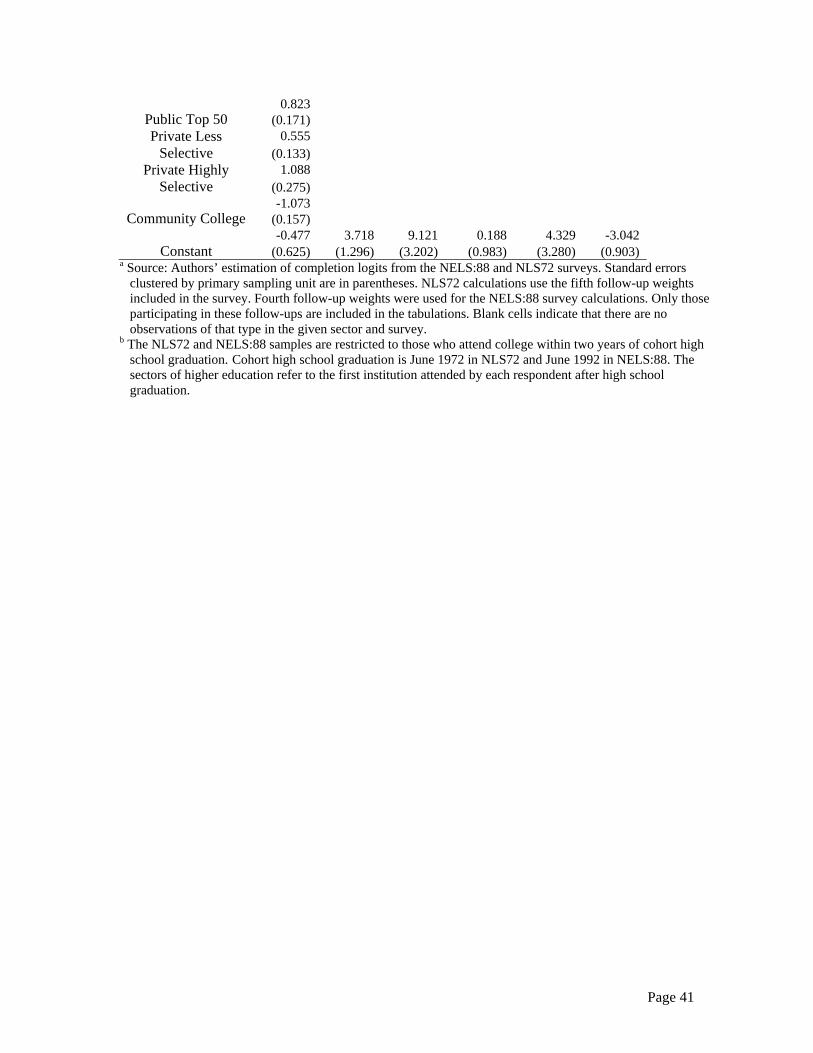
Page 41

Public Top 50 0.823

(0.171) Private Less

Selective 0.555

(0.133) Private Highly

Selective 1.088

(0.275)

Community College -1.073

(0.157)

Constant -0.477 3.718 9.121 0.188 4.329 -3.042

(0.625) (1.296) (3.202) (0.983) (3.280) (0.903) a Source: Authors’ estimation of completion logits from the NELS:88 and NLS72 surveys. Standard errors

clustered by primary sampling unit are in parentheses. NLS72 calculations use the fifth follow-up weights included in the survey. Fourth follow-up weights were used for the NELS:88 survey calculations. Only those participating in these follow-ups are included in the tabulations. Blank cells indicate that there are no observations of that type in the given sector and survey.

b The NLS72 and NELS:88 samples are restricted to those who attend college within two years of cohort high school graduation. Cohort high school graduation is June 1972 in NLS72 and June 1992 in NELS:88. The sectors of higher education refer to the first institution attended by each respondent after high school graduation.

Page 42

Table 6. Logit Simulation Decompositions based on NELS:88 Estimates of College Completion by Type of Institution

Full

Sample

Public Non-Top

50 Public Top 50

Private Less

Selective

Private Highly

Selective Community

College NLS72 50.5 61.8 73.5 58.2 80.1 20.2

NELS:88 45.9 56.9 82.5 70.5 90.3 17.6 Total Change -4.6 -4.9 9.0 12.3 10.3 -2.5

Change Due to Observables (X) -4.5 -0.6 3.7 3.2 11.0 -3.6 Change Due to Student Characteristics 0.1 3.4 2.6 3.8 10.4 -3.1 Math Test Percentiles -1.6 0.3 0.6 -0.1 0.2 -2.2 Other Student Characteristics 1.7 3.1 2.0 3.9 10.2 -0.9

Change Due to Supply-Side Factors -4.6 -4.0 1.1 -0.6 0.6 -0.5 Student-Faculty Ratios -1.1 -4.0 1.1 -0.6 0.6 -0.5 Initial School Types -3.5

Residual -0.1 -4.3 5.3 9.1 -0.8 1.0 a Source: Authors’ calculations as described in the text from the NLS72 and NELS:88 surveys . NLS72 calculations were made using the fifth follow-up weights included

in the survey. Fourth follow-up weights were used for the NELS:88 survey calculations. Only those participating in these follow-ups are included in the regression. School type samples refer to first institution attended. The NLS72 and NELS:88 samples are restricted to those who attend college within two years of cohort high school graduation. Cohort high school graduation is defined as June 1972 for the NLS72 sample and June 1992 for the NELS:88 sample.

b The Change Due to Observables is the difference between the observed NELS:88 completion rate and the simulated NELS:88 completion rate using the distribution of all observables from NLS72. The changes due to math test percentiles, student-faculty ratios and initial school types are the differences between the observed NELS:88 completion rate and the simulated NELS:88 completion rates in which we simulate the completion rate if the each variable were distributed as in the NLS72 survey and all other observables were unchanged. The Change Due to Supply Side Factors is the sum of the changes due to student-faculty ratios and initial school types. We calculate the Change Due to Student Characteristics as the difference between the Change Due to Observables (X) and the Change Due to Supply-Side Factors. The Change Due to Other Student Characteristics is calculated by subtracting the Change Due to Math Test Percentiles from the Change Due to Student Characteristics.

c Data on faculty and enrollment are from the HEGIS/IPEDS surveys from the Department of Education.

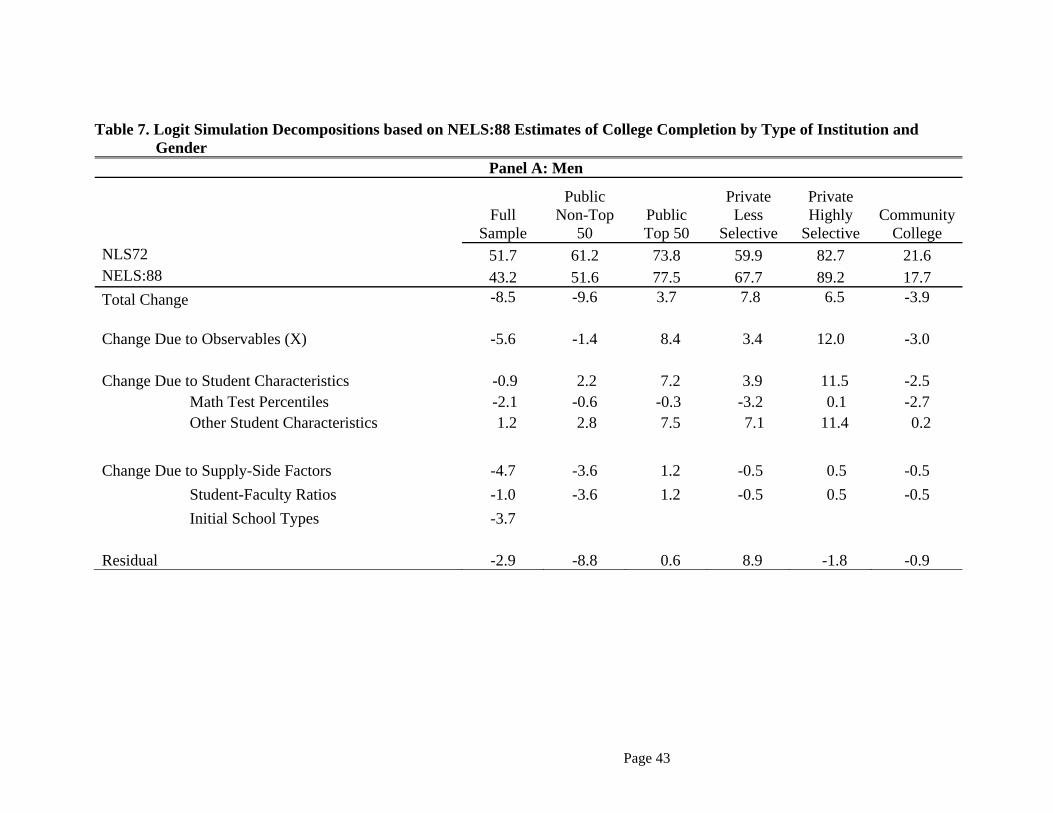
Page 43

Table 7. Logit Simulation Decompositions based on NELS:88 Estimates of College Completion by Type of Institution and Gender

Panel A: Men

Full Sample

Public Non-Top

50 Public Top 50

Private Less

Selective

Private Highly

Selective Community

College NLS72 51.7 61.2 73.8 59.9 82.7 21.6 NELS:88 43.2 51.6 77.5 67.7 89.2 17.7 Total Change -8.5 -9.6 3.7 7.8 6.5 -3.9

Change Due to Observables (X) -5.6 -1.4 8.4 3.4 12.0 -3.0 Change Due to Student Characteristics -0.9 2.2 7.2 3.9 11.5 -2.5 Math Test Percentiles -2.1 -0.6 -0.3 -3.2 0.1 -2.7 Other Student Characteristics 1.2 2.8 7.5 7.1 11.4 0.2 Change Due to Supply-Side Factors -4.7 -3.6 1.2 -0.5 0.5 -0.5 Student-Faculty Ratios -1.0 -3.6 1.2 -0.5 0.5 -0.5 Initial School Types -3.7

Residual -2.9 -8.8 0.6 8.9 -1.8 -0.9

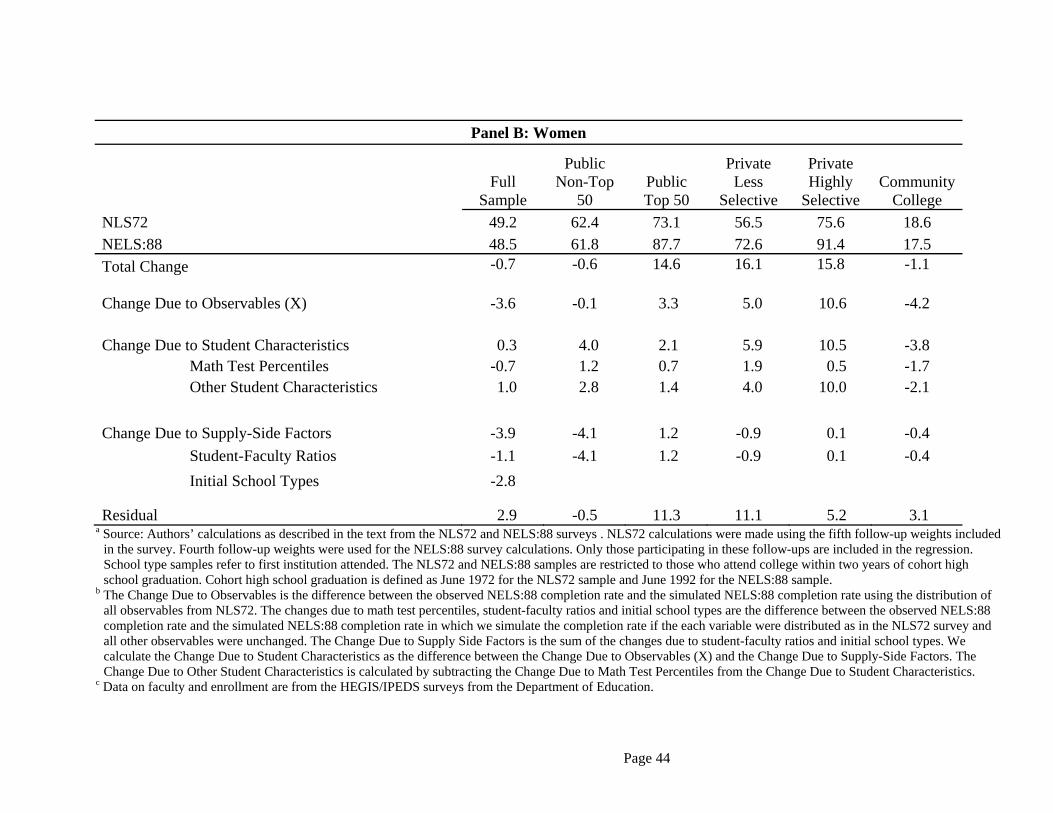
Page 44

Panel B: Women

Full Sample

Public Non-Top

50 Public Top 50

Private Less

Selective

Private Highly

Selective Community

College NLS72 49.2 62.4 73.1 56.5 75.6 18.6 NELS:88 48.5 61.8 87.7 72.6 91.4 17.5 Total Change -0.7 -0.6 14.6 16.1 15.8 -1.1

Change Due to Observables (X) -3.6 -0.1 3.3 5.0 10.6 -4.2 Change Due to Student Characteristics 0.3 4.0 2.1 5.9 10.5 -3.8 Math Test Percentiles -0.7 1.2 0.7 1.9 0.5 -1.7 Other Student Characteristics 1.0 2.8 1.4 4.0 10.0 -2.1 Change Due to Supply-Side Factors -3.9 -4.1 1.2 -0.9 0.1 -0.4 Student-Faculty Ratios -1.1 -4.1 1.2 -0.9 0.1 -0.4 Initial School Types -2.8

Residual 2.9 -0.5 11.3 11.1 5.2 3.1 a Source: Authors’ calculations as described in the text from the NLS72 and NELS:88 surveys . NLS72 calculations were made using the fifth follow-up weights included

in the survey. Fourth follow-up weights were used for the NELS:88 survey calculations. Only those participating in these follow-ups are included in the regression. School type samples refer to first institution attended. The NLS72 and NELS:88 samples are restricted to those who attend college within two years of cohort high school graduation. Cohort high school graduation is defined as June 1972 for the NLS72 sample and June 1992 for the NELS:88 sample.

b The Change Due to Observables is the difference between the observed NELS:88 completion rate and the simulated NELS:88 completion rate using the distribution of all observables from NLS72. The changes due to math test percentiles, student-faculty ratios and initial school types are the difference between the observed NELS:88 completion rate and the simulated NELS:88 completion rate in which we simulate the completion rate if the each variable were distributed as in the NLS72 survey and all other observables were unchanged. The Change Due to Supply Side Factors is the sum of the changes due to student-faculty ratios and initial school types. We calculate the Change Due to Student Characteristics as the difference between the Change Due to Observables (X) and the Change Due to Supply-Side Factors. The Change Due to Other Student Characteristics is calculated by subtracting the Change Due to Math Test Percentiles from the Change Due to Student Characteristics.

c Data on faculty and enrollment are from the HEGIS/IPEDS surveys from the Department of Education.

Page 45

Table 8. State-level Estimates of the Effect of Crowding on Completion Rates, 1940-1975 Birth Cohorts Observed in the 2000 U.S. Census

Independent Variable: Log of State Birth Cohort Population Dependent Variable: ln (BA/Some College) Un-weighted Weighted

All -0.112** -0.165** -0.125** -0.185**(0.019) (0.045) (0.023) (0.034)

Males -0.120** -0.230** -0.137** -0.191**(0.026) (0.072) (0.022) (0.057)

Females -0.101** -0.104 -0.109** -0.177**(0.021) (0.063) (0.030) (0.037)

State-Specific Trends? No Yes No Yes

a Source: 1940-1975 birth cohorts of non-immigrants from the 2000 U.S. Census. Each table entry reflects a separate regression. Each regression includes 1728 state x year cells.

b All regressions are at the state level and include state and birth cohort fixed effects. Alaska, Hawaii, and Washington, DC are excluded from the analysis.

c Weighted regressions are weighted with the average cohort size in each state across the 1940-1975 birth cohorts.

d Standard errors are in parentheses and are clustered at the state level. ** Significantly different from 0 at the 5% level.

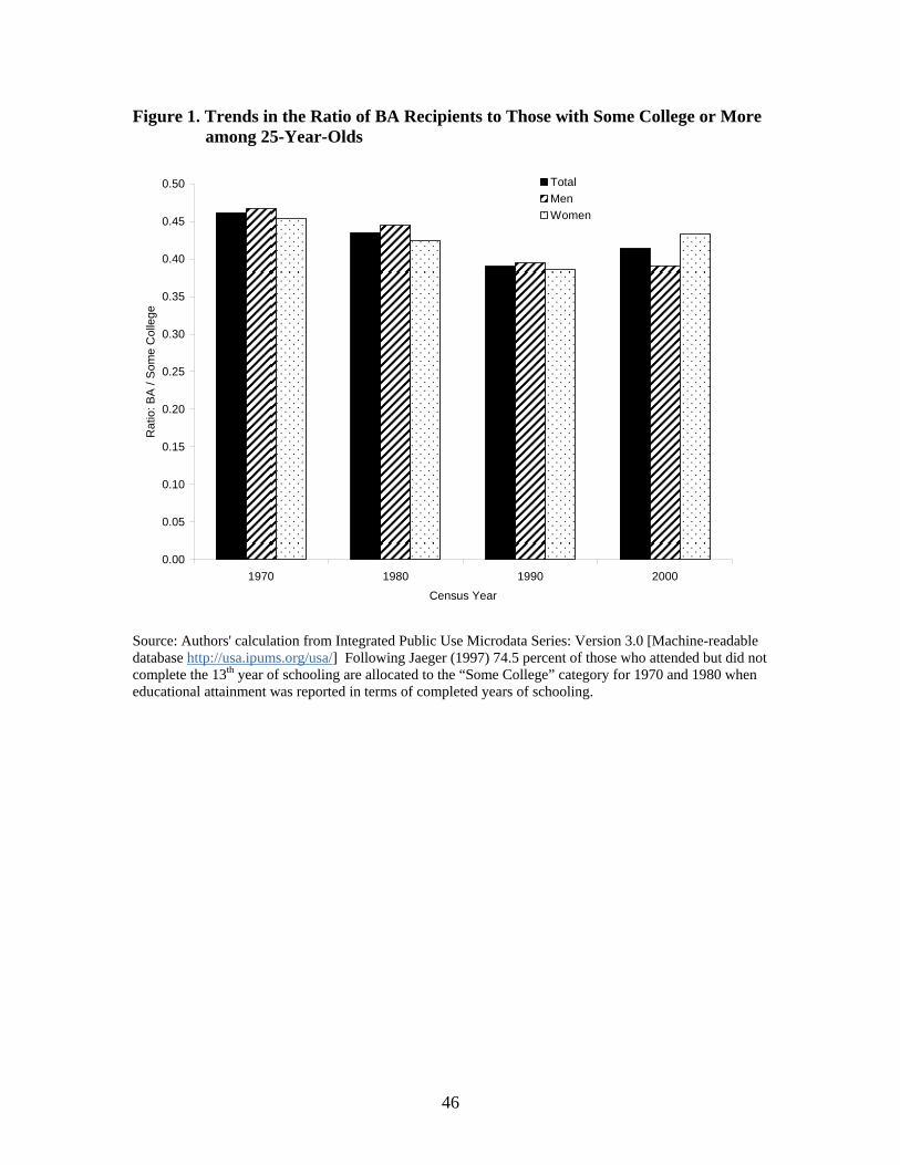
46

Figure 1. Trends in the Ratio of BA Recipients to Those with Some College or More among 25-Year-Olds

0.00

0.05

0.10

0.15

0.20

0.25

0.30

0.35

0.40

0.45

0.50

1970 1980 1990 2000

Census Year

Rat

io: B

A /

Som

e C

olle

ge

TotalMenWomen

Source: Authors' calculation from Integrated Public Use Microdata Series: Version 3.0 [Machine-readable database http://usa.ipums.org/usa/] Following Jaeger (1997) 74.5 percent of those who attended but did not complete the 13th year of schooling are allocated to the “Some College” category for 1970 and 1980 when educational attainment was reported in terms of completed years of schooling.

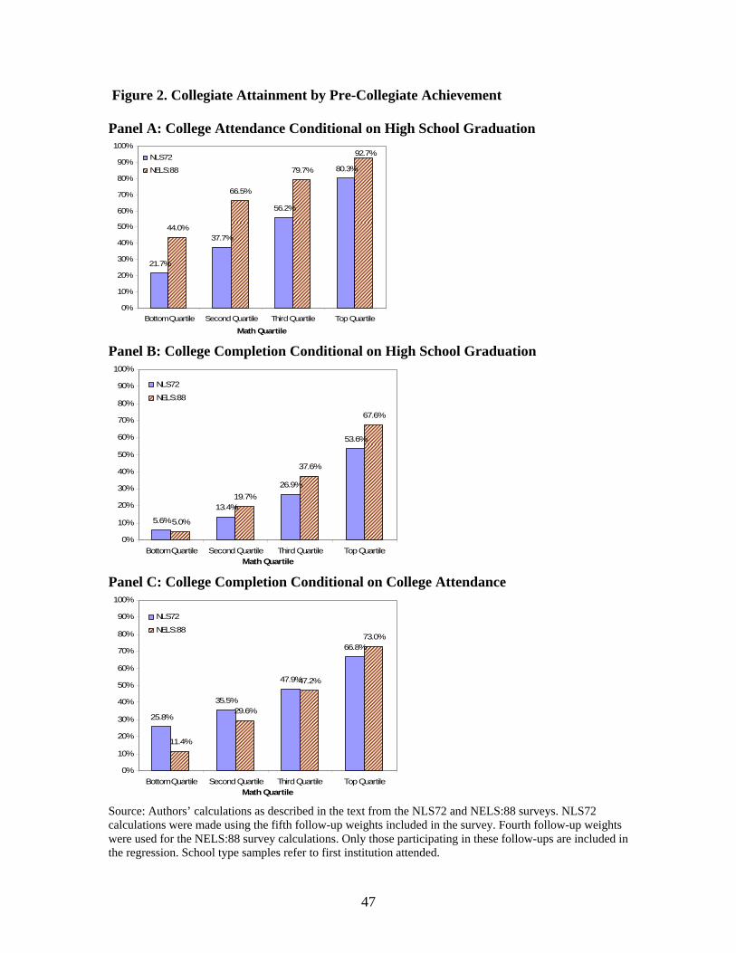
47

Figure 2. Collegiate Attainment by Pre-Collegiate Achievement Panel A: College Attendance Conditional on High School Graduation

21.7%

37.7%

56.2%

80.3%

44.0%

66.5%

79.7%

92.7%

0%

10%

20%

30%

40%

50%

60%

70%

80%

90%

100%

Bottom Quartile Second Quartile Third Quartile Top Quartile

Math Quartile

NLS72

NELS:88

Panel B: College Completion Conditional on High School Graduation

5.6%

13.4%

26.9%

53.6%

5.0%

19.7%

37.6%

67.6%

0%

10%

20%

30%

40%

50%

60%

70%

80%

90%

100%

Bottom Quartile Second Quartile Third Quartile Top QuartileMath Quartile

NLS72

NELS:88

Panel C: College Completion Conditional on College Attendance

25.8%

35.5%

47.9%

66.8%

11.4%

29.6%

47.2%

73.0%

0%

10%

20%

30%

40%

50%

60%

70%

80%

90%

100%

Bottom Quartile Second Quartile Third Quartile Top QuartileMath Quartile

NLS72

NELS:88

Source: Authors’ calculations as described in the text from the NLS72 and NELS:88 surveys. NLS72 calculations were made using the fifth follow-up weights included in the survey. Fourth follow-up weights were used for the NELS:88 survey calculations. Only those participating in these follow-ups are included in the regression. School type samples refer to first institution attended.

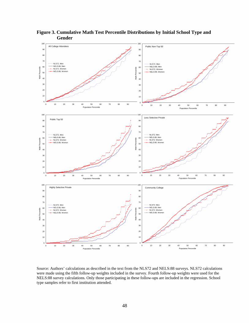
48

Figure 3. Cumulative Math Test Percentile Distributions by Initial School Type and Gender

0

10

20

30

40

50

60

70

80

90

100

0 10 20 30 40 50 60 70 80 90Population Percentile

Mat

h P

erce

ntile

NLS72, MenNELS:88, MenNLS72, WomenNELS:88, Women

All College Attendees

0

10

20

30

40

50

60

70

80

90

100

0 10 20 30 40 50 60 70 80 90

Population Percentile

Mat

h P

erce

ntile

NLS72, MenNELS:88, MenNLS72, WomenNELS:88, Women

Public Non-Top 50

0

10

20

30

40

50

60

70

80

90

100

0 10 20 30 40 50 60 70 80 90

Population Percentile

Mat

h P

erce

ntile

NLS72, MenNELS:88, MenNLS72, WomenNELS:88, Women

Public Top 50

0

10

20

30

40

50

60

70

80

90

100

0 10 20 30 40 50 60 70 80 90Population Percentile

Mat

h P

erce

ntile

NLS72, MenNELS:88, MenNLS72, WomenNELS:88, Women

Less Selective Private

0

10

20

30

40

50

60

70

80

90

100

0 10 20 30 40 50 60 70 80 90

Population Percentile

Mat

h P

erce

ntile

NLS72, MenNELS:88, MenNLS72, WomenNELS:88, Women

Highly Selective Private

0

10

20

30

40

50

60

70

80

90

100

0 10 20 30 40 50 60 70 80 90Population Percentile

Mat

h P

erce

ntile

NLS72, MenNELS:88, MenNLS72, WomenNELS:88, Women

Community College

Source: Authors’ calculations as described in the text from the NLS72 and NELS:88 surveys. NLS72 calculations were made using the fifth follow-up weights included in the survey. Fourth follow-up weights were used for the NELS:88 survey calculations. Only those participating in these follow-ups are included in the regression. School type samples refer to first institution attended.

49

Supplemental Online Appendices Appendix A: Technical Appendix

I. NLS72 and NELS:88 Data

a. Degree Completion Degree completion is calculated using National Longitudinal Study of the High School

Class of 1972 (NLS72) and the National Educational Longitudinal Study of 1988 (NELS:88) survey responses from the first through fifth follow-ups in NLS72 and the fourth follow-up in NELS:88. The NLS72 study participants were seniors in high school in the spring of 1972. Following the base year interview, participant follow-up surveys were administered in 1973, 1974, 1976, 1979, and 1986 (for a subsample), with questions covering collegiate participation and degree attainment. In addition, detailed high school records and postsecondary transcripts were collected by the Department of Education.

The NELS:88 survey started with students who were in the eighth grade in 1988 (high school class of 1992) and conducted follow-up surveys with participants in 1990, 1992, 1994, and 2000. Similar to the NLS72 survey, NELS:88 contains high school records and collegiate transcripts as well as a host of background information that may be relevant to degree completion.

Degree completion is defined as obtaining a BA within 8 years of cohort high school graduation conditional on beginning college within 2 years of cohort high school graduation. Cohort high school graduation is defined as June 1972 for the NLS72 sample and June 1992 for the NELS:88 sample.

Because the NELS:88 survey is comprised of eighth graders from 1988 and the NLS72 survey follows 12th graders from the class of 1972, the NELS:88 survey contains more students who graduate high school after their cohort’s high school graduation. In our base sample, 1.3% of respondents in NLS72 and 4.4% of respondents in NELS:88 finish high school after June of their respective cohort graduation year. However, looking only at eight-year BA recipients, 0.3% and 0.6%, respectively in NLS72 and NELS:88 did not finish high school on time, and few of these students entered college within 2 years of cohort high school graduation. It is therefore unlikely the larger preponderance of late high school graduates in the NELS:88 survey biases our completion rate calculations.

Table A-1 of this Appendix contains variable names and definitions used to define the sample and to calculate degree completion in both the NLS72 and NELS:88 surveys.

b. School Type and Collegiate Start Dates We define enrollment as those who start at an academic institution within two years of

cohort high school graduation. Academic institutions are all four-year schools and public two-year schools. We exclude private two-year schools because they typically are not oriented towards allowing students to obtain a BA post-graduation.

College transcript data and self-reported enrollment records from the first through fourth follow-up surveys for the NLS72 survey and from NCES-aggregated responses in the NELS:88 survey are used to define the type of institution of initial collegiate enrollment. We use the transcript for the first institution post-high school attended by respondents in the transcript files

50

to assign first institution attended for most respondents. In the cases in which there are multiple first transcripts from different institutions on the same date, we assign each student to the school at which she took the most credits during the first semester. There are some students who report attending college within two years of their cohort’s high school graduation but do not have any transcripts. In NLS72, 6.8% of the sample reporting attendance do not have transcripts, and in NELS:88, 8.2% of the sample falls into this category. For these respondents, we use the first institution reported by them in the survey files.

In the NLS72 survey, we begin by determining the year in which a student first enrolls in an academic post-secondary institution, where “academic” is defined as granting at least an associates degree or BA. In each follow-up, students were asked about colleges they attended (up to three) in each year since the previous survey. The first college attended is identified from the entry the first time a student reports attending an academic institution and we record the institutional identifier (FICE code) either directly from transcript files or from the student survey responses about which institution they attended. We then merge institutional-level information that contains public/private status, 2-year/4-year identifiers, and collegiate rankings and classify the respondent’s initial institution accordingly.

In the NELS:88 survey, we use a similar methodology to identify each respondent’s initial institution. NCES has constructed variables that identify first institution attended in the transcript files (the “ref” variables). We use the transcript-based NCES-constructed institutional identifier (“unitid”) code when it is available. For those who report college attendance and the sector of first attendance but are not assigned a transcript-based first institution identifier by NCES, we use the NCES-constructed variables that report individual enrollment histories from the survey data that identify first institution of enrollment (“unitid”) and first institution type (“f4efsect”).

For students with post-secondary experience preceding high school graduation, we use the first start date and institution after high school graduation taken from the post-secondary transcript files. For all other students in the NELS:88 survey, first start date is identified by f4efmy, which is the NCES-constructed date of first post-secondary attendance.

A list of the top-50 public schools from the 2005 U.S. News and World Report rankings as well as the top-65 private schools and the top-50 liberal arts colleges plus the United States Armed Services Academies, which constitute the highly selective private schools, is shown is shown in Table A-2.

c. Background Characteristics

i. Math Tests

In both surveys, tests of academic achievement were administered to students in the senior year. The NLS72 exam was administered as a 69-minute test book with sections on vocabulary, picture numbers (associative memory), reading, letter groups, mathematics, and mosaic comparisons. Each section was 15 minutes (except for the mosaic comparison, which was 9 minutes). The math test included 25 items and contained only quantitative comparisons in order to measure basic quantitative competence. We use the reported scaled math score (scmatsc) test score measure in NLS72.

The NELS:88 cognitive test batteries were administered in each of the first three waves, with sections on reading, math, science and social studies. The tests were 85 minutes and consisted of 116 questions, 40 of which were on math and 21 of which were on reading

51

comprehension. Unlike the NLS72 exams, the NELS:88 tests covered more material and tested more skills. The math exam consisted of word problems, graphs, equations, quantitative comparisons, and geometric figures. Further, because the NELS:88 tests were given in subsequent waves, students were given harder or easier tests in the first and second follow-ups depending on their scores in the previous wave to guard against floor and ceiling effects. We use the math IRT theta score (f22xmth) from the second follow-up as the base measure of test scores. These scores are psychometric evaluation scores of each student’s ability that account for the difficulty of the exam.

Because the tests in NLS72 and NELS:88 covered different subject matter, were of different lengths, and were graded on different scales, the scores are not directly comparable across surveys. Instead, we construct the percentile of the score distribution for each survey among all high school graduates. The comparison of students in the same test percentile across surveys is based on the assumption overall achievement did not change over this time period. This assumption is supported by the observation that there is little change in the overall level of test scores on the nationally-representative NAEP over our period of observation. Similarly, examination of time trends in standard college entrance exams such as the SAT provides little support for the proposition that achievement declined appreciable over the interval. For the SAT, the ratio of test takers to high school graduates increased from 33% to 42%, while mean math scores declined from 509 to 501 over the 1972 to 1992 interval (Digest of Education Statistics, 2005, Table 129).

In the NLS72 survey, we use high school GPA as an imputation variable in order to measure pre-collegiate academic ability for students with missing test scores. The GPA measure we use is “imptaver” from the NLS72 survey. In the multiple imputation of missing variables in the NELS:88 survey, we use IRT theta test scores from the first follow-up for math (f12xmth) and from the base year for math (by2xmth). The IRT theta scores are scaled to a common metric across years by NCES. The imputed math test scores from the senior year in each survey are used to construct the test percentiles used in the main analysis.

ii. Parental Education

We obtain student reported measures of father’s and mother’s education separately. In the NLS72 survey, we have three different measures of this variable. For mother’s education, we use the variables cmoed, bq90b, and fq78b. For father’s education, we use the variables cfaed, bq90a, and fq78a. If there are disagreements across measures, fq78b and fq78a take precedence.

In the NELS:88 survey, we also use student reports of father’s education (bys34a) and mother’s education (bys34b). For the multiple imputation model, we include parent self-reports of their own education from the base year and second follow-up parental surveys. In the base year parent survey, we combine information on whether the respondent and his/her spouse is the father or mother (byp1a1 and byp1a2) with reported self (byp30) and spouse (byp31) educational attainment. A similar methodology is used for the second-follow up parent survey, using f2p1a and f2p1b to identify the gender of the respondent and the spouse, respectively, and f2p101a and f2p101b to identify educational attainment of the respondent and the spouse, respectively. The base year and second follow-up parental education information is aggregated into two variables, father’s education and mother’s education, used in the multiple imputation model.

iii. Parental Income Levels

52

The parental income variables are bq93 for NLS72 and f2p74 for NELS:88. The former is reported by the student while the latter is reported by the parents. Unfortunately, NLS72 does not contain a parent-reported measure and the NELS:88 survey does not contain a student-reported measure, so these variables are the most closely aligned parental income measures across the two surveys.

Rather than asking directly for parental income levels, the NELS:88 and NLS72 surveys ask for income ranges from respondents. Because we are interested in measuring parents’ ability to finance college, the variable of interest is the real income level, not one’s place in the income distribution. We thus align the income blocks across the two surveys using the CPI. In NLS72, the measured income groups we construct are less than $3000, $3000-$6000, $6000-$7500, $7500-$10500, $10500-$15000, and greater than $15000. In NELS:88, the corresponding real income blocks we create are less than $10000, $10000-$20000, $20000-$25000, $25000-$35000, $35000-$50000, and greater than $50000. Across surveys, the six income groups are comparable in real terms.

iv. Race Race is measured in the NLS72 survey using “crace” and “race86.” The latter is used if

the former is blank due to non-response. In the NELS:88 survey, race is measured using the “race” variable available in the data files.

II. Procedures to Handle Missing Data

d. Multiple Imputation

There is a considerable amount of missing data in the NLS72 and NELS:88 surveys. Table A-3 of this Appendix presents the number of unweighted missing observations by variable and survey. These observations are not missing completely at random; respondents who have no math test scores are less likely to finish college conditional on starting.

Casewise deletion of missing observations will therefore cause a bias in the calculation of the base trends we are seeking to explain in this analysis. To deal with this problem, we use the multiple imputation by chained equation (MICE) algorithm developed by Van Buuren, Boshuizen, and Knook (1999) that is implemented through the STATA module “ICE” (see Royston (2004) for a detailed discussion of ICE).

MICE is implemented by first defining the set of predictor variables (x1…xk) and the set of variables with missing values to be imputed: math test scores, father’s education, mother’s education, and parental income levels (y1…y5). The MICE algorithm implemented by ICE first randomly fills in all missing values from the posterior distribution of each variable. Then, for each variable with missing data, yi, STATA runs a regression (or ordered logit) of yi on y~i and x1…xk and calculates expected values from these regressions for all missing data points. The expected values then replace the randomly assigned values for the missing data points. A sequence of regressions for each yi is a cycle, and this process is repeated for 10 cycles, replacing the missing values with the new expected values from each regression in each cycle. The imputed values after 10 cycles constitute one imputed data set, and this process is repeated five different times to generate five imputed data sets.

There are two important specifications in implementing MICE: determination of the predictor variables and determination of the imputation models. Because of the different

53

structure of the two surveys, different variables are used in the imputation procedure across surveys. In both surveys, we include dummy variables for cumulative time to degree from four to eight years, dummy variables for initial school type, interactions between these variables, an indicator for college attendance within two years of cohort high school graduation, as well as race and gender indicators.

For imputations with the NLS72 sample, we include a measure of high school GPA in order to proxy for unobserved ability among those without test score information. Due to the structure of the NELS:88 survey, there is more background information with which to impute missing data. We use 8th and 10th grade math test scores, parental reports of their education from the base year and second follow-up parent surveys, and parental reports of their income level from the base year parent survey. The definitions of the variables used in the imputation models are discussed in the preceding section.

Because the math test scores are continuous variables, we use OLS regressions to impute these variables. Mother’s and father’s education and income, however, are categorical variables. Because of the ordered nature of these variables, we use ordered logits to impute the missing values of these variables. While these model choices are reasonably arbitrary, they are only used to draw ranges of plausible estimates of missing data.

The multiple imputation procedure creates five different data sets, each with different imputed values for the missing observations. All reported statistics and results in our analysis are averages across data sets. In other words, we conduct each analysis separately for each data set and average the final result. The average of final results is what is reported in the tables and figures in the paper. For the completion logit estimates in Table 5, we use the “micombine” command in STATA that is designed to estimate coefficients and standard errors from multiply imputed data sets. The coefficient estimates represent the simple arithmetic mean across the five coefficients from each imputed data set for each variable. Standard error estimation in this context is more complex. See Carlin et al. (2003) for a complete description of how standard errors are calculated.

e. Dropped Observations and Missing Transcript Data

The base sample in this analysis consists of all respondents who graduate high school and

attend college within two years of their cohort’s high school graduation. We further restrict the sample to exclude those whose only enrollment over this time period is at a private two-year institution as these schools are predominantly professional without a BA track. Table A-4 presents information on the number of observations that are dropped by survey and the reason for dropping the observation. For example, 168 respondents are dropped because they are not high school graduates in NLS72 whereas 720 are dropped in NELS:88 for this reason. The apparently higher dropout rate in NELS:88 is because the universe of students are all those enrolled in the 8th grade in 1988, whereas the universe in NLS72 are all those enrolled in 12th grade in 1972.

In the NLS72 survey, 63 observations are dropped because they report attending college but provide no information on either the type of institution or the date they first began attending this institution, and in NELS:88, 50 respondents do not provide this information. In addition, 200 observations were dropped because they were not in all four waves of the NELS:88 survey. In other words, they have a sample weight of zero.

54

Of potential concern in constructing our sample is the exclusion of those beginning college more than two years post-high school cohort graduation. We exclude these observations because we are interested in the truncated, eight-year completion rate. These statistics have a different interpretation for a student who began college directly after high school than for a student who began college, for instance, five years after high school. In NLS72, 889 respondents attend college more than 2 years after their cohort’s high school graduation, and in NELS:88, 970 do so. Given the similarity of these numbers, shifts in when students began attending college cannot account for the trends in completion rates reported in the main text.

III. Counterfactual Simulation Procedure

The counterfactual math test scores, student-faculty ratios and initial school types are

computed using a matching algorithm that holds relative rank constant. The goal of this procedure is to generate a counterfactual of the variable X on the NELS:88 sample that has the same distribution as the variable in the NLS72 sample. To construct this counterfactual, we first expand both data sets based on the analysis sample weights and then balance the two surveys by randomly deleting observations from the survey with more weighted observations. The weight-expanded samples then have the same number of observations in each survey. We then use the psmatch2 program in STATA to match each NELS:88 respondent to a NLS72 respondent on the variable X, using single nearest neighbor matching without replacement. For each NELS:88 respondent, we assign a counterfactual value of X that is equal to the value from the unique match. This matching method creates a counterfactual distribution of X in the NELS:88 sample that has the same mean as in the NLS72 sample and has a distribution that holds relative rank-order constant across the surveys. Using single nearest neighbor matching on X without replacement with psmatch2 ensures that we are finding a unique match for each NELS:88 respondent and that we are breaking ties randomly. Finally, we collapse the data back down to the individual level to conduct our analyses.

Because the math test percentiles we use are multiply imputed, we perform this procedure separately for each imputed data set. However, the imputations are done separately by survey, so it is not correct to match similarly numbered imputations with each other across cohorts. Instead, for each imputation in NELS:88, we perform our matching algorithm separately for each imputation in NLS72 and take the average counterfactual math test percentile across NLS72 imputations for each NELS:88 imputation. This procedure requires us to perform the matching algorithm 25 times when we simulate counterfactual math test percentiles.

When we simulate counterfactual student-faculty ratios and initial school types, we only have to conduct the matching algorithm once because none of the data are imputed. But, for student-faculty ratios, there are a number of missing observations. To handle this difficulty, we treat missing status as a fixed attribute and perform the matching only for observations with non-missing student-faculty ratio values. For those with missing student-faculty ratios, they are assumed to have missing data both in the observed and counterfactual completion rate calculations.

With test score percentiles and student-teacher ratios, establishing rank-order is straightforward as these variables are cardinal. For initial school type, however, how to rank-order the samples is less clear. For the matching procedure, we order school types in ascending order from least to most selective. Thus, school type 1 is community colleges, followed by non-top 50 public universities, less selective private universities, top 50 public schools, and finally

55

highly selective private universities. The logic behind this ordering is that we are assigning students in our counterfactual simulations to sectors that are most similar to their observed sector; we are not assigning, for example, students in community colleges to the highly selective private sector when finding counterfactual school types. This ordering creates conservative estimates of the effect of school type shifts on completion rates because we are minimizing the quality increases for each student associated with the shift across sectors that has occurred over time.

References

Carlin, John B., Ning Li, Philip Greenwood, and Carolyn Coffey. 2003. “Tools for Analyzing Multiple Imputed Datasets.” Stata Journal, 3(3): 226-244. Royston, Patrick. 2004. “Multiple Imputation of Missing Values.” Stata Journal, 4(3): 227-241. Van Buuren, Stef, Hendriek C. Boshuizen, and Dick L. Knook. 1999. “Multiple Imputation of Missing Blood Pressure Covariates in Survival Analysis.” Statistics in Medicine, 18(6): 681-694.

56

Table A-1. Variable Names and Definitions for Calculation of Completion Rates in NLS72 and NELS:88

Panel A: NLS72 Variable Name Variable Definition Follow Up Fq2 High school completion dummy 2 Edatt86 Educational attainment as of 1986 1-5 Fq3b High school graduation year 2 Fq3a High school graduation month 2 Tq48ea BA completion dummy as of 10/1/1976 3 Tq48eb Month BA received as of third follow-up 3 Tq48ec Year BA received as of third follow-up 4 Ft76ea BA completion as of fourth follow-up 4 Ft76eb Month BA received as of fourth follow-up 4 Ft76ec Year BA received as of fourth follow-up 5 Fi19b1ey - Fi19b4ey Year ended most recent school attended, first

through fourth time 5

Fi19b1em–Fi19b4em Month ended most recent school attended, first through fourth time

5

Fi19h Course of study in most recent school attended 5 Fi19i Completed requirements in most recent school

attended 5

Fi20b1ey–Fi20b4ey Year ended 2nd most recent school attended, first through fourth time

5

Fi20b1em–Fi20b4em Month ended 2nd most recent school attended, first through fourth time

5

Fi19h Course of study in 2nd most recent school attended 5 Fi19i Completed requirements in 2nd most recent school

attended 5

Panel B: NELS:88 Variable Name Variable Definition Follow Up F4hsgradt High school graduation date 4 F4ed1 Degree receipt date–first degree received 4 F4edgr1 Degree type received–first degree 4 F4ed2 Degree receipt date–second degree received 4 F4edgr2 Degree type received–second degree 4 F4ed3 Degree receipt date–third degree received 4 F4edgr3 Degree type received–third degree 4 F4ed4 Degree receipt date–fourth degree received 4 F4edgr4 Degree type received–fourth degree 4 F4ed5 Degree receipt date–fifth degree received 4 F4edgr5 Degree type received–fifth degree 4 F4ed6 Degree receipt date–sixth degree received 4 F4edgr6 Degree type received–sixth degree 4

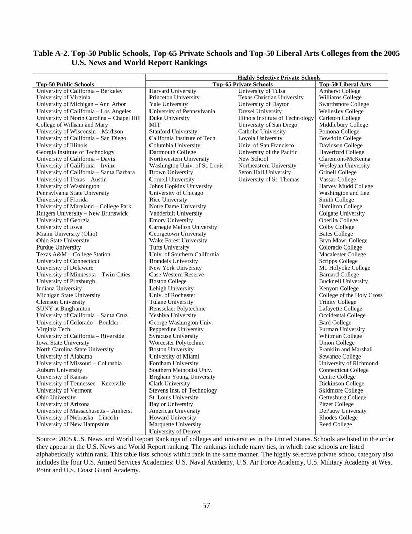
57

Table A-2. Top-50 Public Schools, Top-65 Private Schools and Top-50 Liberal Arts Colleges from the 2005 U.S. News and World Report Rankings

Source: 2005 U.S. News and World Report Rankings of colleges and universities in the United States. Schools are listed in the order they appear in the U.S. News and World Report ranking. The rankings include many ties, in which case schools are listed alphabetically within rank. This table lists schools within rank in the same manner. The highly selective private school category also includes the four U.S. Armed Services Academies: U.S. Naval Academy, U.S. Air Force Academy, U.S. Military Academy at West Point and U.S. Coast Guard Academy.

Highly Selective Private Schools Top-50 Public Schools Top-65 Private Schools Top-50 Liberal ArtsUniversity of California – Berkeley Harvard University University of Tulsa Amherst CollegeUniversity of Virginia Princeton University Texas Christian University Williams CollegeUniversity of Michigan – Ann Arbor Yale University University of Dayton Swarthmore CollegeUniversity of California – Los Angeles University of Pennsylvania Drexel University Wellesley CollegeUniversity of North Carolina – Chapel Hill Duke University Illinois Institute of Technology Carleton CollegeCollege of William and Mary MIT University of San Diego Middlebury CollegeUniversity of Wisconsin – Madison Stanford University Catholic University Pomona CollegeUniversity of California – San Diego California Institute of Tech. Loyola University Bowdoin CollegeUniversity of Illinois Columbia University Univ. of San Francisco Davidson CollegeGeorgia Institute of Technology Dartmouth College University of the Pacific Haverford CollegeUniversity of California – Davis Northwestern University New School Claremont-McKennaUniversity of California – Irvine Washington Univ. of St. Louis Northeastern University Wesleyan UniversityUniversity of California – Santa Barbara Brown University Seton Hall University Grinell CollegeUniversity of Texas – Austin Cornell University University of St. Thomas Vassar CollegeUniversity of Washington Johns Hopkins University Harvey Mudd CollegePennsylvania State University University of Chicago Washington and LeeUniversity of Florida Rice University Smith CollegeUniversity of Maryland – College Park Notre Dame University Hamilton CollegeRutgers University – New Brunswick Vanderbilt University Colgate UniversityUniversity of Georgia Emory University Oberlin CollegeUniversity of Iowa Carnegie Mellon University Colby CollegeMiami University (Ohio) Georgetown University Bates CollegeOhio State University Wake Forest University Bryn Mawr CollegePurdue University Tufts University Colorado CollegeTexas A&M – College Station Univ. of Southern California Macalester CollegeUniversity of Connecticut Brandeis University Scripps CollegeUniversity of Delaware New York University Mt. Holyoke CollegeUniversity of Minnesota – Twin Cities Case Western Reserve Barnard CollegeUniversity of Pittsburgh Boston College Bucknell UniversityIndiana University Lehigh University Kenyon CollegeMichigan State University Univ. of Rochester College of the Holy CrossClemson University Tulane University Trinity CollegeSUNY at Binghamton Rensselaer Polytechnic Lafayette CollegeUniversity of California – Santa Cruz Yeshiva University Occidental CollegeUniversity of Colorado – Boulder George Washington Univ. Bard CollegeVirginia Tech. Pepperdine University Furman UniversityUniversity of California – Riverside Syracuse University Whitman CollegeIowa State University Worcester Polytechnic Union CollegeNorth Carolina State University Boston University Franklin and MarshallUniversity of Alabama University of Miami Sewanee CollegeUniversity of Missouri – Columbia Fordham University University of RichmondAuburn University Southern Methodist Univ. Connecticut CollegeUniversity of Kansas Brigham Young University Centre CollegeUniversity of Tennessee – Knoxville Clark University Dickinson CollegeUniversity of Vermont Stevens Inst. of Technology Skidmore CollegeOhio University St. Louis University Gettysburg CollegeUniversity of Arizona Baylor University Pitzer CollegeUniversity of Massachusetts – Amherst American University DePauw UniversityUniversity of Nebraska – Lincoln Howard University Rhodes CollegeUniversity of New Hampshire Marquette University Reed College University of Denver

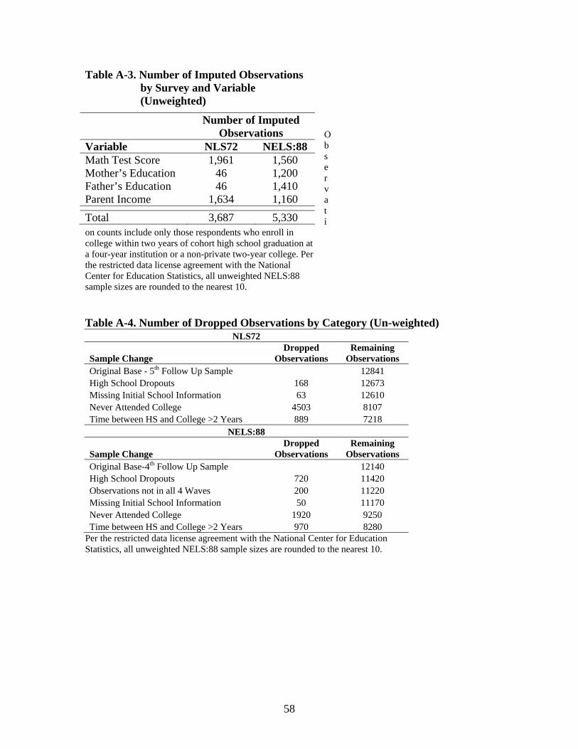
58

Table A-3. Number of Imputed Observations by Survey and Variable (Unweighted)

Observati

on counts include only those respondents who enroll in college within two years of cohort high school graduation at a four-year institution or a non-private two-year college. Per the restricted data license agreement with the National Center for Education Statistics, all unweighted NELS:88 sample sizes are rounded to the nearest 10. Table A-4. Number of Dropped Observations by Category (Un-weighted)

NLS72

Sample Change Dropped

Observations Remaining

Observations Original Base - 5th Follow Up Sample 12841 High School Dropouts 168 12673 Missing Initial School Information 63 12610 Never Attended College 4503 8107 Time between HS and College >2 Years 889 7218

NELS:88

Sample Change Dropped

Observations Remaining

Observations Original Base-4th Follow Up Sample 12140 High School Dropouts 720 11420 Observations not in all 4 Waves 200 11220 Missing Initial School Information 50 11170 Never Attended College 1920 9250 Time between HS and College >2 Years 970 8280

Per the restricted data license agreement with the National Center for Education Statistics, all unweighted NELS:88 sample sizes are rounded to the nearest 10.

Number of Imputed Observations

Variable NLS72 NELS:88 Math Test Score 1,961 1,560 Mother’s Education 46 1,200 Father’s Education 46 1,410 Parent Income 1,634 1,160

Total 3,687 5,330

59

Appendix B: Supplemental Decomposition Tables Table B-1. Decompositions Using Average Derivatives From Logit Models of College Completion in the NELS:88 Survey by

Type of Institution

Full

Sample

Public Non-Top

50 Public Top 50

Private Less

Selective

Private Highly

Selective Community

College NLS72 50.5 61.8 73.5 58.2 80.1 20.2

NELS:88 45.9 56.9 82.5 70.5 90.3 17.6 Total Change -4.6 -4.9 9.0 12.3 10.3 -2.5

Change Due to Observables (X) -4.0 -1.7 3.4 3.0 6.5 -3.5 Change Due to Student Characteristics -0.4 2.1 2.8 3.6 6.3 -3.0 Math Test Percentiles -1.6 0.1 1.0 0.2 0.4 -2.6 Other Student Characteristics 1.2 2.0 1.8 3.4 5.9 -0.4 Change Due to Supply-Side Factors -3.6 -3.8 0.6 -0.6 0.2 -0.5 Student-Faculty Ratios -1.2 -3.8 0.6 -0.6 0.2 -0.5 Initial School Types -2.4

Residual -0.6 -3.2 5.6 9.3 3.8 1.0 a Source: Authors’ calculations as described in the text from the NLS72 and NELS:88 surveys . NLS72 calculations were made using the fifth follow-up weights included

in the survey. Fourth follow-up weights were used for the NELS:88 survey calculations. Only those participating in these follow-ups are included in the regression. School type samples refer to first institution attended. The NLS72 and NELS:88 samples are restricted to those who attend college within 2 years of cohort high school graduation. Cohort high school graduation is defined as June 1972 for the NLS72 sample and June 1992 for the NELS:88 sample.

b All decompositions are computed using average marginal effects from logit models of completion likelihood estimated with the NELS:88 data as described in the main text. Simulated changes are calculated by multiplying the average marginal effect for a given variable by the observed change in means across surveys.

c The Change Due to Observables is the difference between the observed NELS:88 completion rate and the simulated NELS:88 completion rate using the distribution of all observables from NLS72. The changes due to math test percentiles, student-faculty ratios and initial school types are the differences between the observed NELS:88 completion rate and the simulated NELS:88 completion rates in which we simulate the completion rate if the each variable were distributed as in the NLS72 survey and all other observables were unchanged. The Change Due to Supply Side Factors is the sum of the changes due to student-faculty ratios and initial school types. We calculate the Change Due to Student Characteristics as the difference between the Change Due to Observables (X) and the Change Due to Supply-Side Factors. The Change Due to Other Student Characteristics is calculated by subtracting the Change Due to Math Test Percentiles from the Change Due to Student Characteristics.

d Data on faculty and enrollment are from the HEGIS/IPEDS surveys from the Department of Education.

60

Table B-2. Decompositions Using Average Derivatives From Logit Models of College Completion in the NELS:88 Survey by Type of

Institution and Gender Panel A: Men

Full Sample

Public Non-Top

50 Public Top 50

Private Less

Selective

Private Highly

Selective Community

College NLS72 51.7 61.2 73.8 59.9 82.7 21.6 NELS:88 43.2 51.6 77.5 67.7 89.2 17.7 Total Change -8.5 -9.6 3.7 7.8 6.5 -3.9

Change Due to Observables (X) -5.4 -2.1 1.9 1.1 7.1 -3.6 Change Due to Student Characteristics -1.2 1.5 1.3 1.5 6.6 -3.0 Math Test Percentiles -2.5 -0.7 0.6 -1.9 0.4 -3.1 Other Student Characteristics 1.3 2.2 0.7 3.4 6.2 0.1 Change Due to Supply-Side Factors -4.2 -3.6 0.6 -0.4 0.5 -0.6 Student-Faculty Ratios -1.3 -3.6 0.6 -0.4 0.5 -0.6 Initial School Types -2.9

Residual -3.1 -7.5 1.8 6.7 -0.6 -0.3

61

Panel B: Women

Full Sample

Public Non-Top

50 Public Top 50

Private Less

Selective

Private Highly

Selective Community

College NLS72 49.2 62.4 73.1 56.5 75.6 18.6 NELS:88 48.5 61.8 87.7 72.6 91.4 17.5 Total Change -0.8 -0.6 14.6 15.9 15.8 -1.1

Change Due to Observables (X) -2.8 -1.4 3.5 4.3 5.3 -3.5 Change Due to Student Characteristics 0.2 2.4 2.9 5.1 5.3 -3.0 Math Test Percentiles -0.6 1.0 1.4 2.1 0.5 -2.0 Other Student Characteristics 0.8 1.4 1.5 3.0 4.8 -1.0 Change Due to Supply-Side Factors -3.0 -3.8 0.6 -0.8 0.0 -0.5 Student-Faculty Ratios -1.2 -3.8 0.6 -0.8 0.0 -0.5 Initial School Types -1.8

Residual 2.0 0.8 11.1 11.6 10.5 2.4 a Source: Authors’ calculations as described in the text from the NLS72 and NELS:88 surveys . NLS72 calculations were made using the fifth follow-up weights included

in the survey. Fourth follow-up weights were used for the NELS:88 survey calculations. Only those participating in these follow-ups are included in the regression. School type samples refer to first institution attended. The NLS72 and NELS:88 samples are restricted to those who attend college within 2 years of cohort high school graduation. Cohort high school graduation is defined as June 1972 for the NLS72 sample and June 1992 for the NELS:88 sample.

b All decompositions are computed using average marginal effects from logit models of completion likelihood estimated with the NELS:88 data as described in the main text. Simulated changes are calculated by multiplying the average marginal effect for a given variable by the observed change in means across surveys.

c The Change Due to Observables is the difference between the observed NELS:88 completion rate and the simulated NELS:88 completion rate using the distribution of all observables from NLS72. The changes due to math test percentiles, student-faculty ratios and initial school types are the differences between the observed NELS:88 completion rate and the simulated NELS:88 completion rates in which we simulate the completion rate if the each variable were distributed as in the NLS72 survey and all other observables were unchanged. The Change Due to Supply Side Factors is the sum of the changes due to student-faculty ratios and initial school types. We calculate the Change Due to Student Characteristics as the difference between the Change Due to Observables (X) and the Change Due to Supply-Side Factors. The Change Due to Other Student Characteristics is calculated by subtracting the Change Due to Math Test Percentiles from the Change Due to Student Characteristics.

d Data on faculty and enrollment are from the HEGIS/IPEDS surveys from the Department of Education.

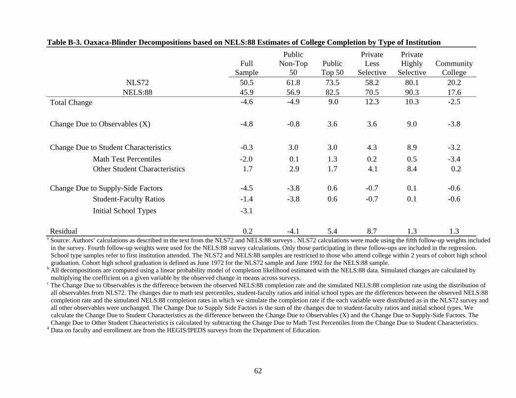
62

Table B-3. Oaxaca-Blinder Decompositions based on NELS:88 Estimates of College Completion by Type of Institution

Full

Sample

Public Non-Top

50 Public Top 50

Private Less

Selective

Private Highly

Selective Community

College NLS72 50.5 61.8 73.5 58.2 80.1 20.2

NELS:88 45.9 56.9 82.5 70.5 90.3 17.6 Total Change -4.6 -4.9 9.0 12.3 10.3 -2.5

Change Due to Observables (X) -4.8 -0.8 3.6 3.6 9.0 -3.8 Change Due to Student Characteristics -0.3 3.0 3.0 4.3 8.9 -3.2 Math Test Percentiles -2.0 0.1 1.3 0.2 0.5 -3.4 Other Student Characteristics 1.7 2.9 1.7 4.1 8.4 0.2 Change Due to Supply-Side Factors -4.5 -3.8 0.6 -0.7 0.1 -0.6 Student-Faculty Ratios -1.4 -3.8 0.6 -0.7 0.1 -0.6 Initial School Types -3.1

Residual 0.2 -4.1 5.4 8.7 1.3 1.3 a Source: Authors’ calculations as described in the text from the NLS72 and NELS:88 surveys . NLS72 calculations were made using the fifth follow-up weights included

in the survey. Fourth follow-up weights were used for the NELS:88 survey calculations. Only those participating in these follow-ups are included in the regression. School type samples refer to first institution attended. The NLS72 and NELS:88 samples are restricted to those who attend college within 2 years of cohort high school graduation. Cohort high school graduation is defined as June 1972 for the NLS72 sample and June 1992 for the NELS:88 sample.

b All decompositions are computed using a linear probability model of completion likelihood estimated with the NELS:88 data. Simulated changes are calculated by multiplying the coefficient on a given variable by the observed change in means across surveys.

c The Change Due to Observables is the difference between the observed NELS:88 completion rate and the simulated NELS:88 completion rate using the distribution of all observables from NLS72. The changes due to math test percentiles, student-faculty ratios and initial school types are the differences between the observed NELS:88 completion rate and the simulated NELS:88 completion rates in which we simulate the completion rate if the each variable were distributed as in the NLS72 survey and all other observables were unchanged. The Change Due to Supply Side Factors is the sum of the changes due to student-faculty ratios and initial school types. We calculate the Change Due to Student Characteristics as the difference between the Change Due to Observables (X) and the Change Due to Supply-Side Factors. The Change Due to Other Student Characteristics is calculated by subtracting the Change Due to Math Test Percentiles from the Change Due to Student Characteristics.

4 Data on faculty and enrollment are from the HEGIS/IPEDS surveys from the Department of Education.

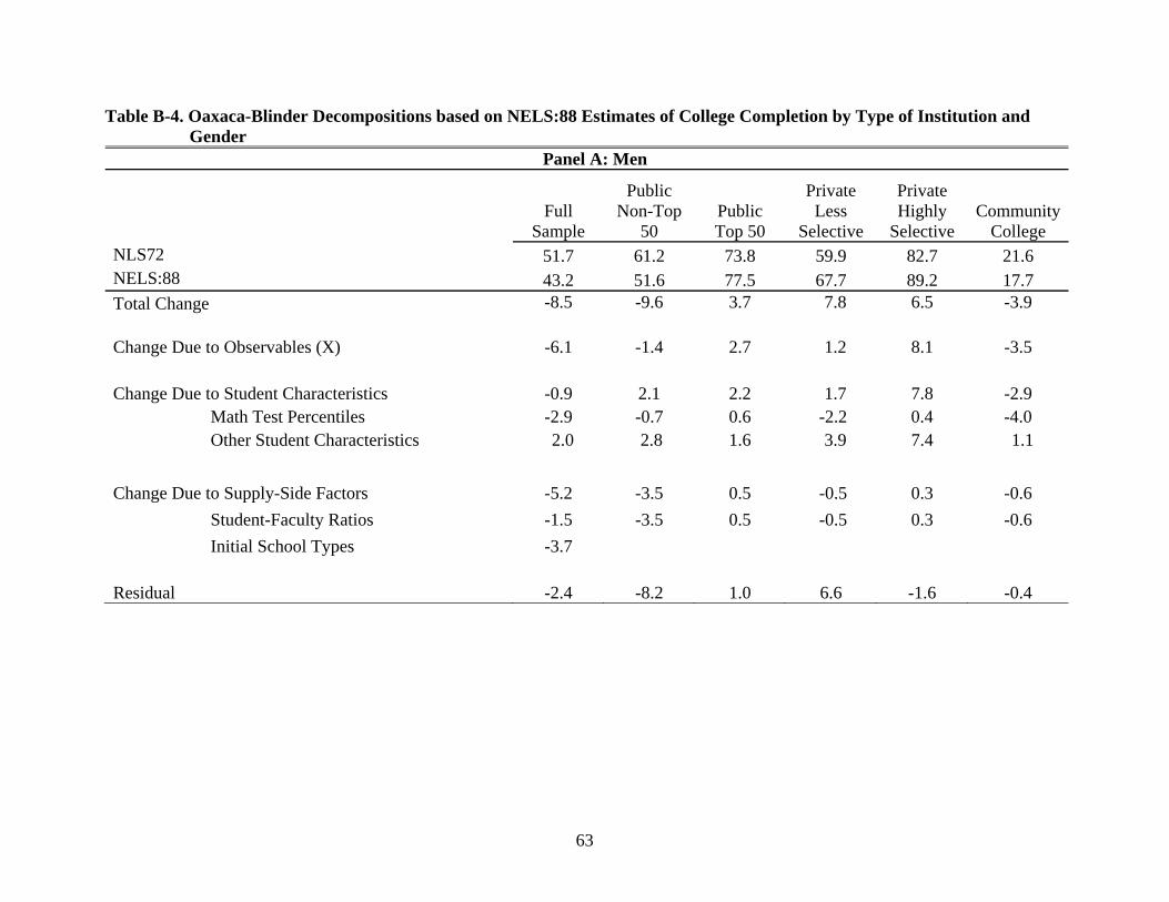
63

Table B-4. Oaxaca-Blinder Decompositions based on NELS:88 Estimates of College Completion by Type of Institution and

Gender Panel A: Men

Full Sample

Public Non-Top

50 Public Top 50

Private Less

Selective

Private Highly

Selective Community

College NLS72 51.7 61.2 73.8 59.9 82.7 21.6 NELS:88 43.2 51.6 77.5 67.7 89.2 17.7 Total Change -8.5 -9.6 3.7 7.8 6.5 -3.9

Change Due to Observables (X) -6.1 -1.4 2.7 1.2 8.1 -3.5 Change Due to Student Characteristics -0.9 2.1 2.2 1.7 7.8 -2.9 Math Test Percentiles -2.9 -0.7 0.6 -2.2 0.4 -4.0 Other Student Characteristics 2.0 2.8 1.6 3.9 7.4 1.1 Change Due to Supply-Side Factors -5.2 -3.5 0.5 -0.5 0.3 -0.6 Student-Faculty Ratios -1.5 -3.5 0.5 -0.5 0.3 -0.6 Initial School Types -3.7

Residual -2.4 -8.2 1.0 6.6 -1.6 -0.4

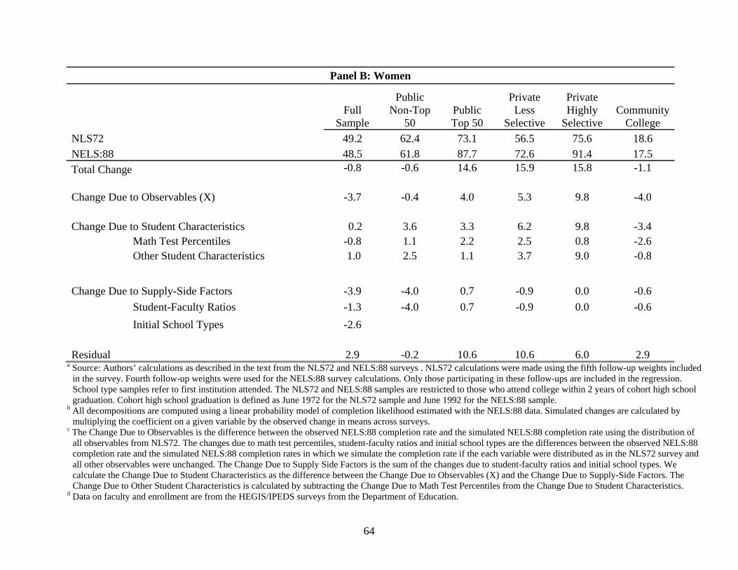
64

Panel B: Women

Full Sample

Public Non-Top

50 Public Top 50

Private Less

Selective

Private Highly

Selective Community

College NLS72 49.2 62.4 73.1 56.5 75.6 18.6 NELS:88 48.5 61.8 87.7 72.6 91.4 17.5 Total Change -0.8 -0.6 14.6 15.9 15.8 -1.1

Change Due to Observables (X) -3.7 -0.4 4.0 5.3 9.8 -4.0 Change Due to Student Characteristics 0.2 3.6 3.3 6.2 9.8 -3.4 Math Test Percentiles -0.8 1.1 2.2 2.5 0.8 -2.6 Other Student Characteristics 1.0 2.5 1.1 3.7 9.0 -0.8 Change Due to Supply-Side Factors -3.9 -4.0 0.7 -0.9 0.0 -0.6 Student-Faculty Ratios -1.3 -4.0 0.7 -0.9 0.0 -0.6 Initial School Types -2.6

Residual 2.9 -0.2 10.6 10.6 6.0 2.9 a Source: Authors’ calculations as described in the text from the NLS72 and NELS:88 surveys . NLS72 calculations were made using the fifth follow-up weights included

in the survey. Fourth follow-up weights were used for the NELS:88 survey calculations. Only those participating in these follow-ups are included in the regression. School type samples refer to first institution attended. The NLS72 and NELS:88 samples are restricted to those who attend college within 2 years of cohort high school graduation. Cohort high school graduation is defined as June 1972 for the NLS72 sample and June 1992 for the NELS:88 sample.

b All decompositions are computed using a linear probability model of completion likelihood estimated with the NELS:88 data. Simulated changes are calculated by multiplying the coefficient on a given variable by the observed change in means across surveys.

c The Change Due to Observables is the difference between the observed NELS:88 completion rate and the simulated NELS:88 completion rate using the distribution of all observables from NLS72. The changes due to math test percentiles, student-faculty ratios and initial school types are the differences between the observed NELS:88 completion rate and the simulated NELS:88 completion rates in which we simulate the completion rate if the each variable were distributed as in the NLS72 survey and all other observables were unchanged. The Change Due to Supply Side Factors is the sum of the changes due to student-faculty ratios and initial school types. We calculate the Change Due to Student Characteristics as the difference between the Change Due to Observables (X) and the Change Due to Supply-Side Factors. The Change Due to Other Student Characteristics is calculated by subtracting the Change Due to Math Test Percentiles from the Change Due to Student Characteristics.

d Data on faculty and enrollment are from the HEGIS/IPEDS surveys from the Department of Education.