
WHY ARE LATIN AMERICANS SO UNHAPPY ABOUT ...
395
Journal of Applied Economics, Vol. VIII, No. 1 (May 2005), 1-29 WHY ARE LATIN AMERICANS SO UNHAPPY ABOUT REFORMS? UGO PANIZZA AND MONICA YAÑEZ * Inter-American Development Bank Submitted November 2003; accepted May 2004 This paper uses opinion surveys to document discontent with the pro-market reforms implemented by most Latin American countries during the 1990s. The paper also explores four possible sets of explanations for this discontent: (i) a general drift of the populace’s political views to the left; (ii) an increase in political activism by those who oppose reforms; (iii) a decline in the people’s trust of political actors; and (iv) the economic crisis. The paper’s principal finding is that the macroeconomic situation plays an important role in explaining the dissatisfaction with the reform process. JEL classification codes: P16, O54 Key words: political economy, reforms; crisis, Latin America I. Introduction There is by now a large body of literature that describes and discusses the discontent with the pro-market reforms commonly referred to as the “Washington Consensus” (Williamson, 1990), and often associated with the process of “Globalization” (for a survey, see Lora and Panizza, 2003; and Stiglitz, 2002). The objective of this paper is to use opinion polls to document Latin Americans’ increasing discontent with those reforms and to explore * Ugo Panizza (corresponding author) and Monica Yañez: Research Department, Inter- American Development Bank, 1300 New York Ave., NW, Washington, DC 20577, USA. Tel (202) 623-1000; E-mail: [email protected] and [email protected]. We would like to thank Eduardo Lora, Jorge Streb, and three anonymous referees for very helpful comments, and John Smith and Tim Duffy for expert editing. The views expressed in this paper are the authors’ and do not necessarily reflect those of the Inter-American Development Bank. The usual caveats apply.
-
Upload
khangminh22 -
Category
Documents
-
view
1 -
download
0
Transcript of WHY ARE LATIN AMERICANS SO UNHAPPY ABOUT ...
1WHY ARE LATIN AMERICANS SO UNHAPPY ABOUT REFORMS?Journal of Applied Economics, Vol. VIII, No. 1 (May 2005), 1-29
WHY ARE LATIN AMERICANSSO UNHAPPY ABOUT REFORMS?
UGO PANIZZA AND MONICA YAÑEZ *
Inter-American Development Bank
Submitted November 2003; accepted May 2004
This paper uses opinion surveys to document discontent with the pro-market reformsimplemented by most Latin American countries during the 1990s. The paper also exploresfour possible sets of explanations for this discontent: (i) a general drift of the populace’spolitical views to the left; (ii) an increase in political activism by those who oppose reforms;(iii) a decline in the people’s trust of political actors; and (iv) the economic crisis. Thepaper’s principal finding is that the macroeconomic situation plays an important role inexplaining the dissatisfaction with the reform process.
JEL classification codes: P16, O54
Key words: political economy, reforms; crisis, Latin America
I. Introduction
There is by now a large body of literature that describes and discusses the
discontent with the pro-market reforms commonly referred to as the
“Washington Consensus” (Williamson, 1990), and often associated with the
process of “Globalization” (for a survey, see Lora and Panizza, 2003; and
Stiglitz, 2002). The objective of this paper is to use opinion polls to document
Latin Americans’ increasing discontent with those reforms and to explore
* Ugo Panizza (corresponding author) and Monica Yañez: Research Department, Inter-American Development Bank, 1300 New York Ave., NW, Washington, DC 20577, USA.Tel (202) 623-1000; E-mail: [email protected] and [email protected]. We would like tothank Eduardo Lora, Jorge Streb, and three anonymous referees for very helpful comments,and John Smith and Tim Duffy for expert editing. The views expressed in this paper are theauthors’ and do not necessarily reflect those of the Inter-American Development Bank.The usual caveats apply.

2 JOURNAL OF APPLIED ECONOMICS
possible explanations for this trend. We evaluate four possible explanations
for this dissatisfaction. The first focuses on a change in political orientation.
The second focuses on a change in political activism on the part of those who
oppose reforms. The third focuses on trust in political actors. The fourth
focuses on the economic situation. There is also an important set of
explanations for discontent with reforms that we do not consider in this paper.
This set of explanations focuses on the role of cognitive biases in the formation
of public opinion. An interesting paper by Pernice and Sturzenegger (2003)
studies the case of Argentina and uses cognitive bias (especially confirmatory
and self-serving biases) to explain rejection of reforms.
The paper is organized as follows. Section II describes some indicators
aimed at measuring support for pro-market reforms and describes their
evolution over time. It also describes the demographics of those who support
and oppose reforms. Section III explores possible explanations for discontent
with the reform process. Section IV concludes.
II. What Do Latin Americans Think of Reforms?
The purpose of this section is to gauge the attitude of Latin Americans
toward pro-market reforms. In order to do so, we use individual-level data
from the Latinobarómetro annual surveys. This data set covers 17 Latin
American countries over a period of 7 years (1996-2003) and consists of an
average of 1,200 respondents per country-year.1 A Latinobarómetro survey
was conducted in 1995, but we have excluded it because it covers a smaller
set of countries. Data for the 2002 survey were not made available to us and
hence are not included in the analysis. National polling firms in each individual
country conduct the surveys, so the sampling method from country to country
varies slightly. However, in most cases the selection includes some quotas to
ensure representation across gender, socio-economic status, and age.
Although the Latinobarómetro data offer an unprecedented wealth of
information, some problems with the survey do exist. The first is that the
1 The surveyed countries are: Argentina, Bolivia, Brazil, Chile, Colombia, Costa Rica,Ecuador, El Salvador, Guatemala, Honduras, Mexico, Nicaragua, Panama, Peru, Paraguay,Uruguay, and Venezuela.

3WHY ARE LATIN AMERICANS SO UNHAPPY ABOUT REFORMS?
Latinobarómetro survey initially focused exclusively on the urban population.
While most of the recent surveys have national coverage and samples
representing the whole population, in Chile, Colombia and Paraguay the
coverage is only urban (the urban populations are 70 percent, 51 percent, and
30 percent of the total population). Second, until 2002, the surveys were
conducted using only the country’s official language (Spanish or Portuguese);
consequently, were not representative of the attitudes of those portions of the
indigenous population that are not fluent in the official language. Moreover,
there is some evidence that, at least in the early years, the pool of survey
respondents over-represented individuals with relatively high levels of
education (Gaviria, Panizza, and Seddon, 2004). Finally, the survey does not
ask directly about pro-market reforms. Therefore, while it would be most
desirable to have a set of variables that directly measure Latin Americans’
opinion toward pro-market reforms, we must use the available variables to
build several indicators to serve as a reasonable proxy. The reader should
keep in mind that some of our variables better proxy opinions toward reforms
while others better proxy opinions toward market economy.2
Our preferred variable is PRIVAT (available for 1998, 2000, 2001, and
2003) which takes value one if the respondent thinks that the privatization
process benefited the country and zero otherwise. Among our variables, this
is probably the most accurate measure of opinion of one type of reform that
was prevalent in most Latin American countries. A second set of variables
measures the general attitude toward the market economy. MARKET
(available for 1998 and 2000) takes value one if the respondent thinks that a
market economy is good for the country and zero otherwise. PRICES (available
for 1998, 2000, and 2001) takes a value of one if the respondent thinks that
prices should be set by the market and zero if prices should be decided by
some central authority. PRIVPROD (available for 1998 and 2001) takes a
value of one if the respondent thinks that productive activity should be left to
the private sector and zero otherwise. It should be clear that MARKET,
PRICES and PRIVPROD are direct measures of the public’s attitude toward
a market economy . They can be used as a proxy for Latin Americans’ position
2 Table A1 provides the detailed information about the questions used to build the variables.

4 JOURNAL OF APPLIED ECONOMICS
toward reforms only by assuming that the main aim of the structural reform
process was liberalizing the economy. We do not find such an assumption
unrealistic. In fact, five of the ten original points in Williamson’s (1990)
“Washington Consensus” focused on expanding the role of the market
economy.
The third set of indicators deals with attitudes towards international trade
and foreign direct investment. LACINT (available for 1996, 1997, 1998, and
2001) is a dichotomous variable that takes a value of one if the respondent
holds a favorable view of economic integration in Latin America and a value
of zero if the respondent is against the integration process. This is probably
the most problematic variable. As individuals who are against economic
reforms and free trade in general might still favor Latin American integration,
it is a very imperfect proxy of attitudes toward free trade (which, ideally, is
what we want to measure). In fact, Table A2 in the Appendix shows a very
low correlation of LACINT with most of the other variables used in this paper.3
Therefore, all results concerning LACINT should be interpreted with some
caution.
FDI takes value one if the respondent thinks that foreign direct investment
is beneficial for the country and zero if foreign direct investment is harmful.
We think that FDI is a good measure of at least one aspect of the reforms
process (i.e., opening the economy to foreign investors). The main problem
with this variable is that it is only available for one year (1998), thus it is
impossible to track its evolution over time.
Table 1 summarizes the average values of the five variables mentioned
above. The most striking number is the large drop in support for privatization
(FDI has no time variation). In 1998, more than 50 percent of Latin Americans
thought that privatization was beneficial for their country. This percentage
dropped to 31 percent in 2001 and to 25 percent in 2003. We observe a similar
trend for MARKET. In 1998, 77 percent of Latin Americans thought that a
market economy was good for the country. In 2000, the percentage supporting
3 We would like to thank an anonymous referee for pointing this out and suggesting that“Latin American integration is throughout the Region a value cherished by all kinds ofleftists and nationalists who oppose economic reforms.”

5WHY ARE LATIN AMERICANS SO UNHAPPY ABOUT REFORMS?
Table 1. What Do Latin Americans Think of Pro-Market Reforms?
LACINT FDI PRIVAT MARKET PRICES PRIVPROD
1996 0.74 --- --- --- --- ---
1997 0.87 --- --- --- --- ---
1998 0.88 0.77 0.52 0.77 0.63 0.56
2000 --- --- 0.38 0.67 0.57 ---
2001 0.84 --- 0.31 --- 0.59 0.50
2003 --- --- 0.25 --- --- ---
Note: The values reported in the table measure the share of respondents that support LatinAmerican economic integration, FDI, privatization, market economy, price liberalizationand private production.
a market economy dropped to 67 percent.4 Support for private production
and market prices also dropped, but by a smaller amount, and there was no
change in support for economic integration in Latin America. Table A2 in the
Appendix shows that the correlation between these variables, while positive
and statistically significant, is rather low, which indicates that the different
questions do in fact capture different aspects of attitudes toward pro-market
reforms.
It is worth mentioning that, while over the period that goes from 1985 to
1995 most Latin American countries implemented extensive pro-market
reforms, the reform process has not been homogenous across countries and
across types of reforms (Lora and Panizza, 2003; and Lora and Olivera,
2004a,b). Although these considerations suggest that it may be misleading to
talk of Latin America as a homogenous entity, it is worth mentioning that the
4 Unfortunately, a change in the questionnaire made it impossible to look at the behavior ofthis question in 2003. The surveys from 1998 and 2000 asked: “Do you think that a marketeconomy is good for the country?” For the year 2003, the question was: “Are you satisfiedwith the functioning of the market economy?” Only 18 percent of respondents gave anaffirmative answer to this question. Notice that the evolution of the various indicators isnot driven by the extreme behavior of Argentina. We obtain similar results even afterdropping Argentina from the sample. For instance, support for privatization would gofrom 52 percent (in 1998) to 26 percent (in 2003).

6 JOURNAL OF APPLIED ECONOMICS
0 0,1 0,2 0,3 0,4 0,5 0,6 0,7
PAN
UR Y
COL
AR G
PER
NIC
B R A
CHI
ELS
MEX
PR Y
ECU
B OL
HON
VEN
GT M
1998 2003
Figure 1. Support for Privatization*
Note: *Share of respondents who think that privatizations have been beneficial for thecountry.
drop in support for privatization was general. As Figure 1 shows, in ten out of
sixteen countries in 1998, more than 50 percent of survey respondents supported
privatization. In 2003, there was no country in which a majority of the
population supported privatization. Support for privatization in 2003 ranged
from 37 percent (in Brazil) to just above 10 percent (in Argentina and Panama).
Argentina, Bolivia, Ecuador, El Salvador, Guatemala, and Paraguay are the
countries where support for privatization dropped by the largest amount.
Before attempting to explain the drop in support for pro-market reforms and
the market economy, it is interesting to look at the demographics of those who
support and oppose reforms. We do so by running a set of regressions in which
the dependent variables are the different indicators used to measure attitude
toward reforms and the explanatory variables include a set of demographic and
socio-economic variables that include respondents’ age, sex, education,
wealth, socioeconomic status and happiness/optimism (Table 2). To make
the results more intuitive, regressions were estimated using a linear

7WHY ARE LATIN AMERICANS SO UNHAPPY ABOUT REFORMS?
Table 2. Attitude Toward Reforms by Socioeconomic Characteristics
(1) (2) (3) (4) (5) (6)
LACINT FDI PRIVAT MARKET PRICES PRIVPROD
HAPPY 12.047 18.066 32.227 22.978 15.570 7.591
(5.02)*** (2.60)** (9.75)*** (4.55)*** (4.17)*** (1.78)*
AGE 0.085 0.128 -0.194 -0.008 0.017 0.472
(0.89) (0.65) (2.02)* (0.09) (0.15) (3.19)***
AGE2 -0.000 -0.001 0.002 0.001 0.000 -0.004
(0.33) (0.56) (1.59) (0.58) (0.37) (2.72)**
SEX -1.201 -5.366 -1.615 -1.667 -3.899 -4.091
(3.00)*** (4.10)*** (3.10)*** (3.75)*** (4.92)*** (4.56)***
quintile==2 1.745 3.128 -1.314 -1.457 -0.333 -0.612
(2.34)** (1.98)* (2.06)* (1.24) (0.36) (0.59)
quintile==3 3.256 4.328 -0.978 0.945 1.682 0.307
(5.18)*** (2.59)** (0.97) (0.62) (1.83)* (0.20)
quintile==4 3.452 7.502 -0.632 0.346 2.464 1.574
(3.99)*** (3.10)*** (0.71) (0.26) (2.91)** (1.07)
quintile==5 4.023 10.291 2.568 2.676 4.810 5.039
(4.54)*** (5.64)*** (2.11)* (1.80)* (3.30)*** (2.62)**
EDUCA==2 1.622 1.651 -2.560 2.562 1.971 -0.395
(1.38) (0.62) (1.88)* (0.98) (1.49) (0.19)
EDUCA==3 3.283 4.896 -3.529 2.351 2.036 -1.427
(2.61)** (2.04)* (2.12)* (1.17) (1.16) (0.58)
EDUCA==4 4.625 6.024 -4.666 3.392 2.234 -1.359
(3.57)*** (2.90)** (2.92)** (1.63) (1.83)* (0.64)
EDUCA==5 5.295 8.026 -3.546 3.708 3.116 -1.920
(3.74)*** (3.63)*** (1.92)* (1.41) (2.20)** (0.72)
EDUCA==6 7.644 8.956 -2.772 1.274 2.244 -2.201
(6.21)*** (3.57)*** (1.51) (0.48) (1.21) (0.87)
EDUCA==7 7.289 10.921 0.526 2.726 3.343 1.145
(5.26)*** (4.40)*** (0.25) (1.08) (1.77)* (0.47)
SOC_EC==1 1.027 1.598 -1.437 -0.557 -1.786 -0.006
(1.00) (0.75) (1.08) (0.32) (1.49) (0.00)

8 JOURNAL OF APPLIED ECONOMICS
SOC_EC==2 1.949 0.400 -1.437 1.381 -1.375 -2.004
(1.54) (0.19) (1.22) (0.62) (1.23) (0.94)
SOC_EC==3 3.021 -0.655 -0.712 2.295 -0.626 -1.447
(2.11)* (0.22) (0.53) (0.92) (0.47) (0.71)
SOC_EC==4 3.555 2.571 2.049 3.191 1.673 2.366
(1.98)* (0.87) (1.28) (0.88) (1.27) (1.03)
Constant 69.614 47.351 37.726 49.178 58.990 40.082
(25.04)*** (7.23)*** (12.97)*** (11.45)*** (20.75)*** (7.89)***
Observations 55080 11508 60721 26207 44110 28010
R-squared 0.07 0.07 0.09 0.05 0.04 0.04
Notes: All the equations are estimated using a linear probability model and include country-year fixed effects and country-year clustered standard errors. Robust t statistics inparentheses. * significant at 10%; ** significant at 5%; *** significant at 1%. Education isproxied with 7 dummies variables: 1 indicates illiterate, 2 indicates some primary, 3 indicatescompleted primary, 4 indicates some secondary, 5 indicates completed secondary, 6 indicatessome university, and 7 indicates completed university. Illiterate is the excluded dummy.The wealth quintiles (quintile) were built as the principal component of several indicatorsof asset ownership. The variable measuring happiness/optimism (HAPPY) was built as theprincipal component of three questions focusing on whether the respondent is satisfiedwith his/her life and on how he/she evaluates his/her current and future economic situation.The SEX variable takes value 0 for men and value 1 for women. More details are providedin Table A1.
Table 2. (Continued) Attitude Toward Reforms By SocioeconomicCharacteristics
(1) (2) (3) (4) (5) (6)
LACINT FDI PRIVAT MARKET PRICES PRIVPROD
probability model.5 All regressions include country-fixed effects and country-
specific time effects, and the standard errors are clustered by country-year.
In all cases, we find that men tend to be more supportive of pro-market
reforms than women. The difference ranges from one percentage point in the
case of LACINT to five percentage points in the case of FDI. The estimations
5 Probit estimations (available upon request) yield similar results.

9WHY ARE LATIN AMERICANS SO UNHAPPY ABOUT REFORMS?
suggest that there is a positive correlation between happiness/optimism (as
measured by the variable HAPPY) and support for reform and free markets.
Quantitatively, the effect of happiness is very important. An individual who
claims to be very happy (HAPPY = 1) is between 8 and 32 percentage points
more likely to support reforms than an individual who claims to be very
unhappy (HAPPY = 0). In the case of privatization, a one standard deviation
increase in happiness (equivalent to 0.16 points in the happiness index) is
associated to a 5.15 percentage point increase in support for privatization. No
other respondent-specific variable has a quantitatively similar effect on support
for reform.
We also find that support for economic integration (measured by LACINT
and FDI) increases with wealth and education. The effect of education is
particularly strong for LACINT and FDI.6 In the case of PRIVAT, we find
that wealth is rarely statistically significant and that individuals with
intermediate levels of education are strongly opposed to privatization. The
coefficient of education in the PRIVAT variable is almost always negative;
the only exception is for individuals who have completed university. Education
is positively correlated with MARKET and PRICES and negatively correlated
with PRIVPROD, but the coefficients are rarely statistically significant.
Wealth, instead, is positively correlated with these variables. In particular,
the regressions indicate that individuals belonging to the top quintile of the
wealth distribution show a strong support for the market economy, liberalized
prices, and private production.
Finally, the regressions also include a variable measuring the respondent’s
socio-economic status (SOC_EC measures socio economic status as judged
by the interviewer, a higher value indicates higher socio-economic status).
This variable is never statistically significant.
6 This is an interesting finding, because, according to standard trade theory, it is the relativelyabundant factor of production (unskilled labor, in the case of Latin America) that is likelyto receive the greatest benefit from economic integration. However, it bears repeating thatLACINT might be a poor proxy for the public’s overall attitude towards free trade. Analternative explanation is that, in the case of Latin America, skilled workers (rather thanunskilled) benefited more from trade and capital account liberalization (we would like tothank an anonymous referee for pointing this out).

10 JOURNAL OF APPLIED ECONOMICS
III. Reasons for the Discontent
The purpose of this section is to analyze possible explanations of the
discontent with the reform process. While there is extensive literature studying
the factors that drive the reform process and reform reversals, most of the
models emphasized in this literature are based on the behavior of political
parties and interest groups. To the best of our knowledge, there is no formal
model to analyze a sudden opinion change among the majority of a country’s
residents. Therefore, rather than basing our analysis on a formal model, we
list a series of hypotheses which are often put forward in policy circles and
analyze whether any of these hypotheses can explain the trends documented
in the previous section. In particular, we analyze four possible explanations:
(i) an overall movement of the population’s politics to the left; (ii) an increase
in political activism among reform opponents; (iii) a decline in the public’s
trust of political actors; and (iv) the economic crisis.
A. Have Latin Americans Moved to the Left?
One possible cause for the decrease in support for pro-market reforms
might be a general movement of the Latin American population toward the
political left. This could be part of a global trend generated by the end of the
Reagan-Thatcher era and the beginning of a worldwide movement toward
the left following, with a lag, the leadership of Bill Clinton and Tony Blair.
Latinobarómetro permits the investigation of this hypothesis because it
includes a question about the respondents’ political orientation. The question
asks: “On a scale of 0 to 10, how right wing are you?” with 0 being the
farthest left and 10 the farthest right. Figure 2 shows the average values for
all Latin American countries included in Latinobarómetro for 1996, 1998,
2001, and 2003. Each bar presents the share of respondents that declared
themselves in a given position on the political scale in a given year. The data
suggest that there has been no net change in political orientation which, if
anything, shows a small movement to the right.
If we focus on the behavior of extremists (left-wing extremists are defined
as those that chose values 0 or 1, and right-wing extremists are defined as
those who chose 9 or 10), we find that most Central American and Andean

11WHY ARE LATIN AMERICANS SO UNHAPPY ABOUT REFORMS?
countries are characterized by a large share of right-wing extremists.
Nicaragua, Panama, Venezuela, and Brazil are the most polarized countries,
with a significant segment of the population defining themselves as either
right-wing or left-wing extremist.7 At the same time, Argentina, Bolivia, and
Chile are the countries with the smallest share of extremists. While these
cross-country differences could be due to the fact that the definition of being
right-wing is country-specific,8 what is most important for our purposes is
the relative stability of political opinion, which provides prima facie evidence
that Latin Americans have not moved toward the political left.
To further probe the hypothesis that changes in political attitude drive
changes in attitudes for economic reforms, we augment the regressions of
Table 2 with a variable that measures political orientation (Table 3). To this
purpose, we generated four dummies measuring political orientation. The
7 Detailed results are available upon request.
8 Alesina and Glaeser (2004) discuss the reasons behind Europeans and Americans’ differingattitudes towards redistribution. Their work suggests that individuals who classify themselvesas liberal (i.e., left wing) in the U.S. have views on redistribution that would classify themas centrist in most European countries.
0
5
10
15
20
25
30
35
0 1 2 3 4 5 6 7 8 9 10
Per
cent
age
of r
espo
nden
ts
1996 1998 2001 2003
Figure 2. Political Orientation in Latin America(0 Left, 10 Right)

12 JOURNAL OF APPLIED ECONOMICS
Table 3. Attitude Toward Reforms By Socioeconomic Characteristics andPolitical Preferences
(1) (2) (3) (4) (5) (6)
LACINT FDI PRIVAT MARKET PRICES PRIVPROD
LEFT -3.825 -2.790 -3.915 -3.653 -4.748 -3.994
(2.51)** (2.05)* (1.69) (2.09)* (3.10)*** (1.63)
CEN_LEFT -1.217 -3.867 -2.663 -4.101 -1.725 -1.263
(1.44) (2.60)** (1.31) (2.57)** (1.11) (0.54)
CEN_RIGHT -0.467 1.034 5.061 3.538 3.304 3.737
(0.78) (0.72) (2.57)** (3.15)*** (3.05)*** (1.33)
RIGHT -1.879 -3.701 2.477 2.149 -0.002 -3.584
(2.02)* (2.23)** (1.07) (1.38) (0.00) (1.20)
CL_EL 3.693 6.895 5.200 2.991 4.277 3.373
(2.98)*** (3.43)*** (3.09)*** (2.38)** (3.40)*** (1.43)
CONN 0.803 -0.065 0.233 1.581 1.013 3.575
(1.63) (0.09) (0.31) (3.58)*** (1.36) (3.09)***
CORR 3.892 3.282 -1.853 0.560 -1.863 -3.033
(3.41)*** (2.52)** (1.07) (0.46) (2.46)** (2.40)**
Constant 65.933 34.269 8.428 44.335 55.448 46.529
(16.23)*** (4.64)*** (1.24) (8.71)*** (10.34)*** (4.49)***
Observations 19,046 8,145 20,512 19,381 20,294 8,257
R-squared 0.05 0.08 0.09 0.05 0.05 0.05
Notes: All the equations are estimated using a linear probability model and include country-year fixed effects and country-year clustered standard errors. The regressions also includeall the controls included in Table 2. The coefficients of these variables are not reported tosave space. Robust t statistics in parentheses. * significant at 10%; ** significant at 5%; ***
significant at 1%.
first (LEFT) takes value one for left-wing extremists (i.e. those who answered
0 or 1); the second (CENLEFT) takes value one for those who are left-center
(answered 2, 3, or 4); the third (CENRIGHT) takes value one for those who
are right-center (answered 6, 7, or 8); and the fourth (RIGHT) takes value
one for right-wing extremists (answered 9 or 10). CENTER is the excluded

13WHY ARE LATIN AMERICANS SO UNHAPPY ABOUT REFORMS?
dummy and is the variable against which the coefficient of the previous
variables should be compared.9
Column 1 shows that support for Latin American integration reaches a
maximum at the center of the political spectrum. Columns 2, 3, 4, and 5 show
that in the cases of FDI, PRIVAT, MARKET, and PRICES, support is
maximized among center-right individuals. In all cases individuals on the left
support reforms less than individuals in the center of the political spectrum
(the coefficient for LEFT is always negative and is statistically significant in
4 out of 6 regressions).
To quantify the possible impact of political preference on support for
reforms, consider column 3 of Table 3 and assume that in the initial period,
100 percent of the population belongs to the center right group and in the
final period, 100 percent of the population belongs to the extreme left. Such
a massive and clearly unrealistic switch in political preferences could explain
a 9 percentage point drop in support for privatization, or about one third of
the observed drop. While this is a sizable shift in support for privatization, we
were able to obtain such a number only by making a very strong assumption
about the switch in political preferences. However, we have already
documented that, in the period under observation, there was no switch in
political orientation and clearly no movement toward the left. This leads us to
conclude that there is no evidence to link the dissatisfaction with reforms to a
change in political orientation among the population.
The regressions of Table 3 also control for three variables that test whether
the respondent feels that: (i) elections are clean (CL_EL); (ii) success in life
is due to hard work rather than connections (CONN); and (iii) corruption is
an important problem (CORR). We find a positive correlation between the
perceived fairness of the political system and support for reform. Those who
think that elections are clean are between 3 and 7 percentage points more
likely to be in favor of economic integration, privatization and the free market.
This is an important finding because it may mean that a clean and well-
functioning democratic system could make the reform process more
9A previous version of the paper included 10 dummies measuring all possible answers tothe question, “How right wing are you?” A referee suggested that reducing the number ofdummies would increase the readability of the results.

14 JOURNAL OF APPLIED ECONOMICS
sustainable. This finding is not surprising, there is a long literature going
back to the work of Douglass North that has emphasized the link between the
quality of institutions and economic growth (recent empirical tests of this
hypothesis include Knack and Keefer, 1995; Acemoglu et al., 2000; and Rodrik
et al., 2002; for a contrarian view, see Glaeser et al., 2004).10 We also find
that those who think that hard work is more important than connections tend
to be more supportive of free market and private production. However, this
variable is not statistically significant in the equations for LACINT, FDI,
PRIVAT, and PRICES.
Interestingly, we find that those who regard corruption as a serious problem
are more supportive of economic openness (they support economic integration
and think that FDI is beneficial for the country) and less supportive of price
liberalization and private production (they are also less supportive of
privatization, but the coefficient is not statistically significant). One possible
interpretation for the first result (positive correlation between perception of
corruption and economic openness) is that survey respondents may believe
that increasing openness will help reduce corruption. This is in line with the
findings of Ades and Di Tella (1999).11 A possible interpretation for the second
result (negative correlation between perception of corruption and support for
liberalized prices, private production, and privatization) is that those who
believe corruption is a serious problem may be more skeptical of free markets
because they suspect powerful interest groups would capture all the benefits
of economic liberalization.
There is also the possibility that, in the respondent’s mind, the perception
of corruption proxies for some other factor. For instance, Di Tella and
MacCulloch (2004) suggest that those who express typically left wing positions
also tend to report more corruption. A possible interpretation of this finding
is that respondents might confuse corruption with what they deem to be social
injustice. If this were the case, the answer to the corruption question might
10 However, this could also mean that those who benefit from reforms are the same as thosewho benefit from an electoral system that does not work well, but that, in their opinion, isfair and clean.
11 Clearly, this is no more than one possible interpretation, which we are unable to testformally.

15WHY ARE LATIN AMERICANS SO UNHAPPY ABOUT REFORMS?
proxy for individual political orientation. However, because the regressions
control for political orientation, we believe that the correlation between
perception of corruption and support for market reforms is additional to the
correlation between political orientation and support for reforms.
B. Those Who Oppose Reforms Have Become More Vocal
Another possible explanation for the rejection of reforms could be that,
following the worldwide resonance of anti-globalization protests during the
Seattle WTO meetings and events like the World Social Forum, opponents of
pro-market reforms have promoted their cause more vocally and effectively.
This hypothesis would require: (i) a correlation between support (or opposition
to) for reform and participation in political or protest activities, and (ii) a
change in the level of participation in political or protest activities.
We start by checking for differences in political participation between
supporters of and opponents of reforms. We find that those who support
reforms are more interested in politics than those who oppose reforms (but
the correlation is rather weak). Next, we check whether interest in politics
has changed during the period under observation and find no evidence in
support of this hypothesis. In particular, we find that interest in politics has
remained constant over the 1996-2003 period.
Next, we move beyond pure interest in politics and build an index of
support for violent political activities.12 We find that those who oppose reforms
are between 1 and 2.5 percentage points (corresponding to a 10 percent
difference) more likely to support violent political activities.13 While this
finding lends support to the idea that reform opponents tend to “make more
noise,” we find no evidence that support for violent political activities has
increased over time. Therefore, the correlation between support for violent
political activities and opposition to reforms cannot explain the current
rejection of reforms.
12 The index ranges from 0 to 1 and is built as the principal component of a set of questionsthat ask whether the individual has ever participated or would participate in violentdemonstrations, occupations, lootings, etc.
13 Results available upon request.

16 JOURNAL OF APPLIED ECONOMICS
C. Trust in Public Institutions and Political Parties Has Declined
Another possible explanation for Latin American discontent toward
reforms is a decline in trust of political parties and/or the elites that promoted
the reform process. Economic development scholars reckon that political
parties may be important in the reform process because of their programmatic
orientation and because they may facilitate the process of aggregating disparate
views in order to arrive at compromises that allow for the adoption of reforms
(Boix and Posner, 1998; Corrales, 2002; and Graham et al., 1999). Moreover,
political parties may also play an important role in the sustainability of reforms
because they can shield the reforms from interest group pressures. Reforms
are therefore more susceptible to losing the support of public opinion in
countries where confidence in political parties is low.
Of course, if we were to find any support for this hypothesis, then we
would have the difficult task of explaining why trust in political parties has
decreased over time. It is nonetheless interesting to look at whether there is a
relationship between support for reforms and trust in political parties. We
measure trust in and identification with political parties by using two different
variables. The first, CONFIPP (available for 1996, 1997, 1998, 2000, 2001,
and 2003) measures the level of trust in political parties, taking a value of 4 if
the respondent has a great deal of trust in political parties and 1 if the
respondent does not trust political parties. The second, IDENTPP (available
for 1996, 1997, and 2003) measures respondents’ identification with political
parties, with values ranging from 1 if the respondent feels little or no
identification with political parties to 4 if the respondent feels very identified
with political parties.
The first two columns of Table 4 summarize the data and show a small
decline in trust in political parties and identification with political parties.
The first four columns of Table 5 show that there is a strong and positive
correlation between support for reforms and trust in political parties.14The
results indicate that an individual who fully trusts political parties is 1.4
14 In Table 5 we include one trust or confidence variable at a time to give these variables themaximum chance to explain the phenomenon at hand. We do not report regressions usingIDENTPP and TR_CON because the results are even less significant.

17WHY ARE LATIN AMERICANS SO UNHAPPY ABOUT REFORMS?
Table 4. Trust in Political Parties, the Congress, and the President
CONFIPPa IDENTPPa TR_CONb TR_PRESb
1996 1.87 1.66 2.96 2.96
1997 2.04 1.75 2.78 2.70
1998 1.84 --- 2.98 2.77
2000 1.77 --- 3.01 2.75
2001 1.78 --- 3.08 2.96
2003 1.50 1.55 3.32 3.01
Notes: a a higher value means more trust; b a higher value means less trust.
percentage points more likely to support a market economy than an individual
who does not trust political parties (and 5 percentage points more likely to
support privatization). However, when we multiply the coefficient obtained
in column 4 (5.07) with the maximum change in trust of political parties
(2.04 - 1.50 = 0.54), we obtain a value of 2.7 percentage points. This indicates
that changes in support for political parties can only explain a minuscule
share of the change in support for privatization (which dropped by almost 30
percentage points).
The last two columns of Table 4 look at the evolution of trust in the national
congress (TR_CON) and the president (TR_PRES). As in the case of support
for political parties, we find that support for the president and the congress
has declined slightly, but not by an amount sufficient to explain fully the
decline in support of reforms. The last four columns of Table 5 show that
those who trust the president tend to be more supportive of the market economy.
However, even if we focus on the regression with the highest coefficient
(column 8, -6.03) and multiply this coefficient with the largest observed change
in support for the president (0.31, from 1997 to 2003), we obtain 1.9. This
implies that change in support for the president can explain a 2 percent drop
in support for the privatization. Again, this indicates that the fact that people
who trust the president tend to be more supportive of reforms does not help to
explain the discontentment with those reforms.

18JO
UR
NA
L OF A
PP
LIED E
CO
NO
MIC
S
Table 5. Confidence, Identification with Political Parties and Support for Reforms
(1) (2) (3) (4) (5) (6) (7) (8)
LACINT MARKET PRICES PRIVAT LACINT MARKET PRICES PRIVAT
CONFIPP 1.255 1.363 1.966 5.073
(3.03)*** (2.51)** (4.36)*** (9.48)***
TR_PRES -2.750 -4.268 -3.060 -6.036
(5.64)*** (5.30)*** (5.65)*** (8.06)***
Constant 74.617 62.172 76.643 17.417 85.358 74.969 90.268 38.191
(31.73)*** (17.35)*** (29.64)*** (9.42)*** (32.51)*** (17.65)*** (26.09)*** (13.76)***
Obs. 53,813 25,519 43,115 59,507 54,007 25,625 43,274 59,667
R-squared 0.07 0.04 0.04 0.09 0.07 0.05 0.05 0.10
Notes: All the equations are estimated using a linear probability model and include country-year fixed effects and country-year clustered standarderrors. The regressions also include all the controls in Table 2. The coefficients of these variables are not reported to save space. Robust t statisticsin parentheses. * significant at 10%; ** significant at 5%; *** significant at 1%.

19WHY ARE LATIN AMERICANS SO UNHAPPY ABOUT REFORMS?
D. Is it the Economy?
The final possible explanation can be summarized by the famous slogan:
“It’s the economy, stupid!”
Table 6 shows the recent behavior of four macroeconomic variables:
(i) the output gap (computed as the log deviation of actual GDP from trend
GDP);15 (ii) the unemployment rate; (iii) adjusted inflation (computed as1
1 );1 inflation
−+
and (iv) the depth of economic crisis (obtained by multiplying
the output gap by minus one and setting economic expansion equal to zero).
Table 6 shows that the macroeconomic situation deteriorated on all fronts
with the exception of inflation. The output gap went from positive to negative
in 2002 (Argentina, with an output gap of around -14 percent, played an
important role in determining this outcome), average unemployment increased
by 3 percentage points, and economic crises became deeper and more
prevalent.
Table 7 looks at how macroeconomic variables affect opinion toward
reforms. Our main focus is on the relationship between macroeconomic
15 Trend GDP is calculated by applying a Hodrick-Prescott filter to real GDP (in localcurrency) for the 1980-2002 period.
Table 6. Macroeconomic Variables
GDP GAP Unemployment Inflation Depth of crisis
Average SD Average SD Average SD Average SD
1994 2.04 1.99 7.49 2.68 0.27 0.27 0.07 0.17
1995 1.21 2.99 8.62 3.98 0.17 0.11 0.70 1.62
1996 1.37 2.42 9.64 4.10 0.15 0.11 0.46 1.08
1997 3.16 2.76 8.97 3.60 0.12 0.09 0.14 0.43
1999 0.37 3.27 10.38 4.45 0.08 0.09 1.26 1.84
2000 0.44 2.59 10.02 4.64 0.09 0.11 0.83 1.44
2002 -3.35 5.04 10.76 4.25 0.07 0.06 3.90 4.27

20 JOURNAL OF APPLIED ECONOMICS
variables and support for privatization, but we also test whether our results
are robust to using support for the market economy. The choice of PRIVAT
as our main dependent variable seems natural because this is the variable that
best maps one specific aspect of structural reforms. MARKET is also an
interesting variable because it measures the general attitude toward the market
economy and hence captures the ultimate objective of the Washington
Consensus reforms. We do not use FDI because it does not have time variation
and do not use LACINT because, as mentioned in section II, this is a very
imprecise measure of support for free trade.16
Besides the standard set of control variables used in Table 2 (except
education; including education does not affect the results), we now include
three of the macroeconomic variables of Table 6 lagged one year.17 Most
coefficients are statistically significant and have the expected sign (positive
for output gap and negative for other variables). Inflation enters the regression
with a positive sign (statistically significant when unemployment, inflation
and output gap are entered in the same regression). We do not have any clear
explanation for this result but it is worth mentioning that there is no clear link
between pro-market reforms and inflation and hence we do not have a prior
on the correlation between inflation and support for reform.
Interestingly, unemployment is not statistically significant when all the
macro variables are entered in the same regression.18 Besides being statistically
significant, our results suggest that macroeconomic variables play an important
16 Results for PRICES and PRIVPROD are not reported for conciseness. They are similar(although weaker) to those for PRIVAT and MARKET.
17 Depth of crisis yields results similar to unemployment. We use lagged values because theLatinobarómetro surveys are collected in the middle of the year and the macroeconomicvariables measure yearly flows or averages. For example, in order to explain support forreforms in June 2001 we think that it is more appropriate to use GDP growth over theJanuary 2000-January 2001 period rather than GDP growth over the January 2001-January2002 period. All the regressions are estimated using country fixed effects and by clusteringthe standard errors in order to control for the fact that macroeconomic variables have nowithin country-year variation.
18 One possible explanation for this could be the fact that official unemployment rates donot provide a clear indication of the problem in countries characterized by large informalsectors.

21W
HY A
RE L
ATIN
AM
ER
ICA
NS S
O UN
HA
PP
Y AB
OU
T RE
FO
RM
S?
Table 7. Macroeconomic Factors and Support for Reforms
(1) (2) (3) (4) (5) (6) (7) (8)
PRIVAT PRIVAT PRIVAT PRIVAT MARKET MARKET MARKET MARKET
AGE -0.000 -0.000 -0.000 -0.000 0.000 0.000 0.000 0.000
(0.82) (0.57) (0.80) (0.52) (1.19) (1.31) (1.19) (1.31)
SEX -0.014 -0.015 -0.014 -0.015 -0.011 -0.011 -0.011 -0.011
(2.57)** (2.61)*** (2.57)** (2.60)*** (2.14)** (1.97)** (2.18)** (1.98)**
quintile==2 -0.018 -0.011 -0.018 -0.010 -0.011 -0.004 -0.010 -0.004
(2.23)** (1.59) (2.21)** (1.54) (0.96) (0.37) (0.92) (0.36)
quintile==3 -0.014 -0.006 -0.016 -0.004 0.018 0.023 0.018 0.024
(1.41) (0.66) (1.56) (0.45) (1.24) (1.55) (1.26) (1.59)
quintile==4 -0.004 0.006 -0.005 0.007 0.016 0.024 0.017 0.024
(0.40) (0.71) (0.47) (0.84) (1.30) (1.86)* (1.31) (1.87)*
quintile==5 0.041 0.052 0.038 0.055 0.035 0.044 0.036 0.044
(2.69)*** (3.71)*** (2.55)** (4.07)*** (2.16)** (2.49)** (2.19)** (2.52)**
HAPPY 0.396 0.378 0.414 0.361 0.212 0.230 0.223 0.235
(8.02)*** (6.64)*** (8.16)*** (7.02)*** (4.03)*** (3.93)*** (4.45)*** (4.08)***
Output gap 0.011 0.013 0.008 -0.002
(4.89)*** (2.63)*** (2.14)** (0.27)

22JO
UR
NA
L OF A
PP
LIED E
CO
NO
MIC
S
Unemployment -0.020 0.001 -0.014 -0.015
(2.72)*** (0.08) (2.96)*** (1.57)
Inflation 0.370 0.536 0.669 0.389
(1.24) (3.85)*** (1.62) (1.31)
Constant 0.170 0.375 0.129 0.119 0.576 0.702 0.515 0.670
(4.90)*** (4.13)*** (2.73)*** (0.88) (16.44)*** (11.57)*** (9.45)*** (5.18)***
Observations 64,986 57,927 64,986 57,927 30,395 26,795 30,395 26,795
R-squared 0.06 0.05 0.05 0.06 0.04 0.04 0.04 0.04
Notes: All the equations are estimated using a linear probability model and include country fixed effects and country-year clustered standard errors.Robust t statistics in parentheses. * significant at 10%; ** significant at 5%; *** significant at 1%.
Table 7. (Continued) Macroeconomic Factors and Support for Reforms
(1) (2) (3) (4) (5) (6) (7) (8)
PRIVAT PRIVAT PRIVAT PRIVAT MARKET MARKET MARKET MARKET

23WHY ARE LATIN AMERICANS SO UNHAPPY ABOUT REFORMS?
role in explaining attitude towards reforms. Let us look, for instance, at the
relationship between the output gap and the support for privatization (which,
during the 1998-2003 period, went from 52 to 25 percent). Average output
gap was 3 percent in 1997 and -3 percent in 2002 (a change of 6 percentage
points). By multiplying 6 by the estimated coefficient (0.011), we obtain 0.066
(6.6 percent), which is close to one third of the total drop in support for reforms.
The case of Argentina is a striking example of the importance of
macroeconomic factors. In Argentina, the output gap went from 7 percent in
1997 to -14 percent in 2002. By itself, this explains a drop in support for
privatization equivalent to 23 percentage points, which is about 80 percent of
the observed drop in support for privatization in Argentina (which fell from
45 to 13 percent). While Argentina fits our story perfectly, it is important to
point out that the results of Table 7 are not driven by the behavior of Argentina.
If we re-estimate the equations of Table 7 by either dropping all observations
for Argentina or by just dropping Argentina for 2003, we obtain identical
results.
Our findings contrast slightly with those of Pernice and Sturzenegger
(2003). Although they find that high unemployment was a reason for the
decline in support for pro-market reforms (a finding that is consistent with
our thesis that the rejection of reforms was linked to a decrease in the level of
economic security), they find that support for reforms was already declining
while growth was still high. A possible explanation for this finding is that
income distribution did not improve during the period of high economic growth
(it actually deteriorated, see Cabrol et al., 2003), and that for some
Argentineans the economic boom was accompanied by an increase of
economic insecurity (this is consistent with the high level of the unemployment
rate). In fact, Gasparini and Sosa Escudero (2001) find that there is a class of
welfare functions that indicate that in Argentina social welfare deteriorated
over the 1994-1998 period.
IV. Conclusions
In this paper, we use data from opinion polls to document discontent with
pro-market reforms among Latin Americans and explore four possible
explanations for this discontent. We find support for the simplest and most

24 JOURNAL OF APPLIED ECONOMICS
intuitive explanation: the backlash against reforms is mostly explained by the
recent collapse in economic activity. There are several possible interpretationsof our result.
A first interpretation is that what matters is the difference betweenexpectations and actual outcome. Policymakers may have made the mistake
of overselling the reforms by promising too much, and the disillusionmentwith reforms documented in this paper could be due to unmet expectations.
While we have no way to control for the role of expectations, a recent studyshows that rejection of pro-market reforms is also prevalent in some fast-
growing Eastern European countries and argues that this rejection might bedue to excessive expectations.19 If we project this situation onto Latin America,
it is easy to understand the strong rejection of reforms once the economicindicators turned out to be negative, rather than less positive than expected.
A second interpretation has to do with the fact that the current economiccrisis happened after a period of intense reforms (Lora and Panizza, 2003)
and those who now oppose reforms might believe that there is a causalrelationship between the reform process and the economic crisis. If this were
the case, the finding that rejection of reforms is due primarily to poor economicoutcomes carries a number of different implications, depending on the causes
of the recent economic crisis. If the crisis were indeed due to the fact that thereform process increased volatility and contributed to economic instability
(as some reform opponents think), then those who oppose reforms are rightand the change in opinion registered by the survey is a healthy phenomenon,
in which citizens rejected something that did not work. However, if the crisiswere mostly due to external shocks and international contagion (Calvo, 2002),
then those who oppose reforms would make the mistake of giving a causalinterpretation to a spurious correlation. There is, in fact, some evidence that
this may be the case. Birdsall and de la Torre (2001) suggest that, while notfully successful, the process of structural reforms played a positive role in
limiting the damaging effect of the large external shock that hit Latin Americain the late 1990s.
A final interpretation has to do with the perceived fairness of the capitalist
system. Di Tella and MacCulloch (2004) find that residents of poor countries
tend to be less pro-market than residents of industrial countries and argue
19 See The Economist, “Never Had It So Good,” September 11, 2003.

25WHY ARE LATIN AMERICANS SO UNHAPPY ABOUT REFORMS?
that this is due to the presence of widespread corruption that reduces the
perceived fairness of the capitalist system. If one assumes that the economiccrisis amplified the anti-capitalist bias that characterizes most developing
countries, then our results are fully in line with the findings of Di Tella and
MacCulloch (2004).20
Appendix
Table A1. Definitions of Variables
Variable Question Scale
PRIVAT Has the privatization of public sector 1 = agree
companies been beneficial for the country? 0 = disagree
MARKET Are you satisfied, more than satisfied, not very 1 = satisfied
satisfied or unsatisfied with the functioning of 0 = not satisfied
the market economy?
PRICES Should the free market determine the price of 1 = yes
products? 0 = no
PRIVPROD Should the state leave productive 1 = yes
activities to the private sector? 0 = no
LACINT Are you in favor or opposed to the economic 1 = favor
integration of the Latin American countries? 0 = oppose
FDI Do you think that FDI is, in general, 1 = beneficial
beneficial or harmful for the country’s 0 = harmful
economic development?
IDENTPP How do you feel about political parties: very 1 = not close
close, quite close, only sympathetic, not close 2 = only
to any political party? sympathetic
3 = quite close
4 = very close
20 However, while we find that those who think that corruption is a serious problem tend tobe more critical of pro-market reforms, we do not find any evidence for the idea thatperception of corruption has increased during the economic crisis.

26 JOURNAL OF APPLIED ECONOMICS
CONFIPP How much confidence do you have in each 1 = none
of these institutions: church, police, television, 2 = few
political parties, judiciary system, 3 = some
national congress and armed forces? 4 = a lot
TR_CON Would you say you have a lot, some, few or 1 = a lot
no confidence in the National 2 = some
Congress/Parliament? 3 = few
4 = none
TR_PRES Would you say you have a lot, some, few or 1 = a lot
no confidence in the President? 2 = some
3 = few
4 = none
RIGHTWING On a political scale, where 0 is left and 10 0 = left
is right, where would you be located? 10 = right
CORR Thinking about the problem of corruption 1 = very serious
today, would you say it’s a very serious, 0 = not serious
serious, not very serious or not serious problem?
CONN Do you think that connections are more 2 = definitely,
important than hard work? 1 = yes, 0 = no
CL_EL In general, do you think that elections in 1 = clean
this country are clean or fraudulent? 0 = fraudulent
HAPPY HAPPY was created as the principal 1 = happy
component of three questions: In general, 0 = unhappy
would you say you are satisfied with your life?
1 = very satisfied, 4 = not satisfied; how would
you, in general, qualify your and your family’s
present economic situation? 1 = very good
5 = very bad; in the next 12 months, do you
think that your and your family’s economic
situation will be much better, better,
the same, worse or much worse?
1 = much better, 5 = much worse.
Table A1. (Continued) Definitions of Variables
Variable Question Scale

27W
HY A
RE L
ATIN
AM
ER
ICA
NS S
O UN
HA
PP
Y AB
OU
T RE
FO
RM
S?
Table A2. Correlation Matrix
LACINT FDI PRIVAT MARKET PRICES PRIVPRO IDENTPP CONFIPP
LACINT 1
FDI 0.1893 1
(0.00)
PRIVAT 0.0500 0.1386 1
(0.00) (0.00)
MARKET 0.0881 0.1515 0.2655 1
(0.00) (0.00) (0.00)
PRICES 0.0621 0.0768 0.2267 0.3727 1
(0.00) (0.00) (0.00) (0.00)
PRIVPROD 0.0516 0.1342 0.3067 0.1868 0.2733 1
(0.00) (0.00) (0.00) (0.00) (0.00)
IDENTPP 0.0228 N/A 0.0342 N/A N/A N/A 1
(0.00) --- (0.00) --- --- ---
CONFIPP 0.0186 0.0036 0.1185 0.0181 0.0281 0.0398 0.2607 1
(0.00) (0.66) (0.00) (0.00) (0.00) (0.00) (0.00)
Note: p-values in parentheses.

28 JOURNAL OF APPLIED ECONOMICS
References
Acemoglu, Daron, and James A. Robinson (2000), “Political Losers as a
Barrier to Economic Development,” American Economic Review Papers
and Proceedings 90: 126-130.
Ades, Alberto, and Rafael Di Tella (1999), “Rents, Competition, and
Corruption,” American Economic Review 89: 982-993.
Alesina, Alberto, and Edward Glaeser (2004), Fighting Poverty in the US
and Europe: A World of Difference, Oxford University Press, forthcoming.
Birdsall, Nancy, and Augusto de la Torre (2001), Washington Contentious:
Economic Policies for Social Equity in Latin America, Washington, DC,
Carnegie Endowment for International Peace and Inter-American
Dialogue.
Boix, Carles, and Daniel Posner (1998), “Social Capital: Explaining its Origins
and Effects on Governmental Performance,” British Journal of Political
Science 28: 686-693.
Cabrol, Marcelo, Sudhanshu Handa, and Alvaro Mezza (2003), “Argentina:
Poverty and Inequality Report,” Background Paper for Country Strategy,
Inter-American Development Bank.
Calvo, Guillermo (2002), “Globalization Hazard and Delayed Reform,”
Economia, Journal of the American and Caribbean Economic Association
2: 1-29.
Corrales, Javier (2002), Presidents Without Parties: The Politics of Economic
Reform in Argentina and Venezuela in the 1990s, University Park, PA,
Penn State University Press.
Di Tella, Rafael, and Robert MacCulloch (2004), “Why Doesn’t Capitalism
Flow to Poor Countries?”, Working Paper 2004-4, Berkeley, CA, Institute
of Governmental Studies, University of California, Berkeley.
Gasparini, Leonardo, and Walter Sosa Escudero (2001), “Assessing Aggregate
Welfare: Growth and Inequality in Argentina,” Cuadernos de Economia
38: 49-71.
Gaviria, Alejandro, Ugo Panizza, and Jessica Seddon (1999), “Patterns and
Determinants of Political Participation,” Latin American Journal of
Economic Development 3: 151-182.

29WHY ARE LATIN AMERICANS SO UNHAPPY ABOUT REFORMS?
Glaeser, Edward, Rafael La Porta, Florencio Lopez de Silanes, and Andrei
Shleifer (2004), “Do Institutions Cause Growth?”, Working Paper 10568,
NBER.
Graham, Carol, Merilee Grindle, Eduardo Lora, and Jessica Seddon (1999),
Improving the Odds: Political Strategies for Institutional Reform in Latin
America, Washington, DC, Inter-American Development Bank, Latin-
American Research Network.
Knack, Steven, and Philip Keefer (1995), “Institutions and Economic
Performance: Cross-Country Tests using Alternative Measures,”
Economics and Politics 7: 207-27.
Lora, Eduardo, and Ugo Panizza (2003), “The Future of Structural Reforms,”
Journal of Democracy 14: 123-137.
Lora, Eduardo, and Mauricio Olivera (2004a), “The Electoral Consequences
of the Washington Consensus,” unpublished manuscript, Inter-American
Development Bank.
Lora, Eduardo, and Mauricio Olivera (2004b), “What Makes Reforms Likely:
Political Economy Determinants of Reforms in Latin America,” Journal
of Applied Economics 7: 99-135.
Pernice, Sergio, and Federico Sturzenegger (2003), “Cultural and Social
Resistance to Reforms: A Theory about the Endogeneity of Public Beliefs
with an Application to the Case of Argentina,” unpublished manuscript,
Universitad Torcuato Di Tella.
Rodrik, Dani, Arvind Subramanian, and Francesco Trebbi (2002), “Institutions
Rule: The Primacy of Institutions over Geography and Integration in
Economic Development,” Working Paper 9305, NBER.
Stiglitz, Joseph (2002), Globalization and its Discontents, New York, NY,
W.W. Norton & Co.
Williamson, John (1990), “ What Does Washington Mean by Policy Reform,”
in John Williamson, ed., Latin America Adjustment: How Much Has
Happened?, Washington, DC, Institute for International Economics.

31THE EMPIRICS OF THE SOLOW GROWTH MODEL
Journal of Applied Economics, Vol. VIII, No. 1 (May 2005), 31-51
THE EMPIRICS OF THE SOLOW GROWTH MODEL:LONG-TERM EVIDENCE
MILTON BAROSSI-FILHO, RICARDO GONÇALVES SILVA,AND ELIEZER MARTINS DINIZ*
Department of Economics − FEA-RPUniversity of São Paulo − USP
Submitted November 2003; accepted July 2004
In this paper we reassess the standard Solow growth model, using a dynamic panel dataapproach. A new methodology is chosen to deal with this problem. First, unit root tests forindividual country time series were run. Second, panel data unit root and cointegrationtests were performed. Finally, the panel cointegration dynamics is estimated by (DOLS)method. The resulting evidence supports roughly one-third capital share in income, α.
JEL classification codes: O47, O50, O57, C33, and C52Key words: Economic growth, panel data, unit root, cointegration andconvergence
I. Introduction
The basic Solow growth model postulates stable equilibrium with a long-run constant income growth rate. The neoclassical assumption of analyticalrepresentation of the production function usually consists of constant returnsto scale, Inada conditions, and diminishing returns on all inputs and some
* Ricardo Gonçalves Silva (corresponding author):. Major José Ignacio 3985, São Carlos -SP, Brazil. Postal Code: 13569-010. E-mails: [email protected], [email protected],and [email protected]. The authors acknowledge the participants of the Seventh LACEA,Uruguay, 2001; USP Academic Seminars, Brazil, 2001; XXIII Annual Meeting of theBES, Brazil, 2001 and LAMES, Brazil, 2002 for comments and suggestions on an earlierdraft. Diniz acknowledges financial support from CNPq through grant n. 301040/97-4(NV). Finally we are grateful to an anonymous referee for excellent comments whichgreatly improved the paper. All disclaimers apply.

32THE EMPIRICS OF THE SOLOW GROWTH MODEL
degree of substitution among them. Assuming a constant savings rate impliesthat every country always follows a path along an iso-savings curve. Exogenousrates of population growth and technology were useful simplifications at thetime Solow wrote the original paper.
Despite its originality, there are some limitations in the Solow model. First,it is built on the assumption of a closed economy. That is, the convergencehypothesis supposes a group of countries having no type of interrelation.However, this difficulty can be circumvented if we argue, as Solow did, thatevery model has some untrue assumptions but may succeed if the final resultsare not sensitive to the simplifications used. In addition to the model proposedby Solow, there have been some attempts at constructing a growth model foran open economy, for example Barro, Mankiw, and Sala-I-Martin (1995).
The second limitation of the Solow model is that the implicit share ofincome that comes from capital (obtained from the estimates of the model)does not match the national accounting information. An attempt to eliminatethis problem, done by Lucas (1988), involves enlarging the concept of capitalin order to include that which is physical and human (the latter of whichconsists of education and, sometimes, health). The third limitation is that, theestimated convergence rate is too low even though attempts to modify theSolow model have impacts on this rate; e.g., Diamond model and openeconomy versions of the Ramsey-Cass-Koopmans model both have largerrates of convergence. And finally, the equilibrium rates of growth of therelevant variables depend on the rate of technological progress, an exogenousfactor and furthermore, the individuals in the Solow model (and in some ofits successors) have no motivation to invent new goods.
Notwithstanding the shortcomings mentioned, the Solow model becamethe cornerstone of economic literature focusing on the behavior of incomegrowth across countries. Moreover, the conditional convergence of incomeamong countries implies a negative correlation between the initial level ofthe real per capita GDP and the subsequent rates of growth of the samevariable. Indeed, this result arises from the assumption of diminishing returnson each input, ensuring that a less capital-intensive country tends to havehigher rates of return and, consequently, higher GDP growth rates. Detailedassessment of the convergence hypothesis and, particularly its validity acrossdifferent estimation techniques are found, inter alia, in Barro and Sala-I-Martin (1995), Bernard and Durlauf (1996), Barro (1997) and Durlauf (2003).

33THE EMPIRICS OF THE SOLOW GROWTH MODEL
The Solow neoclassical growth model was exhaustively tested in Mankiw,Romer, and Weil (1992). They postulated that the Solow neoclassical modelfits the data better, once an additional variable - human capital - is introduced,which improves considerably the original ability to explain income disparitiesacross countries. Investigating the limitations listed above, this paper usesanother route: new econometric techniques, that select a group of countrieswith time series that present the same stochastic properties in order to makereliable estimates of physical capital share. This procedure provides a newempirical test of the Solow growth model, which yields new evidence onincome disparity behavior across countries.
Recently, the profusion of remarkable advances in econometric methodshas generated a new set of empirical tests for economic growth theories. Inkeeping with this trend, an important contribution was made by Islam (1995),whose paper reports estimates for the parameters of a neoclassical model in apanel data approach. In this case, the author admits on leveling effects forindividual countries as heterogeneous fixed intercepts in a dynamic panel.Although the Mankiw, Romer, and Weil (1992) findings allow us to concludethat human capital performs an important role in the production function,Islam (1995) reaches an opposite conclusion, once a country’s specifictechnological progress is introduced into the model.
Lee, Pesaran, and Smith (1997) presented an individual random effectversion of the model, developed by Islam (1995), introducing heterogeneitiesin intercepts and in slopes of the production function in a heterogeneousdynamic panel data approach. These authors have concluded that the parameterhomogeneity hypothesis can definitely be rejected. Indeed, they point outthat different growth rates render the notion of convergence economicallymeaningless, because knowledge of the convergence rate provides no insightsinto the evolution of the cross-country output variance over time.
However, most classical econometric theory has been predicated on theassumption that observed data come from stationary processes. A preliminaryglance at graphs of most economic time series or even at the historical trackrecord of economic forecasting is enough to invalidate that assumption, sinceeconomies do evolve, grow, and change over time in both real and nominalterms.

34THE EMPIRICS OF THE SOLOW GROWTH MODEL
Binder and Pesaran (1999) showed that a way exists to solve this questionproviding that a stochastic version of the Solow model is substituted for theoriginal one. This requires explicitly treating technology and labor as stochasticprocesses with unit roots, which thus provide a methodological basis for usingrandom effects in the equations estimated in the panel data approach. Oncethese settings are taking as given, Binder and Pesaran (1999) infer that theconvergence parameter estimate is interpreted purely in terms of the dynamicrandom components measured in the panel data model, without any furtherinformation about convergence dynamics itself. Binder and Pesaran (1999)also conclude that the stochastic neoclassical growth model developed is notnecessarily a contradiction, despite the existence of unit roots in the per capitaoutput time series.
The purpose of this paper is threefold. First, a detailed time series analysisis carried out on a country-by-country basis in order to build the panel. Thepurpose of this procedure is to emphasize some evidence relating to unit rootsand structural breaks in the data. Based on previous results, an alternativeselection criterion is used for aggregating time series with the same features.Finally, the original Solow growth model results are validated by estimatingthe panel data model based on the procedure already described.
The remainder of the paper is organized as follows: the Solow growthmodel panel data and the status of the current research is discussed in sectionII. Section III considers data and sample selection issues. A country-by-countryanalysis and a data set re-sampling are carrying out in section IV. Section Vcontains the results for unit roots and cointegration tests for the entire panel.The final Solow growth model, which embodies an error-correctionmechanism, is presented in section VI. In the next section, issues on the validityand interpretation of the convergence hypothesis are discussed. Concludingremarks are presented in section VIII.
II. Solow’s Growth Model in a Dynamic Panel Version
This section presents the basics of the Solow model and discusses thecorrections needed in order to build a dynamic panel version. The methodologyis the same as that presented by Islam (1995) and restated in Lee, Pesaran,and Smith (1997).

35THE EMPIRICS OF THE SOLOW GROWTH MODEL
Let us assume a Cobb-Douglas production function:
(1)
where Y, K, L and A denote output, physical capital stock, labor force, andtechnology respectively. Capital stock change over time is given by thefollowing equation:
where ALKk /≡ and ,/ ALYy ≡ and s is the constant savings rate ).1,0(∈sAfter taking logs on both sides of equation (1), the income per capita
steady-state is:
which is the equation obtained by Mankiw, Romer, and Weil (1992). Theseauthors implicitly assume that the countries are already in their current steadystate.
Apart from differences in the specific parameter values for each country,there is an additional term, ln(A(0)) + gt in equation (3), which deservesattention. Mankiw, Romer, and Weil (1992) assume g is the same for allcountries, so gt is the deterministic trend and ln (A(0)) = a + ε, where a is aconstant and ε is the country-specific shock. However, the same cannot besaid about A(0) since this term reflects the initial technological endowmentsof an individual economy.
This point is reinforced by Islam (1995) and Lee, Pesaran, and Smith(1997), who argue that this specification form generates loss of informationon the technological parameter dynamics. The reason for this is that the paneldata approach is the natural way to specify all shifts in the specific shockterms for a given country, ε. In order to proceed, we assume a law of motionfor the behavior of the per capita incomes near the steady state. Let y* be theequilibrium level for the output per effective worker, and y(t), its actual valueat time t. An approximation of y in the neighborhood of the steady state
(2)
αα −= 1))()(()()( tLtAtKtY
( ) ( ) )ln(1
ln1
)0(ln)()(
ln δα
αα
α ++−
−−
++=
gnsgtA
tLtY
(3)
)()(/ δ++−=∂∂
gnkksf
ktk

36THE EMPIRICS OF THE SOLOW GROWTH MODEL
produces a differential equation that generates the convergence path. Aftersome algebraic work on equation (3), we derive the same equation as Mankiw,Romer, and Weil (1992) by which to analyze the path of convergence acrosscountries:
Islam (1995) demonstrated that a correlation between A(0) and all includedindependent variables of the model is observable. Once this model is taken,Islam (1995) derives the growth regressions as in equation (5):
where, ηt is the time trend of technological change and νi,t is the transitoryerror term, with expected value equal to zero, that varies across countries andacross time.
After applying a panel data estimation method to equation (5), interestingresults come up immediately. Though the cross-sectional results of Mankiw,Romer, and Weil (1992) produce an average 2 percent annual rate ofconvergence, the estimates obtained in a panel data framework are morevolatile. This observation is supported by Islam (1995), who allows forheterogeneities only in the intercept terms and finds annual convergence ratesranging from 3.8 to 9.1 percent. Alternatively, Lee, Pesaran, and Smith (1997)find annual rates of convergence of approximately 30 percent. Furthermore,Caselli, Esquivel, and Lefort (1996) suggest an annual convergence rate of10 percent, after conditioning out the individual heterogeneity and byintroducing instrumental variables to consider the dynamic endogeneity
( ) ( ) ( ) ( ) ( ) ( )
( ) ( )
1 ln1
1-ln1
1 lnln ∆−∆−− ++
−−
−−=− tt
tt gneseyy
α
δα
αα
α λλ
( ) ( )1ln1
1-
11
−∆−
−−
−
tt ye
ααα
λ
(4)
( ) ( ) ( ) ( ) (
( )tititi seyey ,1,, 1ln
11lnln
αα
αλτλτ +−
−+= −−
− ∑
( ) ( ) ( )titi gnes
,
,, ln1
1ln δα
αλτ ++−
−+ − ∑
( ) ( ) titAe ,)0(ln1
1 νηα
αλτ ++−
−+ −
(5)

37THE EMPIRICS OF THE SOLOW GROWTH MODEL
problem. Nerlove (1996), by contrast, finds annual convergence rate estimatesthat are even lower then those generated by cross-section regressions. Healso argues that his findings are due to the finite sample bias of the estimatoradopted in the empirical tests of the neoclassical growth model.
Choosing a panel data approach incurs both advantages and disadvantages.1
A main disadvantage is that the nature of a panel structure as well as theprocedure of decomposition of the constant term into two additive terms anda time-specific component does not necessarily seem theoretically natural inmany cases. However, one significant advantage comes from solving theproblem of interpreting standard cross-section regressions. In particular, thedynamic equation typically displays correlation between lagged dependentvariables and unobservable residual, for example, the Solow residual.Therefore, the resulting regression bias depends on the number of observationsand disappears only when that figure approaches infinity. This point is one ofthe most important issues treated in this paper, mainly because it complicatesin interpreting convergence regression findings in terms of poor countries,narrowing the gap between themselves.
Most research on this topic admits time spans in estimating the panels asopposed to use of an entire time series (a recent exception is Ferreira, Issler,and Pessôa (2000)). In fact, this could conceal important problems such asunit roots and structural breaks. Moreover, as long as a first-order-integratedstochastic process I(1) is detected for a set of time series, the possibility of apanel data error-correction representation cannot be discarded.
Certainly this methodology leads to another puzzle, as stressed by Islam(1995); i.e. the larger the time span, short-term disturbances may loom larger.However, this paper deals with the time dimension of the panel in a moreprecise form. All the procedures (such as specifying the right stochasticprocesses underlying time series behavior) are used in order to guarantee theabsence of bias in the estimated parameters, which the most efficient strategyin handling this problem, is to start with an individual investigation for eachtime series included in the time dimension of the panel, before estimating thepanel parameters.
1 Durlauf and Quah (1999) provide a good source for supporting these arguments.

38THE EMPIRICS OF THE SOLOW GROWTH MODEL
III. Data Set and Samples
Following the traditional approach in dealing with growth empirics, as inMankiw, Romer, and Weil (1992); Nerlove (1996); and Barro (1997), amongothers, we use data on real national accounts, compiled by Heston andSummers (1991) and known as Penn World Tables Mark 5.6. This includestime series based on real income, real government and private investmentspending, and population growth for 1959-1989. The countries included inour sample are described in Table 1.
Note that countries included are only the ones which compose the First-Order Integrated Sample (IS), as described in next section.
Table 1. Countries Included in Analysis
First order stationary sample
Algeria Guinea-Bissau Papua New GuineaArgentina Guyana Korea, Rep. ofAustria Italy RomaniaBangladesh Jamaica RussiaBelgium Jordan South AfricaBenin Kenya Sri LankaBolivia Madagascar SwazilandBotswana Mali ThailandBurkina Faso Mauritania The GambiaCanada Mauritius TogoCentral African, Rep. of Morocco Trinidad and TobagoChad Myanmar UgandaCyprus Namibia United StatesDenmark New Zealand YugoslaviaDomican Republic Nicaragua ZaireFiji Nigeria ZambiaGhana Pakistan ZimbabweGreece Panama

39THE EMPIRICS OF THE SOLOW GROWTH MODEL
An important issue should be considered here. Since the present goal is tovalidate the standard Solow’s model, we should consider doing the same thingwith its augmented version (Mankiw, Romer, and Weil, 1992) in the sameway. The ideal procedure would be to introduce some measures of humancapital, then testing for unit root and a possible cointegration relationshipwith other variables in the model. This could be done by using the Barro-Leeeducation attainment dataset (Barro and Lee, 2001).
However, the data compiled by these authors consist in a panel ofobservations based on five-year spans. Since the data covers 1960-1995, wehave only 8 data points, which preclude any test for unit roots, even if correctedfor small samples.
IV. Time Series Preliminary Analysis
In fact, accurate country-by-country time series analyzes has been carriedout, the first of which was performed by Nelson and Plosser (1982). Buildingon these results, in this paper, we investigate the dynamic structure of thethree time series cited above for each of the 123 countries in the data set.
The first step involves running augmented Dickey and Fuller (1979) andPhillips and Perron (1988) unit root tests. In addition, for the time series, wesuspect there is a structural break and therefore, Lee and Strazicich (2001)unit roots tests are performed. Based on these procedures, 30 countries aredropped from the original data set because they fail to match the integrationdegree of the time series tested2 and the final and definite sample covers theremaining 93 countries. The empirical results obtained in this paper permitus to state the following:3
First Fact: For 20 countries out of 93, an I(2) stochastic process was adjusted.The real per capita income fits into a first-order integrated stochastic process,I(1), for 73 countries, which accounts for 80 percent of the sample.Furthermore, for 20 countries out of these 73, where the per capita income
2 In fact, these countries’ time series follow a mixture of the I(1), I(2), and I(0) processes.
3 The tables containing individual country results are available upon request.

40THE EMPIRICS OF THE SOLOW GROWTH MODEL
is I(1), the null hypothesis of a single endogenous structural break is notrejected.4
Second Fact: The per capita physical capital time series, obtained using aproxy variable defined as the sum of private and public investment spending,is a first-order integrated stochastic process I(1), with no exceptions forcountries in the sample.
Third Fact: The growth rates of population across countries are characterizedby first-order integrated stochastic processes I(1). The calculated values forADF and PP tests do not allow us to reject the null hypothesis for 101 countriesin the data set. The remaining 22 time series are all stationary. Furthermore,the same 53 countries that follow an I(1) stochastic process for real per capitaincome are, in fact, contained in this sample of 101 countries.
One of the major problems related to recent empirical works on growthmodels concerns the adoption of an ad hoc procedure for choosing samplesfor analysis. Therefore, though choosing a specific procedure that classifiescountries into oil producers, industrialized and developed nations and others,seems to be consistent, nothing can be said about its reliability.
Once this argument is accepted as reasonable, we select the groups basedon stochastic characteristics of the processes that drive the entire variablesbehavior set. On a country-by-country basis, it is clearly possible to aggregatecountries in an entirely new binary fashion: countries where the real per capitaincome growth rates are represented by a stationary process, which can includestructural breaks, and countries where these time series are integrated. Thisprocedure results in three samples: the First-Order Integrated Sample (IS),the Second-Order Integrated Sample (IIS), and the Stationary Sample (SS).5
In this paper, only the first sample is admitted; research on the remainingsamples has already been carried out by the present authors.
Additionally, empirical reasoning appropriate to support this alternativemethodology. Once the conclusion that the right frame for a growth model is
4 Tables available upon request.
5 The stationary sample contains a structural break time series subset.

41THE EMPIRICS OF THE SOLOW GROWTH MODEL
based on cross-sections and time-series dimensions of a panel, the next stepinvolves performing a panel data unit root test. Then first the existence of acointegration relationship among the variables that constitute the model hasto be tested for. If this relationship is supported by the data, the estimation ofan error-correction mechanism is the final step.
V. Panel Data Unit Root and Cointegration Tests
The panel data unit root test calculated is based on an original approachincorporated in recent econometric literature. For the sake of this test, thenull hypothesis refers to non-stationary behavior of the time series, connectionadmitting the possibility that the error terms are serially correlated withdifferent serial correlation coefficients in cross-sectional units. The test iscalculated as an averaged ADF t-statistic, as presented in Im, Pesaran, andShin (2002):
The calculated values of the Im, Pesaran, and Shin panel data unit roottest are reported in Table 2.
titiiiti vyty ,1,, +++= −ρβα (6)
Table 2. Panel Data Unit Root Test Estimates - IPS
Variables IPS t-test IPS LM-test
Income growth -30.6558 37.4643Per capita income -1.8544 2.1694Saving rates -1.0288 1.9242Population growth 0.0869 0.9186
The null hypothesis of one unit root is rejected only in the case of the realincome growth variable. For the other four variables, the calculated unit roottest estimates are not cause for rejecting the null hypothesis. Moreover, thetest is calculated in a panel representation that accounts for a both constantterm and a time-trend component as in equation (6).

42THE EMPIRICS OF THE SOLOW GROWTH MODEL
Considering a recent paper by Strauss and Yigit (2003), in which theauthors show that the Im, Pesaran, and Shin panel data unit root test ispotentially biased, we take into account another test for panel unit roots.6
This test, developed by Hadri and Larsson (2000) has two main advantages:first, it considers stationarity as a null hypothesis, so it can also be used for aconfirmatory analysis together with other tests; second, it corrects forheterogeneous error variances across cross sections and serial correlation-over-time dimension, the main problem with which the IPS test cannot deal.Results are presented in Table 3.
6 We acknowledge an anonymous referee for pointing out this potential pitfall.
Table 3. Panel Data Stationarity Test Estimates - Hadri & Larson
Variables Zτ P-value
Income growth -1.132 0.8712Per capita income 65.888 0.0000Saving rates 42.726 0.0000Population growth 57.222 0.0000
Again, the null hypotheses of stationarity of all panels under individualheterocedasticity and time series correlation are rejected, excepting for incomegrowth, indicating that all countries have their growth variables guided by aunit root process.
The cointegration tests performed in this paper resemble those in Kao (1999)and Pedroni (1992, 1999) with the null hypothesis regarding estimated equationas not cointegrated. Four types of cointegration tests are, therefore performed.First, the Dickey-Fuller t-based test (Kao DF-ρ) is calculated. Second, anaugmented Dickey-Fuller t-based test (Kao DF-tρ) is also calculated. Finally,a panel t-parametric statistic (Pedroni ρNT), calculated on the basis of poolingalong the within-dimension, and a group t-parametric statistic resulting from(Pedroni t-ρNT), which relies on a pooling along the between-dimension iscalculated. The final estimates for all tests are in Table 4.

43THE EMPIRICS OF THE SOLOW GROWTH MODEL
Once the estimated results for all tests proved to be significant comparedto the cut-off significance values, the null hypothesis of no cointegration wasrejected. Therefore, the next step involves the estimation of an error-correctionmodel for the Solow growth model, which is the main topic of discussion inthe next section.
VI. The Solow Model in an Error-Correction Presentation
The estimated error-correction model7 is based on a reparameterizationof an autoregressive distributed lag model represented by ARDL (p, q). If thetime series observations can be stacked for each group in the panel, the ECMcan be written as follows:
1i, i , ,T∀ = where yi = (yi,1,…,yi,T)t is a T x 1 vector of observations on real
per capita income for the ith group of the panel; Xi = (xi,1,…,xi,T)t is a T x k
matrix of observations on the independent variables of the model, which varyacross groups and across time, i.e., population growth rates and per capitaphysical capital accumulation rates, and D = (d1,…,dT)
t is a matrix of dimensionT x S that includes the observations on time-invariant independent variablesas intercepts and time-trend variables.
Table 4. Cointegration Test Estimates for the Solow Model
Test type Statistic Probability
Kao: D-Fρ -700.489 0.0000Kao: D-Ftρ -409.482 0.0000Pedroniρ -13.538 0.0000Pedroni tρ -17.630 0.0000
7 ECM, henceforth.
iiji
p
jjiji
p
jjiiiii εγδλβφ ++∆+∆++=∆ −
−
=−
−
=− ∑∑ DXyXyy ,
1
1
*,,
1
1
*,1, (7)

44THE EMPIRICS OF THE SOLOW GROWTH MODEL
Assuming that disturbances are identical and independently distributedacross countries and over time, and that the roots of the ARDL model areoutside the unit circle, it is possible to ensure that there exists a long-runrelationship between yi,T and xi,T, defined by the following equation:
where the error term, ηi,t, is a stationary process. Clearly, we conclude thatthe order of integration of the variable yi,t is, at most, equal to the order ofintegration of the regressors.
In order to write equation (7) in a more compact and intuitive manner, weset the long-run coefficients on Xi,t as θi = βi / φi to be the same across groups,namely θi = θ, which results the ECM expression:
where , 1( )i i iξ θ θ−= −y X
is the error-correction component of the entire ECM representation.The introduction of dynamic panel data methodology affects the traditional
analysis of growth model. Due to the inner structure of this model, this admitsthe effects of variables in levels and lags, on the estimation step. Relying ona theoretical statistical viewpoint, the procedure is optimal, since all parametersof the model are estimated by maximizing a likelihood function. Anotherdifference concerns the interpretation of short and long-run estimatedcoefficients. Basically, once an error-correction model is admitted, one isdealing with actual values, though estimating only observed long-runparameters.
Finally, the common procedure in estimating an unrestricted and a restrictedform of the basic empirical specification, in an error-correction model allowsfor different interpretations. This happens because cointegration vectorestimation is sensitive to a linear combination of the variables.
The estimated results of a dynamic fixed-effects panel model in an error-correction form are presented in Table 5.
, , ,i
i t i t i ti
y xβ ηφ
′ = − +
(8)
( )i i i i i iφ ξ θ κ ε∆ = + +y W (9)
(10)

45THE EMPIRICS OF THE SOLOW GROWTH MODEL
Table 5. Dynamic Panel Estimates for the Growth Model
Unrestricted regression
Variables Long-run coefficients
ln (s) 0.4926(0.1435) *
ln (n + g + δ) -1.2787(0.3565) *
φθ 0.4926φ -0.0742
Model adjustment statisticsAIC 1,832.1600SC 1,678.3900LR stat. for long-run parameters 224.0441p-value 0.0000
Restricted regression
Variables Long-run coefficients
ln (s) - ln (n + g + δ) 0.5144(0.0420) *
Implied α 0.3396φθ 0.5144φ -0.0696
Model adjustment statisticsAIC 1,902.4500SC 1,753.0000LR stat. for long-run parameters 135.0147p-value 0.0000
Notes: The dependent variable is ln(y). Numbers in parenthesis refer to standard deviationsand the signal * indicates significance at 5% levels. Sample size: 1,484.

46THE EMPIRICS OF THE SOLOW GROWTH MODEL
Based on these, it is possible to state the following: first, the coefficient ofsavings and population growth rates shows the theoretically predicted signs,but not at the same level of magnitude. This finding apparently contradictsthe hypothesis of constant returns to scale, indicating the prevalence ofdecreasing returns, since the magnitude of the effective depreciation variableis, in the modulus, twice the magnitude of the savings rate. However, if this istrue when the restricted equation is estimated, the correct physical capitalshare cannot be found.
Now, taking into account the restricted equation, the estimated parameterprovides an implicit capital share whose value is exactly one third.Additionally, the sign of this coefficient was found to be positive. Thus, ourresults support the standard view of α = 1/3, once the implied α is calculated.
In contrast to the widespread claim that the Solow model explains cross-country variability in labor productivity largely by appealing to variations intechnologies, the two readily observable variables on which the Solow modelfocuses account, in fact, for most of the variations in per capita income.
Concerning the countries’ time series which are proved to be representedby an I(2) integrated stochastic process, an additional a concluding remarkshould be added. The possible absence of diminishing returns to capital, akey property upon which the endogenous growth theory relies, is an assumptionthat many authors have provided a basis for in the recent literature. This is thecase, for example, of Lucas (1988), Romer (1990), and Rebelo (1991). Basedon the analysis in this paper, it remains an open question whether this sort ofendogenous growth models are sufficient to explain the dynamic behavior ofeconomies whose income growth stochastic process embodies an accelerationproperty.
Setting up a simple endogenous growth model, such as the AK model,8
we can easily observe the absence of diminishing returns to capital. Aneconomy described by this model can display positive long-run per capitagrowth without any technological progress, which is coherent with the presenceof an embodied acceleration component.
8 Like Barro and Sala-I-Martin (1995), we also think that the first economist to use aproduction function of the AK type was Von Neumann (1937).

47THE EMPIRICS OF THE SOLOW GROWTH MODEL
Many authors, including Barro and Sala-I-Martin (1995) and those citedin their references therein, mention that one way to think about the absenceof diminishing returns to capital in the AK production function is to considera broad concept of capital encompassing both physical and human components.Unfortunately, as pointed out in section III, there is no appropriate data forcarrying out an econometric analysis based on the approach presented here.Thus, such new other ideas as learning-by-doing, discussed by Arrow (1962)and Romer (1990), and purposeful activity, such as R&D expenditures, as inRomer (1987), and Aghion and Howitt (1998), should be considered. Finally,concerning convergence, unlike the neoclassical model, the AK formulationdoes not predict absolute or conditional convergence, which constitutes asubstantial failing of the model, because conditional convergence appears tobe an empirical regularity. This is certainly a matter for further research.
VII. Interpreting Convergence
Interpreting income convergence hypotheses by panel data estimation is acontroversial issue, because it centers on the interpretation of estimated speedof convergence and, consequently, its validity.
In Bernard and Durlauf (1996), the authors argue that cross-sectionalconvergence tests, as performed by Mankiw, Romer, and Weil (1992) andothers are based on the fact that data are in transition towards a limitingdistribution and, therefore, the convergence hypothesis must be interpretedas a catching-up. The same reasoning should be applied to a panel dataapproach. Furthermore, the authors arrogate that time series tests assume thatdata sets are generated by economies near their limiting distributions, andconvergence must be interpreted to mean that initial conditions have no effecton the expected value of output differences across countries. Consequently, agiven approach is appropriate depending upon whether one regards the dataas better fitting by transition or steady state dynamics.
In this paper, the estimation of an ECM provides us with a framework tointerpret convergence by either type of dynamics without violating Proposition6 in Bernard and Durlauf (1996). First, concerning cross-sectional and paneldata tests, we found that the expected value of growth income across countriesis negative while the difference between initial incomes is positive. At thesame time, the existence of an error correction term, φ, implies that in the

48THE EMPIRICS OF THE SOLOW GROWTH MODEL
long run, the system is I(0), so that absence of unit roots is consistent withthe convergence hypothesis under the time series structure of the model.
In this fashion, the long-run behavior of income across countries furnishesus with a proxy for the speed of convergence, i.e. the error correction term.In our model, this term assumes the value of 0.0742. In other words, economies,on the average, will converge at a 7.42 % rate, a more reasonable result thanthe usual 2 % rate.
VIII. Concluding Remarks
This paper rests on empirical evidence obtained to support the originalSolow growth model, which in fact happens, since the implied capital shareon output is approximately the same as that predicted by given nationalaccounting data. Furthermore, this finding on the share of capital output allowsus to arrive at larger and less restrictive conditional coefficient of the speedof convergence.
The dynamic fixed-effects Solow growth model provides a tight theoreticalframework within which to interpret the stochastic process behind incomegrowth. Once the nature of stochastic processes is taken into account, animportant issue arises when estimating the long-run behavior of income growththat is not significantly different from the predictions of the Solow model,including the evidence for diminishing returns to scale. Since panel data thecointegration technique assigns a fixed effect to allow for country-specificheterogeneities, conditional convergence does not lose its meaning.
In order to apply a panel data cointegration technique, a panel unit roottest is calculated the result obtained does not allow us to reject the nullhypothesis. Therefore, an error correction model representation is estimatedfollowing the usual time series procedure. Though an immediate comparisonto a single time series error correction representation is not direct, it isreasonable to assume the estimated coefficient for φ is equivalent of the errorcorrection term, i.e., the speed of convergence.
Admittedly, our procedure is not complete. This is so because the selectioncriterion suggested in this paper does not apply to when all countries areincluded in the sample. However, this is a solvable problem, since recentdevelopments in econometric techniques deal with this problem.

49THE EMPIRICS OF THE SOLOW GROWTH MODEL
Moreover, a new branch of research is open on the empirics of the Solowgrowth model, mainly for those countries manifesting the existence ofstructural breaks and multiple unit roots in the stochastic processes generatingtheir income paths.
References
Aghion, Phillip, and Peter Howitt (1998), Endogenous Growth Theory,Cambridge, MA, MIT Press.
Arrow, Kenneth (1962), “The Economic Implications of Learning by Doing,”Review of Economic Studies 29: 155-73.
Barro, Robert, and Jong-Wha Lee (2001), “International Data on EducationalAttainment: Updates and Implications,” Oxford Economic Papers 53:541–63.
Barro, Robert J. (1997), Determinants of Economic Growth, Cambridge, MA,MIT Press.
Barro, Robert. J., N. Gregory Mankiw, and Xavier Sala-I-Martin (1995),“Capital Mobility in Neoclassical Models of Growth,” AmericanEconomic Review 85: 103-15.
Barro, Robert J., and Xavier Sala-I-Martin (1995), Economic Growth, NewYork, NY, McGraw Hill.
Bernard, Andrew B., and Steven N. Durlauf (1996), “Interpreting Tests ofthe Convergence Hypothesis,” Journal of Econometrics 71: 161-73.
Binder, Michael, and M. Hashem Pesaran (1999), “Stochastic Growth Modelsand their Econometric Implications,” Journal of Economic Growth 4: 139–83.
Caselli, Francesco, Gerardo Esquivel and Fernando Lefort (1996), “Re-opening the Convergence Debate: A New Look at Cross-country GrowthEmpirics,” Journal of Economic Growth 1: 363–89.
Dickey, David A., and Wayne A. Fuller (1979), “Distribution of the Estimatorsfor Autoregressive Time Series with a Unit Root,” Journal of the AmericanStatistical Association 74: 427–31.
Durlauf, Steven (2003), “The Convergence Hypothesis after 10 Years,”unpublished manuscript, University of Wisconsin.

50THE EMPIRICS OF THE SOLOW GROWTH MODEL
Durlauf, Steven, and D. Quah (1999), The New Empirics of EconomicGrowth, North Holland, Amsterdam, NL.
Ferreira, Pedro C., João V. Issler, and Samuel A. Pessôa (2000), “On theNature of Income Inequality across Nations,” unpublished manuscript,Getúlio Vargas Foundation.
Hadri, Kadoour, and Rolf Larsson (2000), “Testing for Stationarity inHeterogeneous Panel Data where the Time Dimension is Finite,”unpublished manuscript, Liverpool University.
Heston, Alan, and Robert Summers (1991), “The Penn World Table Mark 5:An Extended Set of International Comparisons, 1950-1988,” QuarterlyJournal of Economics 106: 327–368.
Im, Kyung So, M. Hashem Pesaran, and Yongcheol Shin (2003), “Testingfor Unit Roots in Heterogeneous Panels,” Journal of Econometrics 115:53-74.
Islam, Nazrul (1995), “Growth Empirics: A Panel data Approach,” QuarterlyJournal of Economics 90: 1127–1170.
Kao, Chiwa (1999), “Spurious Regression and Residual Based Tests forCointegration in Panel Data,” Journal of Econometrics 90: 1–44.
Lee, Junsoo, and Mark Strazicich (2001), “Break Point Estimation andSpurious Rejections with Endogenous Unit Root Tests,” Oxford Bulletinof Economics and Statistics 63: 535–558.
Lee, Kevin, M. Hashem Pesaran, and Ronald P. Smith (1997), “Growth andConvergence in a Multi-country Empirical Stochastic Solow Model,”Journal of Applied Econometrics 12: 357–392
Lucas, Robert E. (1988), “On the Mechanics of Economic Development,”Journal of Monetary Economics 22: 3–42.
Mankiw, N. Greogory, David Romer, and David N. Weil (1992), “AContribution to the Empirics of Economic Growth,” Quarterly Journal ofEconomics 58: 407–437.
Nelson, Charles R., and Charles I. Plosser (1982), “Trends and Random Walksin Economic Time Series,” Journal of Monetary Economics 10: 139–162.
Nerlove, Mark (1996), “Growth Rate Convergence: Fact or Artifact?”,unpublished manuscript, University of Maryland.
Pedroni, Peter (1992), “Panel Cointegration: Asymptotic and Finite SampleProperties of Pooled Time Series Tests with an Application to the PPPHypothesis,” forthcoming in Econometric Theory.

53CONSEQUENCES OF FIRMS’ RELATIONAL FINANCING
Journal of Applied Economics, Vol. VIII, No. 1 (May 2005), 53-79
CONSEQUENCES OF FIRMS’ RELATIONALFINANCING IN THE AFTERMATH OF THE 1995
MEXICAN BANKING CRISIS
GONZALO CASTAÑEDA*
Universidad de las Américas-Puebla
Submitted May 2001; accepted May 2004
This paper shows that, in the aftermath of the 1995 banking crisis, relational financing wasa two-edged sword for firms listed on the Mexican Securities Market. On the negativeside, only bank-linked firms observed on average a dependence on cash stock to financetheir investment projects. On the positive side, the banking connection was important toboost their profit rates during the 1997-2000 period, at least for financially healthy firms.These econometric results are derived from dynamic panel data models of investment andprofit rates, which are estimated by the Generalized Method of Moments, where level anddifference equations are combined into a system.
JEL classification codes: L25, D82, N26
Key words: relational financing, banking crisis, internal capital markets
I. Introduction
The Mexican banking crisis provides an interesting case that allows
scrutinizing the impact of relational financing under conditions of financial
turmoil. The Mexican economy experienced a severe banking and currency
crisis in 1995, which practically paralysed the domestic financial system from
1995 to 2000. However, the real annual GDP growth observed in the 1997-
* Castañeda: Departamento de Economía Universidad de las Américas-Puebla, Ex-haciendade Santa Catarina Mártir, Cholula, Puebla, 72820, México, e-mail:[email protected]. This paper was financed with a research grant from UC-MEXUS-CONACYT, whose support I deeply appreciate. I am also very thankful to CarlosIbarra, David Wetzell, a co-editor, and two anonymous referees who read the manuscript andgave me very helpful comments.

54 JOURNAL OF APPLIED ECONOMICS
2000 period was, on average, slightly above 5%, despite that several banks
were intervened and others were sold out due to a huge problem of non-
performing loans and poor capitalization ratios.
Some papers studying this period, like Lederman et al. (2000) and Krueger
and Tornell (1999), have argued that the access of Mexican firms that produce
tradable goods to U.S. financial markets was a key factor in explaining the
recovery after 1995. However, the outstanding performance in the real sector
during the 1997-2000 period would not have been possible without financial
flows from the tradable to the non-tradable sector. In this paper, it is
hypothesized that the existence of business networks and bank ties might
have contributed to the recovery of profits and to the formation of a stronger
internal capital market which made the speedy recovery of the Mexican
economy possible. In particular, the econometric model presented here
analyses: (i) the influence of bank ties on large firms’ profitability before and
during the period of financial paralysis (1995-2000), and (ii) how such linkages
influenced investment decisions.
Babatz (1998), and Gelos and Werner (2002) estimate similar investment
models for the Mexican case, although they analyze a different time period.
In both cases, these authors were concerned with the consequences on the
economy’s real activity when moving towards financial liberalization.1
Therefore, a key contribution of this paper is to test some of the consequences
of relational financing in an emerging economy that enters into a stage of
financial disruption.2
An econometric analysis with bank loans in the 1993-1999 period is
presented by La Porta et al. (2003). These authors find that, after controlling
1 While the latter paper includes also small and medium firms, in the former paper thedataset is based on firms listed in the Mexican Securities Market (BMV, for its Spanishacronym), as it is done here.
2 Castillo (2003) also estimates investment equations for Mexican listed firms in the 1993:I-2001:II period. However, his study suffers from important drawbacks: seasonality inquarterly data is not properly handled; it does not uses GMM estimations and hence theendogeneity problem is not addressed; different regression are run with a split sample, andthus Wald tests for detecting different financial patterns cannot be applied; his models donot consider lagged investment as usually done in dynamic equations. Likewise, the issueof banking ties is not emphasized in his paper.

55CONSEQUENCES OF FIRMS’ RELATIONAL FINANCING
for size, profitability and leverage, related parties received better terms on
average (lower interest rates, less collateral, longer maturities, fewer personal
guarantees) than unrelated parties, despite that the former parties had much
higher default rates and lower recovery rates. The models estimated here
complement their analysis, in so far as the consequences of these practices on
publicly-held firms’ investment in physical capital and profitability are studied.
In the aftermath of the crisis, it is not necessarily the case that the preferential
treatment allowed more access to external financing or higher profits for firms
with bank ties. Thus, the looting suggested in La Porta et al. might simply be
a reflection of wealthier financier-industrialists but poorer and financially
distressed firms.
Theoretically, there is no straightforward prediction as to how relational
financing would alter the impact of the banking crisis on a firm. Banking ties
could have a positive impact on firms’ profitability if the ties enabled the
firms to drain banks’ financial resources. In an integrated financial strategy, a
business network with a financial arm might decide to heavily subsidise the
network’s firms in anticipation of a government bail out program. If,
alternatively, the firms in a business network put their financial health at risk
by trying to rescue their group’s troubled banks, the relational financing would
have a negative impact on profits.
With regard to investment decisions on fixed assets, banking ties are
especially important when there are financial constraints in the economy. In a
normal macroeconomic setting, when the economy moves toward a period of
limited external financing, the financial bottlenecks that exist for firms in
general may not be as strong for firms with banking ties. However, when the
financial stringency is caused, in part, by the fragility of banks’ outstanding
loans, this may result in firms with banking ties having to rely more on their
retained earnings. Firstly, a troubled bank may have difficulties to finance
even their closest firms. Secondly, the international financial markets, who
may be the only source of external funding available, could discount a firms’
link with troubled banks.
Despite that firms with banking ties may experience financial bottlenecks,
these firms can have larger profits relative to ‘independent’ firms, as long as
they do not carry a heavy debt burden. This is so, because the ties will still

56 JOURNAL OF APPLIED ECONOMICS
help to ensure relatively cheap credit for the firms even though its supply has
become more limited; in fact, this is precisely the result observed for the
economic recovery period (1997-2000).
The remaining of the paper is structured as follows. Section II reviews
briefly the literature on relational financing. Section III explains the database
variables and has some descriptive statistics for the investment ratio and profit
returns. Section IV presents the dynamic profit and investment equations, the
econometric methodology and the interpretation of results. Finally, section V
presents the paper’s conclusions.
II. Brief Review of the Literature
Relational financing has been shown to be important for both developed
and emerging economies alike. In the former case, relational credit between
banks and small and medium-sized firms has been useful even when securities
markets are already well-developed, as Petersen and Rajan (1994) and Gande
et al. (1998) show for the United States. A similar situation is presented with
venture capital. This form of external funding is important for start-up firms
engaged in risky activities. Moreover, in earlier stages of economic
development, related banking has been crucial for fostering economic growth,
as described by Hoshi and Kashyap (2001) for the Japanese economy, and by
Lamoreaux (1994) for the United States economy. In all these cases, relational
financing becomes a viable and constructive institution when tacit information
is involved in a borrower-lender relationship.
On the other hand, as emphasized by some authors trying to explain the
1997 East Asian crisis (McKinnon and Pill, 1999; and Rajan and Zingales,
1998), relational financing, when it is based on market power considerations
or policy-induced rents for the financier, can make intermediaries more prone
to moral hazard, soft-budget constraints, and inefficient and unfair crony
capitalism. All in all, these diverse experiences and theories suggest that the
relative benefits of relational financing vis-à-vis arm’s length financing in
terms of efficiency and stability have to do with the macroeconomic setting,
the economy’s judiciary and legal environment, and the firms’ corporate
governance.

57CONSEQUENCES OF FIRMS’ RELATIONAL FINANCING
III. Database and some Descriptive Statistics
A. Database
The database contains a panel of non-financial firms listed on the Mexican
Securities Market (BMV). It has information on balance sheets and income
statements for an unbalanced panel of 176 firms over the 1990-2000 period.3
Each firm in the database has at least four years of information; this is necessary
to have an adequate lag structure for the explanatory variables and their
instruments. In some years, a subset of firms was not quoted on the stock
exchange (even though their information was made public since they issued
bonds or commercial paper in BMV); consequently, Tobin’s Q cannot be
calculated for the entire unbalanced panel. The sample covers two contrasting
periods: financial liberalization (1990-1994) and financial paralysis (1995-
2000); a comparison between the two periods allows testing for whether there
was a structural change during the 1995 banking crisis. The sample also divides
firms into two categories: independent and bank-linked firms. A bank tie
exists when at least one of the firm’s board members belongs to the directorate
of one or more banks.
B. Descriptive Statistics
Firms’ performance with regard to their investment and profitability is
calculated in Tables 1 and 2. Despite the limitations behind a descriptive
analysis, mean values are helpful to detect if there is some tentative evidence
of a pattern change as the economy moves from financial liberalization (1990-
1994) to financial crisis (1995-1996), and then to economic recovery (1997-
2000). Likewise, the possibility of a different financial structure can also be
explored when analyzing mean values according to the type of firm:
3 The precise definition for all the variables is presented in the Appendix. All monetaryvariables are expressed in real terms; the consumer price index used to adjust for inflationis available in the web pages of INEGI and Banco de México. The bank linkage dummyvariable is constructed from the list of boards of directors presented in the Annual FinancialFacts and Figures, published by BMV.

58 JOURNAL OF APPLIED ECONOMICS
independent or bank linked. Both the structural changes through time and the
different behavior according to type are observed in these tables when referring
to the point estimates. However, no statistical validation can be offered in
this exercise; not only because of the need of using control variables to make
inferences but also because standard errors are relatively large.
Table 1. Mean Values for the Investment Ratio
Full sample Refined sample
All firms Bank-linked Indep. All firms Bank-linked Indep.
1991-1994 0.457 0.512 0.345 0.218 0.213 0.229
(4.132) (4.902) (1.678) (0.169) (0.159) (0.188)
1995-1996 0.043 0.030 0.075 0.133 0.126 0.153
(0.228) (0.182) (0.313) (0.120) (0.113) (0.134)
1997-2000 0.161 0.173 0.138 0.153 0.150 0.159
(0.610) (0.730) (0.245) (0.140) (0.141) (0.136)
Notes: Standard errors in parenthesis. Investment ratios are measured as gross investmentto lagged net fixed assets ratio; the refined sample does not include firm-year observationswith zero depreciation, negative investment and investment ratios above 0.75.
Period
With these caveats, it can be observed from Table 1 that the disparity
(standard errors) in investment ratios is specially pronounced in the period of
financial liberalization either for the full sample or for the reduced sample
(where firm-years observations with either negative or extremely large values
are removed). This result might imply that the easy access to financing allowed
some firms to be very aggressive in their expansion strategies, while others
remained conservative; in particular, such disparity is much wider for firms
with banking ties. Moreover, the table shows a cyclical pattern with a sharp
fall in the 1995-1996 period and a slight recovery for the remaining years.
According to point estimates, banking linkage made a difference since the
mean value is higher for firms with bank ties in the 1991-1994 and 1997-
2000 periods in comparison with independent firms when the full sample is
analyzed; however, such a pattern is reversed for the crisis years. In contrast,

59CONSEQUENCES OF FIRMS’ RELATIONAL FINANCING
when referring to the refined sample mean values for ‘independent’ firms
where slightly higher than those observed for bank-linked firms throughout
the sampling period.
Table 2. Mean Values for the Profit Return
Full sample Refined Sample
Period All firms Bank-linked Indep. All firms Bank-linked Indep.
1991-1994 0.025 0.020 0.032 0.065 0.065 0.064
(0.097) (0.101) (0.091) (0.042) (0.040) (0.046)
1995-1996 0.031 0.030 0.033 0.079 0.074 0.088
(0.115) (0.102) (0.138) (0.051) (0.048) (0.056)
1997-2000 0.036 0.030 0.047 0.087 0.081 0.099
(0.209) (0.161) (0.283) (0.178) (0.085) (0.284)
Notes: Standard errors in parenthesis. Profit rates are measured as net earnings to totalassets; the refined sample does not include firm-year observation with negative earnings.
It is shown in Table 2 that standard errors are also very high for the profit
return variable, and that such dispersion increased during the economic
recovery period, in both the full and reduced samples. Although there is not a
substantial difference in the rates of return according to type, mean values
indicate that, in general, independent firms were slightly more profitable.
Moreover, there is no cyclical pattern for these rates like the one observed for
the investment ratios. Profitability increases slightly but steadily over time,
although for bank linked firms the mean profit return is not modified when
moving from crisis to recovery in the sample that includes firms with severe
financial distress. Notice that independent firms in the 1997-2000 period had
the highest average profitability but also that the within group disparities
were very pronounced.
IV. Econometric Equation Models
The Generalized Method of Moments (GMM) introduced by Hansen

60 JOURNAL OF APPLIED ECONOMICS
(1982) is used to estimate the profit and investment equations described below.
The econometric models use a system specification, where equations in levels
and differences are jointly estimated, as suggested by Arellano and Bover
(1995) for dynamic panel models. The econometric literature recognizes the
existence of an endogeneity bias in the estimated coefficients when the
explanatory variables are simultaneously determined with the dependent
variable or when there is a two-way causality relationship. This joint
endogeneity calls for an instrumental variable procedure to obtain consistent
estimates. Therefore, a dynamic GMM technique is attractive since the panel
nature of data allows for the use of lagged values of the endogenous variables
as instruments, as suggested by Arellano and Bond (1991).
Furthermore, a panel data set makes possible to control for firm specific
components of the error term. Firm-specific components represent unobserved
factors whose omission biases the statistical results when using pooled OLS.
In particular, such components are removed when taking first differences in
the regression equation expressed in levels. This in turn removes the need of
additional orthogonality conditions when estimating the coefficients by GMM.
According to Blundell and Bond (1998) the difference estimator has statistical
problems when the dependent and explanatory variables are very persistent
over time. This makes these variables to be weak instruments for the equation
in differences. In this scenario, the system estimator of Arellano and Bover
(1995) can be implemented. An efficient GMM estimator can be achieved
when lagged differences of the endogenous variables are used to instrument
the equation in levels in combination with the level instruments suggested
above for the equation in differences.
A. Profit Equation
A firm’s profits are, in part, the outcome of decision-making based on the
macroeconomic context and the prevailing financial situation in the economy.
This is especially the case once one controls for the idiosyncratic effects of
each firm’s economic activity. Following Lincoln, Gerlach and Ahmadjian
(1996), the model presented below treats firm’s bank ties as an exogenous
component of corporate governance, given the fact that certain business

61CONSEQUENCES OF FIRMS’ RELATIONAL FINANCING
practices of corporate governance can be considered fixed on a short-run
basis. Firms’ profit performance is given by:
where ROAi,t is the return on assets, K
i,t-1 is the stock of fixed assets at the
beginning of the period, Di,t-1
is accumulated liabilities at the beginning of theperiod, Z
i,t is a vector of additional control variables, such as exports to sales
ratio (Xit/NS
it), lagged sales rate of growth (DlnNS
i,t-1) and logarithm of assets
(lnAi,t); f
i is the firm-fixed effects variable, d
t is the time-fixed effects variable,
mi,t is the error term, and DU
i,t is a dummy variable used to capture structural
differences for specific firm-year observations.4 In particular, DUi,t represents
either banking linkages (Bi,t) or years within the financial paralysis period
1995-2000 (Ti,t). The dummy B
i,t takes the value of one if in the year-firm
observation there is a bank link and zero otherwise. A control for a structuralchange in 1995 or 1997-2000 can also be introduced into the above equationwith a year dummy variable T
i,t.
The profit variable used for ROA is measured using net earnings, insteadof operating earnings, in order to capture in the regression the effect of firms’financial operations and banking connections. In equation (1), a positive inertiacoefficient implies that firm’s competitive advantage change slowly over time,regardless of variations in the conditions represented by the other controlvariables.5 In particular, the financial liquidity, organizational capabilities,and network of clients and suppliers, among other things, can guarantee acertain level of profits for the firms.6 By introducing the interaction term
i,t-1i,t 0 1 i,t 2 i,t-1 3 i,t i,t-1 4
i,t-1
DROA + DU + ROA + DU ROA +
Kα α α α α=
5 i,t i t ,+ Z +f +d + i tα µ
(1)
4 Besides controlling for fixed effects at the firm level, the model also takes into considerationfixed effects at the economic sector level.
5 Muller (1986) presents a comprehensive study on profit persistence for US manufacturing
firms.
6 According to the resource-based theory of the firm (Barney, 1991), a competitive advantageis sustained through time because there is heterogeneity across firms in their stock ofresources and their distinctive capabilities, and these two items are scarce and imperfectlymobile. In particular, it is especially difficult for other firms to replicate a firm’s networksof clients and suppliers.

62 JOURNAL OF APPLIED ECONOMICS
Ti,t
x ROA
i,t-1, the model highlights the possibility that the inertia coefficient
changed after the banking crisis. If the estimated coefficient for inertia werereduced, then it would be possible to assert that the firm’s financial operationsand networks may have been disrupted by the banking crisis. On the contrary,should the extent of inertia increase after 1995 then, perhaps, firms were ableto exploit more intensively their liquidity and networks. This would be thecase if firms required their suppliers to finance their working capital expenses,or if firms were able to extract additional rents from clients in an oligopolisticsetting.
The constant term is allowed to be modified for bank-linked firms throughthe use of the dummy variable B
i,t. Thus, if the associated coefficient is positive
it means that, irrespectively of previous profits, these firms were able toundertake certain operations that allowed them to have larger profits incomparison with other firms listed on the BMV. An explanation would be thatrelational banking ties made possible lucrative investment projects by providingthe needed financing or by reducing interest on self-granted loans. This effectwould be independent of the size of the firms’ leverage ratio, which is controlleddirectly by an explanatory variable.
With regard to the control variables, it is predicted that profit rates wouldbe negatively associated with firm’s lagged leverage ratio (D
i,t-1/K
i,t-1)
due to
agency costs. The lagged rate of sales growth (DlnNSi,t-1
) and the log ofcompany’s assets (lnA
i,t) could be both positively associated with profits,
because of either an increase in market power or the exploitation of economiesof scale. Moreover, if domestic demand were constrained then the export tosales ratio would also be positively related with profits.
B. Estimation Results for the Profit Rate Equation Model
The GMM-system estimation results presented in Table 3 have p-valuesthat suggest absence of misspecification for the Sargan test of over-identifying
restrictions, which tests the validity of instruments.7 Furthermore, it can be
7 The level instruments for the difference equation include two, three and four lags, whilethe equation in levels presents only one lagged value for the instruments expressed indifferences. It is important to recall that only the Sargan test based on the two-step GMMestimator is heteroskedasticity-consistent, as pointed out by Arellano and Bond (1991).

63CONSEQUENCES OF FIRMS’ RELATIONAL FINANCING
Table 3. Estimation Results for the Profitability Equation (GMM-System,One-Step Estimation). Dependent Variable: ROAi,t = NPi,t/Ai,t .
(1) (2) (3) (4) (5) (6)
ROAi,t-1
(b1) 0.455*** 0.439*** 0.442*** 0.406*** 0.365*** 1.087***
Ti,t (1995)
ROAi,t-1
0.328*** 0.289*** 0.251*** 0.282*** 0.394*** -0.164***
Ti,t (1997-2000)
ROAi,t-1
(b2) -0.125* -0.106* -0.100 -0.136* -0.294 -0.362***
Bi,t
(b3) 0.011 0.001 0.010 0.008 -0.060 -3.468
Ti,t (1995)
Bi,t
0.003 -0.000 -0.008 -0.002 0.002 0.285
Ti,t (1997-2000)
Bi,t
(b4) 0.029** 0.019* 0.018* 0.026 -0.025 0.119
Di,t-1
/Ki,t-1
-0.001** -0.001*** -0.001** -0.000 -0.002 0.044
Xit/NS
it0.016
DlnNSi,t-1
0.011*
Ln (Ai,t) 0.002
Constant 0.024 0.032** 0.001 0.061 0.067 2.459
No. observations 678 678 678 678 1,098 851
No. firms 133 133 133 133 172 152
Joint Chi-square (P-value) (0.000) (0.000) (0.000) (0.000) (0.000) (0.000)
Sargan test (P-value) (0.999) (0.999) (1.000) (0.998) (0.617) (0.990)
Serial correlation (P-value)
-First order (0.000) (0.000) (0.000) (0.000) (0.001) (0.276)
-Second order (0.530) (0.622) (0.698) (0.475) (0.190) (0.156)
-Third order (0.133) (0.110) (0.141) (0.114) (0.677) (0.326)
Linear restrictions (P-value)
-Ho: b1 + b2 = 0 (0.001) (0.000) (0.000) (0.007) (0.759) (0.000)
-Ho: b3 + b4 = 0 (0.034) (0.273) (0.039) (0.092) (0.597)
Notes: Columns (1-5): NPit = net earnings; column (6): NP
it = operating earnings; column
(4): with sectors. column (5): full sample. Numerical results come from the one-stepcovariance estimators, except the p-value of the Sargan test that corresponds to second-step estimates. Heteroskedasticity corrected standard deviations are used to calculate thep-values (coefficients with p-values up to 0.01, 0.05 and 0.10 are marked by *** , ** and *).The b’s in the first column identify the variables used in the Wald tests. Instruments for thedifference equation (the instruments are included if the variable is present in the modelequations): all variables in levels dated t-2, t-3, t-4. Instruments for the level equation(dummies, and instruments in differences): all variables dated t-1. Series period: 1993-2000, longest time series: 8, shortest time series: 1.
64 JOURNAL OF APPLIED ECONOMICS
seen that there is no persistent serial correlation, and that only first order serial
correlation is not rejected; hence, it can be stated that the models are properly
specified. Results shown in Table 3 come from the one-step estimation, which
yields reliable standard errors.
The profit equation was estimated with the full sample and a refined database
where firm-year observations with negative profits were removed, reducing
the dataset from 1,098 to 678 observations. In a normal macroeconomic context,
the ideal is to use the full sample in order not to reduce the available information.
However, when the economy exhibits such a dramatic shock and there is an
extended period of financial fragility for many firms, it is very difficult to
explain firm’s performance with the profit equation formulated above. Drastic
changes in profits, from a negative to a positive value, can hardly be explained
through inertia and firms’ competencies. As it will be explained below, in the
complex Mexican scenario, some firms were induced to divest and others to
merge in order to improve their financial position. Thus, although both types
of samples were used in the estimations, the results with the refined database
were emphasized since the theoretical literature does not offer a good
understanding of the firm’s strategy in case of severe financial distress.
Therefore, inferences derived from these results are limited to the case of
large firms which are relatively healthy; as a side cost, the understanding of
firm’s performance during this troublesome period is narrowed.
In columns (1) - (4) and (6) the dependent variable includes only firm-
year observations with positive returns on total assets, while in column (5)
the data set includes also firm-year observations with negative profits. Notice
that when the full sample is used, most coefficients are not statistically
significant; although, even in this case, the model is properly specified
according to the GMM procedure for panel data. In this regard, the model
with the reduced sample exhibits a better goodness of fit. In all the results
that use the net earnings ratio as the dependent variable (ROA), included
those that use the full database, the coefficient for the inertia in profits is
positive and increases for the year of the banking crisis (1995), being both
coefficients statistically significant. Moreover, according to the t-statistics
and the Wald tests (Ho: b1 + b
2 = 0) in columns (1), (2), and (4), the inertia
coefficient for the economic recovery period is still positive and statistically
different from zero, but it is lower than the inertia observed for the 1993-

65CONSEQUENCES OF FIRMS’ RELATIONAL FINANCING
1994 period.8 That is, in general, there seems to be a decrease in the level of
inertia for financially healthy firms once the economy entered into the recovery
phase.9
When the banking crisis deepened in 1995, the estimation results show
that listed Mexican firms took advantage of their built-in capabilities, such as
their better access to financial resources and their network of clients and
suppliers. This interpretation is inferred from the fact that most firms listed
on the BMV are large for national standards and are inserted in some form of
business network; thus, these features could have helped these firms to sustain
profits despite the observed depressed demand. Furthermore, the drop in the
inertia coefficient for the profit regression in the 1997-2000 period indicates
that the crisis and the interruption of traditional sources of external financing
in the domestic markets might have handicapped the working of such networks.
Consequently, only on a temporary basis, these firms were capable of taking
advantage of their connections, liquidity and monopoly power to sustain
profitability.
With respect to the differential intercept for firms with banking linkages
Bi,t, there does not appear to be a statistically significant difference in the
levels of profitability for the pre-crisis years and 1995, once adjusted for all
the variables included in the model.10 Nonetheless, the second set of Wald
tests (Ho: b3 + b
4 = 0) presented in columns (1), (3), and (4) indicates that
such linkages were important during the economic recovery period. In other
words, firms with banking ties took advantage of this feature to boost profits,
either because relational financing allowed them to invest in more profitable
projects, or because banks offered some discounts on how much interest was
8 In column (3) the results show no statistical difference for the inertia estimation found inthe 1993-1994 period and that of the 1997-2000 period
.
9 Different time frames were considered for the structural changes in the intercept and the
inertia variable, such as 1993-1994 and 1995-2000 or 1993-1994, 1995-1996, and 1997-2000. Results are not presented here since those models were not properly specifiedaccording to serial correlation tests.
10 A model was also estimated using differentiated intercepts for independent firms in 1995
and in 1997-2000; however, third order serial correlation was detected. Thus, the finalmodel assumes that only for firms with bank ties the intercept can be differentiated alongthe sampling period.

66 JOURNAL OF APPLIED ECONOMICS
charged to the firms; and perhaps for those firms with a debt burden relatively
low, profit returns were even higher that the rates observed in ‘independent’
firms.11
An additional regression is run that uses operating earnings instead of net
earnings in order to confirm whether the changes in the profit inertia were
partially due to the firms’ financial and fiscal operations -see Table 3, column
(6)-. If the coefficients for lagged net and operating earnings were identical,
it would imply that the inertia is caused mainly by the firms’ real operations,
since the former profit variable is defined after taxes and after financial
expenses (or revenues); however, this scenario was discarded by the
estimations.12 The fact that the estimated inertia when using operating earnings
is lower for 1995 than for the pre-crisis years indicates that the human,
organizational and network capabilities of listed firms were not enough per
se to sustain profits during the crisis. On the contrary, the higher coefficient
estimated for that year when using net earnings suggests that these firms had
to rely on financial and/or fiscal strategies to boost their profits. Moreover,
the lack of significance of the debt ratio and bank linkages when using
operating earnings in column (6) shows that these variables influence earnings
not related to the firms’ real operations.13
In summary, this subsection presents important econometric evidence of
two sorts: (i) Firms’ financial strategies were used to shield profits during
11 It is important to clarify that the dataset does not include the bank linkage for those firmswhose associated bank experienced government intervention. As such, the econometricscannot capture properly the influence of extreme cases, where conventional wisdom suggeststhat banks heavily subsidized related firms before being intervened. This feature of thedataset creates a bias against the hypothesis that rates of return might have increased forbank-linked firms during the 1995 crisis.
12 A caveat is in order since the two estimations do not use the exact same sample. Moreover,
the coefficient estimated for the lag of the dependent variable is very close to one whenusing operating earnings, this may imply a unit root problem.
13 The model was also estimated specifying the possibility of a different coefficient for thelagged return on assets, which varies depending on whether firms do or do not have bankinglinkages, and depending also on the time period. Irrespectively of the control variablesused, the model was either not properly specified according to the serial correlation tests,or exhibited a poor goodness of fit as shown by the failure of the Wald tests to reject thehypothesis of no joint significance.

67CONSEQUENCES OF FIRMS’ RELATIONAL FINANCING
1995 through the use of their network of clients and suppliers; however, the
prolongation of the banking and currency crises disrupted such strategies.
(ii) Despite that the leverage ratio is negatively associated with profits, banking
ties resulted helpful in the economic recovery period to boost profits; and
hence the overall impact of the bank linkage on profit returns depends on the
firms’ accumulated debt.
C. Investment Equations
The aim of this subsection is to specify two investment equation models
where the influence of the banking and currency crisis in 1995 is formally
studied. The first is a traditional model used to test whether the significance
of financial restrictions varies over time and across types of firms. The second
model tests whether internal capital markets (based on the pooled cash stock
of firms associated to the same bank) help to explain the weakening of firm-
level financial bottlenecks.14
The Traditional Model
The traditional way to analyze the asymmetric information theory of
investment is to test whether investment in those firms that, a priori, were
considered less affected by asymmetric information problems are less sensitive
to variations in cash stock (or cash flow). Under a normal macroeconomic
setting, firms associated with banks are assumed to face weaker financial
constraints due to the presence of an internal capital market and related credit,
yet this sensitivity results might be reversed under a scenario characterized
by banks’ financial fragility. Furthermore, a larger coefficient for the
investment-cash stock relationship during the 1995-2000 period would be
evidence that a firm’s financial constraints tightened. Investment behavior in
a traditional model is given by:
14 It is common to assume that the estimations from an Euler equation represent a manager’s
rational investment decisions. However, it is still not clear that the typical characterizationof the maximization problem is flawless. Consequently, in this paper it was preferred tofollow a more modest approach by estimating an ad hoc regression equation, which, in anycase, is conventionally used in the literature.

68 JOURNAL OF APPLIED ECONOMICS
where Ii,t is gross investment in fixed assets, K
i,t-1 is the stock of fixed assets at
the beginning of the period, Yi,t is firm’s production (or net sales), FR
i,t-1
indicates internal financial resources at the beginning of the period; fi is the
firm-fixed effects variable, dt is the time-fixed effects variable, m
i,t is the error
term, and DUi,t
is a dummy variable used to capture variations in the impact
of internal financial resources for specific firm-year observations. In particular,
DUi,t, which stands for dummies B
i,t or T
i,t, takes the value of one if the year-
firm observation is a priori financially restricted and zero otherwise.
The financial restrictions variable FRi,t-1
introduced in the model is cash
stock CSi,t-1
or cash flow CFi,t-1
, as a measure of the firm’s internal funds
available to finance its investment projects. The cash stock available at the
beginning of the period is used here. This is because the current year’s projects
are financed with resources accumulated in previous years. Furthermore, it is
normalized by the stock of fixed assets at the beginning of the period (Ki,t-1
).15
A year dummy variable Ti,t
is used to test whether a change in financial structure
took place in 1995. Finally, the production ratio Yi,t/K
i,t-1 is included as a
proxy for the firm’s expected marginal profitability of capital and growth
opportunities. The model uses current and lagged values of the production
rate.
In an analysis across firms, when the dummy variable specifies banking
linkages Bi,t, it can be asserted that the bank ties remove the financial
restrictions caused by asymmetric information when the sum of the two
coefficients associated to cash stock is zero. In an analysis across periods,
when the dummy is defined in terms of the time period Ti,t, it can be argued
that during the financial paralysis period the change in financial sources helped
to overcome bottlenecks when the sum of coefficients associated to the
financial constraint variables is close to zero. Finally, the coefficient for lagged
t,i i,t-1 i,t i,t-10 1 2 3 4 i,t-1
i,t-1 i,t-2 i,t-1 i,t-2
I I Y Y + + + + FR
K K K Kα α α α α=
5 i,t i,t-1 i t i,t + DU FR + f + d + α µ
(2)
15 Some authors argue that cash flow measures investment opportunities rather than theavailability of internal funds. On the other hand, the cash stock can be interpreted as the“cash on hand” to be used to finance firm’s investment projects.

69CONSEQUENCES OF FIRMS’ RELATIONAL FINANCING
investment is expected to be positive but smaller than one, reflecting the inertia
behind adjustment costs in the capital stock.
The Network Model
If, indeed, bank-linked firms’ investments are less sensitive to fluctuations
in their stock of cash then this could be explained by a transfer within a
network formed by all firms associated to the same bank. If there were not
only a bank tie effect but also a network effect, it would follow then that
investment in associate firms should be positively related to the network’s
aggregate resources, and especially to those of cash-rich affiliates.16 As a first
approximation to the problem, all firms with bank ties are considered
constrained, and the sum of cash stocks (flows) from all associate firms
included in the database are assumed to be a potential sources of funding.
From this perspective a network’s cash stock can be transferred toward
investment projects in financially constrained firms. Moreover, this
consolidated cash stock works also as a back-up in case the internally generated
cash in each firm is not enough to service debt obligations. That is, the
network’s cash stock may function as virtual collateral for associate firms,
increasing in that way the willingness of outside lenders to grant additional
credit. Investment behavior with network financing is given by:17
where AFRi,t-1
is the network-level financial variable, which in this case is the
pooled cash stock CSOi,t-1
,or the pooled cash flow CFOi,t-1
for each bank
16 Undoubtedly, it is not an easy task to specify the nature of firm’s financing. In a moredetailed model, it would be convenient to define, a priori, the channels used to transferresources within these networks. In particular, it might be useful to classify firms withinthe network into cash-rich and liquidity-constrained categories, as well as to precise thetype of funds that were in fact transferred to constrained firms.
17 This equation is an extension of the model presented in Shin and Park (1999).
i,t i,t-1 i,t i,t-10 1 2 3 4 i,t-1
i,t-1 i,t-2 i,t-1 i,t-2
I I Y Y + + + + FR
K K KKα α α α α=
5 i,t-1 i t , + AFR + f + d + i tα µ
(3)

70 JOURNAL OF APPLIED ECONOMICS
network at the beginning of the period (AFRi,t-1
= AFRk,t-1
if k and i belong to
the same network and AFRi,t-1
= 0 if the firm is classified as independent). Inthis exercise, the pooled cash stock is defined by grouping of firms who are
all connected with the same banks.18
Additional extensions to the model are implemented using the same dummy
variables for time period and banking linkage as in model (2). These variablesallow building new interaction terms with both FR and AFR, and then to test
for the influence of banking ties on the sensitivity of firm’s investment tostock of cash, both before and after the banking crisis.
D. Estimation Results for the Investment Rate Equation Models
GMM-system estimation results for investment equations (2) and (3) are
presented in Table 4. These results come from the one-step estimationprocedure, which yields reliable standard errors. All models were run with
the one-year lagged cash flow ratio and the one-year lagged cash stock ratioas proxies for the financial restriction variable; however, the latter ratio showed
a better fit according to the estimated coefficients’ p-values. Therefore, onlyestimations with cash stock are presented. Notice that four sets of regressions
-(1), (3), (4) and (5)- are well specified according to the Sargan and serialcorrelation tests, and diagnostic tests only reject the absence of first order
auto-correlation. The coefficients for the investment rate models presented inthe table, with the exception of column (2), were estimated with a refined
database.In columns (1) and (2), the same simple model was estimated, but with
different samples: while the former estimates use the refined database, thelatter estimates are based on the full sample. In the refined database, firm-
year observations with a negative cash flow ratio were removed, togetherwith those reporting a zero annual depreciation or an investment ratio below
zero or above 0.75.19 Besides the fact that the Sargan test of over-identifying
18 A similar exercise is explored in Castañeda (2003), but using a group membership criteria
based on the interlocking of directorates in non-financial firms.
19 The upper limit was set to exclude those firm-year observations where mergers andacquisitions might have taken place, and which cannot be explained with the traditionalinvestment model. On the contrary, the lower limit excludes those firms who were divesting

71CONSEQUENCES OF FIRMS’ RELATIONAL FINANCING
Table 4. Estimation Results for the Investment Equation with FinancialConstraints and Banking Ties (GMM-System One-Step Estimation).Dependent Variable: Ii, t//K i, t-1.
(1) (2) (3) (4) (5)
Ii, t-1/
/Ki, t-2
0.167** 0.123* 0.162** 0.015 0.129*
Yi,t/K
i,t-10.021*** 0.145* 0.013* 0.018* 0.011**
Yi,t-1
/Ki,t-2
-0.017** -0.102** -0.009 -0.015 -0.006
CSi,t-1
/Ki,t-1
(b1) 0.295*** 4.590*** 0.339** 1.521* 0.342***
Ti,t (1995-2000)
CSi,t-1
/Ki,t-1
(b2) -0.272*** -4.609*** -0.327** -0.836 -0.330**
Bi,t CS
i,t-1/K
i,t-1(b3) -0.307* -1.627** -0.310*
Ti,t (1995-2000)
Bi,t
CSi,t-1
/Ki,t-1
(b4) 0.432*** 1.027 0.415**
CSOi,t-1
/Hi,t-1
(b5) 0.129*** -0.000
Ti,t (1995-2000)
CSOi,t-1
/Hi,t-1
(b6) -0.176*** 0.000
Constant 0.112*** -0.198** 0.153*** 0.131*** 0.160***
No.observations 499 1,097 499 322 499
No. firms 120 172 120 87 120
Joint Chi-square (P-value) (0.000) (0.000) (0.000) (0.000) (0.000)
Sargan test (P-value) (0.815) (0.077) (1.000) (1.000) (1.000)
Serial correlation (P-value)
-First order (0.000) (0.000) (0.000) (0.000) (0.000)
-Second order (0.316) (0.414) (0.523) (0.730) (0.613)
-Third order (0.898) (0.003) (0.460) (0.783) (0.450)
Linear restrictions (P-value)
-Ho: b1 + b2 = 0 (0.291) (0.866) (0.260) (0.102) (0.292)
-Ho: b1 + b3 = 0 (0.809) (0.449) (0.825)
-Ho: b1 + b2 + b3 + b4 = 0 (0.002) (0.000) (0.000)
-Ho: b5 + b6 = 0 (0.276) (0.203)
Notes: Column (2): full sample; column (4): standardization: Hi,t-1
= KOi,t-1
; column (5):standardization: H
i,t-1 = K
i,t-1. Numerical results come from the one-step covariance estimators,
except the p-value of the Sargan test that corresponds to second-step estimates.Heteroskedasticity corrected standard deviations are used to calculate the p-values(coefficients with p-values up to 0.01, 0.05 and 0.10 are marked by *** , ** and *). The b’s inthe first column identify the variables used in the Wald tests. Time fixed effects (not shown)were estimated when most coefficients were significant, as in column (2) and (4). Instrumentsfor the difference equation (the instruments are included if the variable is present in themodel equations): all variables in levels dated t-2,t-3,t-4. Instruments for the level equation(dummies, instruments in differences): all variables dated t-1. Series period: 1993-2000,longest time series: 8, shortest time series: 1.

72 JOURNAL OF APPLIED ECONOMICS
restrictions for the instruments suggests that the model in column (2) has a
misspecification problem, the high value of the coefficient associated to cash
stock (4.59) is rather surprising.20 In contrast, the same coefficient in column
(1) has a fractional value, as it is traditionally observed in these models.
Undoubtedly, the high sensitivity of investment to cash stock estimated in the
model presented in column (2) is the product of the extreme observations in
the investment ratio.21
Neither the investment equation models used here for analyzing financial
constraints nor those derived from explicit microeconomic foundations are
designed to capture the effects of an aggressive divestment policy, as the one
observed for many firm-years observations in the Mexican case during the
sample period.22 Despite that an intuitive explanation can be offered for such
a high coefficient, it was decided to estimate the remaining models with the
refined database due to a lack of solid theoretical background.23 Obviously,
their fixed assets. In the period of study, there were 28 cases of mergers and acquisitionsfor the firms included in the sample according to news found in different issues of Expansiónmagazine.
20 The same result is obtained when the model uses cash flow instead of cash stock.
.
21 Notice in Table 4, column (2) that the constant coefficient becomes negative when negativeinvestment ratios are included in the sample. This indicates that the estimates associated tothe cash stock variables are heavily influenced by these observations.
22 The number of observation that are lost in the refined database is 598. They are spreadthrough all the sampling period, although there are more observation with a negativeinvestment ratio in the years 1994-1996. Nonetheless, when using time-dummy variablesinteracted with cash stock to differentiate the crises years (1995, 1995-96), the highcoefficient still remains. It is important to recall that the more stringent is the deletioncriteria, the more observations are removed from the unbalanced panel when constructingGMM instruments.
23 Firms experiencing a negative cash flow may decide to reduce their operations and sell
physical assets, either because cash is needed to pay for working capital and financialobligations, or because it has been simply decided to reduce the profile and size of thecompany. There is a multiplying effect because the reduction of one peso in cash stock isassociated with a divestment larger than one. This can be caused by the lumpiness of fixedasset, where the manager is forced to sell assets with a value higher than the financialneeds. Alternatively, a firm reducing its operations may decide to sell sizable physicalassets, perhaps induced by the need to liquidate outstanding debt.
73CONSEQUENCES OF FIRMS’ RELATIONAL FINANCING
this more narrow focus has a cost, since the results can only be interpreted for
large and healthy Mexican firms, missing the possibility of getting a better
understanding of how listed firms in general were able to overcome the crisis.
In column (1) the dummy in the interaction term Ti,t(CS
i,t-1/K
i,t-1) is defined
in terms of the time period 1995-2000, which makes a dynamic interpretation
possible. Notice that all the coefficients are statistically significant and the
sign for the lagged cash stock ratio is positive as suggested by the financial
constraint hypothesis. The most interesting result from this estimation is that
the banking crisis did not exacerbate the financial constraint for the average
firm listed on the BMV, but instead these constraints were removed as
suggested by the Wald test during the 1995-2000 period. This paradoxical
result might be explained by the change in the firms’ financial structure and
the existence of an internal capital market among firms associated to a
particular network. It is possible that the control rights exerted by the parent
company or by affiliates with surplus budgets diminished conflicts of interest
in a lender-borrower relationship, and hence, in a network structure,
information asymmetries were less stringent. Accordingly, the investment-
cash stock sensitivity might have been reduced because listed firms decided
to use their internal capital market more actively since 1995.24
In order to provide a more rigorous test for this statement, the model is
reformulated in column (3) by allowing the interaction term of the financial
restriction to vary across firms and across time, using Bi,t(CS
i,t-1/K
i,t-1) and
Ti,tB
i,t(CS
i,t-1/K
i,t-1). The importance of network membership before 1995 is
evident in column (3), where banking linkages are used as the grouping
criteria. Despite that a policy of financial liberalization was implemented at
the beginning of this sampling period, firms linked to banks through the
interlocking of directorates resulted much less financially constrained than
‘independent’ firms. Additionally, the sum of the corresponding coefficients
was not statistically different from zero according to the Wald test
(Ho: b1 + b
3 = 0). Moreover, the remaining Wald tests show that this situation
24 Similar results are obtained with the full sample -see column (2)-, and thus it cannot be
argued that the reduced cash stock investment sensitivity during financial paralysis is theresult of having only healthy firms, some of them multinationals, with a better access toforeign financing than the remaining firms in the full sample. Moreover, even in the refineddatabase, there was some dependency on cash stock during financial liberalization.

74 JOURNAL OF APPLIED ECONOMICS
was reversed for the 1995-2000 period. While ‘independent’ firms did not
have to rely any longer on retained earnings for their investment projects
(Ho: b1 + b
2 = 0), bank-linked firms had certain dependence on cash stock
since the point estimate of 0.137 was statistically different from zero
(Ho: b1 + b
2 + b
3 + b
4 = 0 is rejected). These econometric results are in line
with the presumption that the banking crisis harmed the financial assessment
of firms with banking ties. As opposed to the ‘independent’ firms, where
financial constraints were removed from 1995 onwards by taking advantage
of international financing, trade or network credit, firms with banking ties
had to rely more on their own resources. A tentative explanation is that for
the latter firms the access to international financing was somewhat limited,
since the market took into consideration the troublesome banking connection,
or alternatively, during this period banks were more heavily scrutinized and
thus were unable to finance investment in linked firms.
The significance of the interaction term with the banking tie dummy in
the first half of the 90’s only implies that these ties were important to reduce
financial constraints. It is not possible to tell whether this result is explained
by the existence of relational credit, or because of the fact that those firms
operate with the support of an internal capital market. Therefore, a more
detailed analysis of the workings of internal capital markets under a bank-
linked network structure is needed to offer a more conclusive answer.
The distinctive feature in the models of columns (4) and (5) in Table 4 is
that they introduce the lagged pooled cash stock CSOi,t-1 for each banking-
group as a proxy for the influence of the internal capital market on the associate
firms’ investment. While in column (4) pooled cash stock is standardized by
the sum of the pooled firms’ capital stock at the beginning of the period
(KOi,t-1
), in column (5), the sum of pooled cash stock is standardized by the
firm’s own capital stock at the beginning of the period (Ki,t-1
). This last
specification assumes that the pool of financial resources available in the
internal capital market should have more influence in the firm’s investment
when that pool is larger relatively to the size of the firm’s physical assets.
Only in column (4) is there evidence of a working internal capital market
for the financial liberalization period since the coefficient on lagged pooled
cash stock CSOi,t-1
/KOt-1
is significantly positive, as expected from theory. It
appears that the aggregated cash stock of firms associated with particular

75CONSEQUENCES OF FIRMS’ RELATIONAL FINANCING
banks helped to spur investment for the average member firm during the
financial liberalization period. Thus, this model presents empirical evidence
that validates the hypothesis of financial relaxation in network firms due to
the workings of an internal capital market built around a banking connection.
However, a Wald test (Ho: b5 + b
6 = 0) rejects the existence of this form of
network-financing during the financial paralysis period. It is also noticeable
that in the latter period, firms with bank ties show –both in columns (4) and
(5)- a positive and statistically significant investment-cash stock sensitivity,
as it was previously indicated with the estimations presented in column (3).
Furthermore, it is important to emphasize that the econometric findings
do not indicate that the internal capital market ceased to exist during the
crisis years. It is possible that exporting firms were issuing international bonds
in order to finance their own investment, as well as the investment of other
firms within the same network; therefore, in this scenario, pooled cash stock
could not be associated to the firm’s investment, despite the use of a network
connection to channel the funds raised abroad. Even if this feature is true, it
needs not to appear in this econometric model since the aggregation of the
data at yearly level -instead of quarterly data- may not be capturing a very
dynamic internal market. Likewise, the internal capital markets prevailing in
the financial paralysis period might have been structured under the basis of
firms’ linkage other than a similar banking connection.
In summary, regression estimates in this subsection show three key results:
(i) There was a structural change during the financial paralysis period in
comparison with the financial liberalization period; however, somewhat
paradoxically, financial constraints were lessened up, at least for ‘independent’
firms. (ii) Before the crisis, bank ties helped to overcome financial bottlenecks,
but after the crisis, financial markets interpreted the bank linkage as a bad
signal on firms’ financial health. (iii) Internal capital markets played,
undoubtedly, a role during the financial liberalization period; however, the
source of the firms’ liquidity during the recovery period remains an open
question.
V. Conclusions
This paper shows that having a banking connection might be a liability

76 JOURNAL OF APPLIED ECONOMICS
for firms in the aftermath of a banking crisis, despite that, traditionally, it has
been argued that bank linkages alleviate financial bottlenecks in normal times.
In the Mexican case, it is observed that limits were imposed to the financing
of investment projects in bank-related firms; however, this shortcoming was
offset, in part, by the positive influence of the bank linkages on firms’
profitability, especially for those firms not carrying a large debt burden from
the financial liberalization period.
Likewise, the paper presents econometric evidence that firms’ financial
operations through their networks of clients and suppliers may be helpful to
boost profit rates on a very short-term basis when a crisis hits the economy.
Yet, the evidence also shows that if such crisis is extended for some years, it
is not longer feasible for large firms to pursue an extraction of rents from
associated firms or other stakeholders. However, the presumption that an
internal capital market acquired a more active role while substituting for
domestic credit financing after 1994 cannot be fully validated with the available
database; thus, two possibilities deserve further exploration to solve this
paradox: incorporating data on international capital markets and making the
use of suppliers’ credit in the estimated equations explicit.
Appendix. Construction and Definition of Variables
It is important to clarify that since 1984 the financial information of firms
listed on the BMV has been re-expressed to reflect the effects of inflation.
Thus, fixed assets, inventories and depreciation are restated by determining
current replacement costs. Moreover, under these accounting principles, a
firm adjusts the value of the debt due to inflation, despite that new debt has
not been granted. For this study, the firms’ balance sheet, income, and cash
flow statements for the 1990-2000 sample period are expressed in real terms
using prices of 2000. The 176 firms of the unbalanced panel add up to 1,460
year-firm observations.
A. Definition of Variables
Iit = Gross investment = K
it – K
i,t-1 + DEP
it, where DEP
it is annual
depreciation; Kit = Net capital stock; Y
it = Production; NS
it = Net sales;

77CONSEQUENCES OF FIRMS’ RELATIONAL FINANCING
FRit = Financial restrictions variables CF
it, CS
it; CF
it = Cash flow; CS
it = Cash
stock; AFRit = Group level financial restriction CSO
it, CFO
it; CSO
it = Pooled
cash stock; CFOit = Pooled cash flow; KO
it = Pooled capital stock; X
it/NS
it
= Exports to sales ratio, where Xit is foreign sales; ROA
it = Return on assets
= NPit/A
it, where NP
it is net profits and A
it is total assets; D
it = Total
liabilities; DUit = Dummy variables to partition the sample according to
liquidity constraints Bit, T
it; B
it = Dummy for banking linkages; T
it = Time
dummy for financial paralysis period (1995 or economic recovery period).
B. Construction of Variables from Primary Sources
Codes: (SIVA; Infosel): Kit = Net capital stock: net assets in plant,
equipment and real estate, valued at current replacement cost (S12; 1,150);
NSit = Net sales (R01; 1,238); Y
it = Production: Net sales minus decrease in
inventories (RO1-C19; 1,238-1,312); Xit = Net foreign sales (R22; 1,262);
DEPit = Depreciation: depreciation and amortization of year t (C13; 1,305);
CSit = Cash stock: cash and temporary investments (S03; 1,141); CF
it = Cash
flow: cash generated from operations (C05; 1,293). This is equal to net income
plus capital amortization and depreciation, plus increase in pension reserves,
minus the increase in receivables, minus the increase in inventories, plus the
increase in payables, plus the increase in mercantile credit; NPit = Net earnings
(R18; 1,255), or operating earnings (R05; 1,242); Ait = Total assets (S01;
1,139); Dit = Total liabilities (S20; 1,159); CSO
it = Pooled cash stock is built
with the summation of the cash stock of the other firms that are linked to the
same bank; CFOit = Pooled cash flow is built with the summation of the
cash flow of the other firms that are linked to the same bank; KOit = Pooled
capital stock is built with the summation of the net fixed assets of the other
firms that are linked to the same bank; Bit = Dummy for banking linkages:
assigns a value of one if the firm has a banking linkage and a value of zero
otherwise. Criteria for banking linkages: A firm is linked with a bank if at
least one of its board members sits on the board of a bank; Tit = Time dummy
for financial paralysis period: assigns a value of one for 1995 and onwards
and a value of zero otherwise.

78 JOURNAL OF APPLIED ECONOMICS
References
Arellano, Manuel, and Stephen R. Bond (1991), “Some Tests of Specification
for Panel Data: Monte Carlo Evidence and Applications to Employment
Equations,” Review of Economic Studies 58: 277-97.
Arellano, Manuel, and Olympia Bover (1995), “Another Look at the
Instrumental Variable Estimation of Error-components Models,” Journal
of Econometrics 68: 29-51.
Babatz, Guillermo (1998), “The Effects of Financial Liberalization on the
Capital Structure and Investment Decisions of Firms: Evidence from
Mexican Panel Data,” unpublished manuscript, México, Secretaría de
Hacienda y Crédito Público.
Barney, Jay B. (1991), “Firm Resources and Sustained Competitive
Advantage,” Journal of Management 17: 99-120.
Blundell, Richard, and Stephen R. Bond (1998), “Initial Conditions and
Moment Restrictions in Dynamic Panel Data Models,” Journal of
Econometrics 87: 115-43.
Castañeda, Gonzalo (2003), “Internal Capital Markets and the Financing
Choices of Mexican Firms, 1995-2000,” in A. Galindo and F. Schiantarelli,
eds., Credit Constraints and Investment in Latin America, Washington
D.C., Inter American Development Bank.
Castillo, Ramón A. (2003), “Las Restricciones de Liquidez, el Canal de Crédito
y la Inversión en México,” El Trimestre Económico 60: 315-42.
Gande, Amir, Manju Puri, Anthony Saunders, and Ingo Walter (1997) “Bank
Underwriting of Debt Securities: Modern Evidence,” Review of Financial
Studies 10: 1175-1202.
Gelos, Gastón R., and Alejandro M. Werner (2002), “Financial Liberalization,
Credit Constraints, and Collateral: Investment in the Mexican
Manufacturing Sector,” Journal of Development Economics 67: 1-27.
Hansen, Lars P. (1982), “Large Sample Properties of Generalized Method of
Moments Estimators,” Econometrica 50: 1029-54.
Hoshi, Takeo, and Anil K. Kashyap (2001), Corporate Financing and
Governance in Japan. The Road to the Future, Cambridge, MA, and
London, MIT Press.

79CONSEQUENCES OF FIRMS’ RELATIONAL FINANCING
Krueger, Anne O., and Tornell, Aarón (1999), “The Role of Bank
Restructuring in Recovering from Crisis: Mexico 1995-98,” Working Paper
7042, Cambridge, MA, NBER.
Lamoreaux, Naomi R. (1994), “Insider Lending: Banks, Personal Connections,
and Economic Development in Industrial New England,” New York,
Cambridge University Press.
La Porta, Rafael, Florencio López-de-Silanes, and Guillermo Zamarripa
(2003), “Related Lending,” Quarterly Journal of Economics 118: 231-
68.
Lederman, Daniel, Ana M. Méndez, Guillermo Perry, and Joseph Stiglitz
(2000), “Mexico: Five Years after the Crisis,” unpublished manuscript,
Washington D.C., World Bank.
Lincoln, James R., Michael L. Gerlach, and Christina L. Ahmadjian (1996),
“Keiretsu Networks and Corporate Performance in Japan,” American
Sociological Review 61: 67-88.
Mckinnon, Ronald I., and Huw Pill (1999), “Exchange-rate Regimes for
Emerging Markets: Moral Hazard and International Overborrowing,”
Oxford Review of Economic Policy 15: 19-38.
Mueller, Dennis C. (1986), Profits in the Long Run, New York, Cambridge
University Press.
Petersen, Mitchell A., and Raghuram G. Rajan (1994), “Benefits from Lending
Relationship: Evidence from Small Business Data,” Journal of Finance
49: 3-37.
Rajan, Raghuram G., and Luigi Zingales (1998), “Which Capitalism? Lessons
from the East Asian Crisis,” Journal of Applied Corporate Finance 11:
40-48.
Shin, Hyun-Han, and Young S. Park, (1999), “Financing Constraints and
Internal Capital Markets: Evidence from Korean Chaebols,” Journal of
Corporate Finance 5: 169-91.

81THE COMMODITY-CURRENCY VIEW OF THE AUSTRALIAN DOLLAR
Journal of Applied Economics, Vol. VIII, No. 1 (May 2005), 81-99
THE COMMODITY-CURRENCY VIEW OF THEAUSTRALIAN DOLLAR: A MULTIVARIATE
COINTEGRATION APPROACH
DIMITRIS HATZINIKOLAOU*
University of Ioanninaand
METODEY POLASEK
Flinders University
Submitted November 2002; accepted October 2003
Using Australian quarterly data from the post-float period 1984:1-2003:1 and a partialsystem, we identify and estimate two cointegrating relations, one for the interest-ratedifferential and the other for the nominal exchange rate. Our estimate of the long-runelasticity of the exchange rate with respect to commodity prices is 0.939, which stronglysupports the widely held view that the floating Australian dollar is a ‘commodity currency’.We also find that the PPP and UIP cannot be rejected so long as commodity prices areincluded in the cointegrating relations. Our model outperforms the random walk model inforecasting the exchange rate in the medium run.
JEL classification codes: F31, F41Key words: Australian dollar, commodity currency, cointegration
I. Introduction
In the Australian setting, extraneously determined terms of trade havelong been recognized as a variable playing a central role in influencing thecountry’s economic outcomes (Salter, 1959; Swan, 1960; Gregory, 1976).
* Dimitris Hatzinikolaou (corresponding author): University of Ioannina, Department ofEconomics, 45110 Ioannina, Greece; e-mail: [email protected]. Metodey Polasek: FlindersUniversity, School of Business Economics, Adelaide, GPO Box 2100, S.A. 5001, Australia.We are grateful to an anonymous referee of this journal for his/her constructive commentson an earlier version of the paper. The usual disclaimer applies.

82 JOURNAL OF APPLIED ECONOMICS
Since the floating of the Australian dollar ($A) in December 1983, attentionhas focused more sharply on how terms of trade volatility projects into volatilityof the exchange rate (nominal and real) and how this impinges on Australiancompetitiveness, macroeconomic stability, and resource allocation.
In their search for an empirical counterpart of such a link, Blundell-Wignallet al. (1993) postulated that a cointegrating relationship exists between thereal exchange rate, the terms of trade, the long-term real interest differential,and the ratio of net foreign assets to GDP. Their key finding is that a 10%improvement in the Australian terms of trade is associated with a realappreciation of the $A by about 8%. Subsequent studies also employcointegration analysis to estimate the terms-of-trade elasticity of the real orthe nominal exchange rate (Gruen and Wilkinson, 1994; Koya and Orden,1994; Fisher, 1996; Karfakis and Phipps, 1999). The estimates of these twoelasticities often exceed unity. Thus, using the $A/$US exchange rate andUS-dollar based terms of trade data, Fisher (1996, Table 2) estimates the twoelasticities as 1.29 and 1.45, respectively, a result which is similar to thatreported by Koya and Orden (1994, Table 3).
A common point of departure of these studies is that the cointegratingrelationship involves terms of trade. In Australia, however, the terms of tradethemselves correlate highly with phases of the world commodity price cycle,confirming the overpowering influence of fluctuating commodity prices asthe mechanism that delivers external shocks to the exchange rate. Thus, ourpoint of departure is to test if a direct link exists between a commodity-priceindex and the nominal value of the $A. Such a link lies at the heart of thewell-known “commodity currency” view of the $A (Clements and Freebairn,1991; Hughes, 1994; Chen, 2002; Chen and Rogoff, 2003). According to thisview, the $A appreciates (depreciates) in both nominal and real terms whenthe prices of certain commodities exported by Australia, e.g., coal, metals,and other primary industrial materials, rise (fall) in international markets.
If it is indeed true that economic agents react to commodity prices in theirpurchases or sales of the $A in the foreign exchange market, it is difficult tosustain the notion that they would be doing so on the basis of terms of tradedata, which are available quarterly and then only with a long publication lag.By contrast, price quotations for the principally traded commodities arepublished daily in the financial press. Likewise, the nominal trade-weighted

83THE COMMODITY-CURRENCY VIEW OF THE AUSTRALIAN DOLLAR
exchange rate index (TWI) is made available daily by the Reserve Bank ofAustralia (RBA), while its inter-day movements may be inferred fromcontinuing market developments. It is this wealth of information that underliesthe data set that forms the basis for this study.
We begin our search for a long-run equilibrium nominal exchange-rateequation by adopting a four-dimensional VAR model (section II). Afterdiscussing the data (section III), we use a standard cointegration analysis(section IV) and find two cointegrating relations, so we are confronted withan identification problem, which is generally difficult to deal with. The paperscited earlier do not address this problem, because they either find empiricallyor simply assume only one cointegrating relation. Here, we address theidentification problem and test a number of hypotheses in the context of apartial system. Our estimate of the long-run elasticity of the exchange ratewith respect to commodity prices is 0.939 and statistically not different fromunity, which strongly supports the commodity-currency hypothesis. We alsoconstruct a parsimonious forecasting model (section V). Section VI concludesthe paper.
II. The Economic and the Statistical Model
Let e12 be the logarithm of the $A price of one unit of foreign currency;p12 = ln(p1) - ln(p2); and i12 = ln(1+i1) – ln(1+i2) ≈ i1 - i2 (for small values of i1
and i2), where p1, p2, i1, and i2 are Australian and foreign price levels andinterest rates, respectively. We assume that uncovered interest parity (UIP)holds approximately, i.e.,
where Et(.) is a conditional expectation formed at time t. We also assume thatthe expected long-run value of the exchange rate is determined according tothe equation,
where cpt is a commodity-price index and ω1 and ω2 are coefficients used bythe forecaster. Equation (2) is a modification of Equation (1) of Karfakis and
12, 12, 1 12,( ) ,t t t ti E e e+≈ − (1)
12, 1 1 12, 2( ) ,t t t tE e p cpω ω+ = + (2)

84 JOURNAL OF APPLIED ECONOMICS
Phipps (1999), which uses p12 and terms of trade as determinants of Et(e12,t+1).As we discussed in the Introduction, this modification seems preferable whenAustralian data are used. Substituting (2) into (1) and assuming that at leasttwo of the four variables e12, i12, p12, and cp are integrated of order one, I(1),whereas the others are stationary, I(0), it becomes evident that the model canhave empirical content only if a linear combination of these variables isstationary:
Note that the restriction imposed by purchasing power parity (PPP) isβ2 = -ω1 = -1 and that imposed by UIP is β1 = 1 (see Juselius, 1995, p. 214).
Based on condition (3), we use in our cointegration analysis the followingset of stochastic variables: 12 12 12' , , , .t te i p cp=z This definition of zt
combined with our set of dummy and dummy-type variables Dt (see sectionIII) minimizes the problems of model misspecification and identification ofthe long-run coefficients.1 We begin by considering a four-dimensional vectorautoregressive (VAR) model, which can be written in the form of a vectorerror-correction model (VECM) as follows:
∆zt = ΓΓΓΓΓ1∆zt-1 + ΓΓΓΓΓ2∆zt-2 + ... + ΓΓΓΓΓk-1∆zt-(k-1) + ΠΠΠΠΠzt-1 + ΨΨΨΨΨDt + εεεεεt,
where 12 12 12' , , , , t te i p cp t=z and t = time trend, so we allow for trendstationarity in the cointegration relations.2 We choose the lag length (k) and
12, 1 12, 2 12, 3t t t te i p cpβ β β+ + + (3)∼ I(0).
1 We also experimented with alternative models by augmenting the forecasting Equation(2) and the vector zt to include the logarithm of one or more of the following variables: realGDP (or unemployment), current-account deficit, and net foreign assets as a share of GDPin an attempt to capture the possible influence of Australia’s rising foreign debt. In mostcases, the results that are of interest did not change substantially, but the diagnostic testsconsistently worsened and the economic identification (in the sense of Johansen and Juselius,1994) of the cointegrating vectors and of the adjustment coefficients became difficult.Also, in most cases the number of cointegrating vectors appeared to increase by at leastone, thus requiring additional identifying restrictions. Finding such restrictions had to bemore or less arbitrary, however.
2 The time trend in the cointegrating relations accounts for the level of our ignoranceregarding variables that influence zt systematically, but are not present in our cointegratingrelations.
(4)~

85THE COMMODITY-CURRENCY VIEW OF THE AUSTRALIAN DOLLAR
the variables in the vector Dt so as to make the errors εεεεεt Gaussian white noise.The matrix ΠΠΠΠΠ is 4×5 and has rank r, where 0 ≤ r ≤ 4. As is well known,cointegration arises when 1 ≤ r ≤ 3, in which case we write ΠΠΠΠΠ = αβαβαβαβαβ´, where βββββis a 5×r matrix whose columns are the r cointegrating vectors and ααααα is a 4×rmatrix containing the “speed-of-adjustment coefficients.”
III. The Data
We use quarterly data from the post-float period 1984:1-2003:1. The endperiod for estimation is 2001:4, since we keep the last five observations toassess the model’s forecasting performance. Here, e12 = logarithm ofthe trade-weighted nominal exchange rate (Reserve Bank of Australia, RBA);i1 = Australian 90-day bill rate (bank accepted bills, quarterly averages ofmonthly figures, RBA); i2 = 90-day Eurodollar rate (quarterly averagesof monthly figures, RBA); p1 = the Australian Consumer Price Index(CPI), 1995 = 100 (Australian Bureau of Statistics); p2 = OECD-Total CPI,1995 = 100 (OECD); and cp = logarithm of the index of commodity prices(all groups) measured at external prices (SDRs), 1994-95 = 100 (RBA).3
In our effort to satisfy the assumption of independently and normallydistributed errors in Equation (4), preliminary analysis suggested that we definethe vector Dt as,
The first element of Dt is unity, which means that we include a constant termin each equation of the system (4), implying that we allow for trendstationarity in the variables. The next three elements of Dt are current andlagged percentage changes in the price of crude oil (UN, Monthly Bulletinof Statistics).4 Finally, we define the dummy variable d84 as d84 = 1 for
3 The RBA calculates the commodity price index in three different ways, using the USdollar, the Australian dollar, and the SDR unit as the currency denomination. Because notall Australian commodity exports are traded for US currency, we employ the SDR-basedseries as the broadest price measure available.
4 Following Hansen and Juselius (1995, pp. 17-18), we treat ∆pot as a dummy-type variable,since it is assumed to be both weakly exogenous for ααααα and βββββ and absent from the
1 3' 1, , , , 84 .t t t t tpo po po d− −= ∆ ∆ ∆D (5)

86 JOURNAL OF APPLIED ECONOMICS
1984:1-1985:3 (d84 = 0 otherwise) to reflect the switch from the previoushighly regimented “administered system” (a form of crawling peg) to thenew floating rate regime. The float was accompanied by the abolition of thestill extant system of war-time exchange controls, allowing economic agentsvirtually complete freedom in managing their foreign transactions. Becausethe market took time to grasp the new modus operandi of the system, d84may be termed a learning-process dummy.
IV. Cointegration and Error-correction Modeling
We begin our econometric analysis by testing for unit roots and bydetermining the lag length of the VAR in levels.5 As is well known, unit-roottests have low power, so we use several of them, namely the augmentedDickey-Fuller and Phillips-Perron tests and those suggested by Perron (1989),Kwiatkowski et al. (1992), and Hylleberg et al. (1990). We conclude thateach of the four variables in zt has a non-seasonal unit root, but is seasonallystationary. Next, using Sims’s likelihood-ratio (LR) test and Johansen’s (1995,p. 21) advice that “it is important to avoid too many lags,” we choose a laglength of k = 3.6
Then, we estimate Equation (4) by the Johansen procedure, as implementedby the computer program CATS in RATS (Hansen and Juselius, 1995). Themultivariate tests computed by this program for the hypothesis of white noiseerrors against autocorrelation of order 1, 4, and 17 do not reject this crucialhypothesis upon which the following methods are based (see Johansen, 1995,p. 21), since their p-values are 0.53, 0.20, and 0.35, respectively. The tests
cointegration space. If the variables ∆pot-i, i = 0, 1, 3, are not included in Dt, then theresiduals are weakly correlated with them. (The highest of these correlations is 0.2 inabsolute value with a t-ratio of 1.67. When these variables are included in Dt, however,these correlations reduce to zero, as expected.)
5 Here and in what follows we report only the conclusions from our tests. Detailed resultsare available upon request from the first author.
6 At the 1% level, the LR test suggests that we choose k = 6. Such a choice makes economicidentification more difficult, however. Thus, since the test suggests that the fourth and thefifth lag are not significant even at the 5% level, we follow Johansen’s advice and choosek = 3.

87THE COMMODITY-CURRENCY VIEW OF THE AUSTRALIAN DOLLAR
reject the hypotheses of normality and of no ARCH, however, even at the 1%level. In particular, there is a strong ARCH effect in the equation for ∆i12,which occurs because the residuals of this equation for the quarters 1985:2-1985:4 and 2001:3-2001:4 are relatively large. Following Harris (1995, p.86), we solve this problem by introducing an additional dummy, darch, whichtakes on the value of one for the above quarters and zero otherwise. As forthe normality assumption, it will be satisfied at the 5% level when we considera partial system (see below), so its failure at this stage should not cause agreat concern, especially because it is not crucial for the Johansen procedure(see Gonzalo, 1994).
Thus, we proceed to the next step, which is the determination of thecointegration rank, r. This step is crucial, since our results will be conditionalon the choice of r (Hansen and Juselius, 1995, p. 8). Following Johansen andJuselius (1990, 1992), Hansen and Juselius (1995), and Harris (1995, pp. 86-92), we use well-known statistical, graphical, and theoretical criteria, all ofwhich suggest that r = 2.7 Thus, we set r = 2. We normalize the firstcointegrating relation by i12 and the second by e12, because it looks like anexchange rate equation.
We then perform the following two tests. First, a LR test fails to reject thePPP restriction in both cointegrating relations (p-value = 0.23). Second, wetest for weak exogeneity of the variables using a two-tailed t-test for each ofthe hypotheses H0: αij = 0, i = 1, ..., 4, j = 1, 2. In each of the equations for ∆e12
and ∆i12 at least one of these two hypotheses is rejected even at the 1% level,whereas in the equations for ∆p12 and ∆cp none of the two hypotheses isrejected even at the 10% level (t-ratios: 0.16 and 0.03 in the equation for ∆p12
and 0.65 and 1.50 in the equation for ∆cp). Thus, out-of-equilibrium valuesof i12 and e12 do not cause changes in p12 and in cp, so the latter can be takenas weakly exogenous variables for βββββ and the remaining α’s. A LR test of thejoint hypothesis H0: α31 = α32 = α41 = α42 = 0 supports this result (p-value =0.67). Weakly exogenous behavior for ∆cp might have been expected, since,on the whole, Australia appears to be a price taker in world markets for most
7 Our theoretical criterion is to count the number of eigenvectors that satisfy the PPPrestriction.

88 JOURNAL OF APPLIED ECONOMICS
8 See Chen and Rogoff (2003, pp. 136 and 147). An example where Australia has marketpower is the case of wool. See Clements and Freebairn (1991, p. 4).
of its exported commodities.8 Such behavior for ∆p12 is somewhat surprising,however, and may be attributed to short-run price rigidity or to the use offormal inflation targeting since 1993 (see Zettelmeyer, 2000, p. 10). In whatfollows, we treat ∆p12 and ∆cp as weakly exogenous variables and proceedwith the partial system
∆yt = ΓΓΓΓΓ0∆xt + ΓΓΓΓΓ1∆zt-1 + αβαβαβαβαβ′zt-1 + ΨΨΨΨΨDt + εεεεεt,
where 12 12' , ,t te i=y 12' , ,t tp cp=x and tD is the vector Dt augmented toinclude the dummy variable darch (defined earlier). Again, we find r = 2cointegrating vectors.
Now the p-values of the multivariate tests for white noise errors againstautocorrelation of order 1, 4, and 17 are 0.53, 0.10, and 0.60, respectively,whereas that for normality is 0.06. The univariate tests indicate that thenormality assumption cannot be rejected in the equation for ∆e12 (p-value =0.43), but can be rejected in the equation for ∆i12 (p-value = 0.004). Finally,the hypothesis of no ARCH (against ARCH of order 3) cannot be rejectednow for either equation (p-values: 0.72 and 0.44). Thus, since normality isnot crucial for the Johansen procedure (Gonzalo, 1994), we considerEquation (6) adequate and use it to test some hypotheses, which are eithertheoretically interesting or useful as identifying restrictions.
First, in accordance with previous studies, we find that ignoringcommodity prices results in a rejection of PPP, even when it is combinedwith UIP (p-value = 0.00). Taking these prices into account, however, wecannot reject the hypothesis that PPP holds in both cointegrating relations(p-value = 0.35); neither can we reject the joint hypothesis that PPP holdsin both cointegrating relations and UIP holds in the second (p-value = 0.15).Second, using a LR test, we find that the variables i12, cp, and t form acointegrating relation (
21χ = 0.07, p-value = 0.79). The results of the last two
tests are used below as identifying restrictions.Johansen and Juselius (1994, p. 15) provide a necessary and sufficient
condition for generic identification, which is given by the following inequality:
(6)(( (( ( (

89THE COMMODITY-CURRENCY VIEW OF THE AUSTRALIAN DOLLAR
. ( ' ) 1, .i j i jr rank i j= ≥ ≠R H
Here, Ri and Hi are, respectively, 5×ki and 5×(5-ki) design matrices of fullrank and with known coefficients, such that ' ,i i =R H 0 ' ,R 0i iββ == orequivalently βββββi = ΗΗΗΗΗiϕϕϕϕϕi for some (5-ki)-vector ϕϕϕϕϕi, where ki is the number ofrestrictions imposed on the i-th cointegrating relation. Because of the findingthat the variables i12, cp, and t form a cointegrating relation and because noviolence was done to the data when UIP was imposed on the secondcointegrating vector, we specify the design matrices as follows:
Thus, we impose k1 = 2 restrictions on the first cointegrating relation (that thecoefficients of e12 and p12 are both zero) and k2 = 1 restriction on the secondrelation (that UIP holds). These restrictions, which will be tested below, satisfycondition (7), since r1.2 = 2 and r2,1 = 1. Thus, imposing them results in anidentifiable and, therefore, estimable model.
Table 1 reports coefficient estimates of the two cointegrating relations,their standard errors, and univariate diagnostic tests. Note that the p-values ofthe multivariate tests for white noise errors against autocorrelation of order 1,4, and 17 are 0.52, 0.10, and 0.60, respectively, whereas that for normality is0.06. Also note that a LR test of the restrictions imposed by H1 and H2 gives
21χ = 0.07 with a p-value of 0.79. Since this result is identical to that obtained
when we tested only the restrictions imposed by H1 (that the variables i12, cp,and t form a cointegrating relation), it follows that the restriction imposed byH2 is just identifying, and only H1 imposes restrictions on the cointegrationspace (see Hansen and Juselius, 1995, p. 43). Further adequacy and structuralstability tests reveal no strong evidence against the model, so the estimates ofTable 1 are deemed usable. We discuss the most important of them.
Begin with the second cointegrating relation, our exchange-rate equation.The coefficient of cp, which is the elasticity of e12 with respect to cp, is 0.939
(7)
1 1 2 2
0 0 0 1 0 1 0 0 0 11 0 0 0 0 1 0 0 0 10 0 0 , 0 1 , 0 1 0 0 , 0 .0 1 0 0 0 0 0 1 0 00 0 1 0 0 0 0 0 1 0
H R H R
− = = = =
(8)

90 JOURNAL OF APPLIED ECONOMICS
9 Note that the sign of this elasticity is in fact negative, since cp should be thought of as aright-hand-side variable in the exchange rate equation. In Table 1, this elasticity has apositive sign, because it is reported as an estimate of the coefficient β3 in Equation (3).
Table 1. Estimates of ααααα and βββββ and Univariate Diagnostic Tests from anIdentified VECM
Adj. coef., ααααα, and univariate diag. tests
e12 i12 p12 cp t Equation for∆e12 ∆i12
βββββ1 0 1.000 0 -0.118 0.001 -0.259 -0.651(s.e.) --- --- --- (0.018) (0.000) (0.273) (0.063)
βββββ2 1.000 1.000 -1.567 0.939 -0.004 -0.442 -0.085(s.e.) --- --- (0.319) (0.124) (0.001) (0.089) (0.021)ARCH(3) --- --- --- --- --- 1.30 2.67JB --- --- --- --- --- 1.69 11.16
Note: The statistics ARCH(3) and JB (Jarque-Bera test for normality) are approximatelydistributed as
23χ and 2
2 ,χ respectively.
with a standard error of 0.124, so this elasticity is statistically not differentfrom unity. Thus, in the long-run, a 10% increase in the commodity-priceindex causes an appreciation of the $A by almost 10%.9 This estimate providesstrong support for the well known “commodity currency” story, here modifiedfor the role of the short-term interest differential. Freebairn (1991, pp. 23-28)explains its profound implications for the Australian economy, which can beunderstood by considering a world commodity-price boom, a positive demandshock that causes a nominal and a real appreciation of the $A. In addition toits macroeconomic effects, this shock will influence the profitability of thevarious sectors in Australia differently, thus causing a reallocation of resources.Freebairn’s Figures 6-8 suggest that the closer this elasticity is to unity theweaker will be the (positive) effects on the export and the non-traded sectors,since the appreciation of the $A will partially offset the first-round effects of
^^
Cointegrating vectors, βββββ
^
^

91THE COMMODITY-CURRENCY VIEW OF THE AUSTRALIAN DOLLAR
the commodity-price boom, and the stronger will be the (negative) effect onthe import-competing sector.
The estimate 0.939 of this elasticity is similar to that reported by Chen(2002, Table 1A) for the case of the $A/$US exchange rate, 0.92, but ishigher than Chen’s estimates for other currency pairs, and is also higher thanthe “conventional wisdom” estimate, 0.5 (see Clements and Freebairn 1991,p. 1). Note that, to our knowledge, Chen (2002) and Chen and Rogoff (2003)are the only other papers that examine in depth statistically the effect ofcommodity prices on the exchange rate, with the former focusing on thenominal and the latter on the real rate. Both of these papers assume, however,that there exists only one cointegrating vector and estimate it by dynamicOLS (DOLS), which, under this assumption, is asymptotically equivalent toJohansen’s method. But if there exist two cointegrating vectors and the oneestimated has larger variance than the one ignored, then Monte Carloevidence suggests that single-equation methods (such as DOLS) areinappropriate (see Maddala and Kim, 1998, pp. 183-184). Both of theseconditions hold in our data,10 so Johansen’s method is preferable.
Having identified and estimated a long-run equilibrium exchange-rateequation, we are able now to test the absolute PPP restriction in Equation (3),β2 = -1. Using a Wald test, we cannot reject absolute PPP at the 5% level,since [-1.567-(-1)]/0.3192 = 3.16 < 2
1,0.05χ = 3.84.Next, consider the first cointegrating relation, our long-run equilibrium
equation for the interest-rate differential. The coefficient of cp, 0.118 (t-ratio= 6.56), means that in the steady-state a 10% increase in the commodity-price index will push up domestic (relative to foreign) short-term interestrates by 0.0118 of a percentage point.11 For a commodity-price boomstimulates domestic income and expenditure and raises expectations ofinflation.
We now turn to the speed-of-adjustment coefficients. The first error-
10 That is, (1) we have two cointegration vectors, and (2) the residuals from the exchangerate equation have larger variance than those from the equation for the interest-ratedifferential.
11 This interpretation is based on the following approximation: if y = βln(x), then∆y ≈ β(∆x)/x.

92 JOURNAL OF APPLIED ECONOMICS
correcting term (ecm1) is interpreted as a disequilibrium interest-ratedifferential. It is statistically significant only in the equation for ∆i12, with acoefficient of -0.651 (t-ratio = -10.41), which implies that about 65% of adisequilibrium interest-rate differential is removed in one quarter.
The second error-correcting term (ecm2) is interpreted as a disequilibriumexchange-rate. Its coefficient in the equation for ∆e12 is –0.442 (t-ratio = -4.95),which implies that about 44% of a disequilibrium value of the $A is removedin one quarter. In the equation for ∆i12, the coefficient of ecm2 is -0.085(t-ratio = -4.13). A possible interpretation of the sign of this coefficient is asfollows. Assume an excessive depreciation of the $A in the previous quarter(i.e., a large value of ecm2 in quarter t-1). If this should raise market expectationsthat a reversal in the exchange rate is imminent, speculative capital inflowswould provide buying support for the $A in quarter t while also exerting adownward pressure on the domestic interest rate and bringing about a correctionin the interest diferential.12
Finally, note that in the context of the partial VECM, relative PPP cannotbe rejected, since the coefficient of ∆p12 in the equation for ∆e12 is 0.996 witha standard error of 0.56. Thus, in the next section, where we estimate aparsimonious model, we impose the restriction that this coefficient is unity.Since in the next section we report and discuss the estimates of the short-runparameters of interest obtained from the parsimonious model, here we do notdo so for the remaining estimates of the partial VECM.
V. A Parsimonious Model
A number of short-run coefficients in the estimated partial VECM arestatistically insignificant. Thus, we now construct a parsimonious VECM
12 Other scenarios are possible. If the RBA should believe that the out-of-equilibriumvalue of the exchange rate is not self-correcting, or that a further depreciation is in prospect,it might try to aid the $A by raising the domestic interest rate. If the interest adjustment inquarter t-1 should in turn prove excessive, it would call for a correction in quarter t. Note,however, that such a policy action is treated here as an exogenous shock captured by theerror term of the equation for ∆i12 in quarter t-1 (see Zettelmeyer, 2000, p. 23).

93THE COMMODITY-CURRENCY VIEW OF THE AUSTRALIAN DOLLAR
that incorporates relative PPP,13 in that the dependent variable of the firstequation is RPPP = ∆e12 - ∆p12. We estimate each equation of this VECMseparately by a least-squares method that is robust to autocorrelation. Table 2reports the results. There is no autocorrelation at the 5% level. We use thismodel to forecast the exchange rate and to estimate some short- or medium-run dynamic effects of changes in the weakly exogenous variables, ∆cp and∆p12, on the endogenous variables, ∆e12 and ∆i12.
First, consider a ceteris paribus increase in the rate of increase of thecommodity-price index by 1 percentage point. This shock will cause the rateof appreciation of the $A to rise by 0.67 of 1 percentage point during thesame quarter; by 0.44 of 1 percentage point in two quarters time, since-0.67 + 0.23 = -0.44; and by 0.37 of 1 percentage point in four quarters,since (-0.67 + 0.23)/(1 + 0.19) = -0.37. It will also cause the rate of increaseof the interest-rate differential to rise by about 0.06 of 1 percentage pointduring the same quarter.
Second, consider a ceteris paribus increase in the rate of increase of theinflation differential, ∆p12, by 1 percentage point. This will cause the rate ofdepreciation of the $A to rise by 1 percentage point during the same quarter,since the model incorporates relative PPP; and if it persists for another quarter,it will eventually cause ∆i12 to rise by a total of 1.15 (= 0.56 + 0.59) percentagepoints in two quarters time.
Note also that the three estimates of the speed-of-adjustment coefficientsproduced by this model are all somewhat smaller (in absolute value) thanthose produced by the Johansen procedure. Although the difference is notstatistically significant in the case of the equation for ∆i12, in which thesecoefficients are -0.59 (versus -0.651) and -0.083 (versus -0.085), the questionstill arises that, by dropping the insignificant terms from the partial VECM,in our effort to construct a parsimonious model, we may have introduced abias.
According to the recent literature, an “acid test” that exchange rate models
13 Recall from the end of the previous section that relative PPP could not be rejected. Also,note that we do not construct a simultaneous equations model, because the contemporaneouscorrelation between the endogenous variables ∆e12 and ∆i12 is only 0.28 and because indoing so a number of new issues arise, namely, re-specification, identification, and choiceof instruments.

94JO
UR
NA
L OF A
PPLIE
D EC
ON
OM
ICS
Table 2. Estimates from a Parsimonious VECM (t-ratios in parentheses)
Dep. Const. ∆cpt ∆cpt-2 ∆i12t-1 ∆p12t-1 ∆p12t-2 RPPPt-4 ∆pοt ∆pοt-1 ∆pοt-3 d84t darch ecm1t-1 ecm2t-1
Var. term
RPPPt 2.61 -0.67 0.23 — — — -0.19 -0.0005 — — — — — -0.28(4.5) (-6.3) (2.1) (-2.5) (-1.9) (-4.5)
∆i12t 0.50 0.06 — 0.19 0.56 0.59 — — -0.0002 -0.0002 -0.03 0.02 -0.59 -0.08(2.2) (3.0) (2.1) (3.7) (3.3) (-2.0) (-1.9) (-3.2) (6.4) (-5.1) (-3.0)
Note: The values of R2 are 0.48 and 0.60, respectively. The ranges of the p-values for modified LM tests for first- to fourth-order autocorrelationas well as seasonal autocorrelation are 0.330 - 0.935 and 0.052 - 0.923, respectively (see Godfrey, 1988, pp. 178-179).

95THE COMMODITY-CURRENCY VIEW OF THE AUSTRALIAN DOLLAR
must pass in order to be deemed worthy of consideration is forecasting out-of-sample better than a random walk. Using our parsimonious model, wegenerate one-step ahead dynamic forecasts for e12 for five out-of-samplequarters, namely 2002:1-2003:1, and calculate Theil’s U-statistic (seeMacDonald and Nagayasu, 1998, p. 98). For the one-, two-, . . ., five-quartertime horizons, we find the following values of U: 1.03, 0.38, 0.57, 0.59, and0.48. With the exception of the one-quarter horizon, all of the other values ofU are well below unity, so the model outperforms the random walk model inforecasting the values of e12 in the medium run.
VI. Summary and Conclusions
Using Australian quarterly data from the post-float period 1984:1-2003:1,we find two steady-state relationships, one for the interest differential and theother for the nominal exchange rate, and hence two error adjustmentmechanisms, suggesting that the transition from one equilibrium to another isattended by interactions between goods markets and assets markets. Anexternal disturbance, such as a commodity price shock, will set off anadjustment mechanism causing both the exchange rate and the interestdifferential to adjust to their new equilibrium levels – an interpretation whichaccords well with the rapid integration of Australian markets and overseasmarkets which followed the float. Our estimate of the steady-state elasticityof the nominal exchange rate with respect to the commodity price index is0.939, whereas that of the short-term dynamic effect is 0.67.
According to these estimates, a ceteris paribus increase in commodityprices, which improves the Australian terms of trade, boosts export income,and generates a trade surplus, will stimulate foreign demand for Australiandollars and will initially cause the $A to appreciate almost proportionately.This nominal appreciation may produce a deflationary effect in the real sector,which, unless offset by policy, is apt to alter the economic agents’ perceptionsof what the financial variables in the system (interest differential and trade-weighted exchange rate) “ought to be” in the changed circumstances. If themarket sentiment should be that the initial currency windfall has overvaluedthe $A, the reaction would be to sell $A, triggering the error adjustmentmechanism, which eventually propels the actual rate towards its steady-state.

96 JOURNAL OF APPLIED ECONOMICS
Should the initial nominal appreciation for some reason “undervalue” the $Ain terms of the commodity fundamentals, the convergence would be in theopposite direction. We estimate that about 44% of the divergence betweenthe actual and the steady-state value of the exchange rate will be eliminatedwith a lag of one quarter.
Although we fail to reject PPP and UIP, so long as commodity prices areincluded in the cointegrating relations, note that the PPP relation is inherentlydifficult to capture in a study of this type, for domestic price developmentswill not be uninfluenced by substantial shifts in domestic monetary and fiscalpolicies, and these are not explicitly accounted for in our model. Thus, itwould seem hazardous to attempt to search for a cointegrating relationshipfor the real exchange rate, unless we can adequately account for the possibleinfluences of policy changes on the price level. This caveat is important, forit was the highly restrictive official response to adverse external developmentsin 1988-1989, which appears to have ushered the new low inflationaryenvironment in Australia that persisted throughout the 1990s.
As a final check, although in the case of the one-quarter horizon our modeldoes not outperform the naive random walk in forecasting the exchange rate,it does so in the two-, three-, four-, and five-quarter time horizons. Thus, allthings considered, our model does not seem to be an unreasonableapproximation of the true mechanism underlying the observed behavior ofthe floating Australian exchange rate.
The most important implication of our findings can be stated as follows.Since about 80% of the Australian merchandise exports consist of commoditiesat various stages of processing, and since the exchange rate in its steady statemoves almost one-for-one with world commodity prices, the cyclical path inthese prices maps closely into cyclical behavior of the nominal effectiveexchange rate, with powerful implications for the international competitivenessof Australia’s elaborately transformed exports and import competing goods.While it is true that this mechanism has helped produce an economicenvironment in Australia which is far less prone to the inflationary excessesexperienced under the previous regime of administered exchange rates, itcannot be said that it ‘protects’ Australians from the instability which isinherent in the workings of the international commodity markets. It onlytransfers that instability into another domain.

97THE COMMODITY-CURRENCY VIEW OF THE AUSTRALIAN DOLLAR
References
Blundell-Wignall, Adrian, Jerome Fahrer, and Alexandra Heath (1993),“Major Influences on the Australian Dollar Exchange Rate,” in A. Blundell-Wignall, ed., The Exchange Rate, International Trade and the Balance ofPayments, Sydney, Reserve Bank of Australia.
Chen, Yu-Chin (2002), “Exchange Rates and Fundamentals: Evidence fromCommodity Economies,” unpublished paper, Harvard University.
Chen, Yu-Chin, and Kenneth Rogoff (2003), “Commodity Currencies,”Journal of International Economics 60: 133-160.
Clements, Ken, and John Freebairn (1991), “Introduction,” in K. Clementsand J. Freebairn, eds., Exchange Rates and Australian Commodity Exports,Clayton, Victoria, Monash University, Centre of Policy Studies.
Fisher, Lance A. (1996), “Sources of Exchange Rate and Price LevelFluctuations in Two Commodity Exporting Countries: Australia and NewZealand,” Economic Record 72: 345-358.
Freebairn, John (1991), “Is the $A a Commodity Currency?”, in K. Clementsand J. Freebairn, eds., Exchange Rates and Australian Commodity Exports,Clayton, Victoria, Monash University, Centre of Policy Studies.
Godfrey, Leslie G. (1988), Misspecification Tests in Econometrics: TheLagrange Multiplier Principle and Other Approaches, New York,Cambridge University Press.
Gonzalo, Jesus (1994), “Five Alternative Methods of Estimating Long-runEquilibrium Relationships,” Journal of Econometrics 60: 203-233.
Gregory, Robert G. (1976), “Some Implications of the Growth of the MineralSector,” Australian Journal of Agricultural Economics 20: 71-91.
Gruen, David W.R., and Jenny Wilkinson (1994), “Australia’s Real ExchangeRate – Is It Explained by the Terms of Trade or by Real InterestDifferentials?”, Economic Record 70: 204-219.
Hansen, Henrik, and Katarina Juselius (1995), CATS in RATS: CointegrationAnalysis of Time Series, Evanston, IL, Estima.
Harris, Richard (1995), Using Cointegration Analysis in EconometricModelling, London, Prentice Hall.
Hughes, Barry (1994), “The Climbing Currency,” Research Publication No.31, Committee for Economic Development in Australia.

98 JOURNAL OF APPLIED ECONOMICS
Hylleberg, Svend, Robert F. Engle, Clive W.J. Granger, and Byung Sam Yoo(1990), “Seasonal Integration and Cointegration,” Journal of Econometrics44: 215-238.
Johansen, Søren, and Katarina Juselius (1990), “Maximum LikelihoodEstimation and Inference on Cointegration – With Applications to theDemand for Money,” Oxford Bulletin of Economics and Statistics 52: 169-210.
Johansen, Søren, and Katarina Juselius (1992), “Testing Structural Hypothesesin a Multivariate Cointegration Analysis of the PPP and the UIP for theUK,” Journal of Econometrics 53: 211-244.
Johansen, Søren, and Katarina Juselius (1994), “Identification of the Long-run and the Short-run Structure: An Application to the IS-LM Model,”Journal of Econometrics 63: 7-36.
Johansen, Søren (1995), Likelihood-based Inference in Cointegrated VectorAuto-regressive Models, New York, Oxford University Press.
Juselius, Katarina (1995), “Do Purchasing Power Parity and UncoveredInterest Parity Hold in the Long Run? An Example of Likelihood Inferencein a Multivariate Time-series Model,” Journal of Econometrics 69: 211-240.
Karfakis, Costas, and Anthony Phipps (1999), “Modeling the Australian Dollar- US Dollar Exchange Rate Using Cointegration Techniques,” Review ofInternational Economics 7: 265-279.
Koya, Sharmistha N., and David Orden (1994), “Terms of Trade and theExchange Rates of New Zealand and Australia,” Applied Economics 26:451-457.
Kwiatkowski, Denis, Peter C.B. Phillips, Peter Schmidt, and Yongcheril Shin(1992), “Testing the Null Hypothesis of Stationarity Against the Alternativeof a Unit Root: How Sure Are We that Economic Time Series Have a UnitRoot?”, Journal of Econometrics 54: 159-178.
MacDonald, Ronald, and Jun Nagayasu (1998), “On the Japanese Yen - USDollar Exchange Rate: A Structural Econometric Model Based on RealInterest Differentials,” Journal of the Japanese and InternationalEconomies 12: 75-102.
Maddala, George S., and In-Moo Kim (1998), Unit Roots, Cointegration,and Structural Change, Cambridge, Cambridge University Press.

99THE COMMODITY-CURRENCY VIEW OF THE AUSTRALIAN DOLLAR
Perron, Pierre (1989), “The Great Crash, the Oil Price Shock, and the UnitRoot Hypothesis,” Econometrica 57: 1361-1401.
Salter, Wilfred G.E. (1959), “Internal and External Balance: The Role ofPrice and Expenditure Effects,” Economic Record 35: 226-238.
Swan, Trevor W. (1960), “Economic Control in a Dependent Economy,”Economic Record 36: 51-66.
Zettelmeyer, Jeromin (2000), “The Impact of Monetary Policy on theExchange Rate: Evidence from Three Small Open Economies,” WorkingPaper 00/141, IMF.

101PURE CONTAGION EFFECTS IN INTERNATIONAL BANKING
Journal of Applied Economics, Vol. VIII, No. 1 (May 2005), 101-123
PURE CONTAGION EFFECTS IN INTERNATIONALBANKING: THE CASE OF BCCI’S FAILURE
ANGELOS KANAS*
University of Crete, and FORTH
Submitted February 2003; accepted March 2004
We test for pure contagion effects in international banking arising from the failure of theBank of Credit and Commerce International (BCCI), one of the largest bank failures in theworld. We focused on large individual banks in three developed countries where BCCIhad established operations, namely the UK, the US, and Canada. Using event studymethodology, we tested for contagion effects using time windows surrounding severalknown BCCI-related announcements. Our analysis provides strong evidence of purecontagion effects in the UK, which have arisen prior to the official closure date. In contrast,there is no evidence of pure contagion effects in the US and Canada.
JEL classification codes: G21, G28
Key words: bank failures, pure contagion effects, event study methodology,
abnormal returns
I. Introduction
The failure of a large bank can undermine public confidence in the banking
system as a whole, which may in turn threaten the stability of the financial
system by causing runs on other banks. Such runs may be reflected in the
form of negative abnormal returns or higher volatility of the stock returns of
* The author wishes to thank two anonymous referees and the Co-Editor, Mariana ConteGrand, for insightful and constructive comments which improved the paper. Thanks arealso due to Roger Alford for useful discussions on this topic. Financial support fromEUSSIRF, to visit the EUSSIRF site in London in relation to this project, is gratefullyacknowledged. The usual disclaimer applies. Correspondence should be addressed toDepartment of Economics, University of Crete, 74100 Rethymnon, Crete, Greece. E-mail:[email protected].

102 JOURNAL OF APPLIED ECONOMICS
the banks concerned, known as ‘contagion’ effects. Benston (1973), and
Aharony and Swary (1983) suggest two major causes for bank failures, namely
fraud and internal irregularities that are unrelated across banks, and losses
due to risky loans and investments. Contagion effects arising from a bank
failure caused by fraud and internal irregularities are known as ‘pure’ contagion
effects.
BCCI’s failure was due to massive fraud,1 and is one of the largest bank
failures that have taken place worldwide. BCCI was ranked the 7th largest
private bank, the 83rd largest in Europe and the 192nd worldwide, with total
assets which amounted to $20billion located in more than 400 offices in 73
countries (The Banker, September 1991, page 12). It was the largest bank
registered in Luxembourg and the Cayman Islands. It traded internationally
through companies registered in these two countries, each of which was audited
by different accountants. The BCCI group was managed from its headquarters
in London.2 At the end of 1986, the Capital Intelligence of Switzerland rated
it as ‘Beta’. Anecdotal evidence of contagion effects due to the BCCI’s collapse
appeared in several financial press reports. For instance, according to a
Financial Times article (24/7/91), the ‘…ripple effect from the BCCI closure
washed over National Homes Loans whose shares fell from 69p to 38p’.3 As
BCCI was a multinational bank, the repercussions of its failure were truly
international in scope. With branches and subsidiaries being located in many
countries, the regulation and supervision of its activities were undertaken by
different national supervisory bodies across countries. Communication and
1 Hall (1991).
2 On 5 July 1991, the BCCI group comprised: 1. BCCI Holdings (Luxembourg) S.A.(BCCI Holdings) incorporated in Luxembourg, the holding company of the group. 2. BCCIS.A., one of the principal operating subsidiaries of BCCI Holdings, with 47 brancheslocated in 15 countries. 3. BCCI (Overseas) Ltd. (BCCI Overseas), the other principaloperating subsidiary of BCCI Holdings, with 63 branches located in 28 countries. 4. Otheraffiliates and subsidiaries of BCCI Holdings, which operated 255 banking offices in about30 countries, including Credit and Finance Corporation. ICIC Overseas and ICIC Holdingswere companies incorporated in the Cayman Islands. They were not subsidiaries of BCCIHoldings but had a close working relationship with the BCCI group.
3 Also, the Observer (28/7/91) reported that shares of three banks fell significantly afterBCCI’s collapse.

103PURE CONTAGION EFFECTS IN INTERNATIONAL BANKING
action coordination of the home supervisor with other supervisors may affect
the effectiveness in preventing contagion effects arising from the failure of a
multinational bank.
The paper focuses on three developed economies where BCCI had
established operations, namely the US, the UK and Canada. The analysis
considers the three largest individual banks in each country, and examines
whether there are pure contagion effects using event study methodology,
namely considering time windows surrounding known BCCI-related events
and announcements. Although the closure of BCCI was announced on 5 July
1991, earlier events might well have signaled that the closure was imminent,
causing negative abnormal returns (ARs) and cumulative abnormal returns
(CARs) to arise prior to the closure date. We identify such earlier events and
test for contagion effects, which might have arisen at these earlier dates. We
have found strong evidence of pure contagion effects in the UK and no
evidence in the US and Canada. Importantly, for the US and the Canadian
banks, there is no evidence of contagion effects either in terms of negative
ARs and CARs or in terms of volatility increase. The contagion effects in the
UK have arisen prior to the closure date, following a BCCI-related
announcement in October 1990, which suggested fraud of a large scale in the
bank’s operations. Capital markets in the UK appear to have reacted negatively
to this announcement, fully impounding this information into all three UK
banks’ share prices. Our UK results are in line with the Bingham Report
commissioned in the UK following BCCI’s closure, which raised several issues
regarding the supervision of BCCI in the UK. The event of the closure on 5
July 1991 does not appear to convey new information about BCCI. The lack
of contagion effects in the US and Canada suggests that the regulatory
measures in these countries are sufficient to prevent contagion effects arising
from the failure of a dishonestly run bank, even a large one. Our results should
be of interest to the international banking community given the increasing
emphasis on coordination of regulatory policy at an international level. Similar
analysis could be useful regarding events after BCCI’s failure, including the
collapse of Baring’s Bank in 1995 as well as the collapse of several Japanese
banks.
The remainder of the paper is as follows. The next section outlines the
theory and empirical evidence on contagion effects and pure contagion effects.

104 JOURNAL OF APPLIED ECONOMICS
Section III outlines the data and the model specification. Section IV discusses
the empirical findings. Finally, section V concludes.
II. Bank Failures and Contagion Effects: Theory and EmpiricalEvidence
Contagion effects arise due to the heterogeneity of bank assets. Banks
assets have unique characteristics, so monitoring of these assets by depositors
may be expensive. When a bank encounters financial difficulties, depositors
find it easier to withdraw their funds completely from the banking system,
rather than investigate whether the problems faced by one bank are common
to other banks as well. Consequently, if one bank fails, the others can be
affected rapidly and perhaps severely. In efficient capital markets, the spillover
effect will be reflected in negative abnormal returns generated by adverse
movements in the price of stock in all banks in the sector.4 The negative
stock returns experienced by other banks are known as contagion effects. In
terms of the origins of contagion effects, Diamond and Dybvig (1983)
demonstrate that contagion effects can develop from random shocks that induce
some depositors to withdraw funds, even when no fundamental change in a
bank’s prospects has occurred. Depositor perceptions about the ability of a
given bank to meet its obligations affect expectations about the condition of
the banking sector as a whole.5 Contagion effects arising from a bank failure
caused by fraud and internal irregularities are known as ‘pure’ contagion
effects. The pure contagion effects hypothesis does not examine contagion
effects arising from failure due to activities that are not unique to the bank in
question, such as risky lending or investment policies.
To prevent contagion effects, Diamond and Dybvig (1983) and Chan et
al. (1992) argue in favor of stronger government regulation to protect
4 This study assumes that capital markets are efficient. Murphy (1979) and Pettway andSinkey (1980) have found evidence in support of the efficiency of markets for activelytraded bank securities.
5 Jacklin and Bhattacharya (1988) address the question of what triggers a bank run byexplicitly modelling interim information about the bank’s investment in risky assets. Theauthors show that the welfare consequences of such behavior have important implicationsfor the choice between nontraded deposits contracts and traded equity contracts.

105PURE CONTAGION EFFECTS IN INTERNATIONAL BANKING
depositors and counteract perverse incentives at distressed banks in which
uninformed investors hold deposits. Deposit Insurance Schemes (DIS), capital
requirements and supervision are the standard regulatory mechanisms. Dothan
and Williams (1980) and Calomiris and Kahn (1991) take a different line by
arguing that the holders of claims against banks are the most effective monitors
of banks’ activities. Furthermore, Flannery (1995) argues that regulation to
mitigate contagion effects may be inefficient and counterproductive.
Empirical studies on contagion effects have focused mainly on US bank
failures. Aharony and Swary (1983) focus on the failure of FNB in 1974 and
find evidence of contagion effects. Lamy and Thompson (1986), and Peavy
and Hempel (1988) examine contagion effects caused by Penn Square’s failure,
with mixed results. Swary (1986) examines the Continental Illinois’ failure
and finds evidence of significant contagion effects. Furfine (1999) explores
the likely contagious impact of a significant bank failure using data on credit
exposures arising from overnight federal funds transactions. Using these
exposures to simulate the impact of various failure scenarios, Furfine (1999)
found that the risk of contagion is economically small. Dickinson et al. (1991)
fail to find evidence of contagion effects arising from the failure of First
Republic Bank. Finally, Saunders and Wilson (1996) found evidence of
contagion for the 1930-1932 period, by analyzing the behavior of deposit
flows in a sample of failed and healthy banks. Empirical studies on pure
contagion effects are rather limited. Aharony and Swary (1983) focus on the
failure of two US banks, namely USNB in 1973 and HNB in 1976, and fail to
find evidence of pure contagion effects. Jayanti et al. (1996) focus on the
failure of two Canadian banks, namely the Canadian Commercial Bank (CCK)
and Northland Bank (NB), as well as on the failure of the British bank Johnson
Matthey Bankers (JMB) Limited. Their results indicate that there is some
evidence of pure contagion effects in Canada, but no evidence of such effects
in the UK. There are, however, several characteristics, which differentiate
CCK, NB, and JMB from BCCI. First, CCK, NB, and JMB were relatively
small banks compared to BCCI. Second, the BCCI was a multinational bank,
whereas CCK, NB and JMB did not have any international banking operations.
Third, BCCI posed particular supervisory problems because the two companies
through which it carried out its international business were registered in
Luxembourg and the Cayman Islands, its principal shareholders were latterly

106 JOURNAL OF APPLIED ECONOMICS
based in Abu Dhabi, while the group was managed from its headquarters in
London.
III. Methodology
A. Data
We consider the banking sectors of three developed economies where
BCCI had established banking operations, namely the US, the UK and
Canada.6 For each of these three countries, we consider the three largest
individual banks or banking institutions in terms of assets size.7 The sample
of banks includes Barclays, National Westminster (Nat West), and Midland
for the UK; Citicorp, Bank of America, and Chase Manhattan for the US; and
the Royal Bank, the Canadian Imperial Bank of Commerce, and the Bank of
6 We could have also added Japan in our sample. However, it was decided for Japan to beruled out because there were several reports regarding banking scandals, which appearedaround the same dates as the dates of the BCCI-related events outlined in the previoussection. Several major Japanese banks were involved in these reports. On 8 October 1990(two days prior to the first BCCI-related event considered in this study), the chairman ofSumitomo, Japan’s most profitable commercial bank, resigned over a stock market scandal(The Times, 8 October 1990, Section: Business). On 12 October 1990, it was reported thatanother Japanese major bank, Sanwa, was ‘linked to scandal’ (The Independent, 12 October1990, Section: Business and City Page, page 22). Both Sanwa and Sumitomo were amongthe three largest Japanese banks at that time. On 15 October 1990, there are further reportsregarding banking scandals in Japan involving several major banks (The Guardian, 15October 1990, ‘Japanese banking scandal could extend’). On 3 March 1991 (one day priorto the second BCCI-related event of 4 March 1991), there were reports that several majorJapanese banks ‘…offered several hundreds billion yen in loans’ to a speculative stockinvestment house, whose chief was arrested on 3 March 1991 (The Daily Yomiuri, 3 March1991, page 6). On 6 July 1991 (one day after the official closure of BCCI), there werefurther reports of scandals in Japanese banking involving major banks (The Nikkei Weekly,‘Securities scandal reveals cancer in Japan’s economy,’ page 6). These reports may beconsidered as confounding events with regard to the effects which could potentially arisefrom the BCCI-related reports, as it is unclear whether possible negative stock returns inthe Japanese banking sector are attributed to the BCCI-related events or to the eventsdiscussed above.
7 The list of the largest banks at the time of BCCI’s closure, which we used to choose theindividual banks, is published at The Banker (July 1991), ‘Top 1000 Banks by country.’
107PURE CONTAGION EFFECTS IN INTERNATIONAL BANKING
Montreal for Canada. Daily stock price data for all banks were obtained from
Datastream, and span the period from 1 January 1989 to 31 December 1991.8
For each country, we also consider the market stock index constructed by
Datastream. Stock returns are computed as the first difference of the natural
logarithm of two consecutive daily stock prices. All stock return series have
been confirmed as stationary processes using the augmented Dickey-Fuller
test.9
B. Model Specification
To test for contagion effects, i.e. negative abnormal returns and negative
cumulative abnormal returns for each bank in each country, we employ event
study methodology based on the market model (Smirlock and Kaufold,
1987).10 In order to specify an empirical model, it is necessary to investigate
which of the events prior to BCCI’s closure seem most likely to have affected
other banks’ stock returns. Although the closure of BCCI was announced on
5 July 1991, earlier events might well have signaled that the closure was
imminent, causing negative abnormal returns prior to this date. Although BCCI
made several announcements in May and June 1990 of significant losses and
job cuts, it was not until 10 October 1990 that the first Price Waterhouse
report was published raising suspicions of fraud. As the cause of BCCI’s
collapse was fraud and 10 October 1990 was the first date when an official
report was published raising suspicions of fraud, we consider this date as the
first candidate event date. A second candidate date is 4 March 1991, when
the Bank of England, aware that significant accounting transactions ‘…may
have been either false or deceitful,’ appointed Price Waterhouse to investigate
8 Masulis (1980) points out the advantage of using daily data rather than weekly or monthlydata.
9 Unit root test results are not reported to save space, but are available upon request.
10 Event study methodology is used extensively in corporate finance, to investigate thestock price effects of firms’ financing decisions. The extensive use of event studymethodology can be in part attributed to its implicit acceptance by the US Supreme Courtin determining materiality in insider trading cases, and for determining appropriatedisgorgement amounts in cases of fraud.

108 JOURNAL OF APPLIED ECONOMICS
11 The Banker, September 1991, pages 12-13.
these allegations.11A third candidate date is 21 June 1991, when the PriceWaterhouse report to the Bank of England was published, documenting
evidence of large-scale fraud over several years. The fourth candidate date is5 July 1991, the date of closure.
For each candidate event date k (k = 10 October 1990, 4 March 1991, 21June 1991, and 5 July 1991), we define a 7-day event window starting 3
trading days prior to the event (day k-3) and ending 3 trading days after theevent (day k + 3). For each of the 7 trading days within each event window,
we define a dummy variable Dk,j
for j = -3, -2, -1, 0, +1, +2, +3, taking a valueof 1 on day j, and 0 elsewhere. For each event date k and bank return series i,
the following model is specified:
where:R
i,t is the continuously compounded daily return of bank i on day t (expressed
in percentage form).a
i is the constant term for bank i.
Mt is the continuously compounded return on the market index corresponding
to day t (expressed in percentage form).
b1i is the response of bank i’s return to the current market return.
b2i is the response of bank i’s return to the lagged market return.
Dk,j
for j = -3, -2, -1, 0, +1, +2, +3 are the event window dummy variables forcandidate event date k.
di,k,j
is bank i’s abnormal return j days before/after event date k.e
i,t is the stochastic error term for bank i on day t.
The inclusion of the market return (Mt) controls for movements in the
returns of bank i, which are attributable to fluctuations in the correspondingmarket stock price index. Following Saunders and Smirlock (1987), and
Madura et al. (1992), the lagged market return (Mt-1
) is also included, to correctfor no synchronous trading. The event window dummies capture the unique
(abnormal) response of each bank’s returns on the days immediately
surrounding the event (Smirlock and Kaufold, 1987).
3
, 1 2 1 , , , ,3
i t i i t i t i k j k j i tj
R M M Dα β β δ ε+
−=−
= + + + +∑ (1)

109PURE CONTAGION EFFECTS IN INTERNATIONAL BANKING
Given that for each country we consider three banks, a system of three
equations is estimated for each country for each candidate event date,
containing one separate version of equation (1) for each bank. The system
can be written in matrix form as follows:
R = C + Mb + Dddddd + U (2)
where:
R is a T x 3 matrix for the returns of the three banks in each country. T is the
sample size.
C is a T x 3 matrix of constants.
M is a T x 2 matrix containing the market index returns and the lagged market
index returns.
b is a 2 x 3 matrix of coefficients to be estimated.
D is a T x 7 matrix containing the 7 dummy variables for each candidate
event date.
ddddd is a 7 x 3 matrix of coefficients to be estimated.
U is the error terms matrix.
We follow Madura et al. (1992), Smirlock and Kaufold (1987), Slovin
and Jayanti (1993), and Jayanti et al. (1996) in using the Seemingly Unrelated
Regression (SUR) method (Zellner, 1962) to estimate the system in (2). The
SUR method has the advantage of taking account of the heteroscedasticity
and cross-correlation of errors across equations of the system, and results in
more efficient estimates than ordinary least squares (Jayanti et al., 1996).
Testing for statistically significant abnormal returns (AR) for bank i, j
days before/after event date k, is equivalent to testing for the significance of
parameters di,k,j
on the basis of a t-test. To test for statistically significant
cumulative abnormal returns (CARs) for bank i over specific day intervals,
we focus on each equation of the estimated system. Consider equation (1)
that corresponds to bank i. For instance, to test for statistically significant
CARs for bank i over the day interval (-2, +2), i.e. from 2 trading days prior
to the event until 2 trading days after the event, we test for the following
hypothesis:

110 JOURNAL OF APPLIED ECONOMICS
H0: d
i,k-2 + d
i,k-1 + d
i,k + d
i,k+1 + d
i,k+2 = 0 (3)
The Wald statistics for this hypothesis are distributed as c2 with n-degrees
of freedom, where n is the number of restrictions under the null hypothesis.
In our case, n = 1. A similar procedure is employed for other day intervals.
The magnitude of the CARs is simply the sum of the estimated coefficients of
the corresponding dummies. In the example, the CARs over the day interval
(-2, +2) equal , 2i kδ − + + ,i kδ + + , 2ˆ .i kδ +
IV. Empirical Findings
The empirical results for the UK banks are reported in Tables 1 and 2, for
the US banks in Tables 3 and 4, and for the Canadian banks in Tables 5 and 6.
Tables 1 and 2 report the UK results for abnormal returns and cumulative
abnormal returns, respectively.12 As shown in Table 1, statistically significant
(at the 5% level) negative abnormal returns exist for all three banks for the
event on 10 October 1990, the date of publication of the initial Price
Waterhouse report outlining suspicions of large scale fraud in BCCI’s
operations.
Importantly, for all three banks, the statistically significant (at the 5% level)
negative abnormal returns arose on day k, that is, on the date of the event. The
daily abnormal returns on that day were –4.0% (for Nat West and Midland) and
–2.8% (for Barclays). Furthermore, as shown in Table 2, there is evidence of
statistically significant (at the 5% level) negative CARs for all three banks for
the event on 10 October 1990 over the interval (0, +2), and some evidence of
statistically significant negative CARs over the day intervals (-1, 0) and (-2, +2).
There is no evidence of statistically significant (at the 5% level) negative
abnormal and cumulative abnormal returns for the other event dates. These
results suggest that the UK market appears to have responded to the news of
the report on 10 October 1990, fully impounding this information into British
, 1i kδ − , 1i kδ +
12 To save space, Table 1, 3 and 5 report the coefficients of the event date dummies forthose dates for which there were significant. Though not reported, the market index estimatedcoefficient is significant at 1% for any event date (i.e., 10 October 1990, 4 March 1991, 21June 1991, and 5 July 1991).

111PURE CONTAGION EFFECTS IN INTERNATIONAL BANKING
Table 1. UK Banks: Abnormal Returns
Barclays Nat West Midland
10 October 10 October 10 October
1990 1990 1990
Constant -0.001 -0.001 -0.0004 - 0.001 -0.001
(0.32) (-0.75) (-0.90) (-1.36) (-1.52)
Market index 1.28*** 1.43*** 1.44*** 1.34*** 1.39***
(24.83) (23.28) (23.73) (17.93) (18.78)
Lagged market 0.05 -0.02 0.01 -0.01 -0.08
index (0.87) (-0.31) (0.19) (-1.27) (-1.10)
k - 3 0.010 0.001 0.001 0.002 0.001
(0.79) (0.06) (0.10) (0.10) (0.03)
k - 2 0.01 -0.001 0.004 0.026 0.03*
(1.02) (-0.07) (0.29) (1.57) (1.94)
k - 1 -0.001 -0.005 0.01 -0.03* 0.02
(-0.17) (-0.41) (0.61) (-1.75) (1.39)
k -0.028** -0.04*** -0.03* -0.04** -0.03
(-2.57) (-3.08) (-1.73) (-2.48) (-1.48)
k + 1 -0.01 -0.02 -0.02 -0.002 -0.02
(-0.82) (-1.48) (-1.60) (-0.13) (-1.19)
k + 2 -0.01 -0.005 0.003 -0.03 -0.01
(-1.02) (-0.39) (0.23) (-1.58) (-0.60)
k + 3 0.01 -0.001 0.003 -0.001 -0.006
(0.30) (-0.24) (0.12) (-0.10) (-0.19)
DW 1.83 1.91 1.90 1.86 1.85
R2 0.46 0.43 0.42 0.32 0.32
Notes: Heteroscedasticity robust t-statistics in the parentheses. *, ** , *** denotes statisticalsignificance at the 10%, 5%, and 1% level respectively. DW denotes the Durbin-Watsonstatistic.
banks’ share prices. The later events, including that of the official closure,
appear to be of no importance in terms of market reaction. Overall, there is
strong evidence of pure contagion effects in the UK banking sector caused by
5 July
1991
4 March
1991

112 JOURNAL OF APPLIED ECONOMICS
Table 2. UK Banks: Cumulative Abnormal Returns
10 October 1990 5 July 1991
Barclays Nat West Midland Barclays Nat West Midland
(-1, 0) 3.24* 6.13** 9.10*** 0.29 0.33 0.46
[0.07] [0.013] [0.00] [0.59] [0.56] [0.49]
(+1, +2) 1.70 1.75 1.48 1.10 0.82 0.87
[0.20] [0.18] [0.22] [0.30] [0.36] [0.35]
(0, +2) 5.89** 8.14*** 5.87** 1.68 3.50* 2.25
[0.015] [0.00] [0.015] [0.20] [0.06] [0.13]
(-2, +2) 2.26 5.97** 3.88** 0.0001 0.64 0.64
[0.13] [0.014] [0.048] [0.99] [0.42] [0.42]
Notes: The table entries are Wald statistics for testing the hypothesis that the CARs at therespective day interval are equal to zero against the alternative that they are negative. TheWald statistics are distributed as a c2 distribution with 1 degree of freedom. The 5% criticalvalue is 3.84. Marginal significance levels of the Wald statistics are reported in squaredbrackets. *, ** , *** denote statistically significant (different from zero) CARs at the 10%, 5%,and 1% level of statistical significance.
the publication of the initial Price Waterhouse report on 10 October 1990.13 Our
results for the UK differ from those of Jayanti et al. (1996), who failed to find
evidence of contagion effects in the UK following the failure of Johnson
Matthey Bankers (JMB). This discrepancy may be attributed to the relatively
large size of BCCI in comparison with JMB, whose size was not exceeding
US$1 billion. Evidence by Aharony and Swary (1996), and Akhibe and Madura
(2001) has indicated that the magnitude of contagion effects is positively related
to the size of the failed bank. Furthermore, in contrast to JMB, BCCI was a large
bank owning several other smaller banks. Akhibe and Madura (2001) have
shown that the degree of contagion effects is stronger when the failed bank owns
multiple banks and subsidiaries.
13 We have checked whether there have been other events on 10 October 1990, relatedspecifically to Nat West, Barclays and Midland, by searching the Financial Times for theperiod around 10 October 1990. We found that there is no other event or news related tothese three banks to justify the negative returns in that time interval.

113PURE CONTAGION EFFECTS IN INTERNATIONAL BANKING
Table 3. US Banks: Abnormal Returns
Citicorp Bank of America Chase Manhattan
10 October 10 October 5 July 10 October 21 June
1990 1990 1991 1990 1991
Constant -0.002*** -0.005 -0.0001 -0.001* -0.001*
(-2.65) (-0.06) (-0.14) (-1.83) (-1.65)
Market index 1.51*** 1.45*** 1.470*** 1.29*** 1.29***
(17.06) (18.68) (19.18) (15.68) (15.76)
Lagged market -0.13 0.25*** 0.23*** -0.03 -0.04
index (-1.38) (3.11) (3.03) (-0.26) (-0.48)
k - 3 0.01 -0.01 0.012 0.007 -0.003
(0.32) (-0.120) (0.98) (0.51) (-0.54)
k - 2 -0.01 -0.01 -0.04 -0.02 -0.01
(-0.38) (-0.44) (-1.25) (-0.79) (-0.30)
k - 1 0.04** -0.03* 0.01 0.03* -0.03
(2.04) (-1.72) (0.14) (1.78) (-1.27)
k 0.02 -0.01 0.03 0.001 -0.01
(1.04) (-0.20) (1.46) (0.04) (-0.32)
k + 1 -0.01 -0.01 -0.03 -0.01 0.02
(-0.57) (-0.04) (-1.37) (-0.42) (0.90)
k + 2 -0.02 0.010 0.04** 0.02 -0.04*
(-1.02) (0.55) (2.02) (1.06) (-1.82)
k + 3 0.04 -0.001 -0.012 -0.015 -0.01
(0.21) (-0.30) (-0.21) (-0.09) (-0.22)
DW 1.96 1.78 1.77 1.70 1.71
R2 0.25 0.33 0.34 0.24 0.25
Note: See notes in Table 1.
We next turn to the results for the US banks. There is no evidence of
statistically significant (at the 5% level) negative abnormal returns for any
of the three US banks at any of the four event dates, thereby indicating that
there are no contagion effects in the form of negative abnormal returns (see

114 JOURNAL OF APPLIED ECONOMICS
Table 3). To explore if contagion effects in the three US banks stock returns
might have arisen in the form of higher volatility around each of the four
events dates, instead of negative abnormal returns, we estimated anEGARCH(1,1) model for the conditional volatility of each of the three banks
returns.14 This model was estimated for each of the four event dates byincluding the 7 dummy variables as exogenous variables in the conditional
variance equation.15 The results for the four event dates were all very similarand thus, we only report the results for the event of the 10th October 1990,
the event for which contagion effects were found in the UK. These resultsare reported in Table 4. As shown in this table, all of the 7 dummy variables
in the conditional variance equation are statistically insignificant, suggestingthat the event of the 10th October 1990 did not cause an increase in the
volatility of each of the three US banks. Similar conclusions can be drawnfrom the results for the other event dates, which were similar to the results
for the 10th October 1990. These findings indicate that there are no contagioneffects even in terms of the volatility of stock returns of the US banks.16
14 We preferred an EGARCH to a GARCH model, as the EGARCH captures the wellknown asymmetric effect in the volatility of stock returns. Also, previous studies (Engleand Ng, 1993; Nelson, 1991) have shown that the EGARCH model performs better thanother asymmetric models of the GARCH family.
15 A similar approach has been followed by Bomfim (2003).
16 Following the suggestion of an anonymous referee, we have also estimated EGARCH-in-Mean models. By en large, the empirical results were qualitative similar to those reportedhere.
Table 4. US banks: Testing for Contagion Effects in Terms of Volatilityof Stock Returns (Event: 10 October 1990)
Parameter Citicorp Bank of America Chase Manhattan
a0
0.001 0.001 0.001(0.98) (0.25) (1.50)
a1
0.05 0.21*** 0.06*
(1.51) (5.65) (1.65)a
2-0.06* -0.03 0.05*
(-1.85) (-0.97) (1.80)

115PURE CONTAGION EFFECTS IN INTERNATIONAL BANKING
5 2 6 3t td D d D+ ++ +
a3
0.003 -0.02 -0.02(0.09) (-0.70) (-0.80)
b0
-7.74*** -7.72*** -7.20***
(-3.93) (-11.17) (-11.80)b
10.12** 0.40*** 0.64***
(2.14) (6.19) (11.00)b
2-0.14*** -0.09* 0.11
(-3.49) (-1.92) (1.30)d
0-1.09 0.01 0.03
(-0.01) (0.10) (0.01)d
10.46 0.02 -0.12
(0.01) (0.03) (-0.50)d
20.32 -0.01 -0.77
(0.02) (-0.17) (-0.45)d
3-0.08 -0.02 -0.15
(-0.10) (-0.18) (-0.60)d
4-0.03 0.08 0.10
(-0.10) (0.01) (0.85)d
50.02 0.07 0.03
(0.32) (0.02) (0.75)d
6-0.01 0.03 0.02
(-0.20) (0.03) (0.10)
Notes: *, ** , and *** denote statistical significance at the 10%, 5%, and 1% level respectively.
The estimated model is: 3
01
,t r t r tr
R a a R ε−=
= + +∑ 1/t tε Ω −
2 20 1 1 2 1 0 1 1 2 2 3 3 4 1log( ) exp log( ) ( )t t t t t t t tb b b g z d D d D d D d D d Dσ σ − − − − − += + + + + + + +
Table 4. (Continued) US banks: Testing for Contagion Effects in Termsof Volatility of Stock Returns (Event: 10 October 1990)
Parameter Citicorp Bank of America Chase Manhattan
( ) [| | | |]t t t tg z z z E zθ= + −where R
t is each bank’s stock returns, e
t is the error, W
t-1 is the information set at (t-1),
2tσ is the time varying variance, z
t is the standardized residual (e
t /s
t), D
t is the event
dummy for the 10th October 1990, Dt-i, i = 1, 2, 3, are the dummies for each of the three
days prior to the event, and Dt+i
, i = 1, 2, 3 are the dummies for each of the three daysfollowing the event. Statistical inference is based on robust t-statistics (Bollerslev andWooldridge, 1992).

116 JOURNAL OF APPLIED ECONOMICS
These results indicate that there is no evidence of pure contagion effects
in the US banking sector due to BCCI’s failure, and are in line with the findings
of Aharony and Swary (1983), who failed to find evidence of pure contagion
effects in the US following the collapse of USND of San Diego. The lack of
contagion effects in the US can be attributed to several factors. One such
factor is the relatively large size of the US deposit insurance coverage, and
the perception that even uninsured depositors will not lose in the case of a
bank failure. In the US, the Federal Deposit Insurance Corporation (FDIC)
insures deposits up to a maximum of US$ 100,000 per depositor per bank,
while in the UK the maximum amount insured is Pound Sterling 10,000 per
depositor per institution. According to Jayanti et al. (1996), the market’s
perception of the extent to which uninsured depositors are likely to suffer
losses may significantly influence the market reaction. The extent of losses to
bank creditors depends on the speed and method employed by regulators to
resolve bank failures. In the US, when regulators adopted the pay-off method,
uninsured depositors received 90 per cent of their deposits. Also, in the wake
of the Continental Illinois crisis in 1984, US bank regulators adopted the ‘too
big to fail doctrine’ and paid off both insured and uninsured depositors (Jayanti
et al., 1996). Another factor is the relatively large distance of BCCI’s
headquarters, located in London, from the headquarters of the US banks.
Evidence by Aharony and Swary (1996) has indicated that the smaller the
distance of a solvent bank’s headquarters from the headquarters of a large
failing bank, the weaker will be the negative impact on the solvent bank’s
stock returns.
Results for the abnormal returns for the Canadian banks are reported in
Table 5. We found no evidence of statistically significant negative abnormal
returns for any of the three banks at any candidate event date. Similarly, there
is no evidence of statistically significant negative CARs.17 In order to explore
if there are contagion effects in terms of higher volatility of returns, we also
estimated an EGARCH(1,1) model for each of the three Canadian banks. For
each event date, we estimated an EGARCH(1,1) model by including the 7
event dummy variables as exogenous variables in the conditional variance
equation. The results for the event of the 10th October 1990 are reported in
17 The results on CARs are not reported here to save space, but are available on request.
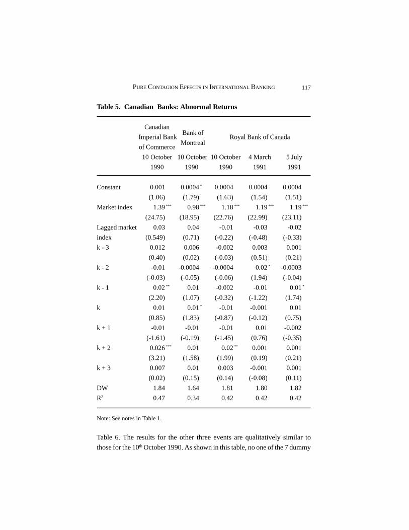
117PURE CONTAGION EFFECTS IN INTERNATIONAL BANKING
Table 5. Canadian Banks: Abnormal Returns
Canadian
Imperial Bank Royal Bank of Canada
of Commerce
10 October 10 October 10 October 4 March 5 July
1990 1990 1990 1991 1991
Constant 0.001 0.0004* 0.0004 0.0004 0.0004
(1.06) (1.79) (1.63) (1.54) (1.51)
Market index 1.39*** 0.98*** 1.18*** 1.19*** 1.19***
(24.75) (18.95) (22.76) (22.99) (23.11)
Lagged market 0.03 0.04 -0.01 -0.03 -0.02
index (0.549) (0.71) (-0.22) (-0.48) (-0.33)
k - 3 0.012 0.006 -0.002 0.003 0.001
(0.40) (0.02) (-0.03) (0.51) (0.21)
k - 2 -0.01 -0.0004 -0.0004 0.02* -0.0003
(-0.03) (-0.05) (-0.06) (1.94) (-0.04)
k - 1 0.02** 0.01 -0.002 -0.01 0.01*
(2.20) (1.07) (-0.32) (-1.22) (1.74)
k 0.01 0.01* -0.01 -0.001 0.01
(0.85) (1.83) (-0.87) (-0.12) (0.75)
k + 1 -0.01 -0.01 -0.01 0.01 -0.002
(-1.61) (-0.19) (-1.45) (0.76) (-0.35)
k + 2 0.026*** 0.01 0.02** 0.001 0.001
(3.21) (1.58) (1.99) (0.19) (0.21)
k + 3 0.007 0.01 0.003 -0.001 0.001
(0.02) (0.15) (0.14) (-0.08) (0.11)
DW 1.84 1.64 1.81 1.80 1.82
R2 0.47 0.34 0.42 0.42 0.42
Note: See notes in Table 1.
Table 6. The results for the other three events are qualitatively similar to
those for the 10th October 1990. As shown in this table, no one of the 7 dummy
Bank of
Montreal
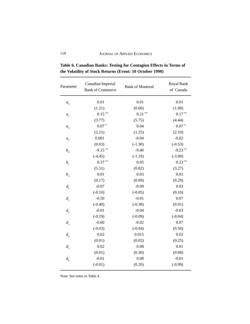
118 JOURNAL OF APPLIED ECONOMICS
Table 6. Canadian Banks: Testing for Contagion Effects in Terms ofthe Volatility of Stock Returns (Event: 10 October 1990)
Canadian Imperial Royal Bank
Bank of Commerce of Canada
a0
0.01 0.01 0.01
(1.21) (0.60) (1.08)
a1
0.15*** 0.21*** 0.17***
(3.77) (5.75) (4.44)
a2
0.07** 0.04 0.07**
(2.21) (1.25) (2.10)
a3
0.001 -0.04 -0.02
(0.03) (-1.30) (-0.53)
b0
-9.15*** -9.40 -9.23***
(-4.45) (-1.19) (-3.90)
b1
0.37*** 0.05 0.23***
(5.51) (0.82) (3.27)
b2
0.01 0.03 0.01
(0.17) (0.69) (0.29)
d0
-0.07 -0.09 0.03
(-0.10) (-0.05) (0.10)
d1
-0.50 -0.01 0.07
(-0.40) (-0.38) (0.01)
d2
-0.01 -0.04 -0.03
(-0.19) (-0.09) (-0.04)
d3
-0.60 -0.02 0.07
(-0.03) (-0.04) (0.50)
d4
0.02 0.015 0.02
(0.01) (0.02) (0.25)
d5
0.02 0.08 0.01
(0.01) (0.30) (0.08)
d6
-0.01 0.08 -0.01
(-0.01) (0.20) (-0.99)
Note: See notes in Table 4.
Parameter Bank of Montreal

119PURE CONTAGION EFFECTS IN INTERNATIONAL BANKING
variables is statistically significant, thereby suggesting that the event of the
10th October 1990 did not cause a volatility increase in the stock returns of
each of the three Canadian banks. A similar conclusion can be drawn for the
other three events. Therefore, there is no evidence of contagion effects for
the Canadian banks even in terms of volatility.
These results are in contrast to the findings of Jayanti et al. (1996), who
found some evidence of negative abnormal returns and negative cumulative
abnormal returns on the Canadian banking sector following the collapse of
two domestic banks, namely the Canadian Commercial Bank (CCB) and the
Northbank. This differing reaction may be accounted for by the fact that CCB
and Northbank were relatively larger banks in Canada than BCCI-Canada,
and by the large distance of BCCI’s headquarters from the headquarters of
the Canadian banks.18 According to Akhibe and Madura (2001), the smaller
the relative size of the assets of the failed bank in one country, the higher the
ability of ‘rival’ banks to withstand financial distress. In addition, the difference
of our results for Canada from those for the UK can be attributed to the
relatively higher size of the deposit insurance coverage in Canada, which is
up to US$ 52,000.19
Overall, the results for the US and Canada suggest that the failure of a
dishonestly run bank, even a large one, does not cause loss of confidence in
the integrity of the banking system as a whole. The standard regulatory
measures available, such as deposit insurance, appear to be sufficient in
protecting against contagion effects. In the UK, the existence of pure contagion
effects may be interpreted as an indication that UK capital markets were
concerned about the supervision of BCCI and the adequacy of the regulatory
system to prevent the collapse of the bank. This interpretation is in line with
the Bingham Report commissioned in the UK after BCCI’s failure. This report
raised several issues in relation to the supervision of BCCI in the UK, and
offered a number of detailed suggestions to strengthen it, including the need
for greater cooperation, greater sharing of information, strengthening of
18 CCB and Northbank were ranked 10th and 11th in Canada; BCCI-Canada was at a muchlower rank.
19 The Banker, 1 September 1991, ‘BCCI: How safe is your money?’, vol. 141, no 787.

120 JOURNAL OF APPLIED ECONOMICS
internal communications, and more efficient supervision of internationally
spread banking groups like BCCI.20
V. Conclusions
This study has examined the issue of contagion effects in international
banking arising from the failure of BCCI, one of the largest multinational
banks. As the failure of BCCI was due to fraud, this study offers an empirical
assessment of the ‘pure’ contagion effects hypothesis. We focused on the
three largest banks in three developed countries where BCCI had established
operations, namely the UK, the US, and Canada. Using event study
methodology, we tested for negative abnormal returns and negative cumulative
abnormal returns on individual banks surrounding several BCCI-related
announcements. Our analysis provides strong evidence of pure contagion
effects in the UK which have arisen prior to the official closure date, following
a BCCI-related announcement raising suspicions of irregularities and fraud
on a large scale in the bank’s operations. Our results suggest that stock prices
of all three UK banks reacted negatively to information about fraud in a large
bank’s activities. There is no evidence of pure contagion effects in the US
and Canada, even in terms of the volatility of bank stock returns, which
suggests that the regulatory measures available in these two countries appear
to be sufficient in preventing contagion effects arising from the failure of a
large bank with fraudulent activities. Our results for the UK are in line with
the Bingham Report, which offered several recommendations to strengthen
the supervision of internationally spread groups like BCCI.
20 Further recommendations included the establishment of a trained and qualified specialinvestigations unit to consider all warnings of malpractice, strengthening of the Bank ofEngland’s legal unit, and strengthening of the Bank’s powers to refuse authorisation on thegrounds that a bank cannot be effectively supervised. (Financial Times, 23 October 1992,‘Bingham report – Investigation into the BCCI scandal: The main recommendations’, page8). In response to this report, several measures were announced to strengthen the supervisionin the future. (Financial Times, 23 October 1992, ‘Bingham report – Investigation into theBCCI scandal: Governor outlines stronger measures’, page 8).

121PURE CONTAGION EFFECTS IN INTERNATIONAL BANKING
References
Aharony, Joseph, and Itzhak Swary (1983), “Contagion Effects of Bank
Failures: Evidence from Capital Markets,” Journal of Business 56: 305-322.
Aharony, Joseph, and Itzhak Swary (1996), “Additional Evidence on the
Information-based Contagion Effects of Bank Failures,” Journal of
Banking and Finance 20: 57-69.
Akhibe, Aigbe, and Jeff Madura (2001), “Why do Contagion Effects Vary
among Bank Failures?”, Journal of Banking and Finance 25: 657-680.
Benston, George (1973), “Bank Examination,” Bulletin of Institute of Finance,
May: 89-90.
Bollerslev, Tim, and Jeffrey M. Wooldridge (1992), “Quasi-maximum
Likelihood Estimation and Inference in Dynamic Models with Time-
varying Covariances,” Econometric Reviews 11: 143-155.
Bomfim, Antulio (2003), “Pre-announcement Effects, News Effects and
Volatility: Monetary Policy and the Stock Market,” Journal of Banking
and Finance 27: 133-151.
Calomiris, Charles, and Charles Kahn (1991), “The Role of Demandable Debt
in Structuring Optimal Banking Arrangements,” American Economic
Review 81: 497-513.
Chan, Yuk-Shee, Stuart Greenbaum, and Anjan Thakor (1992), “Is Fairly
Priced Deposit Insurance Possible?”, Journal of Finance 47: 227-246.
Diamond, Douglas, and Philip Dybvig (1983), “Deposit Insurance, Liquidity
and Bank Runs,” Journal of Political Economy 91: 401-419.
Dickinson, Amy, David Peterson, and William Christiansen (1991), “An
Empirical Investigation into the Failure of First Public Bank: Is there
Contagion?”, Financial Review 26: 303-318.
Dothan, Uri, and Joseph Williams (1980), “Banks, Bankruptcy and
Regulation,” Journal of Banking and Finance 4: 65-87.
Flannery, Mark (1995), “Prudential Regulation for Banks,” in K. Sawamoto,
Z. Nakajima and H. Taguchi, eds., Financial Stability in a Changing
Environment: 281-318, New York, St Martin’s Press.
Furfine, Craig H. (1999), “Interbank Exposures: Quantifying the Risk of
Contagion,” BIS Working Paper No 70: 1-26, Bank for International
Settlements, Monetary and Economic Department, Basel, Switzerland.

122 JOURNAL OF APPLIED ECONOMICS
Hall, Maximilian. (1991), “The BCCI Affair”, Banking World, September:
8-11.
Jacklin, Charles, and Sudipto Bhattacharya (1988), “Distinguishing Panics
and Information-based Bank Runs: Welfare and Policy Implications,”
Journal of Political Economy 96: 668-592.
Jayanti, Subbarao V., Ann Marie Whyte, and A. Quang Do (1996), “Bank
Failures and Contagion Effects: Evidence from Britain and Canada,”
Journal of Economics and Business 48: 103-116.
Lamy, Robert E., and G. Rodney Thompson (1986), “Penn Square, Problem
Loans, and Insolvency Risk,” Journal of Financial Research 9: 103-111.
Madura, Jeff, Alan Tucker, and Emilio Zarruk (1992), “Reaction of Bank
Share Prices to the Third-world Debt Reduction Plan,” Journal of Banking
and Finance 16: 853-868.
Masulis, Ronald W. (1980), “The Effects of Capital Structure Change on
Security Returns: A Study of Exchange Offers,” Journal of Financial
Economics 8: 139-177.
Murphy, Neil (1979), “Disclosure of the Problem Bank Lists: A Test of the
Impact,” Journal of Bank Research 10: 88-96.
Peavy, John III, and George Hempel (1988), “The Penn Square Bank Failure:
Effect on Commercial Bank Security Returns-A Note,” Journal of Banking
and Finance 12: 141-150.
Saunders, Anthony, and Michael Smirlock (1987), “Intra and Interindustry
Effects of Bank Securities Market Activities: The Case of Discount
Brokerage,” Journal of Financial and Quantitative Analysis 22: 467-482.
Slovin, Myron, and Subbarao V. Jayanti (1993), “Bank Capital Regulation
and the Valuation Effects of Latin American Debt Moratoriums,” Journal
of Banking and Finance 17: 159-174.
Smirlock, Michael, and Howard Kaufold (1987), “Bank Foreign Lending,
Mandatory Disclosure Rules, and the Reaction of Bank Stock Prices to
the Mexican Debt Crisis,” Journal of Business 60: 347-364.
Swary, Itzhak (1986), “Stock Market Reaction to Regulatory Action in the
Continental Illinois Crisis,” Journal of Business 59: 451-473.
The Banker (1991), “Unanswered Questions,” September: 12-19.
The Banker (1991), “Top 1000 Banks by Country,” July: 15-25.
Zellner, Arnold (1962), “An Efficient Method of Estimating Seemingly

123PURE CONTAGION EFFECTS IN INTERNATIONAL BANKING
Unrelated Regression and Tests of Aggregate Bias,” Journal of American
Statistical Association 57: 348-368.

125GOVERNMENT EXPENDITURE AND ECONOMIC GROWTH
Journal of Applied Economics, Vol. VIII, No. 1 (May 2005), 125-152
GOVERNMENT EXPENDITURE ANDECONOMIC GROWTH: EVIDENCE FROM
TRIVARIATE CAUSALITY TESTING
JOHN LOIZIDES * AND GEORGE VAMVOUKAS
Athens University of Economics and Business
Submitted February 2001; accepted May 2004
This paper seeks to examine if the relative size of government (measured as the share oftotal expenditure in GNP can be determined to Granger cause the rate of economic growth,or if the rate of economic growth can be determined to Granger cause the relative size ofgovernment. For this purpose, we first use a bivariate error correction model within aGranger causality framework, as well as adding unemployment and inflation (separately)as explanatory variables, creating a simple ‘trivariate’ analysis for each of these two variables.The combined analysis of bivariate and trivariate tests offers a rich menu of possible causalpatterns. Using data on Greece, UK and Ireland, the analysis shows: i) government sizeGranger causes economic growth in all countries of the sample in the short run and in thelong run for Ireland and the UK; ii) economic growth Granger causes increases in therelative size of government in Greece, and, when inflation is included, in the UK.
JEL classification codes: H21
Key words: public sector growth, economic growth, bivariate and trivariate
causality tests, error correction modeling
I. Introduction
The size of government expenditures and its effect on long-run economic
growth, and vice versa, has been an issue of sustained interest for decades.
* Loizides (corresponding author): Athens University of Economics & Business, 76 PatissionSt., Athens 104 34, Greece; e-mail: [email protected]. Vamvoukas, e-mail:[email protected]. The authors wish to thank the editor and the anonymous refereesof this Journal for their helpful comments. All remaining errors and deficiencies are theresponsibility of the authors.

126 JOURNAL OF APPLIED ECONOMICS
The received literature, essentially of an empirical nature, has proceeded at
two levels.
One set of studies has explored the principal causes of growth in the public
sector. Wagner’s Law -the “Law of increasing expansion of public and
particularly state activities” (Wagner, 1893)- is one of the earliest attempts
that emphasises economic growth as the fundamental determinant of public
sector growth. Empirical tests of this hypothesis, either in the form of standard
regression analysis (see, for instance, Ganti and Kolluri, 1979; and
Georgakopoulos and Loizides, 1994, to cite only a few) or in the form of
error-correction regression (see, for instance, Kolluri, Panik and Wanab, 2000,
and the literature cited therein), have yielded results that differ considerably
from country to country.
The other set of studies has been directed towards assessing the effects of
the general flow of government services on private decision making and,
more specifically, on the impact of government spending on long-run economic
growth. Macroeconomics, especially the Keynesian school of thought, suggests
that government spending accelerates economic growth. Thus, government
expenditure is regarded as an exogenous force that changes aggregate output.
Here, again, empirical work, either in standard regression forms (see, for
instance, Landau, 1983) or error-correction regressions (see, for instance,
Ghali, 1998, and the literature cited therein) finds diverse results.
Although each line of enquiry has thrown interesting light on the
phenomena, in neither case has the assumed causative process been subjected
to rigorous empirical pre-testing. Purely a priori judgements for choosing
between the two competing postulates are rendered difficult for at least three
reasons: Firstly, there is the possibility of feedback in macro relations, which
tend to obscure both the direction and the nature of causality. Secondly, as
demonstrated by Ahsan, Kwan and Sahni (1992), in the public expenditure-
national income nexus, failure to account for omitted variables can give rise
to misleading causal ordering among variables and, in general, yields biased
results. Thirdly, if co-integration among the variables of the system is admitted,
then the error-correction terms would provide an additional source of causality.
Indeed, a principal feature of cointegrated variables is that their time paths
are influenced by the extent of any deviation from long-run equilibrium. Thus,
omission of the error correction terms would entail a mispecification error

127GOVERNMENT EXPENDITURE AND ECONOMIC GROWTH
and potentially bias the results. In the context of trivariate systems such an
outcome is very possible because the introduction of a third variable in the
system can alter the causal inference based on the simple bivariate system.
Singh and Sahni (1984) initially examined the causal link between
government expenditure and national income. Subsequently, their work has
generated many other studies, the results of which range the full continuum
from no causality to bi-directional causality between these two variables. Ram
(1986, 1987), among the existing causality studies, suggested that differences
in the nature of underlying data, the test procedure and the period studied
may explain the diversity in results. A few years later, Ahsan, Kwan and
Sahni (1992) added various other factors that may explain the inconsistency
amongst the results obtained by different authors, one of which is the influence
of ‘omitted’ variables. It is suggested that failure to account for omitted
variables can give rise to a misleading causal ordering among the variables.
To the best of our knowledge, this study is the only one that examines the
causal link between public sector size and GNP within a trivariate framework.
Recently, various other studies have used the cointegration test results, but in
the context of a bivariate approach, to either validate or invalidate Wagner’s
Law (see, for instance, Hondroyiannis and Papapetrou,1995; Bohl, 1996;
Chletsos and Kollias, 1997; Kolluri et al., 2000, and the literature cited therein).
The only study that follows a methodology similar to ours is Ghali (1998).
That study uses multivariate cointegration techniques but puts the emphasis
on a different place.
A significant weakness of many of the previous studies on this topic (save
for Ghali’s, 1998 study) was the failure to adjust for the co-integration result
of the time series in the case of the trivatiate framework, that renders traditional
statistical inference invalid. Indeed, as we will discuss below, the introduction
of a third variable in the system can alter not only the causal inference based
on the simple bivariate system, but also the magnitude of the estimates.
The principal aim of this paper is to empirically evaluate the causal link
between the size of the public sector and real per capita income within the
bivariate and trivariate frameworks, by resorting to recent developments in
the theory of cointegrated processes. The combined analysis of bivariate and
trivariate tests offers a rich menu of possible causal patterns. To this end, we
employ cointegration analysis, error-correction modelling and multivariate

128 JOURNAL OF APPLIED ECONOMICS
causality tests. We conducted three different specifications: i) in the first, we
test for a causal link between the size of the public sector, as measured by the
ratio of government expenditure relative to GNP (hereafter denoted as Gt),
and real per capita income (hereafter denoted as Yt) at the bivariate level; ii)
in the second we include Gt, Y
t and the unemployment rates; and iii) in the
third we substitute the unemployment rates by the inflation rates. The last
two specifications are intended to investigate whether, by switching to a
trivariate system from the bivariate one, the causality results would leave
unchanged the causal link between Gt and Y
t in every case examined. Should
Granger causality of a certain pattern be robust to the specification changes
from bivariate to trivariate system, one would have more confidence in the
predictive power of the underlying causal process. Besides, since trivariate
tests incorporate more information than bivariate ones, the causal inferences
drawn appear more reliable.
A question that naturally arises is how do we determine which variable
has to be included in the specification of the system. This is difficult to answer,
given that the studies in these areas are empirical in orientation. In principle,
any variable that is intimately connected with the size of public sector as well
as national income could be used. In this paper, we decided to use
unemployment and inflation rates for two reasons. First, during the period
examined these variables were at the centre of interest of economic policies.
Indeed, compared with the relatively placid and successful decades of the
1950s and 1960s in most European countries, the 1970s and afterwards was
accompanied not only by rising unemployment on a scale not previously
experienced since the inter-war years, but also by very strong inflationary
pressures. We therefore expect inflation and unemployment to play an
important role in the formation of the causal process between G and Y.
Secondly, various empirical studies find that both unemployment and inflation
are intimately connected with the size of public sector growth and national
income. For example, Abrams (1999) presents evidence that the rise in US
government outlays (as a percent of GDP since 1949) is responsible for
increases in the unemployment rate, which have contributed to slow down
the growth of the US economy. On the other hand, a number of authors, such
as Fischer (1993), Burdekin, Goodwin, Salamun and Willet (1994), and Clark

129GOVERNMENT EXPENDITURE AND ECONOMIC GROWTH
(1997), estimate time-series regressions of growth and inflation across
countries and find inflation to be inversely related to growth.
We applied trivariate causality tests using time series data drawn from
three European countries over the period from early 1950s to mid-1990s.
One developed country, the United Kingdom, and two developing countries;
namely, Ireland and Greece were selected for investigation. Since empirical
work on this topic covers both developed and developing nations, it is of
interest to test whether similar or different results hold between these two
categories of countries.
The rest of the paper proceeds as follows. In section II we briefly outline
the data set and provide some stylised facts of the main characteristics of the
variables that we used in the analysis. Section III considers some theoretical
issues as well as some empirical results of past studies. In section IV we
present the econometric methodology. Section V provides the empirical results
of our study, while section VI concludes.
II. Data and some Stylized Facts
The data set used in this study relates to the UK, Greece and Ireland and
consists of annual observations. Income, Yt, is measured as real per capita
Gross National Product (GNP) at market prices in year t. Real government
expenditure is measured as the Public Authorities spending on goods and
services (excluding transfer payments), i.e. consumption and gross fixed capital
formation. Public sector size Gt, is measured as the ratio of real government
expenditure to GNP. Unemployment rate UNt, is calculated as the unemployed
persons divided by the working population. Pt, is the wholesale price index
and its change, Dln Pt, gives the inflation rate .tP& For the UK and Ireland, data
for Yt, G
t, and P
t, come from the IMF’s International Financial Statistics,
while data for UNt, are taken from the European Economy published by the
European Commission. The statistical data for Greece come from the National
Accounts and the Labour Force Organization and cover the time period 1948-
1995. For the UK and Ireland, the annual time series runs from 1950 through
1995. Note, however, that in UK and Ireland, data for the UNt series cover the
period 1960 to 1995, since data are not available before 1960. All variables

130 JOURNAL OF APPLIED ECONOMICS
are expressed in natural logarithms; hence their first differences approximate
the growth rates.
In the choice of government size we follow the procedure adopted by
practically all scholars to date and relate government spending to GNP.
Practices, however, are more varied as to which types of public expenditures
one should relate to GNP and whether one should use deflated or undeflated
data. Researchers have also used differing approaches regarding the inclusion
of transfer payments in the size of the public sector. For example, Ram (1986)
argued that transfer payments should be excluded to make government
spending compatible with Wagner’s ideas. Musgrave and Musgrave (1980)
also excluded transfer payments from government expenditure for the reason
that their inclusion overstates the size of government. Recent works by Ahsan,
Kwan and Sahni (1996) and Ghali (1998), utilise an aggregate measure of Gt
inclusive of transfer payments in their analysis. However, since the intention
of this paper is to investigate the causal chain between the size of public
sector and economic growth, transfer payments were excluded, in order to be
able to differentiate the effects of income redistribution and provision of public
services on growth.
Opinions differ concerning the choice of whether one should use deflated
or undeflated measures of government size.1 As it is possible to find viable
arguments both in favour and against the use of deflated ratios, we have decided
to use deflated measures of government size in this paper.
Before proceeding to the estimation of the causal link between Gt and Y
t,
it is of interest to have a bird’s eye view of the basic characteristics of the
variables used in this study.2 The evolution of Gt, Y
t and growth rates of GNP,
together with unemployment and inflation rates, during the period 1960-1995
reveals some interesting findings. First, government spending in Greece during
the 1960s was around 19.0 per cent of GNP, some 3 percentage points lower
than in the UK and 1 percentage point lower than in Ireland. During the 25
years since then, the rise in spending in Greece has been more than in Ireland
and in the UK, with the result that now spending is highest there. It was only
after the Maastricht Treaty (1992) that public spending control in Greece
1 See, for instance, Cullis and Jones (1987).
2 To conserve space, this set of data is omitted but it is available upon request.

131GOVERNMENT EXPENDITURE AND ECONOMIC GROWTH
became an important objective of economic policy with the aim of gaining
admission to the European Monetary Union.
Second, in terms of the level of economic development, the UK is by far
the more developed country. Throughout most of the period, and especially
during the 1960s, real per capita income in the UK was nearly twice the
levels of Ireland and Greece. However, these differences have changed
substantially over time. On average, real per capita incomes in Greece and
Ireland rose around 1 per cent a year during the period, whereas in the UK
there was an absolute contraction at the rate of 0.5 per cent per annum. Real
per capita incomes in Greece, which had been previously rising, were reversed
after the early 1980s, and between 1986 and 1990 fell on average by about 12
per cent. On the contrary, in Ireland real per capita income increased by 6 per
cent during the same period. By the mid 1990s, real per capita income levels
in Ireland were about 30 per cent higher than those in Greece, and only 10 per
cent lower than those of the UK.
Third, relating growth rates of public spending to the growth rates of GNP
among these countries, two general remarks are in order. First, growth rates
of GNP declined everywhere from the rates prevailing in the 1960s, but in
Greece this reduction was much greater. Second, and less obvious, during the
period growth rates of government expenditures in the UK and Ireland declined
in much the same way as the growth rates of GNP, whereas in Greece
government spending grew at a faster rate than GNP (some 3 percentage
points). Even in this very rudimentary way, we observe a long-run constraining
relationship between the growth of GNP and the growth of expenditure in the
UK and Ireland. Thus, the fact to be explained in these two countries is not
the high variability of government expenditure but rather its remarkable
stability with respect to the trend growth of national income.
Finally, for much of the 1970s and early 1980s inflation was one of the
overriding issues in all three countries, often running into double figures. All
three economies displayed significant deterioration in inflation performance
after 1974. However, whereas Irish and British inflation fell significantly after
1985, inflation in Greece persisted. Nevertheless, one problem that refused
to go away was unemployment. In fact, until the middle of the 1990s
unemployment was on an upward trend, rising into double figures in Ireland
and close to 10 percent in the UK and Greece.

132 JOURNAL OF APPLIED ECONOMICS
III. Theoretical Issues and Empirical Evidence
The substantial growth of the size of government expenditures in both the
developed and developing nations since World War II, and its effect(s) on
long-run economic growth (or vice versa), has spawned a vast literature that
offers diverse attempts to explain the observed phenomenon.
On the one hand, public finance studies have been directed towards
identifying the principal causes of public sector growth.3 Wagner’s Law of
public expenditure is one of the earliest attempts that emphasize economic
growth as the fundamental determinant of public sector growth. The literature
on this topic is immense to say the least. Some studies find a significant
positive relationship between public sector growth and economic growth only
for developing nations but not for developed countries. Others even report a
negative relationship between government spending and GNP.
On the other hand, macroeconomics, especially the Keynesian school of
thought puts the emphasis on a different place. The analysis bears upon the
question of the role of government in economic growth. A considerable amount
of attention has been directed towards assessing the effect of the general flow
of government services on economic growth.4
During the last twenty years or so, studying the underlying causal process
3 Henrekson and Lybeck (1988) provide an excellent survey of various hypothesesconcerning the sources of growth of government expenditures.
4 Several studies have examined the relationship between the growth rate of real per capitaoutput and the share of government spending and find diverse results. For example, Landau(1983), in a cross-section study of over 100 countries in the period 1961-76, reportedevidence of a negative relationship between the growth rate of real per capita GDP and theshare of government consumption expenditure in GDP. By contrast, Ram (1986), utilisinga two-sector model, in a cross-section study of 115 countries and in the two-decade periodfrom 1960 through 1980, found that growth of government size has a positive effect oneconomic growth. Barro (1991) reports mixed results. In his cross-section study of 98nations between the years 1960 and 1985, he found that increases in government consumptionexpenditure measured as a percent of national income reduce per capita growth. However,when the share of public investment was considered, Barro found a positive but statisticallyinsignificant relationship between public investment and the output growth rate. Finally, inthe United States, Razzolini and Shughart (1997) present evidence that growth in the relativesize of government is responsible for a decrease in the US growth rate.

133GOVERNMENT EXPENDITURE AND ECONOMIC GROWTH
between government spending and GDP, or their close variants, has made
parallel efforts. The principle reason that led researchers to this field of analysis
was the difficulty of a possible feedback in macro relations, which tend to
obscure both the direction and the nature of causality.
It is clear that knowledge of the true nature of the causative process between
government spending and GDP will help determine the robustness of the
estimated relationship. Should the causality be Wagnerian, the estimates
derived from macro-econometric models would evidently suffer from
simultaneity bias. On the other hand, if the causality were Keynesian, the
estimates reported in public finance studies would similarly be biased.
Nevertheless, knowledge of the precise causative process has important policy
implications. For example, if the causality were Wagnerian, public expenditure
is relegated to a passive role, if Keynesian, it acquires the status of an important
policy variable.
Singh and Sahni (1984), using the Granger-Sims methodology, initially
examined the causal link between government expenditure and national
income in a bivariate framework. Their empirical results, based on data for
India, suggest that the causal process between public expenditure and national
income is neither Wagnerian nor Keynesian. Similarly, Ahsan, Kwan, and
Sahni (1992) have used the same approach, but in a trivariate framework.
Their interesting results indicate that while the US data fail to detect any
causality between public expenditure and national income at the bivariate
level, there was strong evidence of indirect causality from GDP to public
spending via both money stock and budgetary deficits. Bohl (1996) applied
tests of integration, cointegration and Granger causality in a bivaritate context,
and found support to Wagner’s law for only the United Kingdom and Canada,
out of the G7 countries,5 during the post-World War II period. Hondroyiannis
and Papapetrou (1995), and Chletsos and Kollias (1997), applied the same
methodology in Greece, and found mixed results. To our knowledge, Ghali’s
(1998) study is the only one that uses multivariate cointegration techniques,
and examines the dynamic interactions between government size and economic
growth in a five-variable system, consisting of the growth rates of GDP, total
5 These countries are Canada, France, Germany, Italy, Japan, the United Kingdom and theUnited States.

134 JOURNAL OF APPLIED ECONOMICS
government spending, investment, exports, and imports. Using data from ten
OECD countries, Ghali’s study shows that government size Granger-causes
growth in all countries of the sample. More recently, Kolluri, et. al. (2000),
using a bivariate framework, estimated the long-run relationship between gross
domestic product and government spending in the G7 countries for the period
1960-1993. Most of their empirical findings confirm Wagner’s Law for the
G7 countries; that is, government spending tends to be income elastic in the
long run. This disparate evidence calls for a re-examination of the differences
in the causality results.
As we mentioned in the introduction, the focus of this paper is to
empirically evaluate the causal link between Gt and Y
t within the bivariate
and trivariate frameworks, by resorting to recent developments in the theory
of cointegrated process. Models that use only levels of variables or first
differences (see for instance Singh and Sahni, 1984, and Ahsan et al., 1992),
are mispecified because they ignore interim short-run corrections to long-run
equilibrium. Besides, in the case of the trivariate approach this problem, as
we will show below, is even stronger because the third variable can alter the
causal inference based on the simple bivariate system.
IV. Econometric Methodology
The notion that there is a long-run tendency for the public sector to grow
relative to national income or vice-versa has been an issue in economics that
is rarely questioned. Thus, if the variables Yt and G
t are considered as stochastic
trends and if they follow a common long-run equilibrium relationship, then
these variables should be cointegrated. According to Engle and Granger
(1987), cointegrated variables must have an ECM representation. The main
reason for the popularity of cointegration analysis is that it provides a formal
background for testing and estimating short-run and long run relationships
among economic variables. Furthermore, the ECM strategy provides an answer
to the problem of spurious correlation.6
If Yt and G
t are cointegrated, an ECM representation could have the
following form:
6 For a useful discussion of spurious correlations and ECM strategy, see Enders (1998).

135GOVERNMENT EXPENDITURE AND ECONOMIC GROWTH
0 1 1 2 31 1
[1 ] [1 ]n n
t t i t i i t i ti i
Y a a E a L Y a L G u∆ ∆ ∆− − −= =
= + + − + − +∑ ∑
where L and D are the lag and difference operators, respectively, and Et-1
, Ct-1
are error-correction terms. The error correction term Et-1
in (1) is the lagged
value of the residuals from the OLS regression of Yt on G
t and the term C
t-1 in
(2) corresponds to the lagged value of the residuals from the OLS regression
of Gt on Y
t. In (1) and (2), DY
t, DG
t, u
t and e
t are stationary, implying that their
right-hand side must also be stationary. It is obvious that (1) and (2) compose
a bi-variate VAR in first differences augmented by the error-correction terms
Et-1
and Ct-1
, indicating that ECM model and cointegration are equivalent
representations.
According to Granger (1969; 1988), in a cointegrated system of two series
expressed by ECM representation causality must run in at least one way. Within
the ECM formulation of (1) and (2), Gt does not Granger cause Y
t if all a
3i = 0
and a1 = 0. Equivalently, Y
t does not Granger cause G
t if all b
2i = 0 and b
1 = 0.
However, it is possible that the causal link between Yt and G
t estimated from
the ECM formulation (1) and (2) could have been caused by a third variable.
Such a possibility may be explored within a multivariate framework including
other important variables, such as the unemployment rates UNt or inflation rates
,tP& which represent considerable determinants of real GNP and government
expenditures. Thus, the causal relationship between Yt and G
t can be examined
within the following ECM representation:
where Zt could be the macroeconomic state of the economy. Regarding
(1)
0 1 1 2 31 1
[1 ] [1 ]n n
t t i t i i t i ti i
G b b C b L Y b L G e∆ ∆ ∆− − −= =
= + + − + − +∑ ∑ (2)
0 1 1 2 31 1
[1 ] [1 ]n n
t t i t i i t ii i
Y E L Y L Gα α α α∆ ∆ ∆− − −= =
= + + − + −∑ ∑
41
[1 ]n
i t i ti
L Z uα ∆ −=
+ − +∑
(3)
0 1 1 2 31 1
[1 ] [1 ]n n
t t i t i i t ii i
G C L Y L Gβ β β β∆ ∆ ∆− − −= =
= + + − + −∑ ∑
41
[1 ] ,n
i t i ti
L Z eβ ∆ −=
+ − +∑
(4)

136 JOURNAL OF APPLIED ECONOMICS
unemployment rates UNt, or inflation rates, tP& as ‘third’ variables, the system
captures the response of Yt and G
t to changes in UN
t, or .tP& The difference
between the ECM models (1) and (2), and (3) and (4) is that the introduction
of UNt, and tP& could alter the causal inference based on the simple bivariate
system. This occurs in one of three ways. First, the coefficients a2i
and a3i (b
2i
and b3i) need not be similar to a
2i and a
3i (b
2i and
b
3i), respectively, either in
direction or in magnitude. Second, Yt and G
t can be related through UN
t or
tP& even though the parameters a3i
and b2i are statistically insignificant. In
other words, any spurious causality that arises in the bivariate system may be
removed due to the presence of UNt or .tP& Finally, we may also find direct
causality between Gt and Y
t in a trivariate context, which may or may not be
detected, in a bivariate framework. In this latter scenario, the third variable
itself explains the causation. Thus, causality tests reported in earlier studies
(see, for instance, Hondroyiannis and Papapetrou,1995; Bohl, 1996; Chletsos
and Kollias, 1997; and Kolluri et al., 2000) might simply be artefacts of
mispecified models.
V. Empirical Results
To test formally for the presence of a unit root for each variable in the
model, Augmented Dickey-Fuller (ADF) and Phillips-Perron (PP) tests of
the type given by regression (5) and (6) were conducted. The ADF test is
conducted using the regression of the form:
where DWt are the first differences of the series W, k is the lag order and t
stands for time. Equation (5) is with constant and time trend.
PP tests involve computing the following OLS regression:
where a0, a
1, a
2 are the conventional least-squares regression coefficients. The
hypotheses of unit-root to be tested are H0 : a
1 = 1 and H
0 : a
1 = 1, a
2 = 0.
0 1 11
,k
t t i t i ti
W a a t W W u− −=
= + + + +∑ρ λ∆ ∆ (5)
0 1 1 2( / 2) ,t t tW a a W a t T u−= + + − + (6)
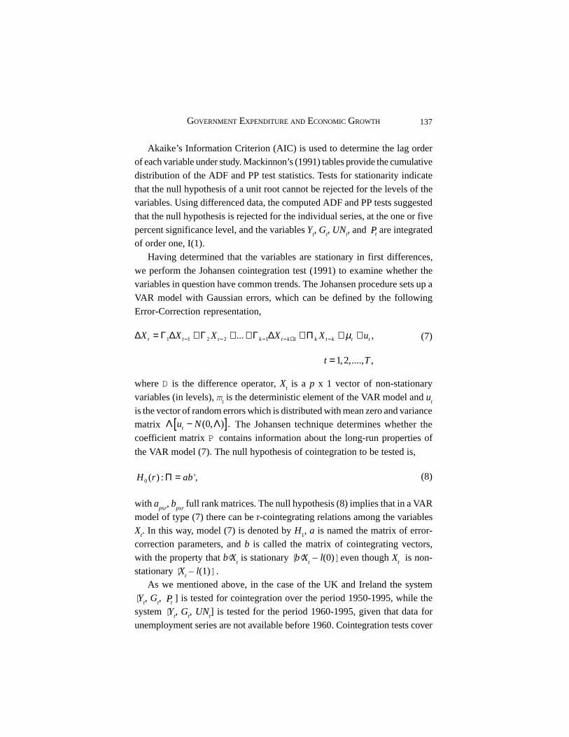
137GOVERNMENT EXPENDITURE AND ECONOMIC GROWTH
Akaike’s Information Criterion (AIC) is used to determine the lag orderof each variable under study. Mackinnon’s (1991) tables provide the cumulativedistribution of the ADF and PP test statistics. Tests for stationarity indicatethat the null hypothesis of a unit root cannot be rejected for the levels of thevariables. Using differenced data, the computed ADF and PP tests suggestedthat the null hypothesis is rejected for the individual series, at the one or fivepercent significance level, and the variables Y
t, G
t, UN
t, and tP& are integrated
of order one, I(1).Having determined that the variables are stationary in first differences,
we perform the Johansen cointegration test (1991) to examine whether thevariables in question have common trends. The Johansen procedure sets up aVAR model with Gaussian errors, which can be defined by the followingError-Correction representation,
where D is the difference operator, Xt is a p x 1 vector of non-stationary
variables (in levels), mt is the deterministic element of the VAR model and u
t
is the vector of random errors which is distributed with mean zero and variancematrix [ ](0, ) .tu NΛ − Λ The Johansen technique determines whether thecoefficient matrix P contains information about the long-run properties of
the VAR model (7). The null hypothesis of cointegration to be tested is,
with apxr
, bpxr
full rank matrices. The null hypothesis (8) implies that in a VARmodel of type (7) there can be r-cointegrating relations among the variablesX
t. In this way, model (7) is denoted by H
1, a is named the matrix of error-
correction parameters, and b is called the matrix of cointegrating vectors,with the property that b¢X
t is stationary [b¢X
t – l(0)] even though X
t is non-
stationary [Xt – l(1)] .
As we mentioned above, in the case of the UK and Ireland the system[Y
t, G
t,
tP& ] is tested for cointegration over the period 1950-1995, while thesystem [Y
t, G
t, UN
t] is tested for the period 1960-1995, given that data for
unemployment series are not available before 1960. Cointegration tests cover
1 1 2 2 1 1... ,t t t k t k k t k t tX X X X X uµ∆ Γ ∆ Γ Γ ∆ Π− − − − + −= + + + + + +
1,2,...., ,t T=
(7)
0( ) : ',H r abΠ == (8)

138 JOURNAL OF APPLIED ECONOMICS
the period 1948-1995 for Greece. In determining the number of cointegrating
vectors r, we use the maximum eigenvalue statistics, lmax
. The null hypothesis
to be tested is that there can be r cointegrating vectors among the three-
variable systems [Yt, G
t, UN
t] and [Y
t, G
t,
tP& ]. In order to check the robustness
of the results to the order of the VAR, we carry out the Johansen cointegration
tests using one and two year lag lengths. As to the cointegration test results,
the lmax
rank tests indicate that each group of the series is cointegrated. The
LR-tests are statistically significant, at the one and five percent levels, thus
rejecting the null hypothesis of noncointegration.7
Having verified that each group of the series Yt, G
t, and ,tP& Y
t, G
t and UN
t,
is cointegrated, we next investigate the causal pattern between Yt and G
t,
within the ECM models. In Table 1 we employ Hendry’s general-to-specific
strategy to estimate the bivariate ECM model (1) and (2), whereas Tables 2
and 3 present the same methodology in the case of trivariate ECM models of
the form (3) and (4). Five lags are used for each independent variable. The
lag length is reduced to five years to conserve degrees of freedom. The error-
correction terms Et-1
and Ct-1
serve as measures of disequilibrium, representing
stochastic shocks in the dependent variables, Yt and G
t, respectively. They
represent the proportion by which the long-run disequilibrium in the dependent
variables is corrected in each short-term period. The coefficients on Et-1
and
Ct-1
are expected to be negative and statistically significant. The coefficients
on the lagged values of DYt, DG
t, DUN
t and Dln P
t are short-run parameters
measuring the immediate impact of independent variables on DYt and DG
t.
The rationale of Hendry’s general-to-specific approach is to re-estimate the
basic model by dropping the lagged variables with insignificant parameters
from the system. In the restricted model we include lagged values of
independent variables significant at the 10 percent level. The restricted
equations are nested within the unrestricted models.8 In this sense, when
equations are special cases of a general model, they appear to be nested within
the general model.
The various specification and diagnostic tests applied in the restricted
7 Detailed regression results are available from the authors and will be supplied on request.
8 In order to conserve space, we present only the results of the restricted models. Unrestrictedmodels are available upon request.

139GOVERNMENT EXPENDITURE AND ECONOMIC GROWTH
equations DYt and DG
t appear significant and robust, indicating that the
estimated ECM models fit the data adequately. Choosing 1975 as the sample
breaking values of the parameter yield a stable solution, which is not sensitive
to changes in the sample range.9 The RESET (Regression Specification Test)
statistics reveal no serious omission of variables, indicating the correct
specification of the model. The ARCH (AutoRegressive Conditional
Heteroskedasticity tests suggest that the errors are homoskedastic and
independent of the regressors. The BG (Breusch-Godfrey) tests reveal no
significant serial correlation in the disturbances of the error term. The JB
(Jarque-Bera) statistics suggest that the disturbances of the regressors are
normally distributed. In sum, specification and diagnostic testing ensure that
the general model is congruent and that the congruency is maintained through
the restricted equations.
Table 1 presents the ECM results within the bivariate system for Greece,
UK and Ireland.10 Several conclusions are apparent. The essential result in
Greece is that economic growth Granger causes public spending expansion
but not the other way round. Thus, there is a high degree of support for this
Wagner type phenomenon in the data for Greece; public spending tends to be
income elastic in the long run.11 Note, however, that real per capita income
growth never enters significant in the restricted equation. This fact is an
indication that expenditure plans are too “sticky” to change in the light of
short-term fluctuations in income. Nevertheless, the Keynesian view about
the causal effects of public expenditures on economic growth has become
apparent in the short run.
9 Note that in all three countries, varying the sample breaking date, the Chow F-statisticsshow the stability of the ECM models over the chosen sub-periods.
10 To avoid overburdening the analysis with symbols, in this part, the time subscript isomitted from all variables.
11 Hondroyiannis and Papapetrou (1995) cast doubt on the validity of Wagner’s hypothesisin Greece, whereas Chletsos and Kollias (1997) found mixed results. Note, however, thatthe findings of these studies are not directly related to our results, merely because theydefined government size as the ratio of total spending (including transfer payments) toGNP. Even in that case, their results may be artefacts of mispecified models. This mayhappen because they use standard Granger causality tests, in a bivariate context, withoutallowing for the influence of the error correction terms.

14
0JO
UR
NA
L OF A
PP
LIED E
CO
NO
MIC
S
Table 1. Bivariate Estimates of Restricted ECMs
Greece United Kingdom Ireland
DYt
DGt
DYt
DGt
DYt
DGt
Constant 0.01 (1.31) --- --- --- 0.00 (0.01) -0.00 (-0.42)
DYt (-1) 0.33 (2.35)* --- 0.40 (2.56) --- 0.25 (1.58) ---
DYt (-2) --- --- 0.38 (2.59)* --- --- ---
DYt (-3) 0.34 (2.41)* --- --- --- 0.30 (2.01)* ---
DYt (-5) --- --- --- --- 0.30 (2.08)* ---
DGt (-1) 0.16 (2.28)* -0.14 (-1.04) -0.15 (-1.18) 0.94 (4.207)* --- 0.72 (4.70)*
DGt (-2) --- --- 0.26 (2.68)* -0.61 (-4.135)* --- -0.56 (-3.39)*
DGt (-4) --- --- --- --- 0.23 (3.09)* ---
Et-1
-0.02 (-1.16) --- -0.46 (-3.39)* --- -0.99 (-5.18)* ---
Ct-1
--- -0.30 (-3.17)* --- -0.47 (-1.69) --- 0.01 (1.24)
2R 0.30 0.21 0.23 0.41 0.54 0.40
DW 2.05 --- --- --- 1.86 2.04
SER 0.03 0.06 0.02 0.01 1.95 0.04
Chow (1975) 1.43 0.26 1.09 0.25 0.76 1.31
JB 0.02 2.62 1.61 0.48 0.08 0.77
Variables

141G
OV
ER
NM
EN
T EX
PE
ND
ITU
RE A
ND E
CO
NO
MIC G
RO
WT
H
RESET (1) 0.00 0.14 1.61 1.93 0.91 0.24
ARCH (2) 0.20 0.01 2.50 0.79 1.20 0.14
ARCH (3) 0.28 0.01 2.02 0.75 0.79 0.15
BG(2) 0.09 0.40 0.35 0.78 0.74 0.05
BG(3) 0.07 0.26 0.27 0.54 0.50 0.27
Notes: * is significant at the 5% level. Asymptotic t-statistics in parentheses. The error-correction term Et-1
(lagged one period) is the residual seriesfrom the regression of Y
t on G
t. Likewise, C
t-1 (lagged one period) is the residual from the corresponding regression of G
t on Y
t. 2R is the adjusted
R2. DW is the Durbin-Watson statistic. SER is the standard error of the regression. Chow is the F-statistic for structural change in 1975. JB is theJarque-Bera test for the normality of the regression residuals. RESET is the Ramsey F-statistic for omitted variables. BG is the Breusch-GodfreyF-statistic. ARCH is the Autoregressive Conditional Heteroskedasticity F-statistic. In RESET, BG and ARCH tests, numbers in parentheses are thelag lengths.
Table 1. (Continued) Bivariate Estimates of Restricted ECMs
Greece United Kingdom Ireland
DYt
DGt
DYt
DGt
DYt
DGt

142 JOURNAL OF APPLIED ECONOMICS
By contrast, for Ireland and the UK, our estimates show one-way causality
running from G to Y. These results are consistent with the Keynesian notion
suggesting that the causal linkage flows from DG to DY both in the long run
and the short-run. The fact that public spending in these two countries is
income inelastic in the long run simply indicates some long-run proportionality
between the size of public sector growth and GNP. This of course was only to
be expected given that, as we mentioned in section II, in these countries
government size kept pace with national income and, indeed, during the 1980s
income has grown just a little faster than public sector size. The behaviour of
the institutions that determine public expenditure, perhaps, explains its stability.
Indeed, at least in the UK, the institutional procedures adopted for
expenditure planning deliberately target expenditure growth on the expected
growth of national income. For instance, following the 1961 Plowden Report,
expenditure planning in Britain was institutionalised in the Public Expenditure
Survey Committee system. The intention of this system was to plan public
expenditure over a five-year horizon in relation to prospective resources. Real
public expenditure was projected as a stable share of the anticipated future
level of real income. On the contrary, the whole process of budgeting in Greece
-one year non-zero budgeting- has incentives to facilitate and maintain
bureaucratic growth and to supply a level of expenditures higher than that
which would result from simple majority rule.
Note that the sign of coefficient estimate Ct-1
, in the regression DG for
Greece, is negative and statistically significant, which supports convergence
of the size of public sector growth to its conditional mean, determined by
GNP growth. That is, the sign is in accord with convergence toward the long-
run equilibrium and the results support Wagner’s Law for Greece. It indicates
that about one third (30 percent) of any disequilibrium between actual and
equilibrium public sector size, in any period, is made up during the current
period. Thus, the size of public sector growth in Greece responds mainly to
the trend level of real per capita income, rather than to its short-term variations.
This sort of sluggish adjustment process is, as we noted above, an indication
that expenditure plans are too rigid to change in line with short-term
fluctuations in income.
Similarly, the coefficients Et-1
in the regression DY for the UK and Ireland
are statistically significant and they support convergence of real per capita

143GOVERNMENT EXPENDITURE AND ECONOMIC GROWTH
income growth to its conditional mean determined, in part, by government
spending growth. It is hardly surprising, however, that in the UK the long run
growth effect of public sector size on economic growth is quite sluggish as
compared to that of Ireland. Indeed, in the UK, the response of real per capita
income growth to its previous period disequilibrium is only half of that in
Ireland. This is probably due, as we mentioned above, to inherent infrastructure
rigidities, institutional procedure for bargaining and planning, or perhaps
financial constraints, leading to delay in the implementation of public sector
projects. By contrast, in Ireland, sustained economic growth has had the
inevitable effect of stimulating demand for improved administration services,
increased developmental activities, and provision of better activity.
Table 2 presents the ECM results of unemployment within the tri-variate
system for Greece, UK and Ireland. Comparing the results in Tables 1 and 2
we can easily note some remarkable similarities and differences among the
three countries. First, all three experienced a growth slowdown because of
the unemployment. Nevertheless, the long-run causal effects continued to
hold in all three economies. Specifically, in Greece, Hendry’s general-to-
specific restrictions estimates indicate, again, an obvious one-way causality
running from DY to DG in the long run and unidirectional causality from DY
to DG in the short run, indicating that government spending contributed
cyclically to the economic growth of the economy. This finding can, also, be
interpreted as evidence that Greek governments adapted the actual level of
expenditures to the desired level partially to avoid jeopardising the goal of
economic stability. Indeed, the short-run dynamics of unemployment supports
the contention that public spending in Greece responded to the unemployment
target.
Second, the results for the UK and Ireland show, like the bivariate ones,
that public sector size Granger causes output growth in the long and the short
run. Nevertheless, in Ireland, when unemployment is introduced into the
system, the positive short-run influence of expansive demand policies, whose
most immediate impact on output growth might be expansionary, after
unemployment sets in the consequences are negative. This counter-cyclical
effect between growth and government spending simply means that, during
the period examined, aggregate supply shocks (e.g. increases in oil prices)
that move output and employment in the opposite direction, have dominated

14
4JO
UR
NA
L OF A
PP
LIED E
CO
NO
MIC
S
Table 2. Trivariate Estimates of Restricted ECMs: The Case of Unemployment
Greece United Kingdom Ireland
DYt
DGt
DYt
DGt
DYt
DGt
Constant --- --- --- --- 0.06 (0.18) 0.00 (0.32)
DYt (-1) --- --- 0.97 (6.76)* --- --- ---
DYt (-2) --- --- --- --- --- 0.00 (1.41)
DYt (-3) 0.70 (7.32)* --- --- --- --- ---
DYt (-4) --- --- --- 0.17 (1.32) --- ---
DYt (-5) --- --- --- --- 0.29 (2.07)* ---
DGt (-1) 0.23 (3.24)* --- --- 0.58 (5.19)* -0.25 (-3.36)* 0.74 (4.05)*
DGt (-2) --- --- --- --- --- -0.63 (-3.25)*
DGt (-3) --- --- --- 0.38 (2.24)* --- ---
DGt (-4) --- --- --- --- 0.13 (1.84) ---
DGt (-5) --- --- 0.06 (1.94)* --- --- ---
DUNt (-1) -0.09 (-2.62)* --- 0.59 (4.15)* -0.08 (-3.91)* -0.80 (-2.18)* 0.11 (1.54)
DUNt (-2) --- --- -0.39 (-2.36)* --- --- -0.11 (-1.62)
DUNt (-3) 0.11 (3.18)* --- -0.29 (-1.90) --- --- ---
DUNt (-4) --- --- -0.35 (-2.75)* 0.04 (1.73) --- ---
Et-1
0.03 (0.77) --- -0.39 (-2.69)* --- -0.92 (-5.57)* ---
Variables

145G
OV
ER
NM
EN
T EX
PE
ND
ITU
RE A
ND E
CO
NO
MIC G
RO
WT
H
Ct-1
--- -0.41 (-4.01)* --- -0.15 (-1.65) --- 0.03 (1.12)
2R 0.34 0.26 0.47 0.50 0.55 0.44
DW --- --- 1.84 --- 1.90 2.02
SER 0.03 0.06 0.13 0.03 0.96 0.04
Chow (1975) 0.53 0.23 0.31 0.64 1.43 0.89
JB 1.07 0.38 0.54 1.20 0.31 0.50
RESET(1) 0.75 0.22 0.94 0.80 0.10 0.01
ARCH(2) 1.51 0.03 1.38 0.50 0.18 0.50
ARCH(3) 1.19 0.13 1.00 0.73 0.13 0.67
BG(2) 0.28 0.87 0.24 0.08 0.55 0.13
BG(3) 0.19 0.63 0.27 0.13 0.78 0.14
Notes: * is significant at the 5% level. Asymptotic t-statistics in parentheses. The error-correction term Et-1
(lagged one period) is the residual seriesfrom the regression of Y
t on G
t and UN
t, and (lagged one period) is the residual from the corresponding regression of G
t on Y
t and UN
t. For the
remaining test statistics, see Table 1.
Table 2. (Continued) Trivariate Estimates of Restricted ECMs: The Case of Unemployment
Greece United Kingdom Ireland
DYt
DGt
DYt
DGt
DYt
DGt

146 JOURNAL OF APPLIED ECONOMICS
aggregate demand shocks (e.g. fiscal policies) that move output and
employment in the same direction. Indeed, the public sector regression in
Ireland shows that the short-run dynamics of unemployment do not support
the view that the size of the public sector responded to unemployment levels
through public spending on goods and services.12
Third, the sign of the unemployment coefficient in the public sector
regression for the UK is the opposite of that indicated by stabilization policy.
Expenditures should be increased, not cut, when unemployment is high. This
counter-cyclical fiscal policy response to unemployment in the UK may, in
part, well reflect the fiscal restraint adopted by the British authorities during
the 1970s and 1980s. Given the overriding problems of inflation and budgetary
deficits, during the aforementioned periods, authorities were forced to adopt
an uneasy compromise mix of policies in an attempt to gain some trade off
between inflation, employment and growth. The problem with this line of
policy, however, was that it failed to eradicate inflation and left a residue of
unemployment and slow growth (see Aldcroft, 2001).
Finally, Table 3 gives estimation results for inflation as a third variable in
the system for all countries in the sample. Comparing these results with those
of the bivariate systems (Table 1) we observe three remarkable points that are
worth mentioning. First, perhaps the more salient aspect of our findings is
that, while in the UK our tests reveal no causal link between economic growth
and public spending at the bivariate level, in the case of trivariate system with
inflation as third variable, we do discern a causal chain. That is, inflation
explains the causation. This finding validates Wagner’s Law, because real
output seems to be an important determinant of long and short-run government
size growth. An important implication of the reported reciprocity is that the
estimates of the coefficients of national income used in public finance studies
and those of the public expenditure reported in macro-econometric models
would be asymptotically biased as well as inconsistent. Second, the results
for Greece and Ireland support, like the bivariate ones, unidirectional causality
12 It is interesting to note, however, that when we include transfer payments to totalgovernment expenditures, public sector size in Ireland Granger causes economic growthprocyclically. Presumably, such a finding is the result of income redistribution and not thatof the public sector size growth.

147G
OV
ER
NM
EN
T EX
PE
ND
ITU
RE A
ND E
CO
NO
MIC G
RO
WT
H
Table 3. Trivariate Estimates of Restricted ECMs: The Case of Inflation
Greece United Kingdom Ireland
DYt
DGt
DYt
DGt
DYt
DGt
Constant 0.10 (8.15)* -0.02 (-1.51) --- -0.02 (1.84) 0.07 (0.21) -0.00 (-0.06)
DYt (-1) -0.33 (-2.37)* --- 0.44 (3.33)* 0.46 (2.09)* --- ---
DGt (-1) --- 0.33 (2.20)* -0.13 (-1.44) 0.76 (4.2)* --- 0.64 (3.98)*
DGt (-2) --- 0.35 (2.94)* --- --- --- -0.64 (-4.13)*
DGt (-4) --- --- --- --- 0.28 (3.40)* ---
DlnPt (-1) -0.47 (-6.69)* 0.66 (3.09)* 0.15 (3.05)* 0.41 (3.18)* --- 0.01 (2.10)*
DlnPt (-2) --- -0.48 (-2.13)* --- -0.48 (-3.15)* -0.20 (-1.66) ---
DlnPt (-3) --- --- --- 0.25 (1.82) -0.27 (-1.86) 0.01 (2.44)*
DlnPt (-5) --- --- --- --- --- 0.01 (3.20)*
Et-1
0.01 (1.04) --- -0.55 (-4.00)* --- -0.97 (-5.81)* ---
Ct-1
--- -0.82 (-4.80)* --- -0.28 (-2.77)* --- 0.01(1.00)
2R 0.54 0.50 0.17 0.50 0.53 0.54
DW 1.79 2.06 --- 1.83 1.85 2.18
SER 0.02 0.05 0.02 0.03 0.97 0.04
Chow(1975) 0.79 1.97 0.33 1.31 0.44 0.84
Variables

14
8JO
UR
NA
L OF A
PP
LIED E
CO
NO
MIC
S
Table 3. (Continued) Trivariate Estimates of Restricted ECMs: The Case of Inflation
Greece United Kingdom Ireland
DYt
DGt
DYt
DGt
DYt
DGt
JB 0.15 1.68 2.94 0.30 0.38 0.12
RESET(1) 0.25 1.07 1.63 0.24 0.01 0.04
ARCH(2) 1.29 0.41 3.12 0.96 1.55 0.25
ARCH(3) 1.92 0.35 2.36 1.51 0.97 0.16
BG(2) 0.63 0.16 0.56 0.71 0.54 1.04
BG(3) 0.83 0.22 0.60 0.84 0.35 0.86
Notes: * is significant at the 5% level. Asymptotic t-statistics in parentheses. The error-correction term Et-1
(lagged one period) is the residual seriesfrom the regression of Y
t on G
t and Dln P
t, while C
t-1 (lagged one period) is the residual from the corresponding regression of G
t on Y
t and Dln P
t.
For the remaining test statistics, see Table 1.

149GOVERNMENT EXPENDITURE AND ECONOMIC GROWTH
in the long run, running from DY to DG in the case of Greece and from DY to
DG in the case of Ireland.
Third, in Greece, when inflation is introduced into the system, the positive
short-run influence of expansive demand policies, whose most immediate
impact on real per capita income might be expansionary (see Table 1), after
inflation sets in the consequences are negative.13 This important result does
not necessarily contradict our conclusion that there is evidence supporting
the Keynesian view about the causal effect of government spending on real
output. However, at the very least, it qualifies the results of this policy if it is
not a genuinely counter cyclical policy, but rather it is ultimately based on
inflationary finance that leads to an inflation bias.14 On the other hand, in the
UK an increase in government spending initially causes real per capita income
to rise, as firms increase their production to meet demand; but when output
rises above the full employment level, there is upward pressure on the price
level, which gives rise to inflation. This is a Keynesian prediction that inflation
is procyclical and lagging. By contrast, in Ireland, public sector size growth
continued to have a procyclical effect on economic growth, despite the counter
cyclical effects of inflation. Nevertheless, the sign of the inflation coefficient,
in the government size equation, is the opposite of that indicated by
stabilization policy. That is, expenditures should be cut, not increased, when
inflation is high. Why the procyclical effects of inflation on government
spending should have been so severe, during the period examined, is hard to
say. A variety of explanations present themselves, including differential cost
increases in the public sector and overzealous application of inflation
supplementation. These findings are, again, in line with the Keynesian notion,
which indicates a powerful effect of government spending on real per capita
income growth.
13 This negative (and statistically significant) relationship between growth and inflation,does not mean that inflation is “detrimental to growth” –it simply means that over theperiod examined inflation has been on average countercyclical, i.e. that aggregate supplyshocks (e.g. increases in oil prices) have dominated aggregate demand shocks (e.g. fiscalpolicies).
14 Our sincere thanks to a referee of this Journal for pointing out this finding to us.

150 JOURNAL OF APPLIED ECONOMICS
VI. Conclusions
Utilising annual data drawn from the UK, Greece and Ireland, this paper
has examined the relationship between government size growth and income
growth in both bivariate and trivariate systems, based on cointegration analysis,
ECM strategy and Granger causality tests. On the basis of our empirical results,
the following broad conclusions emerge. First, in all countries public
expenditure Granger causes growth in national income either in the short or
the long run. This is born out by the bivariate as well as the trivariate analysis.
The analysis generally rejects the hypothesis that public expansion has
hampered economic growth in these countries. The underlying growth rates
impact of the public sector has been positive, which means that public spending
fosters overall economic development. Second, Greece is supportive of the
Wagner hypothesis that increased output causes growth in public expenditure.
This is apparent in a bivariate test as well as in trivariate system. Third, while
causality from national income to public spending is the distinctive feature of
the Greek case, British data also indicated a similar pattern when a trivariate
model (with inflation as an additional variable) is adopted. By contrast, the
results for Ireland do not indicate any Wagnerian-type causality effect. Finally,
we believe that while other potential variables, like real interest rate or public
debt over GNP, remain unexplored, the present study indicates the likely
dimensionality of a macro model that would explain the behavioural
relationship between real per capita income and the size of the public sector.
References
Abrams, Burton A. (1999), “The Effects of Government Size on the
Unemployment Rate,” Public Choice 99: 395-401.
Ahsan, Syed M., Andy C. Kwan, and Balbir S. Sahni (1992), “Public
Expenditure and National Income Causality: Further Evidence on the Role
of Omitted Variables,” Southern Economic Journal 58(3): 623-34.
Ahsan, Syed M., Andy C. Kwan, and Balbir S. Sahni (1996), “Cointegration
and Wagner’s Hypothesis: Time-series Evidence for Canada,” Applied
Economics 28: 1055-58.

151GOVERNMENT EXPENDITURE AND ECONOMIC GROWTH
Aldcroft, Derek H. (2001), The European Economy 1914-2000, 4th Edition,
London, Routledge.Barro, Robert J. (1991), “Economic Growth in a Cross-section of Countries,”
Quarterly Journal of Economics 106: 407-44.Bohl, Martin T. (1996), “Some International Evidence of Wagner’s Law,”
Public Finance 51: 185-200.Burderkin, Richard C. K., Thomas Goodwin, Suyono Salamun, and Thomas
D. Willet (1994), “The Effects of Inflation on Economic Growth inIndustrial and Developing Countries: Is There a Difference?”, Applied
Economics Letters 1: 175-77.Chletsos, Michael, and Christos Kollias (1997), “Testing Wagner’s Law using
Disaggregated Public Expenditure Data in the Case of Greece: 1958-1993,”Applied Economics 29: 371-377.
Clark, Todd E. (1997), “Cross-country Evidence on Long-run Growth andInflation,” Economic Inquiry 35: 70-81.
Cullis, John G., and Phillips R. Jones (1987), Microeconomics and the Public
Economy: A Defence of Leviathan, Oxford, Basil Blackwell.
Enders, Walter (1998), Applied Econometric Time-Series, New York, JohnWiley and Sons.
Engle, Robert F., and Clive W. J. Granger (1987), “Cointegration and Error-correction: Representation, Estimation, and Testing,” Econometrica 55:
251-76.Fischer, Stanley (1993), “The Role of Macroeconomic Factors in Growth,”
Journal of Monetary Economics 32: 485-512.Ganti, Subrahmanyam, and Bharat R. Kolluri (1979), “Wagner’s Law of Public
Expenditures: Some Efficient Results for the United States,” Public
Finance / Finances Publiques 34: 225-33.
Georgakopoulos, Theodore A., and John Loizides (1994), “The Growth ofthe Public Sector: Tests of Alternative Hypotheses with Data from Greece,”
The Cyprus Journal of Economics 7: 12-29.Ghali, Khalifa H. (1998), “Government Size and Economic Growth:
Evidence from a Multivariate Cointegration Analysis,” Applied
Economics 31: 975-987.
Granger, Clive W. J. (1969), “Investigating Causal Relationship byEconometric Models and Cross-spectral Methods,” Econometrica 37:
424-38.

152 JOURNAL OF APPLIED ECONOMICS
Granger, Clive W. J. (1988), “Some Recent Developments in a Concept of
Causality,” Journal of Econometrics 39: 199-211.Henrekson, Martin, and Johan A. Lybeck (1988), “Explaining the Growth of
Government in Sweden: A Disequilibrium Approach,” Public Choice 57:213-232.
Hondroyiannis, George, and Evangelia Papapetrou (1995), “An Explanationof Wagner’s Law for Greece: A Cointegration Analysis,” Public Finance
50: 67-79.Johansen, Soren (1991), “Estimation and Hypothesis Testing of Cointegration
Vectors in Gaussian Vector Autoregressive Models,” Econometrica 59:1551-80.
Kolluri, Brahat R., Michael J. Panik, and Mahmoub S. Wahab (2000),“Government Expenditure and Economic Growth: Evidence from G7
Countries,” Applied Economics 32: 1059-1068.Landau, Daniel (1983), “Government Expenditure and Economic Growth: A
Cross-section Study,” Southern Economic Journal 49: 783-92.Mackinnon, James G. (1991), “Critical Values for Cointegration Tests in Long-
run Economic Relationships,” in R.F.Engle and C.W.J.Granger, eds.,Readings in Cointegration, Oxford, Oxford University Press.
Musgrave, Richard A., and Peggy B. Musgrave (1980), Public Finance in
Theory and Practice, New York, McGraw Hill.
Ram, Rati (1986), “Government Size and Economic Growth: A NewFramework and some Evidence from Cross-section and Time-series Data,”
American Economic Review 76: 191-203.Ram, Rati (1987), “Wagner’s Hypothesis in Time-series and Cross-section
Perspectives: Evidence from ‘Real Data’ for 115 Countries,” The Review
of Economics and Statistics 69: 194-204.
Razzolini, Laura, and William F. Shughart II (1997), “On the (Relative)Unimportance of Balanced Budget,” Public Choice 90: 215-233.
Singh, Balvir, and Balbir S. Sahni (1984), “Causality between PublicExpenditure and National Income,” The Review of Economics and Statistics
66: 630-44.Wagner, Adolph (1893), Grundlegung der Politischen Okonomie, 3rd ed.,
Leipzig, C. F. Winter.

153STRATEGIC INVESTMENT AND EXCESS CAPACITY
Journal of Applied Economics, Vol. VIII, No. 1 (May 2005), 153-170
STRATEGIC INVESTMENT AND EXCESS CAPACITY:A STUDY OF THE TAIWANESE FLOUR INDUSTRY
TAY-CHENG MA*
National Kaohsiung University of Applied Sciences
Submitted October 2003; accepted March 2004
The Taiwanese flour industry’s capacity utilization rate has maintained an extremely lowlevel of 40% for more than 20 years. This article sets up a two-stage game model and usesthe strategic effect of the firm’s capital investment on its rivals’ outputs to explain thenature of this excess capacity. The model is tested with panel data from the Taiwanese flourindustry by using non-linear three-stage least squares. The evidences indicate that a largecapacity built in the past could have been used strategically to reduce other firms’ outputs,in the context of a concerted action among the incumbent firms.
JEL classification codes: L13
Key words: strategic investment, two-stage game, collusion, conjectural
variation
I. Introduction
In 2000, an antitrust case brought Taiwan Fair Trade Commission (TFTC,
hereafter) against the flour industry association, which was alleged to eliminate
price competition by collusive arrangements. The most interesting part of the
case is that the industry has maintained an extremely low level of capacity
utilization rate at around 40%-50% for more than 20 years.1 If the period of
20 years is considered as long-run in terms of economics, flour firms should
have had enough time to adjust their capacity. Faced with such a contradiction,
* E-mail address: [email protected]. Address: Tay-Cheng Ma, No. 16, Lane 121, Yung-Nien Street, Kaohsiung 807, Taiwan. The author is indebted to two anonymous refereesfor their comments on an earlier draft of this paper.
1 According to Chen (1986), excess capacity has been built, at least, since 1980s.

154 JOURNAL OF APPLIED ECONOMICS
economists might want to check the determination of capacity with a more
detailed investigation of the IO model.
Recent game theoretic contributions, such as Osborne and Pitchik (1983,
1986, 1987), Allen, Deneckere, Faith, and Kovenock (2000), and Roller and
Sickles (2000) emphasize the strategic effect of capacity. These models have
a two-stage setup in common. In the first stage, firms make a capacity decision
followed by a price-setting game in the second stage. The stage-one variable
(capacity) is used to develop a strategic effect to influence other firms’ stage-
two decision (price). Higher investment in stage one induces a softer action by
other firms in stage two. Following this line of argument, this article introduces
an expected effect of the firm’s first-stage investment on its rivals’ outputs in
the second stage. We find that a large capacity built in period one can be used
strategically to reduce other firms’ outputs in period two. This leads to an
overinvestment in the first stage and causes the misallocation of resources.
Based on this line of argument, this article tries to build a model to explain
the excess capacity in Taiwanese flour market. The model is also tested with
panel data from the industry by using non-linear three-stage least squares.
The data used for the empirical investigation are given in a report by the
TFTC (2001) about collusive behavior in the Taiwanese flour market. The
report provides detailed data on prices, outputs, and fixed capacity as well as
a great deal of more qualitative information which is valuable in interpreting
those data. The information in the report is derived directly from the working
of a real-world cartel. Its main drawback is that it is related only to 5 years,
and standard econometric models are difficult to be applied, in particular to
the estimation of a demand function. Nevertheless, we hope to demonstrate
that some quite strong conclusions can still be drawn, in particular on the
extent to which the excess capacity reduces industry output. The empirical
evidences are consistent with those proposed by the model. Flour firms expect
that the long-term effects of their capacity investment may act to deter their
competitors’ outputs. Besides, a certain amount of collusion exists in the
second stage. The results are robust to the sensitivity analysis.
This paper is divided into five sections. Section II contains a brief discussion
on some stylized facts of the Taiwanese flour industry. Section III contains a
theoretical model to discuss the effect of excess capacity on collusion. Section
IV and V present the major empirical results.

155STRATEGIC INVESTMENT AND EXCESS CAPACITY
II. Stylized Facts in the Flour Market
This section sets out briefly some stylized facts about the flour market in
Taiwan.
- Production. Flour is a homogeneous product. It is shipped in barrels to
grocers who in turn package the flour for final users without any identification
of the manufacturers. Price therefore tends toward uniformity, and flour firms
compete in quantity in the market. In addition, the demand for flour is not
seasonal.
Flour is produced via a simple process and flour firms use a common
technology. Wheat is transformed at a fixed, and generally accepted,
coefficient into flour. As TFTC (2001) notes, the production of one kilogram
of flour needs 1.37 kilograms of wheat on average. This coefficient remains
constant over the sample period. Besides, the value-added of production of
flour is quite low. Estimates of TFTC (2001) show that, in 1994-1998,
material (wheat) cost comprised 69% of the flour price.2 Since wheat is the
main variable input and the input-output coefficient is fixed, we can translate
this into the assumption that, over the relevant range of outputs, average cost
of production is constant as output varies, and that it is equal to the marginal
production cost.
- Entry. Although the production of flour is quite simple, a quota system
instituted by the flour industry association seems to rule out entry almost
completely. Since Taiwan does not produce any wheat, all of the production
materials have to be imported from abroad (mainly from the US and Australia)
and are subject to the high cost of transport. TFTC report shows that economies
of scale to import wheat can be achieved only when firms use a 50,000 tonnage
vessel for each voyage. However, this figure is far beyond the material needs
of a single firm. Thus, flour firms have to procure and ship wheat jointly
under the supervision of the flour industry association. This gives the
association an opportunity to block entry by not allowing new entrants to join
the procurement group through a quota system. Since 1990, there has been
only one entrant (Global Flour Company), who joined the industry in 1998
2 For an individual flour firm, therefore, almost the only possible cost advantage dependson its procurement price of the wheat input.

156 JOURNAL OF APPLIED ECONOMICS
and was a joint venture of several incumbent flour firms in Southern Taiwan.
Besides, the 20% tariff rate for the flour is too high to allow for imports, and
exports are rare, too. Thus, the collusive behavior of the incumbents has not
been influenced by the threat of new entry for decades.
- Concentration. Though the industry contains 32 firms, the TFTC report
shows that the leading 10 firms control 75% of the Taiwanese flour market.
Table 1 shows that the market share is about the same across incumbent firms,
except for firm 10. Although TFTC (2001) does not indicate firms’ name to
protect their secret information in the business, we can still identify that firm
10 is President Company, which happens to be the largest producer in the
market. According to TFTC (2001), President Company did not conform to
the cartel occasionally, and even threatened the cartel by bringing together
several small firms to import the wheat by themselves so as to obtain more
quotas to import the wheat. For Table 1, numbers between parentheses stand
for the statistics of mean and standard deviation for the sample excluding
President Company. These figures show that market share is quite the same
across the remaining 9 firms.
- Capacity. As the production technology for flour is quite simple and
experiences little innovation, the capacity to produce flour is relatively long-
lived. Generally speaking, the machinery in flour firms could last for at least
15 years. According to Ma (2004a), the depreciation outlay takes up only 5%
of the flour price.3 Thus, the cost to build an excess capacity to facilitate the
cartel is not expensive.
The capacity utilization rates of flour firms have been maintained at an
extremely low level of 40%-50% between 1994 and 1998, which were by far
lower than the level of 80% for the manufacturing industry during the same
period. This evidence indicates a huge excess capacity at the industry level
that shapes a credible threat, since firms can easily dump a large amount of
output on the market to punish the cheaters. As entrants could not get the
wheat quotas issued by the association, either, it follows that incumbent firms
do not invest in excess capacity to preclude outsiders but to restrict the behavior
of their established rivals within the dominant group.
Although Table 1 shows that two of these flour firms had capacity
3 As we mentioned above, the main cost to produce is the wheat input.
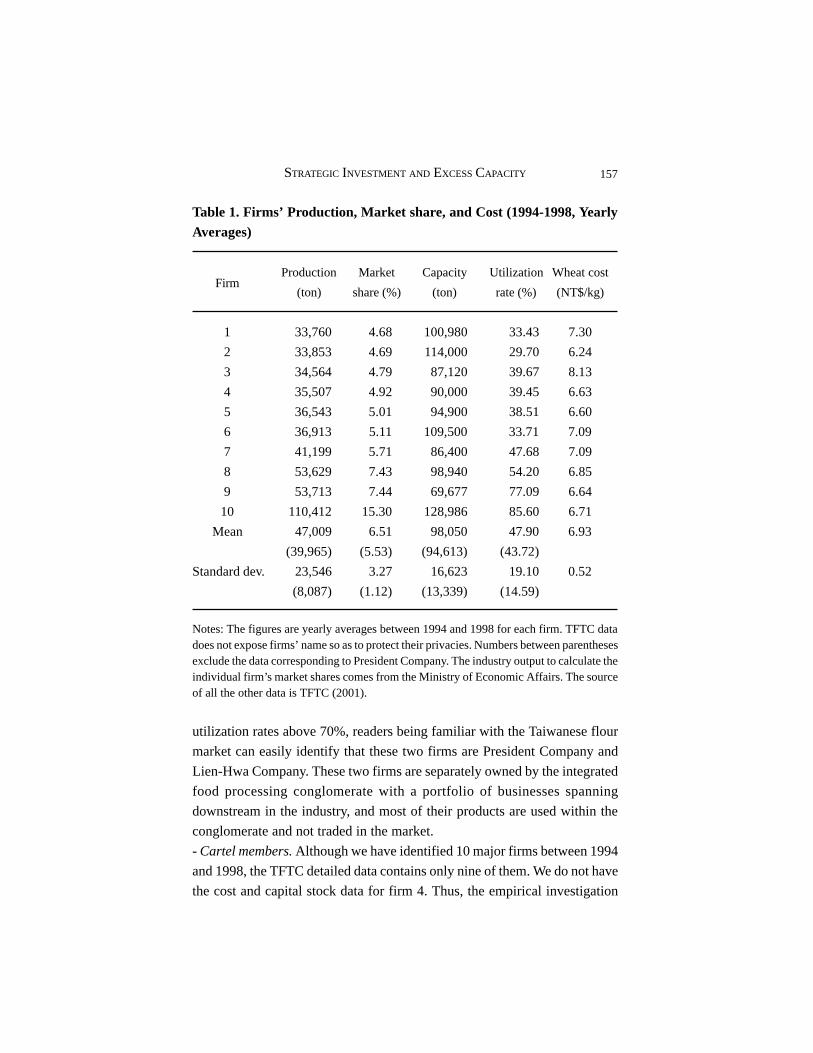
157STRATEGIC INVESTMENT AND EXCESS CAPACITY
Table 1. Firms’ Production, Market share, and Cost (1994-1998, YearlyAverages)
Production Market Capacity Utilization Wheat cost
(ton) share (%) (ton) rate (%) (NT$/kg)
1 33,760 4.68 100,980 33.43 7.30
2 33,853 4.69 114,000 29.70 6.24
3 34,564 4.79 87,120 39.67 8.13
4 35,507 4.92 90,000 39.45 6.63
5 36,543 5.01 94,900 38.51 6.60
6 36,913 5.11 109,500 33.71 7.09
7 41,199 5.71 86,400 47.68 7.09
8 53,629 7.43 98,940 54.20 6.85
9 53,713 7.44 69,677 77.09 6.64
10 110,412 15.30 128,986 85.60 6.71
Mean 47,009 6.51 98,050 47.90 6.93
(39,965) (5.53) (94,613) (43.72)
Standard dev. 23,546 3.27 16,623 19.10 0.52
(8,087) (1.12) (13,339) (14.59)
Notes: The figures are yearly averages between 1994 and 1998 for each firm. TFTC datadoes not expose firms’ name so as to protect their privacies. Numbers between parenthesesexclude the data corresponding to President Company. The industry output to calculate theindividual firm’s market shares comes from the Ministry of Economic Affairs. The sourceof all the other data is TFTC (2001).
Firm
utilization rates above 70%, readers being familiar with the Taiwanese flour
market can easily identify that these two firms are President Company and
Lien-Hwa Company. These two firms are separately owned by the integrated
food processing conglomerate with a portfolio of businesses spanning
downstream in the industry, and most of their products are used within the
conglomerate and not traded in the market.
- Cartel members. Although we have identified 10 major firms between 1994
and 1998, the TFTC detailed data contains only nine of them. We do not have
the cost and capital stock data for firm 4. Thus, the empirical investigation

158 JOURNAL OF APPLIED ECONOMICS
contains only the collusive behaviors among these 9 dominant firms, and the
remaining 23 firms are ignored. These dominant firms are hypothesized to
behave collusively to restrict output among them. In addition, the excess
capacity is used to restrict cheating within the dominant group. Since we
focus on dominant firms, and cheating probably happens, then the remaining
23 firms are implicitly irrelevant.
III. A Model of Competition for the Flour Industry
In this section, a two-stage game model is set up to deal with the competition
issue in flour market. The framework is inspired by Roller and Sickles (2000)
and Dixon (1986). Ma (2004b) also investigates the relationship between
strategic effects and conjectural variations under this framework. Flour firms
simultaneously decide the fixed factor input (capital stock) in the first stage
and then choose the variable factor input (such as wheat or labor) so as to
resolve quantity in the second stage. Thus, capital is treated as an endogenous
variable and is determined in the first stage, which affects both the production
cost and market competition in the second stage. This specification allows
for the possibility of a semicollusive market where firms compete in a long-
run variable, such as capital investment, and collude with respect to a short-
run variable, such as quantity or market share. For an individual firm, our
concern is about the effect of long-run capital investment on its rivals’ short-
run output decision.
We begin by specifying a quantity-setting game in which each flour firm
produces a homogeneous commodity and faces an inverse linear demand
function of the form:4
where P is the price and Q is the quantity demanded, and in equilibrium the
market quantity demanded equals the sum of the outputs of the individual
4 These assumptions could be justified by the technical structure of the industry that wementioned in section II. For instance, the output of industry is homogeneous and thewholesale price is uniform across firms. Therefore, the inverse demand function applieswell.
( ) ( )i JP Q a b q Q= + + (1)

159STRATEGIC INVESTMENT AND EXCESS CAPACITY
firms. Let there be n firms, each producing qi, such that
1
n
ii
Q q=
= ∑ is the industry
output, and n
J j ij i
Q q Q q≠
= = −∑ is the combined output of other firms.
Following Roller and Sickles (2000), we assume that cost structure is
used as a channel through which the first and the second stage decisions have
an effect on firms’ profitability. In the first stage (long-run), firms can vary
their cost through the adjustment in capital stock. However, in the second
stage (short-run), cost relies only on variable inputs, which is determined by
the quantity produced,5 given the capacity determined in the first stage. Thus,
the cost structure can be specified as follows:
where li is the variable factor input, LR
iC is the long-run cost function which
amounts to short-run cost ( )SR
iC plus fixed cost (r
i k
i). Note that, given a capital
stock ( )0i ik k= and a fixed capital price ( )0 ,i ir r= SR
iC is determined only by
qi, which is a function of l
i. In the second stage, firms choose l
i to determine
qi. However, in the first stage, capital turns out to be variable and firms can
change their cost by purchasing ki at a given price 0.ir
We now solve the two-stage game in a standard way. First, each firm
chooses li to maximize its profit in the second stage:
Given a predetermined capital level (k0), the short-run production cost of
firm i ( )SRi iC q is determined by the variable input l
i which gives the total
variable cost (wili) at a factor price w
i. Assuming that w
i is exogenously
determined, the first order condition for (3) is given by:
5 Thus, the cost in the second stage can be considered as the short-run variable cost.
( , ) [ ( ) , ]LR SRi i i i i i i i i iC q k C q l k r rk= + (2)
max ( ) ( )i
SRi i i i
lP Q q C qπ = −
0 0 0 0[ ( , ) ] ( , )i i i i J i i i i i iP q l k r Q q l k r w l= + −
(3)
(1 ) 0i ii i
i i
q qP b q w
l lθ
∂ ∂+ + − =
∂ ∂(4)

160 JOURNAL OF APPLIED ECONOMICS
where i
i
q
l
∂∂
is the marginal product of the variable input. Under the conjectural-
variation framework, Ji
i
Q
qθ ∂
=∂
is the conjectural variation. As stated earlier,
QJ is the output of other firms in the same industry.
If we were interested in both the existence and pattern of interdependence,
it would be adequate to allow each firm to have different conjectural variations.
However, as we are only interested in the existence of oligopolistic
interdependence, it is sufficient to evaluate the aggregate output response of
the other n -1 firms anticipated by firm i. Thus, following Roller and Sickles
(2000) and Farrell and Shapiro (1990), we assume that qi = q (i.e., that the
conjectural variation is the same across all the flour firms). In the special case
of Cournot behavior, q = 0. Furthermore, under perfect competition q = -1 ,
and under a perfect collusive solution, q = n - 1 . This provides a basis for
testing these hypotheses in the next section. We then rewrite (4) as:
Since the price of the variable factor is equal to its marginal revenue
product, we substitute ii
i
qw MR
l
∂= ×
∂into (5) and use the equilibrium condition
of an oligopoly market (MR = MCi). After some manipulations, the first order
condition (5) becomes
where ii
qs
Q= is the market share of the individual firm, and
Pb
Qε = − is the
price elasticity of demand. Equation (6) represents an oligopoly mark-up
formula that is customarily used to measure market power and is determined
by market share si, price elasticity e and market conduct parameter q.
Econometrically, q can be estimated as a free parameter and interpreted as
“the average collusiveness of conduct”. In the Cournot model, q = 0, the
mark-up expression is reduced to .i iP MC s
P ε−
= For perfect collusion or
(1 ) .ii
i
i
wP b q
q
l
θ− = − +∂∂
(5)
(1 ) ,i iP MC s
Pθ
ε−
= + (6)

161STRATEGIC INVESTMENT AND EXCESS CAPACITY
monopoly, the mark-up equals 1,
ε and for perfect competition it is zero. Since
,ii
i
qw MC
l
∂= ×
∂by using (4) and ( ),i JP a b q Q= + + the reaction function of
firm i is linear to the outputs of other firms, and we have:
where the slope of the reaction function is 1
.(2 )θ
−+
We now turn to the first stage of the game in which capital stock is
determined. It is noticeable that the firm’s equilibrium quantities defined by
the second-stage game are functions of its own capital and its rivals’ capital
in the first stage. Thus, the equilibrium outcome of the second stage can be
represented by * ( , ),i i Jq k K where KJ is the sum of the capital stocks of the
other firms. The fact that the capital is committed before the firm makes its
output decision implies that the firm can use its investment decision
strategically: the firm can influence its rivals’ outputs through its choice of
capacity. Given this specification, the profit of firm i in the first stage is:
Without loss of generality, we can omit the functional arguments “*” to
keep notation uncluttered. Thus, the corresponding first order condition for
each firm is given by
which could be rewritten as
Here, i
i
q
k
∂∂
is the marginal productivity of the capital, and J
i
Q
k
∂∂
is the strategic
( , , ) .(2 )
i Ji i J i
MC a bQq r Q MC
bθ
θ− −
= =+
(7)
* *max [ ( , ) ] ( , ) .i
i i i J J i i J i i i ik
P q k K Q q k K rk w lπ = + − −
[(1 ) ] 0i i Ji i
i i i
q q QP b q r
k k kθ∂ ∂ ∂
+ + + − =∂ ∂ ∂
[(1 ) ].
ii
i i i J
i i
qP r
k s q Q
P k kθ
ε
∂ −∂ ∂ ∂
= + +∂ ∂
(8)

162 JOURNAL OF APPLIED ECONOMICS
effect of firm i’s capacity on its rivals’ outputs. Formally, we should write this
strategic effect as [ ] ,eJ
i
Q
k
∂∂
since [ ]eJ
i
Q
k
∂∂
is firm i’s conjecture, or expectation,
about its rivals’ output responses for its capital investment. We assume that
J
i
Q
k
∂∂
is constant and is the same across the firms. In the subsequent empirical
work, we try to estimate J
i
Q
k
∂∂
to check if overinvestment is used to reduce the
output of rivals.
The economic significance of J
i
Q
k
∂∂
is evident if we bring the optimality
conditions of the first stage and the second stage together. The arrangement
could be done by substituting (6) into (8) and reducing (8) to,
Based on the propositions of Fudenberg and Tirole (1984) and Roller and
Sickles (2000), (9) can be decomposed into two effects. By changing ki, firm
i has a direct effect on its profit ,ii i
i
qr MC
k
∂− ∂
which is the effect of firm i’s
stage-one investment on its cost. This effect cannot influence the output of
firm j. On the other hand, the strategic effect J i
i
Q Ps
k ε ∂ ∂
results from the
two-stage specification that allows for the influence of firm i’s investment on
the output of firm j in the second stage. Whenever J
i
Q
k
∂∂
is zero, there is no
strategic effect, and (9) reduces to ,ki ii i i
i i
q qr MC MR MRP
k k
∂ ∂= = =
∂ ∂ which
corresponds to a one-stage simultaneous move quantity game. However, if
the strategic effect does exist and 0,J
i
Q
k
∂<
∂then the theoretical inferences
indicate a firm’s conjecture that a large capacity built in stage one can be used
strategically to reduce other firms’ outputs in stage two.
This strategic effect may come from different sources. For instance, in the
case of a cartel, the excess capacity could be used to discourage cheating
0.
Direct effect Strategic effect
i J ii i
i i
q Q Psr MC
k k ε∂ ∂
− + =∂ ∂
14243 14243
(9)

163STRATEGIC INVESTMENT AND EXCESS CAPACITY
behavior.6 This mechanism works through the channel that if cheating is
observed by the cartel, then all firms will produce at full capacity and revert
to competition. Subsequently, price collapses and many firms go bankrupt.
Thus, excess capacity could be used as a credible threat to enforce collusion,
and capital is endogenously determined in the first stage and affects the market
competition in the second stage. On the other hand, higher capacity can also
lead to lower short-run marginal cost, and thus to a smaller output by other
firms.7
Finally, in equation (9), 0J
i
Q
k
∂<
∂ means i
i ii
qr MC
k
∂>
∂under the oligopoly
equilibrium ( ),iMR MC= which implies that capital price (ri) is larger than
its marginal revenue of product ( ).kiMRP Thus, a small marginal product for
capital i
i
q
k
∂ ∂
caused by overinvestment in stage one leads to a misallocation
of resources in stage two.8
IV. Data, Empirical Specification and Estimation
- Data. As we have already mentioned in section II, TFTC (2001) contains
data about nine of ten major Taiwanese flour producers. The period that the
data set covered is between 1994 and 1998. Thus, we have 45 observations
for the regression analysis to be applied. The definitions of these variables
are listed in the Appendix. Basically, this article uses a set of panel data to
6 When there exists excess capacity, cartel members have an incentive to cheat and undercutthe collusive price, since they can take over a larger share of the market. Thus, traditionalIO theories believe that cartels break down for the sake of excess capacity. However, recentgame theoretic contributions, such as Osborne and Pitchik (1983, 1986, 1987) and Davidsonand Deneckere (1990), emphasize that the correlation between excess capacity and collusionis positive rather than negative.
7 This is a usual result proposed by Fudenberg and Tirole (1984), Bulow, Geanakoplos andKlemperer (1985), and Roller and Sickles (2000).
8 This result is consistent with the findings of Eaton and Grossman (1984), Yarrow (1985),Dixon (1986), and Roller and Sickles (2000). These models exhibit an asymmetry betweenk and l that leads to a non-optimal capital-labor ratio. Although production is efficient inthe short-run, the strategic use of capital makes firms be not on their long-run cost functions.

164 JOURNAL OF APPLIED ECONOMICS
test the collusive behaviors among the dominant firms. The panel data can be
useful in some issues. First, it provides more available data, and increases the
degrees of freedom. Second, combining both cross-section and time-series
data can lessen the problem that occurs in the case of the omitted variables.
- Empirical Specification. Econometrically, we should deal with the above
model by simultaneously estimating the demand function (1) and optimality
conditions (6) and (9) from supply side. This approach needs to specify a
linear demand function such as P = a + bQ + cZ, in which P is the flour price,
Q is the industry output, and Z is a set of exogenous variables, so that we
could estimate the elasticity of demand e. As the span of data covers only 5
years, demand elasticity becomes very difficult -if not impossible- to be
estimated. Thus, we have selected a plausible parametric value for demand
elasticity to implement the nonlinear regression analysis. We use 1.0 as the
demand elasticity in the baseline specification. Furthermore, in order to make
the model persuasive, a sensitivity analysis will be performed to check the
robustness of the empirical result.
Since the model has to be imbedded within a stochastic framework for
empirical implementation, we assume that both equations (6) and (9) are
stochastic due to errors in optimization, where eli and e
2i are error terms. We
now apply these two optimality conditions, obtained from the previous
theoretical framework, to test the market behavior of flour firms. First, rewrite
(6) as
Second, after some manipulations, (9) could be written as
Then, we differentiate reaction function (7) with respect to ki to get
1
1 (1 )
ii
i
MCP e
sθε
= +− +
(10)
1i
i i ii
J J
i i
q
k MC rs
Q QP Pk k
ε ε
∂∂
= −∂ ∂∂ ∂

165STRATEGIC INVESTMENT AND EXCESS CAPACITY
1,
2
i
i
J
i
q
kQ
kθ
∂∂
= −∂ +∂
and let J i
i J
Q k
k Qγ ∂
=∂
be the elasticity to measure the impact of the individual
firm’s investment on its rivals’ output. We therefore have:
Note that, in (10) and (11), .ii
qs
Q= Additionally, we have the following
identity:
Since these functional forms are non-linear and involve a set of
relationships, we have to use a non-linear simultaneous-equations model to
estimate the relevant coefficients. In addition, it is inevitable for the panel
data to involve the correlations of the disturbances across equations. If we do
not take into account these correlations between the disturbances of different
structural equations, we are not using all the available information about each
equation, and therefore we do not attain asymptotical efficiency. This
insufficiency can be overcome by estimating all equations of the system
simultaneously, using non-linear three-stage least squares.
- Empirical Results: Using these functional forms, we try to estimate the system
of three equations (10) (11), and (12), which endogenize firm’s capital stock
(ki), firm’s output (q
i), and industry output (Q), by non-linear three stage least
squares. The parameters to be estimated are q and g, and the regression results
are the ones that appear on Table 2.
The main result obtained is that the baseline specification (e = 1.0) generates
the expected sign of q and g. For the measurement of market power (q) there
are enough evidences to suggest that flour firms monopolize the market through
collusion. The estimated q is 7.58, which is significantly different form 0
2
1 1,
(2 )i i i
i iJ
MC rks e
P PQε ε
θ γ= − − +
+(11)
1
n
ii
Q q=
= ∑ (12)

166 JOURNAL OF APPLIED ECONOMICS
9 Since collusion happens in the second stage (market stage), using (6) is a standard approachto compute the price-cost margin. Please refer to Roller and Sickles (2000) for details.
10 We compute the mark-up for the case of Cournot-Nash behavior by setting q = 0.
(Cournot model) and -1 (perfect competition model). Since there are nine flour
firms in the sample, the result of q = 7.58 approximates to n – 1 = 8 under
collusive regime. This implies that we cannot reject the hypothesis that firms
do work out some forms of concerted actions to monopolize the market, and
therefore our empirical evidences support the decision made by the TFTC.
By substituting the mean value of si, the estimate of q and e = 1 into (6),9
the estimated mark-up over marginal cost is equal to 55.8%, which is
substantially higher than the 6.5% that would hold if the market followed a
Cournot-Nash behavior.10 We therefore have a 49.3% increase in the mark-up
due to the collusion in the market.
For the effect of strategic investment which determines whether a two-
stage setup can be reduced to a single-stage model, the result exhibits a negative
and significant g = -0.25. Capital stock being determined before the output
decision implies that an individual firm can use its investment decision
strategically. It conjectures that a 1% increase in capital investment could
reduce the outputs of its rivals by 0.25%. This encourages firms to increase
their capacity beyond the optimal level and, since new entry is artificially
precluded by the industry’s quota system, the excess capacity serves as an
instrument to discipline cartel members.
Empirical work by Rosenbaum (1989) also indicates that the correlation
Table 2. Empirical Results for Two-Stage Game, e e e e e = 1. Non-Linear Three-Stage Least-Squares Estimates
Coefficient Estimates Standard Deviation
q k7.58* 0.13
g - 0.25* 0.02
Notes: The estimate of g has been converted into an elasticity. The number of observationsis 45. * denotes that the estimates are significant at the level of 1%.

167STRATEGIC INVESTMENT AND EXCESS CAPACITY
between a firm’s excess capacity and other firms’ output is negative. High
level of excess capacity could be used to punish deviators more harshly, since
firms will easily dump a large amount of product into the market. The collusive
agreement can therefore be enforced by a threat to revert to the Nash
equilibrium strategies by fixing the prices in a non-cooperative game with
the same given capacity.
V. Sensitivity Analysis
- Specification of demand elasticity. Because of data limitation, we have
selected a specific parametric value for demand elasticity (e = 1.0) to implement
the nonlinear regression analysis. Basically, this approach is a mixture of
simulation and estimation, hence there will always be some arbitrariness in
the choice of demand parameters. In this section, we use sensitivity analysis
to examine the robustness of our findings to alternative parameterizations of
the demand elasticity. The results are presented in Table 3.
Two aspects of these results deserve comment. First, if e is larger than 0.8,
Table 3. Sensitivity Analysis
e q g
0.2 3,385.31 - 0.03*
0.4 5,588.78 - 0.06*
0.6 41,012.99 - 0.45*
0.8 8.13* - 0.23*
1.0 7.58* - 0.25*
1.2 5.09* - 0.23*
1.4 6.11* - 0.27*
1.6 7.12* - 0.30*
1.8 8.14* - 0.34*
2.0 9.15* - 0.37*
Notes: The estimate of g has been converted into an elasticity. The number of observationsis 45. * denotes that the estimates are significant at the level of 1%.

168 JOURNAL OF APPLIED ECONOMICS
the strategic effect (g) and the degree of collusiveness (q) have the expected
sign and are statistically significant. They are also robust to changes in e. The
estimated market conduct is between 5.09 and 9.15. All these estimated figures
are significantly different from zero (which is the corresponding Cournot-
Nash solution) and provide some evidences of cartel pricing.
Secondly, e and γ moving in the same direction implies that the strategic
effect is evident in the elastic part of the demand schedule. Since high e means
high price and low market output in the case of a linear demand, cartel members
have an incentive to cheat and undercut the collusive price so that they can
take over a larger share of the market. The cartel may therefore need a more
severe threat to sustain the collusive equilibrium. Thus, a stronger strategic
effect to induce excess capacity and to work out a credible threat is a necessary
condition for the success of the cartel. Under this situation, the cartel could
inflict on deviators a larger damage by producing up to its capacity.
In addition, the fact that values of q are insignificantly different form zero
when e is less than 0.8 indicates that a monopolist is always reluctant to set
price in the inelastic part of the demand schedule, because, if e is large enough,
even a considerably small value of iP MCP
− is consistent with collusion.
VI. Conclusion
In this paper, a two-stage game model is set up to deal with the strategic
effect of the firm’s capital investment on its rivals’ outputs. The model is
tested with panel data from the Taiwanese flour industry. The empirical
evidences show that oligopolists expect that the long-term effects of their
capacity investment may act to deter its competitors’ outputs. This leads to
overinvestment in the first stage and causes the misallocation of resources.
Besides, the estimate of the conjectural variations also implies that firms do
work out some forms of concerted actions to monopolize the market.
Appendix. Data Description and Construction
1) P: While there are some different grades of flour, output is homogenous
across producers for any given grade. For the same grade of flour, price
169STRATEGIC INVESTMENT AND EXCESS CAPACITY
therefore tends to uniformity. The variable P is constructed as a Divisia price
index for the three types of flour sold in the market.
2) MCi: Since the production technology of flour is simple and firms use a
common technology, it is both convenient and realistic to assume constant
marginal costs, particularly during periods of considerable excess capacity.
We also assume that the marginal cost comprises the wage cost, the material
cost and other expenses for production.
3) ki and q
i: The capacity of the individual firm (k
i) is an average of year
capacity. Production (qi) is the actual yearly production.
4) si: Market share is defined as .iq
Q5) r
i: Capital price is defined as r = k
P (r + d – g), where k
P is the price of the
capital, r is expected rate of return, d is the rate of depreciation and g is therate of capital gains. There are several ways to deal with g in the empirical
studies. In this article, we assume that flour firms do not care about the capi-tal gains when they decide to invest in the first stage. Thus, the capital price is
redefined as r = kP (r + d). Since Taiwan CPI increased only by an annual rate
of 2.6% between 1994 and 1998, we omit g in the user cost expression and
get r = kP r + k
P d.
6) The data of the opportunity cost (kP r ) is obtained from Ma (2004a). All
the other data comes from the TFTC (2001) data set.
References
Allen, Beth, Raymond Deneckere, Tom Faith, and Dan Kovenock (2000),“Capacity Precommitment as a Barrier to Entry: A Bertrand-Edgeworth
Approach,” Economic Theory 15: 501-530.Bulow, Jeremy, John Geanakoplos, and Paul Klemperer (1985), “Multimarket
Oligopoly: Strategic Substitutes and Complements,” Journal of Political
Economy 93: 488-511.
Chen, Tsiao-Wei (1986), “Issues on Grain Imports,” Economic Essays 2: 197-208, Taiwan Ministry of Economic Affairs, (in Chinese).
Davidson, Carl, and Raymond Deneckere (1990), “Excess Capacity andCollusion,” International Economic Review 31: 521-541.
Dixon, Huw D. (1986), “Strategic Investment with Consistent Conjectures,”
Oxford Economic Papers 38: 111-128.

170 JOURNAL OF APPLIED ECONOMICS
Eaton, Jonathan, and Gene Grossman (1984), “Strategic Capacity Investment
and Product Market Competition,” Discussion paper 80, Woodrow Wilson
School.
Fudenberg, Drew, and Jean Tirole (1984), “The Fat-cat Effect, the Puppy-
dog Ploy and the Lean and Hungry Look,” American Economic Review
74: 361-366.
Farrell, Joseph, and Carl Shapiro (1990), “Horizontal Mergers: An Equilibrium
Analysis,” American Economic Review 81: 107-125.
Ma, Tay-Cheng (2004a), “Disadvantage Collusion: A Case Study on Flour
Cartel,” Sun Yat-Sen Management Review (forthcoming, in Chinese).
Ma, Tay-Cheng (2004b), “Strategic Investment and Conjectural Variation,”
Fair Trade Quarterly (forthcoming, in Chinese).
Osborne, Martin J., and Carolyn Pitchik (1983), “Profit-sharing in a Collusive
Industry,” European Economics Review 22: 59-74.
Osborne, Martin J., and Carolyn Pitchik (1986), “Price Competition in a
Capacity-constrained Duopoly,” Journal of Economic Theory 38: 238-60.
Osborne, Martin J., and Carolyn Pitchik (1987), “Cartel, Profit and Excess
Capacity,” International Economics Review 28: 413-28.
Roller, Lars-Hendrik, and Robin Sickles (2000), “Capacity and Product Market
Competition: Measuring Market in a Puppy-dog Industry,” International
Journal of Industrial Organization 18: 845-865.
Rosenbaum, David (1989), “An Empirical Test on the Effect of Excess
Capacity in Price Setting, Capacity-constrained Supergames,”
International Journal of Industrial Organization 7: 231-241.
TFTC (2001), “The Concerted Behaviors in the Oligopolistic Market: A Case
Study on the Flour Industry,” Research Paper 9002, Taiwan Fair Trade
Commission (in Chinese).
Yarrow, George (1985), “Measures of Monopoly Welfare Loss in Markets with
Differentiated Products,” Journal of Industrial Economics 33: 515-530.
171EVALUATING TARGET ACHIEVEMENTS IN THE PUBLIC SECTOR
Journal of Applied Economics, Vol. VIII, No. 1 (May 2005), 171-190
EVALUATING TARGET ACHIEVEMENTS IN THEPUBLIC SECTOR: AN APPLICATION OF A RARE
NON-PARAMETRIC DEA AND MALMQUIST INDICES
JAMES ODECK*
The Norwegian University of Science and Technology and
The Norwegian Public Roads Administration
Submitted June 2003; accepted February 2004
This paper provides an assessment of the extent to which targets set by a public authorityare achieved by its operational units. A rare DEA framework and its subsequent Malmquistindices are applied on data comprising 19 units over a four year period of 1996 to 1999.The mean efficiency scores by which targets are achieved across the sample years aremoderate, in the range 0.81 to 0.93. Average productivity progress across the sample yearshas been 26 percent. The results illustrate the usefulness of DEA even when there are noinputs and the decomposable Malmquist index for productivity is an asset in exploringcauses of productivity growth.
JEL classification codes: L92, C61
Key words: target achievement, traffic safety, data envelopment analysis,
Malmquist indices
I. Introduction
Traffic safety has been a long time policy objective in most modern
countries and it is generally believed that compulsory vehicle inspections are
* Thanks are due to Harald Minken and Rune Elvik both at the Norwegian Institute ofTransport Economics for useful comments on an earlier version of this paper. I would alsolike to thank the Norwegian Public Roads Administration for funding this study. I am alsoindebted to two anonymous referees. Errors in this paper are of course mine and noneshould be attributed to the above named persons. Correspondence should be addressed toThe Norwegian University of Science and Technology, N- 7491 Trondheim, Norway orThe Norwegian Public Roads Administration, PO box 8142 Dep., N-0033 Oslo Norway.Email: [email protected].

172 JOURNAL OF APPLIED ECONOMICS
a necessary means for combating motor vehicle accidents. The underlying
rationale is that if vehicles and/or vehicle drivers meet certain standards and/
or certain degree of compliance with regulation accidents due to technical
failure or violation of regulation will be reduced. In fact compulsory motor
vehicle inspections are conducted in most countries of the world, often by
public agencies. Traditionally, the tasks of these agencies have been directed
toward passenger vehicles. In recent years, however, more attention is being
paid to heavy vehicles mainly due to two reasons. The first is that the proportion
of heavy vehicles in road traffic is increasing and hence the percentage of
heavy vehicles involved in motor vehicle accidents is also increasing. The
second is that the percentage of heavy vehicles involved in motor accidents is
still small but the rate of serious injuries and fatalities once they are involved
in accidents is high. Thus, increasing amount of resources is now being used
by agencies in heavy vehicle inspection services to enhance traffic safety. In
fact studies have shown that increased heavy vehicle inspections are
economically beneficial to the society at large as it generates benefits greater
than costs (Elvik, 1999).
One way of increasing the performance in heavy vehicle inspection
services, which the Norwegian Public Roads administration (NPRA) has
adopted since 1996, is to set targets that should be met by the regional
operational units involved in actual inspection services. The targets comprise
the number of different vehicles to be controlled categorised by the type of
control to be performed. Further, these targets are structured and designed to
promote the NPRAs objective of enhancing traffic safety.
A problem faced by the management of a public agency such as the NPRA,
however, is how to gauge the extent to which the targets set are met. A second
problem is how to evaluate the productivity by which the targets are being
met from one year to the other so as to gain insight on productivity
improvement or regress in services offered to the public.
This study has two related objectives. The first objective is to evaluate the
operating efficiency by which the operational units are able to meet or surpass
the targets set for them by NPRA. We accomplish this by, first a simple
descriptive analysis and then by applying a now well known linear
programming technique termed Data Envelopment Analysis (DEA) coined
by Charnes et al. (1978) for application in the public sector and non-profit

173EVALUATING TARGET ACHIEVEMENTS IN THE PUBLIC SECTOR
organisations where prices may be non-existent. The motivation for applying
DEA, like in many other previous studies, is that it is a powerful tool that can
easily aggregate performance indicators into one single performance indicator.
The second objective is to investigate the productivity by which the
operational units meet their objectives. The question addressed is the extent
to which operational units’ progress in meeting their targets as compared to
others facing the same conditions. We accomplish this by using the
Malmquist productivity index approach that originated from Malmquist
(1953) within a consumer context. Since the NPRA is part of the public sector
where economic behaviour is uncertain and there is no information on the
prices of services produced, Malmquist index based on DEA approach is
well suited for our case.
This paper is by no means the first to investigate target achievements by
means of DEA. A recent study on target assessments and which is appreciated
includes that of Lovell and Pastor (1997) where bank branch networks are
investigated. As far as we know, however, our study is the first study to evaluate
target achievements within the transport sector and in particular with respect
to road safety using DEA approach. Further, we contend that this is the first
study to investigate productivity growth in target achievements in the transport
sector, specifically using Malmquist indices. We note further that Odeck (2000)
conducted a study on the productivity growth in the Norwegian vehicle
inspectorate with data from 1989-91, but did not consider the target
achievement problem.
The remainder of this paper is organised into sections as follows. Section
II gives a brief summary of the target setting procedures, describes the
performance targets and provides a descriptive analysis of the ability of the
RRA’s to meet their targets. Section III introduces DEA approach used for
measuring target performance and its subsequent extensions to Malmquist
indices. In section IV, the empirical results are presented and discussed. The
final section contains concluding remarks and future extensions.
II. Target Setting Procedures and Data
As a means of enhancing road traffic safety at the national level, The
Norwegian Public Road Administration (NPRA) which is the national public

174 JOURNAL OF APPLIED ECONOMICS
roads authority in charge of traffic safety, sets performance targets to be met
by its regional operational units known as the Regional Road Agencies (RRA).The process of target setting proceeds by way of an instruction from the
General Director of the NPRA to the managers of the RRAs. The targetindicators are standardised and are the same for all the RRAs. The NPRAuses regional data, past experience, total resources accorded to the RRAs andother regional specific characteristics such as traffic volume etc as a basis fordiscussion. After 1996, the year when target setting was introduced, the NPRAhas had a norm that for each target the RRAs should at least meet their previousyear’s performance volumes for each indicator. At the end of each quarter,the RRA’s are informed on how well they perform through meetings betweenthe director general of NPRA and the managers of RRA’s. The data for ourstudy correspond to the annual periods of 1996 through 1999. Thus we evaluatethe annual achievements starting from 1996 and ending in 1999.
There are three indicators that are used for target setting within heavyvehicle inspections to enhance traffic safety and with which we are hereconcerned. These are:
1. Number of heavy vehicles controlled with respect to condition for usealong road sites and in companies.
2. Technical controls of heavy vehicles both in halls and along road sites.3. Seat belt controls along road sites for all vehicles including passenger
vehicles.Thus ultimately, the task of the operational units of traffic safety is to
perform inspections on heavy vehicles with the addition of safety or seatbelts controls also on passenger vehicles.
Our data set comprises 19 units covering all the autonomous regions inNorway. The success indicators cover the target values of all the threeindicators described above. We have converted each target value and achievedvalue to a single success indicator defined as percent of target value actuallyachieved. These are essentially pure numbers independent of the units in whichthe underlying indicators are measured and ranges from zero (an achievementof zero) to plus infinity where 100 imply exact achievements of targets. Thusan indicator above 100 implies that a target is surpassed.
A descriptive analysis of the target achievement by the operational unitsmay be obtained by exploring Table 1, where the results of target achievementsof the 3 indicators for all the 19 operational units of the NPRA are presented.

175E
VALU
AT
ING
TA
RG
ET A
CH
IEV
EM
EN
TS IN T
HE P
UB
LIC SE
CT
OR
Table 1. Target Achievements
1996 1997 1998 1999
(A) (B) (C) (A) (B) (C) (A) (B) (C) (A) (B) (C)
Mean 1.01 0.98 1.09 1.01 1.03 0.92 1.29 1.02 0.97 1.00 1.02 1.05
Min 0.88 0.73 0.75 0.69 0.63 0.53 0.86 0.63 0.52 0.56 0.59 0.69
Max 1.13 1.27 1.56 1.24 1.49 1.23 1.96 1.72 1.31 1.48 1.59 1.67
Std. dev. 0.07 0.12 0.21 0.14 0.18 0.17 0.35 0.24 0.21 0.18 0.18 0.21
Freq. dist.:
< 70 0 0 0 1 1 3 0 2 3 1 1 1
71-80 0 2 1 1 1 1 0 0 2 0 0 1
81-90 1 2 2 1 1 6 1 1 1 1 1 0
91-100 6 8 3 5 5 4 1 7 4 10 7 7
101-110 9 5 5 6 5 3 6 6 4 3 8 4
111-120 3 1 3 4 3 1 3 1 3 3 1 3
121-130 0 1 1 1 2 1 0 0 1 0 0 1
131-140 0 0 2 0 0 0 2 0 1 0 0 1
141-150 0 0 1 0 1 0 1 1 0 1 0 0
> 150 0 0 1 0 0 0 5 1 0 0 1 1
Notes: (A): Usage controls; (B): Technical controls; (C): Safety belt controls.

176 JOURNAL OF APPLIED ECONOMICS
The impression one gets from the mean of the data, with exception of
usage control in 1998, is that the majority of the operational units are proficient
at meeting their targets. Taking target by target, the mean achievement of
usage, technical and safety belt controls are in the range 1.01 to 1.29, 0.98 to
1.03, and 0.92 to 1.05 respectively. For the safety belt controls in particular, a
tremendous fluctuation is observed with 13 units exceeding targets in 1996,
only 5 in 1997, 9 in 1998 and 10 in 1999.
On target-by-target basis, the mean operational unit at worst comes within
14% percent of meeting the target. The standard deviation is observed to
first increase in the two first years and then to decrease or stabilize in the
final year. A explanation for increasing standard errors is difficult to give,
however, the fact that the standard errors are decreasing in the final year
may imply that targets, after their implementations have become tighter
eventually forcing units to be homogenous. Considering now the distribution
of achievements, it is observed that there is a concentration of units lying in
the range 91-110% of target achievement. There are few units below 91 and
above 111% although the variation is dependent on the target being
considered. We also reckon that some unit failed to meet their targets while
others managed to surpass their targets by a very large margin, a case that is
persistent throughout the years of observation. Since a high proportion of
units exceed their targets especially in the first year, this may suggest the
targets were too soft to start with.
The observations above however, depict mixed results. Some targets exhibit
larger variations than others as can be seen from the frequency distribution.
No general conclusion on the performance of the individual units can thus be
reached by the piecemeal approach above as performance varies by target
being considered. There is therefore a need for a model-based approach that
offers an aggregated measure of performance. Second, such a measure should
also be able to measure the productivity by which targets are achieved from
one year to another. We develop such a model in the next section.
One precaution is however, in order before proceeding. We are here
interested in measuring the efficiency and productivity by which targets set
by the NPRA are met assuming that these targets are set right and accurately
reflects the features of each operational unit’s environment. The NPRA could
not supply us with the data used to set targets (i.e. inputs are non-available)

177EVALUATING TARGET ACHIEVEMENTS IN THE PUBLIC SECTOR
due to confidentiality purposes. This is precisely what makes us use a rare
formulation of DEA, as the subsequent section will show. However, the
NPRA ensured us of the following which are essential for the analysis that
we carry out in the succeeding sections: (1) no inspection units were allotted
with increased resources in the period that we study and, (2) no units were
given softer targets i.e. the NPRA did not soften any targets in year t + 1
for any under achievements in year t. As explained by The NPRA, (2) is
currently maintained for the simple reason that the whole target setting
process will be evaluated in the year 2002. Combining (1) and (2) together,
the target-resource ratio of any of the units has been non-decreasing in the
sample year of study.
III. A DEA and Malmquist Based Analysis of Performance andProductivity Growth
The question that we pose is: are there any potential for efficiency
improvements and productivity improvements in targets achievement by the
NPRAs operational units and, if so, what are the magnitudes? To this end we
subject the data to a DEA analysis.
We thus assume that the operational unit managers attempt to maximise
the services that they provide. Further, we assume that the services they provide
consist of the indicators discussed in the preceding section. The denominators
of these indicators are assumed fixed and given by the NPRA. This assumption
of course ignores the possibility that the managers may sandbag so as to
minimise the possibility of receiving higher targets the following year. This
possibility is relevant but we ignore it as the NPRA could not supply us with
the relevant data. However, it offers future research possibilities, which we
hope to turn to in another study on the target setting procedures themselves.
The DEA formulation that we use in this study corresponds to the well-
known Banker et al. (1984) BCC formulation, but without inputs. For a
thorough treatment of DEA models without inputs or without outputs see a
recent paper by Lovell and Pastor (1999).
Let the vector of success indicators for the operational unit j be represented
by 1 3( ,..., ), 1,..,19.j j jy y y j= = Each element of yi is the ratio of an achieved
value to target value so that it is units-free. The assumption that the managers

178 JOURNAL OF APPLIED ECONOMICS
of the operational units maximise their success indicators leads to the following
linear programming problem,
subject to
where the optimal value of f denotes the performances indicator, i indexes thesuccess indicators, k indexes the operational units and l = (l
1,…, l
k,…, l
19) is
a vector of intensity variables and s+ik is the output slack variable.Note that in standard DEA model constraint (3) would imply variable
return to scale. Since there are no inputs, it makes the specification equal to aspecification with a constant input (Lovell and Pastor, 1999). The objective
of this problem is to maximize the radial expansion of the vector of successindicators for the operational units being evaluated. The constraints, i.e.
equations (2) and (3), limit this expansion to a convex combination of successindicators of other operational units in the sample. Thus the managers of the
operational units are here assumed to select a mix of success indicators thatvaries from one unit to another reflecting variation in location of the unit,
size and traffic volumes. The Maximization problem then determines theproportion by which the success indicators can be feasibly expanded in each
operational unit. A performance indicator for operational unit j is providedby the maximization above as the optimal value of f . Best practice performance
is identified in a unit that have output slacks s+ik = 0 and optimal f * = 1. Thisis because it is not possible to expand all success indicators equiproportionaly
without exceeding best practice observed in the sample. Units with optimalf * > 1 perform less than best practice ones. Thus an efficiency measure (E)
for a unit being evaluated can be readily derived as the inverse of the optimumvalue f *. An operational unit obtaining a score E = 1 will be technically efficient
while those with a score E < 1 will be technically inefficient.
, Max
φ λφ (1)
, 1,...,3ij ik ikk
k
y y s i φ λ +≤ − =∑ (2)
1kk
λ =∑ (3)
, 0 1,..., ,...,19ikk s k j λ + ≥ = (4)

179EVALUATING TARGET ACHIEVEMENTS IN THE PUBLIC SECTOR
Productivity and technical change between periods can be measured in
several ways. In this study we apply the Malmquist index. This index was
first presented in consumer theory by Malmquist (1953) and later for
productivity analysis by many e.g. Caves et al. (1982). The Malmquist index
has several advantages, which makes it suitable for our purpose. No assumption
regarding the economic behaviour of production units, e.g. cost minimisation
or revenue maximisation, needs to be made. Since the economic behaviour of
the operational production units of the NPRA is uncertain and there in no
price information on services produced, as often is the case for many public
sector bodies, the choice of Malmquist index is well justified.
The productivity growth1 in target achievement for an individual
operational unit can be measured by the Malmquist index as improved
efficiency relative to the benchmark frontier. Thus Malmquist index for
productivity growth can easily be expressed in DEA efficiency measures.
The Malmquist output based productivity index expressed in DEA output
measure for observation k between time periods t and t+1, based on the
technology at time t is,
i.e., the ratio between the output increasing efficiency measure for unit k
observed at time t+1 and t respectively, and measured against the technology
at time t. If M > 1 the productivity growth is said to have been positive. Note
that the base year can be any year. The Malmquist index above can be divided
into two components. The first component is known as the “catching up index”
and it shows the relative change in efficiency between the periods. The second
component is known as “frontier productivity index” and it shows the relative
distance between the frontiers i.e. measures the change of frontiers between
two periods. It is therefore sometimes referred to as the technical change
effect (see Färe et al., 1989; Berg et al., 1991; and Bjurek and Hjalmarsson,
1995). The decomposed Malmquist index is defined as,
1 In order to preserve terminology compatible with the traditional definition of Malmquistproductivity index, we use productivity growth to mean the same thing as change in targetachievement or target achievement index.
, ( 1),
, ( )
t k tt k
t k t
EM
E+= (5)

180 JOURNAL OF APPLIED ECONOMICS
1, ( 1) , ( 1), , ,
, ( ) 1, ( 1)
t k t t k tt k t k t k
t k t t k t
E EM MC MF
E E+ + +
+ +
= = ×
where MCt,k
is the catching up effect and MFt,k
is the change of the frontier
between time period’s t and t+1 for unit k. It follows from (6) that for a fully
efficient unit both years, MC = 1. In that case the index is a pure frontier
distance measure.
Unfortunately, like many indexes, Malmquist index is dependent on the
chosen reference technology. This may create a problem in the sense that the
circularity property of the indexes is not obeyed. To elaborate, assume that
we were evaluating the productivity growth between year t and t+1 but with
year t+2 as the base technology. In relation to equation (6), we now have
three technology periods t, t+1 and t+2. However, we see that if equation (6)
was to be applied directly, the frontier technology that we are measuring against
does not appear on the right hand side of the expression for frontier index.
Hence the Frisch circular relation is not obeyed and equation (6) is not
applicable (Frisch, 1932). The Malmquist index expressed can however be
adjusted to obey the circularity property. For a formal treatment and
applications see Berg et al. (1991), Bjurek and Hjalmarsson (1995) and Odeck
(2000). Since our data set comprise a short period of time where the interest
is to gain insight on productivity growth from when the target setting system
was introduced, we will base our analysis on a fixed reference technology
with 1996 as the base year. The decomposed Malmquist index for unit k with
fixed technology (f) and obeying the circularity property identical to equation
(6) is defined as (see Berg et al., 1991, and Bjurek and Hjalmarsson, 1995),
where Ef,k(t)
and Ef,k(t+1)
denotes the output increasing efficiency given the fixed
reference technology f at time t and t+1 respectively. When calculating the
productivity change for an entire period, Bjurek and Hjalmarsson (1995) have
proposed to use a fixed based index for period t = 1,…,T, as,
(6)
, ( 1)
1, ( 1) 1, ( 1), , ,
, ( ), ( )
, ( )
f k t
t k t t k tf k f k f k
f k tt k t
t k t
E
E EM MC MF
EE
E
+
+ + + += = × (7)

181EVALUATING TARGET ACHIEVEMENTS IN THE PUBLIC SECTOR
, ( 1)
1, ( 1) 1, ( 1),
, ( )1 , ( )
, ( )
f k t
Tt k t t k t
f kf k tt t k t
t k t
E
E EM MC MF
EE
E
+
+ + + +
=
= = ×∏
There are however, some drawbacks with the base period index used here (see
for instance Althin, 2001). If the base period is altered, the measurement of
productivity change will most likely be different as a direct result effect of the
base period alteration. The second drawback pertains to reference with a fixed
technology far a way in time. Here, the comparison with a technology far away
and has less or nothing in common with the current technology being evaluated,
may appear useless and strange. For this study, however, these problems may
be considered less relevant for the following two reasons. Firstly, we are
interested in investigating the change that occurred as a result of the introduction
of the targeting setting process. Base period index will thus give an indication
on how successful the regime introduced has been relative to the old one.
Secondly, the periods we consider are relatively short to expect tremendous
short and not far away in time i.e. data are from 1996 to 1999.
IV. Empirical Results
The data set at our disposal comprises target achievement indicators
described in section II. In Table 2 we present the summary results of the DEA
efficiency scores for each observation year as well as their frequency
distributions.
The mean efficiency declines from 0.93 in 1996 to 0.81 in 1999. The
same tendency is also observed for the least efficient unit, which declines
from 0.82 to 0.62 in 1996 and 1999 respectively. We however, observe the
reverse with respect to the spread around the mean which rises from 0.06 in
1996 to 0.14 in 1998 and then falls to 0.11 in the last year of observation.
Looking at the frequency distributions, it is observed that the number of units
in the interval 91-100 percent of efficiency is stable at 14 units in 1996 and
1997 then falls to only 4 units in 1999. Further, the total number of units
below efficiency score of 0.81 rises from zero in 1996 to 12 in 1998, and then
falls slightly to 10 in 1999.
(8)

182 JOURNAL OF APPLIED ECONOMICS
Table 2. Summary Results and Frequency Distribution of DEA EfficiencyScores
1996 1997 1998 1999
Mean 0.93 0.92 0.81 0.81
Min 0.82 0.65 0.57 0.62
Max 1.00 1.00 1.00 1.00
Std. Dev. 0.06 0.10 0.14 0.11
Freq. distribution (%):
< 70 0 1 3 2
71-80 0 1 9 8
81-90 5 3 1 5
91-100 14 14 6 4
A likely explanation to the observed falling trend in efficiency scores is
that in the first year when target setting procedure was introduced, many
units resorted to full utilisation of their potentials to achieve targets set for
them by the NPRA. Later, since there has not been any increase in resources
allotted to the operational units in the sample period of study, more and more
units had less unexploited resources which could be used to achieve the targets.
It should however, be borne in mind that the efficient units for each year
merely mean that these units performed best in the sample. It does not mean
or imply that they performed exceptionally well, or that they managed to
meet or surpass all or even most of their targets. Thus the efficiency scores
here only give an indication on how competitive the units are in achieving
their targets as compared to each other at every point in time.
It is of interest to investigate whether units maintain their relative positions
on the frontier from one year to the other. Some useful insight may be gained
by examining the overall distribution that is shown in Table 3.
There are fluctuations among individual units with respect to efficiency
scores from one year to the other. In terms of the number of frontier units
maintaining their relative positions, only 5 units appear on the frontier more
than one time and only 1 is on the frontier more than twice (unit no.19) when
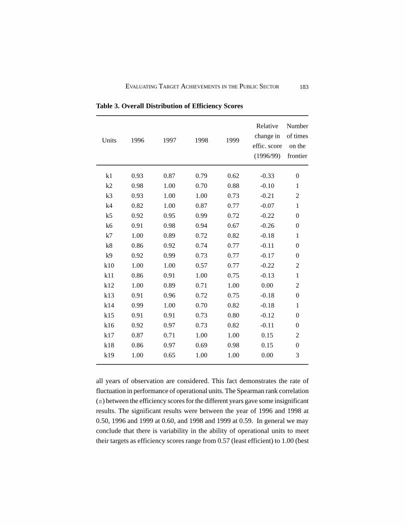
183EVALUATING TARGET ACHIEVEMENTS IN THE PUBLIC SECTOR
Table 3. Overall Distribution of Efficiency Scores
Relative Number
change in of times
effic. score on the
(1996/99) frontier
k1 0.93 0.87 0.79 0.62 -0.33 0
k2 0.98 1.00 0.70 0.88 -0.10 1
k3 0.93 1.00 1.00 0.73 -0.21 2
k4 0.82 1.00 0.87 0.77 -0.07 1
k5 0.92 0.95 0.99 0.72 -0.22 0
k6 0.91 0.98 0.94 0.67 -0.26 0
k7 1.00 0.89 0.72 0.82 -0.18 1
k8 0.86 0.92 0.74 0.77 -0.11 0
k9 0.92 0.99 0.73 0.77 -0.17 0
k10 1.00 1.00 0.57 0.77 -0.22 2
k11 0.86 0.91 1.00 0.75 -0.13 1
k12 1.00 0.89 0.71 1.00 0.00 2
k13 0.91 0.96 0.72 0.75 -0.18 0
k14 0.99 1.00 0.70 0.82 -0.18 1
k15 0.91 0.91 0.73 0.80 -0.12 0
k16 0.92 0.97 0.73 0.82 -0.11 0
k17 0.87 0.71 1.00 1.00 0.15 2
k18 0.86 0.97 0.69 0.98 0.15 0
k19 1.00 0.65 1.00 1.00 0.00 3
Units 1996 1997 1998 1999
all years of observation are considered. This fact demonstrates the rate of
fluctuation in performance of operational units. The Spearman rank correlation
(s) between the efficiency scores for the different years gave some insignificant
results. The significant results were between the year of 1996 and 1998 at
0.50, 1996 and 1999 at 0.60, and 1998 and 1999 at 0.59. In general we may
conclude that there is variability in the ability of operational units to meet
their targets as efficiency scores range from 0.57 (least efficient) to 1.00 (best

184 JOURNAL OF APPLIED ECONOMICS
practice unit) across all years of observation. Further, the mean efficiency
scores have fallen in the period of observation indicating that units are
experiencing difficulties in meeting their targets over time. Nonetheless, these
results should be of considerable interest to the managers of the NPRA who
want may know the magnitudes of potentials for improvement in target
achievements among its operational units. This information may be useful
when setting targets.
We now turn to evaluate the productivity growth in target achievement by
subjecting the data to a Malmquist index analysis as outlined in the preceding
section. In principle we could have used any year as the base year. However,
with only 3 periods (1996-97, 97-98 and 98-99) on hand, we find it more
interesting to explore the developments based on the first year of 1996 when
targets setting was first introduced.
The values for the fixed base indexes for the individual units calculated
using equation (8) are presented in Table 4. Values greater than one in the
table indicates progress; values less than one reflect regress in target
achievements.
For 17 operational units the catching-up index (MC) is a regress and only
two units show an unchanged catching-up index. The frontier shift index
(MF) is greater than 1 for all units suggesting that there has been a general
technological improvement among all units. The frequency distribution at
the bottom of the table summarizes these trends. These results show that some
units did not benefit from technological improvement. For instance, unit k16
experiences advancement in technological capacity but records diminished
efficiency improvement as measured by MC. The lagging performance in
efficiency outweighs technological improvement such that the total
productivity (M) fell across the sample year. A further example is unit k10
and k11 which simultaneously experiences positive technological advancement
and negative efficiency change which (on net) yield constant total productivity.
These examples clearly illustrate the advantages of the decomposable
productivity measure: the operational units perform differently in terms of
their ability to adapt to change.
The total productivity growth in target achievement for an average
operational unit shown in Table 5 is respectable at about 26 percent (score of
1.26) for the whole period i.e. from 1996 to 1999. Here we have taken the

185EVALUATING TARGET ACHIEVEMENTS IN THE PUBLIC SECTOR
Table 4. The Fixed Base Malmquist Productivity Index, Base Year 1996
Operational Total productivity Catching-up Frontier shift
units growth (M) index (MC) index (MF)
k1 0.99 0.98 1.01
k2 1.05 0.98 1.07
k3 0.99 0.98 1.01
k4 1.02 0.99 1.02
k5 1.00 0.98 1.01
k6 1.00 0.99 1.01
k7 0.97 0.94 1.04
k8 1.02 0.99 1.04
k9 1.00 0.98 1.02
k10 1.00 0.99 1.01
k11 1.00 0.99 1.01
k12 1.03 1.00 1.03
k13 0.99 0.98 1.01
k14 1.00 0.99 1.01
k15 1.03 1.00 1.03
k16 0.97 0.93 1.04
k17 1.83 1.15 1.59
k18 1.33 1.15 1.16
k19 1.15 1.00 1.15
Frequency distribution:
< 70 0 0 0
71-80 0 0 0
81-90 0 0 0
91-100 11 17 0
101-110 5 0 16
111-120 1 2 2
121-130 1 1 0

186 JOURNAL OF APPLIED ECONOMICS
Table 5. Mean Productivity Indices for the Average Unit
Year Total Productivity Catching-up Frontier Shift
Growth (Mf) Index (MC
f) (MF
f)
1996/97 1.01 1.04 0.97
1997/98 1.19 0.98 1.21
1998/99 1.04 0.97 1.07
1996/99 1.26 0.99 1.26
output-weighted means of our measures across units for each pair of year.
Looking at the developments on a period-by-period basis, productivity progress
is found to be 1, 19 and 4 percent for the periods 1996-97, 1997-98 and 1998-
99 respectively. The values for frontier shift index, which by definition
measures the technological innovation, shows the same trend. The catching-
up index which is the relative change in efficiency between the periods is
however, decreasing throughout the years of observation and is in fact a regress
after the period 1996/97. Thus a natural conclusion to draw here is that the
observed productivity growth is mainly due to technological improvements
among the operational units. A possible explanation for the observed
productivity growth for the average unit is that the target setting process
whereby the unit managers are collectively informed of their performances
has inspired some form of competition and the end result is productivity growth
in achieving targets. This improvement in productivity is manifested in
technological improvement - most likely explained by the fact that units have
found themselves forced to find new ways or methods of achieving targets.
The slow progress in the last period (1998-99) probably suggests that target
achievement based on last years performances without extra resources allotted
to the operational units might, after four years, be just getting close to its
point of saturation. This impression is strengthened by the observation in
Table 2 that the number of units obtaining efficiency scores in the interval 91
to 100 percent in 1999 has falls to only 4 units.
There are however, some deductions that may be drawn to help explain
the productivity results above. The NPRA informed us that there has not

187EVALUATING TARGET ACHIEVEMENTS IN THE PUBLIC SECTOR
been any increase in resource allocation to its operational units since 1996.
So when compulsory target achievement was introduced in 1996, the
operational units most likely utilised their otherwise idle factor inputs thereby
contributing to productivity progress. In the short-run, changes in the utilisation
of factor inputs are mainly reflected in catching-up component (MC), while
technological shift (MF) occur in somewhat longer time period. This is exactly
what we observe in the productivity indices above: in the very short period
we observe that there is an increase in the catching-up index (MC) while the
technological shift is a regress. Later we observe the reverse with a formidable
increase in technological shift. This suggests that units eventually found
production enhancing techniques and an example here could be better use of
the available manpower such as the right man at the right place. The
technological progress on the average outweighs the regress in efficiency as
measured by (MC) such that the overall productivity increases during the
sample period.
V. Conclusions and Future Extensions
A rare application of DEA and Malmquist indices has been used in this
paper to investigate target achievements of the operational units of the
Norwegian Public Roads Administration (NPRA) charged with traffic safety
services. The DEA framework applied corresponds to BCC model with a
unique constant input, or equivalently, with no input. We have thus been able
to provide an assessment of performance with limited data expressed only as
percentage of target achievement. The data set stretches across four years
starting from 1996.
From the data available we have been able to derive some useful insight
on the efficiency and productivity by which targets set by the NPRA are met
by the operational units. We have found the mean efficiency for the operational
unit to lie the interval of 0.81-0.93 depending on the year of observation.
There are however, some fluctuations among individual units with respect to
efficiency scores from one year to the other. These observations, especially
with respect to the ranking of units should be of interest to managers of the
NPRA as they reveal best practice performers.
The second finding concerns the productivity by which the operational

188 JOURNAL OF APPLIED ECONOMICS
units are able to meet their targets from one year to the other. On the average,
operational units have been productive in meeting their targets and the average
productivity across the periods has been 26 percent. A likely explanation for
the observed productivity progress is that, in the very short run operational
units have been able to utilise efficiently their resources (factor inputs) and
this is mainly manifested in the catching-up component of the Malmquist
index. In the somewhat longer run, units have been able to maintain and
improve the “state-of-the-art” technology. This study has also illustrated the
advantages of the decomposable productivity measure: the operational units
perform differently in terms of their ability to adapt to change. Factors such
as area of operation in terms of large cities or not and coastal area or not, does
not seem to impact on performance. We have here evaluated the efficiency
and productivity in target achievements in the Norwegian traffic safety sector
given the limited data available.
However, the results of this study should be interpreted with caution. The
study’s time span cover a period of 4 years, which rather too short a time for
anyone to draw robust conclusions on the productivity growth of any sector.
Nevertheless, the results presented here shed some useful light on how targets
are achieved in the sector considered.
Nonetheless, much work remains to be done. One area is to obtain
additional information on the specific characteristics of the operational units
such as the operating environment in which the units seek to meet their targets.
Such information would help explain the differences in target achievements
between units. Another area is to investigate the target setting procedures
themselves. The NPRA has not been able to supply us with extensive data
used in their target setting process. If available, such data would help in
exploring such things as scale efficiency as well as whether units are really
output maximizers or input minimizers. Further, with such information, we
would be able to carry out sensitivity tests as well as apply other competing
methods to efficiency measurement. This indicates that there are still some
future research directions in this field.

189EVALUATING TARGET ACHIEVEMENTS IN THE PUBLIC SECTOR
References
Althin, Rikard (2001), “Measurement of Productivity Changes: Two Malmquist
Index Approaches,” Journal of Productivity Analysis 16: 107-128.
Banker, Rajiv D., Abraham Charnes, and William W. Cooper (1984), “Some
Models for Estimating Technical and Scale Efficiencies in Data
Envelopment Analysis,” Management Science 30/9: 1078-1092.
Berg, Sigbjørn Atle, Finn R. Førsund, and Eilev S. Jansen (1991), “Technical
Efficiency of Norwegian Banks: The Non-parametric Approach to
Efficiency Measurements,” Journal of Productivity Analysis 2: 127-142.
Bjurek, Hans, and Lennart Hjalmarsson (1995), “Productivity in Multiple
Output Public Service: A Quadratic Frontier Function and Malmquist Index
Approach,” Journal of Public Economics 56: 447-460.
Caves, Douglas W., Laurits R. Christensen, and W. Erwin Diewert (1982),
“The Economic Theory of Index Numbers and the Measurement of Input,
Output and Productivity,” Econometrica 50: 1393-1414
Charnes, Abraham, William W. Cooper, and Eduardo Rhodes (1978),
“Measuring the Efficiency of Decision Making Units,” European Journal
of Operational Research 2: 429-444.
Elvik, Rune (1999), Bedre Trafikksikkerhet i Norge, Working paper no. 446,
Institute of Transport Economics, Norway.
Frisch, Ragnar (1932), “Annual Survey of General Economic Theory: The
Problem of Numbers,” Econometrica 4: 1-38.
Färe, R., S. Grosskopf, C. A. Knox Lovell, B. Lindgren, and P. Roos (1989),
“Productivity Development in Swedish Hospitals. A Malmquist Output
Index Approach,” in A. Charnes, W.W. Cooper, A. Lewin, and L. Seiford,
eds., Data Envelopment Analysis: Theory, Methodology and Applications,
Boston, MA, Kluwer Academic Publishers.
Lovell, C.A. Knox, and Jesús T. Pastor (1997), “Target Setting: An Application
to Bank Branch Network,” European Journal of Operational Research
98: 290-299.
Lovell, C. A. Knox, and Jesús T. Pastor (1999), “Radial DEA Models without
Inputs or without Outputs,” European Journal of Operational Research
118: 46-51.

190 JOURNAL OF APPLIED ECONOMICS
Malmquist, Sten (1953), “Index Numbers and Indifference Surfaces,” Trabajos
de Estadistica 4: 209-242.
Odeck, James (2000), “Assessing the Relative Efficiency and Productivity
Growth of Vehicle Inspection Services: An Application of DEA and
Malmquist Indices,” European Journal of Operational Research 126:501-514.
Schultz, John D, (1998) “Staying Alive,” Traffic World 255: 16 -18.

191NONLINEARITY IN THE RETURN TO EDUCATIONJournal of Applied Economics, Vol. VIII, No. 1 (May 2005), 191-202
NONLINEARITY IN THE RETURN TO EDUCATION
PHILIP A. TROSTEL*
University of Maine
Submitted February 2003; accepted May 2004
This study estimates marginal rates of return to investment in schooling in 12 countries.Significant systematic nonlinearity in the marginal rate of return is found. In particular, themarginal rate of return is increasing significantly at low levels of education, and decreasingsignificantly at high levels of education. This may help explain why estimates of the returnto schooling are often considerably higher when instrumenting for education.
JEL classification codes: I20, J24
Key words: return to education, nonlinearity, instrumental variables
I. Introduction
The rate of return to education has been estimated in literally hundreds of
studies (see the surveys by Psacharopoulos, 1985, 1994; Ashenfelter et al.,
1999; and Harmon et al. 2000). The vast majority of this work implicitly
assumes that the marginal rate of return is constant over all levels of education.
Some studies, however, found significant nonlinearity in the rate of return to
schooling. Most of this work focused on deviations from nonlinearity at
particular levels of education; that is, sheepskin effects (see, for example,
Hungerford and Solon, 1987; Belman and Heywood, 1991; and Jaeger and
Page, 1996). Perhaps as a result, evidence on the general nonlinearity in the
return to schooling appears inconsistent. Mincer (1974), Psacharopoulos
(1985, 1994), and Harmon and Walker (1999) showed significant diminishing
* Philip Trostel: Department of Economics & Margaret Chase Smith Center for PublicPolicy, University of Maine, Orono, ME 04469-5715; email: [email protected] constructive comments I am grateful to the editor, a referee, Ian Walker, and seminarparticipants at the University of Warwick.

192 JOURNAL OF APPLIED ECONOMICS
returns to education.1 Heckman and Polachek (1974), Card and Krueger
(1992), and Card (1995, 1999) argued that the rate of return appears roughly
constant. One could, however, interpret Card and Krueger’s (1992) results as
indicative of increasing returns at low levels of education. The results in
Heckman et al. (2003) suggest increasing returns at low levels of education
followed by diminishing returns at high levels of education. The general nature
of possible nonlinearity in the return to education is unclear.
This study tests for the general nonlinearity in the (private) rate of return
to education for working-age men using comparable micro data in 12 countries.
The data indicate that the marginal rate of return is essentially nil for the first
several years of schooling, it then increases rapidly until about year 12, and
then it declines.
II. Data
Data from the International Social Survey Programme (ISSP) are used.
The ISSP contains comparable cross-sectional data on individuals in 33
countries from 1985 through 1995 (most of the countries, however, only
participated in a few of the years). Only 13 of the countries have at least
1,000 observations of labor-market data for men, and measured schooling is
truncated between 10 and 14 in one of these countries (Great Britain). Thus
observations from Great Britain are excluded, leaving samples from 12
countries.
The 12 samples consist of men within the ages of 18 to 64; without missing
information on wage rates or education; and not self-employed, retired, or in
school. A handful of observations with more than 22 years of measured
education are also excluded.2 Table 1 lists for each country its: sample size,
number of cross sections, mean years of education, and standard deviation of
education.
1 Although not directly comparable to this literature, diminishing returns to schooling arealso suggested by the relatively high return to early interventions relative to later remedialinterventions (see Carneiro and Heckman, 2003).
2 The results are essentially invariant to either censoring or truncating the schooling data at20 years or any reasonable higher level.

193NONLINEARITY IN THE RETURN TO EDUCATION
Table 1. Summary Statistics
Country N Years S ss
West Germany 3,396 9 10.53 3.07
United States 3,347 11 13.54 2.90
Australia 3,090 6 11.64 2.78
Norway 2,751 7 12.52 2.97
Russia 2,537 5 13.09 3.39
Netherlands 2,215 6 13.21 3.72
Austria 1,755 8 11.01 2.57
Poland 1,456 5 11.07 2.66
Italy 1,347 6 11.87 3.89
East Germany 1,238 5 10.86 2.86
Ireland 1,176 6 12.10 3.07
New Zealand 1,126 5 12.69 3.14
III. Evidence of Nonlinearity
The equations to be estimated are simple nonlinear extensions of the
standard Mincer wage equation. That is, an education polynomial is used in a
log-wage equation rather than just a linear term:
where wi is the hourly wage rate of individual i, S is years of schooling, j is
the order of the education polynomial, E is potential experience (age minus
years of schooling minus six), h is the order of the experience polynomial
(following Murphy and Welch, 1990, this is a fourth-order polynomial), and
Y is a vector of indicator variables for each year.3
hj 'i 0 j i Eh Y i ii
ln(w ) S E Y= β + β + β + β + ε∑ ∑ (1)
3 Earnings are measured in categories in many of the countries. Thus, all of the resultsreported are from maximum-likelihood interval regressions. The results, however, areessentially the same for OLS regressions on category midpoints.
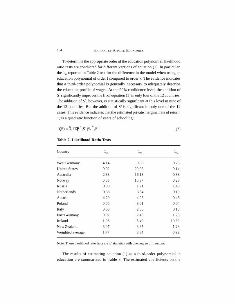
194 JOURNAL OF APPLIED ECONOMICS
To determine the appropriate order of the education polynomial, likelihood
ratio tests are conducted for different versions of equation (1). In particular,the l
kl reported in Table 2 test for the difference in the model when using an
education polynomial of order l compared to order k. The evidence indicatesthat a third-order polynomial is generally necessary to adequately describe
the education profile of wages. At the 90% confidence level, the addition ofS2 significantly improves the fit of equation (1) in only four of the 12 countries.
The addition of S3, however, is statistically significant at this level in nine ofthe 12 countries. But the addition of S4 is significant in only one of the 12
cases. This evidence indicates that the estimated private marginal rate of return,
r , is a quadratic function of years of schooling:
21 2 3
ˆ ˆ ˆˆ (S) 2 S 3 Sρ = β + β + β (2)
Table 2. Likelihood Ratio Tests
Country l12
l23
l34
West Germany 4.14 9.68 0.25
United States 0.02 20.06 0.14
Australia 2.33 16.18 0.33
Norway 0.05 10.37 0.28
Russia 0.00 1.71 1.48
Netherlands 0.38 3.54 0.10
Austria 4.20 4.06 0.46
Poland 0.06 3.01 0.04
Italy 3.68 2.55 0.10
East Germany 0.02 2.40 1.25
Ireland 1.06 5.40 10.39
New Zealand 8.07 8.85 1.28
Weighted average 1.77 8.84 0.92
Note: These likelihood ratio tests are c2 statistics with one degree of freedom.
The results of estimating equation (1) as a third-order polynomial ineducation are summarized in Table 3. The estimated coefficients on the

195NONLINEARITY IN THE RETURN TO EDUCATION
education polynomials are reported along with the implied marginal rates of
return for 8, 12, and 16 years of education (for comparison, estimates of the
standard linear rate of return are also shown). The equation (2) results are
illustrated in Figure 1 for West Germany and U.S.A.
4 Trostel et al. (2002) also use ISSP data. Their estimates of the rate of return are somewhatlower than the linear estimates in Table 3 because their estimation used an age polynomialinstead of an experience polynomial.
Figure 1. 95% Confidence Interval of the Marginal Rate of Return toEducation
West Germany United States
As emphasized in Trostel et al. (2002), there is considerable cross-country
variation in the linear rate of return to education.4 Yet there is considerable
cross-country similarity in the nonlinearity in the rate of return to education.
In all 12 countries the coefficient estimates on S and S3 are negative, and the
coefficient on S2 is positive. Moreover, 2β and
3β are statistically significant
with at least 95% confidence in eight of the 12 countries.
Although the levels of the estimates of the nonlinear marginal rates of
return to education vary considerably across countries, their nonlinear pattern
is quite consistent. ˆ (8)ρ and ˆ (16)ρ are lower than (12)ρ in all 12 countries.
Indeed, the marginal rates of return at 8 and 16 years of schooling are usually
substantially below those at 12 years. The weighted average ˆ (8)ρ and (16)ρ are
70.4% and 75.4% of the weighted average ˆ (12).ρ Moreover, the differences
in the estimated marginal rates of return are even greater at schooling levels
below 8 and above 16. The levels where the estimated marginal rates of return
reach a maximum lie in the narrow range between 11.5 and 12.9 years of

196 JOURNAL OF APPLIED ECONOMICS
Table 3. Rate of Return Estimates
Country 1β x 1022β x 103
3β x 104 ρ (8) ρ (12) ρ (16) Linearρ
West Germany -5.45 10.31 -2.91 0.06 0.07 0.05 0.06
(4.29) (3.47) (0.90) (0.01) (0.00) (0.00) (0.00)
United States -23.28 28.58 -7.59 0.08 0.13 0.10 0.10
(9.24) (7.21) (1.83) (0.02) (0.01) (0.01) (0.01)
Australia -14.43 18.99 -5.41 0.06 0.08 0.05 0.06
(3.83) (3.76) (1.17) (0.01) (0.01) (0.01) (0.00)
Norway -12.34 14.10 -3.65 0.03 0.06 0.05 0.05
(4.32) (3.50) (0.92) (0.01) (0.00) (0.00) (0.00)
Russia -6.71 9.53 -2.55 0.04 0.05 0.04 0.05
(7.38) (6.13) (1.67) (0.01) (0.01) (0.01) (0.00)
Netherlands -1.98 5.63 -1.53 0.04 0.05 0.04 0.04
(3.51) (2.83) (0.73) (0.01) (0.00) (0.00) (0.00)
Austria -7.90 13.13 -3.75 0.06 0.07 0.05 0.06
(6.78) (5.51) (1.42) (0.01) (0.01) (0.01) (0.00)
Poland -17.36 23.36 -6.77 0.07 0.10 0.05 0.08
(16.51) (14.60) (4.15) (0.02) (0.01) (0.02) (0.01)
Italy -3.03 8.09 -2.47 0.05 0.06 0.04 0.05
(6.79) (5.80) (1.55) (0.01) (0.01) (0.01) (0.00)
East Germany -21.67 19.95 -5.15 0.00 0.04 0.03 0.03
(13.39) (10.58) (2.71) (0.02) (0.01) (0.01) (0.00)
Ireland -6.89 16.07 -4.49 0.10 0.12 0.10 0.11
(10.30) (8.06) (2.08) (0.02) (0.01) (0.01) (0.01)
New Zealand -12.25 13.88 -3.43 0.03 0.06 0.06 0.05
(3.44) (3.42) (1.02) (0.01) (0.01) (0.01) (0.01)
Weighted average -11.34 15.41 -4.22 0.05 0.07 0.06 0.06
(6.82) (5.67) (1.52) (0.01) (0.01) (0.01) (0.00)
Note: Robust standard errors are in parentheses. The regressions include controls forpotential experience (fourth-order polynomial) and for each year.

197NONLINEARITY IN THE RETURN TO EDUCATION
education in all but two of the 12 countries. Even the two outliers in this
respect (10.9 years Italy and 13.5 years in New Zealand) are not far from the
others.
Thus, the evidence indicates that the marginal rate of return is increasing
significantly at relatively low levels of education, and decreasing significantly
at relatively high levels of education. Hence, linear estimates of the rate of
return (that is, weighted average marginal rates of return within countries)
noticeably understate the maximum marginal rates of return around 12 years
of schooling, and substantially overstate the rates of return at both the low
and high levels of education. Indeed, the return to investment in education is
insignificant for the first several years. Evidently, the initial increasing returns
in human capital production are substantial.
Because the marginal rate of return is lower at both ends of the education
distribution, a first-pass test for a non-constant rate of return does not reveal
much nonlinearity. The l12
in Table 2 are generally not significant (and the
coefficient estimates on S2 in a quadratic version of equation (1) are generally
not significant) because the initial increasing returns are offset by the later
diminishing returns.5
Various versions of equations (1) and (2) were estimated to check the
sensitivity of the nonlinearity in the rate of return.6 The nonlinearity results
were found to be robust. The marginal rate of return to education for women
displays a nonlinear relationship that is similar to men. Indeed, the nonlinearity
in the rate of return is somewhat more pronounced for women than men. The
results are essentially the same when using (log) monthly earnings as the
dependent variable rather than the (log) hourly wage rate. Similarly, the results
are essentially the same when using a second-order, instead of a fourth-order,
polynomial in potential experience (as is common in the literature). Similar
results are also found when using an age polynomial instead of a potential
experience polynomial. The nonlinearity results are unaffected when including
a schooling- experience interaction term, which allows for schooling to affect
5 Similarly, Box-Cox estimates of the relationship between w and S, such as in Heckmanand Polachek (1974), are extremely close to log-linearity (thus suggesting a near constantrate of return).
6 These results are available by request to the author.

198 JOURNAL OF APPLIED ECONOMICS
the experience profile of wages.7 The nonlinearity relationship remains, albeit
somewhat weaker, when dropping observations from either or both tails of
the education distribution. It is not just the extremes of the education
distribution that produce the estimated nonlinearity. A similar picture also
generally emerges when estimating equations (1) and (2) for ISSP countries
with less than 1,000 observations, and for each year separately.8
IV. Discussion
One problem with the above estimates of marginal rates of return is that
education is potentially endogenous. For this reason numerous recent studies
have used natural experiments as instruments to identify the causal effect of
education (see, for example, the recent survey by Card 1999). The ISSP,
however, does not contain good instruments for education. But even if there
were good instruments in the dataset, it is unlikely that they could yield
unbiased estimates of marginal rates of return. As stressed by Card (1995,
1999), typical instruments for education capture the causal effect of education
only at one point or over a small range of education outcomes. In the present
context where nonlinearity is explicitly examined, one needs valid instruments
for the entire range of education outcomes. Such instruments might not be
available in any dataset.
Moreover, the magnitude of the rate of return to education is not the primary
issue in this study. The issue is nonlinearity in the rate of return. Hence, the
primary concern in the present context is whether potential endogeneity of
7 The schooling-experience interaction coefficient is negative in nine of the 12 countries(i.e., the experience profile of wages usually flattens as education rises). Four of the ninenegative instances and two of the three positive cases are statistically significant (at 90%).In no instances, though, does the inclusion of the interaction term appreciably affect thenonlinearity in the rate of return.
8 A similar nonlinear relationship can also be found in larger datasets. Comparable estimatesfrom the U.K. Family Resources Survey in 1995 (N = 9,037) are 1β x 102 = -11.71 (5.05),
2β x 103 = 26.79 (4.00), and 3β x 104 = -8.88 (1.06). Comparable estimates from the U.S.Current Population Survey in 1991 (the last year that education was measured as years ofschooling instead of credentials) (N = 62,493) are 1β x 102 = 3.29 (0.92), 2β x 103 = 4.19(0.92), and
3β x 104 = -0.84 (0.28). Moreover, the nonlinearity in the CPS estimates occursdespite the measure of education being top-coded at 18 years.

199NONLINEARITY IN THE RETURN TO EDUCATION
education can explain the observed nonlinearity in the rate of return. It appears
that it cannot.
Endogeneity of education can potentially explain the rising rate of return
at the low end of the education distribution, but it works against observing a
declining rate of return at the high end. As again stressed by Card (1995,
1999), unobserved heterogeneity in ability, family background, etc. is likely
to cause schooling and wages to be positively correlated independent of the
causal effect of schooling. Thus, independent of the causal effect of schooling,
observed wages are likely to rise with the level of education. To the extent
that this is true, the observed marginal rate of return is rising with education
independently of its causal effect. The extent that this can explain the observed
rising return at low levels of education is, of course, unclear. In any event, the
direction of bias caused by this endogeneity is in one direction. Hence, it
cannot explain the observed diminishing returns at relatively high levels of
education.
Given that typical instruments for schooling capture the causal effect of
education only at small middle ranges in the distribution of schooling
outcomes, and that the (OLS) marginal rate of return is higher over the middle
range than over the entire education distribution; there is reason to expect IV
estimates of the rate of return to be greater than OLS estimates, a result
frequently found in the literature. This is essentially the problem stressed by
Card (1995, 1999), although in slightly different form. Card conjectured that
the marginal rate of return is declining throughout. Thus, instruments that
affect relatively low levels schooling will produce upwardly- biased estimates
of the average marginal rate of return. If, however, the marginal rate of return
is lower at both ends of the schooling distribution, then any instrument that
truncates this distribution toward the middle will yield an upwardly-biased
estimate of the average marginal rate of return, even those that affect relatively
high levels of schooling. Perhaps this can explain the finding in Harmon and
Walker (1999) that IV estimates are higher than OLS estimates even when
the instruments affect different schooling levels (a result that should not occur
if the marginal rate of return is declining throughout).
Another issue in the preceding empirical work is whether educational
sorting can explain the observed nonlinearity in the marginal rate of return.

200 JOURNAL OF APPLIED ECONOMICS
Although not completely decisive, there is considerable evidence that years
of education are sorted by ability, tastes, work attitudes, and so forth (e.g.,
Hungerford and Solon, 1987; Belman and Heywood, 1991; Kroch and
Sjoblom, 1994; Groot and Oosterbeeck, 1994; Weiss, 1995; and Jaeger and
Page, 1996). The preceding estimates subsumed possible sheepskin effects.
That is, the continuously-estimated nonlinearity could simply be reflecting
discrete changes at degree-completion years. This issue in this context,
however, is essentially the same as the possible endogeneity of schooling. In
particular, for essentially the same reason as above, educational sorting can
potentially explain at least some of the rising return at the low end of the
education distribution, but it works against finding diminishing returns at the
high end (unless there is some a priori reason for there to be sheepskin effects
at the secondary and undergraduate levels, while not at the graduate level).
V. Conclusion
Private marginal rates of return to education were estimated from
comparable micro data from 12 countries. Economically and statistically
significant nonlinearity was found in the return to education. Substantial
increasing returns were generally found in primary and secondary education.
Substantial diminishing returns were generally found in higher education.
Standard linear estimates of the rate of return to education substantially
overstate the marginal rates of return at both low and high levels of schooling,
and they noticeably understate the maximum rate of return at middle levels of
education.
The results also suggest that estimating the return to education is even
more problematic than perhaps previously believed. Using natural experiments
as instruments to identify the causal effect of education is particularly
problematic. Indeed, as argued by Card (1995, 1999), significant variation in
the marginal causal effect can explain why IV estimates of the rate of return
are usually noticeably higher than OLS estimates. Instruments that pick up
exogenous variation in education near the middle of the education distribution
(where the marginal causal effect is the highest) can be expected to yield
estimates of the rate of return greater than OLS estimates.

201NONLINEARITY IN THE RETURN TO EDUCATION
References
Ashenfelter, Orley, Colm Harmon, and Hessel Oosterbeek (1999), “A Review
of Estimates of the Schooling/Earnings Relationship, with Tests for
Publication Bias,” Labour Economics 6: 453-470.
Belman, Dale, and John S. Heywood (1991), “Sheepskin Effects in the Returns
to Education: An Examination of Women and Minorities,” Review of
Economics and Statistics 73: 720-724.
Card, David (1995), “Earnings, Schooling, and Ability Revisited,” Research
in Labor Economics 14: 23-48.
Card, David (1999), “The Causal Effect of Education on Earnings,” in O.
Ashenfelter and D. Card, eds., Handbook of Labor Economics Vol. 3A,
Amsterdam, Elsevier Science.
Card, David, and Alan B. Krueger (1992), “Does School Quality Matter?
Returns to Education and the Characteristics of Public Schools in the
United States,” Journal of Political Economy 100: 1-40.
Carneiro, Pedro, and James Heckman (2003), “Human Capital Policy,”
Working Paper 9495, Cambridge, MA, NBER.
Groot, Wim, and Hessel Oosterbeek (1994), “Earnings Effects of Different
Components of Schooling; Human Capital versus Screening,” Review of
Economics and Statistics 76: 317-321.
Harmon, Colm, Hessel Oosterbeek, and Ian Walker (2000), The Returns to
Education: A Review of Evidence, Issues and Deficiencies in the Literature,
London, Center for the Economics of Education.
Harmon, Colm, and Ian Walker (1999), “The Marginal and Average Returns
to Schooling in the UK,” European Economic Review 43: 879-887.
Heckman, James, and Solomon Polachek (1974), “Empirical Evidence on
the Functional Form of the Earnings-Schooling Relationship,” Journal of
the American Statistical Association 69: 350-354.
Heckman, James J., Lance J. Lochner, and Petra E. Todd (2003), “Fifty Years
of Mincer Earnings Functions,” Working Paper 9732, Cambridge, MA,
NBER.
Hungerford, Thomas, and Gary Solon (1987), “Sheepskin Effects in the Return
to Education,” Review of Economic and Statistics 69: 175-177.
Jaeger, David A., and Marianne E. Page (1996), “Degrees Matter: New

202 JOURNAL OF APPLIED ECONOMICS
Evidence on Sheepskin Effects in the Returns to Education,” Review of
Economics and Statistics 78: 733-740.
Kroch, Eugene A., and Kriss Sjoblom (1994), “Schooling as Human Capital
or a Signal,” Journal of Human Resources 29: 156-180.
Murphy, Kevin M., and Finis Welch (1990), “Empirical Age-Earnings
Profiles,” Journal of Labor Economics 8: 202-229.
Mincer, Jacob (1974), Schooling, Experience, and Earnings, New York,
Columbia University Press.
Psacharopoulos, George (1985), “Returns to Education: A Further
International Update and Implications,” Journal of Human Resources 20:
583-604.
Psacharopoulos, George (1994), “Returns to Investment in Education: A
Global Update,” World Development 22: 1325-1343.
Trostel, Philip, Ian Walker, and Paul Woolley (2002), “Estimates of the
Economic Return to Schooling for 28 Countries,” Labour Economics 9:
1-16.
Weiss, Andrew (1995), “Human Capital vs. Signalling Explanations of
Wages,” Journal of Economic Perspectives 9: 133-154.

203SUSTAINING FIXED RATES: THE POLITICAL ECONOMY OF CURRENCY PEGS
SUSTAINING FIXED RATES: THE POLITICAL ECONOMYOF CURRENCY PEGS IN LATIN AMERICA
S. BROCK BLOMBERG *
Claremont McKenna College
JEFFRY FRIEDEN
Harvard University
ERNESTO STEIN
Inter-American Development Bank
Submitted December 2004; accepted June 2005
Government exchange rate regime choice is constrained by both political and economicfactors. One political factor is the role of special interests: the larger the tradable sectorsexposed to international competition, the less likely is the maintenance of a fixed exchangerate regime. Another political factor is electoral: as an election approaches, the probabilityof the maintenance of a fixed exchange rate increases. We test these arguments with hazardmodels to analyze the duration dependence of Latin American exchange rate arrangementsfrom 1960 to 1999. We find substantial empirical evidence for these propositions. Resultsare robust to the inclusion of a variety of other economic and political variables, to differenttime and country samples, and to different definitions of regime arrangement. Controllingfor economic factors, a one percentage point increase in the size of the manufacturing sectoris associated with a reduction of six months in the longevity of a country’s currency peg. Animpending election increases the conditional likelihood of staying on a peg by about 8percent, while the aftershock of an election conversely increases the conditional probabilityof going off a peg by 4 percent.
JEL classification codes: D72, F31
Key words: exchange rates, elections
* S. Brock Blomberg (corresponding author): Department of Economics, Claremont McKennaCollege, e-mail [email protected]. Jeffry Frieden: Department ofGovernment, Harvard University, e-mail [email protected]. Ernesto Stein: ResearchDepartment, Inter-American Development Bank, e-mail [email protected]. We acknowledgethe extremely useful comments of Jorge Streb and two anonymous referees. We are alsograteful to Kishore Gawande, Carsten Hefeker, Michael Klein, Vladimir Klyuev, Chris Meissner,
Journal of Applied Economics. Vol VIII, No. 2 (Nov 2005), 203-225

JOURNAL OF APPLIED ECONOMICS204
I. Introduction
Government commitments to fixed exchange rates have been central to the
contemporary international political economy. In the context of European monetaryintegration, Latin American dollarization, Eastern European transition, the
stabilization of hyperinflation, and more, governments have attempted to peg their
currencies to those of other countries. In some cases, the attempts have beensuccessful – several Latin American countries have dollarized, and the euro now
exists. In more sensational cases, currency pegs have crashed with spectacular,
usually disastrous, consequences. The most recent Argentine economic andpolitical crisis began in 2001, when the authorities abandoned a decade-long
currency board arrangement that tied the peso to the dollar at a one-to-one exchange
rate. Russia’s dramatic 1998 crisis centered around attempts to support the ruble,and an eventual decision to let it depreciate massively. The East Asian crises of
1997-1998 similarly implicated currencies that were fixed either explicitly or implicitly
to the dollar; and the list could include dozens more countries over the past thirtyyears. These recent currency crises are in turn reminiscent of attempts, failed and
otherwise, of national governments to maintain their currencies’ links to the gold
standard in the interwar and pre-1914 period (Eichengreen 1992).The political economy of exchange rate commitments has however been little
explored by scholars. There is, to be sure, an enormous literature on the economics
of exchange rate pegs and currency crises (Sarno and Taylor 2002 survey theissues). There is also a very substantial normative literature on exchange rate
choice, dominated by variants of the optimal currency area approach, but its
conclusions are generally ambiguous – there are few unequivocal welfare criteriaupon which to base a choice of a peg, a floating rate, or some other policy.1 The
literature attempting to explain government exchange rate policies is much sparser.
Analysts have established that macroeconomic fundamentals by themselves cannotexplain exchange rate movements, but there is little agreement as to what additional
factors must be considered (Frankel and Rose 1995). There has been some study
J. David Richardson, Kenneth Scheve, Akila Weerapana; and participants in seminars atClaremont Mckenna College, Harvard University, New York University, Oberlin College, theUniversity of Michigan, University of Richmond and Syracuse University, and in panels at theannual meetings of the American Political Science Association and the Latin American andCaribbean Economic Association.
1 Tavlas (1994) is a good survey; Frankel and Rose (1998) argue for a somewhat less ambiguousview.

205SUSTAINING FIXED RATES: THE POLITICAL ECONOMY OF CURRENCY PEGS
of these issues in the context of European monetary integration and exchange ratepolicy in other industrialized regions, and some detailed empirical analyses of
particular experiences.2 Few of these explicitly consider electoral factors, or attempt
to evaluate both economic and political economy variables.3 Even fewer cross-national studies have looked at the developing-country experience, and their
incorporation of political factors is preliminary.4 There is a body of literature that
considers the choice of a fixed exchange rate in the context of monetary-policycredibility, but it is still small.5 And there are scattered studies of the political
economy of individual experiences with currency pegs, such as European monetary
integration, the Asian currency crisis, and the interwar period (for examples, seeEichengreen and Frieden 2001, Haggard 2000, and Simmons 1994 respectively).
There is a pressing need to understand both how politics mediates the impact of
macroeconomic factors on exchange rate decisions, and how politics affects suchdecisions directly.
This paper presents a political economy treatment of exchange rate regime
choice based on special-interest and electoral pressures. A government chooseswhether to stay on a fixed exchange rate regime or not; if it leaves the peg, it is
assumed to allow the currency to depreciate. A government’s willingness to sustain
a fixed rate depends on the value it places on the anti-inflationary effects of thepeg, as opposed to the countervailing value it attaches to gaining the freedom to
use the exchange rate to affect the relative price of tradables (“competitiveness”).
These arguments give rise to several propositions of empirical relevance. Thegreater the political influence of tradables producers, the less likely is the government
to sustain a fixed exchange rate regime. As an election approaches, governments
are more likely to sustain a currency peg, while they are more likely to abandon apeg once elected.
We test these implications with a large data base that includes information on
2 Eichengreen (1995) presents a general view; Edison and Melvin (1990), Hefeker (1996) and(1997), Frieden (1994) and (1997), Blomberg and Hess (1997), van der Ploeg (1989),Eichengreen and Frieden (1994), Frankel (1994), and Henning (1994) all present analyses ofparticular episodes or national experiences.
3 Bernhard and Leblang (1999) is a notable exception, as is Frieden, Ghezzi, and Stein (2001).
4 The most prominent such work includes Klein and Marion (1997), Collins (1996), andEdwards (1996). Two recent books, Wise and Roett (2000) and Frieden and Stein (2001), lookat the Latin American experience, largely with country case studies.
5 This work is represented especially by the articles in Bernhard, Broz, and Clark (2003).

JOURNAL OF APPLIED ECONOMICS206
economic and political characteristics of Latin American countries from 1960 to1999, using a hazard model to investigate the effects of both structural and time-
varying characteristics of these countries. We find that political and political
economy factors are crucial determinants of the likelihood that a government willsustain its commitment to a fixed rate. The more important is a country’s
manufacturing sector – which would be expected, in an open economy, to press for
a relatively weak currency and thus against a fixed rate – the less likely thegovernment is to be able to sustain a fixed rate. Electoral considerations, too, have
a powerful impact. Governments are more likely to abandon fixed exchange rate
regimes after elections, which is consistent with the idea that voters respondnegatively to governments that do not stand by their exchange rate commitments.
In addition, when currencies are seriously misaligned (appreciated), pegs are more
likely to be abandoned. The results are robust to the inclusion of a wide variety ofeconomic variables and specifications.
II. The argument
This section develops several propositions about the politics of exchange rate
regime choice, on which we base our empirical work on the duration of currencypegs. The focus is on a central tradeoff between “competitiveness” (defined as
the price of tradables relative to nontradables) and anti-inflationary credibility.
Sustaining a fixed exchange rate risks subjecting national producers to pressureon import and export markets, but has the advantage of moderating inflation.
Features of the national economic and political order affect the nature of the tradeoff,
and how it will be weighed by policymakers. In particular, tradables producers willoppose a fixed rate, so that a more politically influential tradables sector will lead
the government to be less likely to fix. At the same time, a principal advantage of
fixing for credibility purposes is to satisfy the broad electorate’s anti-inflationarypreferences, so that fixing will be more likely before elections than after them or in
non-election periods.
We start with several simple assumptions. First, we assume that the principaldecision facing the government is whether or not to peg its currency to a low-
inflation anchor currency. Second, we assume that a pegged currency will tend
toward a real appreciation (or at least that the danger will always exist with a peg),while a floating currency will tend to remain stable or to depreciate in real terms. In
the developing world, and particularly in Latin America, a history of high inflation
means that this has generally been the case. Indeed, Frieden, Ghezzi and Stein
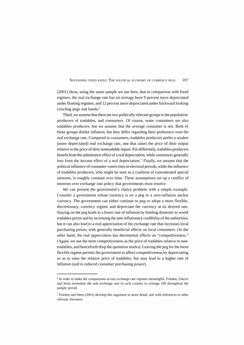
207SUSTAINING FIXED RATES: THE POLITICAL ECONOMY OF CURRENCY PEGS
(2001) show, using the same sample we use here, that in comparison with fixedregimes, the real exchange rate has on average been 9 percent more depreciated
under floating regimes, and 12 percent more depreciated under backward looking
crawling pegs and bands.6
Third, we assume that there are two politically relevant groups in the population:
producers of tradables, and consumers. Of course, some consumers are also
tradables producers, but we assume that the average consumer is not. Both ofthese groups dislike inflation, but they differ regarding their preference over the
real exchange rate. Compared to consumers, tradables producers prefer a weaker
(more depreciated) real exchange rate, one that raises the price of their outputrelative to the price of their nontradable inputs. Put differently, tradables producers
benefit from the substitution effect of a real depreciation, while consumers generally
lose from the income effect of a real depreciation.7 Finally, we assume that thepolitical influence of consumer-voters rises in electoral periods, while the influence
of tradables producers, who might be seen as a coalition of concentrated special
interests, is roughly constant over time. These assumptions set up a conflict ofinterests over exchange rate policy that governments must resolve.
We can present the government’s choice problem with a simple example.
Consider a government whose currency is on a peg to a zero-inflation anchorcurrency. The government can either continue to peg or adopt a more flexible,
discretionary, currency regime and depreciate the currency at its desired rate.
Staying on the peg leads to a lower rate of inflation by binding domestic to worldtradables prices and by increasing the anti-inflationary credibility of the authorities;
but it can also lead to a real appreciation of the exchange rate that increases local
purchasing power, with generally beneficial effects on local consumers. On theother hand, the real appreciation has detrimental effects on “competitiveness.”
(Again, we use the term competitiveness as the price of tradables relative to non-
tradables, and henceforth drop the quotation marks). Leaving the peg for the moreflexible regime permits the government to affect competitiveness by depreciating
so as to raise the relative price of tradables, but may lead to a higher rate of
inflation (and to reduced consumer purchasing power).
6 In order to make the comparisons across exchange rate regimes meaningful, Frieden, Ghezziand Stein normalize the real exchange rate in each country to average 100 throughout thesample period.
7 Frieden and Stein (2001) develop this argument in more detail, and with references to otherrelevant literature.

JOURNAL OF APPLIED ECONOMICS208
The government, faced with this tradeoff between credibility andcompetitiveness, makes its decision on the basis of political economy
considerations. We argue that the outcome will depend crucially on the relative
influence of tradables producers and consumer-voters. The influence of tradablesproducers is expected to have a negative impact on the likelihood that the
government will sustain a fixed exchange rate. The idea is simple: tradables
producers, harmed by a real or potential real appreciation, oppose the government’sgiving up the option of a currency depreciation to improve their competitive
position. Thus an increase in the political influence of tradables producers will
decrease the likelihood of staying on a currency peg.At the same time, inasmuch as politicians’ desire to address the concerns of
the more numerous consumer-voters rises near elections, the likelihood of sustaining
a currency peg is higher before elections than in post-election or non-electoralconditions. There are two interrelated reasons why this might be the case. First, an
anti-inflationary peg satisfies the interests of the general electorate in low inflation.
Second, a real appreciation increases general purchasing power, again in wayslikely to satisfy the interests of the general electorate. If other political and economic
factors make the peg difficult to sustain, of course, we should see an increase in
the probability of leaving the fixed exchange rate after an election.8 In other words,electoral periods will reduce the likelihood of abandoning exchange rate pegs.
In contrast, post-electoral periods will increase the likelihood of ending a peg.The argument made here also implies that government choice will be affected
by the starting point of the real exchange rate. If the initial exchange rate is severely
appreciated, its negative impact on tradables producers will be that much greater.
Thus a severe misalignment of the real exchange rate increases the concerns oftradables producers for competitiveness, and this will in turn increase the likelihood
of abandoning the peg. In other words, other things equal, political economy
factors make it more likely for a country with a relatively strong (appreciated)
real exchange rate to leave a currency peg. These three propositions can be
evaluated by looking at the empirical record of Latin American currency pegs to
the U.S. dollar, to see if such pegs are more likely to be sustained where tradables
8 It is not necessary to assume irrational voters for these implications to go through. There aremodels of rational voters, such as Rogoff (1990) and Rogoff and Sibert (1988), in whichelectoral cycles can be obtained as a result of a signalling game between the voters and thegovernment, in the context of asymmetric information. Stein and Streb (2004), and Bonomoand Terra (2005), are examples of this type of political budget cycle model focusing onexchange rate cycles.

209SUSTAINING FIXED RATES: THE POLITICAL ECONOMY OF CURRENCY PEGS
producers are weaker, before elections, and in the absence of a severe realappreciation.
III. Data and methodology
This section evaluates the evidence for our model in Latin America, using apanel of political and economic data developed by Frieden, Ghezzi, and Stein(2001). We begin with some descriptive statistics to introduce the data. We thendevelop a basic hazard model to determine the degree of duration dependence ofexchange rate regimes, and particularly currency pegs. We extend the model toinclude time-varying covariates, which allows us to sort out the importance ofpolitical variables in exchange rate determination.
A. Data description
We use data from 25 Latin American and Caribbean countries from 1960 to1999, drawn from IFS, the Economic and Social Database of the Inter-AmericanDevelopment Bank, and a variety of political sources (for more details see Frieden,Ghezzi, and Stein 2001). The data set covers every significant Latin American andCaribbean country except Cuba, and contains economic variables such as realexchange rates, GDP growth, inflation, the relative size of various sectors in theeconomy, along with a wide variety of political variables and a highly differentiateddefinition of exchange rate regimes. With regard to the political data, the data setincludes changes in government, elections, the number of effective parties, thegovernment’s vote share, political instability, and central bank independence.9
The definition of exchange rate regimes used allows for a more nuancedrepresentation of currency regimes than is common, classifying them on a nine-point scale.10 In most of what follows, in line with the argument, we collapse this
9 The variables included though not reported in the regressions include: changes in governmentdefined as dummy variables for all changes, and constitutional vs. unconstitutional separately;the number of effective parties is measured as the number of parties in the legislature updatedfrom Frieden and Stein (2001); central bank independence as the standard Cukierman measurealso from Frieden and Stein (2001); and liquidity as measured by central bank reserves over M2.
10 Formally, the exchange rate regime is defined as (see Frieden et al. 2001):REGIME
1 = 0 if fixed, single currency; 1 if fixed, basket; 2 if fixed for less than 6 months
(usually the case when authorities were not able to maintain fixed rate for a long enoughperiod); 3 if crawling forward peg (preannounced); 4 if crawling forward band (preannounced);5 if crawling backward peg (based on changes in some indicators – usually past inflation); 6 if

JOURNAL OF APPLIED ECONOMICS210
down to a 0-1 choice (with 1= fixed to a single currency, 0 otherwise) for our mainresults. That is, we define duration only in terms of currency regimes that involve
fixing to a single currency. However, following these results, we check whether the
results are robust to a broader definition of what constitutes a fixed exchange rateregime.
B. Preliminary data analysis
This section summarizes the exchange rate regime data. Figure 1 plots the
average REGIME1 aggregated across countries from 1960 to 1999. Recall that lower
numbers imply more fixed arrangements, while higher numbers imply more flexible
ones. Figure 1 shows very little time variation from 1960 until the end of the Bretton
crawling backward band (based on changes in some indicators – usually past inflation); 7 if dirtyfloating (floating regime with authorities intervening, or auctions at which Central Banks setthe amount of foreign currency to be sold or lowest bid, etc.); 8 if flexible.REGIME
2 = 1 if REGIME
1 = 0, 2, 3, 4; REGIME
2 = 0 otherwise.
Figure 1. Average exchange rate regimes
0
1
2
3
4
5
6
7
8
1960 1965 1970 1975 1980 1985 1990 1995 2000
Exc
hang
e ra
te a
rran
gem
ent
.
(0
to 8
sca
le: 8
mos
t fle
xib
le)
.

211SUSTAINING FIXED RATES: THE POLITICAL ECONOMY OF CURRENCY PEGS
Woods system in 1973. There was a gentle trend upward until the late 1980s, after
which there was a major shift toward floating. There are, of course, major differences
among countries.
Our model suggests that both elections and the political influence of the
tradables sector affect exchange rate regime choice. Table 1 presents suggestive
evidence. It shows the average size of the manufacturing sectors in Latin America
and the Caribbean, and the average exchange rate arrangement (using the broader
measure). Several of the countries with smaller manufacturing sectors are fixed
during the entire period in question, while none of the countries with larger
manufacturing sectors are. The average exchange rate regime is substantially more
flexible for economies with larger manufacturing sectors, and the six countries with
the most flexible regimes have large manufacturing sectors: Brazil, Colombia,
Uruguay, Peru, Chile and Mexico. We now turn to a more systematic evaluation of
the data.
Table 1. Size of manufacturing and exchange rate regime
Smaller manufacturing sectors Larger manufacturing sectors
MAN/ Scale of MAN/ Scale of
GDP fixed/floating GDP fixed/floating
Haiti 8.87 2.87 Dom. Republic 17.33 3.56
Panama 9.33 0.00 Venezuela 17.42 2.56
Barbados 10.12 0.00 Ecuador 19.37 2.12
Guyana 12.39 4.57 El Salvador 19.48 1.11
Trinidad & Tobago 12.61 2.46 Nicaragua 19.86 1.04
Suriname 13.82 1.87 Colombia 20.31 6.07
Guatemala 15.18 3.22 Chile 21.39 5.21
Honduras 15.24 2.57 Mexico 21.85 5.44
Paraguay 15.71 3.01 Costa Rica 22.83 3.86
Bolivia 16.03 4.32 Peru 23.47 5.21
Belize 16.65 0.00 Uruguay 23.66 5.48
Jamaica 17.22 4.05 Brazil 28.63 6.36
Argentina 29.35 2.47
Average 13.60 2.37 21.92 3.91
Note: Scale of fixed/floating is a 9 point scale with 0 = fixed for every period, 8 = floating for
every period.
Country Country

JOURNAL OF APPLIED ECONOMICS212
C. Basic empirical specification
The basic empirical model used here follows Greene (1997) and Kiefer (1988).
Previous research has analyzed exchange rate regimes by employing probit/logitanalysis to estimate the impact different factors have on the probability of being in
a given regime (Collins 1996, Klein and Marion 1997, Frieden, Ghezzi, and Stein
2001). While these papers provide very interesting results concerning the relativeimportance of different factors in influencing regime choice, they are not constructed
to directly analyze the sustainability of a regime. That is, they cannot directly
examine how likely a country is to remain in a regime, given that it has been in thatregime for a specified time. Hazard models allow us to analyze these issues directly,
by examining duration dependence, the likelihood that a country will abandon a
regime given that it has been in that regime for a specified time. A series is said tobe positively duration dependent if the hazard rate increases as the spell continues.
In our context, it means that a regime is more likely to end the longer a country has
been in it, while negative duration dependence means that the likelihood of leavingthe regime decreases as the time spent in it rises.
Put differently, our empirical methodology is based on a simple question –
given a currency peg at time t, will the country continue to peg its currency at timet+1? We evaluate the evidence empirically with a hazard model, whose natural
interpretation follows our argument. We can directly analyze the duration and
sustainability of regimes by defining them as “spells,” which allows us to examinethe “spell length” as a dynamic process such that the decision to remain on a peg
depends on previous decisions, and on other factors including our political economy
variables.The simplest version of our argument is deterministic, and predicts an
unambiguous regime choice. Even a small amount of uncertainty would allow us to
recast it in probabilistic terms. In this context, the impact of political factors onexchange rate regime duration would be expressed as increasing the likelihood of
abandoning a peg. Mathematically, we would be interested in examining the
likelihood, λ, of abandoning a regime at time t+1, given that the regime had notbeen abandoned at time t. This is a hazard rate, while the likelihood of survival of
a fixed exchange rate regime is a survival rate, inversely related to the hazard rate.
In either case the hazard model, as explained in greater detail below, is appropriateto examination of the durability of currency pegs.
We assume two possible regime arrangements, fixed and flexible. We define the
hazard rate, λ, as the rate that the spell in a fixed regime is completed at time t+1,

213SUSTAINING FIXED RATES: THE POLITICAL ECONOMY OF CURRENCY PEGS
given that it had not ended at time t. An intuitive representation of the hazard rate,λ, is the likelihood that the fixed regime survives. In this case, our hazard function
is merely the negative time derivative of a survival function S(t),
λ(t) = - d lnS(t) / dt.
Hence, whether we concentrate on the hazard or survival function, we candirectly observe the shape of the hazard/survival function and determine which
factors are important in causing the end of the fixed exchange rate regime conditional
on the fact that it had not ended previously. The hazard function is positivelyduration dependent at the point t* if dλ (t) / dt > 0 at t = t*, negatively duration
dependent at the point t* if dλ(t) / dt <0 at t = t*.
We originally considered various hazard models to include log-logistic, log-normal, and exponential among others.11 In each case, the general shape of these
different distributions turns out to be similar and so we extend the analysis in
future sections using the popular Weibull model. This is true when you considerboth the mean and median hazard rates.12 Hence, the qualitative results are robust
to alternative distributions of our hazard model.
The Weibull distribution’s hazard function is given by λp(λt) p-1 so that thereare two parameters θ = (λ,p) estimated in the simple model. In this case, the
probability, p, demonstrates whether the regime is positively duration dependent
(p>1), negatively duration dependent (p<1) or has no memory (p=1). We extractthese parameters by employing as a maximum likelihood estimation given by the
following likelihood function
ln L = Σ[δ λ(t |θ ) + ln S(t |θ )].
Note that there is right-censoring in many cases, as we do not observe the endof the last exchange regime as of 1999. In this case, we construct an indicator
variable δ, such that δ =0 for censored observations and δ =1 for the uncensored
observations.
11 The use of the Weibull model is not crucial for the results presented below. We consideredalternative specifications with qualitatively similar results. For simplicity and due to its widespreaduse, we only report the results for the Weibull specification.
12 Since the tipping point occurred significantly prior to the mean or median duration of pegs,we conclude that the choice of distribution is largely irrelevant.

JOURNAL OF APPLIED ECONOMICS214
D. The extended model with time varying covariates
The simple hazard model allows us to analyze the shapes of the hazard rates
and the duration dependence of the exchange rate regimes. The next step is toallow for different factors or covariates to influence the hazard rate. Now we describe
how we include covariates in general, without going into explicit detail. A formal
description of the time-varying covariate model is given in Petersen (1986).If we define the spell as the number of months on a peg and analyze each spell
as a unit (as we have thus far), we are excluding relevant information from the
empirical model. For example, suppose we wish to investigate the impact of inflationon duration and that the time in a given fixed regime is 24 months. It does not make
sense to include “average” inflation over the entire 24 months as a covariate, as
inflation changes on a month by month basis and we lose information in theaveraging. Similarly, it does not make sense only to include inflation in the initial
month, as the initial inflation rate is unlikely to be so important a determinant of the
duration of a regime two years later as the inflation rate at that point. It makes moresense to show how each monthly change in inflation affects monthly duration.
This can only be accomplished in a time-varying covariate framework. Hence, we
extend the analysis to allow for such time-varying factors by including thesecovariates as determinants in our hazard model, so that we estimate:
- ln λ = α + β X + ε,
where X is a vector of variables to include MAN/GDP, ELECTION, and political
and economic control variables and ε is our error term. This is the regressionestimated in our paper.
In doing so, we allow each individual monthly realization of our covariate (e.g.
inflation) to affect the hazard rate directly. If the spell ends, we calculate the impactof the individual country-month covariate on the duration. If the spell continues,
then we integrate these effects and allow them to continue to affect future duration.
Put differently, as time in a spell increases, each observation provides additionalinformation to the likelihood function. If the spell has ended, we calculate the
impact on the terminal point as in the baseline model; if the spell has not ended, we
sum these impacts and evaluate them at the end point. Taken together, we canconstruct parameter estimates from our likelihood function to calculate the impact
on spell length of these two separate sources: the direct impact if the spell is
terminated and the indirect impact from previous effects summed over the duration.

215SUSTAINING FIXED RATES: THE POLITICAL ECONOMY OF CURRENCY PEGS
In this way, we can think of the hazard function as a step function, with eachcovariate exhibiting different values through several intervals between the initial
and terminal point, when either censoring or exiting occurs. The model, then, has
an important dynamic component as both current covariates and previous durationaffect the hazard rate.
IV. Results
This section presents the results from estimating the model described above.
There are two main results. First, after a few months, there is substantial evidenceof negative duration dependence. The longer a country remains on a fixed exchange
rate, the less likely it is to leave the peg. Second, political-economy variables play
a major role in determining duration, as anticipated by the model. The size of themanufacturing sector, taken to indicate the political influence of tradables
producers, helps explain the hazard rate.13 So too does the timing of elections
affect the duration of currency pegs.
A. Explaining the duration of regimes
We begin by providing details from the basic hazard model discussed over the
time period 1972-1999 without covariates. This is interesting because it allows us
to unconditionally analyze the duration dependence of our exchange rate regimes.We find that we cannot reject the null that p<1, which implies negative duration
dependence – the longer a country has been on a currency peg, the less likely it is
to abandon it. We estimate median duration to be between three to five years(similar to the mean duration). The finding of negative duration dependence – that
pegs last longer as they endure – is in itself interesting. It may be that the longer
a peg lasts, the more wage and price-setting adjust to it and the easier it is tosustain. While these considerations are not inconsistent with our argument, they
lie outside it as currently formulated.
13 In other versions, we also included agriculture and mining as shares of GDP but found neitherto have an impact on duration. There are plausible explanations of the difference betweenmanufacturers and primary producers. Mining typically has substantial imported inputs, so thatthe real impact of a depreciation is mitigated. In Latin America, the agricultural sector isusually not very politically influential. In any case, we do not explore tradables sectors otherthan manufacturing further in this study.

JOURNAL OF APPLIED ECONOMICS216
Next we report the results from the model with time-varying covariates, whichestimates the impact of economic and political variables on the hazard rate. To
evaluate the political influence of tradables sectors concerned that a peg might
reduce their competitiveness we include manufacturing as a share of GDP [MAN/GDP], as manufacturers are likely to be particularly wary of forgoing the devaluation
option, and of the potential real appreciation associated with a fixed rate. We also
include a political dummy variable to capture electoral effects [ELECTION]. Thisvariable takes on the value -1 when an election was held in the previous four
months and +1 when an election is to be held in the next eight months. We expect
this variable to have a positive effect: a peg will be more likely to be sustained inthe runup to an election, and less likely to be sustained in post-electoral periods as
previous political business cycle incentives fade and pre-electoral appreciations
have to be unwound.14
Our next specification adds standard macroeconomic variables to the political
factors: GDP growth [DGDP], inflation [LN(INFLATION)] as a non-linear
determinant, the character of the international monetary regime as indicated by thepercent of countries that have fixed rates [INTL REGIME], and a measure of
openness as imports plus exports as a percent of GDP [OPENNESS]. The variables
DGDP and INTL REGIME should have a positive effect on the duration of a fixedregime, while we anticipate that inflation will have a negative effect. Duration
should rise if the economy is growing, as more countries adopt fixed rate regimes,
and with lower inflation.15 We are agnostic as to the variable OPENNESS:governments of more open economies might adopt a stable currency to encourage
trade and foreign investment, but they might also be more concerned about
competitiveness and therefore avoid a currency peg. We also include specificationsof each of the previous models that include country fixed effects to ensure that
results are not driven by country idiosyncrasies or that manufacturing is
endogenous to the existence of a peg. The results in Table 2 show that, indeed,they are not.
14 The construction of ELECTION is admittedly ad hoc, so we include results from tests thatthe coefficient associated with the pre- and post-election effects are statistically different fromone another. These tests show that there is no statistical difference in treating them separately,supporting our specification.
15 The inflationary impact may arise directly from monetary pressures or from politicalpressures that allow fiscal and monetary policies to follow inconsistent paths.

217SUSTAINING FIXED RATES: THE POLITICAL ECONOMY OF CURRENCY PEGS
Table 2. Explaining the duration of Latin American currency pegs, 1972-1999
Variable (1)=political (2) =(1)+economic(3)=(2)+misalign (4)=(3)+controls
Constant 7.254*** 6.667*** 7.045*** 5.633***
(0.764) (0.163) (0.807) (0.807)MAN/GDP -11.05*** -9.171*** -12.794*** -12.493***
(3.624) (1.063) (1.882) (4.456)ELECTION 0.552* * 0.275* 0.563* 0.570*
(0.270) (0.163) (0.319) (0.340)OPENNESS -1.314*** -1.002*** -1.050* *
(0.116) (0.391) (0.529)LN(INFLATION) -1.047*** -0.234 -0.327
(0.186) (0.146) (0.343)DGDP 13.467*** 25.850*** 25.737***
(4.014) (6.266) (8.705)INTL REGIME 1.839*** 1.630*** 1.509
(0.172) (0.605) (1.199)NX/GDP -0.024
(0.033)LN(GDP) 0.168
(0.541)I/GDP -0.002
(0.040)High Misalign -0.879* * -0.771
(0.511) (0.675)Low Misalign -0.324 -0.202
(0.453) (0.485)p 1.399*** 1.154*** 1.173*** 1.197***
(0.207) (0.174) (0.110) (0.167)
Chi-Sq(2) 4.23 3.21 2.38 2.33
P-value (0.12) (0.20) (0.30) (0.31)
pseudo R2 0.431 0.797 0.525 0.541
Notes: Column (1) includes political covariates as suggested by the model. Column (2) addsstandard economic variables as suggested by the model. Country fixed effects are included(though not reported). Column (3) adds misalignment variables and Column (4) adds furthereconomic controls. The row entitled Chi-Sq(2) is a test that the coefficients associated with thepre-election and post-election components of ELECTION are statistically different from oneanother. The row P-value reports the p-value associated with this test. Standard errors are inparenthesis and are clustered by country month cell. * is significant at 0.10 level, ** at .05 level,*** at .01 level.

JOURNAL OF APPLIED ECONOMICS218
16 We also considered other measures of misalignment, such as the top and bottom 10th and25th percentiles. In these different specifications, the impact of misalignments was notstatistically significant.
It will be recalled that the model leads to the expectation that when the realexchange rate is far from its target, a currency peg will be less likely to endure. To
evaluate this, in the final columns we add measures of severe real exchange rate
misalignment. These measures are dummy variables which takes a value of +1during periods of extreme appreciation or periods of extreme depreciation. The
exchange rate is considered misaligned when the country-month real exchange
rate is in the highest or lowest 5th percentile of all real exchange rate values usinga global notion of the real exchange rate [High Misalign, Low Misalign].16 The
variable is global in the statistical sense, so that it measures the most extreme
misalignments in the population of all misalignments. This approach allows forextreme misalignments to determine the sustainability in a manner independent of
the economic and political variables included in the regression. It also accounts
for possible non-linearities: in certain ranges there are no corrections, but if acertain threshold is surpassed there is pressure to correct the real exchange rate.
We anticipate that a severely appreciated real exchange rate will reduce the duration
of a peg, due to the pressure it places on tradables producers. We do not havestrong prior beliefs about the impact of a severely depreciated real exchange rate.
Finally, we provide a specification with other natural controls such as trade
imbalances [NX/GDP], real income per capita [LN(GDP)] and investment [I/GDP].We also examined many other possible variables, but do not include them in the
tables because of lost observations and for parsimony. In other specifications, we
considered time trends and dummies (which were significant but did not have adirect interpretation and did not change any of the other results), measures of
capital controls (insignificant), broad measures of liquidity (insignificant), central
bank independence (insignificant), political instability (insignificant) andgovernment change (insignificant when ELECTION is included).
Table 2 provides the results for the baseline hazard model from 1972 to 1999,
restricting the sample to this period because there was very little variation inregimes during the Bretton Woods years. Column (1) reports the results for the
model with political variables, Column (2) reports the results for the model with
political and economic variables. In Column (3) we add the measures ofmisalignment, and in Column (4) we add macroeconomic controls.
In all cases, the coefficients on the political variables are significant and have
the expected sign. MAN/GDP has a strong negative influence on duration; the

219SUSTAINING FIXED RATES: THE POLITICAL ECONOMY OF CURRENCY PEGS
larger the industrial sector, the less likely is a fixed exchange rate regime to endure.Pre-electoral and post-electoral shocks together affect regime choice in the manner
suggested by the model. The political variables continue to perform as predicted
by the model after economic variables are added, and with fixed effects. Mosteconomic variables perform as expected. Stronger GDP growth and lower inflation
increase duration. The global prevalence of fixed exchange rates increases the
duration of a fixed exchange rate regime (INTL REGIME is positive). On the otherhand, more openness seems to decrease duration. This somewhat surprising result,
repeated in other studies, may be due to the greater concern of open economies
about competitiveness and speculative attacks; we leave this issue for furtherresearch. When we include measures of extreme misalignment along with the
variables, in Column (3), it is clear that a substantially appreciated (“overvalued”)
real exchange rate reduces the duration of a peg, while an “undervaluation” has noimpact. The inclusion of the real exchange rate misalignment measures does not
appreciably affect the other economic or political variables.
These results allow us to describe the actual economic significance of thevariables of greatest interest. As we estimate p close to 1, the model can be collapsed
to an exponential one. In this case, a one percent increase in MAN/GDP translates
into a 10-12 percent decrease in the median duration of a regime, which amounts tosix months. This means that an increase in the size of the manufacturing sector of
just one percentage point reduces the expected duration of a peg by six months. It
is also instructive to consider how this affects the hazard rate directly. In this case,a one percent increase in the manufacturing share of GDP translates to a 10-12
percent increase in the hazard rate, the rate at which spells are completed after
duration t, given that they last at least until t. This means that an increase in thesize of the manufacturing sector of just one percentage point increases the
conditional likelihood of the peg ending by roughly 10-12 percent. Since the
manufacturing share of GDP is likely to vary primarily across countries, or overrelatively long periods of time, it is probably most enlightening to think of this as
a finding that the size of a country’s manufacturing sector as a share of GDP has a
very large negative impact on the likelihood that a currency peg in a country will besustained. The standard deviation of MAN/GDP for the sample is 5.5 percent; a
one standard-deviation increase in the share of manufacturing in the economy
reduces the expected length of a peg by 33 months, and reduces the conditionalprobability that a peg will be maintained by 66 percent. Put differently, exchange
rate pegs are likely to be 10 years shorter in Argentina than in Panama just due to
the differences in the role of manufacturing in these two countries. This is fully in

JOURNAL OF APPLIED ECONOMICS220
line with the expectations of the model. The fact that manufacturing, but not suchother tradables sectors as mining and agriculture, has such an impact is interesting,
and undoubtedly reflects both economic and political differences among tradables
sectors. We do not explore this further here, but it suggests directions for futureresearch.
We can similarly estimate the impact of elections. During a month in which an
election is pending, there is a one percent increase in the median duration of acurrency peg, equal to half a month. By the same token, for every month after an
election the expected duration of the peg decreases by about half a month. These
results imply that during the eight months prior to an election, the duration of acurrency peg is extended by about four months, while during the four months
following an election, a peg’s duration is reduced by about two months.17 Expressed
differently, the impact of an election next month decreases the hazard rate by 1percent (a 1 percent decrease in the conditional likelihood of the peg ending)
whereas past elections increase the hazard rate by 1 percent (a 1 percent increase
in the conditional likelihood of the peg ending). Taken together, the results onelection timing imply that during the eight months prior to an election, the
conditional likelihood of the peg ending is reduced by 8 percent, while during the
four months following an election, the conditional likelihood of a peg ending isincreased by 4 percent. One implication of this result is that pegs that survive pre-
election and post-election periods without deviating from a peg have an increased
chance of survival, ceteris paribus. Both the size of the manufacturing sector andelection timing, then, have statistically significant and economically important
effects on the duration of fixed exchange rate regimes. These results tend to confirm
the expectations of our model.18
B. Sensitivity analysis
Here we attempt to see if our results are sensitive to different specifications,
and different definitions of the complex data used in our analysis. We start by
17 The timing of the pre- and post- electoral dummy was selected by the specification whichmaximized the likelihood function. Small changes in the timing do not greatly influence theresults.
18 Alternatively, one might expect electoral cycles to be more important in countries with largemanufacturing sectors. As an experiment, we included an interaction term of ELECTION*[MAN/GDP] but found there was no statistical significant impact from the interaction term and theindividual terms, ELECTION, and MAN/GDP.

221SUSTAINING FIXED RATES: THE POLITICAL ECONOMY OF CURRENCY PEGS
Table 3. Explaining the duration of Latin American currency pegs: Sensitivityanalysis using different scales and different years
(1) Narrow (2) Broad (3) Broad (4) Narrow (5) Reinhart Variable definition definition definition w/o outliers & Rogoff
1960-1999 1972-1999 1960-1999 1972-1999 1972-1999
Constant 6.841*** 6.844*** 6.322*** 6.329*** 5.812***
(0.903) (0.969) (0.622) (0.969) (0.617)MAN/GDP -12.242*** -12.374*** -11.080*** -10.950* * -6.028* *
(3.874) (4.101) (2.432) (2.34) (2.94)ELECTION 0.601* 0.592* 0.652*** 0.620* 0.430* *
(0.352) (0.323) (0.222) (0.369) (0.181)OPENNESS -0.904*** -1.049*** -0.725* * -0.951* * 0.977
(0.426) (0.41) (0.339) (0.443) (0.744)LN(INFLATION) -0.276 -0.257 -0.235 -0. 228 -0.593***
(0.337) (0.32) (0.159) (0.346) (0.214)DGDP 28.44*** 25.79*** 22.80*** 26.97*** 10.577
(8.74) (8.3) (5.92) (9.03) (7.15)INTL REGIME 1.901* * 1.627 1.879* * 1.958* -0.262
(0.821) (1.231) (0.532) (1.11) (0.305)High Misalign -1.171* * -0.905 -0.791* -0.902 -0.422
(0.573) (0.559) (0.41) (0.599) (0.353)Low Misalign -0.368 -0.359 -0.372 -0.209 -0.152
(0.462) (0.438) (0.35) (0.471) (0.261)p 1.059*** 1.166*** 1.177*** 1.062*** 2.193***
(0.137) (0.15) (0.109) (0.144) (0.617)
pseudo R2 0.624 0.512 0.805 0.531 0.606
Notes: These specifications are variants of Column (3) in Table 2 that include political,economic and misalignment variables. Column (1) employs the same narrow definition over alonger time sample. Columns (2) and (3) employ more broad definitions of pegs over differenttime samples. Column (4) excludes four countries that had fixed exchange rates throughout theentire sample. Column (5) employs Reinhart & Rogoff ’s (2002) measure of de facto peggedexchange rates with bands widths +/-2% or less. Standard errors are in parenthesis and areclustered by country month cell. * is significant at 0.10 level, ** at .05 level, *** at .01 level.

JOURNAL OF APPLIED ECONOMICS222
19 We substitute Reinhart and Rogoff’s measure in place of our measure where available. Weemploy their classification of 9 or less, which corresponds with bands +/-2% or narrower.
varying the definition of a fixed-rate regime. The data, in fact, differentiate amongnine different exchange rate regimes, ranging from 0 to 8, with 0 most fixed and 8
most flexible. In previous specifications, only the lowest category, of currencies
unambiguously fixed to a single currency, was considered to be a fixed rate. Weexpand the definition of a fixed rate to include currencies fixed for relatively short
times, and currency pegs or target zones set by forward indexing, commonly known
as tablitas in Latin America, which are usually adopted for anti-inflationary reasonssimilar to those of fixed rates (these are categories 0, 2, 3, and 4 in the scale). We
also check the robustness of the results by extending the sample back to 1960, and
we experiment with dropping outliers.The sensitivity analysis is reported in Table 3. The results reported here are
quite similar to Table 2, although the coefficients are generally slightly smaller.
When we extend the analysis to 1960-1999, as in Column (1), the impact of MAN/GDP and ELECTION continue to be of practically the same magnitude and precision.
In Columns (2) and (3) we employ the broader definition of regime and find very
similarly strong effects from MAN/GDP and ELECTION. We then dropped fromour sample four countries that were pegged throughout the sample. As reported in
Column (4), we continue to find statistically strong results of similar magnitude.
The standard errors are slightly larger, but this may be due to the omission ofobservations from our outliers. In our final check, we employ Reinhart and Rogoff’s
de facto measure of fixed exchange rates in lieu of our measure.19 Once again, the
signs of the coefficients associated with MAN/GDP and ELECTION conform withour theory and are statistically significant. In this case, LN(INFLATION) is
statistically significant and p is closer to 2 than 1. This is probably because de
facto exchange rate regimes are, by definition, shorter in duration and are moresensitive to inflation.
V. Conclusions
This paper argues that government policy toward the exchange rate reflects a
tradeoff between the competitiveness of domestic tradables producers and anti-inflationary credibility: a currency peg leads to lower inflation at the cost of less
competitiveness, and vice versa. The model suggests political factors likely to be
important in determining the sustainability of fixed exchange rates. Specifically,

223SUSTAINING FIXED RATES: THE POLITICAL ECONOMY OF CURRENCY PEGS
the larger the tradables (and especially manufacturing) sector, the less likely thegovernment is to sustain a currency peg. Elections, which lead governments to
weigh such broad popular concerns as inflation more heavily, should have a
countervailing impact: governments should be more likely to sustain a currencypeg in the run-up to an election, but more likely to deviate from it after an election
has passed.
We evaluate our argument with data on Latin America from 1960 to 1999,including a large number of economic and political variables. We analyze the data
with a duration model that assesses the effects of these variables on the likelihood
that a country will remain in a currency peg over time.We find, consistent with the model, that countries with larger manufacturing
sectors are less likely to maintain a currency peg. For every percentage point
increase in the size of a country’s manufacturing sector, the duration of a currencypeg declines by about six months or, to put it differently, the conditional probability
of a peg ending increases by around 12 percent. Similarly, elections have the
expected impact on currency pegs. In pre-electoral periods, the conditionalprobability that a government will leave a currency peg declines by 8 percent, only
to rise by 4 percent in post-election months. These results complement other
evidence that governments manipulate exchange rates for electoral purposes,typically to engineer a real appreciation and a boost to local purchasing power in
pre-electoral periods, which then requires a depreciation after the election. The
results are robust to the inclusion of many economic controls, and to manyalternative specifications of time periods and regime definitions.
These results provide support for a political economy interpretation of the
sustainability of exchange rate commitments in Latin America. Macroeconomicfactors clearly affect the ability of governments to stay on fixed rates, which is no
surprise. But political factors – special interests and elections – must also be taken
into account.
References
Bernhard, William, and David Leblang (1999), “Democratic institutions and
exchange-rate commitments”, International Organization 53: 71-97.
Bernhard, William, and David Leblang (2002), “Political parties and monetarycommitments”, International Organization 56: 803-830.
Bernhard, William, Lawrence Broz, and William Clark, eds., (2003), The Political
Economy of Monetary Institutions, Cambridge, MA, MIT Press.

JOURNAL OF APPLIED ECONOMICS224
Broz, Lawrence (2002), “Political system transparency and monetary commitmentregimes”, International Organization 56: 861-888.
Blomberg, S. Brock, and Gregory D. Hess (1997), “Politics and exchange rate
forecasts”, Journal of International Economics 43: 189-205.
Bonomo, Marco, and Cristina Terra (2005), “Elections and exchange rate policy
cycles”, Economics and Politics 17: 151-176.
Collins, Susan (1996), “On becoming more flexible: Exchange rate regimes in Latin
America and the Caribean”, Journal of Development Economics 51: 117-138.
Edison, Hali, and Michael Melvin (1990), “The determinants and implications of
the choice of an exchange rate system”, in W. Haraf and T. Willett, eds.,
Monetary Policy for a Volative Global Eonomy, Washington, American
Enterprise Institute.
Edwards, Sebastian (1996), “The determinants of the choice of between fixed and
flexible exchange rate regimes”, Working Paper 5576, Cambridge, MA, NBER
Eichengreen, Barry (1992), Golden Fetters, New York, Oxford University Press.
Eichengreen, Barry (1995), “The endogeneity of exchange rate regimes”, in P. Kenen,
ed., Understanding Interdependence: The Macroeconomics of the Open
Economy, Princeton, Princeton University Press.
Eichengreen, Barry, and Jeffry A. Frieden, eds., (2001), The Political Economy of
European Monetary Unification, second edition, Boulder, Westview Press.
Frankel, Jeffrey A. (1994), “The making of exchange rate policy in the 1980s”, in
M. Feldstein, ed., American Economic Policy in the 1980s, Chicago, University
of Chicago Press.
Frankel, Jeffrey A., and Andrew Rose (1995), “Empirical research on nominal
exchange rates”, in G. Grossman and K. Rogoff, eds., Handbook of
International Economics vol. 3, Amsterdam, North-Holland.
Frankel, Jeffrey A, and Andrew Rose (1998), “The endogeneity of the optimum
currency area criteria”, Economic Journal 108: 1009-25.
Frieden, Jeffry (1994), “Exchange rate politics: Contemporary lessons from American
history”, Review of International Political Economy 1: 81-103.
Frieden, Jeffry (1997), “Monetary populism in nineteenth-century America: An
open economy interpretation”, Journal of Economic History 57: 367-395.
Frieden, Jeffry, and Ernesto Stein (2001), “The political economy of exchange rate
policy in Latin America: An analytical overview”, in J. Frieden and E. Stein,
eds., The Currency Game: Exchange Rate Politics in Latin America, Baltimore,
Johns Hopkins University Press.

225SUSTAINING FIXED RATES: THE POLITICAL ECONOMY OF CURRENCY PEGS
Frieden, Jeffry, Piero Ghezzi, and Ernesto Stein (2001), “Politics and exchange
rates: A cross-country approach to Latin America”, in J. Frieden and E. Stein,
eds., The Currency Game: Exchange Rate Politics in Latin America, Baltimore,
Johns Hopkins University Press.Frieden, Jeffry, and Ernesto Stein, eds., (2001), The Currency Game: Exchange
Rate Politics in Latin America, Baltimore, Johns Hopkins University Press.
Haggard, Stephan (2000), The Political Economy of the Asian Financial Crisis,Washington, Institute for International Economics.
Hefeker, Carsten (1996), “The political choice and collapse of fixed exchange rates”,
Journal of Institutional and Theoretical Economics 152: 360-379.Hefeker, Carsten. (1997), Interest Groups and Monetary Integration: The Political
Economy of Exchange Regime Choice, Boulder, Westview Press.
Henning, C. Randall (1994), Currencies and Politics in the United States, Germany,
and Japan, Washington, Institute for International Economics.
Kiefer, Nicholas (1988), “Economic duration data and hazard functions”, Journal
of Economic Literature 26: 646-679.Klein, Michael, and Nancy Marion (1997), “Explaining the duration of exchange-
rate pegs”, Journal of Development Economics 54: 387-404.
Klyuev, Vladimir (2001), “A model of exchange rate regime choice in the transitionaleconomies of Central and Eastern Europe”, Working Paper 01/140, IMF.
Leblang, David (2003), “To devalue or to defend? The political economy of exchange
rate policy”, International Studies Quarterly 47: 533-560Rogoff, Kenneth (1990), “Equilibrium political budget cycles”, American Economic
Review 80: 21-36.
Rogoff, Kenneth, and Anne Sibert (1988), “Elections and macroeconomic policycycles”, Review of Economic Studies 55: 1–16.
Sarno, Lucio, and Mark Taylor (2002), The Economics of Exchange Rates,
Cambridge, Cambridge University Press.Simmons, Beth (1994), Who Adjusts?, Princeton, Princeton University Press.
Stein, Ernesto, and Jorge Streb (2004), “Elections and the timing of devaluations”,
Journal of International Economics 63: 119-145Tavlas, George (1994), “The theory of monetary integration”, Open Economies
Review 5: 211-230.
van der Ploeg, Frederick (1989), “The political economy of overvaluation”,Economic Journal 99: 850-855.
Wise, Carol, and Riordan Roett ( 2000), Exchange Rate Politics in Latin America,
Washington, Brookings Institution.

227NON-PARAMETRIC APPROACHES TO EDUCATION AND HEALTH EFFICIENCY
Journal of Applied Economics. Vol VIII, No. 2 (Nov 2005), 227-246
NON-PARAMETRIC APPROACHES TO EDUCATION ANDHEALTH EFFICIENCY IN OECD COUNTRIES
ANTÓNIO AFONSO*
Technical University of Lisbon and European Central Bank
MIGUEL ST. AUBYN
Technical University of Lisbon
Submitted February 2004; accepted September 2004
We address the efficiency in education and health sectors for a sample of OECD countriesby applying two alternative non-parametric methodologies: FDH and DEA. Those are twoareas where public expenditure is of great importance so that findings have strong implicationsin what concerns public sector efficiency. When estimating the efficiency frontier we focuson measures of quantity inputs. We believe this approach to be advantageous since acountry may well be efficient from a technical point of view but appear as inefficient if theinputs it uses are expensive. Efficient outcomes across sectors and analytical methods seemto cluster around a small number of core countries, even if for different reasons: Japan,Korea and Sweden.
JEL classification codes: C14, H51, H52, I18, I21, I28Key words: education, health, expenditure efficiency, production possibility frontier, FDH,DEA
* António Afonso (corrresponding author): ISEG/UTL - Technical University of Lisbon,CISEP – Research Centre on the Portuguese Economy, R. Miguel Lupi 20, 1249-078 Lisbon,Portugal, email: [email protected]; European Central Bank, Kaiserstraße 29, D-60311Frankfurt am Main, Germany, email: [email protected]. Miguel St. Aubyn: ISEG/UTL -Technical University of Lisbon, UECE – Research Unit on Complexity in Economics, R.Miguel Lupi 20, 1249-078 Lisbon, Portugal, email: [email protected]. We are grateful toManuela Arcanjo, Rigmar Osterkamp, Álvaro Pina, Ludger Schuknecht, Léopold Simar, GuidoWolswijk, an anonymous referee, the co-editor Germán Coloma, and participants at the 57thInternational Atlantic Economic Conference, Lisbon, 2004, at the 59th European Meeting ofthe Econometric Society, Madrid, 2004, and at the 4th International Symposium of DEA,Birmingham, 2004, for helpful comments. Any remaining errors are the responsibility of theauthors. The opinions expressed herein are those of the authors and do not necessarily reflectthose of the author’s employers.

228 JOURNAL OF APPLIED ECONOMICS
I. Introduction
The debate in economics on the proper size and role of the state is pervasive
since Adam Smith. Nevertheless, the proper measurement of public sector
performance when it concerns services provision is a delicate empirical issue and
the literature on it, particularly when it comes to aggregate and international data,
is still limited. This measurement issue is here considered in terms of efficiency
measurement. In our framework, we compare resources used to provide certain
services, the inputs, with outputs. Efficiency frontiers are estimated, and therefore
inefficient situations can be detected. As the latter will imply the possibility of a
better performance without increasing allocated resources, the efficiency issue
gives a new dimension to the recurring discussion about the size of the state.
Although methods proposed and used here can be applied to several sectors
where government is the main or an important service provider, we restrict ourselves
to efficiency evaluation in education and health in the OECD countries. These are
important expenditure items everywhere and the quantities of public and private
provision have a direct impact on welfare and are important for the prospects of
economic growth. OECD countries were chosen because data for these countries
were collected following the same criteria and provided by the OECD itself, both
for education and health. Also, this sample is not too heterogeneous in wealth and
development terms, so that an efficiency comparison across countries is meaningful.
Our study presents two advances in what concerns the recent literature on the
subject. First, when estimating the efficiency frontier, we use quantity inputs, and
not simply a measure of expenditure. We consider this procedure to be
advantageous, as a country may well be efficient from a technical point of view but
appear as inefficient in previous analysis if the inputs it uses are expensive.
Moreover, our method allows the detection of some sources of inefficiency (e. g.
due to an inappropriate composition of inputs). Second, we do not restrain to one
sole method, but compare results using two methods. To our knowledge, Data
Envelopment Analysis has not yet been used in this context. This is a step forward
in what concerns the evaluation of result robustness.
The paper is organized as follows. In section II we briefly review some of the
literature on spending efficiency. Section III outlines the two non-parametric
approaches used in the paper and in section IV we present and discuss the results
of our non-parametric efficiency analysis. Section V provides conclusions.

229NON-PARAMETRIC APPROACHES TO EDUCATION AND HEALTH EFFICIENCY
II. Literature on spending efficiency and motivation
Even when public organizations are studied, this is seldom done in aninternational and more aggregate framework. International comparisons ofexpenditure performance implying the estimation of efficiency frontiers do notabound. To our knowledge, this has been done by Fakin and Crombrugghe (1997)and Afonso, Schuknecht and Tanzi (2004) for public expenditure in the OECD, byClements (2002) for education spending in Europe, by Gupta and Verhoeven (2001)for education and health in Africa, and by St. Aubyn (2002, 2003) for health andeducation expenditure in the OECD. All these studies use Free Disposable Hullanalysis and the inputs are measured in monetary terms. Using a more extendedsample, Evans, Tandon, Murray and Lauer (2000) evaluate the efficiency of healthexpenditure in 191 countries using a parametric methodology.
Barro and Lee (2001) and Hanuschek and Luque (2002) have econometricallyestimated education production functions in an international framework. Theeducation outcome, or “school quality”, was measured by cross-countrycomparative studies assessing learning achievement and inputs included resourcesallocated to education, parents’ income and their instruction level. The inefficiencyconcept is not embodied in the empirical method used by these authors asdeviations from the function were supposed to derive from unmeasured factorsonly and to have zero mean. Simply, when there is no evidence of correlationbetween one or more inputs and the output, the authors draw some inefficiencyconclusions. An interesting development following this econometric methodologywould be to allow both for zero mean measurement errors and one sided inefficientvariations in this international framework.1
In our approach, we do not assume that all decision units operate on theproduction function. Moreover, our production function envelops our data andhas no a priori functional form. Differently from the regression analysis, outputmay be measured by more than one variable. We intend to measure inefficiency,and not so much to explain it. We compare resources allocated to the health oreducation production processes to outcomes, and do not enter into account withsome other factors that vary across countries and that may well be important forthe achieved results, like the family factors mentioned above. Of course, thesefactors would become important candidate variables when it comes to explain
measured inefficiencies, a logical research step to follow.
1 Jondrow et al. (1982), Ferrier and Lovell (1990) and De Borger and Kerstens (1996) addressthis econometric problem.

230 JOURNAL OF APPLIED ECONOMICS
Education and health expenditure are two important public spending items. Forinstance, for some EU countries, spending in these two categories, plus R&D,
accounted for between 10 and 15 per cent of GDP in 2000. Public expenditure in
these items increased during the last 20 years with particular emphasis in countrieswhere the levels of intervention were rather low, such as Portugal and Greece.2
Table 1 summarizes some data on education and health spending in OECD
countries. In 2000, education spending varied between 4 and 7.1 percent of GDPwithin OECD countries. This expenditure is predominantly public, and particularly
in European countries (92.4 percent of total educational expenditure is public in
the EU). Total expenditure on health is usually higher than expenditure oneducation, and it averaged 8 percent of GDP in the OECD. Public expenditure in
health is usually more than half of total expenditure, and it averaged 72.2 percent of
total in the OECD. The United States is a notable exception – being the countrywhere health spending is relatively higher (13.1 of GDP) and were private spending
is more important (55.8 per cent of total).
2 See EC (2002).
Table 1. Public and total expenditure on education and on health, 2000
Public Total Public Total
expenditure expenditure expenditure expenditure
on education on education on health on health
(% of total (% of GDP) (% of total (% of GDP)
expenditure) expenditure)
Australia 75.9 6.0 68.9 8.9
Austria 94.2 5.7 69.4 7.7
Belgium 93.3 5.5 72.1 8.6
Canada 80.6 6.4 70.9 9.2
Czech Republic 90.0 4.6 91.4 7.1
Denmark 96.0 6.7 82.5 8.3
Finland 98.4 5.6 75.1 6.7
France 93.8 6.1 75.8 9.3
Germany 81.1 5.3 75.0 10.6
Greece 93.8 4.0 56.1 9.4
Hungary 88.3 5.0 75.5 6.7
Iceland 91.1 6.3 83.7 9.3
Ireland 90.6 4.6 73.3 6.4

231NON-PARAMETRIC APPROACHES TO EDUCATION AND HEALTH EFFICIENCY
Italy 92.2 4.9 73.4 8.2
Japan 75.2 4.6 78.3 7.6
Korea 61.0 7.1 44.4 5.9
Luxembourg na na 87.8 5.6
Mexico 85.9 5.5 47.9 5.6
Netherlands 91.6 4.7 63.4 8.6
New Zealand na na 78.0 8.0
Norway 98.7 5.9 85.2 7.6
Poland na na 70.0 6.0
Portugal 98.6 5.7 68.5 9.0
Slovak Republic 96.4 4.2 89.4 5.7
Spain 88.1 4.9 71.7 7.5
Sweden 97.0 6.5 85.0 8.4
Switzerland 92.8 5.7 55.6 10.7
Turkey na na na na
United Kingdom 86.1 5.3 80.9 7.3
United States 68.2 7.0 44.2 13.1
OECD countries 88.4 5.5 72.2 8.0
EU countries 92.4 5.4 74.7 8.0
Minimum 61.0 (Korea) 4.0 (Greece) 44.2 (US) 5.6 (Mexico,
Luxembourg)
Maximum 98.7 (Norway) 7.1 (Korea) 91.4 (Czech Rep.) 13.1 (US)
Notes: na is non available. Public expenditure on education includes public subsidies to house-holds attributable for educational institutions and direct expenditure on educational institutionsfrom international sources. Private expenditure on education is net of public subsidies attribut-able for educational institutions. Source for health expenditure is OECD Health Data 2003 -Frequently asked data http://www.oecd.org/document/16/0, 2340, en_2825_495642_2085200_1_1_1_1,00.html. Source for education expenditure is Education at a Glance 2003 – Tables,OECD http://www.oecd.org/document/34/0,2340, en_2649_34515_14152482_1_1_1_1,00.html.
Table 1. (Continued) Public and total expenditure on education and on health,2000
Public Total Public Total
expenditure expenditure expenditure expenditure
on education on education on health on health
(% of total (% of GDP) (% of total (% of GDP)
expenditure) expenditure)

In an environment of low growth and increased attention devoted by both theauthorities and the public to government spending, the efficient allocation ofresources in such growth promoting items as education and health seems thereforeof paramount importance. Furthermore, and in what concerns the health sector,there is a genuine concern that for most OECD countries public spending inhealthcare is bound to increase significantly in the next decades due to agingrelated issues. Again, and since most of expenditure on healthcare comes from thepublic budget, how well these resources are used assumes increased relevance.
III. Analytical methodology
We apply two different non-parametric methods that allow the estimation ofefficiency frontiers and efficiency losses – Free Disposable Hull (FDH) analysisand Data Envelopment Analysis (DEA). These methods are applied to decision-making units, be they firms, non-profit or public organizations that convert inputsinto outputs. Coelli, Rao and Battese (1998), Sengupta (2000) and Simar and Wilson(2003) introduce the reader to this literature and describe several applications.Here, we only provide an intuitive approach to both methods.
A. FDH framework
In a simple example, four different countries display values for output level yand input level x reported in Figure 1.
In FDH analysis, country D is inefficient, as country C provides more outputusing less input - country C is said to dominate country D. In contrast to D,countries A, B and C are supposed to be located on the efficiency frontier, as thereare no other countries in the sample that provide evidence that they could improveoutcomes without increasing resources used. Countries A and B are said to beefficient by default, as they do not dominate any other country.
It is possible to measure country D inefficiency, or its efficiency score, as thevertical, or, alternatively, horizontal distance between point D and the efficiencyfrontier. With the first, one is evaluating the difference between the output levelthat could have been achieved if all input was applied in an efficient way, and theactual level of output. With the latter, efficiency loss is measured in input terms.
Following the same logic, FDH analysis is also applicable in a multiple input-output situation, as it is the case in section IV.3
3 The reader interested in the details of FDH in a multidimensional setting may refer to Guptaand Verhoeven (2001) and to Simar and Wilson (2003).
232 JOURNAL OF APPLIED ECONOMICS

Figure 1. FDH and DEA frontiers
B. DEA framework
Data Envelopment Analysis, originating from Farrell’s (1957) seminal work and
popularized by Charnes, Cooper and Rhodes (1978), assumes the existence of a
convex production frontier, a hypothesis that is not required in the FDH approach.The production frontier in the DEA approach is constructed using linear
programming methods. The terminology “envelopment” stems out from the fact
that the production frontier envelops the set of observations.4
Similarly to FDH, DEA allows the calculation of technical efficiency measures
that can be either input or output oriented. The purpose of an input-oriented study
is to evaluate by how much input quantity can be proportionally reduced withoutchanging the output quantities. Alternatively, and by computing output-oriented
measures, one could also try to assess how much output quantities can be
proportionally increased without changing the input quantities used. The two
4 Coelli et al. (1998) and Thanassoulis (2001) offer good introductions to the DEA methodology.For a more advanced text see Simar and Wilson (2003).
yDEA CR frontier
75
70
66
65
C
DEA VR frontier
D
FDH frontier
B
A
800 950 1000 1300x
233NON-PARAMETRIC APPROACHES TO EDUCATION AND HEALTH EFFICIENCY

234 JOURNAL OF APPLIED ECONOMICS
measures provide the same results under constant returns to scale but give differentvalues under variable returns to scale. Nevertheless, both output and input-oriented
models will identify the same set of efficient/inefficient decision-making units.5
In Figure 1 the variable returns to scale DEA frontier unites the origin to pointA, and then point A to point C. If we compare this frontier to the FDH one, we
notice that country B is now deemed inefficient. This results from the convexity
restriction imposed when applying DEA. In fact, DEA is more stringent than FDH– a country that is efficient under FDH is not always efficient under DEA, but a
country efficient under DEA will be efficient under FDH. In more general terms,
input or output efficiency scores will be smaller with DEA.The constant returns to scale DEA frontier is also represented in the figure. It
is a straight line that passes through the origin and point A.6 In the empirical
analysis presented in this paper, the constant returns to scale hypothesis is neverimposed. As a matter of fact, a priori conceptions about the shape of the frontier
were kept to a minimum. Convexity is the only one considered here on top of the
sensible efficiency concept embedded in FDH analysis.
IV. Non-parametric efficiency analysis
A. Education indicators
In what concerns education our main source of data is OECD (2002a). Inputvariables to be used are available there or can be constructed from raw data.
Examples of possible output variables are graduation rates, and student
mathematical, reading and scientific literacy indicators. Input variables may includenot only expenditure per student, but also physical indicators such as the average
class size, the ratio of students to teaching staff, number of instruction hours and
the use and availability of computers.Concerning education achievement, the output is measured by the performance
of 15-year-olds on the PISA reading, mathematics and science literacy scales in2000 (simple average of the three scores for each country).7 We use two quantitative
5 In fact, and as mentioned namely by Coelli et al. (1998), the choice between input and outputorientations is not crucial since only the two measures associated with the inefficient units maybe different between the two methodologies.
6 The origin is not actually represented in the figure because the axes were truncated.
7 The three results in the PISA report are quite correlated, with the following correlation

235NON-PARAMETRIC APPROACHES TO EDUCATION AND HEALTH EFFICIENCY
input measures: the total intended instruction time in public institutions in hoursper year for the 12 to 14-year-olds, 2000, and the number of teachers per student inpublic and private institutions for secondary education, calculations based onfull-time equivalents, 2000.
We have considered the alternative use of expenditures with education as aninput measure. However, results would depend on the exchange rate used to convertexpenditures to the same units. Moreover, they would reflect a mix of inefficiencyand cost provision differences. Considering that adjusting for cost differenceswould be a difficult task with uncertain results, we have decided to present resultsbased on physical inputs and outputs, which are immediately and internationallycomparable.8
B. Education efficiency results
In these non-parametric approaches higher performance is directly linked withhigher input levels. Therefore we constructed the variable “Teachers Per Student”,TPS,
using the original information for the students-to-teachers ratio. Naturally, onewould expect education performance to increase with the number of teachers perstudent.
The results from the FDH analysis for this 2 inputs and 1 output model arereported in Table 2.
We can observe that four countries are labeled as efficient – Finland, Japan,Korea, and Sweden. For each of them, there is no other country where studentsachieve a better result with fewer resources. Students in the four efficientdominating producers achieve a higher than average PISA result. A subtledistinction can be made between Korea and Japan, on the one hand, and Finland
and Sweden, on the other hand. The two Asian countries achieve the two best
coefficients: (reading, mathematics) = 0.90, (reading, science) = 0.82, (mathematics, science)= 0.79. An alternative output measure for education attainment, the graduation rate, isunfortunately not very complete on the OECD source, and we decided not to use it.
8 Results using spending per student and per capita spending in health in purchasing powerparities as inputs are available from the authors on request.
1001
×
=
−
Teachers
StudentsTPS (1)

236 JOURNAL OF APPLIED ECONOMICS
9 Mexico was dropped from the sample. This country is an outlier, as it is where students spendmore time per year at school (1167 hours) and also where there are more students per teacher(31.7, more than double the average). With this asymmetric combination of resources, Mexicostudents achieved the worse PISA average performance in the sample (429, the average being500). Including Mexico in the analysis would not affect results for other countries, as it wouldbe an efficient by default observation.
Table 2. FDH education efficiency scores
Input efficiency Output efficiency Dominating
Score Rank Score Rank producers*
Australia 0.850 12 0.975 6 Korea/Japan
Belgium 0.689 17 0.935 8 Sweden/Japan
Czech Republic 0.931 6 0.926 10 Sweden/Finland
Denmark 0.912 9 0.916 11 Sweden/Japan
Finland 1.000 1 1.000 1France 0.832 13 0.934 9 Korea/Japan
Germany 0.961 5 0.897 14 Korea/Japan
Greece 0.758 15 0.848 16 Sweden/Japan
Hungary 0.801 14 0.899 13 Sweden/Japan
Italy 0.730 16 0.872 15 Sweden/Japan
Japan 1.000 1 1.000 1Korea 1.000 1 1.000 1
New Zealand 0.914 8 0.982 5 Korea/Korea
Portugal 0.879 10 0.844 17 Sweden/Finland
Spain 0.876 11 0.901 12 Sweden/Finland
Sweden 1.000 1 1.000 1United Kingdom 0.922 7 0.973 7 Korea/Japan
Average 0.886 0.935
Country
Notes: 2 inputs – hours per year in school (2000) and teachers per 100 students (2000) –, and1 output – PISA 2000 survey indicator –. Countries in bold are located on the efficiency
frontier. * In terms of input efficiency/in terms of output efficiency.
outcomes. Students spend time at school close to the average, and classes have a
relative big size, especially in Korea. In the two Scandinavian countries, hoursspent at school are at the minimum, students per teacher being below but close to
the average.9
Table 2 also includes input and output efficiency scores and rankings. Theaverage input efficiency score is 0.886. This means that the average country could

237NON-PARAMETRIC APPROACHES TO EDUCATION AND HEALTH EFFICIENCY
Table 3. DEA results for education efficiency in OECD countries
Input oriented Output oriented Peers
VRS TE Rank VRS TE Rank Input/output
Australia 0.788 13 0.975 6 Sweden, Finland, Korea/Japan 0.784
Belgium 0.689 17 0.935 8 Sweden, Korea/Japan 0.682
Czech Republic 0.879 6 0.922 10 Sweden, Korea/Japan, Finland 0.849
Denmark 0.857 11 0.916 11 Sweden, Korea/Japan 0.823
Finland 1.000 1 1.000 1 Finland/Finland 0.981
France 0.761 14 0.934 9 Sweden, Korea/Japan 0.736
Germany 0.893 5 0.897 14 Sweden, Korea/Japan 0.824
Greece 0.716 16 0.848 16 Sweden, Korea/Japan 0.637
Hungary 0.801 12 0.899 12 Sweden/Japan 0.762
Italy 0.727 15 0.872 15 Sweden, Korea/Japan 0.671
Japan 1.000 1 1.000 1 Japan/Japan 0.943
Korea 1.000 1 1.000 1 Korea/Korea 1.000
New Zealand 0.877 8 0.979 5 Sweden, Korea/Japan, Finland 0.874
Portugal 0.879 7 0.841 17 Sweden/Japan, Finland 0.781
Spain 0.876 9 0.898 13 Sweden/Japan, Finland 0.831
Sweden 1.000 1 1.000 1 Sweden/Sweden 1.000
United Kingdom 0.860 10 0.973 7 Sweden, Finland, Korea/Japan 0.860
Average 0.859 0.935 0.826
Country CRS TE
Notes: 2 inputs – hours per year in school and teachers per 100 students – and 1 output – PISAsurvey indicator –. Countries in bold are located on the efficiency frontier. CRS TE is constantreturns to scale technical efficiency. VRS TE is variable returns to scale technical efficiency.
have achieved the same output using about 11 percent less resources. In a differentperspective, the average output efficient score equals 0.935 – with the same inputs,the average country is producing about 6 percent less that it should if it wereefficient. The rank columns indicate the placement of a country in the efficiencyleague. Belgium is the least efficient country from an input perspective, our resultsindicating it is wasting 31.1 percent of its resources. The output rank suggests thatPortugal is the least efficient country. Resources employed by the Portuguese inthe education sector yield a PISA result 15.6 percent lower than the one underefficient conditions.
In Table 3 we report similar DEA variable-returns-to-scale technical efficiencyresults for this 2 inputs and 1 output model.
DEA results are very similar to FDH ones. Efficient countries are the same and

238 JOURNAL OF APPLIED ECONOMICS
rankings are not substantially different. Note that scores are a bit smaller, asconvexity of the frontier is now imposed.10
C. Health indicators
OECD (2000b) is our chosen health database for OECD countries. Typical
input variables include in-patient beds, medical technology indicators and healthemployment. Output is to be measured by indicators such as life expectancy and
infant and maternal mortality, in order to assess potential years of added life.
It is of course difficult to measure something as complex as the health status ofa population. We have not innovated here, and took two usual measures of health
attainment, infant mortality and life expectancy.11Efficiency measurement techniques
used in this paper imply that outputs are measured in such a way that “more isbetter”. This is clearly not the case with infant mortality. Recall that the Infant
Mortality Rate (IMR) is equal to: (Number of children who died before 12 months)/
(Number of born children) 1000.We have calculated an “Infant Survival Rate”, ISR,
which has two nice properties: it is directly interpretable as the ratio of children
that survived the first year to the number of children that died; and, of course, itincreases with a better health status. Therefore, our frontier model for health has
two outputs: the infant survival rate, and life expectancy,
Following the same reasoning that was made for education, we comparedphysically measured inputs to outcomes. Quantitative inputs are the number of
doctors, of nurses and of in-patient beds per thousand habitants.
D. Health efficiency results
Table 4 summarizes efficiency results for health using FDH analysis.
10 Again Mexico was dropped from the sample, for the same reasons pointed out for the FDHanalysis. In the DEA calculations where Mexico was considered, it was not a peer of any othercountry.
11 These health measures, or similar ones, have been used in other studies on health and publicexpenditure efficiency – see Afonso, Schuknecht and Tanzi (2004), Evans, Tandon, Murrayand Lauer (2000), Gupta and Verhoeven (2001) and St. Aubyn (2002).
IMR
IMRISR
−= 1000(2)
×

239NON-PARAMETRIC APPROACHES TO EDUCATION AND HEALTH EFFICIENCY
Table 4. FDH health efficiency scores
Input efficiency Output efficiency Dominating
Score Rank Score Rank producers*
Australia 0.926 17 1.000 12 Canada
Austria 0.967 14 0.981 17 Sweden
Canada 1.000 1 1.000 1Czech Republic 1.000 13 0.949 22 France
Denmark 1.000 1 1.000 1Finland 0.935 16 0.974 20 Sweden
France 1.000 1 1.000 1
Germany 0.884 22 0.977 19 Sweden
Greece 0.923 18 0.992 14 Spain
Hungary 0.663 24 0.949 23 Korea/Spain
Ireland 0.913 20 0.968 21 Canada
Italy 0.837 23 0.997 13 Spain
Japan 1.000 1 1.000 1Korea 1.000 1 1.000 1
Luxembourg 1.000 12 0.991 16 Spain
Netherlands 0.935 15 0.980 18 Sweden
New Zealand 0.913 19 0.991 15 Canada
Norway 1.000 1 1.000 1Poland 0.902 21 0.946 24 United Kingdom
Portugal 1.000 1 1.000 1
Spain 1.000 1 1.000 1Sweden 1.000 1 1.000 1United Kingdom 1.000 1 1.000 1
United States 1.000 1 1.000 1Average 0.946 0.987
Notes: 3 inputs –doctors, nurses and beds – and 2 outputs– infant survival and lifeexpectancy–. Countries in bold are located on the efficiency frontier. * In terms of input
efficiency/in terms of output efficiency.
Country
Eleven among the 24 countries analyzed with this formulation for health were
estimated as efficient.12 These countries are Canada, Denmark, France, Japan,
12 Mexico and Turkey were excluded from the analysis. These two countries are outliers, asthey have the worst results by large, especially in what concerns infant mortality (respectively

240 JOURNAL OF APPLIED ECONOMICS
Korea, Norway, Portugal, Spain, Sweden, the United Kingdom and the UnitedStates. Note that increasing the number of inputs and outputs in a relatively smallsample leads to a higher number of efficient by default observations.13 Here,Denmark, Japan, Norway, Portugal and the United States are efficient by default,as they do not dominate any other country. Canada, France, Korea, Spain, Swedenand the United Kingdom are efficient and dominating producers. Next, we analyzethe group of efficient by default countries in more detail.
Japan and Norway are among the best performers; Japan is even the countrywhere people are expected to live longer (80.5 years). The fact that their outcomesare high precludes them to be dominated by any other country. However, both ofthem attain these high levels with considerable use of resources, at least in someitems – Norway is the third country in the sample with more nurses (after Finlandand the Netherlands), and Japan and Norway are the two countries with morehospital beds.
Denmark, Portugal and the United States are countries with not particularlystriking outcomes, but where the combination of resources is somehow atypical.The three countries have a low ratio of hospital beds. In the Portuguese case, thenumber of nurses is also clearly below the average.
Considering the dominating countries, one can distinguish different reasonsfor being considered efficient. Korea has few resources allocated to health withnot so bad results. A second group attains better than average results with lowerthan average resources (Canada, Spain, and the United Kingdom). Finally, Franceis essentially a good performer.
Under DEA the efficient group is smaller than under FDH.14 DEA results aresummarized in Table 5, and there are 8 countries in the frontier: Canada, Japan,Korea, Portugal, Spain, Sweden the United Kingdom and the United States. Allthese countries were already considered efficient under FDH, but three of the“FDH-efficient” nations are not efficient now (Denmark, France and Norway). It isinteresting to note that two out of these three countries were efficient by defaultwhen FDH analysis was performed.
25.9 and 40.3 per 1000, the country average being 7.1). These results would preclude any ofthem to dominate any other country in the sample.
13 Bowlin (1998) refers the rule of thumb according to which the number of observations shouldexceed the number of inputs and outputs multiplied by three to avoid the risk of getting toomany efficient decision making units. Here, we have 24 observations, more than the criticallevel of 15 (5 inputs and outputs times 3).
14 As before with FDH, DEA results do not include Mexico and Turkey.

241NON-PARAMETRIC APPROACHES TO EDUCATION AND HEALTH EFFICIENCY
Table 5. DEA results for health efficiency in OECD countries
Input oriented Output oriented Peers
VRS TE Rank VRS TE Rank Input/output
Australia 0.832 13 0.990 12 Canada, Japan, Spain, 0.691
United Kingdom/Canada,
Japan, Spain, Sweden
Austria 0.703 20 0.976 15 Japan, Korea, Sweden/ 0.703
Japan, Sweden
Canada 1.000 1 1.000 1 Canada 1.000
Czech Republic 0.681 21 0.936 22 Japan, Korea, Sweden/ 0.675
Japan, Sweden
Denmark 0.857 10 0.965 20 Portugal, Spain, Sweden, 0.835
United Kingdom/Japan,
Spain, Sweden
Finland 0.806 16 0.970 19 Japan, Korea, Sweden/ 0.802
Japan, Sweden
France 0.835 11 0.991 10 Japan, Korea, Spain, Sweden, 0.768
United Kingdom/Japan,
Spain, Sweden
Germany 0.604 22 0.972 18 Japan, Korea, Sweden/ 0.604
Japan, Sweden
Greece 0.866 9 0.991 11 Korea, Spain/Japan, Spain, 0.863
Sweden
Hungary 0.574 24 0.892 24 Korea, Spain, United 0.529
Kingdom/Japan, Spain
Ireland 0.716 18 0.958 21 Japan, Korea, Sweden/ 0.715
Canada, Japan, Sweden
Italy 0.833 12 0.995 9 Portugal, Spain, United States/ 0.832
Japan, Spain, Sweden
Japan 1.000 1 1.000 1 Japan 1.000
Korea 1.000 1 1.000 1 Korea 1.000
Luxembourg 0.707 19 0.979 14 Japan, Korea, Spain, Sweden, 0.683
United Kingdom/
Japan, Spain, Sweden
Netherlands 0.579 23 0.973 17 Canada, Japan, Korea, United 0.577
Kingdom/Japan, Sweden
Country CRS TE

242 JOURNAL OF APPLIED ECONOMICS
V. Conclusion
We summarize results for both sectors and methods in Table 6 in terms of
countries that we found out as being efficient. Dominating countries in FDH analysis
are highlighted.
The results from our empirical work in evaluating efficiency in health and
education expenditure allow: i) computing efficiency measures for each country in
producing health and education, with corresponding estimates of efficiency losses,
therefore identifying the most efficient cases; ii) a comparison across methods
(DEA and FDH), evaluating result robustness; iii) a comparison across the two
sectors, education and health, to see whether efficiency and inefficiency are country
specific.
Our results strongly suggest that efficiency in spending in these two economic
sectors where public provision is usually very important is not an issue to be
neglected. In the education sector, the average input efficiency varies between
New Zealand 0.830 14 0.986 13 Canada, Japan, Korea, 0.802
United Kingdom/Canada,
Japan, Sweden
Norway 0.726 17 0.976 16 Japan, Korea, Sweden/ 0.725
Japan, Sweden
Poland 0.827 15 0.934 23 Korea, Spain, United 0.782
Kingdom/Japan, Sweden
Portugal 1.000 1 1.000 1 Portugal 0.979
Spain 1.000 1 1.000 1 Spain 1.000
Sweden 1.000 1 1.000 1 Sweden 1.000
United Kingdom 1.000 1 1.000 1 United Kingdom 1.000
United States 1.000 1 1.000 1 United States 0.993
Average 0.832 0.979 0.815
Notes: 3 inputs – doctors, nurses and beds – and 2 outputs – infant survival and lifeexpectancy –. Countries in bold are located on the efficiency frontier. CRS TE is constantreturns to scale technical efficiency. VRS TE is variable returns to scale technical efficiency.
Table 5. (Continued) DEA results for health efficiency in OECD countries
Input oriented Output oriented Peers
VRS TE Rank VRS TE Rank Input/output Country CRS TE
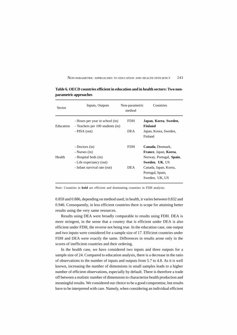
243NON-PARAMETRIC APPROACHES TO EDUCATION AND HEALTH EFFICIENCY
Table 6. OECD countries efficient in education and in health sectors: Two non-parametric approaches
Inputs, Outputs Non-parametric Countries
method
- Hours per year in school (in) FDH Japan, Korea, Sweden,Education - Teachers per 100 students (in) Finland
- PISA (out) DEA Japan, Korea, Sweden,
Finland
- Doctors (in) FDH Canada, Denmark,
- Nurses (in) France, Japan, Korea,
Health - Hospital beds (in) Norway, Portugal, Spain,
- Life expectancy (out) Sweden, UK , US
- Infant survival rate (out) DEA Canada, Japan, Korea,
Portugal, Spain,
Sweden, UK, US
Note: Countries in bold are efficient and dominating countries in FDH analysis.
0.859 and 0.886, depending on method used; in health, it varies between 0.832 and
0.946. Consequently, in less efficient countries there is scope for attaining better
results using the very same resources.
Results using DEA were broadly comparable to results using FDH. DEA is
more stringent, in the sense that a country that is efficient under DEA is alsoefficient under FDH, the reverse not being true. In the education case, one output
and two inputs were considered for a sample size of 17. Efficient countries under
FDH and DEA were exactly the same. Differences in results arose only in thescores of inefficient countries and their ordering.
In the health case, we have considered two inputs and three outputs for a
sample size of 24. Compared to education analysis, there is a decrease in the ratioof observations to the number of inputs and outputs from 5.7 to 4.8. As it is well
known, increasing the number of dimensions in small samples leads to a higher
number of efficient observations, especially by default. There is therefore a tradeoff between a realistic number of dimensions to characterize health production and
meaningful results. We considered our choice to be a good compromise, but results
have to be interpreted with care. Namely, when considering an individual efficient
Sector

244 JOURNAL OF APPLIED ECONOMICS
country, it is important to take into account if that country is an outlier, or if itefficient by default in FDH analysis. Interestingly enough, the use of DEA eliminated
an important number of FDH efficient by default observations.
Three countries appear as efficient no matter what method or sector is considered–Korea, Japan and Sweden. Japan is the best performer in education and one of
the best in health as far as outputs are concerned, and does not spend too many
resources. Korea is a very good education performer, and it spends very little onhealth with surprisingly good results in comparative terms. Sweden is never the
best performer in terms of the output indicators, although outcomes are always
clearly above the average. Efficient use of resources led this Nordic country tooutperform or dominate a good number of other countries in the sample, either in
education or health.
A comparison of Japan and Sweden leads to some interesting insights thatshow there are different ways of being efficient. In education, Japanese students
spend more time at school in classes that are a bit larger. In health, if Japan does
not have so many doctors per habitant, it exceeds in hospital beds.Measuring efficiency when one considers the financial resources allocated to
a sector is different from assessing efficiency from the measurement of resources
in physical terms, as in our models. Countries where resources are comparativelyexpensive could be wrongly considered as not efficient under an alternative
specification. Also, countries where resources considered (doctors, nurses, hospital
beds, and teachers) are comparatively cheaper would appear as efficient in financialterms.15
We evaluated efficiency across countries in two sectors, essentially comparing
resources to outputs. This opens the way to a different but related line of research,which is to explain why some countries are more efficient than others when it
comes to education or health provision. Different plausible linkages can be
investigated. We point out some, to suggest some future research. As an importantpart of education or health expenditure and provision is public, it could be the case
that inefficient provision is related to public sector inefficiency. Other differences
across countries can play a role in explaining our results. For example, a differentpopulation density or composition may well imply different needs from an input
perspective in order to attain the same measured outputs. Also, different levels of
GDP per head or of educational attainment by the adult population could imply
15 Results not presented here and available from the authors suggest this would be the case ofSweden, where costs are high, and of some Eastern European countries, where costs are low.

245NON-PARAMETRIC APPROACHES TO EDUCATION AND HEALTH EFFICIENCY
different outcomes in health or education, even under efficient public services.16
Countries are also different in what concerns the mix of public and private funding
of education and health (see Table 1). One possible source of inefficiency could
derive from the interaction between these.Clearly, and after measuring efficiency, identifying the (in)efficiency sources
would be of great importance in economic policy terms.
References
Afonso, António, Ludger Schuknecht, and Vito Tanzi (2004), “Public sectorefficiency: An international comparison”, Public Choice, forthcoming.
Barro, Robert J., and Jong-Wha Lee (2001), “Schooling quality in a cross-section
of countries”, Economica 68: 465-488.Bowlin, William (1998), “Measuring performance: An introduction to data
envelopment analysis (DEA)”, Journal of Cost Analysis Fall 1998: 3-27.
Charnes, Abraham, William W. Cooper, and Eduardo Rhodes (1978), “Measuringthe efficiency of decision making units”, European Journal of Operational
Research 2: 429–444.
Clements, Benedict (2002), “How efficient is education spending in Europe?”,European Review of Economics and Finance 1: 3-26.
Coelli, Tim, D. S. Prasada Rao, and George E. Battese (1998), An Introduction to
Efficiency and Productivity Analysis, Boston, Kluwer.De Borger, Bruno, and Kristian Kerstens (1996), “Cost efficiency of Belgian local
governments: A comparative analysis of FDH, DEA, and econometric
approaches”, Regional Science and Urban Economics 26: 145-170.Deprins, Dominique, Léopold Simar, and Henry Tulkens (1984), “Measuring labor-
efficiency in post offices”, in M. Marchand, P. Pestieau and H. Tulkens, eds.,
The Performance of Public Enterprises: Concepts and Measurement,
Amsterdam, North-Holland.
EC (2002), “Public finances in EMU, 2002”, European Economy 3/2002, European
Commission.Evans, David, Ajay Tandon, Christopher Murray, and Jeremy Lauer (2000), “The
comparative efficiency of national health systems in producing health: An
analysis of 191 countries”, GPE Discussion Paper Series 29, Geneva, WorldHealth Organisation.
16 Barro and Lee (2001), with different countries, data and time period, found a statisticallysignificant influence of these two variables on student achievement.
246 JOURNAL OF APPLIED ECONOMICS
Fakin, Barbara, and Alain de Crombrugghe (1997), “Fiscal adjustment in TransitionEconomies: Social transfers and the efficiency of public spending, a comparison
with OECD countries”, Policy Research Working Paper 1803, Washington,
World Bank.Farrell, Michael J. (1957), “The measurement of productive efficiency”, Journal of
the Royal Statistical Society, Series A 120: 253-290.
Ferrier, Gary D., and C. A. Knox Lovell (1990), “Measuring cost efficiency in banking:Econometric and linear programming evidence”, Journal of Econometrics 46:
229-245.
Gupta, Sanjeev, and Marijn Verhoeven (2001), “The efficiency of governmentexpenditure – experiences from Africa”, Journal of Policy Modelling 23: 433-
467.
Hanushek, Eric A., and Javier A. Luque (2002), “Efficiency and equity in schoolsaround the world”, Working Paper 8949, Cambridge, MA, NBER.
Jondrow, James, C. A. Knox Lovell, Ivan Materov, and Peter Schmidt (1982), “On
the estimation of technical inefficiency in the stochastic frontier productionfunction model”, Journal of Econometrics 19: 233-238.
OECD (2001), Knowledge and Skills for Life – First Results from Pisa 2000, Paris,
OECD.OECD (2002a), Education at a Glance – OECD Indicators 2002, Paris, OECD.
OECD (2002b), OECD Health Data 2002, Paris, OECD.
Sengupta, Jati (2000), Dynamic and Stochastic Efficiency Analysis – Economics
of Data Envelopment Analysis, Singapore, World Scientific.
Simar, Léopold and Paul Wilson (2003), Efficiency Analysis: The Statistical
Approach, lecture notes.St. Aubyn, Miguel (2002), “Evaluating efficiency in the Portuguese health and
education sectors”, unpublished manuscript, Lisbon, Banco de Portugal.
St. Aubyn, Miguel (2003), “Evaluating efficiency in the Portuguese educationsector”, Economia 26: 25-51.
Thanassoulis, Emmanuel (2001), Introduction to the Theory and Application of
Data Envelopment Analysis, Boston, Kluwer Academic Publishers.

247ESTIMATION WITH PRICE AND OUTPUT UNCERTAINTY
Journal of Applied Economics. Vol VIII, No. 2 (Nov 2005), 247-257
ESTIMATION WITH PRICE AND OUTPUT UNCERTAINTY
MOAWIA ALGHALITH *
St. Andrews University
Submitted September 2003; accepted November 2004
This paper extends the existing estimation methods to allow estimation under simultaneousprice and output uncertainty. In contrast with the previous literature, our approach isapplicable to the direct and indirect utility functions and does not require specification andestimation of the production function. We derive estimating equations for the two mostcommon forms of output risk (additive and multiplicative risks) and empirically determinewhich form is appropriate. Moreover, our estimation method can be utilized by futureempirical studies in several ways. First, our method can be extended to include multiplesources of uncertainty. Second, it is applicable to other specifications of output uncertainty.Third, it can be used to conduct hypothesis tests regarding the functional forms anddistributions. Furthermore, it enables the future empirical researcher to empirically verify/refute the theoretical comparative statics results.
JEL classification codes: D8, D2Key words: estimating equations, output uncertainty, price uncertainty, utility
I. Introduction
Empirical studies in the presence of hedging (usually agricultural commodities)
are abundant. They derive estimating equations under output price uncertainty by
applying uncertainty analogues of Hotelling’s lemma and Roy’s identity to theindirect expected utility function (see Pope 1980, and Dalal 1990). However, their
method is not directly applicable to the models with price and output uncertainty.
While focusing on hedging, few empirical studies include both price and outputuncertainty using a computational approach.
The literature can be divided into three main categories: Literature that deals
with theoretical estimating methods, empirical literature that includes hedging,and empirical literature in the absence of hedging.
∗ I am grateful to the referees and the co-editor Mariana Conte Grand for their helpful comments.Correspondence should be addressed to: [email protected].
JOURNAL OF APPLIED ECONOMICS248
The first category includes Pope (1980) and Dalal (1990). They used dualitytheory to derive estimating equations based on approximation of the indirect utility
function. These equations use the decision variable(s) as the dependent variable(s)
and the moments of the distribution as the independent variables.The second category focuses on hedging of agricultural commodities.
Arshanapalli and Gupta (1996) and Antonovitz and Roe (1986) derived estimating
equations under output price uncertainty by adopting duality theory; that is,applying uncertainty analogues of Hotelling’s lemma and Roy’s identity to the
indirect expected utility function (Pope and Dalal’s approach). Other studies did
not use duality theory. For example, Lapan and Moschini (1994) and Rolfo (1980)employed a computational approach. Rolfo computed the ratio of hedging to
expected output for cocoa producers. Lapan and Moschini calculated the same
ratio for soya bean farmers. Li and Vukina (1998) showed that dual hedging underprice and output uncertainty reduces the variance of the income of corn farmers.
The third category does not include hedging. Relying on duality theory,
Appelbaum and Ullah (1997) provided a non-parametric estimation of the momentsfor some manufacturing industries facing output price uncertainty. Here too, some
studies did not utilize duality theory. Chavas and Holt (1996) dealt with estimation
under technological uncertainty. They devised methods for generating data seriesfor the moments of the distributions. Relying on Taylor approximations of the
direct utility function, Kumbhakar (2002a, 2002b, and 2001) provided empirical
analysis using samples of Norwegian salmon farmers. Kumbhakar (2002a) assumedquadratic utility and production functions under output price uncertainty.
Kumbhakar (2002b and 2001) adopted Just and Pope’s specification of production
uncertainty. Kumbhakar (2002b) dealt with estimation under production risk andtechnical inefficiency. Kumbhakar (2001) included output price, input prices, and
production uncertainty.
There is a shortage of empirical studies under uncertainty in the absence ofhedging (especially studies that deal with output uncertainty). Kumbhakar (2002b
and 2001) provided empirical analysis under output uncertainty. Our approach
differs from Kumbhakar’s approach in three respects. First, Kumbhakar relied onthe direct utility function, whereas we use a combination of the direct and indirect
utility functions; that is, we modify the duality approach to accommodate output
uncertainty. Second, Kumbhakar adopted a different specification of outputuncertainty. Third, our approach does not require specification or estimation of
the production function.
Consequently, this paper provides three main contributions. First, it extends

249ESTIMATION WITH PRICE AND OUTPUT UNCERTAINTY
existing estimation methods to allow empirical estimation under simultaneous priceand output uncertainty. Second, it derives estimating equations for the most twocommon forms of output risk: additive risk and multiplicative risk (see Honda 1987,Grant 1985, Lapan and Moschini 1994). Third, it empirically determines which formis appropriate. When modeling output uncertainty, the multiplicative specificationis consistently chosen over the additive form, despite the latter being arguablyintuitively more obvious. The rationale for this seems to be that when productionrisk is the only source of uncertainty, additive uncertainty does not reduce outputbelow the certainty level, while multiplicative uncertainty does. We empiricallyshow this need not be always the case and thus additive uncertainty is indeed areasonable a priori method of modeling production uncertainty.
II. Additive output uncertainty
A competitive firm (sector) faces an uncertain output price given by p= ,σε+p
where ε is random with E [ε] = 0 and Var(ε) = 1, so that E [p] = p and Var (p) = σ 2.The level of output realized at the end of the production process is not known exante. Output has both a random and a nonrandom component and is given by q,where q is random and defined as q= y + θη (additive risk), where η is random withE[η] = 0 and Var (η) = 1, so that Var (q) = θ 2 and the expected value of output isE(q) = y. Both σ and θ are shift parameters with initial values equal to 1. We assumethat ε and η are statistically independent and thus Cov (ε, η) = 0.1 Costs are knownwith certainty and are given by a cost function, c(y,w), which displays positive andincreasing marginal costs so that c
y(y,w) > 0 and c
yy (y,w) > 0. While y represents
expected output, it may usefully be thought of as the level of output, which wouldprevail in the absence of any random shocks to output. The firm may be thought ofas having its target level of output and committing inputs that would generate thislevel in the absence of any random shocks. The cost function is then the minimumcost of producing any arbitrary output level y given the input price vector w. Thus,profit is ).,( wycpq−=π The firm is risk-averse and seeks to maximize the expected
utility of the profit. It therefore seeks to solve the problem
The maximization problem implies the existence of an indirect expected utility
function V, such that
1 This assumption is empirically verified in Section IV.
))].,(([)]([max wycpqUEUEy
−=π

JOURNAL OF APPLIED ECONOMICS250
where y* is the optimal value of y. Let π* represent the value of π correspondingto y*. The envelope theorem applied to (1) implies
Consider the following approximation
multiplying through by ε and taking expectations of both sides,
Similarly,
Now, since π is a constant, )ˆ('' πU is a parameter which can be estimated.Letting ),ˆ('' πβ U≡ and substituting the approximations for ]*)('[ επUE
and ]*)('[ εηπUE into (2) we obtain
In order to get an expression for Vσ we need to have an expression for).,,,( wpV θσ Since the form of the indirect expected utility function is not known,
we approximate it by a second-order Taylor series expansion about the arbitrary
point )ˆ,ˆ,ˆ,ˆ( wpA θσ (for a detailed approximation, see Satyanarayan 1999 andArshanapalli and Gupta 1996). Letting subscripts denote partial derivatives, we
obtain
where tildes denote deviations from the point of expansion and all the partial
),,,( wpV θσ ))]*,()*(([ wycypUE −+= θη (1)
].*)('[]*)('[* ηεπθεπσ σ UEUEyVV +=≡
∂∂
(2)
).ˆ*)(ˆ('')ˆ('*)(' πππππ −+≈ UUU
=−+≈ ][ˆ]*[)ˆ(''][)ˆ(']*)('[ επεππεπεπ EEUEUUE
.)ˆ(''*])**[()ˆ('' σπεσεθησεθηπ UycypypEU =−+++= (3)
≈]*)('[ εηπUE .)ˆ('']*[)ˆ('' σθπεηππ UEU = (4)
.22* θβσ
σ −=V
y (5)
,~~~~)( θσ σθσσσσσσ VVwVpVAVV
iiip ++++≈ ∑ (6)
]*[)ˆ('' εππ EU
251ESTIMATION WITH PRICE AND OUTPUT UNCERTAINTY
derivatives on the right-hand side of (6) are evaluated at the point of expansion.Substituting (6) into (5) yields
The parameters (to be estimated) are σθσσσσσ VVVVAV ip ,,,),( and β. Note
that y*2 is homogeneous of degree 0 in all the parameters, and thus we need somenormalization.2 The established procedure in the literature is to set β equal to -1
(see Appelbaum et al. 1997 and Dalal 1990).3
Hence, our final estimating form is
III. Multiplicative output uncertainty
In this section we derive an estimating equation for the multiplicative output
uncertainty model. If output risk is multiplicative, q = v y, where v = 1+ θη and thus
E[v] = 1.This estimating equation will be comparable to the additive uncertaintyequation. The objective function is
and as before, the maximization problem implies the existence of an indirect utility
function V such that
The envelope theorem applied to (9) implies
.
~~~~)(22* θ
βσ
θσ σθσσσσσ
−++++
=∑ VVwVpVAV
y iiip
(7)
2 It is homogeneous of degree 0 because, for instance, doubling the values of all the parameterswill have no impact on the value of y*. Thus normalization is needed to make y* sensitive tothe proportional change in the value of all the parameters.
3 Note that we used -1 rather than 1 because β denotes U’’ ( π), which must be negative (by theconcavity of the utility function).
.
~~~~)(22* θ
σ
θσ σθσσσσσ
−++++
−=∑ VVwVpVAV
y iiip
(8)
))],,(([max wycpvyUEy
−
),,,( wpV θσ ))]*,(*([ wycpvyUE −= (9)
^
,

JOURNAL OF APPLIED ECONOMICS252
We need to approximate επ*)('[UE and ].*)('[ ηεπUE Proceeding as before,
where β is defined as before. Similarly,
Substituting (11) and (12) into (10) and rearranging, we obtain
Using (6), yields
where all the partial derivatives are evaluated at the point of expansion. Onceagain, y* is homogeneous of degree 0 in all the parameters and thus normalization
is required. As before we normalize β equal to -1 so that the estimating equation is
IV. Empirical exercise
The data required for estimation of (8) and (15) include the mean and standard
deviation of output and its price. Since these are not directly observable, we have
to generate these values from observable data. There is some arbitrariness in themethod chosen to do so, since there is no unambiguously “best” approach. Some
empirical studies have adopted an extremely simple approach, such as Arshanapalli
and Gupta (1996), who used a simple moving average process, while others usemuch more complex methods.
].*)('[*]*)('[*]*)('[* ηεπθεπεπσ UEyuEyvUEyV +== (10)
]*)('[ επUE ,**)ˆ('' σβσπ yyU ≡≈ (11)
]*)('[ ηεπUE .**)ˆ('' σθβσθπ yyU ≡≈ (12)
.)1( 2
2*
θβσσ
+= V
y (13)
,)1(
~~~~)(
22*
θβσ
θσ σθσσσσσ
+
++++=
∑ VVwVpVAV
y iiip
(14)
.)1(
~~~~)(
22*
θσ
θσ σθσσσσσ
+
++++−=
∑ VVwVpVAV
y iiip
(15)

253ESTIMATION WITH PRICE AND OUTPUT UNCERTAINTY
In order to generate a series of expected prices, we have chosen to use themethod developed by Chavas and Holt (1996), where the price at time t is considered
as a random walk with a drift. Thus,
where pt is the price al time t, p
t-1 is the previous year’s market price, δ is a drift
parameter, and εi is a random variable with E[ε
i] = 0. Hence
.][ 1−+= tt ppE αδ
Similarly, to generate a series for y*, we model output at time t by
where qt is the output at time t, q
t-1 is the previous year’s output, and u
i is an error
term with E[ui] = 0. Hence,
To generate series for σ we will also use Chavas and Holt’s method:
where the weights are 0.5, 0.33, and 0.17 (the same weights used by Chavas and
Holt). This is done to reflect the idea of declining weights. The price variance isthus measured as the weighted sum of squared deviations of the previous prices
from their expected values.
Similarly, the variance of output is
We can implement our estimating methods using manufacturing data;
uncertainty in the manufacturing sector is as common as it is in the agriculturalsector.
Natural catastrophes, strikes, legal suits and blackouts are some sources of
,1 itt pp εαδ ++= −
,1 itt uqq ++= −ϕφ
.*][ 1−+== ttt qyqE ϕφ
,)( 23
1
2jtjtjt
jjt pEpw −−−
=
−= ∑σ
.)*( 23
1
2jt
jjtjt yqw −
=− −= ∑θ

JOURNAL OF APPLIED ECONOMICS254
uncertainty in the manufacturing sector. Demand shocks are the main cause of
price uncertainty. For example, Appelbaum and Ullah (1997) identified output price
uncertainty in several manufacturing industries. We used U.S. manufacturing time
series data. The manufacturing output (q) is produced using four inputs: materials
(m), energy (e), capital (k), and labor (l), with prices given, respectively, by wm, w
e,
wk, and w
l. Gross output price and quantity data are taken directly from the
worksheets of the U.S. Department of Commerce, Bureau of Economic Analysis.
The quantity and the price of each input are derived or taken from Department of
Census, Bureau of Economic Analysis.
Rewriting the estimating equations to explicitly introduce the four input prices
we will be using, (8) becomes
and equation (15) becomes
For all the equations, the point of expansion is the mid-point in the data series.
First, we generated data series for ε and η using Chavas and Holt’s method to
test the independence assumption, using a standard test that relies on the correlation
factor and the t-ratio. We strongly (at 1% significance level) accepted the null
hypothesis that ε and η are independent. We used nonlinear least square
regressions to estimate our estimating equations. We estimated (16) and (17).
V. Results and conclusions
The results are reported in Table 1. While the additive uncertainty model has
an excellent fit, with F = 21.99 and α (the probability that all the parameters equal
zero) tends to 0; this is not the case for the multiplicative uncertainty model. The
latter has a very poor fit, where F = .71 and α = .664. Hence, we reject the model
altogether and conclude that the data is more consistent with the additive output
uncertainty model.
~~~~~~~)(2*
σθσ σθσσσσσσσσ +++++++
−=VVwVwVwVwVpVAV
ykkmmlleep (16)
,2θ−
.)1(
~~~~~~~)(2
22*
θσ
θσ σθσσσσσσσσ
+
+++++++−=
VVwVwVwVwVpVAVy kkmmlleep (17)
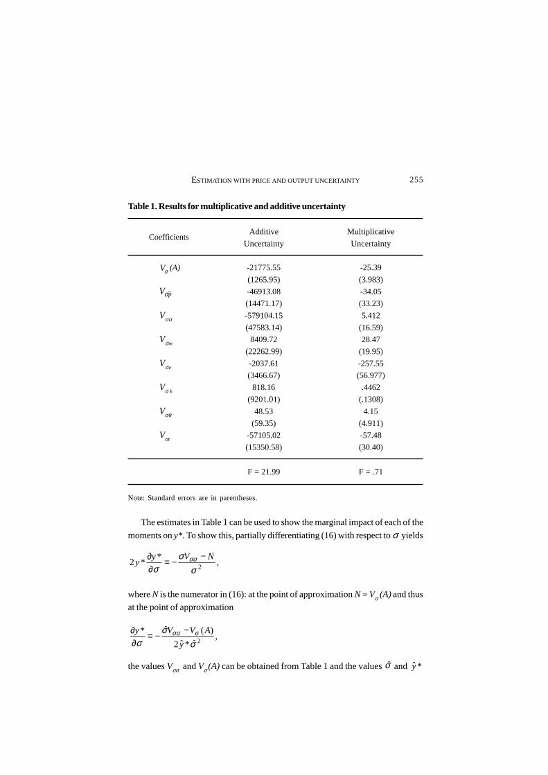
255ESTIMATION WITH PRICE AND OUTPUT UNCERTAINTY
Table 1. Results for multiplicative and additive uncertainty
Additive Multiplicative
Uncertainty Uncertainty
Vσ (A) -21775.55 -25.39
(1265.95) (3.983)
-46913.08 -34.05
(14471.17) (33.23)
Vσσ -579104.15 5.412
(47583.14) (16.59)
Vσm8409.72 28.47
(22262.99) (19.95)
Vσe-2037.61 -257.55
(3466.67) (56.977)
Vσ k 818.16 .4462
(9201.01) (.1308)
Vσθ 48.53 4.15
(59.35) (4.911)
Vσt-57105.02 -57.48
(15350.58) (30.40)
F = 21.99 F = .71
Note: Standard errors are in parentheses.
The estimates in Table 1 can be used to show the marginal impact of each of the
moments on y*. To show this, partially differentiating (16) with respect to σ yields
where N is the numerator in (16): at the point of approximation N = Vσ (A) and thus
at the point of approximation
,ˆ*ˆ2
)(ˆ*2σ
σσ
σσσ
y
AVVy −−=∂∂
the values Vσσ and Vσ (A) can be obtained from Table 1 and the values σ and *y
,*
*22σ
σσ
σσ NVyy
−−=∂∂
Coefficients
pVσ
Vσ

JOURNAL OF APPLIED ECONOMICS256
are known values in the data series. Hence the value σ∂
∂ *ycan be obtained.
Similarly,
An increase in σ and θ means an increase in price riskiness and output riskiness,
respectively. We found < 0, θ∂∂ *y
< 0 and p
y
∂∂ *
> 0. Thus, an increase in price
(output) riskiness reduces optimal output. The increase in the price mean increases
optimal output. These results are intuitive and consistent with the theory.
To conclude, in at least this instance it appears that additive output uncertainty
might be the more appropriate method of modeling output uncertainty. But this
does not imply that, in general, multiplicative risk should be ruled out. Since some
microeconomic theorists prefer the multiplicative form, the results are illustrative
that additive risk shouldn’t be ruled out without empirical evidence.
References
Antonovitz, Frances and Terry Roe (1986), “A theoretical and empirical approach
to the value of information in risky markets”, Review of Economics and Statistics
68: 105-114.
Appelbaum, Eli and Aman Ullah (1997), “Estimation of moments and production
decisions under uncertainty”, Review of Economics and Statistics 79: 631-
637.
Arshanapalli, Bala and Omprakash Gupta, (1996), “Optimal hedging under output
price uncertainty”, European Journal of Operational Research 95: 522-36.
Chavas, Jean-Paul and Matt Holt, (1996), “Economic behavior under uncertainty:
A joint analysis of risk and technology”, Review of Economics and Statistics
51: 329-335.
Dalal, Ardeshir (1990), “Symmetry restrictions in the analysis of the competitive
firm under price uncertainty”, International Economic Review 31: 207-11.
Grant, Dwight (1985), “Theory of the firm with joint price and output risk and a
forward market”, American Journal of Agricultural Economics 67: 60-635.
,ˆ2ˆ*ˆ2
1*
−−=
∂∂ θ
σθσθV
y
y
.ˆ*ˆ2
*
σσ
y
V
p
y p−=∂
∂
σ∂∂ *y

257ESTIMATION WITH PRICE AND OUTPUT UNCERTAINTY
Honda, Yuzo (1983), “Production uncertainty and the input decision of thecompetitive firm facing the futures market”, Economics Letters 11: 87-92.
Kumbhakar, Subal (2001), “Risk preferences under price uncertainties and
production risk”, Communications in Statistics: Theory and Methods 30: 1715-1735.
Kumbhakar, Subal (2002a), “Risk preference and productivity measurement under
output price uncertainty”, Empirical Economics 7: 461-472.Kumbhakar, Subal (2002b), “Specification and estimation of production risk, risk
preferences and technical efficiency”, American Journal of Agricultural
Economics 84: 8-22.Lapan, Harvey and Giancarlo Moschini (1994), “Futures hedging under price, basis,
and production risk”, American Journal of Agricultural Economics 76: 456-
477.Li, Dong-Feng and Tom Vukina (1998), “Effectiveness of dual hedging with price
and yield futures”’, Journal of Futures Markets 18: 541-561.
Pope, Rulon Dean (1980), “The generalized envelope theorem and priceuncertainty”, International Economic Review 21: 75-86.
Rolfo, Jaques (1980), “Optimal hedging under price and quantity uncertainty. The
case of cocoa producers”, Journal of Political Economy 88: 100-116.Setyanarayan, Sudhakar (1999), “Econometric tests of firm decision making under
dual sources of uncertainty” Journal of Economics and Business 51: 315-325.

259 RECYCLING OF ECO-TAXES, LABOR MARKET EFFECTS
Journal of Applied Economics. Vol VIII, No. 2 (Nov 2005), 259-278
RECYCLING OF ECO-TAXES, LABOR MARKET EFFECTSAND THE TRUE COST OF LABOR– A CGE ANALYSIS
K LAUS CONRAD* AND ANDREAS LÖSCHEL
Mannheim University and Centre for European Economic Research (ZEW)
Submitted May 2003; accepted May 2004
Computable general equilibrium (CGE) modeling has provided a number of importantinsights about the interplay between environmental tax policy and the pre-existing taxsystem. In this paper, we emphasize that a labor market policy of recycling tax revenuesfrom an environmental tax to lower employers’ non-wage labor cost depends on how thecosts of labor are modeled. We propose an approach, which combines neoclassicalsubstitutability and fixed factor proportions. Our concept implies a user cost of laborwhich consists of the market price of labor plus the costs of inputs associated with theemployment of a worker. We present simulation results based on a CO
2 tax and the recycling
of its revenues to reduce the non-wage labor cost. One simulation is based on the marketprice of labor and the other on the user cost of labor. We found a double dividend under thefirst approach but not under the second one.
JEL classification codes: D58, J30, Q25Key words: market-based environmental policy, carbon taxes, double dividend, computablegeneral equilibrium modeling
I. Introduction
Computable general equilibrium (CGE) analyses have played over the last ten
years a key role in the evaluation of green tax reforms, the reorientation of the taxsystem to concentrate taxes more on “bads” like pollution and less on “goods”
like labor input or capital formation. The ongoing concern about the magnitude of
distortionary taxation suggests the possibility of using environmental taxes toreplace existing factor and commodity taxes. A conjecture called the “double
* Klaus Conrad (corresponding author): Mannheim University, Department of Economics, L7,3-5, D-68131 Mannheim, Phone: +49 621 181 1896, Fax: +49 621 181 1893, e-mail:[email protected]. We are grateful to two anonymous referees for their helpfulcomments. Andreas Löschel acknowledges financial support from the DeutscheForschungsgemeinschaft (DFG), Graduiertenkolleg Umwelt- und Ressourcenökonomik.

JOURNAL OF APPLIED ECONOMICS260
dividend hypothesis” points out that environmental taxes have two benefits: theydiscourage environmental degradation and they raise revenue that could offsetother distortionary taxes.1 The non-environmental dividend can be defined invarious ways. Given the important unemployment problem in the EU, priority hasbeen given to the analysis of distortions in the labor market that might explainpersisting unemployment.2 The revenue from the pollution taxes is recycled to cutlabor taxes. On the one side, the narrow base of an energy tax constitutes aninherent efficiency handicap. On the other side, the impact of the tax reform on pre-existing inefficiencies in taxing labor could offset this handicap and a doubledividend arises. Therefore, in principle a double dividend can arise only if (i) thepre-existing tax system is significantly inefficient on non-environmental groundsand (ii) the revenue-neutral reform significantly reduces this prior inefficiency. Thedouble dividend actually arises only if the second condition operates with sufficientforce. However, it could also arise if the burden of the environmental tax fallsmainly on the undertaxed factor (e.g., immobile capital) and relieves the burden ofthe overtaxed factor (i.e., labor).3 Since no existing tax systems are likely in asecond-best optimum, i.e., minimizing the sum of deadweight losses given a fixedbudget, the scope for a double dividend is always present.
Although CGE modeling has provided a number of important insights aboutthe interplay between environmental tax policy and the pre-existing tax system,much remains to be done to improve our understanding of market-basedenvironmental policy. One reason is that some CGE modelers affirm the doubledividend hypothesis while others could not find a double dividend outcome. Thespecification of the labor market, for instance, could be crucial to the discussionon the effect of environmental policy on employment. A labor market policy ofrecycling tax revenues from an environmental tax to lower employers’ non-wagelabor cost depends on how the labor market is modeled. The objective of ouranalysis is not to show that non-competitive labor markets could provide a potentialchannel for a double dividend outcome. A variety of approaches are discussed inthe literature to analyze the impacts of an ecological tax reform in the presence of
wage setting institutions and involuntary unemployment. Typically, labor market
1 For a state of the art review on the double dividend issue, see Goulder (1997) and Bovenbergand Goulder (2001).
2 For theoretical papers on the double dividend issue, see Goulder (1995) and Bovenberg andGoulder (1996). See Jorgenson and Wilcoxen (1992), Proost and van Regemorter (1995) andWelsch (1996) for empirical papers.
3 See Bovenberg and Goulder (2001) on this point.

261 RECYCLING OF ECO-TAXES, LABOR MARKET EFFECTS
imperfections are introduced by an upward sloping wage setting curve, whichreplaces the labor supply curve used in the competitive model. The equilibriumwage and employment level are now determined by the intersection of the wagesetting and the labor demand curve. The theory of equilibrium unemploymentoffers three microeconomic models, which all capture specific institutional factorsof actually existing labor markets – namely trade union models, efficiency wagemodels, and mismatch models. Each model is appropriate to describe a specificpart of the multi-facetted phenomenon of involuntary unemployment. So, unlikethe recent double dividend literature, we will not emphasize the empirical relevanceof a certain labor market model, but our aim is instead to attack the way the costsof labor are conceived in all neoclassical models.
The objective of this paper therefore is to advocate an approach where thecost of labor is not just wage per day, but the cost of the working place per day,including the wage. This new concept is that of the “user cost of labor”, for which,the cost of an additional worker includes not just salary, but also the costs ofinputs tied to the worker (e.g., office equipment, electricity, material, etc.).
Such a view will have a reduced impact on substitution possibilities betweenlabor and other inputs and hence will affect the outcome of a double dividendpolicy in a different way than under the traditional approach of pure market prices.We will use an approach proposed by Conrad (1983) who combines the approachesto neoclassical substitutability and fixed factor proportions. This cost-priceapproach uses Leontief partially fixed factor proportions to identify both adisposable or variable part and a bound or fixed portion of each input. The truecost, or cost price, of any input consists of its own price plus the costs associatedwith the portion of that input bound to other inputs. Within the cost-price framework,the demand for an input can be separated into a committed component linked tothe use of other inputs, and a disposable component that is free for substitution.At one extreme, when the disposable quantities of all inputs equal zero, no factorsubstitution is possible and the cost-price approach reduces to the Leontief fixed-proportion case. At the other extreme, when the committed quantities of all inputsare zero, the neoclassical model is relevant and the cost-price of any input equatesthe market price.
We include this user-cost approach in CGE modeling and then run a model tocheck its relevance and to understand the effects of imperfect substitution in thelabor market.4 We econometrically estimate cost share equations in cost-prices
4 In Section V we relate our result to the findings in the theoretical and empirical literature onthe double dividend issues.

JOURNAL OF APPLIED ECONOMICS262
and then use cost prices as well as market prices to investigate the double dividendhypothesis.
The paper is organized as follows. In Section II, we present the cost-price
approach and in Section III the parameter estimates for a restricted version of themanufacturing industry. In Section IV, we briefly outline our CGE model. In Section
V, we present our simulation results based on a CO2 tax and the recycling of its
revenues to reduce the non-wage labor cost. One simulation will be based onmarket prices and the other one on cost prices. Our objective is to compare the
results in the light of the conjecture of a double dividend. The conclusion from our
result is summarized in Section VI.
II. Conditioned input demand and cost share equations in cost-prices
In contrast to Leontief production functions, we assume that only fractions of
the input quantities are related to each other in fixed factor proportions and that
therefore, in contrast to the neoclassical theory, only fractions of the input quantitiesare disposable for substitutions. With capital, labor and energy as inputs, we
regard a truck, a truck driver and the minimal possible fuel consumption as bound
inputs. In general, however, not the total quantity of an input is bound by otherinputs with fixed proportions, but a fraction is unbound and disposable for
substitution. It is this fraction which is relevant for a reallocation of inputs if
relative factor prices change. If the energy price increases, the maintenance of themachinery will be improved (an additional worker), and truck drivers will drive
slower (working overtime or less mileage per day). However, this substitution
effect can primarily be observed with respect to the unbound component of aninput. Bound factors like machinery, the stock of trucks, or truck drivers are not
objects of a substitution decision; they will be replaced either simultaneously or
not at all as one more unit is linked to high costs due to bound inputs (an additionaltruck requires an additional truck driver). In case of a higher energy price, therefore,
the disposable energy input will be the one that will be reduced. The fact that other
inputs are bound to energy should be indicated by a cost-price or user cost inwhich the price of energy enters with an appropriate weight. In order to take into
account this aspect, we separate the quantity of an input (vi) into a bound part and
into an unbound one:5
5 For more details, see Conrad (1983).

263 RECYCLING OF ECO-TAXES, LABOR MARKET EFFECTS
where iv is the number of units of factor i bound by the usage of the remaining
n - 1 inputs, and iv is the disposable quantity of factor i. The bound quantity of aninput, ,iv depends with fixed factor proportions upon the disposable quantities of
the other inputs. Here, iv is a simple sum, defined as
where αij is the quantity of v
i bound to one disposable unit of v
j . Substituting (2)
into (1) yields
where αii = 1
by definition. If the disposable part of input j is increased by one unit, this increases
the total quantity of input j by just this unit and all other inputs i (i = 1,..., n, i ≠ j)by the quantities α
ij. These α
ij coefficients constitute a matrix A = (α
ij) that describes
the degree of affiliation for any data set. If αij = 0 (i ≠ j) for all i and j, the
neoclassical model is relevant and the cost-price of any input is its own price. If
iv = 0 (or vi = )iv for all i, no factor substitution is possible and the cost price
approach reduces to the Leontief fixed proportion production function.
We next replace the quantities vi in the cost minimizing approach by the
partitioning given in (3). Instead of
where x is the given output quantity and Pi is the price for i, we write
where
and αjj = 1, j = 1,…n
is the cost-price of input j. It consists of its own price (Pj) plus the additional costs
,ˆiii vvv += ni ...,1= (1)
∑≠
=ij
jiji vv ,ˆα ,0≥ijα ,,...1 ni = (2)
,ˆ1
∑=
=n
jjiji vv α (3)
,),...,(|min 1
=∑i
nii vvHxvP (4)
=∑j
njj vvFxvP )ˆ,...,ˆ(|ˆˆmin 1 (5)
∑=j
jijj PP αˆ (6)

JOURNAL OF APPLIED ECONOMICS264
associated with factors bound to vj. By substituting the cost-minimizing factor
demand functions )ˆ,...,ˆ;(ˆ 1 njj PPxfv = into (3) we obtain the cost-minimizing input
quantities in terms of cost prices 1P ,... .ˆnP The dual cost function with respect to
the cost prices is then:
The analogue to Shephard’s lemma holds:
Equations (8) and (9) provide the disposable amounts of each input as well asthe cost minimizing quantities of total inputs. From Equation (9), we can determine
the cost shares (wi) of each factor as follows:
These share equations can then be used to empirically estimate the parameters
of the cost prices.6 In the next Section, we will estimate econometrically the cost-
price model.7
III. Empirical results for a Cobb-Douglas cost function
As a specification of the cost function we will choose the simplest case,
namely a cost function of the Cobb-Douglas type (henceforth, CD). However, an
).ˆ,...,ˆ;(.ˆ)ˆ,...,ˆ;( 11 njj
jn PPxfPPPxC ∑= (7)
ii
vP
PxCˆ
ˆ)ˆ;( =
∂∂ (8)
∑∑ ==
∂∂
∂∂=
∂∂
jiiij
j i
j
ji
vvP
P
P
C
P
PxCˆ.
ˆ
ˆ)ˆ;( α (9)
( ).
ˆ;ln.
∂
∂==i
iii
i P
PxCP
C
vPw (10)
6 Technical change can be introduced into the cost prices (see Olson and Shieh 1989). We haveomitted this aspect in our CGE analysis.
7 The cost-price concept has been employed econometrically within a model of consumerbehaviour by Conrad and Schröder (1991). They use a specification of an expenditure functionin durables and non-durables and identify the part of goods complementary to consumer

265 RECYCLING OF ECO-TAXES, LABOR MARKET EFFECTS
durables like gasoline, electricity or repair services. In the GEM-E3 model for the EU (Caproset al. 1996) the demand for durables takes into account the demand for complementary goodsbound to consumer durables.
8 We are indebted to Henrike Koschel and Martin Falk for providing us with the data set. Formore details see Koschel (2001) and Koebel et al. (2003).
approach with cost prices and committed inputs does not result in simplemeasures of the degree of substitutability as in the conventional CD case where
the elasticity of substitution is unity and all inputs are price substitutes. As shown
in Conrad (1983), even under the CD-assumption, variable elasticities ofsubstitution and complementary relations are possible. Under our assumption of
constant returns to scale and disembodied factor augmenting technical change,
bj.t, the CD-cost function is ,ˆln).(ln)ˆ;(ln 0 j
jjj PtbxPxC ∑ +++= γα where
∑ =j
j 1γ and .0=∑j
jb Because of (10),
where .ˆ ∑≠
+=jk
kkjjj PPP α
We have nested the inputs of a sector, based on an input-output table with 49
sectors, such that in the first stage the inputs for the CD-production function are
capital K, labor L, electricity E, material M, and fossil fuel F. As data for disaggregatedenergy inputs are available only for a short period of time (1978-90), we are
constrained to a pooled time-series cross-section approach.8 A total of 49 sectors
for which data are available in the German national account statistics are pooledinto four sector aggregates: the energy supply sectors aggregate; the energy-
intensive manufacturing sectors aggregate; the non-energy-intensive
manufacturing sectors aggregate; the service sectors aggregate.The five-equation system, consisting of the five cost-share equations for K, L,
E, M, F, is estimated for each of the four sector aggregates, employing the panel
data set in yearly prices and cost shares. It is assumed that the cost prices areidentical in each sector aggregate (i.e., sectoral dummy variables are added only to
the coefficients γi in (11)).
Due to the high degree of non-linearity inherent in the share equations, we
+= ∑
jij
j
jjii
P
tbPw α
γˆ
.(11)
JOURNAL OF APPLIED ECONOMICS266
have simplified our approach by concentrating on the cost-price of labor. Hence,the composition (3) is reduced to
where i = 1, 2, 3, 4 for the four sector aggregates. The cost-prices for K, E, F,
M are therefore market prices, i.e. ,ˆ,, iKiK PP = ,ˆ
,, iEiE PP = iMiM PP ,,ˆ = and
.ˆ,, iFiF PP = The cost-price of labor is:
As mentioned before, αiL, i = K, E, M, F are the same for each sector aggregate
and so are the technical progress parameters bi, i = K, L, E, M, F. The system of
cost share equations we have to estimate is:
,ˆ
)...(.
.
,
,,,
iL
iMLiLMLMiM
i
iiMiM
P
Ptbtb
C
MPw
+++==
γαγ
.ˆ
)...(.
.
,
,,,
iL
iFLiLFLFiF
i
iiFiF
P
Ptbtb
C
FPw
+++==
γαγ
with LP as given in (13). In addition to using nonlinear techniques, the cost price
model must be estimated with non-negativity constraints imposed on the parameters
αiL, i = K, E, M, F. Table 1 presents the estimated parameters.The bias of technical change is capital, electricity and material using (b
k > 0,
bE > 0, b
M > 0), and labor and fossil fuel saving (b
L < 0, b
F < 0). The cost price of
labor (13) for the industry with the dummy variable of zero is
,ˆˆ. iiKLi KLK += α ,ˆii LL = ,ˆˆ. iiELi ELE += α ,ˆˆ. iiMLi MLM += α
iiFLi FLF ˆˆ. += α
(12)
iMMLiFFLiEELiKKLiLiL PPPPPP ,,,,,, ....ˆ αααα ++++= (13)
,ˆ
)..(.
,
,,,
iL
iLLiL
i
iiLiL
P
Ptb
C
LPw
+==
γ(14)
,ˆ
)...(.
.
,
,,,
iL
iKLiLKLKiK
i
iiKiK
P
Ptbtb
C
KPw
+++==
γαγ (15)
,ˆ
)...(.
.
,
,,,
iL
iELLiELEEi
i
iiEiE
P
Ptbtb
C
EPw
+++==
γαγ (16)
(17)
(18)

267 RECYCLING OF ECO-TAXES, LABOR MARKET EFFECTS
Table 1. Maximum likelihood estimates for parameters of cost-prices and technicalchange
Dummy for factors Parameters of technical progress Parameters of costs prices
γK
0.092 (17.173) bK
8.5 10-4 (0,935) αKL
0.002 (0,431)
γL
0.458 (11.340) bL
-0.005 (-1,824) αEL
0.055 (2,611)
γE
4·10-8 (6·10-6) bE
4.2 10-4 (1,889) αFL
0.072 (2,993)
γF
0.048 (3.508) bF
-0.002 (-1,143) αML
0.422 (3,128)
γM
* 0.402 –––– bM* 0.006 ––––
Log Likelihood = 3540.189, Observations: 637
Notes: Asymptotic t-ratios in parentheses. *As the error terms add to zero, they are stochasticallydependent and we have omitted equation (17) for estimation.
Using the αiL parameter estimates in Table 1, we conclude from (12) that an
additional unit of labor needs 0.002 units of capital, 0.055 units of electricity, 0.422
units of material and 0.072 units of fossil fuel. In other words, reducing labor input
by one unit will release 0.002 units of capital, 0.055 units of electricity, 0.422 unitsof material and 0.072 units of fossil fuel for possibilities of substitution as the
disposable components FMEK ˆ,ˆ,ˆ,ˆ increase with the reduction of L ).ˆ( L= In the
next Section we will use committed inputs, disposable inputs, and the correspondingcost-price of labor within the framework of a CGE model to investigate their impact
on the outcome of the double dividend conjecture.
IV. The features of the CGE model
This Section presents the main characteristics of a comparative-static multi-sector model for the German economy designed for the medium-run economic
analysis of carbon abatement constraints. Here, the concrete specification of the
model covers seven sectors and two primary factors.9 The choice of productionsectors captures key dimensions in the analysis of greenhouse gas abatement, such
..072.0422.0.055.0.002.0ˆFMEKLL PPPPPP ++++= (19)
9 The overall sectors are still the sectors F, E, M and the primary factors K and L. However, Fand M will be disaggregated to F
i and M
i, i = 1,2,3 (see Table 2).

JOURNAL OF APPLIED ECONOMICS268
as differences in carbon intensities and the scope for substitutability across energygoods and carbon-intensive non-energy goods. The energy goods identified in themodel are coal (COL), natural gas (GAS), crude oil (CRU), refined oil products (OIL)and electricity (ELE). Non-energy production consists of an aggregate energy-intensive sector (EIS) and the rest of production (OTH). Primary factors includelabor and capital, which are both assumed to be intersectorally mobile. Table 2summarizes the sectors and primary factors incorporated in the model.
Table 2. Overview of sectors and factors
Sectors Primary factors
1 COL Coal CAP Capital - K
2 OIL Refined oil products LAB Labor - L
3 GAS Natural gas4 ELE Electricity - E
5 CRU Crude oil
6 EIS Energy-intensive sectors7 OTH Rest of industry
-F
-M
The model is a well-known Arrow-Debreu model that concerns the interactionof consumers and producers in markets. Market demands are the sum of final andintermediate demands. Final demand for goods and services is derived from theutility maximization of a representative household subject to a budget constraint.In our comparative-static framework, overall investment demand is fixed at thereference level. The consumer is endowed with the supply of the primary factors ofproduction (labor and capital) and tax revenues (including CO
2 taxes). Household
preferences are characterized by an aggregate, hierarchical (nested) constantelasticity of substitution (CES) utility function. It is given as a CES composite of anenergy aggregate and a non-energy consumption composite. Substitution patternswithin the energy aggregate and the non-energy consumption bundle are reflectedvia Cobb-Douglas functions. Producers choose input and output quantities inorder to maximize profits. The structure in production is nested. At the top level,we have the KLEMF-structure with the CD specification in cost-prices. At thesecond level, a CES function describes the substitution possibilities between thematerial components. The primary energy composite is defined as a CES functionof coal, oil and natural gas. Key substitution elasticities are given in the Appendix.

269 RECYCLING OF ECO-TAXES, LABOR MARKET EFFECTS
The government distributes transfers and provides a public good (includingpublic investment) which is produced with commodities purchased at market prices.In order to capture the implications of an environmental tax reform on the efficiencyof public fund raising, the model incorporates the main features of the German taxsystem: income taxes including social insurance contributions, capital taxes(corporate and trade taxes), value-added taxes, and other indirect taxes (e.g. mineraloil tax).
All commodities are traded internationally. We adopt the Armington (1969)assumption that goods produced in different regions are qualitatively distinct forall commodities. There is imperfect transformability (between exports and domesticsales of domestic output) and imperfect substitutability (between imports anddomestically sold domestic output). On the output side, two types of differentiatedgoods are produced as joint products for sale in the domestic markets and theexport markets respectively. The allocation of output between domestic sales andinternational sales is characterized by a constant elasticity of transformation (CET)function. Intermediate and final demands are (nested CES) Armington compositesof domestic and imported varieties. Germany is assumed to be a price-taker withrespect to the rest of the world (ROW), which is not explicitly represented as aregion in the model. Trade with ROW is incorporated via perfectly elastic ROWimport-supply and export-demand functions. There is an imposed balance-of-payment constraint to ensure trade balance between Germany and the ROW. Thatis, the value of imports from ROW to Germany must equal the value of exports toROW after including a constant benchmark trade surplus (deficit).
The analysis of the employment effects associated with an environmental taxreform requires the specification of unemployment. In our formulation, we assumethat unemployment is caused by a rigid and too high consumer wage (see, forexample, Bovenberg and van der Ploeg 1996).
For each input structure of the industries, we choose the KLEMF-model at thetop level. We employ in the cost share equations and in the cost price of labor theparameters, estimated from another source of input-output tables. Since the costshares within the six industries differ from the cost shares calculated in theeconometric part, we have to calibrate one parameter per cost share in order to adjustthe estimated cost shares to the observed ones in the 7-industry base year table.Therefore, γ
Li (i = 1, ..., 7) follows from (14), given the cost shares of the 7-industry
table. If γLi is determined, γ
Ki, γ
Ei, γ
Fi and γ
Mi can be calculated from (15) - (18).
Allen elasticities (σιj) for the Cobb-Douglas function in cost prices for eachsector can be calculated.10 They are related to the price elasticities of demand for
10 See the Appendix.

JOURNAL OF APPLIED ECONOMICS270
factors of production (ειj) according to ειj = σιj .wj, i, j = K, L, E, F, M. Table A2 in
the Appendix presents Allen elasticities and price elasticities of demand in the
CGE model with the parameter estimates of the cost-price model. Capital is a
substitute for all inputs with an elasticity of substitution close to one. Electricity
and fossil fuel have a complementary relationship to labor; material is a substitute
for labor, for electricity and for fossil fuel; electricity and fossil fuel are complements
in the non-energy intensive industries (OTH).
The disposable quantities of each factor of production can be derived from
equation (12). The disposable quantity of material, for instance, is
,.ˆiMLi LMM α−= i = 1,2,...,7.
From Table 3 we observe that in the non-energy-intensive industries (OTH) 82
percent of electricity is bound to labor, whereas in the energy intensive industries
(EIS) only 16 percent are bound to labor (i.e., up to 84 percent are disposable for
substitution). This part could be partly linked to capital (if αEK
>0) and/or to material
(if αEM
>0), which we have not looked into because we concentrated only on the
part of each input bound to labor. For materials, 13% of this input in the sector
OTH is bound to labor and 87 percent is free for substitution. In the industry EIS
only 6 percent is linked to labor and 94 percent is substitutable. Similarly as for
electricity, a high percentage of fossil fuel (96 percent) is linked to labor in the
industry OTH and only 22 percent in the energy intensive industry EIS. In this
industry, about 80 percent of fossil fuel is a candidate for substitution, whereas in
other industries (OTH) only 4 percent is such a candidate. The 80 percent of fossil
fuel which are not bound to labor could be bound to capital, to electricity, to
material or are substitutable in the conventional sense.
Table 3. Disposable and bounded fraction of each factor of production in CGEmodel
Disposable Bound (to labor)
OTH EIS OTH EIS
K 0.999 0.999 0.001 0.001
L 1 1 0 0
E 0.185 0.841 0.815 0.159
M 0.868 0.937 0.132 0.063
F 0.040 0.784 0.960 0.216

271 RECYCLING OF ECO-TAXES, LABOR MARKET EFFECTS
Under constant returns to scale and price-taking behavior, the price of anindustry j, P
j, is equal to its unit cost: ).,,,ˆ,( ,,, jFjMEjLKjj PPPPPcP =
Written in logarithmic terms, using our CD specification in cost-prices, we
obtain
In addition, we have unit cost functions of the CES type for material,),,,( 765, PPPfP jjM = j = 1, 2, ...7, and for fossil fuel, ),,,( 321, PPPfP jjF =
j = 1,2,...7. In order to solve the price system P1 ,…, P
7, we have to add the labor-
cost price equations (13), where PL,j
= PL for all j. If the price system has been
solved, next price dependent input-output coefficients as derived input demand
functions can be determined and the sectoral output levels can finally be
calculated. A detailed description of the model is available from the authors upon
request. The main data source underlying the model is the GTAP version 4
database, which represents global production and trade data for 45 countries and
regions, 50 commodities and 5 primary factors (McDougall et al. 1998). In addition,
we use OECD/IEA energy statistics (IEA 1996) for 1995. Reconciliation of these
data sources yields the benchmark data of our model.
V. Empirical results
In our simulation, we distinguish two types of scenarios. In each simulation,
carbon taxes are levied in order to meet a 21 percent reduction of domestic carbon
dioxide emissions as compared to 1990 emission levels. This is the reduction target
the German government has committed itself to in the EU Burden Sharing Agreement
adopted at the environmental Council meeting by Member States on June 1998.
One type of simulation is based on the market price of labor and the second type
on the cost price of labor. We impose revenue-neutrality in the sense that the level
of public provision is fixed. Subject to this equal-yield constraint, we consider two
ways to recycle the CO2 tax revenue for each type of simulation. One way is to
recycle it by a lump-sum transfer (LS) to the representative household. The other
way is to adopt an environmental tax reform (ETR) in view of the adverse
employment effects of carbon emission constraints. In such a case, the tax revenue
is used to lower the non-wage labor costs (social insurance payment). Table 4
ln).(ˆln).(ln).(ln , PtPtPtP EEjEjLLjLKKjKj βγβγβγ +++++=
),,(ln).( 765, PPPPt jMMjM βγ ++ ).,,(ln).( 321, PPPPt jFFjF βγ ++

JOURNAL OF APPLIED ECONOMICS272
summarizes the implications of the two types of simulation studies under two
ways of recycling the tax revenues. If firms decide on production and substitution
on the base of the market price of labor and the tax revenue is recycled by a lump-
sum transfer, then employment rate will be lower by 0.15 percent (see column 1 in
Table 4). Welfare, expressed here as a change in GDP, will be lower by 0.55 percent.
The CO2 tax rate at the 21 percent CO
2 reduction level (marginal abatement cost) is
13.9 US$ per ton. Production in all industries declines, succeeding by a lower
demand for labor. If the tax revenue is used to lower non-wage labor costs, we
obtain an employment dividend because employment increases by 0.43 percent.
Since GDP does not increase(–0.38 percent), we do not obtain a “strong double
dividend” where the level of emissions is reduced and employment as well as GDP
are increased from the tax reform by itself. The positive substitution effect on labor
from the ETR outweighs the negative output effect on labor. For the producer, the
price of labor is lower by 0.72 percent compared to the policy of a lump-sum
transfer (last rows in Table 4). The prices PF of fossil fuel have increased by the
CO2 tax, and this increase differs by industry according to the size and composition
of this input.
The results under the user cost (cost-price) concept of labor can be explained
best by comparing the change of the market price of labor with the change of the
user cost of labor after the ETR. From the producer’s point of view, the price of
labor declined by 0.72 percent after the ETR but only by about 0.59 percent under
the user cost concept. As the second half of Table 4 shows, the cost-price of labor
differs by industry because the price aggregates PM and P
F in (19) differ by
industry.11 Since direct wage costs are only about two-thirds of the user cost of
labor, the reduction in the cost of labor from the cut in social insurance payments
is smaller under the cost-price concept. Hence, the substitution effect on labor is
weaker and is outweighed by the negative output effect from higher energy prices
(lower GDP). Therefore, we do not obtain a double dividend under the cost-price
concept. The higher price LP from (19) (about 1.55) is not the reason for this result,
because this figure is taken into account when calibrating the parameters. The
crucial impact comes from the aspect that a higher price of energy also raises the
cost-price of labor because workers need energy in order to be productive.
Therefore, employment declines more under the cost-price approach than under
the market price approach (–0.55 versus –0.15 percent). When the tax revenue is
11 The cost-price approach has not been adopted for the industries coal, crude oil, and gas.

273 RECYCLING OF ECO-TAXES, LABOR MARKET EFFECTS
Table 4. Empirical results of tax reforms
Market price of labor User cost of labor
LS ETR LS ETR
Employment –0.15 0.43 –0.55 –0.06
Consumption –0.47 –0.14 –0.38 –0.02
Carbon tax* 13.92 14.24 14.54 14.92
GDP –0.55 –0.38 –0.43 –0.22
PL (producer cost) 1 0.9928 1 0.9927
PL (consumer wage) 1 1 1 1
PK
0.9992 0.9977 1.0005 0.9993
PE
1.0355 1.0310 1.0246 1.0199
PF – prices in the corresponding industries
OTH 1.0632 1.0606 1.0650 1.0625
EIS 1.0949 1.0929 1.0982 1.0964
ELE 1.3708 1.3743 1.3869 1.3919
PM – prices in the corresponding industries
OTH 1.0031 0.9997 1.0022 0.9986
EIS 1.0057 1.0023 1.0045 1.0009
OIL 1.0032 0.9999 1.0023 0.9988
Cost prices – LP in the corresponding industries
OTH 1.5582 1.5490
EIS 1.5616 1.5524
COL 1 0.9927
OIL 1.4251 1.4164
CRU 1 0.9927
GAS 1 0.9927
ELE 1.1016 1.0947
% change of LP in the corresponding industries
OTH –0.5936
EIS –0.5898
COL –0.7275
OIL –0.6147
CRU –0.7275
GAS –0.7275
ELE –0.6291
Notes: * In US$ (all other figures are percentage values or price indices). LS stands for Lump-Sum Transfer, ETR for Environmental Tax Reform. A breakdown by sector of results on labordemand and production is available from the authors upon request.
1
–0.7240
0.9928

JOURNAL OF APPLIED ECONOMICS274
recycled, the firm perceives a reduction of the cost-price by 0.59 percent on the
average, which is too small to induce a substitution process high enough to yielda double dividend. Although the decline in GDP is less under the cost-price
approach than under the market price approach (–0.22 versus –0.38 percent), the
incentive for substitution is weaker under the cost price approach and thereforeemployment declines (–0.06 versus 0.43 percent).
VI. Conclusions
In our analytical and empirical analysis of a double dividend policy we
emphasized that a labor market policy of recycling tax revenues from anenvironmental tax to lower employers’ non-wage labor cost depends on how the
costs of labor are modeled. We proposed an approach that consists of the market
price of labor plus the costs of inputs associated with the employment of a worker.We presented one simulation based on the market price of labor and another one
based on our user cost of labor concept. We found a double dividend under the
first approach but not under the second one.Our final results are in principle the same obtained by Bovenberg and de Mooij
(1994) and Bovenberg and Van de Ploeg (1994) theoretically or by Bovenberg and
Goulder (1996) empirically using a CGE model for the US. Our initial results, however,are not the same because they do not reject the employment dividend. The result
in Bovenberg and de Mooij (1994), that pollution taxes reduce the incentive to
supply labor, is not in contradiction to our initial result (a labor dividend) becausetheir proof is based on the assumption of a single input (labor). In Bovenberg and
Van de Ploeg (1994), three inputs are used (L, F and K), prices of capital and fossil
fuel, however, are determined on global competitive markets, i.e., they areexogenous. In their factor price frontier a given tax on fossil fuel uniquely determines
the producer wage. Hence, the energy tax is fully born by the immobile factor labor
and thus amounts to an implicit labor tax. In the factor price frontier of our model,derived from the unit cost function, prices of capital, material and of energy are
endogenous. The carbon tax is therefore not an implicit labor tax, i.e., the effect of
a lower tax on wages is not fully offset by the carbon tax. Another reason forrejecting the labor dividend is how the range of pre-existing taxes and transfers is
included in the model. In contrast to the assumption of, e.g., Bovenberg and de
Mooij (1994), the pre-existing tax system in our model is not optimal. Hence, onecould argue that a tax reform could enable efficiency gains, which are not linked
solely to a new environmental tax but to a general change in (effective) factor tax

275 RECYCLING OF ECO-TAXES, LABOR MARKET EFFECTS
rates.12 But, this is still in line with the findings of Bovenberg and Goulder (1996),who show that both, the analytical and the empirical analysis, coincide even if one
considers pre-existing taxes. While they find analytically that the prospects of a
double dividend are enhanced if “… a revenue neutral tax reform shifts the burdenof taxation to the less efficient (undertaxed) factor …”, there is no empirical evidence
obtaining such a situation in their numerical analysis. We obtain such a situation,
however, in our initial model, but our findings are at the end compatible with thoseof others. The reason is that labor bears some cost of the energy tax because labor
and energy are partly bound in producing output. And, in addition, hiring labor
because of substitution, or, because of lower marginal cost of production addsmore to the cost of production than only the monthly wage bill for an additional
worker.
Policy makers are used to an economist’s advice that the outcome of a policy isambiguous and depends on assumptions made. However, we think that our point
that user costs of labor matter more than the normal wage costs is intuitively
attractive when arguing about the double dividend hypothesis.
Appendix
12 Goulder (1995).
Table A1. Key substitution elasticities
Description Value
Substitution elasticities in production
σM
Material vs. material (within material inputs) 0.5
σF
Fossil fuel vs. fossil fuel (within fossil fuel inputs) 0.3
Substitution elasticities in private demand
σC
Energy goods vs. non-energy goods 0.8
Substitution elasticities in government demand
σG
Fossil fuel vs. fossil fuel (within fossil fuel inputs) 0.8
Elasticities in international trade (Armington)
σA
Substitution elasticity between imports vs. domestic inputs 4.0
ε Transformation elasticity domestic vs. export 4.0

JOURNAL OF APPLIED ECONOMICS276
Allen elasticities of substitution for the Cobb-Douglas function in cost pricesin the CGE model for each sector are given by
i, j, k = K,L,E,F,M.
The price elasticities of demand for factors of production (εij) are ε
ij = σ
ij w
j.
Table A2 presents these elasticities.
Table A2. Allen elasticities of substitution and price elasticities of demand
Sector OTH EIS Sector OTH EIS
σKL
0.996 0.993 εKF
0.011 0.032
σKE
0.997 0.999 εLK
0.333 0.185
σKM
0.999 0.999 εLE
-0.024 0.0003
σKF
0.996 0.998 εLM
0.217 0.375
σLE
-2.181 0.009 εLF
-0.035 -0.014
σLM
0.444 0.580 εEK
0.334 0.187
σLF
-3.035 -0.432 εEL
-0.334 0.001
σEM
0.579 0.937 εEM
0.283 0.607
σEF
-2.053 0.786 εEF
-0.024 0.025
σMF
0.466 0.909 εMK
0.335 0.187
εKK
-0.664 -0.812 εML
0.068 0.056
εLL
-0.491 -0.547 εME
0.006 0.034
εEE
-0.259 -0.820 εMF
0.005 0.029
εMM
-0.414 -0.306 εFK
0.333 0.186
εFF
-0.073 -0.761 εFL
-0.465 -0.042
εKL
0.153 0.097 εFE
-0.023 0.028
εKE
0.011 0.036 εFM
0.228 0.589
εKM
0.489 0.647
Note: The calibrated parameters are γL,EIS
= 0.151 and γL,OTH
= 0.238. The benchmark valueshares for Germany are w
K,EIS = 0.187, w
L,EIS = 0.097, w
E,EIS = 0.036, w
M,EIS = 0.648, w
F,EIS = 0.032,
wK,OTH
= 0.335, wI,OTH
= 0.153, wE,OTH
= 0.011, wM,OTH
= 0.489 and wF,OTH
= 0.011.
,ˆ
.)..(.
.
.1
2
+−= ∑
k k
jkikkk
ji
jiij
P
tb
ww
PP ααγσ

277 RECYCLING OF ECO-TAXES, LABOR MARKET EFFECTS
References
Armington, Paul S. (1969), “A theory of demand for products distinguished by
place of production”, International Monetary Fund Staff Papers 16: 384-414.
Bovenberg, Ary Lans, and Frederick van der Ploeg (1996), “Optimal taxation, public
goods and environmental policy with involuntary unemployment”, Journal of
Public Economics 62: 59-83.
Bovenberg, Ary Lans, and Lawrence H. Goulder (1996), “Optimal environmental
taxation in the presence of other taxes: General equilibrium analysis”, American
Economic Review 86: 985-1000.
Bovenberg, Ary Lans, and Lawrence H. Goulder (2001), “Environmental taxation
and regulation in a second-best setting”, in A. Auerbach and M. Feldstein,
eds., Handbook of Public Economics, second edition, Amsterdam, North
Holland.
Bovenberg, Ary Lans, and Ruud A. De Mooij (1994), “Environmental taxes and
labor-market distortion”, European Journal of Political Economy 10: 655-683.
Capros, Pantelis, Klaus Conrad, G. Georgakopoulos, Stef Proost, Denise van
Regemorter, Tobias Schmidt, and Y. Smeers (1996), “Double dividend analysis:
First results of a CGE model (GEM-E3) linking the EU-12 countries”, in C.
Carraro et al., eds., Environmental Fiscal Reform and Unemployment,
Dordrecht, Kluwer.
Conrad, Klaus (1983), “Cost prices and partially fixed factor proportions in energy
substitution”, European Economic Review 21: 299-312.
Conrad, Klaus, and Michael Schröder (1991), “Demand for durable and nondurable
goods, environmental policy and consumer welfare”, Journal of Applied
Econometrics 6: 271-286.
Goulder, Lawrence H. (1995), “Effects of carbon taxes in an economy with prior tax
distortions: An intertemporal general equilibrium analysis”, Journal of
Environmental Economics and Management 29: 271-297.
Goulder, Lawrence H. (1997), “Environmental taxation in a second-best world”, in
H. Folmer and T. Tietenberg, eds., The International Yearbook of
Environmental and Resource Economics, Chaltenham, Edward Elgar.
IEA (International Energy Agency) (1996), Energy Prices and Taxes, Energy
Balances of OECD and Non-OECD-countries, Paris, IEA publications.
Jorgenson, Dale W, and Peter J. Wilcoxen (1992), “Reducing U.S. carbon dioxide
emissions: The cost of different goals”, in J.R. Moroney, ed., Energy, Growth,

JOURNAL OF APPLIED ECONOMICS278
and Environment: Advances in the Economics of Energy and Resources vol.
7, Greenwich, JAI Press.Koebel, Bertrand, Martin Falk, and Francois Laisney (2003), “Imposing and testing
curvature conditions on a Box-Cox function”, Journal of Business and
Economics 21: 319-335.Koschel, Henrike (2001), “A CGE-analysis of the employment double dividend
hypothesis”, dissertation, University of Heidelberg.
McDougall Robert A., Aziz Elbehri, and Truong P. Truong, eds., (1998), Global
Trade, Assistance and Protection: The GTAP 4 Data Base, West Lafayette,
Center for Global Trade Analysis, Purdue University.
Olson, Dennis O., and Yeung-Nan Shieh (1989), “Estimating functional forms incost-prices”, European Economic Review 33: 1445-1461.
Proost, Stef, and Denise van Regemorter (1995), “The double dividend and the role
of inequality aversion and macroeconomic regimes”, International Tax and
Public Finance 2: 207-219.
Welsch, Heinz (1996), “Recycling of carbon/energy taxes and the labor market - A
general equilibrium analysis for the European Community”, Environmental
and Resource Economics 8: 141-155.
279 COMMUNITY TAX EVASION MODELS
Journal of Applied Economics. Vol VIII, No. 2 (Nov 2005), 279-297
COMMUNITY TAX EVASION MODELS:A STOCHASTIC DOMINANCE TEST
NÉSTOR GANDELMAN ∗
Universidad ORT Uruguay
Submitted January 2003; accepted May 2004
In a multi community environment local authorities compete for tax base. When monitoringis imperfect, agents may decide not to pay in their community (evasion), and save the taxdifference. The agent decision on where to pay taxes is based on the probability of gettingcaught, the fine he eventually will have to pay and the time cost of paying in a neighborcommunity. First, we prove that if the focus of the agents’ decision is the probability ofgetting caught and the fine, only the richest people evade. If instead, the key ingredient isthe time cost of evading, only the poorest cheat. Second, we test the evasion pattern on theAutomobile Registration System in Uruguay using two stochastic dominance tests. Theevidence favors in this case the hypothesis that richer people are the evaders.
JEL classification codes: H26, H77, C52
Key words: tax evasion, stochastic dominance
I. Introduction
Models of fiscal competition among local communities in general assume thatagents are mobile, but once they choose their community of residence they obey
the law and pay taxes there.1 Alternatively we could think that moving to a different
community is extremely costly and agents may decide not to move but evadetaxes. It is often the case that it is easy to verify if an agent paid taxes, but it is
harder (or impossible) to check if he paid them in the correct location. Examples of
illegal cross-border shopping to avoid taxes in the US include smuggling of alcohol
∗ Néstor Gandelman: Department of Economics, Universidad ORT Uruguay, Bulevar España2633, 11.300 Montevideo, Uruguay. Telephone (5982) 707 1806, fax (5982) 708 8810, [email protected]. I wish to thank Juan Dubra, Federico Echenique, Hugo Hopenhayn,Rubén Hernández-Murillo, three anonymous referees and the editor in charge for helpfulcomments. All errors are my own.
1 For instance see Tiebout (1956), Bucovestky (1991) and Holmes (1995).

JOURNAL OF APPLIED ECONOMICS280
and tobacco across state borders. Several empirical studies point out that illegalcross-shopping of alcohol and tobacco is a relevant factor in understanding sales
differentials between US states (for instance see Saba et al. 1995). Local
governments’ strategic behavior plus cross border shopping may harm the abilityof local communities to raise taxes.
Consider the Automobile Registration System. Every state in the U.S. (and
elsewhere) demands that every licensed vehicle display a license plate in order tocirculate. Registration fees differ across communities, and agents may illegally
choose to register their car in a nearby community.2 It is very easy to verify if an
automobile has paid the appropriate tax, but it is extremely difficult to verify if itwas done in the appropriate place; confronted with an automobile with an out of
state license plate, there is no way to know if it has been in the state for one week
or for the last two years.Although the rest of the paper uses auto registration as its example, for some
jurisdictions even income taxes could fall under the model presented here. In New
York City, for example, many people who consider themselves residents nonethelesspay local income taxes in other jurisdictions rather than New York City.
We present the decision problem of an agent living in a high tax community.
His decision whether to evade or not will depend on the probability of gettingcaught, the fine he eventually will have to pay and the time cost of evading. We
consider two extreme cases of this model. In the first, the predominant feature is
the chance of getting caught and fined and in the second it is the time cost. Thekey difference is that the first case implies that richer people will evade while the
second case implies that poorer agents will.
Gandelman and Hernández-Murrillo (2004) prove in an environment with apositive probability of getting caught and lump sum taxes and fines that only the
richest decide to evade and that larger communities have higher taxes. In this
paper we extend the evasion result for proportional fiscal policies. The evasionpattern follows from the fact that some fraction of a high tax community will cheat
and pay taxes in the low tax community. The benefit from decreasing the tax rate is
a larger tax base due to the inflow of cheaters from the other community that decideto pay in the local community. The cost is the decrease in revenue on local agents.
Therefore, considering local authorities as Leviathans only interested in raising
taxes, smaller communities are more likely to set lower taxes.
2 Gandelman and Hernandez-Murillo (2004) report tax differentials between some US statesand in South America for Uruguayan communities.

281 COMMUNITY TAX EVASION MODELS
If rich people are the cheaters, we should observe a higher proportion of
expensive cars registered in small communities. More formally, the small community
price distribution of cars should stochastically dominate that of the large community.
If poor people are the cheaters, the opposite should happen.
After proving which agents evade in each case we use the implication on the
distribution of car values among communities to empirically test both models for
the Uruguayan Automobile Registration System. We do so by applying two
stochastic dominance tests on the empirical cumulative distribution function of
car values for different communities in Uruguay. One problem is that small
communities are often poorer; therefore, if there is no control for community income
level, the results are biased in favor of the “poor people are the cheaters”
hypothesis. We have data on cars registered in several communities classified by
range of value (from $1 to $1,600, from $1,601 to $2,300, etc.). Controlling for income
differences we construct an empirical distribution that allows us to test for stochastic
dominance.
In brief this note presents three contributions to the literature on fiscal federalism.
First, it presents an agent evasion decision problem, focuses on two extreme
alternatives and shows how fiscal federalism may in fact allow for tax evasion.
Second, it proposes an original test on the patterns of evasion and, third, it applies
it for the particular case of the Automobile Registration System in Uruguay.
Section II introduces the agent decision problem, and proves which agent may
choose to evade. Section III presents Anderson’s (1996) and Klecan, McFadden
and McFadden’s (1991) non-parametric tests of stochastic dominance. Section IV
discusses the data. Finally, Section V presents the results and Section VI concludes.
II. The decision to evade taxes
Consider a world where there are two communities, each populated by a
continuum of agents who differ in level of initial endowment of income y measured
in units of the private consumption good. Income distribution in each community
is defined on the reals and is characterized by a density function
( ) ( ),yNy iii ψφ = where ( ) ,1∫ =dyyiψ i.e., communities may differ in two
dimensions: income distribution ψi and size N
i .
Local governments set proportional taxes (ti) to finance the local public good.
All agents are supposed to contribute in their community of residence. Even though
agents may choose to declare residence in the neighboring community and pay

JOURNAL OF APPLIED ECONOMICS282
taxes there, agents are actually immobile and enjoy the local public good providedin their location of origin.
Local governments can verify if an individual contributes or not, but not if he
is paying taxes in his place of residence. If agents decide to cheat they face aprobability of getting caught (represented by the level of monitoring, π) in which
case they have to pay a fine f (proportional). Assume also that every agent has a
time cost of paying taxes in a community different than his own. We represent thistime cost with a function θ (y). If richer people are the ones that have higher wages
it is natural to assume that θ ≥ 0, 0≥′′θ and ( ) .0lim0
=→
yy
θTherefore the utility function of an agent in the high tax community 1 is: if he
pays taxes in community 1 (no evasion), ( )[ ];1 1tyu − if he pays taxes in community
2 (evasion), ( ) ( ) ( )[ ] ( ) ( )[ ].111 22 yftyuytyu θπθπ −−−+−−−
A. Case I: Fines but no time cost
Consider now that the time cost of cheating is very low or that agents do not
properly perceive it in their utility function. If ftt +> 21 every agent in community
1 will strictly prefer to cheat, and the revenue of community 1 will be zero. This isnot an interesting case since in equilibrium it will never happen.
Although Arrow (1965) and Pratt (1964) hypothesized on theoretical grounds
that relative risk aversion should be increasing with wealth, there is no consensusin the empirical literature. Friend and Blume (1975) obtained mixed results indicative
of either increasing relative risk aversion (IRRA) or constant relative risk aversion
(CRRA). Cohn et al. (1975) found decreasing relative risk aversion (DRRA). Morinand Suarez (1983) found that attitude towards risk varies among social groups: the
least wealthy exhibiting IRRA and the most wealthy exhibiting DRRA. Bellanti and
Saba (1986) replicated the Morin and Suarez work and found DRRA, and Levy(1994) found evidence of DRRA in an experimental study.
In the empirical section of this paper we will focus on automobile registration in
Uruguay were less than a third of the population owns at least one car. Consideringthis and the empirical evidence presented in the last paragraph we will assume that
agents have non-increasing relative risk aversion (CRRA or DRRA).
Proposition 1. Suppose ( ) ,0=yθ fttt +<< 212 and agents with non-increasing
relative risk aversion. If there is any evasion in community 1, rich people are the
evaders.
Proof. An agent will not evade taxes if ( )[ ] ( ) ( )[ ]111 21 tyutyu +−−≥− π( )[ ].1 2 ftyu −−π This happens if and only if ( ) ( ),1, 12 tytyc −≤ where ( )2,tyc is

283 COMMUNITY TAX EVASION MODELS
the certainty equivalence of evading taxes in community 2 defined as( )[ ] ( ) ( )[ ] ( )[ ].111, 222 ftyutyutycu −−+−−= ππ Therefore an agent in community
1 will not cheat if ( ) ( ).1/, 12 tytyc −< Non-increasing relative risk aversion implies
that the left hand side is non-decreasing in y implying that if there is any y* suchthat the previous equation is satisfied with equality, all agents with income level
above y* will be indifferent or strictly prefer to evade and pay taxes in community
2. If there is an agent with income level y** such that the previous equation issatisfied with strict inequality, all agents with income level above y** will also
strictly prefer to evade and pay taxes in community 2.
B. Case II: Time cost but no fine
Assume that the chance of getting caught is irrelevant, or is perceived to beirrelevant. In that case the existence of a fine plays no role in the cheating decisions
of agents. Assume also that every agent has a time cost of paying taxes in a
community different than his own. This time cost is represented by θ (y). If richerpeople are the ones that have higher wages it is natural to assume that
,0≥′θ 0≥′′θ and ( ) .0lim0
=→
yy
θProposition 2. Suppose π = 0 and/or f = 0 and the time cost θ(y) satisfies θ’ ≥ 0,
θ’’ ≥ 0 and ( ) .0lim0
=→
yy
θ If there is any evasion in community 1, poor people are
the evaders.
Proof. If an agent in community 1 pays taxes in community 1 his utility level is
( )[ ].1 1tyu − If he decides to cheat and pay taxes in community 2, his utility level is( ) ( )[ ].1 2 ytyu θ−− An agent will not evade taxes if ( ) ( ) ( ).11 21 ytyty θ−−≥− That
is to say an agent will not cheat if ( ) ( ) .21 ytty −≥θ The left hand side is non-
decreasing at a non-decreasing rate while the right hand side is increasing at a
constant rate. Therefore, it must be that if there is an agent with income level y*
such that he is indifferent between evading or not, all agents with income level
below y* will be indifferent or strictly prefer to evade and pay taxes in community
2. If there is an agent with income level y** such that he prefers to evade taxes, allagents with income level below y** will also strictly prefer to evade and pay taxes
in community 2.
C. Empirical implication
In the literature on tax competition, the advantages of small regions arecharacterized by Bucovetsky (1991) and Wilson (1991), who analyze the effects of
JOURNAL OF APPLIED ECONOMICS284
jurisdiction size on the equilibrium tax rates in a representative agent environment.In a spatial competition framework Kanbur and Keen (1993) also found that smaller
regions set lower tax rates.
Suppose two communities have the same income distribution. If communitiesare Leviathans, small communities have an incentive to set lower taxes and receive
some cheaters from the large community because they have a smaller base on
which they loose and a larger pool they can attract. The implication regarding theAutomobile Registration System is that smaller communities will register some
cars from other jurisdictions. Gandelman and Hernández-Murillo (2004) characterize
the Nash equilibrium of two revenue maximizing local governments and prove thatlarger communities set higher taxes. On empirical grounds Gandelman (2000)
provides supporting empirical evidence of higher taxes for larger communities for
the Uruguayan Automobile Registration System.If the true model is more similar to Case I, the evaders are the richest people. If
the true model is more similar to the alternative Case II, poorer people are the
cheaters. If rich people are the cheaters, we should expect to observe a higherproportion of expensive cars registered in the small community. Formally, the
distribution of car values registered in the small community should first-order
stochastic dominate the distribution in the large community. If poor agents are thecheaters, we should expect the opposite.
Corollary 3. Let ( )·L be the distribution function of car values registered in the
large community and ( )·S the distribution function of a small community. Assume
both communities have the same income distribution.
a. If Case I is appropriate, S first-order stochastically dominates L.
b. If Case II is appropriate, L first-order stochastically dominates S.
III. Two tests of stochastic dominance
Suppose there are two samples taken from two distributions. If a priori it is
known that both samples belong to a certain family of distributions ( )iF λ with
unknown parameter λi, testing for stochastic dominance is equivalent to estimating
λi and concluding on the stochastic dominance pattern from there. For instance, in
a sample for community a and b, if it is possible to assume that Fa ∼ exp (λ
a) and
Fb ∼ exp (λ
0), it is easy to see that F
a first order stochastically dominates F
b if and
only if λb > λ
a . Therefore, a parametric approach to stochastic dominance testing
basically consists on assuming a family of distributions, estimating the necessary
parameters from the sample and concluding from there.

285 COMMUNITY TAX EVASION MODELS
We would like to estimate both models for the Uruguayan AutomobileRegistration System but there is no basis to assign on a priori distribution. Therefore
we will use two non-parametric tests.
A. Anderson test
Anderson’s (1996) test is a variation over Pearson’s goodness of fit test. Takeany random variable Y and partition its range over k mutually exclusive and
exhaustive categories. Let xi be the number of observations on Y falling in the i th
category. xi is distributed multinomially with probabilities p
i , I = 1,…, k, such that
Using a multivariate central limit theorem the k × 1 dimensioned empirical
frequency vector x is asymptotically distributed N (µ, Ω) where
Let xA and xB be the empirical frequency vectors based upon samples of size nA
and nB drawn respectively from populations A and B. Under a null of common
population distribution and the assumption of independence of the two samples,
it can be shown that B
B
A
A
n
x
n
xv −= is asymptotically distributed as N(0,mΩ), where
,)(1
BA
BA
nn
nnnm
+=−
Ωg is the generalized inverse of Ω and ( ) vmv gΩ′ is
asymptotically distributed as Chi square (k – 1).
,1
nxk
ii =∑
=
.11
∑=
=k
iip
,
·
·2
1
1
=−
kp
p
p
n µ (1)
( )( )
( )
.
1
···
···
1
1
21
22212
12111
1
−−−
−−−−−−
=Ω−
kkkk
k
k
pppppp
pppppp
pppppp
n
L
L
L
L
L
(2)

JOURNAL OF APPLIED ECONOMICS286
FA first order stochastic dominates F
B if and only if F
A (y) ≤ F
B (y) for all y ∈Y
and FA (y) ≠ F
B (y) for some y. Let
First order stochastic dominance (a discrete analogue) can be tested as:( ) 0: =− BA
f ppIHo against ( ) .0:1 ≤− BAf ppIH
This hypothesis can be examined with vf = I
f v which has a well-defined
asymptotically normal distribution. The hypothesis of dominance of distributionA over B requires that no element of v
f be significantly greater than 0 while at least
one element is significantly less.3 Dividing each element by its standard deviation
permits multiple comparison using the studentized maximum modulus distribution.
B. Klecan, McFadden and McFadden test
This method was first proposed by McFadden (1989) under the assumption of
independent distributed samples, and later extended by Klecan, McFadden and
McFadden (1991) (henceforth KMM) allowing for some statistical dependence ofthe random variables within an observation period, and across periods.4
Suppose X and Y are random variables with cumulative distributions F and G.
The null hypothesis is that G first order stochastically dominates F, i.e.,( ) ( )wGwF ≥ for all w. The probability of rejecting the null when it is true is greatest
in the limiting case of F ≡ G. KMM follow statistical convention defining the
significance level of a test of a compound null hypothesis to be the supremum ofthe rejection probabilities for all cases satisfying the null.
.
1··111
······
······
0··111
0··011
0··001
=fI (3)
3 Note that the test is symmetric in the sense that dominance of B over A requires no elementsof v
f significantly smaller than zero while at least one element significantly higher.
4 Recently, Linton, Maasoumi and Whang (2002) proposed a procedure for estimating criticalvalues for an extension of KMM that allows the observations to be generally serially dependentand accommodates general dependence among the variables to be ranked. Their procedure isbased on subsampling bootstraps. Given that our data set is small it is problematic to implement.

287 COMMUNITY TAX EVASION MODELS
Suppose there is a random sample ( )nxx ,··,1 and ( ),,··,1 nyy an empirical test of( ) ( )wGwFHo ≥: for all w is ( )wDD n
wn max* = with ( ) ( ) ( )[ ].wFwGnwD nnn −≡
Let ( )nzzz 21,··,= be the ordered pooled observations,
di = .
sample X from if 1
sample from if 1
− i
i
z
Yz Let ( )zH n2 denote the empirical distribution from z.
Define ∑=
=i
jjni d
nD
1
1 and let ( ).2 2 wnHi n=
Then, ( ) [ ] ,11 2
1∑
=< ≡=
n
jniwzjn Dd
nwD
jtherefore .max
21
*ni
nin DD
≤≤= This statistic is
the Smirnov statistic (Durbin 1973) where, if X and Y are independent, under the nullhypothesis it has an exact distribution. Without the independence assumption
*nD does not possess a tractable finite sample distribution, nor an asymptotic
distribution. However Klecan, McFadden and McFadden suggest a simplecomputational method for calculating significance levels. In the least favorable case
of identical distributions, so the probability of rejecting the null is maximum, every
permutation of ( )nddd ,··,1= is equally likely for any given z. Therefore d and z arestatistically independent and the probability ( )zdQn | that *
nD exceeds level,0>s given ,2nH equals the proportion of the permutations of d yielding a value
of the statistic exceeding s.The significance level associated with ,*
nD conditioned on z, equals ( )zDQ nn |*
and can be calculated by Monte Carlo methods. First calculate ( )zdDn |* ′ for a
sample of permutations d’ of d , and then find the frequency with which thesesimulated values exceed .*
nD *nD exceeds level s > 0, given H
2n, equals the
proposition of the permutations of d yielding a value of the statistic exceeding s.
IV. The Uruguayan automobile registration system
Uruguay is divided into 19 autonomous local governments. Montevideo, the
capital city, is by far the biggest community. “Unfair Competition” between localgovernments has always been a political issue. Montevideo has historically set
higher automobile taxes than the other municipalities. In 1995, traffic inspectors
controlled the main street access to downtown Montevideo and found that about40% of the automobiles were from other communities. Maldonado seems to receive
a large amount of these cheaters. In 1985, the car per capita ratios in Montevideo
and Maldonado were 0.115 and 0.164 respectively. Over the following ten yearsUruguay opened its economy, which resulted in an increase in the amount of cars.

JOURNAL OF APPLIED ECONOMICS288
By 1996, the car per capita ratio in Montevideo had increased to 0.140 while inMaldonado it increased to 0.312.
In 1998, Montevideo was finally able to come to an agreement with most of the
other communities. Under this agreement every community charges the samenominal amount. However, this same agreement does not permit Montevideo to
finance it in more than three installments while in other communities, car owners
can do it in up to six. Montevideo is also allowed to give a 10% discount if the taxis cancelled in one payment, while the others can give up to 20%. The empirical
part of this paper deals with communities that signed this agreement.
This paper focuses on tax evasion, which depends on the time cost of evading,the probability of getting caught and the fines the agents eventually have to pay.
On theoretical grounds, it is possible to think of other hypothesis to explain the
Uruguayan car ownership pattern that do not involve cheating. The most basicone is to assume that agents have different preferences over cars and other goods.
Second and more interesting, if the public transportation system is worse in one
community, agents in this community have a higher need to own their means oftransportation. Similarly, big cities tend to have a shortage of parking facilities;
this makes it more costly to own a car. Using this argument, one could - in principle
- think that the reasons why there are more cars per capita in Maldonado than inMontevideo are better public transportation or worse parking facilities in
Montevideo than in Maldonado. The fact that this is not true for other communities,
like Salto and Artigas, makes the argument weaker. But by no means thesehypotheses are disproved. To do so, it would be necessary to have access to very
specific data for each community that is not available. Finally, in the community
competition literature, sometimes it has been assumed that agents haveidiosyncratic (ad hoc) transportation costs (Holmes 1995). Under this assumption,
people with lower transportation costs will cheat. Again, here we have a data
problem; we do not have a good proxy of this transportation cost.We need to stress that the model presented previously captures two important
features of car registration in Uruguay. With respect to fines, they are effectively
imposed when a municipality can prove that an agent was evading taxes. Over thelast years, there is casual evidence of periodical “community-wars” (Montevideo
vs Flores, Florida and Durazno vs Flores, Montevideo vs Canelones, Montevideo
vs Maldonado) in which cars with licence plates of certain municipalities are stoppedby traffic inspectors and asked to prove their residence. Whenever they are not
able to do that, the inspectors may take the driver’s licence. The driver then has to
go to the municipality to prove his residence or pay a fine. In other cases

289 COMMUNITY TAX EVASION MODELS
municipality authorities made public announcements that such policies would becarried out, and although we do not know for sure that such monitoring of licenceplates was carried out, in the eyes of drivers the probability of such a monitoringexists and therefore evaders face a subjective probability of getting caught. Withrespect to the time cost, this is even a more evident real life feature of tax evasion,since you have to drive to the community where you want your car to be registeredthe first time you do that and in most cases, at least annually, you need to go thereto pay the annual taxes. For instance, Maldonado has special discounts on cartaxes paid in January. Since it is coincidental with the summer season when theyreceive lots of tourism from Montevideo, this may be seen as a strategy to lowerthe time cost of Montevideo residents that pay taxes in Maldonado.
A. The data
We collected data on cars for seven Uruguayan communities: Montevideo,Maldonado, Salto, Paysandú, Artigas, Rocha and Durazno. Of those communitiesthat agreed to provide data for this paper, Maldonado was the community where itwas more difficult to have access to the data. For all communities but Maldonado,we have the number of registered cars in 1999 classified over fifty range values(from $1 to $1,600, from $1,601 to $2,300, etc.). For Maldonado our data isdisaggregated just in ten range values, defined in such a way that in Montevideo’sdistribution there is approximately one tenth of total cars in each category.
Therefore several of the original ranges were added up. The tests presented inthis paper are conducted over ten range values for all communities. The informationloss due to adding up several ranges is not big since all ranges that were added upbelong to our tenth range, i.e. there is no thinner information available for the firstnine ranges.5
B. Controlling for income differences
Given that in Uruguay smaller communities are poorer, the original series isbiased in favor of the hypothesis of poor people cheating. Therefore, there is theneed to control for income differences. We generate empirical car distributionsfrom the original distribution, data on income differentials over communities andan assumption on car-income elasticity.
5 We also conducted (not reported) the tests for all communities but Maldonado over the fiftyranges and the results do not change significantly.

JOURNAL OF APPLIED ECONOMICS290
There are no empirical studies on automobile demand for Uruguay but thereare several for the United States. Most of the studies have estimated income
elasticities greater than 2.6 Since cars are bought in integer quantities, what do
these elasticities really mean? Quoting Hess (1977): “The theoretical treatment ofautos as a continuous variable must be reconciled with the observation that they
are purchased in integer quantities”. Basically, all studies use expenditure on cars
to estimate car demands.Let η be the estimated income elasticity of demand. A 1% increase in income
implies an η % increase in the total expenditure in cars. But this may be reflected in
a better (more expensive) car or in an increase in the number of owned cars. If thenumber of cars is constant, people must be buying cars that are η % more expensive.
In general, people may buy an extra car or they may buy a more expensive one.
Therefore, for a given estimated income elasticity, an assumption on consumerbehavior is needed.
According to the 1996 Census only 26% of the Uruguayan households own at
least one vehicle, and only 3% own more than one. This data is roughly constantamong communities as shown in Table 1.
6 For instance see Nerlove (1957), Suits (1958), and Juster and Wachtel (1972).
Table 1. Household’s automobile ownership structure
Proportion of households with: one vehicule more than one no vehicules
Artigas 22.2% 3.5% 74.3%
Durazno 21.1% 2.1% 76.8%
Maldonado 30.5% 4.4% 65.1%
Montevideo 22.1% 3.4% 74.5%
Paysandú 26.6% 3.6% 69.8%
Rocha 23.8% 2.6% 73.5%
Salto 22.6% 3.4% 74.0%
Total 23.3% 3.2% 73.5%
In light of the Uruguayan car ownership structure, we assume that the top 10%of car owners would buy more units while the bottom 90% would buy a better car.
It is widely accepted that cars are normal or superior goods, therefore considering
income differences with Montevideo (the richest community) for the top three

291 COMMUNITY TAX EVASION MODELS
decils of each community, the new series are generated for income elasticities of 1and 2. The new series should be interpreted as the car distribution of a community
if it were as rich as Montevideo.7
V. Test results
A. Averages
Before turning to the test, one basic implication of rich people cheating (if
communities have the same income levels) is that the cars registered in thecommunities that receive the cheaters should have a higher average value. Given
that small communities are the ones that may receive the cheaters, Montevideo’s
average should be smaller than that of the other communities. Table 2 reportsweighted averages for each community (Maldonado is not reported since we do
not know the distribution of the tenth range, cars over $11.100).
7 The results presented in the paper are based on mean generated distributions. The results arequalitatively similar under an alternative range-uniform generated distribution. In this approach,instead of computing the mean value of each range and applying the respective elasticity to it,we apply the elasticity to the extremes of each range. Assuming that cars are distributeduniformly within each range, it is possible to calculate what fraction of cars goes to each range.
8 In 1996 the population was: Montevideo 1,344,800, Maldonado 127,500, Salto 117,600,Paysandú 111,500, Artigas 75,100 Rocha 70,300 and Durazno 55,700.
Table 2. Registered cars’ average price (in current U.S. dollars)
Mont. Salto Artigas Pays. Rocha Durazno
Original Series 7,147 8,275 8,782 5,940 6,181 5,977
Elasticity=1 7,147 12,817 16,889 8,828 8,499 9,858
Elasticity=2 7,147 15,369 23,299 12,005 10,438 13,384
B. Stochastic dominance predictions
According to the 1996 Census, Montevideo is by far the most populated
community, ten times larger than Maldonado, second in size, followed by Salto,Paysandú, Artigas, Rocha and finally Durazno.8
Both stochastic dominance tests, Anderson and KMM, produce similar results.

JOURNAL OF APPLIED ECONOMICS292
They never contradict each other, but in several cases where one of the tests findsan indeterminacy, the other is able to sign the dominance. In particular, the Klecan,
McFadden and McFadden approach gives sharper results.
In tables 3 to 5 a plus (minus) sign implies that the community in the horizontalaxis first-order dominates (is dominated by) the community in the vertical axis. A
question mark implies that the test is inconclusive. If size differentials are such that
all tests have clear signs, Case I predicts the test results summarized in Table 3.Case II predicts the opposite signs.
Table 3. Model 1 implications
Mon. Mal. Sal. Pay. Art. Roc. Dur.
1 Montevideo x + + + + + +
2 Maldonado x + + + + +
3 Salto x + + + +
4 Paysandu x + + +
5 Artigas x + +
6 Rocha x +
7 Durazno x
C. Anderson test results
In the Appendix we report the Anderson test for Montevideo for the seriesgenerated under the assumption of income elasticity of 1. Significance is evaluatedat the 5% level of confidence. Using a Pratt test, the null of same distribution isrejected in all cases. Table 4 summarizes the Anderson first order dominance testunder different assumptions for the income elasticity.
Without taking into account the bias due to income levels, seven tests favorCase II implication of poor cheaters. These results are biased. Controlling forincome differences, no more than three tests favor Case II. Under an income elasticityof 1, five tests favor Case I and finally with an elasticity of 2, eight tests favor therich people cheating hypothesis (Case I).
Given the size differences, the most important comparison is the one ofMontevideo against the other communities. On the original series, one test favorsthe rich cheaters hypothesis and one the poor cheaters hypothesis. Under theassumption of an elasticity of 1 or 2 the picture definitely favors the hypothesis ofrich agents cheating.

293 COMMUNITY TAX EVASION MODELS
Table 4. Anderson test summary
Original series Income elasticity = 1 Income elasticity = 2
1 2 3 4 5 6 7 1 2 3 4 5 6 7 1 2 3 4 5 6 7
1 x + ? ? ? ? - x + ? ? + ? ? x+ + + + ? +
2 x - - ? - - x ? ? ? ? ? x ? ? ? ? ?
3 x - + ? ? x - + ? ? x - + ? ?
4 x + ? ? x + ? + x + ? +
5 x ? - x ? - x - -
6 x ? x ? x ?
7 x x x
The tests that seem to be failing are Salto-Paysandú and Artigas with Rochaand Durazno, but in these cases the size difference is relatively small. Salto is just
5% larger than Paysandú and Artigas is 7% and 35% larger than Rocha and Durazno
respectively.In all comparisons where the size difference is at least 50%, no test favors Case
II implication of poor cheaters. With unitarian income elasticity, four tests favor
Case I and with an income elasticity of 2, seven out of eight tests favor Case I.
D. Klecan, McFadden and McFadden test results
In the Appendix we report the KMM tests for Montevideo for the series
generated under the assumption of income elasticity of 1 and the critical values for
10% and 5% significance level. Table 5 summarizes the KMM first order dominancetest under different assumptions for the income elasticity at a 5% significance
level.
Without taking into account the bias due to income levels, most of the testsresults fail to favor the rich people cheating hypothesis. Considering just the
comparison with Montevideo, three tests favor Case II, and two Case I.
Controlling for income differences, the results change significantly. Overall,more tests favor the rich people cheating hypothesis, and when restricted to the
cases where size difference are at least 50%, under an income elasticity of 1 nine
tests favor Case I and three Case II; under an income elasticity of two, no testfavors the poor people are the cheaters hypothesis and ten favor the rich people
cheating hypothesis.

JOURNAL OF APPLIED ECONOMICS294
Table 5. KMM test summary
Original series Income elasticity = 1 Income elasticity = 2
1 2 3 4 5 6 7 1 2 3 4 5 6 7 1 2 3 4 5 6 7
1 x + - - + ? - x + + + + + + x + + + + + +
2 x - - - - - x ? - ? - - x ? - ? ? ?
3 x ? + ? ? x - + - ? x ? + ? +
4 x + + ? x ? + + x ? + +
5 x - - x ? - x ? -
6 x - x + x +
7 x x x
Again, given the size differences, the most important comparison is the one ofMontevideo against the other communities. Even under an income elasticity of 1,
all tests favor Case I.
VI. Conclusions
We model an agent’s decision on where to pay taxes and focus on two extremecases. In Case I, the determinant of the evasion pattern is a fine and a probability
of getting caught when evading. In Case II, the time cost of cheating is stressed.
According to the implications of Case I, if there is any evasion from one communityto the other, richer people are the evaders. On the other hand, Case II implies that
if there is any evasion, poorer people should be the evaders.
We tested empirically these two implications for the Automobile Car RegistrationSystem in Uruguay. Income differences seems to be a relevant variable in explaining
differences in car distribution functions over communities. After controlling for
income differences, the reported evidence supports the rich agents cheatinghypothesis and therefore supports Case I.
It still may be possible that time is a relevant variable in deciding whether or not
to evade, but if this is the case, it must be that there is a technology available for allagents that will not imply a higher opportunity cost for richer agents.
Appendix: Stochastic dominance test results
To have a clear pattern of dominance in the Anderson test all coefficients must

295 COMMUNITY TAX EVASION MODELS
have the same sign or zeros. In the Klecan, McFadden and McFadden (KMM)tests acceptance at 5% have an asterisk. In order to save space, we only present
the full tests for Montevideo under the income elasticity assumption of 1.
Table A.1. Anderson test: Montevideo versus other communities
Salto Artigas Paysandú Rocha Durazno Maldonado
coef. s.e. coef. s.e. coef. s.e. coef. s.e. coef. s.e. coef. s.e.
-0.055 0.002 0.100 0.003 0.120 0.002 -0.012 0.003 -0.038 0.003 0.067 0.001
0.100 0.003 0.141 0.005 0.036 0.003 0.144 0.004 0.118 0.004 0.162 0.002
0.227 0.004 0.268 0.006 0.008 0.003 0.142 0.004 0.245 0.005 0.220 0.002
0.188 0.004 0.263 0.006 0.054 0.004 0.134 0.004 0.212 0.005 0.247 0.002
0.210 0.004 0.348 0.006 0.138 0.004 0.219 0.004 0.196 0.005 0.229 0.002
0.307 0.004 0.414 0.005 0.136 0.003 0.219 0.004 0.206 0.005 0.326 0.002
0.271 0.003 0.482 0.005 0.206 0.003 0.191 0.004 0.276 0.004 0.266 0.002
0.268 0.003 0.458 0.005 0.206 0.003 0.151 0.004 0.251 0.004 0.222 0.002
0.325 0.003 0.515 0.004 0.204 0.003 0.207 0.003 0.307 0.004 0.199 0.002
0.000 0.000 0.000 0.000 0.000 0.000 0.000 0.000 0.000 0.000 0.000 0.000
Table A.2. KMM test: Montevideo versus other communities
Salto Artigas Paysandú Rocha Durazno Maldonado
1>2? 2>1? 1>2? 2>1? 1>2? 2>1? 1>2? 2>1? 1>2? 2>1? 1>2? 2>1?
* * * * * *
Observation 36 9 55 4 24 8 28 6 33 8 33 0
10% Critical level 12 12 14 14 10 11 11 10 10 12 11 14
5% Critical level 15 15 15 17 11 13 13 12 12 13 13 15
Significance level 0 0,24 0 0,76 0 0,4 0 0,44 0 0,4 0 0,96
References
Arrow, Kenneth (1965), Aspects of the Theory of Risk Bearing, Helsinki, YrjöJahnsson Foundation.
Anderson, Gordon (1996), “Nonparametric tests of stochastic dominance in income
distributions”, Econometrica 64: 1183-1193.
JOURNAL OF APPLIED ECONOMICS296
Bucovetsky, Sam (1991), “Asymmetric tax competition”, Journal of Urban
Economics 30: 167-181.
Cohn, Richard, Wilbur Lewellen, Rolad Lease, and Gary Schlarbaum (1975),
“Individual investor risk aversion and investment portfolio composition”,
Journal of Finance 30: 605-620.
Durbin, James (1973), Distribution Theory for Tests Based on the Sample
Distribution Function (Regional Conference Series in Applied Mathematics),
Philadelphia, SIAM.
Friend, Irwin, and Marshall Blume (1975), “The demand for risky assets”, American
Economic Review 65: 900-922.
Gandelman, Néstor (2000), Essays in Community Models and R&D Institutional
Arrangements, Ph.D. thesis, Rochester, NY, University of Rochester.
Gandelman, Néstor, and Rubén Hernández-Murillo (2004), “Tax competition with
evasion”, Topics in Economic Analysis and Policy 4: 1-22.
Juster, F. Thomas, and Paul Wachtel (1972), “Anticipatory and objective models of
durable goods demands”, American Economic Review 62: 564-579.
Hess, Alan C. (1977), “A comparison of automobile demand equations”,
Econometrica 45: 683-701.
Holmes, Thomas J. (1995), “Analyzing a proposal to ban state tax breaks to
businesses”, Federal Reserve Bank of Minneapolis Quarterly Review 19:29-
39.
Kanbur, Ravi, and Michael Keen (1993), “Jeux sans frontieres: Tax competition and
tax coordination when countries differ in size”, American Economic Review
83: 877-892.
Klecan, Lindsey, Raymond McFadden, and Daniel McFadden (1990), “A robust
test for stochastic dominance”, unpublished manuscript, MIT.
Levy, Haim (1994), “Absolute and relative risk aversion: An experimental study”,
Journal of Risk and Uncertainty 8: 289-307.
Linton, Oliver, Esfandiar Maasoumi, and Yoon-Jae Whang (2002), “Consistent
testing for stochastic dominance: A subsampling approach”, Discussion Paper
1356, Cowles Foundation, Yale University.
McFadden, Daniel (1989), “Testing for stochastic dominance”, in T. Fomby and T.
Seo, eds., Studies in the Economics of Uncertainty: In Honor of Josef Hadar,
New York, Springer Verlag.
Morin, Roger A., and Antonio Fernández Suarez (1983), “Risk aversion revisted”,
Journal of Finance 38: 1201-1216.

297 COMMUNITY TAX EVASION MODELS
Nerlove, Marc (1957), “A note on the long run automobile demand”, Journal of
Marketing 22: 57-64.Pratt, John W. (1964), “Risk aversion in the small and in the large”, Econometrica
32: 122-136.
Saba, Richmond, T.Randolph Beard, Robert B. Ekelund, and Rand W. Ressler (1995),“The Demand for Cigarette Smuggling”, Economic Inquiry 33: 189-202.
Stoline, Michel R., and Hansk K. Ury (1979), “Tables of the studentized maximum
modulus distribution and an application to multiple comparisons among means”,Technometrics 21: 87-93.
Suits, Daniel B.(1958), “The demand of new automobiles in the United States 1929-
1956”, Review of Economics and Statistics 40: 273-280.Tiebout, Charles M. (1956), “A pure theory of local expenditures”, Journal of
Political Economy 64: 416-424.
Wilson, John D. (1991), “Tax competition with interregional differences in factorendowments”, Regional Science and Urban Economics 21: 243-451.

299 NEW EVIDENCE ON LONG-RUN OUTPUT CONVERGENCE
Journal of Applied Economics. Vol VIII, No. 2 (Nov 2005), 299-319
NEW EVIDENCE ON LONG-RUN OUTPUT CONVERGENCEAMONG LATIN AMERICAN COUNTRIES
MARK J. HOLMES ∗∗∗∗∗
Waikato University Management School
Submitted February 2004; accepted August 2004
This study assesses long-run real per capita output convergence among selected LatinAmerican countries. The empirical investigation, however, is based on an alternativeapproach. Strong convergence is determined on the basis of the first largest principalcomponent, based on income differences with respect to a chosen base country, beingstationary. The qualitative outcome of the test is invariant to the choice of base countryand, compared to alternative multivariate tests for long-run convergence, this methodologyplaces less demands on limited data sets. Using annual data for the period 1960-2000,strong convergence is confirmed for the Central American Common Market. However, anamended version of the test confirms weaker long-run convergence in the case of the LatinAmerican Integration Association countries.
JEL classification codes: F15, O19, O40, O54Key words: output convergence, Latin America, common trends
I. Introduction
In recent years, economists have keenly debated the issue of whether or not
per capita incomes across countries are converging. The neoclassical growth modelpredicts that countries will converge towards their balanced growth paths where
per capita growth is inversely related to the starting level of income per capita.
Early studies by Barro (1991), Barro and Sala-i-Martin (1991,1992), Baumol (1986),Sala-i-Martin (1996) and others that consider convergence across countries, US
states and European regions, argue that in most instances the rate annual rate of
convergence is roughly 2%. This is confirmed by studies such as Mankiw et al.
∗ Department of Economics, Waikato University Management School, Hamilton, New Zealand.Email: [email protected]. I would like to express my gratitude to the co-editorGermán Coloma and three anonymous referees for their very helpful comments. Any remainingerrors are my own.

JOURNAL OF APPLIED ECONOMICS300
(1992) who investigate conditional convergence that allows for population growthand capital accumulation. More recent studies have offered mixed evidence on
this question. For instance, Quah (1996) questions the 2% convergence rate and
argues that convergence will take place within relatively homogenous convergenceclubs. McCoskey (2002) suggests that convergence clubs and regional
homogeneity is probably unresolved with respect to less developed countries
(LDCs) where geographic proximity and cross-national economic interdependencewill cause groups of LDCs to grow or falter as one. As noted by Dobson and
Ramlogan (2002), little is known about the convergence process among LDCs and
the limited range of studies that have considered LDCs have proceeded at a highlyaggregated level (Khan and Kumar 1993) or have focused on convergence within
a particular country (Ferreira 2000, Nagaraj et al. 2000, Choi and Li 2000). The
purpose of this paper is to examine convergence among Latin American countrieswhere we assess the possibility of convergence clubs within LDCs based on
common characteristics regarding international trade arrangements.
The recent study by Dobson and Ramlogan (2002) investigates convergenceamong Latin American countries over the study period 1960-90. They find evidence
of unconditional beta convergence (poor countries growing faster than richer
countries towards a common steady state) but not sigma convergence (distributionof income becoming more equal) across the full study period. However, by looking
at sub-periods, they find that the rates of conditional convergence towards
individual steady states are highest during the 1970s-mid 1980s. In addition tothis, Dobson and Ramlogan conclude that the estimates of convergence may be
sensitive to how GDP is measured.
The question of whether trade liberalization is associated with incomeconvergence remains unresolved both in terms of theory and evidence.1 Using
annual data on real per capita GDP for a total sample of sixteen Latin American
countries,2 this study offers an empirical assessment of whether long-run incomeconvergence among LDCs has been achieved by countries that have participated
in the Latin American Integration Association (LAIA) and Central American
Common Market (CACM). The LAIA was formed in 1980 by Argentina, Bolivia,Brazil, Chile, Colombia, Ecuador, Mexico, Paraguay, Peru, Uruguay, and Venezuela,
1 See, for example, Slaughter (2001) and references therein.
2 The full list of countries includes Argentina, Bolivia, Brazil, Chile, Colombia, Costa Rica,Ecuador, El Salvador, Guatemala, Honduras, Mexico, Nicaragua, Paraguay, Peru, Uruguay andVenezuela.

301 NEW EVIDENCE ON LONG-RUN OUTPUT CONVERGENCE
taking over the duties of the Latin American Free Trade Association (LAFTA),
which had been created in 1960 to establish a common market for its member
nations through progressive tariff reductions until the elimination of tariff barriers
by 1973. In 1969 the deadline was extended until 1980, at which time the plan was
scrapped and the new organization, the LAIA, was created by the Treaty of
Montevideo. It has the more limited goal of encouraging free trade, with no deadline
for the institution of a common market. Economic hardship in Argentina, Brazil,
and many other member nations has made LAIA’s task difficult. The CACM was
created in 1960 by a treaty between Guatemala, Honduras, Nicaragua, El Salvador,
and later Costa Rica. By the mid-1960s the group had made advances toward
economic integration, and by 1970 trade between member nations had increased
more than tenfold over 1960 levels. During the same period, imports doubled and
a common tariff was established for 98% of the trade with non-member countries.
In 1967, it was decided that CACM, together with the Latin American Free Trade
Association, would be the basis for a comprehensive Latin American common
market. However, by the early 1990s little progress toward a Latin American common
market had been made, in part because of internal and internecine strife, and in part
because CACM economies were competitive, not complementary. Nonetheless,
the CACM with a stronger focus on creating a common market than the LAIA, has
been judged more successful at lowering trade barriers than other Latin American
groupings.
While this study is motivated by the desire to throw more light on the issue of
convergence among LDCs, there are further reasons of interest attached to this
study. First, a key contribution is in terms of the methodology employed. The tests
for income convergence are on the basis of whether the largest principal component,
based on benchmark deviations from base country output, is stationary or not.
This methodology, initially advocated by Snell (1996), offers a number of advantages
over existing tests for convergence. Unlike the estimation of bivariate equations,
the outcome of this test for convergence is not critically dependent on the choice
of base country. Also, there are advantages over alternative common trends
methods based on Johansen (1988) and Stock and Watson (1988), which can
suffer from low test power on account of data limitations, as well as principal
components analyses that search for integration using arbitrary methods to
determine the ‘significance’ of given components. Second, the concept of
convergence in the context of the groupings we analyze is important. Essentially,
this study tests the hypothesis that convergence is a phenomenon where experience

JOURNAL OF APPLIED ECONOMICS302
as trading partners or geographical location has the potential to bind economies
together. Given that these agreements have sought to promote integration as part
of their long-term objectives, the absence of convergence would justify the need
for proactive policies to promote growth and reduce income inequalities. If one
finds that the incomes of countries within these groups have converged, then it
becomes more difficult to justify regional development policy in terms of economic
efficiency (Dobson and Ramlogan 2002). Third, the concept of convergence
employed in this study differs from that employed by Barro, Sala-i-Martin and
others. These studies define convergence with respect to poorer countries growing
faster than richer countries towards some (common or individual) steady state.
The notion of convergence employed in this study is based on testing whether per
capita outputs move together over time with no tendency to drift further apart in
the long-run following a deviation from equilibrium.
The paper is organized as follows. The following section briefly considers the
literature on trade liberalization and income convergence. The groupings of
countries used in this study are then outlined. Section III discusses the data and
econometric methodology. This leads to a new categorization of types of real
convergence based on the stationarity of the first largest principal component.
Section IV reports and discusses the results. The evidence suggests that long-run
convergence is strongest among the CACM for whom the first largest principal
component is stationary. On the other hand, the LAIA countries are weakly
convergent. Section V concludes.
II. Trade, convergence and international agreements
The traditional approach to the convergence debate concerns poor countries
catching up with rich ones. In the approaches taken by studies such as Barro
(1991), Barro and Sala-i-Martin (1991,1992), Baumol (1986) and Sala-i-Martin (1996),
a cross-section of growth rates are regressed on income levels and the estimated
coefficient informs on the rate at which poor countries catch up with those richer.
Quah (1996) argues that the conventional analyses miss key aspects of growth
and convergence. Moreover, it is argued that the key issue is what happens to the
cross-sectional distribution of economies, not whether an economy tends towards
its own steady state. Quah therefore considers issues of persistence and
stratification in the context of convergence clubs forming where the cross-section
polarizes into twin peaks of rich and poor. The economic forces that drive this

303 NEW EVIDENCE ON LONG-RUN OUTPUT CONVERGENCE
notion of convergence include factors such as capital market imperfections, countrysize, club formation, etc.
Structural and institutional factors are crucial in forming the background against
which long-run linkages between countries can exist. As pointed out by Slaughter(2001), many papers on convergence cannot analyze the role of international trade
because they assume a ‘Solow world’ in which countries produce a single aggregate
good independently of each other. Moreover, convergence arises from capitalstock convergence. However, trade theory that draws on and develops some of
the arguments belonging to the factor price equalization theorem, Heckscher-Ohlin
models, Stolper-Samuelson effects or Rybczynski theorem offers an ambiguousprediction as to whether or not trade liberalization will cause per capita incomes to
converge or diverge. The convergence of factor prices via the factor price equilibrium
theorem depends on cross-country tastes, technology and endowments. It is arguedthat trade liberalization has an ambiguous effect on endowments of labor and
capital (see, for example, Findlay 1984). Trade liberalization may reduce investment
risk particularly in poorer countries (see, for example, Lane 1997). Divergence mayoccur through the Stolper-Samuelson effects of liberalization on capital rentals
where Baldwin (1992) argues that dynamic gains from trade will mean that richer
countries that are well endowed with capital will experience increased capital rentals.Ventura (1997) argues that free trade may inhibit the onset of diminishing returns
to investment where richer countries do not lose their incentive to invest as they
would under autarky. Finally, income convergence will be affected by technologyflows. Matsuyama (1996) argues that freer trade leads poorer countries to specialize
in technologically-stagnant products because they lack the resources to engage
in the production of high-technology products.Empirical evidence on trade and income convergence is also mixed. Ben-David
(1993, 1996) and Sachs and Warner (1995) find that international trade causes
convergence. Sachs and Warner point to the convergence club of economieslinked by international trade. Ben-David (1996) finds that it is the wealthier countries
that trade significantly who are characterized by per capita convergence. Ben-
David (1993) analyses five episodes of post-1945 trade liberalization and finds thatincome convergence generally shrank after liberalization started. On the other
hand, Bernard and Jones (1996) find that freer trade causes incomes to diverge
while Slaughter (2001), using a sample of developed countries and LDCs, finds nostrong, systematic link between trade liberalization and convergence. Indeed,
Slaughter suggests that much of the evidence indicates that trade liberalization
diverges incomes among the liberalizers.

JOURNAL OF APPLIED ECONOMICS304
III. Data and methodology
This study employs data for annual per capita real GDP (US$) for each of the
sample of countries for study periods of 1960 up to 2000. All data are obtained fromthe Penn World Tables version 6.1. The following study periods are considered:
the full study period of 1960-2000, 1981-2000 which represents the period of
operation for the LAIA3, and 1960-1980 to analyse convergence among the LAIAcountries before their agreement became operational. As well as examining
groupings based on the CACM and LAIA countries, this study also considers the
full sample of countries taken together (All) as well as groupings based ongeographical location within Latin America namely, Colombia, Costa Rica, Ecuador,
El Salvador, Guatemala, Honduras, Mexico, Nicaragua and Venezuela (North) along
with Argentina, Bolivia, Brazil, Chile, Paraguay, Peru and Uruguay (South). Theexclusion of certain countries from some of the groups is driven by data availability
over the full study period. Using this data, this study employs a two-stage testing
procedure for income convergence. The first stage draws on a technique, developedby Snell (1996), which is an extension of the principal components methodology,
based on testing for the stationarity of the first largest principal component (LPC)
of benchmark deviations from base country output for each group in turn. Thistest can confirm long-run convergence where all series move in tandem over the
long-run. This can be described as strong convergence. The second stage applies
if stage one finds against strong convergence. Principal components are computedfor each group where per capita incomes are expressed in levels rather than
differences from base country and the number of common shared trends are
calculated. This second stage searches for evidence of a single common sharedtrend driving the output series. This would confirm weak convergence because,
unlike stage one, homogeneity between the countries has been relaxed.
With regard to the first stage of the convergence test, suppose n + 1 countriesconstitute the sample of a given group. The benchmark deviations are defined as
where yit and y
Gt respectively denote the natural logarithm of the real per capita
income of country i and the chosen base-country, and i = 1, 2,…, n. Let Xt be an
3 The LAIA study period covers 1981-2000 because the 1980 Treaty of Montevideo became
operational in 1981.
,)( ittGi uyy =− (1)

305 NEW EVIDENCE ON LONG-RUN OUTPUT CONVERGENCE
(nx1) vector of random variables, namely the uit’s for each of the n countries, which
may be integrated up to order one. The principal components technique addresses
the question of how much interdependence there is in the n variables contained in
Xt. We can construct n linearly independent principal components which collectively
explain all of the variation in Xt where each component is itself a linear combination
of the uit’s.4 Since I(1) variables have infinite variances, whereas stationary, I(0),
variables have constant variances, it follows that the first LPC, which explains thelargest share of the variation in X
t, is the most likely to be I(1) and so corresponds
to the notion of a common trend (Stock and Watson 1988). However, if the first LPC
is I(0) then all the remaining principal components will also be stationary and thereare no common trends which suggests that the u
it’s contained in X
t are themselves
stationary. This will confirm real convergence with the base-country across the
sample of n benchmark deviations.More formally, following Stock and Watson (1988) we can argue that each
element of Xt may be written as a linear combination of k ≤ n independent common
trends which are I(1), and (n – k) stationary components which correspond to theset of (n – k) cointegrating vectors among the u
it’s. The k vector of common trends
and (n – k)x1 vector of stationary components may respectively be written as
where α is an (n – k) matrix of full column rank, β is an nx(n – k) matrix that forms the(n – k) cointegrating vectors, α’α = I and α’β = 0. If there are k common trends, it
can be shown that the k LPCs of Xt may be written as
where *tX is a vector of observations on the u
it’s in mean deviation form, α*
represents the k eigenvectors corresponding to the largest eigenvalues of Xt and
is defined as αR where R is an arbitrary, orthogonal (kxk) matrix of full rank. Thisrelationship guarantees that under the null hypothesis of k common trends, each
of the k LPC’s will be I(1). Similarly, for the (n – k) remaining principal components,
it can be shown that
4 See, for example, Child (1970).
,tt Xατ ′= (2)
,tt Xβξ ′= (3)
,*** ατ′
= tt X (4)

JOURNAL OF APPLIED ECONOMICS306
where β* corresponds to the (n – k) eigenvectors that provide the (n – k) smallestprincipal components and is defined as βS where S is an arbitrary orthogonal (n –k)x(n-k) matrix.
The first LPC will be I(1) provided there is at least one common trend among theu
it’s contained in X
t. We can therefore test the null hypothesis that the first LPC is
non-stationary against the alternative hypothesis that the first LPC is I(0). Rejectionof the null means that all principal components are stationary and so there are nocommon trends among the u
it’s contained in X
t. This confirms convergence with
respect to the base-country across the sample. To test the stationarity of the firstLPC we can use the familiar Augmented Dickey-Fuller (ADF) test based on
where the first LPC is calculated as **11 tXz α= using *
1α as the first column of α*,and e
t is a white noise error term. If we find that z
1 is trend stationary only, this will
not confirm convergence because for at least one series in the sample, the differencefrom base country is growing over time. This would imply the presence of at leasttwo common shared trends among the X
t ‘s.
This notion of convergence can be seen in the context of the Bernard andDurlauf (1995) definition of convergence in a stochastic environment where thelong-run forecasts of the benchmark deviations tend to zero as the forecast horizontends to infinity. If each y is I(1) or first difference stationary, then convergenceimplies that each ittGi uyy =− )( is a stationary process (since the per capitaincome series are indices having different bases, we may allow the benchmarkdeviations to have different means) where each y
it and y
Gt is cointegrated with a
cointegrating vector [1, -1].An alternative way forward is to test for a single common trend among a series
of I(1) variables ),,....,,( 21 Gtnttt yyyy where convergence is confirmed throughthe presence of n cointegrating vectors among the n + 1 countries. The advantageof examining the stationarity of the first LPC is that, unlike the Johansen (1988)maximum likelihood procedure (and the Stock and Watson 1988 common trendframework), it does not require the estimation of a complete vector autoregressionsystem (VAR).5 The size and power of this test is not affected by the VAR being
,*** βξ′
= tt X (5)
,1
1111 t
p
iittt ezzz +∆+=∆ ∑
=−− γρ (6)
5 See, for example, Mills and Holmes (1999) who employ these methods to examine commontrends among European output series during the Bretton Woods and Exchange Rate Mechanismeras.

307 NEW EVIDENCE ON LONG-RUN OUTPUT CONVERGENCE
constrained to an unreasonably low order on account of data limitations. Thismethod also avoids the need for an entire sequence of tests for the stationarity of
a multivariate system. As indicated by Snell, even if each test in the sequence had
a reasonable chance of rejecting the false null, the procedure as a whole is likely tohave low power. Another important issue is whether the choice of base country
affects the outcome of the test. This methodology employed in this paper is based
on a multivariate test for convergence that is not critically dependent upon thechoice of base country. In one scenario we may find that the first LPC constructed
from the n income differentials is stationary thereby suggesting that all n + 1countries in the sample share the same common stochastic trend. It will not matterwhich country is used as base because the first LPC will still be stationary. If the
first LPC is non-stationary, then there are at least two common stochastic trends
among the sample of n + 1 countries with a maximum of n countries sharing thesame trend. In this case, it is impossible to change to base country so that the first
LPC is stationary.
The second stage of the test is applied if one is unable to reject the null that thefirst LPC based on differences with respect to base country is non-stationary. So
far, under the LPC test, income differentials are constructed among the lines of( )tGii yy β− where .1 ii ∀=β Since the differentials are computed as (y
i – y
G)
t, this
means that homogeneity has been imposed, i.e., ,1 ii ∀=β before the test is
conducted. Strong convergence, which is based on homogeneity, is therefore
confirmed if the first LPC is stationary. Non-stationarity of the first LPC may occurbecause β
i ≠ 1 in at least one case. Even if y
i and y
G are cointegrated, it may now be
more appropriate to think of the long-run cointegrating relationship not being
written as itGtit uyy += but rather as itGtiit uyy += β instead. In the latter case,homogeneity has not been imposed and it is weak convergence that is being
tested for where the variables used to construct the principal components are
Gn yyy ,,,.........1 instead of ( ) iGi uyy =− for .,.....,1 ni = Moreover, it is possiblethat the y series are driven by a single common shared trend but without the
homogeneity that strong long-run convergence implies.
To address the possibility of weak convergence, principal components arecomputed for the n + 1 countries expressed in levels rather than differences with
respect to a base country. If the first and second LPCs are respectively non-
stationary and stationary, this will suggest there are n cointegrating vectors presentand therefore one ((n + 1) – n = 1) common shared trend. We can describe this as
weak convergence because the first stage of the test described previously did not
support convergence based on homogeneity, yet the second stage of the test

found that the countries are nonetheless sharing the same long-run trend.6Wemay find that the third LPC is the first principal component that is stationary. In
this case, we have n − 1 cointegrating vectors present and this implies the presence
of two ((n + 1) – (n - 1) = 2) common trends among the n + 1 countries. This is yetweaker evidence of convergence. In the extreme, we may find that none of the
principal components are stationary. This implies that there are no cointegrating
vectors and therefore n + 1 common trends and the sample of n + 1 countries. Thiswould be consistent with zero long-run convergence or complete divergence.
Before proceeding to the results discussion, it is important to highlight some
caveats associated with this methodology. The advantages over existing methodsof testing for long-run convergence have been discussed, however the downside
of this methodology concerns a standard criticism of principal component
estimation and indeed of common stochastic trends. They are linear combinationsof economic variables and so the economic interpretation of a given component
can be problematic. Also, testing the null of non-stationarity of the first LPC
leaves one vulnerable to the standard criticisms concerning the low power attachedto unit root tests making it difficult to reject the null of non-stationarity. A final
caveat concerns a situation where there exist two or more common trends under
the null hypothesis. The ADF unit root test is conducted on the series with thelargest sum of squares. However, if we take equation (6), the simple Dickey-Fuller
statistic is asymptotically proportional to ( ) .5.02
11 ∑∑ −− ttt zez It is possible
that the size of the test under such a null may actually be less than 5%.
IV. Results
Before proceeding to the LPC-based tests, we may first consider the traditional
test for absolute beta convergence among Latin American countries. Using thedata set, the following result was obtained using OLS for the full sample of sixteen
Latin American countries across the study period 1960-2000:
6 If first LPC is stationary, this will imply that all real per capita incomes within the sample arestationary. Although there are no common trends among the n + 1 countries, this result wouldat least imply non-divergence among the series. As is seen later, this particular state of affairs
is precluded by the unit root tests.
( ) ( )006.0 0.047
,004.0041.0 ,,,, titiTtti y εγ +−=+(7)
JOURNAL OF APPLIED ECONOMICS308

where γ is the annualised growth rate of per capita GDP over T time periods, yt is
the initial level of per capita GDP of country i and standard errors are reported in
parentheses. While the negative slope conforms to the priors suggested by the
traditional approach, it is insignificantly different from zero. Thus using traditionalconvergence tests applied to this data set yields results that are not supportive of
convergence.
Table 1. DFGLS unit root tests on per capita income
1960-2000 1981-2000
No trend Trend No trend Trend
Argentina LAIA -1.174 -2.327 -0.945 -1.877
Bolivia LAIA -1.847 * -2.286 -0.496 -0.658
Brazil LAIA 0.916 -0.961 -0.614 -3.670***
Chile LAIA 1.537 -1.198 -0.268 -1.555
Columbia LAIA -0.174 -1.450 -1.222 -2.293
Costa Rica CACM -0.557 -1.316 -0.671 -1.107
Ecuador LAIA -0.373 -0.339 -0.260 -2.073
El Salvador CACM -0.564 -2.394 -0.763 -1.328
Guatemala CACM 0.020 -1.214 -1.460 -1.465
Honduras CACM -0.624 -0.987 -0.540 -3.103* *
Mexico LAIA 1.057 -1.060 -0.690 -0.862
Nicaragua CACM 0.140 -1.171 0.479 -1.509
Paraguay LAIA -1.097 -2.065 -0.954 -1.057
Peru LAIA -0.656 -1.287 -1.507 -2.153
Uruguay LAIA 0.414 -1.695 -1.570 -1.904
Venezuela LAIA -0.415 -1.587 -0.412 -1.876
Note: These are DFGLS unit root tests advocated by Elliot, Rothenberg and Stock (1996). Inall cases, the lag lengths are selected on the basis of the Akaike Information Criteria (AIC).Excluding a trend, *** , ** and * indicate rejection of the null of non-stationarity the 1, 5 and10% levels using critical values of -2.58, -1.95 and -1.62 respectively. Including a trend, the 1,5 and 10% critical values used are -3.48, -2.89, -2.57 respectively.
Country Group
In the search for long-run relationships among the real per capita incomesusing the alternative LPC-based approach, we first require that the series are non-
stationary. An important issue to consider is whether or not the use of transformed
data by means of natural logarithms is appropriate. For this purpose, the serieswere subjected to a range of tests advocated by Franses and McAleer (1998)
309 NEW EVIDENCE ON LONG-RUN OUTPUT CONVERGENCE

JOURNAL OF APPLIED ECONOMICS310
based on tests of non-linear transformations on ADF auxiliary regressions.7 At the5% significance level, these tests indicated that in the case of El Salvador (1960-
2000), the standard ADF regressions are not appropriately specified to test for a
unit root in y. For this study period, El Salvador’s per capita GDP is not transformedinto natural logarithms. Table 1 reports DFGLS unit root tests advocated by Elliot,
Rothenberg and Stock (1996) for all the countries. These are unit root tests that
offer more power than the standard ADF tests and at the 5% significance level, thenull of non-stationarity is only rejected in the cases of Brazil (1981-2000) and
Honduras (1981-2000). The tests for convergence are conducted with these
countries included and then excluded to judge whether the qualitative outcomesof the tests are affected.
7 The ADF auxiliary regression is given byThe two null hypotheses of interest are 0=λ and .0=β Throughout, both nulls were generallyaccepted. However, in the case of El Salvador, both nulls were rejected at the 5% significancelevel suggesting that it is inappropriate to engage in a non-linear transformation of this outputseries.
( ) .2111110 ttttt yyytimey ελγβµµ +∆+∆+++=∆ −−−
Table 2. Stationary of the first LPC based on differences
DFGLS - DFGLS - Base
no trend trend County
ALL 1960-2000 15 -1.202 -2.074 Ven
ALL 1981-2000 15 -1.428 -1.337 Ven
ALL (excl. Bra and Hon) 1981-2000 13 -1.319 -1.190 Ven
CACM 1960-2000 4 -2.156* * -2.521 Nic
CACM 1981-2000 4 -0.070 -2.712* Nic
CACM (excl. Hon) 1981-2000 3 -0.059 -2.744* Nic
LAIA 1960-2000 10 -0.612 -0.303 Ven
LAIA 1981-2000 10 -1.337 -2.281 Ven
LAIA (excl. Bra) 1981-2000 9 -0.694 -1.390 Ven
LAIA 1960-1980 10 -0.556 -1.757 Ven
North 1960-2000 8 -1.202 -2.074 Ven
South 1960-2000 6 -0.659 -0.691 Uru
Note: These are DFGLS unit root tests conducted on the first largest principal component(LPC) based on n real per capita income differences with respect to the designated base country.Details on lag length selection and critical values are given in Table 1. ** and * indicate rejectionof the null of non-stationarity at the 5 and 10% levels of significance.
Group Period n

311 NEW EVIDENCE ON LONG-RUN OUTPUT CONVERGENCE
The first stage of the convergence test is to take each of the three groupingsand express per capita income with respect to a chosen base country. The choice
of base countries includes Venezuela for the LAIA countries, Nicaragua for the
CACM countries and Venezuela for the grouping that comprises all countries.Table 2 reports that in all cases except the CACM countries, the null of non-
stationarity of the first LPC is accepted at the 10% significance level. Strong
convergence with homogeneity is generally rejected for the LAIA and indeed, allLatin American countries and we are therefore unable to conclude that the movement
in LDC per capita income levels are characterized as being convergent in the long-
run with a coefficient of unity. This evidence of non-convergence also applies tothe LAIA countries prior to 1981 (1960-80) as well as the geographical groupings
based on North and South.
Table 3. Stationary of the LPCs based on real per capita income levels
DFGLS - DFGLS -
no trend trend
ALL 1960-2000 16 3 -2.021* * -2.578* 2
ALL 1981-2000 16 5 -2.984*** -2.784* 4
ALL (excl. Bra and Hon) 1981-2000 14 4 -3.213*** -3.262* * 3
LAIA 1960-2000 11 5 -2.009* * -2.747* 4
LAIA 1981-2000 11 2 0.280 -3.244* * 1
LAIA (excl. Bra) 1981-2000 10 2 0.280 -3.268* * 1
LAIA 1960-1980 11 3 -2.025* * -2.231 2
North 1960-2000 9 3 -2.039* * -2.618* * 2
South 1960-2000 7 5 -3.119*** -4.096*** 4
Note: The column headed n+1 refers to the number of countries. The column headed LPCindicates which LPC is the first that is identified as being stationary according to the DFGLSunit root tests. Details on lag length selection and critical values are given in Table 1. *** , ** and* indicate rejection of the null of non-stationarity at the 1, 5 and 10% levels of significancerespectively in the unit root tests. The column headed k indicates the number of commonshared trends present for each group.
Group Period n+1 LPC k
The second stage of the convergence test applies to those groups for whom
the first LPC was non-stationary. This second test is based on the search for a
single common trend among the series in levels form rather than differences with
respect to base country. The results reported in Table 3 suggest that it is only in
JOURNAL OF APPLIED ECONOMICS312
the case of the LAIA countries (1981-2000) that a single common trend is confirmedwhere the second LPC is the first principal component that is stationary. However,
since the first stage of the test found against strong convergence, we conclude
that homogeneity with respect to long-run movements in income levels is notpresent here and so the LAIA group is characterized as being weakly convergent.
However, this evidence of weak convergence for the LAIA countries does not
extend across the full study period of 1960-2000 where four single common trendsare present among the eleven LAIA countries,8or over the sub-period 1960-1980
where two common trends are present. Evidence of multiple common shared trends
is also present in the case of all the Latin American countries together as well asthe geographical groupings based on North and South. Overall, the firmest evidence
in favor of weak convergence in Table 3 is associated with the LAIA countries
during the period 1981-2000 since the consideration of alternative groups andalternative sub-periods points towards the presence of multiple common trends.
These latter findings are in principle consistent with Dobson and Ramlogan (2002)
who do not find convincing evidence in favor of sigma convergence for their1960-90 study period of Latin American countries.
The results reported in Tables 2 and 3 indicate that evidence of convergence is
strongest in the case of the CACM rather than LAIA. It should be rememberedthat many Latin American economies have experienced serious turbulence during
the study period.9 It is therefore pertinent to ask whether the results obtained for
the LAIA in Tables 2 and 3 are sensitive to structural breaks that lead one to findin favor of non-stationarity. To address this, one may employ unit root tests
advocated by Perron (1997) that endogenously determine structural breakpoints
in the LPCs. Using these tests, Table 4 reports that we are still unable to reject thenon-stationary null at the 5% significance level in all cases. Therefore, even allowing
for the abovementioned turbulence, we still find that the first LPC based on income
differentials and the second LPC with respect to income levels are both non-stationary.10
8 In the case of the LAIA sample (1960-2000), the fifth LPC is the first principal componentthat is stationary. This suggests there are seven cointegrating vectors and therefore four singlecommon trends among the eleven LAIA countries.
9 For example, Brazil has contended with oil price shocks, the external debt crisis and theeffects of stabilisation plans. To many, the first half of the 1981-2000 sub-period is referred toas the ‘lost decade’.
10 In the latter case, stationarity of the second LPC would have implied a single common trendamong the LAIA countries for the periods 1960-2000 and 1960-1980.

313 NEW EVIDENCE ON LONG-RUN OUTPUT CONVERGENCE
Table 4. Perron (1997) unit root tests on LPCs
Group Period IO2 AO
(a) First LPC based on real per capita income differences
LAIA 1960-2000 -4.568 -3.358
(1971Q1) (1986Q1)
LAIA 1981-2000 -4.860 -4.712
(1994Q1) (1992Q2)
LAIA (excl. Bra) 1981-2000 -4.462 -4.645
(1994Q1) (1994Q1)
LAIA 1960-1980 -3.670 -3.742
(1969Q1) (1967Q1)
(b) Second LPC based on real per capita income levels
LAIA 1960-2000 -4.592 -3.335
(1971Q1) (1986Q1)
LAIA 1960-1980 -3.671 -3.767
(1969Q1) (1969Q1)
Note: These are Perron (1997) unit root tests based on endogenously-determined structuralbreakpoints (given in parentheses). IO2 denotes tests that incorporate an innovational outlierwith a change in the intercept and in the slope, and AO denotes tests that incorporate anadditive outlier with a change in the slope only but where both segments of the trend functionare joined at the time break. With respect to the null of non-stationarity, the 10% criticalvalues are -5.59 and -4.83 in the cases of IO2 and AO respectively.
With respect to the results reported in Tables 2 and 3, it is interesting to test for
the speeds of adjustment towards convergence. Strong convergence is identifiedin the case of the CACM countries so in the case of the first LPC for the full 1960-
2000 period, we have
where LPC1 denotes the first LPC. Using this result, the half-life of a
deviation from stationarity with respect to LPC1 is computed as
( )[ ] 857.4133.01ln/5.0ln =− years. This is faster than the oft-cited 2%convergence rate that is quoted elsewhere in the literature in connection with beta
convergence. However, it should be remembered that rather than testing for beta
convergence, this paper is testing an alternative notion of convergence where, in
,133.0 1,11 residualslagsLPCconstLPC tt ++−=∆ − (8)

JOURNAL OF APPLIED ECONOMICS314
the convergent state, per capita GDP’s move together over time. This does notnecessarily mean that poorer countries have caught up with richer countries. In
the case of the LAIA countries (1960-2000), Table 3 reports that the fifth LPC is the
first that is found to be stationary. In this case, we have
where LPC5 denotes the fifth LPC where incomes are expressed in levels rather
deviations from base country. Using this particular result, the half-life of a
deviation from stationarity with respect to the fifth LPC is computed as( )[ ] 049.2287.01ln/5.0ln =− years. This half-life is considerably shorter than for
the CACM countries but, of course, applies to a far weaker notion of convergence
because there are four single common shared trends among the eleven LAIA
countries.Using the data for income differentials defined with respect the chosen base
countries, one may follow the alternative approach pursued by McCoskey (2002),
in her study of convergence in sub-Saharan Africa, based on panel data unit rootand cointegration testing. The IPS panel data unit root test advocated by Im et al.
(2003) employs a test statistic that is based on the average ADF statistic across
the sample using demeaned data for ( ).Gi yy − The null hypothesis specifies thatall series or differentials in the panel are non-stationary against an alternative that
at least one series or differential is stationary. These hypotheses are clearly different
from those implied through testing the stationarity of the first LPC where the nullis that at least one differential is non-stationary against the alternative that all
differentials are stationary. Rejection of the null is this case offers a much stronger
notion of convergence than under IPS because in the latter case, it might simply bethe case that as few as one differential is responsible for rejecting the non-
stationary null.
Table 5 reports that the IPS panel data unit root test rejects the null at the 5%significance level in the case of the CACM countries (1981-2000). In all other
cases, the null is accepted at the 5% significance level. These results are consistent
with the results reported in Table 2. However, it should be pointed out that unliketesting the stationarity of the first LPC, the panel data unit root test is sensitive to
the choice of base country and it is possible that acceptance of the null under the
IPS test may simply be due to the choice of base country. Table 5 also reports thefindings from the earlier LL panel data unit root test advocated by Levin and Lin
(1993). This test offers very restrictive joint and null hypotheses where all members
,287.0 1,55 residualslagsLPCconstLPC tt ++−=∆ − (9)

315 NEW EVIDENCE ON LONG-RUN OUTPUT CONVERGENCE
Table 5. Panel data unit root tests
Group Period n Base County LL IPS
ALL 1960-2000 15 Ven 0.220 -0.263
ALL 1981-2000 15 Ven -0.212 -0.585
ALL (excl. Bra and Hon) 1981-2000 13 Ven -0.112 -0.614
CACM 1960-2000 4 Nic -1.017 -1.636*
CACM 1981-2000 4 Nic -1.452* -1.757* *
CACM (excl. Hon) 1981-2000 3 Nic -1.656* * -1.800* *
LAIA 1960-2000 10 Ven 0.108 -0.605
LAIA 1981-2000 10 Ven -0.518 -1.240
LAIA (excl. Bra) 1981-2000 9 Ven -0.537 -1.416*
Note: LL and IPS denote the Levin and Lin (1993) and Im, Pesaran and Shin (2003) panel dataunit root tests. Individual lag lengths are based on the AIC. Both statistics are distributed asstandard normal as both N and T grow large. *** , ** and * denote rejection of the null of joint non-stationarity at the 1, 5 and 10% significance levels with critical values of -2.33, -1.64 and -1.28respectively.
of the panel series are either non-stationary or stationary with commonautoregressive parameters. At the 5% significance level, the LL test confirms
convergence with respect to the CACM countries over the period 1981-2000.
With respect to panel data cointegration testing, Table 6 reports Pedroni (1999)panel data cointegration tests for long-run relationships between per capita GDP
and the designated base countries. Group PP is a non-parametric statistic that is
analogous to the Phillips-Perron t statistic and Group ADF is a parametric statisticand analogous to the ADF t statistic. This latter statistic is analogous to the Im,
Pesaran and Shin (2003) test for a unit root panel that is applied to the estimated
residuals of a cointegrating regression. Group PP and Group ADF are referred toas between-dimension statistics that average the estimated autoregressive
coefficients for each country. Both these tests are asymptotically normal and the
results offer mixed evidence concerning the extent of convergence. FollowingPedroni (2001), one may estimate the long-run relationship between y
i and y
G
through dynamic ordinary least squares estimation. Depending on whether the
stationary series are included or excluded, the slope coefficient ranges from zero tounity. Again, these results may be sensitive to the choice of base country where
rejection of the non-cointegration null may be attributable to the presence of just
a single cointegrating relationship from within the panel.

JOURNAL OF APPLIED ECONOMICS316
Table 6. Panel data cointegration tests
Group Group β tβ=0 tβ=1
PP ADF
ALL 1960-2000 15 Ven 4.853 2.765 N/A N/A N/A
ALL 1981-2000 15 Ven -2.026* * -2.900*** 0.099 -0.323 -7.096***
ALL (excl. Bra
and Hon) 1981-2000 13 Ven -1.837* * -2.024* * 0.481 4.540*** -0.688
CACM 1960-2000 4 Nic 0.684 -0.847 N/A N/A N/A
LAIA 1960-2000 10 Ven 3.869 1.807 N/A N/A N/A
LAIA 1981-2000 10 Ven -0.866 -2.853*** 0.548 1.401 -3.954***
LAIA
(excl. Bra) 1981-2000 9 Ven -0.842 -2.206* * 0.834 3.931*** -0.500
Note: The columns headed Group PP and Group ADF are Pedroni tests for cointegrationbetween y
i and y
G where *** , ** and * denote rejection of the null of joint non-cointegration at
the 1, 5 and 10% significance levels (see Table 5 for critical values). Where the null of non-cointegration is rejected, Column 7 reports the estimated slope (β) and Columns 8 and 9 reportt statistics for the null of a zero and then unity slope. Individual lag lengths are based on theAIC. N/A indicates where the null of non-cointegration is accepted. In these cases, it isinappropriate to report long-run slope estimates and associated t-statistics.
V. Conclusion
This paper has tested for economic convergence among Latin American
countries- a relatively unexplored area- using groupings based on key agreementsconcerning trade liberalization and cooperation. For this purpose, convergence is
addressed in an alternative way through the application of principal components
and cointegration analysis. This multivariate technique has advantages over existingmethods because less demand is placed on limited data sets and the qualitative
outcome of the test is invariant to the choice of base country. In addition to this,
this technique offers a different perspective on convergence based on the co-movements of real per capita outputs rather than the traditional sigma and beta
convergence. There is evidence that convergence is most likely to be found within
convergence clubs based on trade agreements. Using a sample of sixteen LatinAmerican countries, we find that strong long-run convergence is only confirmed
in the cases of the Central American Common Market countries over the period
1960-2000. However, a weaker form of convergence is applicable in the case of theLatin American Integration Association over the period 1981-2000. Such evidence
Group Period n Base

317 NEW EVIDENCE ON LONG-RUN OUTPUT CONVERGENCE
is not present when we consider all Latin American countries considered togetheror groupings that are based on geographical location. The implications of our
findings are twofold. First, it is not necessarily the case that convergence is restricted
to smaller groups of LDCs. For example, we are able to identify the presence of asingle common shared trend driving the eleven countries taken from the Latin
American Integration Association. Second, groupings and sub-periods that exhibit
little or no evidence of convergence provide a case for additional regionaldevelopment policies aimed at facilitating closer integration among member states.
Bearing in mind the findings from this study, several avenues for future research
are brought to light. Researchers may reflect on why some international agreementson increased cooperation are more conducive towards convergence than others.
Future research may also reflect on alternative measures of long-run convergence
perhaps utilizing improved panel data techniques that enable the researcher toidentify which panel members are responsible for rejecting non-stationary or non-
cointegrating null hypotheses.
References
Baldwin, Richard E. (1992), “Measurable dynamic gains from trade”, Journal of
Political Economy 100: 162-74.
Barro, Robert J. (1991), “Economic growth in a cross section of countries”, Quarterly
Journal of Economics 106: 407-43.Barro, Robert J. and Xavier Sala-i-Martin (1991), “Convergence across states and
regions”, Brookings Papers on Economic Activity Issue 1: 107-82.
Barro, Robert J. and Xavier Sala-i-Martin (1992), “Convergence”, Journal of
Political Economy 100: 223-51.
Baumol, William J. (1986), “Productivity, growth, convergence and welfare: What
the long-run data show”, American Economic Review 76: 1072-85.Ben-David, Dan (1993), “Equalizing exchange rate: Trade liberalization and income
convergence”, Quarterly Journal of Economics 108: 653-679.
Ben-David, Dan (1996), “Trade and convergence among countries”, Journal of
International Economics 40: 279-98.
Bernard, Andrew B. and Steven N. Durlauf (1995), “Convergence in international
output”, Journal of Applied Econometrics 10: 97-108.Bernard, Andrew B. and Charles I. Jones (1996), “Comparing apples to oranges:
Productivity convergence and measurement across industries and countries”,
American Economic Review 86: 1216-38.

JOURNAL OF APPLIED ECONOMICS318
Child, Dennis (1970), The Essentials of Factor Analysis, New York, Holt, Reinhart
and Winston.
Choi, Hak and Hongyi Li (2000), “Economic development and growth in China”,
Journal of International Trade and Economic Development 9: 37-54.
Dobson, Stephen and Carlyn Ramlogan (2002), “Economic growth and convergence
in Latin America”, Journal of Development Studies 38: 83-104.
Elliot, Graham, Thomas Rothenberg, and James H. Stock (1996), “Efficient tests for
an autoregressive unit root”, Econometrica 64: 813-36.
Ferreira, Alfonso (2000), “Convergence in Brazil: Recent trends and long-run
prospects”, Applied Economics 32: 79-90.
Findlay, Ronald (1984), “Growth and development in trade models”, in R.W. Jones
and P.B. Kenen, eds., Handbook of International Economics vol. 3, Amsterdam,
Elsevier.
Franses, Philip and Michael McAleer (1998), “Testing for unit roots and non-linear
transformations”, Journal of Time Series Analysis 19: 147-64.
Im, Kyung S., M. Hashem Pesaran, and Yongcheol Shin (2003), “Testing for unit
roots in heterogeneous panels”, Journal of Econometrics 115: 53-74.
Johansen, Soren (1988), “Statistical analysis of cointegrating vectors”, Journal of
Economic Dynamics and Control 12: 231-54.
Khan, Mohsin S. and Manmohan S. Kumar (1993), “Public and private investment
and the convergence of per capita incomes in developing countries”, Working
Paper 93/51, Washington, DC, IMF.
Lane, Philip R. (1997), “International trade and economic convergence”, unpublished
manuscript.
Levin, Andrew, and Chien-Fu Lin (1993), “Unit root tests in panel data: Asymptotic
and finite sample properties”, unpublished manuscript, University of California
at San Diego.
Mankiw, N. Gregory, David Romer, and David N. Weil (1992), “A contribution to
the empirics of economic growth”, Quarterly Journal of Economics 107: 407-
37.
Matsuyama, Kiminori (1996), “Why are there rich and poor countries? Symmetry-
breaking in the world economy”, Journal of the Japanese and International
Economies 10: 419-39.
McCoskey, Suzanne (2002), “Convergence in sub-Saharan Africa: A non-stationary
panel data approach”, Applied Economics 34, 819-29.
Mills, Terry C. and Mark J. Holmes (1999), “Common trends and cycles in European

319 NEW EVIDENCE ON LONG-RUN OUTPUT CONVERGENCE
industrial production: Exchange rate regimes and economic convergence”,
Manchester School 67: 557-87.
Nagaraj, Rayaprolu, Aristomene Varoudakis, and Marie-Ange Veganzones (2000),“Long-run growth trends and convergence across Indian states”, Journal of
International Development 12: 45-70.
Pedroni, Peter (1999), “Critical values for cointegration tests in heterogeneouspanels with multiple regressors”, Oxford Bulletin of Economics and Statistics
61 (special issue): 653-70.
Pedroni, Peter (2001), “Purchasing power parity in cointegrated panels”, Review of
Economics and Statistics 83: 727-731.
Perron, Peter (1997), “Further evidence from breaking trend functions in
macroeconomic variables”, Journal of Econometrics 80: 355-385.Quah, Danny (1996), “Twin peaks: Growth and convergence in models of
distributional dynamics”, Economic Journal 106: 1019-36.
Sachs, Jeffrey and Andrew Warner (1995), “Economic reform and the process ofglobal integration”, Brookings Papers on Economic Activity issue 1: 1-118.
Sala-i-Martin, Xavier (1996), “The classical approach to convergence analysis”,
Economic Journal 106: 1019-36.Slaughter, Matthew, J. (2001), “Trade liberalization and per capita income
convergence: A difference-in-difference analysis”, Journal of International
Economics 55: 203-28.Snell, Andy. (1996), “A test of purchasing power parity based on the largest principal
component of real exchange rates of the main OECD economies”, Economics
Letters 51: 225-31.Stock, James H., and Mark W. Watson (1988), “Testing for common trends”,
Journal of the American Statistical Association 83: 1097-107.
Ventura, Jaume (1997), “Growth and interdependence”, Quarterly Journal of
Economics 112: 57-84.

321 TECHNOLOGY, TRADE, AND INCOME DISTRIBUTION IN WEST GERMANY
Journal of Applied Economics. Vol VIII, No. 2 (Nov 2005), 321-345
TECHNOLOGY, TRADE, AND INCOME DISTRIBUTION INWEST GERMANY: A FACTOR-SHARE ANALYSIS, 1976-1994
CARSTEN OCHSEN
University of Rostock
HEINZ WELSCH∗
University of Oldenburg
Submitted July 2003, accepted July 2004
This paper examines the determinants of functional income distribution in West Germany.The approach is to estimate a complete system of factor share equations for low-skilledlabor, high-skilled labor, capital, energy, and materials, taking account of biased technologicalprogress and increasing trade-orientation. Technological progress is found to reduce theshare of low-skilled labor and to raise the share of high-skilled labor. The effect of technologybias on the two labor shares is enhanced by substitution of intermediate inputs for low-skilled labor, which is almost absent in the case of high-skilled labor. Trade-induced changesin the composition of aggregate output tend to mitigate these effects, due to the relativelyfavorable export performance of low-skill intensive industries. The year-to-year variationin the low-skilled share can be attributed to input prices, biased technological progress, andtrade-induced structural change in the proportion 19:77:4. For high-skilled labor and capital,the output composition effect of trade contributes about one percent. The results arerobust across several specifications examined.
Key words: income shares, factor substitution, technological progress, trade
JEL classification codes: D33, F16, O30
I. Introduction
Functional income distribution in Germany, as in other industrialized countries,has undergone considerable changes over the last decades. From the mid-1970s to
∗ Heinz Welsch (corresponding author): Department of Economics, University of Oldenburg,26111 Oldenburg, Germany; phone +49-441-798-4112; fax +49-441-798-4116; [email protected]. Carsten Ochsen: [email protected]: We are grateful to Udo Ebert, Hans-Michael Trautwein, an anonymousreferee and the co-editor (Jorge M. Streb) for valuable comments and suggestions.

JOURNAL OF APPLIED ECONOMICS322
the mid-1990s the share of high-skilled labor in West German value-added hasbeen steadily increasing while the share of low-skilled labor decreased. Given the
low initial value of the high-skilled share, its increase was too low to compensate
the decreasing low-skilled share, leaving aggregate labor at a loss relative to capital.These changes in the shares of labor and capital in value-added were accompanied
by a decrease of the share of value-added in gross output or, equivalently, an
increase of the share of intermediates in gross output.The most obvious reason for these changes in factor shares1 consists of
changes in the corresponding input prices. A straightforward example refers to
one type of intermediate inputs, namely energy, whose share was high in the firsthalf of the 1980s, when energy prices were high, and declined afterwards. In general,
however, it is not obvious, how an input price influences the corresponding factor
share. The basic impact of, say, an increase of negotiated wages is an increase ofthe labor share, but price-induced factor substitution may dilute or even reverse
this effect. By the same token, price changes for one input may trigger changes of
the shares of other factors, via substitution processes. The ultimate effect of inputprice changes is thus essentially a matter of substitution elasticities.
In addition to input prices, two major driving forces of factor shares have
usually been proposed in the literature. The first is biased technological change.Biased technological change has especially been invoked in order to explain
changes in the skill structure of labor (Berman, Bound and Machin 1998, Machin
and van Reenen 1998), with obvious implications for the distribution of incomeamong skill groups.
An alternative explanation rests on increasing trade orientation (‘globalization’).
Globalization may influence factor shares in several ways.2 First, increasedinternational competition may be the trigger for input price changes considered
above - an effect which has been discussed especially with respect to low-skilled
workers in high-wage economies.3 These linkages between trade and factor prices
1 The term ‘factor share’ is more general than the term ‘income share’, as it encompassesinputs which do not belong to national income (value-added). It will be argued below that it isappropriate to consider all production inputs jointly in an analysis of functional distributionissues.
2 The current thinking on income inequality and trade is discussed in Richardson (1995).
3 Two theoretical frameworks have been used to analyze the links between changes in internationaltrade and changes in the wage distribution. One focuses on the factor content of trade (seeFreeman 1995), whereas the other emphasizes Stolper-Samuelson type links between factorprices and output prices which are set on world markets (see Leamer 1996).

323 TECHNOLOGY, TRADE, AND INCOME DISTRIBUTION IN WEST GERMANY
have been examined mainly with respect to the United States, where wages arehighly flexible. Europe and, especially, Germany are characterized by more
centralized wage setting and relatively rigid wages. In these circumstances, the
effect of increased trade on income distribution may work through unemploymentof the corresponding factors (Krugman 1995), rather than through factor price
changes. Second, globalization may induce a change in the composition of
aggregate output, altering aggregate factor intensities and, hence, functionaldistribution. As a case in point, increased openness has been discussed as an
explanation for ‘deindustrialization’ in industrialized economies (Saeger 1997). Third,
there may be trade-induced substitution of intermediate inputs for capital or labor,a phenomenon which has been explained in terms of trade-induced specialization
of production stages (Burda and Dluhosch 2002). Such processes of ‘fragmentation’
may not only involve domestic intermediates, but also imported intermediateproducts.
There are several related papers for West Germany. Fitzenberger (1999) examines
trends in prices, total factor productivity, wages and employment. Using as a frameof reference a Heckscher-Ohlin-Samuelson (HOS) framework amended by non-
neutral technological progress and rigid wages (Davis 1998), he finds that import
competition jointly with wage rigidity has contributed to the increase in low-skilledunemployment in West Germany, 1970-1990. Estimating a system of wage and
employment equations, Neven and Wyplosz (1999) also find some evidence for
import competition hurting the labor market position of low-skilled workers. Sincetheir data imply that import prices declined most for skill-intensive industries, this
finding is not consistent with a simple HOS view, but implies that a more complicated
process of restructuring must have taken place. Finally, estimating labor demandby skill groups, Kölling and Schank (2002) find that the West German skill structure
is mainly determined by wages, whereas skill-biased technological change and
international trade had only minor impacts.In contrast to these studies which examine the relationship between trade,
technology, and the skill structure, Falk and Koebel (2001) focus on the substitution
pattern between capital, materials, and different types of labor in Germanmanufacturing, but neglect the influences of technological progress and trade.
They find, in particular, that a part of the shift away from unskilled labor is due to
a substitution of materials for unskilled labor.In contrast to the aforementioned papers, the present study aims at a
comprehensive assessment of the impacts of technological progress, international
trade, and substitution patterns among all inputs, not just different skill categories

JOURNAL OF APPLIED ECONOMICS324
of labor. Our approach is to estimate a complete system of factor share equationsfor low-skilled labor, high-skilled labor, capital, energy, and materials in West
Germany. Our approach of including the complete set of inputs allows not only to
account for interactions among factor shares due to substitution processes. Italso avoids specification bias, in the sense that omitting certain inputs may imply
biased estimates of substitution possibilities even within the set of inputs actually
included.4
The paper is organized as follows. Section II describes the model and
methodological strategy as well as the data. Section III reports the estimation
results and discusses their implications for the substitutability of the variousinputs as well as the relative contributions of input prices, biased technological
progress, and trade to the development of the factor shares. Section IV concludes.
II. Methodology and data
A. The model
Our point of departure is a cost function for aggregate gross output Q5:
where p1,..., p
n denote input prices, and T and S are shift parameters representing
time (state of technology) and structure (output composition), respectively. The
presence of S indicates that the cost of producing aggregate output Q may depend
on the composition of Q in terms of different goods (production sectors).The composition of Q may be influenced, in particular, by trade, due to the
principle of comparative advantage. Since different goods have different input
structures, trade may thus affect the demand for the various inputs and thecorresponding income shares via changes in the composition of output. In addition,
trade may affect input demand via changes in the level of output, as can be seen
from the accounting identity Q = D + EX - IM (where D stands for domestic demandand comprises intermediate demand, consumption, investment, and government
expenditures).
A generic feature of any cost function is linear homogeneity in the input prices.
4 See Frondel and Schmidt (2002) for a discussion in a different context.
5 Gross output includes GDP and intermediates.
( ),,,,,...,1 STQppFC n= (1)

325 TECHNOLOGY, TRADE, AND INCOME DISTRIBUTION IN WEST GERMANY
Moreover, we assume linear homogeneity in Q. Choosing a translog specificationfor F(.) and denoting unit costs by c, the unit cost function can be stated as
Linear homogeneity in input prices requires the following regularity conditions:
for j = 1,..., n.
It is well known that for any proper unit cost function the share of factor i, si, is
given by .ln/ln ipc ∂∂ We thus obtain from eq. (2):
Assuming perfect competition, cost equals revenue, and the cost shares in eq.
(4) correspond to revenue shares.
It is common to refer to the parameters βi as distribution parameters and to β
ij
as substitution parameters (Christensen, Jorgenson and Lau 1973). The distribution
parameters measure the ‘autonomous’ revenue shares irrespective of input price
changes, technological progress, and structural change. The substitutionparameters measure how the autonomous shares change in response to input
prices, via factor substitution. The substitution parameters are the basis for
computing the elasticities of substitution between the various inputs (seeSubsection D). They are assumed to be symmetric (β
ij = β
ji). The parameters β
iT
measure the technology bias or non-neutral technological progress6, and βiS the
5.0lnln5.0lnln 20 TTpppc TTT
i jjiij
iii βββββ +++++= ∑∑∑
( ) .lnlnlnln5.0lnln 2 STSpSSTp TSi
iiSSSSi
iiT βββββ ++++ ∑∑
(2)
,1=∑i
iβ 0=∑i
ijβ (3)
.lnln STps iSiTj
jijii ββββ +++= ∑ (4)
6 The expressions technology bias and non-neutral technological progress will be usedinterchangeably. Biased or non-neutral technological progress will be called ‘factor using’ if itincreases the respective factor share, and ‘factor saving’ if it reduces the share. It must beacknowledged, however, that a time trend may reflect more than just technical change but willalso capture the impact of any omission that is correlated with time (omitted variables, falsefunctional form, non-constant returns to scale etc.). More direct measures of the level oftechnology (computer equipment, R&D effort) have been suggested by Berman, Bound, andMachin (1998).

JOURNAL OF APPLIED ECONOMICS326
7 With respect to the former, it should be noted that time is included in absolute, not inlogarithmic form. This choice is made for ease of interpretation: β
iT measures the autonomous
year-to-year change in si. We checked formulations in which time is included in logarithmic
form and found that this modification did not affect our main conclusions.
output composition bias.7 Due to the presence of the technology bias and theoutput composition bias, the restrictions (3) are not sufficient to ensure adding-up
of the share equations. For adding-up, the additional restrictions
0== ∑∑ i iSi iT ββ are required.The generic form of share equations as given in (4) is applied to a technology
involving the following inputs: L = low-skilled labor, H = high-skilled labor, K =
capital, E = energy, and M = materials. Since a major purpose of the paper is toidentify the impact of trade on income distribution via changes in output
composition, S is captured by economy-wide total (real) imports and exports relative
to GDP (IM/GDP, EX/GDP). In several versions to be estimated we will includeimports and exports jointly (‘openness’).
B. Estimation procedure
In order to estimate the equation system (4), we specify additive disturbances
ui. Since the factor shares sum to unity at each observation, the corresponding
disturbance terms sum to zero, and the disturbance covariance matrix is singular.
In these circumstances, it is common to delete one equation from the system of
share equations. We delete the M share equation, impose the homogeneityrestrictions (3), and estimate the following system of share equations:
for i = L, H, K, E with cross-equation symmetry imposed. The parameters which donot appear in (5) are recovered from the homogeneity and symmetry restrictions.
In order to ensure that the estimation results do not depend on which equation
is deleted, we estimate the equation system (5) using the method of Iterated ThreeStage Least Squares (see Berndt 1991 for a discussion in the present context). The
lnlnlnlnM
EiE
M
KiK
M
HiH
M
LiLii p
p
p
p
p
p
p
ps +
+
+
+
+= βββββ
,lnln iiEXiIMiT uGDP
EX
GDP
IMT +
+
+ βββ
(5)

327 TECHNOLOGY, TRADE, AND INCOME DISTRIBUTION IN WEST GERMANY
instruments used are the lagged input quantities (in addition to the explanatoryvariables), where the lagged value of the first observation is obtained by solving
backward a simple autoregressive model. This method also accounts for possible
endogeneity of regressors.8
C. Decomposition procedure
We wish to attribute changes in factor shares to various driving forces,
especially input prices, technological progress, and trade. Letβ denote estimates
of the β ’s. Then equation (4) can be written as follows:
Let the terms in square brackets be denoted by .ˆ,...,ˆ,ˆ 810 iii sss These terms canbe grouped as follows: The terms ,ˆ,...,ˆ 51 ii ss which include the relative input prices
and associated substitution parameters, represent the contribution of factor
substitution to the variation in factor shares, whereas 6ˆis measures the contributionof non-neutral technological progress, and the terms 7ˆis and 8ˆis represent the
effect of trade (via output composition changes).
A straightforward way of allocating changes in the factor shares to the variousdriving forces can be written as follows:
where ii ss ˆ/ˆ∆ and ijij ss ˆ/ˆ∆ denote relative changes over the time horizon, with
is and ijs indicating base year figures. This kind of decomposition refers to thelonger term, that is to the factor shares in 1994 relative to 1976, without regard to
short-term volatility. It is obvious that the terms on the right hand side of this
formula may be of different signs, where the respective signs indicate whether oneof the drivers has reduced or increased a factor share in the longer term.
In addition to this kind of analysis, it may be desirable to measure the
8 Endogeneity of input prices may arise especially because of a response of wages to changes infactor shares, or due to trade and technological progress. Import and export shares may beinfluenced by input prices and by technological progress.
]lnˆ[]lnˆ[]lnˆ[]lnˆ[]ˆ[ˆ pppps EiEKiKHiHLiLii βββββ +++++=
)]./ln(ˆ[)]/ln(ˆ[]ˆ[ ,,, GDPEXGDPIMT EXiIMiTi βββ ++]lnˆ[ pMiMβ ++
(6)
,ˆ
ˆ
ˆ
ˆ
ˆ
ˆ 8
1 i
ij
j ij
ij
i
i
s
s
s
s
s
s ∑=
∆=
∆(7)

JOURNAL OF APPLIED ECONOMICS328
9 See any elementary statistics textbook.
10 More precisely, the Morishima elasticity of substitution between input i and input j is defined
as follows:)/ln(
)/ln(
ji
jiij
pp
xxMES
∂∂
−= at pj = constant.
contributions of the factor substitution, technological progress, and trade effectsto the variation in factor shares in such a way that short-term (year-to-year)
fluctuations - which may smooth out in the longer term - are captured in a
comprehensive way. This can be achieved by using a variance decomposition:9
The variance terms on the right hand side measure the contributions - in
absolute terms - of various driving forces to the variation in factor shares. Thenon-negativity of variances allows to compute meaningful percentage contributions
to the overall variation. The covariance terms represent interaction effects which
cannot be attributed to any single driving forces.Below we will apply both of these ways of assessing the determinants of
changes in factor shares. Each of these methods focuses on different aspects of
changes in cost shares.
D. Measuring substitutability
In order to measure the degree of substitutability between any two inputs we
use the Morishima elasticity of substitution (MES). The MES measures the negative
percentage change in the ratio of input i to input j when the price of input i alters.10
It can be written as
where ηii and η
ji denote the own price elasticity of input i and the cross price
elasticity of input j with respect to the price of input i.It has been forcefully argued by Blackorby and Russell (1989) that the MES is
a natural generalization of the two-factor elasticity of substitution to the case of
more than two inputs. Especially, the MES is a meaningful measure of the ease ofsubstitution among any pair of inputs, whereas the usually employed Allen elasticity
).ˆ,ˆcov(2)ˆvar()ˆvar(8
0ik
jkij
jiji ssss ∑∑
<=
+= (8)
( ),jiiiijMES ηη −−= (9)

329 TECHNOLOGY, TRADE, AND INCOME DISTRIBUTION IN WEST GERMANY
of substitution (AES) may fail to indicate the ease of substitution. A natural propertyof the MES is asymmetry. Input j is a Morishima substitute (complement) for input
i if ( ) .0<>ijMES
In the translog framework, the Morishima elasticities take the following form:
as can be computed from eq. (9), using the formulas for ηii and η
ji given in Berndt
(1991).
E. Data
Our data set consists of aggregate time series of the West German production
sector, 1976-1994. Our choice to employ an aggregate rather than a sectoralframework of analysis is based on data availability: We wish to estimate a factor
demand system in which labor is differentiated by skill category to test whether
different skills display different substitutability/complementarity relationships withcapital, materials and energy. Appropriate data by skill group are available only at
an aggregate level.11 The time period 1976-1994 is also dictated by data availability.
After 1994, official statistics contain data only for unified Germany; no separatedata for West Germany are provided any more. For the time before 1976 we have no
data on the different skill-levels of labor.
Our data are taken from various sources. The basic data category are thefactor shares in the base year, which are taken from the national accounts of the
Federal Statistical Office (Statistisches Bundesamt 1994). The base year shares
are updated by using rates of change of prices and quantities. Data on employedlabor by skill category (low, high) are taken from the Education Accounts
(Bildungsgesamtrechnung) as presented in Reinberg and Hummel (1999). The skill
categories reflect levels of formal education. High-skilled labor comprises personswith a technical college or university degree, whereas low-skilled labor comprises
all others. Since representative wages by formal education level are unavailable,
].1[ −−−=j
ji
i
iiij ss
MESββ
(10)
11 There do exist studies which use sectoral data for differentiated labor (Fitzenberger 1999,Falk and Koebel 2001, Geishecker 2002), but they refer only to manufacturing. In this paperwe are interested in general income distribution. Therefore, neglecting the non-manufacturingsectors (especially services) - for which no differentiated labor data are available - would beinappropriate.

JOURNAL OF APPLIED ECONOMICS330
they are proxied by wages for blue-collar and white-collar workers, taken fromthe Federal Statistical Office’s online service (printed version is Fachserie 16:
Löhne und Gehälter).12 The required data on capital (prices and quantities) are
taken from OECD (1996) and the data on energy from the annual reports of theCouncil of Economic Experts (Sachverständigenrat zur Begutachtung der
gesamtwirtschaftlichen Entwicklung). Prices and quantities of materials are
constructed from accounting relationships between the aforementioned variables(adding-up of factor shares) jointly with additional information from input-output
accounting.
Our data base provides us with 76 independent observations (4 independentfactor shares times 19 years). Our central estimating equations (see Section III.A)
contain 28 parameters, of which only 22 are independent, due to 6 cross-equation
symmetry constraints (see Subsection A). We thus estimate 22 parameters from 76observations.
For reference below, Table 1 presents the factor shares and corresponding
price indices for selected years. These data reveal, especially, the decline of thelow-skilled share and the increase of the high-skilled share, as well as the fact
that the low-skilled wage exhibited the strongest increase relative to the other
inputs.
12 We deem these proxies to be appropriate because a comparison with selected micro-data onwages by skill suggests a fairly good agreement with respect to their dynamic behavior, seeAbraham and Houseman (1995), Steiner and Wagner (1998).
Table 1. Factor shares and price indices
SL
SH
SK
SE
SM
1976 0.249 0.076 0.123 0.050 0.503
1985 0.232 0.093 0.121 0.064 0.490
1994 0.208 0.101 0.128 0.042 0.521
pL
pH
pK
pE
pM
1976 1.000 1.000 1.000 1.000 1.000
1985 1.521 1.485 1.452 1.743 1.360
1994 2.114 2.049 1.942 1.569 1.748

331 TECHNOLOGY, TRADE, AND INCOME DISTRIBUTION IN WEST GERMANY
III. Empirical results
A. Basic estimation results
We estimated several versions of the model presented in (5). The results are
presented in Table 2.13 Version A includes the price terms only. We find that 15 out
of the 20 coefficients are significant at the 5 percent level or better. Augmentingthis version by the non-neutral technological progress terms (version B) yields a
positive but insignificant estimate of the progress coefficient in the capital equation,
a significant positive estimate in the high-skill equation, and significant negativeestimates of the progress coefficients in the low-skill and energy equations.
Whereas the t-values of several coefficients get improved in the energy equation
several of the t-values in other equations get reduced. By switching from versionA to version B, the adjusted R-squared improves substantially in all equations
except for the high-skill equation.
In version C (not shown) we add the trade variables to the previously includedregressors. It turns out that both the import and the export variable are insignificant
in all equations. In addition, technological progress becomes insignificant in the
low-skill equation, and the t-values of the progress coefficients in the high-skilland energy equation get reduced (but remain significant). It can therefore be
conjectured that the specification C may be plagued with considerable
multicollinearity problems.Multicollinearity may exist especially between trade (imports and exports) and
technology, or between imports and exports. We first address the former possibility.
In version D (not shown) technological progress is deleted in order to checkwhether this leads to significance of the trade variables. It turns out that this is not
the case, except for βM,IM
which becomes almost significant. In order to check
whether the problems stem from multicollinearity among imports and exports, weinclude the sum of imports and exports (as a fraction of GDP) - being an overall
measure of ‘openness’ - rather than both variables separately.
If openness (denoted by O) and technological progress are included jointly
(version E) openness is insignificant in all equations. In version F, technological
progress is deleted, i.e. only prices and openness are included. It is revealing that
13 We also estimated versions which include dummy variables to account for possible structuralbreaks in the early 1990s in connection with the German unification. We found no evidencethat the unification had an impact on West German factor shares.

JOURNAL OF APPLIED ECONOMICS332
in this case openness becomes significant in all equations except for the high-skill-equation. We are thus left with the conclusion that a serious multicollinearity
problem exists not only between imports and exports, but also between imports
and exports considered jointly (openness) and biased technological progress.Overall, as evidenced by versions B and F, biased technological progress and
increasing openness both have an effect on most of the factor shares, but
multicollinearity prevents these effects from being identified jointly, as attemptedin version E. If technological progress is omitted, as in version F, openness takes
over the part of technological progress, and the openness coefficients take on the
signs of the progress coefficients.Upon closer inspection of version E we find that the coefficients on openness
are insignificantly negative in the capital and high-skill equations, and
insignificantly positive in the low-skill and energy equations. There are otherinsignificant parameters as well. Especially, progress is insignificant in the capital
equation. Moreover, several of the insignificant estimates with identical sign are of
a similar magnitude, suggesting that they may in fact be equal.Based on the latter consideration, we choose the strategy of imposing additional
equality constraints on version E. More specifically, we impose the restrictions,HOKO ββ = ,EOLO ββ = and .HTKT ββ = This yields version G. The estimation
results for this version are very satisfactory in that a substantial improvement
(over version E) in t-values occurs.14 Only the own-price coefficients in the capital
equation and in the low- skill equation remain strongly insignificant. We fine-tunethis version by dropping these two coefficients (version H). In this version, all
coefficients of the complete system are significant at conventional confidence
levels.15
Regression H is our preferred model.16 It will be used especially to assess the
contribution to factor share changes of factor substitution, technological change,
and trade effects (see Subsection D). To check for robustness with respect to theconstraints imposed we will complement these assessments by additional ones
based on regressions E and G.
The most important conclusions to be drawn at this point are the following:The factor shares of capital and high-skilled labor as well as materials are subject
14 The equality constraints are acceptable on the basis of Wald tests.
15 Openness in the capital and high-skill equations is significant at the 7.10 percent level.
16 We tested for overidentification using the J-statistic. As a result, the set of instruments isuncorrelated with the error terms, that is, the instruments are exogenous.

333 TECHNOLOGY, TRADE, AND INCOME DISTRIBUTION IN WEST GERMANY
Table 2. Estimation results
Model A B E F G H
βK
0.1183 0.1177 0.1180 0.1180 0.1179 0.1173
(33.07) (55.30) (53.65) (54.70) (52.02) (67.76)
βL
0.2542 0.2541 0.2539 0.2546 0.2539 0.2547
(54.27) (105.39) (106.53) (96.72) (101.05) (145.79)
βH
0.0746 0.0779 0.0779 0.0753 0.0780 0.0782
(99.17) (97.16) (91.35) (109.78) (88.79) (115.29)
βE
0.0495 0.0502 0.0502 0.0496 0.0505 0.0505
(44.99) (90.40) (87.90) (79.90) (87.50) (90.22)
βM
0.5035 0.5001 0.5000 0.5024 0.4998 0.4993
(174.20) (291.79) (287.62) (296.47) (278.51) (341.14)
βKK
-0.0948 -0.0637 -0.0592 -0.0781 0.0141 0
(-2.48) (-1.12) (-0.85) (-1.79) (0.46)
βLL
-0.3588 -0.1374 -0.0319 -0.3173 0.0189 0
(-3.92) (-1.76) (-0.38) (-3.45) (0.49)
βHH
0.0611 0.0127 0.0779 0.0002 0.0843 0.0789
(0.63) (0.29) (3.10) (0.00) (3.58) (3.64)
βEE
0.0485 0.0597 0.0603 0.0572 0.0613 0.0612
(13.73) (27.15) (25.82) (23.49) (26.14) (26.34)
βMM
0.0263 -0.0391 -0.0260 0.0500 -0.0215 -0.0260
(0.99) (-1.49) (-0.91) (1.99) (-1.26) (-2.05)
βKL
0.1051 0.0381 0.0122 0.0694 -0.0530 -0.0407
(2.37) (0.64) (0.17) (1.43) (-2.20) (-5.01)
βKH
-0.0427 -0.0146 -0.0015 -0.0502 -0.0284 -0.0243
(-3.60) (-0.75) (-0.06) (-4.03) (-2.84) (-5.55)
βKE
0.0221 -0.0154 -0.0170 -0.0069 -0.0227 -0.0222
(2.36) (-2.02) (-1.98) (-0.94) (-2.95) (-2.93)
βKM
0.0103 0.0555 0.0655 0.0657 0.0900 0.0872
(0.40) (1.81) (1.74) (3.01) (4.76) (5.64)
βLH
0.1170 -0.0044 -0.0745 0.1506 -0.0473 -0.0468
(1.38) (-0.11) (-2.25) (1.69) (-2.21) (-2.25)
βLE
-0.0245 0.0255 0.0273 0.0175 0.0323 0.0321
(-2.00) (3.04) (3.00) (1.96) (3.78) (3.77)
βLM
0.1613 0.0782 0.0670 0.0798 0.0492 0.0555
(4.38) (1.69) (1.30) (2.15) (1.35) (2.60)
βHE
0.0083 0.0156 0.0170 0.0135 0.0191 0.0189
(2.65) (5.19) (4.95) (4.52) (6.08) (6.17)

JOURNAL OF APPLIED ECONOMICS334
Table 2. (Continued) Estimation results
Model A B E F G H
βHM
-0.1436 -0.0093 -0.0189 -0.1142 -0.0277 -0.0267
(-6.46) (-0.51) (-1.11) (-3.51) (-2.43) (-4.11)
βEM
-0.0544 -0.0854 -0.0876 -0.0814 -0.0899 -0.0900
(-6.65) (-14.09) (-13.25) (-14.11) (-13.82) (-13.86)
βKT
0.0006 0.0009 0.0014 0.0013
(1.21) (0.64) (15.33) (17.15)
βLT
-0.0013 -0.0022 -0.0024 -0.0023
(-2.12) (-1.53) (-7.12) (-11.88)
βHT
0.0014 0.0016 0.0014 0.0013
(7.21) (3.10) (15.33) (17.15)
βET
-0.0005 -0.0007 -0.0009 -0.0009
(-7.18) (-2.73) (-4.69) (-4.99)
βMT
-0.0001 0.0005 0.0006 0.0006
(-0.29) (0.51) (1.09) (1.51)
βKO
-0.0079 0.0290 -0.0054 -0.0050
(-0.19) (2.09) (-1.87) (-1.84)
βLO
0.0284 -0.0430 0.0145 0.0149
(0.66) (-2.52) (2.00) (2.15)
βHO
-0.0067 0.0069 -0.0054 -0.0050
(-0.42) (1.08) (-1.87) (-1.84)
βEO
0.0062 -0.0206 0.0145 0.0149
(0.65) (-6.95) (2.00) (2.15)
βMO
-0.0200 0.0278 -0.0183 -0.0197
(-0.71) (2.60) (-1.86) (-2.11)
sK
2R -0.5442 0.4115 0.3948 0.3736 0.2989 0.3576
sL
0.5405 0.8834 0.8866 0.8473 0.8626 0.8715
sH
0.9563 0.9418 0.9326 0.9734 0.9221 0.9233
sE
0.8981 0.9730 0.9714 0.9643 0.9693 0.9692
Note: Figures in parenthesis are t-statistics,2R is the adjusted coefficient of determination.
2R2R2R
to factor using technological progress, whereas the shares of low-skilled labor andenergy are driven by factor saving technological progress. In contrast to progress,openness biases factor shares to the disadvantage of capital and high-skilledlabor as well as materials and to the advantage of low-skilled labor and energy.
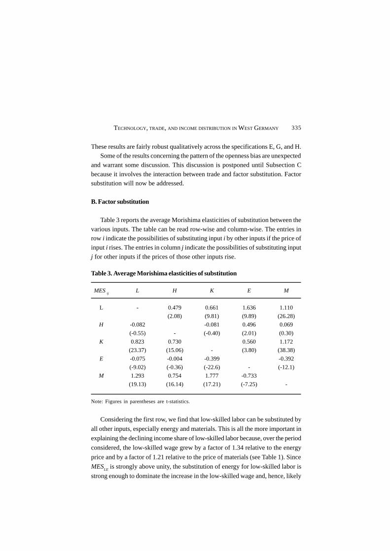
335 TECHNOLOGY, TRADE, AND INCOME DISTRIBUTION IN WEST GERMANY
These results are fairly robust qualitatively across the specifications E, G, and H.Some of the results concerning the pattern of the openness bias are unexpected
and warrant some discussion. This discussion is postponed until Subsection C
because it involves the interaction between trade and factor substitution. Factorsubstitution will now be addressed.
B. Factor substitution
Table 3 reports the average Morishima elasticities of substitution between the
various inputs. The table can be read row-wise and column-wise. The entries inrow i indicate the possibilities of substituting input i by other inputs if the price of
input i rises. The entries in column j indicate the possibilities of substituting input
j for other inputs if the prices of those other inputs rise.
Table 3. Average Morishima elasticities of substitution
MES ij
L H K E M
L - 0.479 0.661 1.636 1.110
(2.08) (9.81) (9.89) (26.28)
H -0.082 -0.081 0.496 0.069
(-0.55) - (-0.40) (2.01) (0.30)
K 0.823 0.730 0.560 1.172
(23.37) (15.06) - (3.80) (38.38)
E -0.075 -0.004 -0.399 -0.392
(-9.02) (-0.36) (-22.6) - (-12.1)
M 1.293 0.754 1.777 -0.733
(19.13) (16.14) (17.21) (-7.25) -
Note: Figures in parentheses are t-statistics.
Considering the first row, we find that low-skilled labor can be substituted by
all other inputs, especially energy and materials. This is all the more important in
explaining the declining income share of low-skilled labor because, over the period
considered, the low-skilled wage grew by a factor of 1.34 relative to the energy
price and by a factor of 1.21 relative to the price of materials (see Table 1). Since
MESLE
is strongly above unity, the substitution of energy for low-skilled labor is
strong enough to dominate the increase in the low-skilled wage and, hence, likely

JOURNAL OF APPLIED ECONOMICS336
played a role in the decline of the low-skilled share.17 The same applies to thesubstitution of materials for low-skilled labor, even though to a smaller extent.18
The situation is different for high-skilled labor (second row). High skilled labor
cannot be substituted by any other input except energy19, and the substitutionelasticity vis-a-vis energy is below unity. Thus, even though the high-skilled wage
grew by a factor of 1.31 relative to the energy price, substitution of energy for
high-skilled labor is not pronounced enough to hurt the high-skill share.20
As evidenced in the third row, capital can be substituted by all other inputs,
but only relative to materials is the substitution elasticity above unity. Since the
user cost of capital grew by a factor of 1.11 relative to the price of materials,substitution of materials for capital took place and had an adverse effect on the
capital share.
Since we are interested mainly in the distribution of income (value-added), notin factor shares in general, we will not discuss the fourth and the fifth rows in
depth.21 Turning to a column-wise analysis and considering the first column, we
find that low-skilled labor could - technologically - substitute capital and materials,but not high-skilled labor and energy. However, the former possibilities are irrelevant
because the low-skilled wage grew stronger than the prices of capital and materials.
High-skilled labor (second column) is able to substitute - to some degree - all other
17 The substitution of energy - especially electricity - for low-skilled labor involves, forinstance, what is usually called ‘automatization’ of industrial processes.
18 Falk and Koebel (2001) also find a substitution of intermediates for low-skilled labor. Theyspeculate that this may indirectly reflect the impact of foreign competition in that semifinishedgoods produced by foreign labor are substituted for domestic unskilled labor. Their approachdoes not address the impact of trade directly.
19 This results entails, especially, a confirmation of the ‘capital-skill complementarity’hypothesis. The substitution of energy for high-skilled labor concerns, e.g., electronic dataprocessing.
20 It may be noted that the substitutability of high-skilled labor is noticeably higher towards theend of the time span than the average across time. However, even in 1994 the elasticitybetween high-skilled labor and energy is the only one which is significant.
21 With respect to the fourth row, it may, however, be noted that we find all inputs to becomplementary to energy, implying a positive own-price elasticity of energy. This could be dueto shortcomings in the model specification, but we deem an explanation in terms of thecomposition of energy more appropriate: The period under consideration was characterized bya pronounced substitution of electricity for fuels (partly related to the process of ‘automatization’mentioned in footnote 17). This means, there was a quality improvement in the energyaggregate to the effect that demand increased even if the price of the aggregate rose.

337 TECHNOLOGY, TRADE, AND INCOME DISTRIBUTION IN WEST GERMANY
inputs except energy, whereas capital (third column) can substitute low-skilledlabor and especially materials. The latter (technological) possibility is not relevant,
given the evolution of the prices (see Table 1), but a substitution of capital for low-
skilled labor did occur, even though it did not hurt the low-skilled share (due to theelasticity being below unity).
C. Discussion
We will now discuss our findings from Subsection A concerning the effects of
increased openness on factor shares. Especially, the result that increased opennessraises the share of low-skilled labor may be seen as being in contrast to previous
findings (Fitzenberger 1999, Neven and Wyplosz 1999) and needs some clarification.
In order to understand this and related results, it is useful to differentiate theoverall impact of trade on factor shares (or likewise factor demand) into (a) an
effect relating to trade-induced changes in the composition of aggregate output
(due to comparative advantage) and (b) an effect relating to the substitution ofimported inputs for domestic inputs (due to input price differences). Our result
relates only to issue (a), and additional evidence will be cited in support of this
result. With respect to issue (b), this effect may in fact have worked to thedisadvantage of low-skilled labor, but cannot be identified from our data. The
overall effect may have been negative.22
With respect to issue (a) we are, unfortunately, unable to differentiate theeffect of trade into separate effects of imports and exports. From a conceptual
point of view, it can be said that a positive effect of increased openness on the
shares of low-skilled labor and of energy would be consistent with low-skillintensive or energy intensive industries displaying relatively high export growth.
Likewise, it would be consistent with these industries facing a low (or decreasing)
degree of import competition. The converse applies in the case of the negativeeffects of openness on the shares of capital, high-skilled labor, and materials, i.e.
the industries which are intensive with respect to these inputs should be
characterized by relatively low export growth or increasing import competition, orboth.
22 Previous studies which found that trade has an adverse effect on low-skilled labor in WestGermany (Fitzenberger 1999, Neven and Wyplosz 1999) were unable to differentiate betweenthese partial effects because their scope was confined to different types of labor (and possiblycapital). In the current study, both of these issues are addressed jointly, especially by includingintermediate inputs (energy and materials).

JOURNAL OF APPLIED ECONOMICS338
From an empirical point of view, our finding concerning the negative impact of
openness on the share of high-skilled labor is indeed consistent with the fact that
West German import prices declined most for skill-intensive industries (Neven and
Wyplosz 1999), implying increasing import competition for high-skilled labor. An
observation consistent with increasing import competition for high-skilled labor is
the fact that the share of high-technology products in German imports increased
over the period 1980-1994 from 43.1 to 53.6 percent (Heitger, Schrader and Stehn
1999).
Given the (almost) steady increase of the German trade surplus23, it would be
inappropriate to focus exclusively on the import side. With respect to the relationship
between factor intensities and export growth, we can refer to a companion paper
(Welsch 2004) which presents the results of a regression exercise involving 26
manufacturing industries for which data on the skill structure of labor are available.24
These regressions show that export growth has been higher in low-skill intensive
industries than in high-skill intensive industries. In addition, export growth is
positively related to intensity with respect to intermediate inputs (materials and
energy) and capital.
The question arises how this phenomenon can be explained. In Subsection A
we found evidence of low-skill-saving technological progress. This obviously
contributed to reducing production costs in low-skill intensive industries. In
addition, in Subsection B we found evidence of a substitution away from expensive
low-skilled labor towards, especially, materials and energy. This reduced production
costs further. As a consequence, the competitiveness of low-skill intensive
industries rose and, via this channel, increased openness benefited low-skilled
labor. This does not, however, imply that the overall effect of openness on low-
skilled labor was favorable, since the intermediate inputs which were substituted
for low-skilled labor include (an unknown fraction of) imported intermediates.25
In contrast to low-skilled labor, high-skilled labor is hardly prone to substitution
23 The EX/GDP ratio grew by a factor of 1.6 in 1976-1994, whereas IM / GDP grew by a factorof 1.4.
24 These are the industries examined by Falk and Koebel (2001).
25 See Falk and Koebel (2001) for a similar argument. Since the substitution of intermediateinputs for low-skilled labor may involve imported intermediates, low skilled labor may havebeen hurt by openness via this channel, but not via the impact of openness on the compositionof aggregate output. This issue is discussed in the following Subsection.

339 TECHNOLOGY, TRADE, AND INCOME DISTRIBUTION IN WEST GERMANY
by less expensive inputs (see Table 3), and technological progress is high-skill
using rather than high-skill saving. Thus, even though the growth of high-skilled
wages was slightly less than the growth of low-skilled wages (see Table 1), high-
skill intensive industries may have lost in competitiveness, relative to low-skill
intensive industries, and may thus have benefited less from increased access to
world markets.
As concerns capital, its price rose less than the two types of wages. In addition,
the Morishima elasticities of capital (Table 3) suggest that some substitution of
materials for capital took place, raising the competitiveness of capital-intensive
industries. This explains why these industries also had a relatively favorable export
performance, as pointed out above. However, given that the price of capital
increased relatively slowly, this effect was apparently not strong enough to have
an impact on the income share of capital. In other words, the fact that capital
intensive industries had a favorable export performance is not in contradiction
with our result that increased openness affected the income share of capital
negatively.
D. Weighting the roles of prices, technology, and trade
We now proceed by decomposing the variation in factor shares into their
various components. The decomposition actually carried out slightly deviates
from the decomposition described in (7) in so far as we cannot differentiate the
effect of increasing trade orientation into an import-related and an export-related
effect and must content ourselves with an overall openness effect.
We first consider the longer-term changes in factor intensities according to
equation (7), as presented in Table 4.
We see that except for capital the estimated factor shares are not very sensitive
to the models considered (letters E, G, and H refer to the models introduced in
Table 2). Moreover, all models agree in that substitution reduced the share of both
low-skilled and high-skilled labor as well as capital and raised the share of
intermediates, while the share of energy was practically unaffected by substitution
processes. With respect to all inputs the bulk of the factor share changes comes
from technological progress. Trade-related changes in output composition played
a minor role.
If we consider the short-term variation and its composition along the lines of
equation (8), we obtain the results shown in Table 5. In this table, the interaction

JOU
RN
AL O
F AP
PLIE
D EC
ON
OM
ICS
340
Table 4. Decomposition of the change in factor share
ii ss ˆ/ˆ∆ Substitution Progress Trade
E G H Mean E G H Mean E G H Mean E G H Mean
Ls -0.19 -0.20 -0.20 -0.19 -0.08 -0.05 -0.06 -0.06 -0.16 -0.17 -0.16 -0.16 0.05 0.02 0.02 0.03
Hs 0.28 0.28 0.27 0.28 -0.05 -0.01 -0.01 -0.02 0.37 0.31 0.31 0.33 -0.04 -0.03 -0.03 -0.03
Ks 0.08 0.10 0.11 0.10 -0.02 -0.09 -0.08 -0.06 0.13 0.21 0.21 0.18 -0.03 -0.02 -0.02 -0.02
Es -0.20 -0.21 -0.21 -0.21 -0.01 0.003 0.003 -0.00 -0.25 -0.33 -0.33 -0.30 0.05 0.12 0.12 0.10
Ms 0.05 0.05 0.06 0.05 0.05 0.05 0.05 0.05 0.02 0.02 0.02 0.02 -0.02 -0.02 -0.02 -0.02

341 TECHNOLOGY, TRADE, AND INCOME DISTRIBUTION IN WEST GERMANY
Table 5. Decomposition of the variation in factor shares (percent)
Substitution Progress Trade
E G H Mean E G H Mean E G H Mean
Ls 23.3 18.3 15.9 19.2 70.1 79.9 82.2 77.4 6.7 1.8 2.0 3.5
Hs 50.0 53.5 51.5 51.7 49.5 46.1 48.1 47.9 0.5 0.4 0.4 0.4
Ks 42.5 35.8 27.8 35.4 54.8 63.6 71.6 63.3 2.7 0.6 0.6 1.3
Es 80.5 69.7 68.8 73.0 18.6 26.5 27.2 24.1 0.9 3.8 4.0 2.9
Ms 91.4 90.3 89.7 90.5 4.1 6.2 6.4 5.5 4.5 3.5 4.0 4.0
effects shown in (8) are neglected and the substitution, progress, and trade effects
are shown as percentages of their sum.26
Again, the three models do not differ fundamentally in the role they attribute tothe various driving forces. We will focus on the mean across the various models.
The probably most outstanding result is that trade-induced structural change
generally plays a minor role, which, however, tends to be larger for the intermediateinputs than for the primary inputs. Among the primary inputs, low-skilled labor is
more affected by trade than are high-skilled labor and capital. The dominating
influence on the shares of the intermediate inputs comes from substitution, whereastechnology bias (progress) is of lesser importance. The converse is true for low-
skilled labor and capital, whereas the contributions of substitution and progress
to the variation of the high-skill share are almost equal.The result that trade-induced structural change plays only a minor role for
primary factor shares is consistent with findings that even in the United States
changes in the industrial structure - irrespective of their cause (trade or other) -account only for a small fraction (16 percent) of changes in the structure of labor
demand (Murphy and Welch 1993). On the other hand, a relatively large role played
by technology bias is necessary for explaining rising skill-intensity in the face ofrising skill-prices (see Gottschalk and Smeeding 1997).
With respect to the substitution component, a few more specific comments
may be instructive. The contribution of this component is relatively large in thecase of high-skilled labor and smaller in the cases of low-skilled labor and capital.
One reason for the small contributions of substitution in the cases of low-skilled
26 More specifically, substitution refers to )ˆvar()ˆvar()ˆvar()ˆvar()ˆvar( 54321 sssss ++++ in the
notation of Section II.C.

JOURNAL OF APPLIED ECONOMICS342
labor and capital is that the own-price effects are very low in the case of these twoinputs, i.e. the effects on the respective factor shares of changes in the two
corresponding prices are just offset by induced quantity changes in the opposite
direction. The most important price-related impact on the low-skill share comesfrom the price of energy, whereas the impact of the materials price on the low-
skilled share are much smaller. For capital, the most important price-related driver is
the price of low-skilled labor, i.e. the increase in the low-skilled wage led to asubstitution of capital for low-skilled labor, resulting in an increase of the capital
share. Similarly, the share of high-skilled labor also benefited from a substitution of
high-skilled labor for low-skilled labor, but the dominating price-related influenceon the high-skill share is the change (increase) in the high-skill wage (own-price
effect), which is far from being compensated by induced quantity changes, due to
the low degree of substitutability of high-skilled labor.27
An open question is, to what extent the substitution of intermediates for low-
skilled labor comprises imported intermediates. As mentioned above, the impact of
the energy price on the low-skilled share is stronger than the impact of the materialsprice. In fact, given our estimates of the degrees of substitutability, the most
important intermediate substitute for low-skilled labor is energy. Moreover, it is
likely that low-skilled labor was mainly substituted by electricity (automatizationof production processes), rather than by fuels. This view is also consistent with
the result that the capital share benefited from the increase in the low-skilled wage:
automatization mainly encompasses the substitution of capital and electricity forlow-skilled labor.28 Since electricity is basically non-traded (especially over the
period considered), we are thus led to the conjecture that at least one type of the
substitution of intermediate inputs for low-skilled labor was a purely domesticphenomenon.
This reasoning is -admittedly- somewhat speculative. More precise statements
on the role of trade in the substitution of intermediates for low-skilled labor areimpossible to derive from our analysis.29
27 With respect to the intermediate inputs, the most important price-related driver of factorshares is the energy price. Given the low degree of substitutability of energy (see Table 3),energy price changes have a strong impact on the energy share. In addition, given thecomplementarity relationship between materials and energy, energy price changes also have astrong impact on the share of materials.
28 Recall from Table 3 that capital is a Morishima complement to energy (i.e. MESEK
< 0),which applies especially to electricity.
29 Note that even though the fraction of imported intermediates in total intermediates is

343 TECHNOLOGY, TRADE, AND INCOME DISTRIBUTION IN WEST GERMANY
IV. Conclusions
This paper has examined the determinants of functional income distribution in
West Germany over the period 1976-1994. Our approach was to estimate a completesystem of factor share equations for low-skilled labor, high-skilled labor, capital,
energy, and materials, taking account of biased technological progress and
increasing trade-orientation.Our basic conclusions with respect to the roles of trade and technology are
that the shares of capital and high-skilled labor benefit from biased technological
progress, whereas the share of low-skilled labor is adversely affected bytechnological progress. The effect of technology bias on the two labor shares is
enhanced by substitution of intermediate inputs for low-skilled labor, which is
almost absent in the case of high-skilled labor. To the extent that this substitutioninvolves imported intermediates, increased openness hurts low-skilled labor. Trade-
induced changes in the composition of aggregate output tend to mitigate these
effects, due to the relatively favorable export performance of low-skill intensiveindustries. The latter, in turn, is explicable by non-neutral technological progress
and the increasing use of intermediates enhancing the competitiveness of low-
skill intensive industries.From a methodological point of view, our inclusion of the complete set of
inputs proved to be rewarding as it allowed to separate the effect of substitution
processes from trade-induced structural change. Since the latter influence turnedout to have a positive impact on the income share of low-skilled labor, trade seems
to have hurt low-skilled labor mainly via the substitution of imported intermediates
for low-skilled labor. The extent to which this was the case is difficult to quantify.However, the overall contribution of trade to the year-to-year-variation in the
factor shares of the primary inputs is small and vastly dominated by the contribution
of biased technological progress.
References
Abraham, Katharine G., and Susan N. Houseman (1995), “Earnings inequality in
Germany”, in R. B. Freeman and L. Katz, eds., Differences and Changes in
Wage Structures, Chicago, University of Chicago Press.
known, we are unable to identify the amount of imported intermediates which serve as substitutesfor low-skilled labor (or any other domestic input).

JOURNAL OF APPLIED ECONOMICS344
Berman, Eli, John Bound, and Stephen Machin (1998), “Implications of skill-biased
technological change”, Quarterly Journal of Economics 113: 1245-1279.
Berndt, Ernst R. (1991), The Practice of Econometrics: Classic and Contemporary,
Reading, MA, Addison-Wesley.
Blackorby, Charles, and Robert R. Russell (1989), “Will the real elasticity of
substitution please stand up? A comparison of the Allen/Uzawa and Morishima
elasticities”, American Economic Review 79: 882-888.
Burda, Michael C., and Barbara Dluhosch (2002), “Cost competition, fragmentation
and globalization”, Review of International Economics 10: 424-441.
Christensen, Laurits R., Dale W. Jorgenson, and Lawrence J. Lau (1973),
“Transcendental logarithmic production frontiers”, Review of Economics and
Statistics 55: 28-45.
Davis, Donald Ray (1998), “Technology, unemployment, and relative wages in a
global economy”, European Economic Review 42: 1613-1633.
Falk, Martin, and Bertrand Koebel (2001), “A dynamic heterogeneous labour demand
model for German manufacturing”, Applied Economics 33: 339-348.
Fitzenberger, Bernd (1999), “International trade and the skill structure of wages
and employment in West Germany”, Jahrbücher für Nationalökonomie und
Statistik 219: 67-89.
Freeman, Richard B. (1995), “Are your wages set in Beijing?”, Journal of Economic
Perspectives 9: 15-32.
Frondel, Manuel, and Christoph M. Schmidt (2002), “The capital-energy
controversy: An artifact of cost shares?”, The Energy Journal 23: 53-79.
Geishecker, Ingo (2002), “Outsourcing and the demand for low-skilled labour in
German manufacturing: New evidence”, Discussion Paper 313, DIW.
Gottschalk, Peter, and Timothy Michael Smeeding (1997), “Cross-national
comparisons of earnings and income inequality”, Journal of Economic
Literature 35: 633-687.
Heitger, Bernhard, Klaus Schrader, and Jürgen Stehn (1999), Handel, Technologie
und Beschäftigung, Tübingen, Mohr Siebeck.
Kölling, Arnd, and Thorsten Schank (2002), “Skill-biased technological change,
international trade and the wage structure”, mimeo, Institute for Employment
Research, Nuremberg.
Krugman, Paul (1995), “Growing world trade: Causes and consequences”,
Brookings Papers on Economic Activity issue 1: 327-362.
Leamer, Edward E. (1996), “Wage inequality from international competition and

345 TECHNOLOGY, TRADE, AND INCOME DISTRIBUTION IN WEST GERMANY
technological change: Theory and country experience”, American Economic
Review 86: 309-314.Machin, Stephen, and John van Reenen (1998), “Technology and changes in skill
structure: Evidence from seven OECD countries”, Quarterly Journal of
Economics 113: 1215-1244.Murphy, Kevin M., and Finis R. Welch (1993), “Industrial change and the rising
importance of skill”, in S. Danziger and P. Gottschalk, eds., Uneven Tides:
Rising Inequality in America, New York, Russell Sage Foundation.Neven, Damien, and Charles Wyplosz (1999), “Relative prices, trade, and
restructuring in European industry”, in M. F. Dewatripont, ed., Trade and Jobs
in Europe: Much Ado about Nothing?, Oxford, Oxford University Press.OECD (1996), Flows and Stocks of Fixed Capital, Paris.
Reinberg, Alexander, and Markus Hummel (1999), “Bildung und beschäftigung im
vereinten Deutschland“, Beiträge zur Arbeitsmarkt- und Berufsforschung no.226, Nuremberg.
Richardson, John David (1995), “Income inequality and trade: How to think, what
to conclude”, Journal of Economic Perspectives 9: 33-56.Saeger, Steven Schaal (1997), “Globalization and deindustrialization: Myth and
reality in the OECD”, Weltwirtschaftliches Archiv 133: 549-608.
Statistisches Bundesamt (1994), Volkswirtschaftliche Gesamtrechnungen,Fachserie 18, Reihe 2, Stuttgart.
Steiner, Viktor, and Karsten Wagner (1998), “Relative earnings and the demand for
unskilled labor in West German manufacturing”, in S. W. Black, ed.,Globalization, Technological Change, and Labor Markets, Dordrecht, Kluwer
Academic Publishers.
Welsch, Heinz (2004), “Skill intensity and export growth in West Germanmanufacturing”, Applied Economics Letters 11: 513-515.

347 PRICE DISCRIMINATION AND MARKET POWER IN EXPORT MARKETS
Journal of Applied Economics. Vol VIII, No. 2 (Nov 2005), 347-370
PRICE DISCRIMINATION AND MARKET POWERIN EXPORT MARKETS:
THE CASE OF THE CERAMIC TILE INDUSTRY
FRANCISCO REQUENA SILVENTE *
University of Valencia
Submitted January 2003; accepted May 2004
This paper combines the pricing-to-market equation and the residual demand elasticityequation to measure the extent of competition in the export markets of ceramic tiles, whichhas been dominated by Italian and Spanish producers since the late eighties. The findingsshow that the tile exporters enjoyed substantial market power over the period 1988-1998,and limited evidence that the export market has become more competitive over time.
JEL classification codes: F14, L13, L61
Key words: price discrimination, market power, export markets, ceramic tile industry
I. Introduction
Since the late 1980s the global production of exported ceramic tiles has been
concentrated in two small and well-defined industrial districts, one in Emilia-
Romagna (Italy) and another in Castellon de la Plana (Spain). In 1996 these twoareas constituted above 60 percent of the world export value of glazed ceramic
tiles, and in several countries these exports represented over 50 percent of national
consumption. Furthermore, Italian and Spanish manufacturers exported more than50 percent of their production while other major producers, such as China, Brazil
and Indonesia, exported less than 10 percent.
* Correspondence should be addressed to University of Valencia, Departamento de EconomíaAplicada II, Facultad de Ciencias Económicas y Empresariales, Avenida de los Naranjos s/n,Edificio Departamental Oriental, 46022, Valencia, Spain; e-mail [email protected]: Tony Venables, John Van Reenen, Chris Milner, James Walker, a refereeand Mariana Conte Grand, co-editor of the Journal, provided helpful comments for which I amgrateful. I also thank the participants of conference at 2001 ETSG (Glasgow, Scotland) andseminars during 2002 at LSE (London, UK) and Frontier Economics (London, UK). This is aversion of Chapter 4 of my thesis at the London School of Economics. I am grateful forfinancial support from the Generalitat Valenciana (GRUPOS03/151 and GV04B-070.)

JOURNAL OF APPLIED ECONOMICS348
Although it is widely accepted that local competition is aggressive in theItalian and Spanish domestic markets, it is not clear how much competition there is
between Italian and Spanish exporter groups in international markets. On one
hand, market segmentation may have prevented the strong domestic competitionapparent in domestic markets from occurring in export destinations. In addition, a
leadership position of some producers might have allowed them to act as
monopolists in some destinations. On the other hand, the increasing presence ofboth exporter groups in all exports markets may have eroded the market power of
established exporters over time. As far as I know, this study is the first to estimate
international mark-ups with data for two exporter groups that clearly dominate allthe major import markets (a case of two-source-countries with multiple destinations).
To measure the extent of competition in the export markets of the tile industry,
I propose a simple two-step approach. In the first step, I use the pricing-to-marketequation (Knetter 1989) to estimate the marginal cost functions of both Italian and
Spanish exporters. Indeed, this is a methodological contribution of the paper since
previous research measuring market power in foreign markets has relied on crudeproxies to measure the supply costs of the industry (such as wholesale price index
or some input price indices).1 In the case of this study, since Italian and Spanish
producers are concentrated in the same area within each country, I can reasonablyassume that firms in each exporter group face the same marginal cost function. In
the second step, I identify which markets each exporter group had market power in,
and the extent to which that market power was affected by the presence of othercompetitors, using the residual demand elasticity equation and the marginal cost
estimates obtained in the first step.
My findings show that the tile exporters enjoyed substantial market powerover the period 1988-1998, with weak evidence that the export market has become
more competitive over time. There is strong evidence of market segmentation and
pricing-to-market effects in the export markets of tiles. In particular, exporters adjustmark-ups to stabilise import prices in the European destinations, while they apply
a “constant” mark-up export price policy in non-European markets. This finding
may be explained by greater price transparency of the European destinations, inline with what Gil-Pareja (2002) finds for other manufacturing sectors. The results
using the residual demand elasticity equation show positive price-above-marginal
1 See Aw (1993), Bernstein and Mohen (1994), Yerger (1996), Bughin (1996), Steen andSalvanes (1999), Goldberg and Knetter (1999), among others. In some papers cost proxies arederived at national rather than industrial level of aggregation.

349 PRICE DISCRIMINATION AND MARKET POWER IN EXPORT MARKETS
costs occur in half of the largest destination markets. Accounting data of bothsource countries provide support for this outcome (Assopiastrelle 2001). Following
Goldberg and Knetter (1999), I relate the extent of each exporter group’s mark-up to
the existence of “outside” competition in each destination market, finding thatonly Spanish mark-ups are sensitive to Italians’ market share. Moreover, both
Spanish and Italian mark-ups are insensitive to the market quota of domestic rivals,
suggesting that these two exporters group have capacity to differentiatesuccessfully their product in the international markets.
The remainder of the paper is structured as follows. Section II briefly describes
the ceramic tile industry. Section III introduces the theoretical framework and itsempirical implementation. Section IV examines the data, specification issues and
the results, and Section V provides conclusions.
II. The ceramic tile market
Ceramic tiles are an end product that is produced by burning a mixture ofcertain non-metal minerals (mainly clay, kaolin, feldspars and quartz sand) at very
high temperatures. Tiles have standardised sizes and shapes but have different
physical qualities, especially in terms of surface hardness. Tiles are used as abuilding material for residential and non-residential construction with the non-
residential property being the primary source of demand.
Italy, the world leader, produced 572 million square metres in 1997, comparedwith only 200 million square metres in 1973. Over the same period exports rose from
30% to 70% of total production. Overall, Italy’s tile industry accounts for 20% of
global output and 50% of the world export market. The sources of comparativeadvantage in Italy in the seventies and eighties comes from a pool of specialised
labour force, access to high quality materials and a superior technological capacity
to develop specific machinery for the tile industry.2
Tile makers elsewhere are catching up with the Italians.3 In 1987 Italy was
clearly the largest producer and exporter of ceramic tiles in the world. Spanish
2 Porter (1990) attributes the success of Italian tile producers in the international markets tofierce domestic competition coupled with the high innovation capacity of machinery engineersto reduce production costs. Porter’s analysis covers the period 1977-1987 in order to explainthe success of Italian producers abroad. Our study starts in 1988, year in which Spain and otherlarge producers start gaining market quota to Italy in most export markets.
3 The documentation of the facts in this section relies heavily on ASCER, Annual Report 2000,and The Economist, article “On the tiles”, December 31st, 1998.

JOURNAL OF APPLIED ECONOMICS350
production started competing against Italian producers in the late 1970s, althoughthe technological and marketing superiority of Italian producers was very clear. In
1977 Spanish production was equivalent to one-third that of Italy. In 1987 Spain’s
production was only one half that of Italy, but by 1997 Spanish production wasequivalent to 85% of Italian output. In the same year, exports represented 52% of
total Spanish production. The success of Spanish producers may be attributed to
the use of high quality clay and pigments to create a new market niche in large floortiles, and to the control of marketing subsidiaries by manufacturing companies.
The abundant supply of basic materials, low labour costs and the sheer size of
population are amongst the most important factors that led to the expansion of theceramic tile industry in China, Brazil, Turkey and Indonesia. However, the expansion
in production by developing countries is strongly orientated to their respective
domestic markets. In 1996 China’s production was slightly below that of Italy, butits exports were only 5% of total production, while Brazil, Indonesia and Turkey
exported 14%, 12% and 11% of their output, respectively. Moreover the destination
markets of developing countries are mainly neighbour countries, showing thedifficulties of these countries to penetrate other destination markets.
There are two reasons why Italians and Spanish tile makers maintain their
leadership position in the export markets. On the one hand, because of a superiorown-developed engineering technology that allows Italian and Spanish producers
to elaborate high-quality tiles compared to competitors in developing countries.
The best example is the high-quality porcelain ceramic tile, a product in whichItalian and Spanish exporters are the absolute world leaders. On the other hand,
because of the innovative designs that differentiate the product from other
competitors. High quality ceramic tiles with the logos “Made in Italy” and “Madein Spain” add value to what is basically cooked mud.
Table 1 displays the distribution of the ceramic tile exports among the 19 largest
destinations (accounting for 77% of world import market). Three features aboutthese export markets are worth mentioning since they have important implications
in the later empirical analysis. First, in almost all countries, imports represent more
than 60% of total domestic consumption, and the import/consumption ratio isabove 75% in the majority of cases. Second, in all but one market (Hong Kong),
either Italy or Spain is the largest exporter, and in fourteen of the nineteen markets
one of the two dominant exporting nations is also the second largest exporter.Furthermore, in all the destinations, the sum of Italian and Spanish products is
above 50% of total imports and, in some cases, the ratio is above 95% (Greece,
Israel and Portugal). Third, in almost every market, Italian and Spanish exporters

35
1 P
RIC
E DIS
CR
IMIN
ATIO
N AN
D MA
RK
ET P
OW
ER IN E
XP
OR
T MA
RK
ET
S
Table 1. Import shares and main exporters in the largest destination markets in 1996
Imports Imports/Country (thous. Consump. (%) (%) (%) (%)
m2) (%)
Germany 145,159 78 Italy 68 Spain 9 France 7 Turkey 7USA 87,743 60 Italy 32 Mexico 24 Spain 18 Brazil 10France 75,674 63 Italy 61 Spain 15 Germany 6 Netherlands 5Poland 32,262 64 Italy 55 Spain 28 Czech Rep. 9 Germany 4UK 29,382 78 Spain 38 Italy 21 Turkey 12 Brazil 7Greece 27,577 91 Italy 62 Spain 33 Turkey 2 Others 3Hong Kong 27,008 93 China 33 Spain 29 Italy 20 Japan 10Belgium 22,518 98 Italy 53 Spain 14 Netherland 10 France 8Netherlands 20,453 78 Italy 39 Spain 18 Germany 16 Portugal 4Singapure 19,422 100 Italy 34 Spain 31 Malaysia 17 Indonesia 7Saudi Arabia 19,276 78 Spain 61 Turkey 11 Italy 10 Libanon 6Australia 17,703 84 Italy 54 Spain 11 Brazil 7 Indonesia 5Israel 17,009 74 Spain 55 Italy 34 Turkey 4 Others 7Austria 16,963 99 Italy 79 Germany 9 Spain 4 Czech Rep. 3Portugal 15,083 28 Spain 97 Italy 2 Others 1Russia 14,044 21 Spain 27 Italy 24 Turkey 14 Germany 5Canada 13,450 88 Italy 43 Turkey 14 Brazil 12 Spain 11South Africa 12,418 57 Italy 43 Spain 17 Taiwan 13 Brazil 10Switzerland 10,485 87 Italy 69 Germany 10 Spain 6 France 5
Source: Own elaboration using data from ASCER, Informe Anual 2000.
1st
exporter2nd
exporter
3rd
exporter
4th
exporter

JOURNAL OF APPLIED ECONOMICS352
face competition from a neighbouring exporter group. Germany has a notable marketshare in the Netherlands, Austria and Switzerland while Turkey has a significant
presence in Greece and Saudi Arabia.
III. The theoretical framework
For a “normal” demand curve on an international market k in a particular periodt, X
kt = X
kt (P
kt, Z
t), the supply of tiles by a profit-maximising monopolistic exporter
selling to market k is given by the equilibrium output condition, where marginal
revenue equals marginal cost,
where Pk is the product price FOB in source country’s currency, ε
k is the price
elasticity of demand facing all firms in market k, and λ is the marginal cost ofproduction (all at time t). As written, it states that price in source country’s currency
is a mark-up over marginal cost determined by the elasticity of demand in the
destination market.
A. The pricing-to-market equation
Knetter (1989, 1993) showed that equation (1) can be approximated for cross-
section time series data by
J = I , S, (2)
where J refers to source country (here, Italy or Spain), k refers to each of the
destination markets and t refers to time. The export price to a specific marketbecomes a function of the bilateral exchange rate expressed as foreign currency
units per domestic currency, ekt; a destination-specific dummy variables, θ
k,
capturing time-invariant institutional features; and, a set of time dummies, λt, that
primarily reflects the variations in marginal costs of each exporter group. A random
disturbance term, ukt, is added to account for unobservable factors by the researcher,
or for measurement error in the dependent variable.4
tkt
ktktP λ
εε
−
=1
(1)
,lnln Jkt
Jt
Jk
Jkt
Jk
Jkt ueP +++= λθβ
4 Sullivan (1985) defined the conditions under which the use of industry-level data can be usedto make inferences about the extent of market segmentation using equation (1): (i) the industry
,

353 PRICE DISCRIMINATION AND MARKET POWER IN EXPORT MARKETS
The advantage of the pricing-to-market (PTM) equation as an indicator ofimperfect competition is its simplicity and clear interpretation. First, if θ
k ≠ 0 the null
hypothesis of perfect competition in the export industry is rejected since the exporter
firm is able to fix different FOB prices for each destination; and, if βk ≠ 0 firms may
adjust their mark-ups as demand elasticities vary with respect to its local currency
price.5
A second advantage of the PTM equation is that it allows me to test forsimilarities in pricing behaviour between exporter groups in different source-
countries by comparing the β coefficients across destinations.
A third advantage of using the PTM equation is that I can incorporate a variablethat proxies time varying marginal costs for each exporter group, under the
assumptions that it is common to all destination markets. This measure is precise
when the elasticity of demand is constant so the mark-up is fixed over marginalcost. When the mark-up is sensitive to exchange rate changes and there is a
correlation between shocks to the cost function and the exchange rates, changes
in marginal costs will affect all prices equally so there is no idiosyncratic effect onprices, and the time effects will account for the impact of such shocks. In that case,
even when the time effects obtained from the PTM equation are not the marginal
costs exactly, “… there is no reason to think that they are biased measures ofmarginal cost, only noise ones” (Knetter 1989, p. 207).
has no influence over at least one factor that changes the supply price; (ii) there is littlevariation in the perceived elasticity of demand and in the marginal costs across firms selling inthe same destination market, and that (iii) no arbitrage opportunity exists across destinations.The three conditions are satisfied in the export markets of tiles. First, exchange rate variationis exogenous to the tile industry. Second, the cost of production differences across exporters arelikely to be small since ceramic tiles are produced with a standard technology in a single regionof each of the dominant exporting countries. Third, the physical characteristics of tiles makearbitrage highly unlikely.
5 The parameter βk has also an economic interpretation as the exchange rate pass-through
effect. On the one hand, a zero value for βk implies that the mark-up to a particular destination
is unresponsive to fluctuations in the value of the exporter’s currency against the buyer’s. Onthe other hand, the response of export prices to exchange rate variations in a setting ofimperfect competition depends on the curvature of the demand schedule faced by firms. As ageneral rule, when the demand becomes more elastic as local currency prices rise, the optimalmark-up charged by the exporter will fall as the importer’s currency depreciates. Negativevalues of βk
imply that exporters are capable of price discrimination and will try to offsetrelative changes in the local currency induced by exchange rate fluctuations. Thus, mark-upsadjust to stabilise local currency prices. Positive values of β
k suggest that exporters amplify the
effect of exchange rate fluctuations on the local currency price.

JOURNAL OF APPLIED ECONOMICS354
Once the cost structure of the competitors is ascertained, we are able to measurethe extent of competition in the export markets using the residual demand elasticity
approach.
B. The residual demand elasticity equation
How exchange rate shocks are passed through to prices in itself reveals littleabout the nature of competition in product markets. Indeed, the interpretation of
the PTM coefficients depends critically on the structure of the product market
examined (Goldberg and Knetter 1997). To assess the importance of market powerin the export industry, I directly measure the elasticity of the residual demand
curve of each exporter group.
The residual demand elasticity methodology was first developed by Baker andBresnahan (1988) to avoid the complexity of estimating multiple cross-price and
own-price demand elasticities in product differentiated markets. The residual
demand elasticity approach has the advantage of summarising the degree of marketpower of one producer in a particular market in a single statistic. Recently, Goldberg
and Knetter (1999) successfully applied a residual demand elasticity technique to
measure the extent of competition of the German beer and U.S. kraft paper industriesin international markets.
Consider two groups of exporters, Italians and Spaniards, selling in a particular
foreign market (therefore we omit the subindex k). The inverse demand curveincludes the export price of the other competitor and a vector of demand shifters,
J = I, S ; R = rival , (3)
where XJ stands for the total quantity exported by the J exporter group (note that
I use the letter J to refer to Italy or Spain and the letter R to refer to rival), P is theprice expressed in destination country’s currency terms, and Z is a vector of
exogenous variables affecting demand for tile exports. The supply relations for
each exporter group are
,´ JJ
JJJJ vDXeP += λ J = I, S, (4)
where λJ reflects the variations in marginal costs of each exporter group, D´J
is the partial derivative of the demand function with respect to XJ and v J is
a conduct parameter.The estimation of the market power of each exporter group requires the estimation
),,,( ZPXDP RJJ =

355 PRICE DISCRIMINATION AND MARKET POWER IN EXPORT MARKETS
of the system of equations (3) and (4). A way to avoid estimating these equationssimultaneously is to estimate the so-called residual demand equation. The approach
does not estimate the individual cost, demand and conduct parameters, but it
captures their joint impact on market power through the elasticity of the residualdemand curve.
The first step in deriving the residual demand curve is to solve (3) and (4)
simultaneously for the price and quantities of the rival exporter group,
, J = I, S; R = rival. (5)
PR* is a partial reduced form; the only endogenous variable on the right-hand
side is XJ. The dependence of PR* and XJ arises because only the rivals’ producthas been solved out. By substituting PR* into (3), the residual demand for each
exporter group (J = I or S) is obtained:
J = I, S; R = rival. (6)
The residual demand curve has three observable arguments: the quantity
produced by the exporter group, the rival exporter group cost shifters and demand
shifters and one unobservable argument (the rivals’ conduct parameters).For each destination k, we can estimate a reduced form equation of the following
general form:
J=I, S; R= rival. (7)
Equation (7) is econometrically identified for each exporter group since cost
shifters for each exporter group are excluded arguments in their own residualdemand function. In each expression the only endogenous variable is the exported
quantity XJ. I can use both eJ and λJ as instruments since both variables affect the
exported supply of the exporter group in a particular destination independently ofother exporter groups competing in the same destination market. Exchange rate
shocks rotate the supply relation of the exporting group relative to other firms in
the market, helping us to identify the residual demand elasticity.Baker and Breshanan (1988) review the cases in which the residual demand
elasticity correctly measures the mark-up over marginal cost: Stackelberg leader
case, dominant firm model with competitive fringe, perfect competition, and marketswith extensive product differentiation. In other oligopoly models the equality
( )RRRJRR vZeXPP ,,,** λ=
( ),,,,),,( * RRRJRJJ vZeXRZPXDP λ==
,lnlnlnlnln ktktkRkt
Rk
Rkt
Rk
Jkt
Jk
Jk
Jkt vZeXP +++++= δλγβηα

JOURNAL OF APPLIED ECONOMICS356
between the relative mark-up and the estimated residual demand elasticity breaksdown. However, even in these cases, a steep residual demand curve is likely to be
a valid indicator of high degree of market power. In the ceramic tile industry, the
estimated residual demand elasticity may be a good approximation to the mark-ups, since the industry is characterised by substantial product differentiation, and
both source countries (especially Italy) have enjoyed a dominant position in the
world market.
IV. Data, estimation and results
A. The data
The data consist of quarterly observations from 1988:I to 1998:I on the valuesand quantities of ceramic tiles exports (Combined Nomenclature Code 690890)
from Spain and Italy to the largest market destinations. The prices of exports are
measured using FOB unit values. As far as I am aware, no country producesbilateral export price series, which is probably the main justification for the use of
unit value to measure bilateral export prices. The drawbacks of using unit values
as an approximation for actual transaction prices are well known. The most seriousproblems are the excessive volatility of the series and the effect on prices of
changes in product quality over time (Aw and Roberts 1988). However, any purely
random measurement error introduced by the use of unit values as a dependentvariable will only serve to reduce the statistical significance of the estimates.
The analysis includes sixteen export destinations (60 percent of world import
market): Germany, USA, France, United Kingdom, Greece, Hong-Kong, Belgium,Netherlands, Singapore, Australia, Israel, Austria, Portugal, Canada, South Africa
and Switzerland. Spanish and Italian exports represented between 48 and 99 percent
of total imports in each of these markets in 1996.6
The destination-specific exchange rate data refer to the end-of-quarter and is
expressed as units of the buyer’s currency per unit of the seller’s (unit of destination
market currency per home currency).As explained above, the exporter’s marginal cost function for ceramic tiles is
obtained directly from the estimation of the PTM equation. Demand for ceramic
tiles in each destination market is captured by two variables: building construction
6 Three large destination markets (Poland, Saudi Arabia and Russia) were excluded from ouranalysis due to data limitations.

357 PRICE DISCRIMINATION AND MARKET POWER IN EXPORT MARKETS
and real private consumption expenditure. All the series in the empirical analysisare seasonally adjusted. An Appendix contains more details about the sources
and construction of the variables for the interested reader.
B. Evidence of pricing-to-market effects
In order to assess the potential for price discriminating behaviour on the partof Italian and Spanish exporters, I start by comparing the response of export prices
to exchange rate variations in each of the major destination markets. For a
comparable export product, differences in prices across export markets can beattributable to market segmentation. If the null of perfect competition is rejected,
price discrimination is possible so exporters may enjoy market power in those
destinations.Equation (2) is estimated by Zellner’s Seemingly Unrelated Regression
technique (Zellner 1962) to improve on efficiency by taking explicit account of the
expected correlation between disturbance terms associated with separate cross-section equations. The model is estimated with two different exchange rate
measures, the nominal exchange rate in foreign currency units per home currency,
and the nominal exchange rate adjusted by the wholesale/producer price index inthe destination market. The exchange rate adjustment is made, because the optimal
export price should be neutral to changes in the nominal exchange rate that
correspond to inflation in the destination markets. Estimated coefficients of thedestination-specific dummy variables, θ
k, reveal the average percentage difference
in prices across markets during the sample period, conditional on other controls
for destination-specific variation in those prices. In practice, only (N-1) separatevalues of θ
k can be estimated in the presence of a full set of time effects.
Consequently, I will normalise the model around West Germany, the world largest
import market, and test whether the fixed effects for the other countries aresignificantly different from zero. Results for the two source-countries, Italy and
Spain, are reported in Table 2. For each destination the Table reports the estimates
of the country effects θk and the coefficient on the exchange rate β
k.
Using either exchange rate measures, the destination specific effects are
significantly different from zero in almost all the cases.7 These results provide
evidence against the hypothesis of perfect competition. Looking at the estimated
7 F-tests for the exclusion of the country effects are overwhelmingly significant: 3486 for Italyand 4970 for Spain.

JOURNAL OF APPLIED ECONOMICS358
Table 2. Estimation of price discrimination across export markets
Foreign price adjusted nominal
exchange rate
Jkθ Jkβ J
kθ Jkβ
Destination k - source country J = Italy
Germany -0.59 (0.127)*** -0.53 (0.117)***
United States -0.34 (0.037)*** 0.15 (0.150) -0.32 (0.031)*** 0.12 (0.127)
France -0.09(0.032)*** -0.90 (0.132)*** -0.14 (0.028)*** -0.71 (0.104)***
UK -0.04 (0.032) -0.25 (0.230) -0.05 (0.029)* -0.26 (0.123)* *
Greece -0.41 (0.030)*** -0.54 (0.161)*** -0.35 (0.048)*** 0.08 (0.110)
Hong-Kong -0.45 (0.037)*** -0.07 (0.148) -0.45 (0.030)*** -0.03 (0.132)
Belgium -0.12 (0.032)*** -0.23 (0.125)* -0.11 (0.030)*** -0.23 (0.124)*
Netherland -0.08 (0.032)* * -0.57 (0.126)*** -0.09 (0.030)*** -0.58 (0.131)***
Singapore -0.33 (0.037)*** -0.07 (0.180) -0.34 (0.046)*** 0.03 (0.163)
Australia -0.16 (0.033)*** 0.00 (0.168) -0.14 (0.029)*** -0.10 (0.131)
Israel -0.51 (0.030)*** -0.40 (0.121)*** -0.62 (0.044)*** -0.37 (0.095)***
Austria -0.05 (0.032) -0.57 (0.127)*** -0.09 (0.050)*** -0.56 (0.127)***
Portugal -0.37 (0.030)*** -0.35 (0.246) -0.39 (0.032)*** -0.18 (0.081)* *
Canada -0.29 (0.040)*** 1.03 (0.261)*** -0.21 (0.028)*** 0.69 (0.161)***
South Africa -0.34 (0.033)*** -0.03 (0.137) -0.29 (0.036)*** -0.35 (0.134)***
Switzerland -0.02 (0.032) -0.22 (0.114)* -0.03 (0.030) -0.24 (0.122)*
Destination k - source country J = Spain.
Germany -0.69 (0.130)*** -0.68 (0.111)***
United States -0.29 (0.034)*** 0.21 (0.137) -0.28 (0.027)*** 0.08 (0.112)
France -0.04(0.030) -0.84 (0.134)*** -0.10 (0.024)*** -0.80 (0.095)***
UK -0.01 (0.029) -0.70 (0.183)*** -0.07 (0.025)*** -0.60 (0.107)***
Greece -0.45 (0.028)*** -0.12 (0.117) -0.44 (0.043)*** 0.03 (0.101)
Hong-Kong -0.42 (0.034)*** 0.04 (0.136) -0.41 (0.026)*** -0.03 (0.116)
Belgium 0.03 (0.030) -0.24 (0.128)* 0.04 (0.026)* -0.43 (0.118)***
Netherland 0.11 (0.030)*** -0.56 (0.128)*** 0.12 (0.026)*** -0.72 (0.124)***
Singapore -0.25 (0.033)*** 0.20 (0.158) -0.29 (0.039)*** 0.30 (0.136)* *
Australia -0.14 (0.030)*** 0.34 (0.148)* * -0.11 (0.025)*** 0.03 (0.116)
Israel -0.13 (0.027)*** 0.61 (0.091)*** -0.27 (0.038)*** 0.73 (0.083)***
Austria 0.19 (0.030)*** -0.56 (0.129)*** 0.20 (0.026)*** -0.72 (0.121)***
Portugal -0.11 (0.028)*** -0.10 (0.293) -0.16 (0.028)*** -0.29 (0.073)***
Nominal exchange rate

359 PRICE DISCRIMINATION AND MARKET POWER IN EXPORT MARKETS
Canada -0.14 (0.036)*** -0.39 (0.222)* -0.17 (0.025)*** -0.37 (0.141)***
South Africa -0.24 (0.029)*** 0.92 (0.109)*** -0.22 (0.032)*** 0.81 (0.127)***
Switzerland 0.03 (0.029) 0.06 (0.112) 0.04 (0.027) 0.09 (0.115)
Note: SUR Estimation, N=41. *** , ** and * indicate significance at the 1%, 5% and 10% levelHeteroskedasticity robust standard errors in parenthesis. Exchange rate series are expressed asdestination market currency per source country currency and normalised to 1 in 1994:1.Wholesale price are used to adjust exchange rates.
Table 2. (Continued) Estimation of price discrimination across export markets
Foreign price adjusted nominal
exchange rate
Jkθ Jkβ J
kθ Jkβ
Nominal exchange rate
βk, the regression with nominal exchange rates indicates that 9 export markets for
Italy and 10 export markets for Spain violate the invariance of export prices toexchange rates implied by the constant-elasticity model (at 10 % significance level).
The regression with adjusted exchange rates increases the number of export markets
to 11 for Italy and 11 for Spain for the same significance level. There is evidence ofimperfect competition with constant elasticity of demand (θ
k ≠ 0 and β
k = 0) for
most non-European markets (see USA, Hong Kong, Singapore, Australia) in one
or another source-country. In most European destinations, tile exporters perceivedemand schedules to be more concave than a constant elasticity of demand (θ
k ≠
0 and βk < 0) revealing that exporters are able to price discriminate by offsetting the
relative price changes in the local currency price induced by exchange ratefluctuations. A plausible explanation is that tile exporters have an incentive for
price stabilization in the local currency in the European markets while there is a lack
of significant stabilisation across non-European markets. In other words, Europeandestinations are more competitive than non-European ones in the export tile
industry. Theories explaining PTM behaviour such as large fixed adjustment cost
differences across destinations (Kasa 1992) or concerns for market share varyingwith the size of the market (Froot and Klemperer 1989) seem unlikely to explain this
dichotomy in price behaviour. An alternative explanation could be the greater
price transparency in the European markets over the period 1988-1998, togetherwith the fact that the number of firms selling in the European markets is larger than
in the non-European markets. This interpretation coincides with the predictions of
the Cournot oligopoly model (Dornbusch 1987).

JOURNAL OF APPLIED ECONOMICS360
A surprising feature of our results is that destination-specific mark-upadjustment is very similar across source countries for each destination country. In
order to examine in more detail the pattern of price discrimination across destinations
we re-estimate Equation (2) under the assumption that βk = β across destination
markets (Knetter 1993). The t-statistics of the first row in Table 3 indicate that the
PTM coefficients are significantly different from zero for each exporter group. The
reported F-statistic reveals that the null hypothesis of identical PTM behaviouracross destination markets is rejected at the 5 percent level. The second row in
Table 3 offers a test of whether the identical PTM behaviour is supported across
only European destinations, leaving the non-European market coefficientsunconstrained. The last column of Table 3 offers pooled regression results. In it,
the constrained coefficients across destination markets for each source country
are additionally constrained to be the same for both source countries. The reportedF-statistic reveals that the null hypothesis of identical PTM behaviour across
source countries cannot be rejected at the 5 percent level. Therefore export price-
adjustment behaviour is different across the range of destination countries foreach source country but on aggregate both source countries have similar export
price-adjustment behaviour.
The results allow me to conclude that the export price-adjustment in responseto exchange rate variations is on average 30 percent, implying that more than half
of the exporter’s currency appreciation or depreciation are passed through to
import prices (after controlling for country-specific effects and time effects). Thelow sensitivity of domestic currency prices to changes in exchange rates provides
Table 3. Testing for identical pricing-to-market behaviour across destination
Italy Spain Pooled
Constrained βk
(all destinations) -0.256 (0.063)*** -0.304 (0.067)*** -0.292 (0.045)***
F-test F(15,584) = 21.52*** F(15,584) = 11.57*** F(1,599) = 0.46
Constrained βk
(Europe only) -0.281 (0.072)*** -0.401 (0.064)*** -0.337 (0.038)***
F-test F(8,584) = 8.41*** F(8,584) = 11.94*** F(1,592) = 2.14
Note: F-statistic tests the null hypothesis that PTM coefficient is the same across exportdestinations. For the pooled regression, F-statistics test the null that PTM coefficient is thesame for both source countries. *** indicates significance at the 1% level. Heteroskedasticityrobust standard errors in parenthesis.

361 PRICE DISCRIMINATION AND MARKET POWER IN EXPORT MARKETS
indirect evidence of the existence of positive mark-ups in the export markets oftiles. The next questions to be addressed are how much market power each tile
producers has. To do that first I need an estimate of the marginal costs of each
exporter group.
C. Estimating marginal costs
In this section, I present the estimates of the coefficients on the time dummy
variables, λt, which capture variations in marginal costs of exporters. Figure 1 plots
the indexes of the estimated time effects from the regression with price-level adjustedexchange rates for Italy and Spain.8 The estimated marginal costs of both exporter
groups are relatively flat over the sample and exhibit less volatility than producer
price indices, used in past studies to control for marginal cost changes.9 Therefore,if the time effects estimated in the PTM equation are better measures of the true
marginal cost changes, using producer price indices as a proxy probably
underestimate the role of mark-up adjustments in explaining the response of localcurrency prices of exports in relation to exchange rates changes (Knetter 1989).
D. Estimating the residual demand elasticities
Equation (7) is estimated for each of the destinations, k = 1,…16. Each equation
is in double log form so that the coefficients are elasticities. The cost shifterJtλ is
the estimated time effect of each exporter group J derived from the pricing-to-
market equations in the previous section. The demand shifters Zkt consist of a
combination of the construction index, real private consumption, the nominalexchange rate of a third competitor and a time trend.
If the exported quantity JktXln and its price are endogenously determined
through the residual demand function, then OLS provides biased and inconsistentestimates. Three-stage least squares (3SLS) is employed to estimate separately
each of the 16 systems of two equations. The exogeneity assumption of the exported
quantity is testable by comparing the 3SLS and seemingly unrelated regression(SUR) estimates using the Hausman-Wu test statistic (Hausman 1978). The choice
8 Although the estimated time effects have been normalised in Figure 1, the residual demandelasticity equation uses the actual estimated coefficients. The mean and standard deviationstatistics of the estimated time effects are (9.49, 0.070) for Italy and (6.97, 0.071) for Spain.
9 It is interesting to point out that our results are opposite to those of Knetter (1989) whofound that the estimated time effects trend upwards over the sample and exhibit higher volatility.

JOURNAL OF APPLIED ECONOMICS362
of an appropriate instrument in the 3SLS is a crucial step. It is necessary to obtain
a set of instrumental variables that are correlated with the exported quantity butnot with the error term of the residual demand function in each equation. The ideal
candidates are the cost shifters and exchange rate of the source-country, as they
have been excluded from each equation as regressors. It is easy to check that thesystem is identified due to exclusion of the cost shifter and exchange rate of the
source-country in its own equation and the possible combination of four exogenous
demand shifters in each equation.Results of my preferred specifications by 3SLS appear in Table 4. The last
column reports the p-value of the Hausman-Wu test for the null hypothesis of
exogeneity of log quantity after estimating the model with (3SLS) and withoutinstrumental variables (SUR). The null hypothesis is rejected in about half of the
specifications at 10 percent significant level, suggesting that IV techniques are
necessary to control for endogeneity in the equation system. The R2 and Durbin-Watson statistics vary substantially across destinations and source countries.
The coefficient on the log quantity directly estimates the residual demand
elasticity. If I interpret the Jkη parameters as estimates of the exporter’s group
mark-up of price over marginal cost, Italy and Spain had a significant market power
Figure 1. Estimated marginal costs for Italian and Spanish producers
96.0
106.0
116.0
126.0
136.0
146.0
88 89 90 91 92 93 94 95 96 97
Year
Wholesale price (Italy)
Wholesale price (Spain)
Estimated marginal cost (Italy)
Estimated marginal cost (Spain)

363 PRICE DISCRIMINATION AND MARKET POWER IN EXPORT MARKETS
Table 4. Measuring the residual elasticity of demand in export markets of ceramictiles
Jkη Rkβ R
kγ R2 D-W H-W
Destination k - source country J = Italy
Germany -0.362 (0.105)* * * 0.518 (0.319) -6.496 (2.177)* * * 0.37 1.75 0.1
United States-0.460 (0.196)* * 0.533 (0.280)* 5.686 (4.194) 0.49 2.31 0.00 º
France -0.363 (0.132)* * * 0.582 (0.251)* * 9.408 (3.027)* * * 0.63 1.71 0.40
UK -0.885 (1.833) 1.632 (1.011) 26.706 (19.763) 0.05 1.63 0.0 º
Greece -0.417 (0.077)* * * 0.655 (0.402) 4.342 (3.736) 0.91 1.93 0.08 º
Hong-Kong -0.718 (0.379)* -0.309 (0.271) 7.960 (7.921) 0.73 1.90 0.00 º
Belgium -0.428 (0.423) 1.792 (0.999)* 0.895 (2.600) 0.12 2.05 0.20
Netherland -0.317 (0.130)* * 0.981 (0.285)* * * 11.235 (3.980)* * * 0.45 2.22 0.01 º
Singapore -0.472 (0.355) 0.830 (0.318)* * 1.154 (6.955) 0.21 2.03 0.12
Australia -0.042 (0.111) 1.190 (0.235)* * * 4.995 (1.822)* * * 0.71 2.30 0.06 º
Israel -0.231 (0.179) 0.455 (0.620) 11.391 (7.923) 0.68 1.44 0.18
Austria -0.409 (0.237)* -0.014 (0.221) -1.602 (4.948) 0.12 1.67 0.38
Portugal -0.099 (0.073) 0.753 (0.395)* -0.839 (2.167) 0.45 1.87 0.54
Canada -0.782 (0.338)* * * -1.352 (0.354)* * * 3.017 (2.321) 0.45 1.87 0.05 º
South Africa -0.662 (1.835) 0.120 (1.923) -14.298 (18.207) 0.02 1.71 0.17
Switzerland -1.139 (0.615)* 2.510 (0.861)* * * 11.404 (5.365)* * 0.49 1.72 0.16
Destination k - source country J = Spain
Germany 0.412 (0.723) 0.854 (0.972) 8.848 (11.480) 0.04 1.25 0.12
United States-0.372 (0.134)* * * 0.483 (0.250)* 8.180 (2.927)* * * 0.69 1.73 0.00 º
France -0.135 (0.066)* * 0.718 (0.161)* * * 11.432 (2.799)* * * 0.73 2.26 0.40
UK 0.019 (0.081) 0.720 (0.282)* * 12.44 (2.771)* * * 0.67 1.24 0.01 º
Greece -0.060 (0.278) 0.518 (0.884) -1.615 (4.179) 0.58 1.64 0.08 º
Hong-Kong -0.259 (0.124)* * -0.704 (0.175)* * * 3.914 (3.143) 0.74 2.18 0.00 º
Belgium 0.111 (0.377) 0.883 (0.677) 11.172 (5.929)* 0.29 1.40 0.20
Netherland -0.466 (0.430) 0.478 (0.682) 4.410 (4.087) 0.25 1.61 0.0 º
Singapore -0.713 (0.447)* 0.597 (0.338)* 3.044 (9.333) 0.61 2.15 0.12
Australia 0.068 (0.056) 1.530 (0.139)* * * 7.262 (2.539)* * * 0.84 1.41 0.06 º
Israel -0.136 (0.078)* 0.399 (0.533) 6.890 (10.93) 0.74 2.10 0.18
Austria 0.106 (0.286) 0.369 (0.328) 2.124 (2.053) 0.00 2.28 0.38
Portugal -0.192 (0.073)* * -0.079 (0.156) -1.353 (2.511) 0.75 2.20 0.55
Canada -0.063 (0.063) -0.341 (0.419) 2.259 (7.084) 0.05 1.57 0.05 º

JOURNAL OF APPLIED ECONOMICS364
South Africa -0.145 (0.092) 0.678 (0.251)* * * 3.032 (5.763) 0.60 1.57 0.17
Switzerland -0.009 (0.132) 1.174 (0.243)* * * 14.265 (5.144)* * * 0.65 1.52 0.16
Notes: Each destination is estimated jointly for Italy and Spain using 3SLS estimator. Dependentvariable: log-price of exports in local currency. Reported independent variables are log-quantityof exports, log-exchange rate between destination country and the direct rival country, andmarginal cost of direct rival country. Additional omitted exogenous variables may include theconstruction index, log-real private consumption, time trend and log-neighbour rival exchangerate in the destination market. *** , ** and * indicate significance at the 1%, 5% and 10% level.Standard errors are reported in parentheses. P-values reported for the Hausman-Wu test (H-W)test the endogeneity of log sales ,(ln JX J=I, S). º indicates p-value < 0.10.
Table 4. (Continued) Measuring the residual elasticity of demand in export marketsof ceramic tiles
Jkη Rkβ R
kγ R2 D-W H-W
over nine and six destinations respectively. For example, the residual demand
elasticity for Italy in the three largest markets is 0.362 (Germany), 0.460 (US) and0.363 (France) corresponding to a mark-up over marginal cost between 36 and 46
percent. Although Spain shows no market power in Germany, its residual demand
elasticity for US and France are 0.372 and 0.135, respectively. Looking at the rest ofthe destinations, Italy’s mark-up over marginal cost was on average 40 percent
while Spain’s were about 10 percent. This finding is consistent with Italy having a
leadership role in the industry.The interpretation of the rest of the coefficients in each equation is unclear
since they may reflect both direct effects on demand and indirect effects through
the adjustments of a rival exporter’s group; therefore I do not report them. Columns3 and 4 in Table 4 display the estimated coefficients of the rival’s adjusted exchange
rate and marginal costs. The positive sign of the coefficients reflects the significant
role of “outside” competition in constraining the market power of a particularexporter group. In general, the coefficients of the other exporter group’s exchange
rate and marginal costs are positive (and for some destinations significant),
indicating that the market power of one or another exporter group in most destinationmarkets is constrained by the presence of the other exporter group.10
10 When I estimated the residual demand elasticity equation using the wholesale price indexinstead of the estimated marginal cost obtained from the PTM equation, the sign of thesignificant coefficients for log-exchange rate and marginal cost of direct rival country did notchange. However, the magnitude of the estimated coefficient of the log-quantity of exports

365 PRICE DISCRIMINATION AND MARKET POWER IN EXPORT MARKETS
Table 5. Relationship between residual demand elasticity and rivals’ market share
Spain Source
market country:
share Spain
Switzerland -1.139 6.2 13.0 Singapore -0.713 34.4 0.3
UK -0.885 38.3 21.5 Netherland -0.466 38.8 22.4
Canada -0.782 10.7 12.2 USA -0.372 31.8 39.9
Hong-Kong -0.718 29.3 7.4 Hong-Kong -0.259 20.0 7.4
South Africa -0.662 17.4 42.5 Portugal -0.192 1.9 72.4
Singapore -0.472 30.5 0.3 South Africa -0.145 43.1 42.5
USA -0.460 17.6 39.9 Israel -0.136 34.2 26.1
Belgium -0.428 14.1 2.1 France -0.135 61.2 36.8
Greece -0.417 32.8 9.4 Canada -0.063 43.1 12.2
Austria -0.409 3.8 1.5 Greece -0.060 62.1 9.4
France -0.363 15.3 36.8 Switzerland -0.009 69.2 13.0
Germany -0.362 8.5 22.3 UK 0.019 20.5 21.5
Netherland -0.317 18.1 22.4 Australia 0.068 54.4 16.2
Israel -0.231 54.8 26.1 Austria 0.106 79.3 1.5
Portugal -0.099 97.3 72.4 Belgium 0.111 52.8 2.1
Australia -0.042 10.9 16.2 Germany 0.412 67.7 22.3
Spearman correlation -0.15 -0.33 Spearman correlation -0.64 0.26
Pearson correlation -0.34 -0.30 Pearson correlation -0.51 0.09
Regression analysis b_Spain b_home Regression analysis b_Italy b_home
Rsq=0.13 -0.003 -0.002 Rsq=0.30 -0.007 -0.003
(0.004) (0.004) (0.003) (0.003)
Notes: Figures are obtained from Table 1 and Table 4. Market shares are for the year 1996.Figures in bold means p-value<0.10. In the regression analysis, standard errors are in parenthesis.
Source
country:
Italy
Residual
demand
Domestic
share
Domestic
share
Italy
market
share
Table 5 contains the final results of the two-step procedure used to estimate
the extent of competition in the destination markets of Italian and Spanish ceramictile exporters. Destination countries are ranked from the highest to the lowest
residual demand elasticities for each source country. If the market demand elasticities
are not very different across destinations, the residual demand elasticities measure
increased in many equations, suggesting on average greater mark-ups for both Italian andSpanish exporter groups across destination markets than the ones reported in Table 5.
Residual
demand

JOURNAL OF APPLIED ECONOMICS366
the degree of “outside” competition in each destination. To interpret the elasticities,note that the lower (in absolute value) the elasticity, the stronger the competition
that each exporter group faces from the other competitor. In the previous section
the PTM analysis showed that demand elasticities were constant for non-Europeandestinations and convex across European destinations. The rank correlations
between the market power of one exporter group and the market share of the other
exporter group are clearly negative with values of -0.34 for Italy and -0.51 for Spain,suggesting that the presence of competitors reduces the market power of the other
export group. A weaker correlation was also found between the market power of
one exporter group and the local producers’ domestic market share. In myregression analysis, reported in Table 5 (last rows), the coefficient of Italian market
share in the Spanish market power regression is negative and significant, while the
coefficient of Spanish market share in the Italian market power regression is negativebut not significant. The coefficient of domestic market share is negative but not
significant in both samples. Hence, Italian exports are strong substitutes of Spanish
tiles while the evidence is weaker in the opposite direction. Finally, domestic tilesseem to be poor substitutes for both Italian and Spanish tiles. A plausible
explanation behind these findings is the combined technological superiority and
design innovation that allow Italian and Spaniard tile makers to differentiatesuccessfully their products in the international markets.
V. Conclusions
Prior to 1987 Italian firms were the absolute world leaders in the production and
export of ceramic tiles. After 1988 the international market structure of the exportindustry changed as some developing countries attained large levels of domestically
orientated production, and Spanish producers gradually gained market quota in
the international export market.In order to characterise the market structure and conduct of Spanish and Italian
tile makers in each export market, I combine two different techniques borrowed
from the New Industrial Organisation (Bresnahan 1989). First, I measure thesensitivity of local currency prices of exported tiles to different countries with
respect to exchange rate changes. The so-called pricing-to-market equation permits
me to identify the existence of price discrimination and the similarity in the pricebehaviour of Italian and Spanish exporter groups across destination markets.
Second, I measure the response of one exporter group’s price to changes in the
quantity supplied, taking into account the supply response of the other rival

367 PRICE DISCRIMINATION AND MARKET POWER IN EXPORT MARKETS
exporter group. The so-called residual demand elasticity equation allows me toidentify the extent of competition in the international tile market by quantifying the
sensitivity of the positive mark-ups of an exporter group across destinations with
respect to the market share of its rivals.Using the pricing-to-market equation I found that the export price-adjustment
in response to exchange rate variations was on average about 30%. I also observe
that both Spanish and Italian exporters set different prices in domestic currency todifferent destination markets. The evidence of market segmentation is weaker for
European destinations compared to non-European destinations, which could be
explained by the greater price transparency associated with economic integrationwithin Europe.
The estimation of the residual demand elasticity for each exporters’ group
revealed that, across destinations, both Italian and Spanish exporters have enjoyedpositive market power during the period examined (1988-1998). On average Italian
producers obtained mark-ups of 30 percent while Spanish mark-ups were 10 percent.
The results also reveal that Italian mark-ups are less sensitive to Spanishcompetition, while the historical leadership of Italian exporters has a depressive
effect on Spanish mark-ups in many destinations.
While the findings of this paper are most relevant to researchers studyingceramic tile industry, the methodology developed contributes more generally to
the literature testing market power in export markets. Obtaining information on the
determinants of the marginal costs such as input quantities or prices presents amajor problem for researchers interested in estimating market power in an industry.
I propose a simple solution to this problem by estimating the marginal cost for
each exporter group directly from the pricing-to-market equation. I also show thattechniques developed in one-source-country/multiple-destination can be
implemented to multiple-source-countries/multiple-destinations. My current
agenda of research includes explicitly modelling the strategic behaviour betweenexporter groups for a better understanding of export pricing policies in different
periods of time, in a similar way as Kadayali (1997) did for the US photographic film
industry or Gross and Schmitt (2000) did for the Swiss automobile market.

JOURNAL OF APPLIED ECONOMICS368
Appendix
A. Export quantities and prices
Price and quantity of ceramic tiles exports came from national customs, who
collected data on the total number of squared metres and the total national currency
value of exports of ceramic tiles to each destination country. Data were kindlyprovided by Assopiastrelle and Ascer, the two national entrepreneur associations.
To ensure homogeneity in the product I selected the product registered as “CN
Code 690890” from the Eurostat-Comext Customs Cooperation CouncilNomenclature: “Glazed flags and paving, hearth or wall tiles of stone ware,
earthenware or fine pottery,..., with a surface of above 7cm2”. The value of exports
does not include tariff levies, the cost of shipping and other transportation costs.Monthly data were available for all European destinations, but Italian series for
non-European destinations are only collected on a quarterly basis. Unit values are
quarterly average prices constructed dividing the value by the quantity of tradeflows. For the monthly series unit values for each quarter were calculated as the
mean average of the corresponding three months. I reduced the volatility of the
unit values series by eliminating potential outliers, excluding in my calculationsthe monthly prices five times larger or smaller than the standard deviation of the
annual average in the corresponding year (accounting for 1% of the destination-
quarter observations in the Spanish and Italian data).
B. Exchange rates and demand variables
The data on exchange rate and wholesale price were collected from the
International Financial Statistics of the International Monetary Fund (IMF). The
destination-specific exchange rate data refer to the end-of-quarter and are expressedas units of the buyer’s currency per unit of the seller’s. The adjusted nominal
exchange rate is nominal exchange rate divided by the destination market wholesale
price level.I use quarterly data on “new building construction permits” as an indicator of
building construction demand. Data were obtained from DATASTREAM and the
original sources are OECD and National Statistics. Since some series are notavailable for all the countries, alternative proxies were utilised. Specifically, the
“Construction in GDP” for Italy and South Africa, “Work put in construction” for
Hong Kong and Austria, and the “Construction production index” for Israel. Real

369 PRICE DISCRIMINATION AND MARKET POWER IN EXPORT MARKETS
private consumption expenditures were used to proxy for the household demandof ceramic tiles. When disaggregated data were unavailable gross domestic
production data were employed. The data were obtained from International
Financial Statistics (IMF). All the series are seasonally adjusted.
References
Aw, Bee-Yan, and Mark Roberts (1998), "Price and quality comparisons for the US
footwear imports: An application of multilateral index numbers", in R.E. Feenstra,
ed., Empirical Methods for International Trade, Cambridge, MA, MIT Press.Aw, Bee-Yan (1993), "Price discrimination and markups in export markets", Journal
of Development Economics 42: 315-36.
Baker, Jonathan B., and Timothy F. Bresnahan (1998), "Estimating the residualdemand curve facing a single firm", International Journal of Industrial
Economics 6: 283-300.
Bernstein, Jeffrey I. and Pierre A. Mohen (1994), "Exports, margins and productivitygrowth: With an application to Canadian industries", Canadian Journal of
Economics 24: 638-659.
Bresnahan, Timothy F. (1989), "Empirical methods for industries with market power",in S. Richard and R. D. Willig, eds., Handbook of Industrial Organization,
Amsterdam, North Holland.
Bughin, Jacques (1996), "Exports and capacity constraints", Journal of Industrial
Economics 48:266-78.
Dornbusch, Rudiger (1987), "Exchange rates and prices", American Economic
Review 59: 93-106.Froot, Kenneth, and Paul Klemperer (1989), "Exchange rate pass-through when
market share matters", American Economic Review 79: 637-54.
Gil-Pareja, Salvador (2002), "Export price discrimination in Europe and exchangerates", Review of International Economics 10: 299-312
Goldberg, Penelopi K., and Michael M. Knetter (1997), "Goods, prices, and exchange
rates: What we have learned?", Journal of Economic Literature 35: 1243-1272.Goldberg, Penelopi K., and Michael M. Knetter (1999), "Measuring the intensity
of competition in export markets", Journal of International Economics 47:27-
60.Gross, Dominique M., and Nicolas Schmitt (2000), "Exchange rate pass-through
and dynamic oligopoly: An empirical investigation", Journal of International
Economics 52: 89-112.

JOURNAL OF APPLIED ECONOMICS370
Hausman, Jerry (1978), "Specification tests in econometrics", Econometrica 46:1251-1272.
Kadayali, Vrinda (1997), "Exchange rate pass through for strategic pricing and
advertising: An empirical analysis of the US photographic film industry", Journal
of International Economics 43: 1-26.
Knetter, Michael M. (1989), "Price discrimination by US and German exporters",
American Economic Review 79: 198-210.Knetter, Michael M. (1993), "International comparisons of pricing to market
behaviour", American Economic Review 83: 473-86.
Porter, Michael E. (1990), The Competitive Advantage of Nations, The Free Press.Sullivan, Dan (1985), "Testing hypothesis about firm behaviour in the cigarette
industry", Journal of Political Economy 93: 586-98.
Steen, Frode, and Kjell J. Salvanes (1999), "Testing for market power using adynamic oligopoly model", International Journal of Industrial Economics
17:147-77.
Yerger, David B. (1996), "Testing for market power in multi-product industriesacross multiple export markets", Southern Economic Journal 62: 938-56.
Zellner, Andreas (1962), "An efficient method of estimating seemingly unrelated
regressions and tests for aggregation bias", Journal of the American Statistical
Association 57: 348-68.

371 RETURN RELATIONSHIPS AMONG EUROPEAN EQUITY SECTORS
Journal of Applied Economics. Vol VIII, No. 2 (Nov 2005), 371-388
RETURN RELATIONSHIPS AMONG EUROPEAN EQUITYSECTORS: A COMPARATIVE ANALYSIS ACROSS
SELECTED SECTORS IN SMALL AND LARGE ECONOMIES
SIV TAING
Queensland University of Technology
ANDREW WORTHINGTON *
University of Wollongong
Submitted May 2003, accepted February 2004
This paper examines return interrelationships between numbers of equity sectors acrossseveral European markets. The markets comprise six Member States of the EuropeanUnion (EU): namely, Belgium, Finland, France, Germany, Ireland and Italy. The five sectorsinclude the consumer discretionary, consumer staples, financial, industrials and materialssectors. Generalised Autoregressive Conditional Heteroskedasticity in Mean (GARCH-M) models are used to consider the impact of returns in other European markets on thereturns in each market across each sector. The results indicate that there are relatively fewsignificant interrelationships between sectors in different markets, with most of theseaccounted for by the larger markets in France, Germany and Italy. The evidence alsosuggests the consumer discretionary, financial and materials sectors are relatively moreinterrelated than the consumer staples and industrials sectors. This has clear implicationsfor portfolio diversification and asset pricing in the EU.
JEL classification codes: C32, F36, G15Key words: Risk and return, volatility, autoregressive conditional heteroskedasticity
I. Introduction
In recent years, the interrelationships among the world’s equity markets haveincreased dramatically, and concomitantly a voluminous empirical literature
* Andrew Worthington (corresponding author): School of Accounting and Finance, Universityof Wollongong, NSW 2522, Australia; tel. +61 (0)2 4221 3616, fax +61 (0)2 4221 4297; [email protected]. Siv Taing: School of Economics and Finance, QueenslandUniversity of Technology, GPO Box 2434, Brisbane QLD 4001, Australia; tel. +61 (0)7 38642658, fax. +61 (0)7 3864 1500; email [email protected].

JOURNAL OF APPLIED ECONOMICS372
concerned with analysing these interrelationships has arisen. Justification for thisinterest is not hard to find. Although the gradual lifting of restrictions on capital
movements, relaxation of exchange controls and improved accessibility to
information have led to a substantial increase in international stock market activitiesand the flow of global capital, they have also increased the vulnerability of
individual markets to global shocks. Substantial interrelationships then calls for
greater cooperation between prudential and monetary regulators in different marketsto handle these shocks, particularly in groups sharing a common currency or with
substantial trade and investment links. Moreover, if equity markets have significant
interrelationships between them, then the benefits of international diversificationare reduced. If as hypothesised, high correlations of returns exist between markets,
diversification may not allow investors to reduce portfolio risk while holding
expected return constant (for early work in this area see Levy and Sarnat 1970 andSolnik 1974).
Interrelationships in stock price fluctuations exist for four main reasons. To
start with, interrelationships may arise where economies as a whole are moreintegrated, such as within the European Union, and especially given the introduction
of the single currency. In this case, substantial trade and investment linkages,
common institutional and regulatory structures and shared macroeconomicconditions imply equity pricing more closely reflects regional, rather than national,
factors. A second source of interrelationships may arise from country-specific
shocks that are rapidly transmitted to other markets. This transmission can occurthrough the international capital market provoking a reaction in domestic capital
markets (known as market contagion). This hypothesis also suggests that markets
that are larger in size and are more dominant are likely to exert a greater influence onsmaller markets. The third source of interrelationships arises from shocks specific
to sectors of each economy. For example, if a technology shock affects a particular
sector, stock price interrelationships may arise from connections between this andother sectors within a market. Lastly, a final source of interrelationships is from
shared investor groups. For example, when two countries are geographically
proximate and have similar groups of investors in their markets, these markets arealso likely to influence each other.
Equity markets within the European Union represent a pertinent context within
which to examine such comovements. Not only do these geographically close andglobally important markets have extensive trade and investment linkages in the
first instance, the institutional, regulatory and macroeconomic harmonisation
brought about by the common market and currency implies a very strongly

373 RETURN RELATIONSHIPS AMONG EUROPEAN EQUITY SECTORS
interrelated regional market. Moreover, European equity markets have increasinglyattracted non-European investors to the potential benefits of international
diversification, and the eastwards expansion of the EU in the next several years
will only increase its share of global capitalisation. However, it has also beenpersuasively argued (see, for example, Akdogan 1995, Meric and Meric 1997,
Friedman and Shachmurove 1997 and Cheung and Lai 1999) that comparatively
recent developments in the EU to deepen both political and economic integrationhave diminished the prospects for diversification. Akdogan (1995, p. 111), for
example, suggests “…in light of recent developments towards greater financial
integration within the Union, one might argue that European equities are priced inan integrated market and not according to the domestic systematic risk content”.
Unfortunately, “although a number of articles dealing with the co-movements
of the world’s equity markets are available, articles focusing solely on Europeanequity markets are virtually non-existent” (Meric and Meric 1997). Furthermore,
even when European equity markets are examined in a broader multilateral context
(that is, in conjunction with North American and Asian capital markets), an emphasisis usually placed upon the larger economies. For example, Darbar and Deb (1997)
included only the U.K. in their study of international capital market integration,
Kwan et al. (1995), Francis and Leachman (1998) and Masih and Masih (1999)added Germany, Arshanapalli and Doukas (1993) excluded Germany and focused
on France and the U.K., Cheung and Lai (1999) removed the U.K. and added Italy
to France and Germany, and Solnik et al. (1996) and Longin and Solnik (1995)included Germany, France, Switzerland and the U.K. This bias is equally noticeable
in studies that concentrate on European equity markets, including Espitia and
Santamaria (1994), Abbott and Chow (1993), Shawky et al. (1997), Ramchand andSusmel (1998), Richards (1995) and Chelley-Steeley and Steeley (1999) where only
the larger European economies were included.
A more startling omission in the literature is that despite the widespread use ofadvanced techniques to examine interrelationships among national markets, little
use of these techniques has been made to examine the interrelationships between
sectors in different national markets (see, for example, Baca et al. 2000). Whilesome work on the decomposition of European equity returns according to global,
regional, country and industry factors has been undertaken (see, for instance,
Grinold et al. 1989; Becker et al. 1992, 1996; Drummen and Zimmerman 1992; Hestonand Rouwenhorst 1994, 1999; Griffin and Karolyi 1998 and Arshanapalli et al. 1997)
few have employed the techniques common in national analyses. This is important
in a global context as the extent to which sectors in different markets are interrelated
JOURNAL OF APPLIED ECONOMICS374
is likely to be related to the differing nature of these sectors, the extent of multilateraland bilateral trade liberalisation, and capital flows and control. These are likely to
vary across sectors, such that some sectors in a market may be more or less related
to sectors in another, than suggested by the market itself. Such differences arelikely to be especially important in the European Union where the substantive
liberalisation of the flows of goods and services, capital and labour owes much to
regional policy and regulation.Accordingly, the purpose of the present paper is to examine the
interrelationships between selected sectors in several different markets within the
European Union’s regional market. The paper itself is divided into four main areas.Section II briefly discusses the data employed in the analysis. Section III explains
the methodology. The results are dealt with in Section IV. The paper ends with
some brief concluding remarks in Section V.
II. Data description
The data employed in the study is composed of value-weighted equity sector
indices for six selected European Union markets; namely, Belgium (BEL), Finland
(FIN), France (FRA), Germany (GER), Ireland (IRE) and Italy (ITL). The marketsselected are thought to be representative of the diversity within the EU,
encompassing both large and small markets. All data is obtained from Morgan
Stanley Capital International (MSCI) and encompasses the period 1 January 1999to 29 February 2002. MSCI indices are widely employed in the financial literature
on the basis of the degree of comparability and avoidance of dual listing (see, for
instance, Meric and Meric 1997, Yuhn 1997 and Roca 1999). Daily data is specified.The sector indices analysed are classified according to the Global Industry
Classification Standard (GICS)SM. The GICS assigns each company to a sub-
industry, and to a corresponding industry, industry group and sector, according tothe definition of its principal business activity. Ten sectors, twenty-three industry
groups, fifty-nine industries and one hundred and twenty-three sub-industries
currently represent these four levels. The potential sectors are ConsumerDiscretionary (CND), Consumer Staples (CNS), Energy (ENG), Financials (FNL),
Healthcare (HLT), Industrials (IND), Information Technology (INF), Materials
(MTL), Telecommunications (TEL) and Utilities (UTL), from which the followingare selected:
1. Consumer Discretionary (CND) – encompassing those industries that tend to
be most sensitive to economic cycles. The manufacturing segment includes

375 RETURN RELATIONSHIPS AMONG EUROPEAN EQUITY SECTORS
automotive, household durable goods, textiles and apparel and leisureequipment. The services segment includes hotels, restaurants and other leisure
facilities, media production and services and consumer retailing.
2. Consumer Staples (CNS) – comprising companies whose businesses are lesssensitive to economic cycles. It includes manufacturers and distributors of
food, beverages and tobacco and producers of non-durable household goods
and personal products, along with food and drug retailing companies.3. Financials (FNL) – containing companies involved in activities such as banking,
consumer finance, investment banking and brokerage, asset management,
insurance and investment and real estates.4. Industrial (IND) – including companies whose businesses are dominated by
one of the following activities: the manufacture and distribution of capital
goods, including aerospace and defence, construction, engineering andbuilding products, electrical equipment and industrial machinery.
5. Materials (MTL) – counting a wide range of commodity-related manufacturing
industries. Included in this sector are companies that manufacture chemicals,construction materials, glass, paper, forest products and related packaging
products, metals, minerals and mining companies, including producers of steels.
The basic hypotheses concerning these markets and sectors are as follows.First, past research on European markets generally indicate that larger economies
dominate smaller economies in terms of both the magnitude and significance of
interrelationships. Second, evidence regarding industry factors tends to suggestthat sectors that have greater involvement in foreign trade (i.e., chemicals, electrical,
oil, gas, pharmaceuticals, etc.) tend to have more interrelationships than industries
that mostly supply domestic goods (i.e., retailing, utilities, real estate, etc.).Moreover, larger industrialised capital markets such as Italy and Germany tend to
have larger industry effects, that is, more globally interrelated industries.
Table 1 presents descriptive statistics of the daily returns for the five sectorsacross the six markets. Sample means, medians, maximums, minimums, standard
deviations, skewness, kurtosis, Jacque-Bera (JB) test statistics and p-values and
Augmented Dickey-Fuller (ADF) test statistics are reported. By and large, thedistributional properties of all thirty daily return series appear non-normal. Eight
(ten) of the thirty return series are significantly negatively (positively) skewed
indicating the greater probability of large decreases (increases) in returns thanincreases (decreases). This is also suggestive of volatility clustering in daily sector
returns.
The kurtosis, or degree of excess, in all of the return series is also large, ranging

JOU
RN
AL O
F AP
PLIE
D EC
ON
OM
ICS
376Table 1. Selected descriptive statistics for European markets and sectors
Sector Market Mean Median Maximum Minimum Std. dev. Skewness Kurtosis JB ADF
CND BEL -0.0011 0.0000 0.1644 -0.1091 0.0225 0.1628 7.92 8.70E+02 -14.12
FIN 0.0004 0.0000 0.0671 -0.0666 0.0178 0.1605 4.00 3.97E+01 -18.46
FRA 0.0002 0.0000 0.0836 -0.0880 0.0165 -0.0285 5.29 1.73E+02 -11.65
GER -0.0007 -0.0004 0.0634 -0.0839 0.0166 -0.2387 5.29 1.95E+02 -19.74
IRE 0.0002 0.0001 0.0949 -0.1054 0.0170 -0.1999 8.24 9.87E+02 -6.34
ITL -0.0001 0.0000 0.0823 -0.0860 0.0172 -0.0421 5.18 1.71E+02 -8.50
CNS BEL -0.0005 0.0000 0.1110 -0.1633 0.0162 -1.0694 18.43 8.68E+03 -12.22
FIN 0.0001 0.0000 0.1558 -0.1073 0.0193 0.4362 11.80 2.80E+03 -7.64
FRA 0.0000 0.0003 0.0603 -0.0903 0.0150 -0.2467 5.64 2.58E+02 -13.86
GER 0.0005 0.0004 0.0824 -0.1005 0.0228 -0.1247 4.49 8.18E+01 -16.38
IRE 0.0001 0.0000 0.0406 -0.0776 0.0108 -0.3748 7.83 8.55E+02 -21.89
ITL -0.0002 -0.0009 0.0883 -0.0638 0.0150 0.2441 5.77 2.82E+02 -9.68
FNL BEL -0.0003 0.0000 0.0902 -0.0770 0.0152 0.2180 6.61 4.72E+02 -8.12
FIN 0.0001 0.0001 0.1054 -0.2315 0.0207 -1.4241 22.93 1.45E+04 -8.32
FRA 0.0003 0.0000 0.0729 -0.1055 0.0165 -0.2915 6.20 3.77E+02 -10.18
GER 0.0000 0.0000 0.1183 -0.1474 0.0188 -0.1272 10.70 2.12E+03 -11.90
IRE 0.0000 0.0000 0.0814 -0.1050 0.0170 -0.1250 6.01 3.25E+02 -7.39
ITL -0.0002 -0.0001 0.0868 -0.0801 0.0153 0.1554 7.20 6.35E+02 -9.50
IND BEL 0.0002 0.0000 0.0929 -0.0571 0.0152 0.2241 5.11 1.67E+02 -12.90
FIN 0.0005 0.0000 0.0659 -0.0684 0.0138 0.0596 4.94 1.36E+02 -12.37
FRA 0.0005 0.0003 0.0466 -0.0738 0.0145 -0.4439 5.22 2.04E+02 -9.22

37
7 R
ET
UR
N RE
LAT
ION
SH
IPS A
MO
NG E
UR
OP
EA
N EQ
UIT
Y SE
CT
OR
S
Table 1. (Continued) Selected descriptive statistics for European markets and sectors
Sector Market Mean Median Maximum Minimum Std. dev. Skewness Kurtosis JB ADF
GER 0.0004 0.0007 0.0813 -0.0926 0.0221 -0.1320 3.87 2.94E+01 -15.33
IRE 0.0012 0.0000 0.0970 -0.1319 0.0192 -0.0385 10.16 1.83E+03 -19.89
ITL -0.0006 -0.0004 0.0832 -0.0714 0.0147 0.1353 6.21 3.70E+02 -6.20
MTL BEL 0.0002 0.0000 0.0719 -0.0559 0.0141 0.3580 5.50 2.42E+02 -15.91
FIN 0.0005 0.0001 0.0819 -0.1050 0.0194 -0.2522 4.93 1.42E+02 -10.86
FRA 0.0003 0.0000 0.0767 -0.0558 0.0146 0.2670 5.21 1.84E+02 -18.53
GER 0.0001 0.0000 0.1030 -0.0940 0.0166 0.0373 6.89 5.42E+02 -8.85
IRE 0.0005 0.0005 0.0758 -0.0573 0.0167 0.1960 4.51 8.73E+01 -20.78
ITL 0.0002 0.0000 0.1297 -0.0696 0.0142 0.7048 11.77 2.82E+03 -7.15
Notes: Markets are BEL – Belgium, FIN – Finland, FRA – France, GER – Germany, IRE – Ireland, ITL – Italy. Sectors are CND – ConsumerDiscretionary, CNS – Consumer Staples, FNL – Financial, IND – Industrials, MTL – Materials. JB – Jarque-Bera test statistic (the p-value is always0.0000). Critical values for significance of skewness and kurtosis at the .05 level are 0.1639 and 0.3278, respectively. Augmented Dickey-Fuller (ADF)test hypotheses are H
0: unit root, H
1: no unit root (stationary). The lag orders in the ADF equations are determined by the significance of the
coefficient for the lagged terms. Intercepts only in the series. The critical values for the ADF test statistic at the .10, .05 and .01 levels are -2.5670,-2.8618 and -3.4312, respectively.

JOURNAL OF APPLIED ECONOMICS378
from 3.8681 in the industrials (IND) sector for Germany (GER) to 22.9294 in thefinancials (FNL) sector for Finland (FIN), thereby indicating leptokurtic
distributions. The calculated Jarque-Bera statistics and corresponding p-values in
Table 1 are used to test the null hypotheses that the distribution of the returns isnormally distributed. All the p-values are smaller than the .01 level of significance
indicating the null hypothesis can be rejected. These series are then not well
approximated by the normal distribution. For the purposes of commenting on thetime series properties of these returns, Table 1 also presents the ADF unit root
tests for the thirty return series where the null hypothesis of nonstationarity is
tested. All of the ADF test statistics are significant at the 0.01 level, therebyindicating stationarity.
III. Empirical methodology
The distributional properties of the sector returns in all markets indicate that
generalized autoregressive conditional heteroskedastistic (GARCH) models canbe used to examine the dynamics of the return generation process. Autoregressive
conditional heteroscedasticity (ARCH) models and generalised ARCH (GARCH)
models that take into account the time-varying variances of time series data havealready been widely employed. Suitable surveys of ARCH modeling in general
and/or its widespread use in finance applications may be found in Bollerslev et al.
(1990), Bera and Higgins (1993) and MacAleer and Oxley (2002).The specific GARCH (p,q)-M model used in this analysis is considered
appropriate for several reasons. First, the capital asset pricing model (CAPM) and
the arbitrage pricing theory (APT) establish the well-known (positive) relationshipbetween asset risk and return. At a theoretical level, asset risk in both CAPM and
APT is measured by the conditional covariance of returns with the market or the
conditional variance of returns. ARCH models are specifically designed to modeland forecast conditional variances and by allowing risk to vary over time provide
more efficient estimators and more accurate forecasts of returns than those
conventionally used to model conditional means.Second, an approach incorporating GARCH (p,q) can quantify both longer
and shorter-term volatility effects. While ARCH allows for a limited number of lags
in deriving the conditional variance, and as such is considered to be a short-runmodel, GARCH allows all lags to exert an influence and thereby constitutes a
longer-run model. This reflects an important and well-founded characteristic of
asset returns in the tendency for volatility clustering to be found, such that large

379 RETURN RELATIONSHIPS AMONG EUROPEAN EQUITY SECTORS
changes in returns are often followed by other large changes, and small changes inreturns are often followed by yet more small changes. The implication of such
volatility clustering is that volatility shocks today will influence the expectation of
volatility many periods in the future and GARCH (p,q) measures this degree ofcontinuity or persistence in volatility.
Finally, the GARCH in mean (GARCH-M) model is very often used in financial
applications where the expected return on an asset is directly related to the expectedasset risk such that the estimated coefficient on risk is a measure of the risk-return
trade-off. In these models the mean of the return series is specified as an explicit
function of the conditional variance of the process, allowing for both thefundamental trade-off between expected returns and volatility while capturing the
dynamic pattern of the changing risk premium over time. Of course, other time
series models could have been used. Engle and Kroner (1995), for example, specifya multivariate GARCH (MGARCH) model allowing for multiple interactions in
conditional mean and variance, while Cheung and Ng (1996) develop a test for
causality in variance and illustrate its usefulness concerning temporal dynamicsand the interaction between financial time series. A clear limitation then of the
approach chosen is that intermarket effects are only allowed for in the conditional
mean equation and not in the conditional variance equation. This is somewhatoffset by its straightforwardness.
The GARCH (p,q)-M model for a given sector is described by the following:
where the variables in the mean equation for each market in equation (1) are as
follows: rm,t
is the return on the mth market at time t (where m∈ M=BEL, FIN, FRA,
GER, IRE and ITL), rm’,t-1
is the lagged return of market m and the lagged returns inthe other markets, h
m,t measures the return volatility or risk of market m at time t,
and εm,t
is the error term which is normally distributed with zero mean and a variance
of hm,t
, as described by the distribution in equation (3). The sensitivity of eachmarket at t to itself and the other markets are measured by α
m,m’ while α
m,0 is the
constant term. The conditional variance hm,t
follows the process described in
,,,0,'
1,'',0,, tmtmmMm
tmmmmtm hrr εγαα +++= ∑∈
− (1)
,1
,,1
2,,0,, ∑∑
=−
=− ++=
q
jjtmjm
p
iitmimmtm hh δεββ (2)
( ),,0~ ,1,, tmtmtm hN−Ωε (3)

JOURNAL OF APPLIED ECONOMICS380
equation (2) and for the mth market is determined by the past squared error terms(ε2
m,t-i) and past behaviour of the variance (h
m,t-j), β
m,0 is the time-invariant component
of risk for the market, βm,i
are the ARCH parameter(s) and δm,,j
are the GARCH
parameter(s). The robustness of the model depends on the sum of the ARCH andGARCH parameters being less than unity. Heteroskedasticity consistent covariance
matrices are estimated.
IV. Empirical results
The estimated coefficients for the conditional mean return equations arepresented in Table 2. Different GARCH (p,q) models were initially fitted to the data
and compared on the basis of the Akaike and Schwarz Information Criteria (results
not shown) from which a GARCH (1,1) model was deemed most appropriate formodeling the daily return process for all sectors. This specification has generally
been shown to be a parsimonious representation of conditional variance that
adequately fits most financial time series. However, the F-statistic of the nullhypothesis that all coefficients are jointly zero in Table 3 is only significant for
some markets and sectors: namely, BEL (CNS, FNL, MTL), FIN (CND, MTL), FRA
(CND, FNL), GER (MTL), IRE (CND, FNL, IND, MTL) and ITL (CND). We may thenquestion the contribution of sector returns in each market and sector returns in the
other markets in explaining the return generation process in the remaining models.
A basic hypothesis examined is whether volatility is a significant factor inpricing, or equivalently, whether an intertemporal tradeoff exists between risk and
return in each sector in each market. As indicated by the significance of the estimated
coefficient for the GARCH parameter in the mean equation, only in the case of CNSin IRE, FNL in BEL, GER and ITL, IND in BEL and MTL in ITL is it significant.
Theory suggests that the equilibrium price of systematic risk should be significant
and positive, but as a measure of total rather than non-diversifiable systematic riskan increase in volatility need not always be accompanied by a significant increase
in the risk premium. This is especially the case if fluctuations in volatility are
mostly due to shocks to unsystematic, as against systematic, risk. Nonetheless, allof the GARCH parameters, when significant, are positive.
Table 2 also includes the estimated coefficients for the sector parameters
included in the analysis. The significance, magnitude and sign on the estimatedcoefficients vary across the different sectors. Of the one hundred and eighty slope
coefficients estimated across the five sectors and six markets, 39 (22 percent) are
significant at the .10 level or higher. Most of the significant coefficients are positive.

381 RETURN RELATIONSHIPS AMONG EUROPEAN EQUITY SECTORS
Table 2. Estimated coefficients for conditional mean return equations by marketand sector
Sector Market BEL FIN FRA GER IRE ITL
CND GARCH 0.1458 0.2988 0.1799 0.3524 0.2436 0.1479
CON. -0.0038 -0.0049 -0.0022 -0.0058 -0.0035 -0.0018
BEL -0.0432 -0.0338 -0.0154 0.0184 -0.0065 -0.0197
FIN -0.0307 -0.1238*** -0.0332 -0.0042 0.0368 0.0097
FRA 0.1000 -0.0152 0.0151 -0.0138 0.0794 0.0562
GER 0.1362* * 0.0460 0.0737* 0.1001* * -0.0298 0.0241
IRE 0.0261 0.0551 -0.0233 -0.0207 0.0324 -0.0180
ITL -0.0060 0.0753* 0.0788* -0.0428 0.1204* * 0.0804*
CNS GARCH 0.2638 -0.0479 0.1331 -0.1925 0.2535* 0.3042
CON. -0.0044 0.0011 -0.0017 0.0048 -0.0022 -0.0045
BEL 0.0558 -0.0309 0.0734* * 0.0340 0.0026 0.0299
FIN -0.0423 -0.0949*** -0.0166 0.0108 -0.0289* -0.0550* *
FRA 0.1052* * 0.0169 -0.0725* -0.0194 0.0348 0.0207
GER -0.0159 0.0078 0.0015 -0.1461*** -0.0069 0.0027
IRE -0.0560 -0.0508 -0.0590 0.0154 -0.0554 -0.0140
ITL -0.0594 0.0921* -0.0201 0.0322 0.0181 0.0018
FNL GARCH 0.2980* -0.1132 0.4756 0.3240* 0.2736 0.2539*
CON. -0.0039* 0.0016 -0.0068 -0.0054 -0.0044 -0.0031*
BEL 0.1415*** 0.1731* * 0.0800 0.0635 0.0524 0.0553
FIN -0.0211 -0.1916*** 0.0430* 0.0708 -0.0402 -0.0543* *
FRA 0.0148 0.0951 0.0040 0.0290 0.0756 0.0276
GER 0.0033 -0.0785 0.0166 -0.0498 0.0624 -0.0359
IRE -0.0034 0.0031 -0.0517 -0.0723* 0.1386*** -0.0010
ITL 0.0237 0.0658 0.0743 0.0495 0.0369 0.0744
IND GARCH 0.3522* -0.1522 0.1996 0.0163 0.0479 0.0130
CON. -0.0047 0.0027 -0.0019 0.0003 0.0003 -0.0004
BEL -0.0815* 0.0339 0.0214 0.0468 0.0357 0.0537*
FIN -0.0029 -0.0389 0.0421 0.0182 0.0353 0.0199
FRA 0.0071 0.0074 -0.0325 0.0390 0.0536 0.0290
GER 0.0488 0.0079 0.0594* * 0.0083 0.0597* -0.0009
IRE 0.0015 0.0598* * -0.0145 0.0214 0.0789* * -0.0050
ITL 0.0207 0.0327 0.0099 0.0038 0.0564 -0.0779*
MTL GARCH 0.0878 0.0414 -0.0814 0.5140 0.1800 0.3776* *
CON. -0.0006 -0.0002 0.0017 -0.0078 -0.0024 -0.0043*
BEL -0.0378 -0.0533 -0.0207 -0.0656 -0.0210 -0.0261

JOURNAL OF APPLIED ECONOMICS382
Table 2. (Continued) Estimated coefficients for conditional mean return equationsby market and sector
Sector Market BEL FIN FRA GER IRE ITL
FIN 0.0294 0.0450 0.0374 0.0463 0.0629* -0.0296
FRA 0.0394 0.0985* -0.0295 0.0846* 0.0505 0.0752
GER 0.0807* * 0.1384*** 0.0960*** 0.0324 0.1474*** 0.0564*
IRE 0.0064 0.0208 -0.0121 0.0155 0.0732* 0.0014
ITL 0.0099 -0.0605 -0.0136 -0.0170 -0.0747 0.0068
Notes: This table presents the estimated coefficients for the conditional mean return equations(coefficients with p-values up to 0.01, 0.05 and 0.10 are marked by *** , ** and *). For acronymsof markets and sectors, see Table 1. CON – Constant.
Consider returns on the industrial sector (IND) in Ireland (IRE). All other things
being equal, industrial (IND) sector returns in Ireland (IRE) are positively caused
by lagged industrial sector returns in both itself and Germany (GER). Alternatively,
in Germany (GER) its returns are positively associated with its own lagged returns
in the consumer disposable (CND) and consumer staples (CNS) sectors. Overall,
and outside of the GARCH terms, Germany accounts for eleven of the significant
causal relationships, Finland eight, Italy six, Belgium and Ireland five, and France
four. However, of the significant causal relationships from Belgian, Finnish and
Irish sectors only three, five and two are to markets outside themselves, respectively.
Table 3 presents the estimated coefficients for the conditional variance
equations in the GARCH models. The constant term (CON) in the variance equation
constitutes the time-independent component of volatility and reflects the volatility
if no ARCH (last period’s shock) or GARCH (previous period’s shocks) effect is
significant. In the case of nearly all of the thirty models the estimated coefficient is
significant and positive, though its magnitude is very small, suggesting all or
nearly all volatility in sector returns is made up of time-varying components. The
own-innovation spillovers (ARCH) in nearly all sector returns are also significant
as are the lagged volatility spillovers (GARCH). However, the magnitude of the
GARCH terms is always larger than the ARCH terms. This implies that the last
period’s volatility shocks in sector returns have a lesser effect on its future volatility
than previous surprises.
The sum of the ARCH and GARCH coefficients measures the overall
persistence in each market’s own and lagged conditional volatility and is also

383 RETURN RELATIONSHIPS AMONG EUROPEAN EQUITY SECTORS
Table 3. Estimated coefficients for conditional variance equations by market andsector
Sector Market BEL FIN FRA GER IRE ITL
CND CON. 0.0000 0.0002 0.0000* 0.0000* * 0.0001* * 0.0000* *
ARCH 0.0728*** 0.0833* 0.0789*** 0.0710* * 0.1590* * 0.1184***
GARCH 0.9092*** 0.3176 0.8987*** 0.8798*** 0.6309*** 0.8428***
Persist. 0.9820 0.4009 0.9776 0.9508 0.7899 0.9612
R2 0.0112 0.0329 0.0224 0.0047 0.0469 0.0256
F-stat 0.9580 2.8743*** 1.9417* * 0.3961 4.1608*** 2.2187* *
CNS CON. 0.0000* 0.0004*** 0.0000 0.0000 0.0000* * 0.0000* *
ARCH 0.0325* * 0.0870* * 0.0681*** 0.0536*** 0.1738*** 0.0683* *
GARCH 0.9466*** 0.2190*** 0.8806*** 0.9177*** 0.7257*** 0.8240***
Persist. 0.9791 0.3060 0.9487 0.9713 0.8995 0.8923
R2 0.0217 0.0114 0.0146 0.0177 0.0149 0.0085
F-stat 1.8786* * 0.9718 1.2539 1.5240 1.2807 0.7282
FNL CON. 0.0000*** 0.0002*** 0.0000* 0.0000 0.0000* 0.0000* *
ARCH 0.1833*** 0.4514* 0.0642* * 0.1535 0.1089*** 0.1477***
GARCH 0.7348*** 0.1789 0.8611*** 0.7450*** 0.7424*** 0.8093***
Persist. 0.9181 0.6303 0.9253 0.8985 0.8513 0.9570
R2 0.0222 0.0055 0.0288 0.0013 0.0598 0.0166
F-stat 1.9242* * 0.4647 2.5087*** 0.1092 5.3821*** 1.4309
IND CON. 0.0001*** 0.0000* 0.0000* * 0.0000* 0.0000 0.0000***
ARCH 0.1992*** 0.0963* 0.1069*** 0.0758*** 0.1018* 0.2087***
GARCH 0.5483*** 0.6793*** 0.8392*** 0.9137*** 0.8215*** 0.6997***
Persist. 0.7475 0.7756 0.9461 0.9895 0.9233 0.9084
R2 0.0142 0.0157 0.0132 0.0023 0.0413 0.0087
F-stat 1.2169 1.3531 1.1360 0.1979 3.6399*** 0.7403
MTL CON. 0.0000* * 0.0000* 0.0000*** 0.0000 0.0000 0.0000
ARCH 0.1407*** 0.0792*** 0.2085*** 0.0534* 0.0445* 0.1061***
GARCH 0.7842*** 0.8355*** 0.6173*** 0.8841*** 0.8895*** 0.8436***
Persist. 0.9249 0.9147 0.8258 0.9375 0.934 0.9497
R2 0.0196 0.0288 0.0133 0.0202 0.0477 0.0063
F-stat 1.6956* 2.5130*** 1.1413 1.7406* 4.2380*** 0.5325
Notes: This table presents the estimated coefficients for the conditional mean return equations(coefficients with p-values up to 0.01, 0.05 and 0.10 are marked by *** , ** and *). For acronymsof markets and sectors, see Table 1. CON – Constant.

JOURNAL OF APPLIED ECONOMICS384
presented in Table 3. The average persistence in the five sectors across the sixmarkets is 0.8437 (CND), 0.8328 (CNS), 0.8634 (FNL), 0.8817 (IND) and 0.9144 (MTL).
These imply volatility half-lives, defined as the time taken for the volatility to move
halfway back towards its unconditional mean following a deviation from it, of 4.08days for returns in the consumer disposables sector, 3.78 days in consumer staples,
4.72 days in financials, 5.51 days in industrials and 7.74 days in materials, where.)log()2log( GARCHARCHHL +−= This means that volatility shocks in the
materials and industrials sectors will tend to persist over what seem relatively long
periods of time.
The average persistence for the six markets across the five sectors also varieswith 0.9103 (BEL), 0.6055 (FIN), 0.9247 (FRA), 0.9495 (GER), 0.8796 (IRE) and 0.9337
(ITL). Interestingly, this implies volatility half-lives of between 1.38 and 13.38 days
with the relatively smaller Belgian, Finnish and Irish markets having shorter half-lives than those in France, Germany and Italy. Conventionally, the suggestion is
that the former markets are better able to absorb the shocks to which they are
exposed than the latter. One possibility is that even though these markets arerelatively small they are also relatively more efficient at absorbing shocks from
sectors in other markets, especially since they are less important and more isolated
in the context of European sector returns than France, Germany and Italy.
V. Concluding remarks
This paper investigates the interrelationships among five sectors and six
European equity markets during the period 1999 to 2002. A generalised
autoregressive conditional heteroskedasticity in mean (GARCH-M) technique isused to model the daily return generation process in these markets. As far as the
authors are aware, this represents the first application of this methodology to sector
markets in Europe and adds significantly to our knowledge of the interrelationshipsthat systematically affect returns within a multivariate framework. One of most
important results is that there is much variation in the time-series properties among
the sectors and markets included in the sample, despite the fact that they are allMember States of the European Union and have many commonalities in capital,
product and factor markets. While all of the returns exhibit the volatility clustering
and predictability expected, the persistence of this volatility varies markedly withhalf-lives anywhere between slightly more than a day to nearly fourteen days with
persistence in the materials and industrials sectors being generally higher than in
the consumer durables, consumer staples and financial sectors.

385 RETURN RELATIONSHIPS AMONG EUROPEAN EQUITY SECTORS
In marked contrast to overwhelming evidence elsewhere that European equitymarkets share many significant interrelationships, relatively few are found at the
sector level. Several significant causal linkages exist among the different sectors
and markets, though these vary among the sectors with the consumer discretionary,financial and materials sectors having many more significant interrelationships
than the consumer staples and industrials sectors. And in general, sectors in the
large markets of France, Germany and Italy have more influence on sectors inBelgium, Finland and Ireland than vice versa. Clearly, while broad structural and
institutional changes and criteria aimed at achieving a high degree of sustainable
economic convergence have ensured developments in the European monetarysector has gone far towards quickening the pace of overall financial integration,
various impediments to the full integration of individual sectors has prevented
this being reflected at the sector level.That said it is also possible that the fundamental lead-lag relationships between
European stock markets may also have changed following the introduction of the
single currency and that the results of this analysis may reflect this change, ratherthan impediments to integration at the sector level. Westermann (2003), for example,
argues that lead-lag relationships within major European markets disappeared after
the introduction of the single currency, and that reduced cross-country linkages inthe current period are in accordance with the predictions of an international model
of feedback trading. Unfortunately, the period analysed in this study is not able to
provide insights on whether the fundamental relationships between Europeansectors have changed from that existing before the introduction of the single
currency.
References
Abbot, Ashok B., and K. Victor Chow (1993), “Cointegration among Europeanequity markets”, Journal of Multinational Financial Management 2: 167-184.
Akdogan, Haluk (1995), The Integration of International Capital Markets: Theory
and Empirical Evidence, Aldershot, Edward Elgar.Arshanapalli, Bala G., and John Doukas (1993), “International stock market linkages:
Evidence from the pre- and post-october 1987 period”, Journal of Banking
and Finance 17: 193-208.Arshanapalli, Bala G., John Doukas and Larry H.P. Lang (1995), “Common volatility
in the industrial structure of global capital markets”, Journal of International
Money and Finance 16: 189-209.

JOURNAL OF APPLIED ECONOMICS386
Baca, Sean P., Brian L. Garbe and Richard A. Weiss (2000), “The rise of sector
effects in major equity markets”, Financial Analysts Journal 56: 34-40.
Beckers, Stan, Richard Grinold and Andrew Rudd (1996), “National versus global
influences on equity returns”, Financial Analysts Journal 52: 31-39.
Beckers, Stan, Richard Grinold, Andrew Rudd and Dan Stefek (1992), “The relative
importance of common factors across the European equity markets”, Journal
of Banking and Finance 16: 75-95.
Bera, Anil K., and Matthew L. Higgins (1993), “ARCH models: Properties, estimation
and testing”, Journal of Economic Surveys 7: 305-366.
Bollerslev, Tim, Ray Y. Chou and Kenneth F. Kroner (1990), “ARCH modelling in
finance: A review of the theory and empirical evidence”, Journal of Econometrics
52: 5-59.
Chelley-Steeley, Patricia L., and James M. Steeley (1999), “Changes on the
comovement of European equity markets”, Economic Enquiry 37: 473-488.
Cheung, Yin Wong, and Kon S. Lai (1999), “Macroeconomic determinants of long-
term stock market comovements among major EMS countries”, Applied
Financial Economics 9: 73-85.
Cheung, Yin Wong, and Lilian K. Ng (1996), “A causality-in-variance test and its
application to financial market prices”, Journal of Econometrics 72: 33-48.
Darbar, Salim M., and Partha Deb (1997), “Co-movement in international equity
markets”, Journal of Financial Research 20: 305-322.
Drummen, Martin, and Heinz Zimmermann (1992), “The structure of European
stock returns”, Financial Analysts Journal 48: 15-26.
Engle, Robert F., and Kenneth F. Kroner (1995), “Multivariate simultaneous
generalized ARCH”, Econometric Theory 11: 122-150.
Espitia, Manuel, and Rafael Santamaría (1994), “International diversification among
the capital markets of the EEC”, Applied Financial Economics 4: 1-10.
Francis, Bill B., and Lori L. Leachman (1998), “Superexogeneity and the dynamic
linkages among international equity markets”, Journal of International Money
and Finance 17: 475-492.
Friedman, Joseph, and Yochanan Shachmurove (1997), “Co-movements of major
European community stock markets: A vector autoregression analysis”, Global
Finance Journal 8: 257-277.
Griffin, John M., and G Andrew Karolyi (1998), “Another look at the role of industrial
structure of markets for international diversification strategies”, Journal of
Financial Economics 50: 352-373.

387 RETURN RELATIONSHIPS AMONG EUROPEAN EQUITY SECTORS
Grinold, Richard, Andrew Rudd and Dan Stefek (1989), “Global factors: Fact or
fiction?”, Journal of Portfolio Management 3: 79-88.
Heston, Steven L., and K. Geert Rouwenhorst (1994), “Does industrial structure
explain the benefits of international diversification?”, Journal of Portfolio
Management 36: 3-47.
Heston, Steven L., and K. Geert Rouwenhorst (1999), “European equity markets
and EMU”, Financial Analyst Journal 55: 57-64.
Kwan, Andy C.C., Ah-Boon Sim and John A. Cotsomitis (1995), “The causal
relationships between equity indices on world exchanges”, Applied Economics
27: 33-27.
Levy, Haim, and Marshall Sarnat (1970), “International portfolio diversification of
investment portfolios”, American Economic Review 60: 668-675.
Longin, François, and Bruno Solnik (1995), “Is the correlation in international
equity returns constant: 1960-1990?”, Journal of International Money and
Finance 14: 3-26.
MacAleer, Michael, and Les Oxley, eds., (2002), Contributions to Financial
Econometrics, London, Blackwell.
Masih, Abul M. M., and Rumi Masih (1999), “Are Asian stock-market fluctuations
due mainly to intra-regional contagion effects? Evidence based on Asian
emerging stock markets”, Pacific-Basin Finance Journal 7: 251-282.
Meric, Ilhan, and Gulser Meric (1997), “Co-movements of european equity markets
before and after the 1987 crash”, Multinational Finance Journal 1: 137-152.
Ramchand, Latha, and Rauli Susmel (1998), “Volatility and cross-correlation across
major stock markets”, Journal of Empirical Finance 5: 397-416.
Richards, Anthony J. (1995), “Comovements in national stock market returns:
Evidence of predictability, but not cointegration”, Journal of Monetary
Economics 36: 631-654.
Roca, Eduardo D. (1999), “Short-term and long-term price linkages between the
equity markets of Australia and its major trading partners”, Applied Financial
Economics 9: 501-511.
Shawky, Hany A., Rolf Kuenzel and Azmi D. Mikhail (1997), “International portfolio
diversification: A synthesis and an update”, Journal of International Financial
Markets 7: 303-327.
Solnik, Bruno (1974), “Why not diversify internationally rather than domestically?”,
Financial Analysts Journal 30: 48-54.
Westermann, Frank (2003), “Does the euro affect the dynamic interactions of stock

JOURNAL OF APPLIED ECONOMICS388
markets in Europe? Evidence from France, Germany and Italy”, European
Journal of Finance (forthcoming).
Yuhn, Ky-Hyang (1997), “Financial integration and market efficiency: Some
international evidence from cointegration tests”, International Economic
Journal 11: 103-116.

SHORT AND LONG RUN DETERMINANTS OF PRIVATE INVESTMENT IN ARGENTINA 389Journal of Applied Economics. Vol VIII, No. 2 (Nov 2005), 389-406
SHORT AND LONG RUN DETERMINANTS OF PRIVATEINVESTMENT IN ARGENTINA
PABLO ACOSTA*
University of Illinois at Urbana-Champaign
ANDRÉS LOZA
Universidad Argentina de la Empresa
Submitted July 2003; accepted September 2004
This study provides an empirical analysis of the macroeconomic factors that can potentiallyaffect investment decisions in Argentina in a short, medium and long run perspective. Boththe theory and the empirical literature are reviewed in order to identify a private investmentfunction for the last three decades (1970-2000). The results suggest that investment decisionsseem to be determined, in the short run, by shocks in returns (exchange rate, tradeliberalization) and in aggregate demand. Besides, there is evidence of a “crowding-out”effect of public investment. In the long run, the capital accumulation path seems to beclosely dependent on both well-developed financial and credit markets and on perspectivesof fiscal sustainability.
JEL classification codes: E22, H54, O16, O23
Key words: investment, macroeconomic instability, crowding-out, Argentina
I. Introduction
As most developing countries, during the last century, particularly the lastdecades, the Argentinean economy has been characterized by changes in economicregimes that have severely conditioned capital accumulation. In order to contribute
* Pablo Acosta (corresponding author): Department of Economics, University of Illinois atUrbana-Champaign. 1206 S. Sixth Street, Champaign, Illinois 61820, USA. E-mail:[email protected]. Andrés Loza: Departament of Economics and Finance, Universidad Argentinade la Empresa. Lima 717, Ciudad de Buenos Aires, C1073AAO, Argentina. E-mail:[email protected]. We would like to thank the helpful comments of Jorge Streb, P. RubenMercado, Abel Viglione, Sarah Bosse, two anonymous referees, and seminar participants at theLatin American and Caribbean Economic Association Meeting (Costa Rica), UniversidadArgentina de la Empresa, Universidad del CEMA and Asociación Argentina de EconomíaPolítica (Mendoza). The usual disclaimer applies.
JOURNAL OF APPLIED ECONOMICS390
to the discussion of what determines the desired capital stock of the firms operatingin the economy, the main goal of this work is to try to elucidate the main determinantsof private investment decisions in Argentina.
The empirical literature on the determinants of investment behavior is broadand roughly divided in two groups: time series analyses for one or several countries,and microeconometric studies using firm level data. Among the former, Lounganiand Rush (1995), Blomstrom et al. (1996), Everhart and Sumlinski (2001), Camposand Nugent (2003), and Krishna et al. (2003) are the main recent references, whilefirm level analyses include among others Chirinko and Schaller (1995), Bloom et al.(2001), and Butzen et al. (2002). Although the current tendency is towardmicroeconometric studies with panel data at the firm level, this paper deals with thefirst group methodology due to the absence of reliable microdata.
For the particular case of Argentina, FIEL (2002), and Kydland and Zarazaga(2002) address the characteristics exhibited by the economic growth during thelast decades, and at the same time they broadly discuss the role that capitalaccumulation played in the growth process in the country. But concerning privateinvestment decisions, the only previous references for the Argentinean case areBebczuk (1994) and Grandes (1999). Compared to the first one, this paper extendsthe results to the post-reform period (nineties). It also complements that study andGrandes (1999), which only deals with investment behavior in machinery andequipment during the nineties, by incorporating other macroeconomic variables apriori relevant, such as the external debt, financial credit to the private sector, therelative price of capital goods with respect to consumption goods, and the degreeof trade liberalization of the economy.
The rest of the paper is organized as follows. Section II reviews the theory ofthe determinants of the investment decision. Section III presents the evolutionand composition of the investment process in Argentina during the whole twentiethcentury, using data recently provided by the Secretary of Economic Policy of theMinistry of Economy and Production. This section analyzes the time series behaviorof investment, and shows evidence in favor of the hypothesis of a structuralchange by the end of the seventies. The main contribution of the paper is SectionIV, where a private investment function is estimated, not only for the short run, butalso for the medium and long run. The paper concludes in Section V, with brief finalcomments and policy recommendations.
II. The theory of the determinants of private investment
The literature has proposed several hypotheses concerning the key

SHORT AND LONG RUN DETERMINANTS OF PRIVATE INVESTMENT IN ARGENTINA 391
macroeconomic variables that play a decisive role in explaining investment behaviorin a country.
A first candidate is activity level. Samuelson stressed the reciprocal relationship
between investment and production, and proposed the “accelerator” hypothesis.Similary, in Jorgenson (1963), the value of the desired capital stock for a typical firm
depends positively on the demand level. The output of the country (GDP) would
be a reasonable proxy to aggregate demand as a determinant of private investmentin a country (see Long and Summers 1991 and Blomstrom et al. 1996).
Another possible determinant is the rate of return on invesment. The literature
usually approaches this through a real interest rate as representative of the cost ofcapital. However, as suggested by Jorgenson, real interest rates would have a
negative impact on the desired capital stock but not on investment flows, as early
empirical approaches seemed to suggest (i.e., the Tinbergen approach). Hence, itis not clear that real interest rates should be included in an investment function.
Instead, another approach for controlling for the opportunity cost of investment is
by looking at the relative price of capital goods with respect to consumptiongoods. It is natural to expect that in periods characterized by relative lower cost of
equipments agents should be investing relatively more.
The theory of investment irreversibility suggests that the cost of investing inmachinery and equipment is usually not recovered by a future resale. This “sector-
specific” characteristic of investment would imply that the higher degree of
“uncertainty” that usually prevails in emerging countries is relevant in investmentdecisions in these nations, since any abrupt fall in aggregate demand would
generate an unsustainable excess in installed capacity (see Caballero 1991, Caballero
and Pindyck 1996, and Bloom et al. 2001). In several papers, the inflation rate isused as a reasonable proxy for the uncertainty level in the economy (Beaudry et al.
2001), since stable prices improve the informative content of the price system,
allowing a favorable allocation of resources (the best opportunities are easilyidentifiable).1
The restrictions on investment financing are a problem broadly documented in
the literature on the determinants of investment. Just as suggested in Lounganiand Rush (1995), the basic idea is that some agents, typically small and medium
enterprises (SMEs), are unable to get financing directly through open market debt.
1 Other variables related to the uncertainty level in the economy were used in previous studies.For example in Campos and Nugent (2003), a socio-political index of instability is used as aproxy variable for uncertainty, which includes political murders and revolutions.

JOURNAL OF APPLIED ECONOMICS392
Hence, these agents are strongly dependent on bank credit, a market that is usuallycharacterized by imperfections due to asymmetric information between lenders
and borrowers. In developing countries like Argentina, this problem of access to
credit is critical, due to the absence of futures markets and poor access to longterm financing. The evolution of the credit amounts destined for the private sector
would be a good indicator of the restrictions operating in the domestic financing
of investment.On the other hand, the external debt level (as a share of GDP), is a variable that
can represents the evolution of external credit in investment financing. A higher
external debt level could be an indicator of over-indebtness, signaling the lack ofviability and sustainability of current macroeconomic policies in the long term, and
most likely negatively impacting investors’ expectations due to the increase in the
degree of uncertainty on future policies. However, a country can have a large debtfor a good reason, as a good credit rating, hence signaling a higher level of credit
availability. A similar problem crops up at the firm level (see Petersen and Rajan
1994). For both reasons, external debt is included in the analysis, just as in Chirinkoand Schaller (1995), although its impact on investment decisions may be a priori
unpredictable.
The real exchange rate can also affect the evolution of private investment. Onone hand, just as suggested in Froot and Stein (1991), not only would devaluation
reactivate the exportable sector of the economy, but it would also be favorable to
the acquisition of local assets by foreign companies at a much lower price. Otherauthors like McCulloch (1989) reject this link between investment and exchange
rate, suggesting that it is not the price of a domestic asset, but the rate of return
that determines investment. When a country’s currency is depreciated in realterms, not only the asset price falls, but also the nominal gain of the investment.
This effect becomes particularly relevant in sectors producing non-exportable
goods.Another variable that is usually included is the degree of trade liberalization of
an economy. Here, a priori, an ambiguous effect can be expected. On one hand, an
economy highly integrated to the world is expected to attract investments in tradablesectors in order to increase productivity and competitiveness (Balasubramanyam
et al. 1996). However, an abrupt increase in exposure to external competition in
certain sectors can make these sectors less attractive as a destination for newcapital flows (Serven 2002). The ratio of exports plus imports to GDP (trade
liberalization coefficient) is used in this study.
Finally, it is also interesting to distinguish between public and private
SHORT AND LONG RUN DETERMINANTS OF PRIVATE INVESTMENT IN ARGENTINA 393
investment. Changes in the economic environment usually affect in a different
way the investment decisions of both companies and workers that operate in
markets with different types of regulation, or of government groups whose
decisions are made in normative environments outside of market mechanisms.
Here, public investment can also have differential impacts, and one of the following
effects is expected to arise: the “crowding out” effect, in which the state displaces
the private sector when the public investment increases in a country and competes
for the appropriation of scarce (physical and financial) resources; and the “crowding
in” effect that emphasizes the positive externalities (such as investments in
infrastructure, anticyclical policies, public goods provision) and the
complementarity that public investment has by inducing higher levels of private
investment (see Everhart and Sumlinski 2001).
III. The evolution of fixed gross investment in Argentina
Figure 1 shows the evolution of Fixed Gross Investment (FGI) in Argentina
since 1900.2 From the beginnings of the twentieth century, with the reinstallation
of the gold standard régime in 1903, the investment process began an upward
trend that was extended to 1910, except for a brief interruption in 1908. Investment
fell just before the First World War crisis, and then registered a strong recovery,
with a peak in 1929. Then it descended abruptly for three years during the
international “Great Depression” and, after recovering in 1934, it randomly evolved
due to the effects of the Second World War. In 1948, a new peak was reached
during Perón’s government.
Starting in the postwar period, a long phase of worldwide growth began.
Argentina also showed growth in investment between 1953 and 1977, an import
substitution period, when the country reached its peak in real terms in the century.
Then, while most of the developed world continued growing, the dynamics of
investment in Argentina began to be much more volatile, never attaining the levels
reached in the peak of the previous phase.
During the second half of the twentieth century four different periods can be
clearly distinguished: two with growing investment rates and two with falling
2 See Maia and Nicholson (2001), pages 9-11 for the methodology for calculating the investmentseries. The series is available at the website of the Secretary of Economic Policy of theMinistry of Economy and Production (www.mecon.gov.ar/peconomica/default_ing.htm).

JOURNAL OF APPLIED ECONOMICS394
Figure 1. Fixed gross investment in Argentina
0
10000
20000
30000
40000
50000
60000
70000
1900
1905
1910
1915
1920
1925
1930
1935
1940
1945
1950
1955
1960
1965
1970
1975
1980
1985
1990
1995
2000
Mill
ions
of 1
993
pes
os
Source: Ministry of Economy and Production, Argentina.
rates. The periods of growing rates of investment include 1953 to 1977 and 1991 to
1998.3 Those of falling rates include the period 1978-1990 and the last years of the
nineties. Precisely in 1977 the government liberated the interest rates and thecapital account. This shock could have induced a structural break in the investment
function.
In this paper, due to data availability, only the determinants of investmentbehavior for the last three decades are studied. However, in order to sustain the
hypothesis of structural change in 1977, and to justify the period of analysis of the
study, it is necessary to show evidence that supports the idea that there was achange in the investment function starting in the seventies.
The strategy for testing the structural change is the following. First, the trend
is analyzed. As the 1900-2001 investment series (Fixed Gross Investment) and itsdifferent components (Machinery and Equipment, Transport, and Housing) reject
3 This is the period studied by Grandes (1999).

SHORT AND LONG RUN DETERMINANTS OF PRIVATE INVESTMENT IN ARGENTINA 395
the unit root hypothesis at a 5% level using Augmented Dickey-Fuller (ADF)tests, it is possible to make a univariate regression to characterize the series
including a trend term. Table 1 presents a univariate regression with trend. The
Lagrange Multiplier (LM) tests of Breusch and Godfrey were performed on theresiduals, and they reject the null hypothesis of autocorrelation. As can be seen,
the trend is highly significant only for the period 1900-1977, and the hypothesis of
unit root is rejected at a 10% significance level.
Table 1. Regressions for fixed gross investment
Variables Sample
1900-2001 1900-1977 1978-2001 1978-2001
Constant 1.507 1.587 3.054 3.288
(4.01) (3.67) (2.24) (2.56)
FGIt-1
1.299 1.317 1.028 1.046
(14.33) (12.87) (5.11) (5.32)
FGIt-2
-0.473 -0.504 -0.334 -0.354
(-5.24) (-4.94) (-1.67) (-1.83)
Trend 0.004 0.006 0.002 -
(3.26) (3.23) (0.60) -
R2 0.963 0.953 0.695 0.689
P-Value BG 0.122 0.122 0.327 0.404
Notes: FGI expressed in logarithms. The t-statistics are between parenthesis. The Breusch andGodfrey test was performed with 2 lags. P-Value BG is the significance level for rejecting thenull hypothesis of no serial correlation in the disturbances up to second order.
On the other hand, using ADF tests the series don’t reject the unit root
hypothesis for the period 1950-2001. Consequently, the Perron (1989) test can be
applied assuming a break in 1977. The following equation was estimated:
where yt is the logarithm of investment, D
L is a dummy variable that takes the value
zero up to 1977 and one starting from 1978, DP is another dummy that takes the
value zero in every year except 1978, and t is the trend term. The null hypothesis
∑=
−− +∆+++++=k
ittitPLt yytDDy
11112210 ,εβααµµα (1)

describes a behavior of a difference-stationary process (H0: α
1 = 1; α
2 = 0; µ
1 = 0),
while the alternative suggests an autoregressive trend-stationary process (H1: α
1
< 1; µ2 = 0). Under the null hypothesis, the shock is permanent, but under the
alternative, the behavior is that of a structural change with change in the mean.The results of the Perron test for structural change are shown in Table 2. FGI
rejects the unit root hypothesis, supporting the idea of a structural change with a
permanent fall in the intercept. If each component is analyzed separately, thiswould also be the case for investment in machinery and equipment (M&E). On the
other hand, the other components of private investment do not present evidence
of structural change (at 5% significance level), hence rejecting the presence of a“negative shock”. This supports the idea that the causes behind the various forms
of investment are quite different during these periods.4
4 Perron’s (1989) conclusion for the USA is that “most macroeconomics time series are notcharacterized by the presence of a unit root” and that “fluctuations are indeed transitory… Onlytwo events (shocks) have had a permanent effect on the various macroeconomic variables: theGreat Crash of 1929 and the oil price shock of 1973”.
Table 2. Perron test for structural change. Sample 1950-2001
FGI M&E Transport Housing
Constant 1.498 1.336 0.697 1.653
(2.17) (2.12) (1.74) (2.40)
DL
-0.153 -0.180 -0.285 -0.111
(-2.12) (-2.22) (-1.42) (-1.67)
DP
-0.022 -0.206 -0.022 0.100
(-0.16) (-1.41) (-0.07) (0.82)
t 0.007 0.007 0.013 0.005
(2.21) (2.09) (1.47) (1.91)
yt-1
0.816 0.806 0.813 0.793
(10.37) (9.39) (10.20) (9.80)
∆yt-1
0.165 0.116 0.137 0.179
(1.17) (0.94) (1.04) (1.25)
D-W 1.83 1.72 2.01 1.96
Note: The t-statistics are between parenthesis.
Dependent
Variable: y(t)
JOURNAL OF APPLIED ECONOMICS396

IV. Estimations and results for private investment
This section presents evidence on the investment determinants for Argentinain the last three decades. The usual methodology in the estimation of the investmentfunction calls for separating private from public investment, as they usually respondto different behaviors. This paper deals only with the determinants of privateinvestment in Argentina. Annual data of public and private investment (machineryand equipment, transport equipment, and housing) are estimated in Everhart andSumlinski (2001) for the period 1970-2000. Private investment is calculated by theauthors as the difference between total gross domestic investment and consolidatedpublic investment (where public investment includes investment by state-ownedenterprises). These series are used in the present study at constant prices.5
The other series used were GDP at constant prices, external debt as percentageof GDP, the trade liberalization coefficient (sum of exports and imports as a share ofGDP, all series at constant prices), the real exchange rate (nominal exchange ratemultiplied by the ratio of the producer price index of the US and the consumer priceindex of Argentina), the relative price of capital goods with respect to consumptiongoods (using investment and consumption deflators) and the inflation rate (changein CPI).6 The source of all annual data on national accounts and prices is the IMF(International Financial Statistics), total credits to the private sector and the externaldebt come from the World Bank (World Bank Development Indicators).
Before starting with the estimation of the investment functions, it was necessaryto analyze the behavior of all macroeconomic variables in order to determine theirstationarity condition (to avoid spurious OLS estimates in presence of unit rootseries). For this purpose, ADF tests for unit root were applied to each variableused in the analysis (Table 3).7 To determine the possible inclusion of a trend, and
5 Evenhart and Sumlinski (2001) report the public and private investment series both as a shareof GDP, and as a ratio of series at current prices. To transform the data into series in level atconstant prices, both variables were multiplied by the GDP at current prices and then divided bythe Total Investment deflator.
6 Just as in Bebczuk (1994), in this study the real interest rate is not used because throughout thetwentieth century in Argentina (and especially in the last decades) successive regulatory andinflationary episodes meant that during several periods the real interest rate of the economy wasnegative.
7 These tests are based on regressions of the following form:
,tv+ where ut is the variable of interest, t is the trend, and p is the number of lags. The estimation
strategy consists of a t-test for the OLS estimate of c, where the null hypothesis is that theseries are I(1).
1
1 it
p
i
itt udcubtau ∆+++=∆ −=
− ∑
SHORT AND LONG RUN DETERMINANTS OF PRIVATE INVESTMENT IN ARGENTINA 397

JOURNAL OF APPLIED ECONOMICS398
8 The Schwarz information criterion (SIC) minimizes ),log(ˆlog TfTSIC +Σ= where f is thetotal number of parameters in the model, T is the number of observations, and Σ is the variance-covariance disturbances matrix.
9 A valid alternative not explored here is to use Johansen’s (1991) cointegration technique.
the optimal number of lags, the Schwarz Information Criterion (SIC) as a selectionmethod was used.8
Table 3. ADF tests. Sample: 1970-2000
Variable Description ADF Crit. Val. 5% Lags - Trend
invpr Private investment (constant $) -2.677 -3.584 1 - Trend
gdp GDP (constant $) -2.005 -3.584 1 - Trend
invpu Public investment (constant $) -2.655 -3.584 1 - Trend
trade Exports + imports (% GDP) -1.890 -2.989 1
rer Real exchange rate (index) -3.278 -2.989 1
debt External debt (% GDP) -1.386 -2.989 1
credit Credit to private sector (%GDP) -2.768 -2.989 1
infl Inflation using CPI (%) -3.822* -2.989 1
price Relative price investment/
consumption (index) -4.644* -3.596 1 - Trend
Notes: All variables in logarithms except inflation. For each variable, in the election of lags/trend the Schwarz criterion was minimized. * Reject Unit Root at 5% level.
All the series present unit roots (at 5 % significance level), except the relativeprice of investment and the inflation rate. In the second stage, the order of integrationof the non-stationary variables was performed, proceeding in the same way bymeans of ADF tests applied to series in difference based on models that minimizethe SIC. All present I(1) behavior at 5% significance level, i.e., the first differencesare stationary.
The next step is to estimate the long term investment function by applying theCointegration technique of Engle and Granger (1987) to the I(1) variables.9 Thehypothesis of long term relationship for the variables is the following, which alsoincludes a dummy variable that takes the value of 1 in the period of reforms (after1991):
ttttt rertradeinvpugdpinvpr ααααα ++++= lnlnlnlnln 43210
tttt dcreditdebt εαα ++++ 91lnln 65
(2)

SHORT AND LONG RUN DETERMINANTS OF PRIVATE INVESTMENT IN ARGENTINA 399
The results for equation (2) are shown in Table 4. Using the methodology
“from general to particular”, it is concluded that private investment flows seem to
be positively cointegrated with output (a long term elasticity of 2.1%) and the
domestic financing opportunities (0.3%), while it is negatively cointegrated with
the external debt level and the degree of trade liberalization of the economy. The
cointegration model is valid since the residuals are stationary, applying ADF to
the preferred specification according to the SIC approach (without trend and with
one lag).
Table 4. Private investment, Argentina 1970-2000 – Cointegration
Variables Final Model
ln gdpt
2.114* *
(0.16)
ln tradet
-0.254* *
(0.12)
ln debtt
-0.236* *
(0.06)
ln creditt
0.329* *
(0.10)
Constant -15.007* *
(1.78)
Observations 31
R2 0.894
F 54.56
DFA error (1 lag) -4.537
Crit.Val. 5% -2.989
Notes: Standard errors between parenthesis. The general specification includes all non-stationaryI(1) variables (Equation 2), results available upon request to the authors. * Significant at 10%.** Significant at 5%.
These estimates confirm most of the empirical results found in the literature:
the perspectives of growth (output), profitability (trade liberalization), and viability
(domestic financing, external debt level) of the economic system are the main
variables that guide the investment decision in the long run. The profitability of
investment that is not approached in this study by means of an interest rate seems

JOURNAL OF APPLIED ECONOMICS400
to be captured indirectly through the negative impact of a deep trade liberalization
(sectors producing non-exportable goods).Once the long term relationship is obtained, it is interesting to estimate a partial
adjustment model (or a short term relationship) between private investment and its
main determinants. The Distributed Lags (DL) specification proposes combiningvariables with lags of these variables, including the dependent variable. The general
form of these models is the following:
where yt represents private investment, q
t the vector of independent variables, and
nt the error tern. In particular, the considered hypothesis of short term behavior is
the following one:
,)()( 10 tttt qLByLAy ηβ +∆+∆+=∆ − (3)
iiti
iitit gdpinvprinvpr ααα ∆+∆+=∆ ∑∑
=−
=− ln(lnln
1
02
2
110
itiitiiti rertradeinvpu ααα ∆+∆+∆+ −−− )lnlnln 543
iiti
iitiiti inflcreditdebt ααα ∆+∆+∆+ ∑∑
=−
=−− ()lnln(
2
08
1
076
ttiti dprice ηα ++∆+ − 91)ln9
(4)
Using the methodology “from general to particular”, the results for the completeequation (4) and the preferred model are shown in Table 5, first column. The tests
concerning the behavior of the errors nt are also included. The hypothesis of serial
correlation in the error term, that would lead to biased estimates due to the presenceof lags of the dependent variable in the right hand side of the equation, is rejected
(Breusch-Godfrey Test). Similarly, both the heteroskedasticity (Breusch-Pagan
Test) and non-normality (Jarque-Bera Test) hypotheses are rejected, so theestimates are both consistent and efficient.
The preferred specification shows that there is evidence of partial adjustment
in private investment in Argentina (only the first lag of the difference is significantat the 5% level). On the other hand, other variables influence the short term behavior
of private investment. Output, for example, impacts with an elasticity of 2.3%,
showing evidence that agrees with the accelerator hypothesis (Samuelson).There is also evidence that supports the theory of a “crowding-out” effect of

SHORT AND LONG RUN DETERMINANTS OF PRIVATE INVESTMENT IN ARGENTINA 401
Table 5: First difference private investment, Argentina 1970-2000 - Distributedlags and error correction models
Final Models
Distributed Lags Error Correction
∆ln invprt-1
-0.276*
(0.16)
∆ln gdpt
2.301* * 2.949* *
(0.41) (0.32)
∆ln gdpt-1
1.618* *
(0.70)
∆ln invput
-0.107* * -0.090*
(0.05) (0.05)
∆ln tradet
-0.256* *
(0.10)
∆ln rert-1
-0.151* * -0.126* *
(0.06) (0.04)
∆ln debtt-1
0.250* * 0.167* *
(0.09) (0.08)
∆ln creditt
0.282* * 0.133*
(0.11) (0.07)
inflt
0.010* *
(0.00)
∆inflt
-0.012* *
(0.01)
∆inflt-1
-0.013* * -0.007* *
(0.00) (0.00)
∆ln pricet-1
0.656* *
(0.19)
ltdt-1
-0.676* *
(0.17)
Constant -0.089* * -0.048* *
(0.03) (0.02)
Observations 29 29
R2 0.932 0.913
Variables

JOURNAL OF APPLIED ECONOMICS402
F 18.32 31.53
Jarque-Bera (Crit.Val. 5.99) 0.53 -
Breusch-Pagan (Crit.Val. 19.68) 5.72 -
Breusch-Godfrey (Crit.Val. 3.84) 2.08 -
Notes: Standard errors between parenthesis. The general specification for the distributed lagmodel includes all variables up to second lag (equation 4), results available upon request to theauthors. The general specification for the error correction model includes all variables includedin the final specifications of the short and long run models (equation 5), results available uponrequest to the authors. * Significant at 10% level. ** Significant at 5% level.
Table 5: (Continued) First difference private investment, Argentina 1970-2000 -Distributed lags and error correction models
Final Models
Distributed Lags Error CorrectionVariables
the public investment (an increase of 1% reduces the private investment by 0.11%).
As the cointegration model shows, in the long term this effect vanishes and there
is no longer a relationship between public and private investment. This suggeststhat there is a sort of competition for resources between the public and the private
sectors, at least in the short run.
The expected rates of return are also important determinants of privateinvestment in the short run. The real exchange rate is significant: a devaluation
(lagged one period) seems to decrease investment substantially (0.15%), as
suggested by McCulloch (1989). Also inflation and its lags matter: while theimmediate impact seems to stimulate investment, with time the effect seems to
vanish and become negative. While the increase in trade liberalization (prominently
in the nineties) seemed to have had an adverse effect on short term investment,affecting mainly the sectors most exposed to foreign competition (non-exportables),
evidence that goes against the presence of an adjustment in the production process
in these industries during this period. And the relative price of capital goods withrespect to consumption goods is also significant (although surprisingly in the
opposite direction as predicted). Besides that, in contrast to the long run evidence,
in the short run a high external debt level would be signaling a good credit rating.Finally, as presumed, credit availability allows higher levels of private investment.
It is important to stress that both the short and long term results are close to
those found in the study of Ribeiro and Teixeira (2001) for the Brazilian case. In that

SHORT AND LONG RUN DETERMINANTS OF PRIVATE INVESTMENT IN ARGENTINA 403
paper, the evolution of the private investment process is analyzed for the period1956-1996, showing a short term output elasticity of 1.42%, of 0.75% for the long
run. Long term private investment is also cointegrated with credit to the private
sector (0.17%). Moreover, the authors also found that the first differences of thereal exchange rate (0.43%) are significant in the short run, just as is the case in the
present study, and they stressed the significant impact of inflation (negatively)
and credit availability (positive). These similarities suggest similar behavior in theMercosur area.10
Finally, it is interesting to compile in a single model both the determinants of
short and long term private investment. For that, an Error Correction specificationcan be used, taking into account the speed of adjustment to the long run trend of
the series. This type of model helps to correct the potential biases in the estimation
of the coefficients in models with differences that do not take into accountcointegration relationships; when these long term restrictions between the variables
are ignored, there could be an omitted variables bias.
The proposed specification that includes both the preferred short and longterm models (only including the variables significant in both previous specifications)
is the following:
The results of the Error Correction model (5) are presented in the second column
of Table 5. The variable ltdt-1
is the deviation (or gap) from the long term trend in
the previous period (ltdt-1
= ln invprt-1
+ 15.007 – 2.114 ln gdpt-1
+ 0.254 ln tradet-1
+
0.236 ln debtt-1
– 0.329 ln creditt-1
) and γ represents the long term speed of adjustment
coefficient. As can be observed, due to an increase in private investment above
iitittt gdpinvprltdinvpr ααγα +∆+∆++=∆
=−−− ∑
1
021110 lnlnln
ttt inflcreditdebt ααα +∆+∆+ − 10716 lnln
ttt rertradeinvpu ααα ∆+∆+∆+ −1543 lnlnln
tti
iti priceinfl µαα +∆+∆+ −=
−∑ 19
1
08 ln
(5)
10 It is important to notice that in contrast to the present study, Ribeiro and Teixeira (2001) donot find evidence of “crowding-in” or “crowding-out” effects of public investment.

JOURNAL OF APPLIED ECONOMICS404
the long term trend, the preferred model predicts that more than two thirds of the
gap (67.6%) is closed in one year.
All the short term results remain. This “medium term” model predicts no partial
adjustment of investment to the previous period, since now the model is correctedby incorporating the deviation from the long term trend. Besides, output elasticity
is much bigger now (2.95% vs. 2.30%), and the same variables with the exception
of trade liberalization and the relative price of investment goods are equallysignificant. In all the cases except output the effects are attenuated with respect to
the short term coefficients. As an example, in this model it is also perceived that the
“crowding-out” effect prevails over the “crowding-in”, although by a smalleramount (-0.09% vs. -0.11%) than at the short term.
V. Final comments
This paper tries to elucidate the main characteristics of the capital accumulation
process in Argentina. The results suggest a structural change in the investmenttrend for the last decades, starting during the last military régime (1976-1983). In
spite of the turnover of the first half of the last decade, the country has not yet
been able to recover the capital incorporation flows of the import substitution era(1950-1977).
Moreover, an exploration of the determinants of private investment for the last
three decades reflects that the rhythm of capital accumulation from the privatesector seems to have been determined mainly, in the short term, by transitory
factors, both by yield (exchange rate, inflation, trade liberalization), as well as by
shocks in the aggregate demand level. Controlling for other variables, the analysisshows evidence of a displacement effect (“crowding out”) coming from government
investment decisions, by competing for resources that could have been utilized by
the private sector.Besides, among the factors that seem to have determined the long term growth
path of the economy, the external debt level and restrictions that usually operate in
the domestic credit market are found to be relevant. The poor operation of thefinancial credit system seems to have been an important obstacle to economic
growth. On the other hand, the study presents evidence that capital incorporation
from part of the private sector is intimately bound to the country’s perspectives oflong-term sustainability: the debt position with the rest of the world is a variable
that impacts the expectations of investors, since this usually determines the
sustainability through time of the economic policies that a government undertakes.

SHORT AND LONG RUN DETERMINANTS OF PRIVATE INVESTMENT IN ARGENTINA 405
These results are subject to traditional measurement errors, so they should be
complemented by microeconomic studies of the determinants of investment at the
firm level.
References
Balasubramanyam, V., Mohammed Salisu, and David Sapsford (1996), “Foreign
direct investment and growth in EP and IS countries”, Economic Journal 106:
92-105.
Beaudry, Paul, Mustafa Caglayan, and Fabio Schiantarelli (2001), “Monetary
instability, the predictability of prices, and the allocation of investment: An
empirical investigation using U.K. panel data”, American Economic Review
91: 648-62.
Bebczuk, Ricardo (1994), “La inversión privada en la Argentina”, Anales de la
Asociación Argentina de Economía Política, La Plata, Buenos Aires.
Blomstrom, Magnus, Robert Lipsey, and Mario Zejan (1996), “Is fixed investment
the key to economic growth?”, Quarterly Journal of Economics 111: 269-76.
Bloom, Nicholas, Stephen Bond, and John Van Reenen (2001), “The dynamics of
investment under uncertainty”, Working Paper 01/05, Institute for Fiscal Studies
(IFS).
Butzen, Paul, Catherine Fuss, and Phillip Vermeulen (2002), “The impact of
uncertainty on investment plans”, Working Paper 24, National Bank of Belgium.
Caballero, Ricardo (1991), “On the sign of the investment-uncertainty relationship”,
American Economic Review 81: 279-88.
Caballero, Ricardo, and Robert Pindyck (1996), “Uncertainty, investment and
industry evolution”, International Economic Review 37: 641-62.
Campos, Nauro, and Jeffrey Nugent (2003), “Aggregate investment and political
instability: An econometric investigation”, Economica 70: 533-49.
Chirinko, Robert, and Huntley Schaller (1995), “Why does liquidity matter in
investment equations?”, Journal of Money, Credit and Banking 27: 527-48.
De Long, Bradford, and Lawrence Summers (1991), “Equipment investment and
economic growth”, Quarterly Journal of Economics 106: 445-502.
Engle, Robert, and Clive Granger (1987), “Co-integration and error correction:
Representation, estimation, and testing”, Econometrica 55: 251-76.
Everhart, Stephen, and Mariusz Sumlinski (2001), “Trends in private investment in
developing countries. Statistics for 1970-2000 and the impact on private

JOURNAL OF APPLIED ECONOMICS406
investment of corruption and the quality of public investment”, IFC DiscussionPaper 44, World Bank, Washington D.C.
FIEL (2002), Productividad, competitividad y empresas. Los engranajes delcrecimiento, Buenos Aires, Argentina.
Froot, Kenneth, and Jeremy Stein (1991), “Exchange rate and foreign directinvestment: An imperfect capital market approach”, Quarterly Journal ofEconomics 106: 1197-217.
Grandes, Martín (1999), “Inversión en maquinaria y equipo: un modelo econométricode la experiencia argentina 1991-1998”, Anales de la Asociación Argentina deEconomía Política, Rosario, Santa Fé.
Johansen, Soren (1991), “Estimation and hypothesis testing of cointegrationvectors in Gaussian vector autoregressive models”, Econometrica 59: 1551-80.
Jorgenson, Dale (1963), “Capital theory and investment behavior”; AmericanEconomic Review 53: 247-59.
Krishna, Kala, Ataman Ozyildirim, and Norman Swanson (2003), “Trade, investmentand growth: Nexus, analysis, and prognosis”, Journal of DevelopmentEconomics 70: 479-99.
Kydland, Finn, and Carlos Zarazaga (2002), “Argentina’s lost decade”, Review ofEconomic Dynamics 5: 152-65.
Loungani, Prakash, and Mark Rush (1995), “The effect of changes in reserverequirements on investment and GNP”, Journal of Money, Credit and Banking27: 511-26.
Maia, José, and Pablo Nicholson (2001), “El stock de capital y la productividadtotal de los factores en la Argentina”, Dirección Nacional de Coordinación dePolíticas Macroeconómicas, Ministerio de Economía, Argentina.
McCulloch, Rachel (1989), “Japanese investment in the United States”, in TheInternationalization of U.S. Markets, New York , New York University Press.
Perron, Pierre (1989), “The great crash, the oil price shock, and the unit roothypothesis”, Econometrica 57: 1361-401.
Petersen, Mitchell, and Raghuram Rajan (1994), “The benefits of lendingrelationships: Evidence from small business data”, Journal of Finance 49: 3-36.
Ribeiro, Marcio, and Joanilio Teixeira (2001), “Análisis econométrico de la inversiónprivada en Brasil”, Revista de la CEPAL 74: 159-73.
Serven, Luis (2002), “Real exchange rate uncertainty and private investment indeveloping countries”, Domestic Finance Working Paper 2823, World Bank,Washington D.C.