Economic Research Southern Africa (ERSA) is a research programme funded by the National

Treasury of South Africa. The views expressed are those of the author(s) and do not necessarily represent those of the funder, ERSA or the author’s affiliated

institution(s). ERSA shall not be liable to any person for inaccurate information or opinions contained herein.

Who’s Afraid of the Big Bad Wolf? Risk

Aversion and Gender Discrimination in

Assessment

Jason Hartford and Nic Spearman

ERSA working paper 418

February 2014

WHO’S AFRAID OF THE BIG BAD WOLF?RISK AVERSION AND GENDER DISCRIMINATION IN

ASSESSMENT∗

Jason Hartford And Nic Spearman†

Abstract

This study exploits a natural experiment to evaluate the gender bias effect associated with

negative marking due to gender-differentiated risk aversion. This approach avoids framing

effects that characterize experimental evaluation of negative marking assessments. Evidence

of a gender bias against female students is found. Quantile regressions indicate that female

students in higher quantiles are substantially more adversely affected by negative marking.

This distribution effect has been overlooked by prior studies, but has important policy impli-

cations for higher learning institutions where access to bursary and scholarship funding, as

well as access to further study opportunities, is reserved for top performing candidates. JEL

Codes: J16, D81, I24, A20, C21

(Word count: Abstract - 219; Text - 3 638)

∗We are grateful to our colleagues in the School of Economic and Business Sciences at the University of the Wit-watersrand, as well as the anonymous referees from ERSA, for invaluable feedback received on earlier drafts of thisstudy. Any remaining errors are our own.

†Corresponding author. Address: Office NCB202, New Commerce Building, West Campus, University ofthe Witwatersrand, 1 Jan Smuts Avenue, Johannesburg, 2000, South Africa. Telephone: +2711-717-8151. Email:nicholas.spearman@wits.ac.za

1

I Introduction

While gender discrimination today may be less pervasive in mainstream Western society than

it was 50 years ago, gender biases still remain. There are clearly biological differences between

genders, but studies have also shown the importance of behavioral differences (Maccoby and

Jacklin, 1974; Eagly, 1987; Archer, 1996; Eagly and Wood, 1999; Fisman et al., 2006; Geary,

2009). The distinction between the role played by nurture or nature is not always clear, never-

theless, as long as these behavioral differences persist, it is prudent to carefully consider their

implications to avoid discrimination. These considerations have garnered increased attention

in the field of education and the measurement of academic achievement.

Numerous studies have focused on gender-specific differences in academic achievement,

especially in computationally complex subjects such as Economics. In general, male students

marginally outperform female students. Early literature focused on social and biological fac-

tors to explain the gender-specific performance gap, such as the influence of gender stereo-

types and differences in inherent skill sets (Bolch and Fels, 1974; Siegfried, 1979; Gaulin and

Hoffman, 1988). Recent literature has focused less on individual characteristics, exploring

factors such as the framing of assessment questions (Baldiga, forthcoming) and the compet-

itiveness of assessment environments (Gneezy, Niederle and Rustichini, 2003; Niederle and

Vesterlund, 2010). The literature has examined the effect of assessment approach as a factor

explaining the gender-specific performance gap, especially the use and grading of multiple

choice questions (MCQs) (Ferber et al., 1983; Bridgeman and Lewis, 1994; Kelly and Dennick,

2009). This study focuses on the potential gender bias associated with the approach used in

grading MCQ assessments.

The literature on MCQs as a teaching and learning tool is extensive. The key advantages

to MCQs are that they enable wider content sampling than their constructed-response (writ-

ten answer) counterparts, and they eliminate measurement errors introduced by the grader.

Additionally, MCQs offer a reliable and less resource intensive alternative to written answers

in a large class setting (Walstad and Becker, 1994; Walstad and Saunders, 1998; Becker and

Johnston, 1999; Moss, 2001; Simkin and Kuechler, 2005; Buckles and Siegfried, 2006). MCQs

are graded by using one of two scoring approaches: number-right scoring and formula scoring

(also known as negative marking). Under a number-right scoring regime there is no penalty

for incorrect answers, whereas under a negative marking regime there is a penalty for an

incorrect answer. The penalty serves to reduce the payoff to random guessing and hence

enhance the reliability of the assessment by reducing the measurement error introduced by

2

guessing strategies (Moss, 2001; McHarg et al., 2005; Holt, 2006; Burton, 2010). A negative

marking regime that assigns negative scores to incorrect solutions with a zero expected pay-

off for a random guess is considered an optimal correction strategy (Holt, 2006; Espinosa and

Gardeazabal, 2010).1 However, even presupposing an optimal correction strategy, the trade-off

between correcting for measurement errors and discriminating against risk-averse candidates

is a concern. If a candidate can eliminate some of the solution options, guessing from among

the remaining options generates a positive expected payoff, in which case, the long-run score

maximizing strategy is to guess. Even though the expected payoff is positive, risk-averse can-

didates avoid taking this chance, putting themselves at a disadvantage to other candidates

(Bliss, 1980).

The suggestion that negative marking is biased against risk-averse behavior raises concerns

about discrimination if risk aversion is expected to differ systematically according to student

demographics. Behavioral studies have found that women are generally more risk averse than

men (Byrnes et al., 1999; Eckel and Grossman, 2008; Croson and Gneezy, 2009). Ben-Shakhar

and Sinai (1991) and Marín and Rosa-García (2011) investigated student performance in Eco-

nomics assessments with negative marking and found evidence of a marginal gender bias

effect from risk aversion. Recent controlled experiments have found that gender-specific risk

aversion contributes to relative female underperformance when assessment penalizes incor-

rect answers (Davies et al., 2005; Burns et al., 2012; Baldiga, forthcoming). However, Baldiga

(forthcoming) showed that the bias effect is only significant when assessment questions are

explicitly framed as being from the SAT college admissions examinations. Thus, the degree to

which experimental results can be generalized to real testing environments may depend on the

degree to which the framing of an experimental assessment reflects that of a real assessment.

At the beginning of 2013, the Economics Department at the University of the Witwater-

srand (Wits University) implemented a decision to discontinue the use of negative marking

in MCQ assessments. This decision provided the setting for a natural experiment aimed at

examining the gender bias effect associated with negative marking. This study compares

the Economics assessment scores of the 2012 and 2013 student cohorts, focusing specifically

on how negative marking affected the performance of female students relative to the perfor-

mance of male students. Assessment scores were obtained under actual test conditions and

were thus free from the framing biases inherent in controlled experiments, providing a com-

1For example, an MCQ with five possible solutions could assign points according to the following ratio: 4 pointsfor the correct solution option and -1 point for each incorrect solution option. A student randomly guessing has a 20%chance of choosing the correct solution option and an 80% chance of choosing an incorrect solution option. Therefore,the expected payoff of a purely random guess is zero (expected payoff = (0.2 x 4) + (0.8 x -1) = 0.8 - 0.8 = 0)).

3

pelling, real-world measure of the gender bias effect associated with negative marking. With

over 1000 students writing three MCQ tests in each cohort, there were sufficient observations

to make comparisons across the performance distribution using quantile regressions. To our

knowledge, this is the first study that takes advantage of a natural experiment to assess the

potential gender bias associated with negative marking; and the first study to consider how

the potential gender bias differs across the performance distribution.

This study makes two key findings. First, evidence is found that female students’ scores, on

average, improve by marginally more than their male counterparts when negative marking is

removed; this finding is in line with the literature. The second finding is a novel contribution

to the literature: quantile regressions indicate that the bias effect is proportional to student

performance; female students in higher quantiles are substantially more adversely affected by

negative marking than those in lower quantiles. The distribution effect of the female bias is

robust to a series of robustness tests, the results of which support the conclusion that the effect

is likely due to the change in assessment scoring regime as opposed to some other confounding

factor. Although the distribution effect has been overlooked by prior studies, it has important

policy implications concerning gender discrimination in higher learning institutions where

access to bursary and scholarship funding, as well as access to further study opportunities, is

reserved for top performing candidates.

This study proceeds as follows: Section II presents summary statistics on the data and

discusses the methodology used; Section III presents the results of the regressions conducted

as well as the series of robustness checks carried out; and Section IV concludes by discussing

the implications of these findings.

II Methodology and Descriptive Statistics

In 2013, negative marking was discontinued in the first year Microeconomics course. Because

negative marking was applied in previous years, this decision represented a structural break

to the assessment process. This information was not communicated to students before regis-

tration and no other changes were made to the course or to the admission requirements for

the course. There were no obvious reasons for any changes to the characteristics of the stu-

dent cohort to suggest that the 2013 cohort differed in any fundamental aspect from the 2012

cohort. Therefore, the change in assessment approach provided the opportunity for a natural

experiment, investigating the effect of this change on student performance.

Given the implicit assumption that the student characteristics can be treated as though

4

pulled randomly from the same distributional set, it is crucial that the data for each cohort

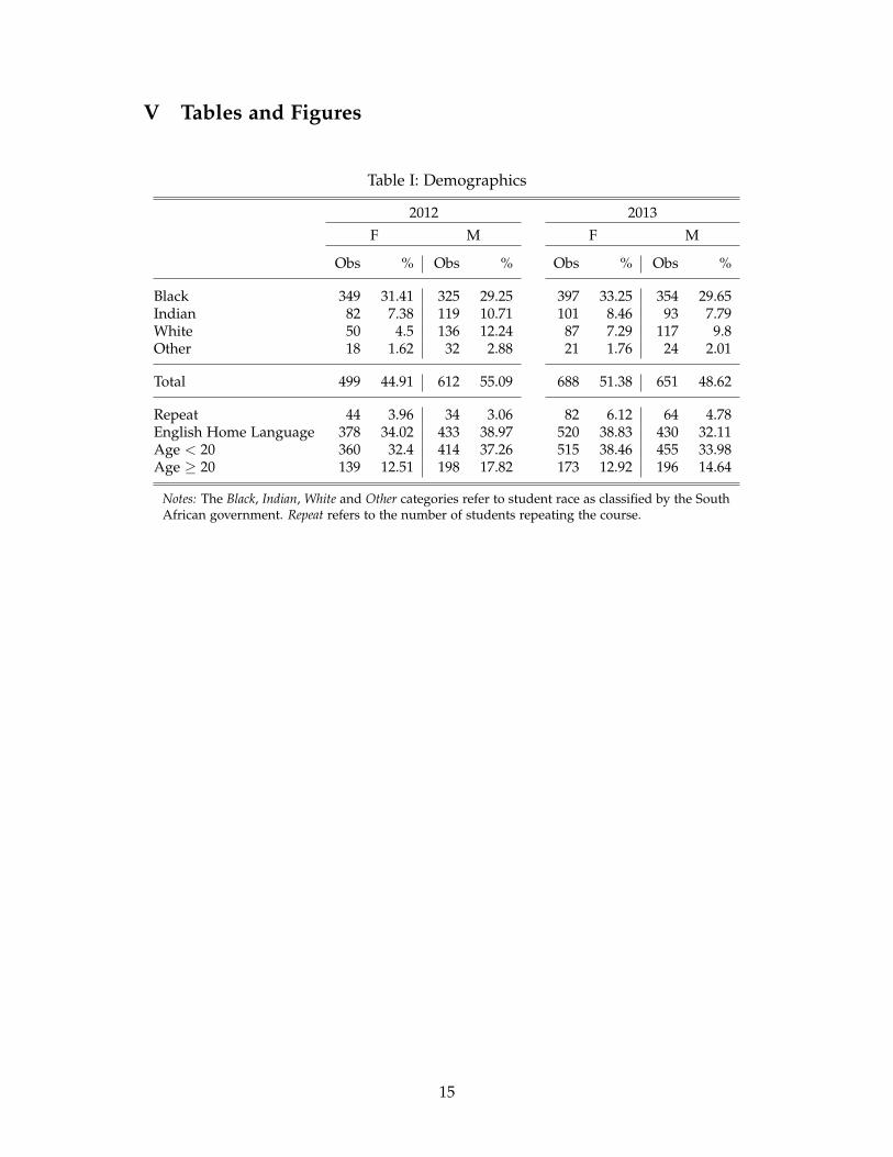
exhibit similar characteristics. Tables I and II present summary statistics for the data. The 2012

sample consists of 1111 students, 45% of whom are female. The 2013 sample consists of 1339

students, and the proportion of female students increased to 51%.

[INSERT TABLE I APPROXIMATELY HERE]

[INSERT TABLE II APPROXIMATELY HERE]

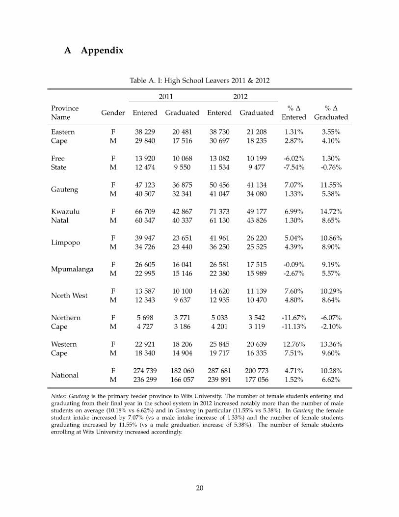
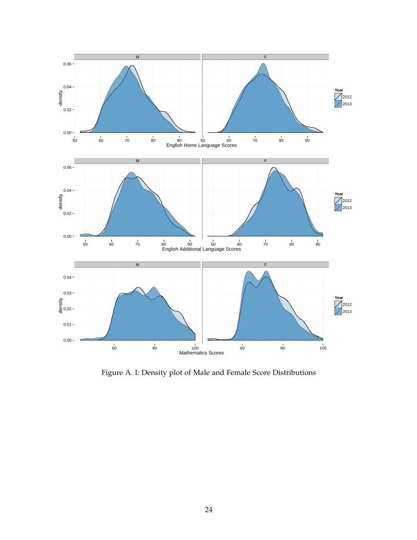
The increase in the number of students enrolled in the course is not an uncharacteristic

change, as the number of students enrolled fluctuates yearly about this range. The change in

the relative number of female students was initially a cause for concern, however, upon in-

vestigation, it simply reflects a change in the relative proportion of male and female students

initially enrolled in, and ultimately graduating from, the school system (see Table A. I). The

increase in the number of female students is therefore not expected to reflect an unobserved

group effect differentiating the relative performance of female students across the 2012 and

2013 cohorts. This is further supported by school-level academic performance statistics. Ta-

ble II shows that despite the change in gender representation, there is very little change to

students’ relative scholastic achievements.2

Although there is no clear evidence of a change in the relative scholastic abilities of male

and female students across the two cohorts, the gender-specific performance gap in Economics

scores decreased from 3.4% (2012) to 1.2% (2013). The student performance of the 2013 cohort

exhibits lower standard deviation and overall performance improved by 4.3%, with female

students improving by 5.5% and male students improving by 3.4%. Descriptive statistics there-

fore suggest that the change in assessment scoring approach had more of a positive impact

on female students than on male students. Pooled cross-section ordinary least squares (OLS)

regressions were conducted to formally assess this result, with student performance measured

by Economics MCQ assessment score as the dependent variable, and a dummy variable term

interacting gender and negative marking as the explanatory variable of interest. Student char-

acteristics generally found to correlate with gender-specific performance gaps and otherwise

influence student performance were selected as control variables to test the robustness of the

relationships. The control variables included in the robustness check were quantitative and

verbal ability, race, age, and a dummy variable for students repeating the course (Parker,

2006).

Quantile regressions were performed to further interrogate the relationship. Koenker and

Bassett (1978) introduced “regression quantiles” as a linear estimator preferable to OLS in sit-

2Figure A. I illustrates that this applies across the school-level academic performance distribution.

5

uations where there is uncertainty about the shape of the distribution generating the sample.

This applies to our data: the benefit or bias that a student accrues when negative marking is

used is implicitly dependent on the level of the student’s knowledge as well as the student’s

risk aversion. If a student knows the correct solution they will experience no benefit to a

change from negative marking to number-right scoring, because they would not have omitted

the question under the negative marking regime nor would they have been penalized for an

incorrect choice. A student with no knowledge who chooses to answer a question (a pure

guess) will achieve a 20% benefit, on average, when a number-right scoring regime is imple-

mented. The benefit accrued between these two extremes, holding risk aversion constant, is

consequently inversely proportional to a student’s knowledge. Confounding this effect, how-

ever, is that top students who are risk averse, but more likely to guess correctly (educated

guesses), stand to gain more than risk-neutral or risk-loving top students if negative mark-

ing is removed. Therefore, the coefficients of the interaction variable are not expected to be

uniform across the distribution of the assessment scores. Curiously, the literature does not

consider how the impact of negative marking may differ across the performance distribution.

Empirical studies tend to consider only the mean effect of negative marking. By using a quan-

tile regression to explore the relationship between negative marking and gender bias, we can

disaggregate the effect and reveal how it differs across the performance distribution.

The salient feature of this study is that all results were obtained in actual test sittings

and were not adjusted thereafter. The results are therefore free from the framing distortions

associated with controlled experiments. This is valuable because framing significantly affects

gender-specific risk-averse behavior (Anderson and Brown, 1984; Schubert et al., 1999; Eckel

and Grossman, 2008; Baldiga, forthcoming).

III Results

III.I Baseline Regressions

Table III shows the results of the baseline OLS and quantile regressions. The baseline OLS

model (Column 1) regresses Economics score against gender, negative marking, and their

interaction term. The results indicate a significant gender effect on Economics score, with

female students performing, on average, 1.2% worse than their male counterparts, irrespective

of whether negative marking is used. The negative marking variable is also significant and

lowers the average score for all students by 3.4%. The coefficient on the interaction term

6

is significant and supports the gender bias hypothesis indicating that, on average, female

students’ assessment scores decrease by an additional 2.2% more than their male counterparts

under a negative marking regime.

[INSERT TABLE III APPROXIMATELY HERE]

[INSERT FIGURE I APPROXIMATELY HERE]

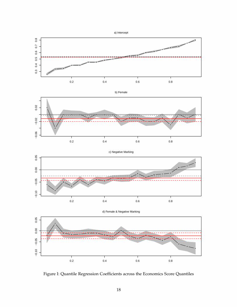
Columns 2 to 5 present the results of the quantile regressions, and Figure I illustrates these

results, graphically displaying the non-uniform distribution of the covariates’ effects. The

positive co-efficient for the negative marking dummy for students above the 90th percentile is

surprising, but may have resulted from students believing that there is less incentive to study

for assessments when number-right scoring is used3. Alternatively, it is possible that the 2013

assessments were marginally more difficult than the 2012 assessments, thereby offsetting the

gains from number-right scoring. As a third possibility, the top performers in the 2013 cohort

may have been marginally academically weaker than the 2012 cohort. Because the negative

marking dummy captures any potential year effects it is not clear what explanation plays a

significant role in determining the value of the positive coefficient.

The coefficients on the interaction dummy in Table III and illustrated in Figure I(d) provide

the crucial results. In the lower quantiles, the effect of a negative marking regime on female

students in relation to male students is small (-1.5% and -2% in the 25th and 50th percentiles,

respectively) and is not statistically significantly different from zero. At this level a lack of

knowledge appears to outweigh any significant disadvantage due to risk aversion. In the

upper quantiles, the effect is far larger (-4.3% and -7.5% for the 75th and 90th percentiles, re-

spectively) and is significant at the 1% level. These results suggest that the group of students

who benefited most from discontinuing negative marking were top performing female stu-

dents. This supports the hypothesis that top female students who are uncertain of a solution,

but are capable of correctly making an educated guess, are less likely to answer a question

under a negative marking regime than their male counterparts. Therefore, a negative mark-

ing regime significantly disadvantages the top female students. Figure II illustrates the effect

of this risk aversion on the distribution of marks. Under a negative marking regime Figure

II(a), the large distribution gap between the kernel density plots indicates that substantially

more male students received marks greater than 75% than female students. Once negative

marking is removed Figure II(b), the upper part of the distribution shows a greatly reduced

3We showed these regression results to the 2013 cohort and asked them what they thought could explain this result.They specifically stated that without negative marking they were less incentivized to study as diligently, compared tothe effort they felt compelled to commit to courses that used negative marking.

7

gap between the number of male and female students receiving marks above 75%. This shift

in distributional composition supports the regression results, indicating that female students

at the top end of the score distribution are more adversely affected by negative marking than

their male counterparts. With number-right scoring there are fewer students with scores below

25%, as expected.4

[INSERT FIGURE II APPROXIMATELY HERE]

III.II Robustness checks

The baseline regressions presented in Table III include only the gender dummy, the negative

marking dummy, and their interaction. The extended OLS and quantile regression results

presented in Table A. II serve as a robustness check of the initial result, fitting the model with

additional control variables to capture potential group effects between the two sample years.

In the extended OLS model (column 1), after controlling for differences in mathematical and

verbal ability as well as other potential explanatory factors, the gender effect is still negative,

but is no longer significant. The coefficient on the negative marking dummy is still significant

and has increased in negative magnitude, while the Mathematics and English score variables

are positive and significant. These results are congruent with the literature exploring the deter-

minants of academic performance in undergraduate Economics courses. Most notably, despite

including these control variables, the coefficient on the female and negative marking inter-

action term remains essentially unchanged and is still statistically significant at the 1% level,

indicating the robustness of this result. The extended quantile regression results (Columns

2 to 5), however, indicate that the increasingly negative interaction effect across the perfor-

mance distribution does not appear to be robust to the introduction of the additional control

covariates. Instead, the coefficient on the female and negative marking interaction term is

fairly constant (within one standard deviation) across the quantiles. Rather than undermining

the previous findings, these results illuminate a collinearity problem that arises when includ-

ing both gender and Mathematics score, or gender and English score, in the regressions. This

collinearity issue was recognized as early as Ferber et al. (1983). Tables A. III and A. IV expand

on this result.

The salient effects in Table A. III are captured by the negative marking and Mathematics

score interaction variable, and the negative marking and English interaction variables. A priori,

we would not expect a change in assessment scoring approach to change the effect of high

4With number-right scoring there is no correction for guessing. The demonstrated knowledge of the poorest per-forming students is therefore likely to be inflated due to guessed solutions.

8

school Mathematics and English ability on student Economics scores. Yet the coefficient of the

Neg Mark & Math Score variable is positive, implying that a student’s high school Mathematics

score has a larger effect on Economics scores under a negative marking regime and, in the

top quantile (Column 5), the negative Neg Mark & English Adv coefficient implies that English

ability has less of an effect under a negative marking regime. Table A. IV shows that strong

Mathematics scores are negatively correlated with the likelihood that a randomly selected

student is female, while being a strong English student is highly positively correlated with the

probability of being a female student. Together, these two results suggest that characteristics

associated with female students (i.e., weaker Mathematics ability and stronger English ability)

are negatively correlated with performance when negative marking is used. This result is

anomalous from a theoretical perspective, unless these variables are highly correlated with

another explanatory variable, such as gender. Thus, it is far more likely that the large negative

effect on top performing female students that was observed in the baseline regression is now

spuriously captured by the Mathematics and English variables. In other words, the negative

effect of being female is now erroneously captured by those characteristics that are associated

with being female. The baseline quantile regressions presented in Table III are therefore likely

to be the most appropriate measure of the treatment effect.

Three potential confounding factors which we address are that the effect: (i) is driven by

unobserved differences in a particular assessment; (ii) captures an unobserved institutional

learning effect acquired during the 2013 semester; or (iii) is driven by additional unobserved

characteristics in the 2013 female cohort, such as higher motivation or ability. To address the

first two concerns, we separately regressed the Economics score of each individual assessment

taken throughout the semester on the covariates. A large, consistent, significant, negative

coefficient on the female and negative marking interaction term was observed in the upper

quantiles of each individual assessment throughout the semester (Table A. V). The female bias

effect therefore does not appear to be driven by a particular assessment and does not appear

to have accrued during the semester due to an acquired change in behavior. To address the

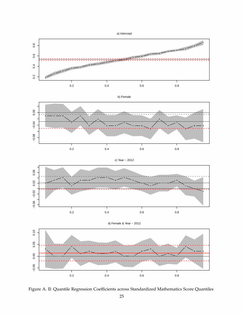
third concern, we substituted the Economics assessment scores of the regression equations for

the assessment score achieved in a first year university Mathematics course, which most Eco-

nomics students in the 2012 and 2013 cohorts had to complete. The Mathematics assessment

was a standardized assessment that used negative marking in 2013, in 2012, and in previous

years. The regression results using the Mathematics assessment scores, crucially, showed no

significant change in the gender-specific performance differential on average, or across the

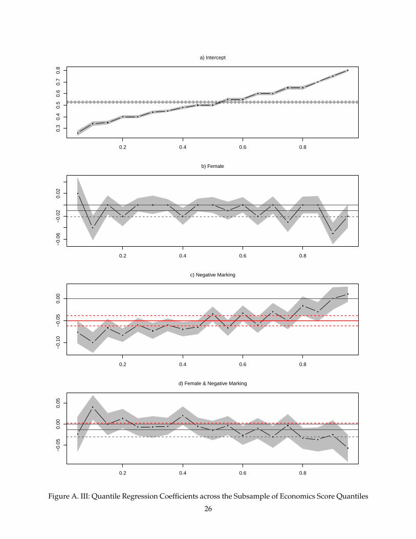
performance distribution (Figure A. II). We then limited the Economics score regressions to

9

include only the results of those students who had completed the Mathematics assessment to

ensure that the observed female bias effect was not driven by a different subsample of students

to those who had completed the Mathematics course. The regression results for the limited

sample of Economics students once again showed the same trend in increasing performance

bias for top female students (Figure A. III), although the trend was less pronounced. These

results support the conclusion that the performance effect seen in the Economics score is as a

result of the change in assessment scoring regime and is unlikely to be the result of unobserved

characteristics.

IV Implications and Concluding Remarks

While the use of negative marking is correctly motivated by the desire to further enhance the

reliability of an assessment, the possibility that negative marking may discriminate against

students according to demographic characteristics is alarming. Our results raise important

normative questions for assessment bodies deciding how best to score assessments. The dis-

tributional shift in scores in the lower quantiles when negative marking is removed clearly il-

lustrates the benefit of random guessing accrued to weaker students. The effect of the change

is to “squash” the score distribution against the 100% upper bound, confounding the dif-

ferentiation of an average student from a weak student. On the other hand, the change to

number-right scoring has a large positive effect on female students in the upper quantiles,

which is probably caused by the reduced bias effect.

There is, therefore, an unfortunate tradeoff between identifying weaker students and im-

posing a bias against the performance of top female students. Passing students due to the

random guessing effect associated with number-right scoring can negatively impact the per-

ceived quality of the course and push through weaker students; but disadvantaging strong

female students by using negative marking may result in them losing bursary and further

study opportunities. This bias may also limit opportunities for, and discriminate against, fe-

male students taking other high stakes assessments such as the SAT, potentially precipitating

future labour market disparities. However, further studies should be conducted to assess the

generalizability of our result.

The desired outcomes of a course should inform the selection of an appropriate scoring

mechanism: if a student’s ability to act in a risk neutral manner is a desirable course outcome,

then negative marking may be an appropriate assessment tool because relative risk aversion

plays a role in the student’s final score. However, this outcome is unlikely to be appropriate

10

for a course such as a first year undergraduate Economics course. If the primary desired

outcome is to assess student knowledge, then number-right scoring with an alternate screening

mechanism (such as a higher passing grade) is likely to be more desirable. Alternatively,

number-right scoring using ‘curve grading’ may be possible in large classes. In these instances,

the use of number-right scoring serves to reduce the negative female bias effect associated with

using MCQs.

School of Economic and Business Sciences, Wits University

School of Economic and Business Sciences, Wits University

11

References

Anderson, G and R Iain F Brown (1984) “Real and Laboratory Gambling, Sensation-seeking

and Arousal,” British Journal of Psychology, Vol. 75, pp. 401–410.

Archer, John (1996) “Sex Differences in Social Behavior. Are the Social Role and Evolutionary

Explanations Compatible?,” American Psychologist, Vol. 51, pp. 909–917.

Baldiga, Katherine A (forthcoming) “Gender Differences in Willingness to Guess,” Management

Science.

Becker, William E and Carol Johnston (1999) “The Relationship between Multiple Choice and

Essay Response Questions in Assessing Economics Understanding,” The Economic Record,

Vol. 75, pp. 348–357.

Ben-Shakhar, Gershon and Yakov Sinai (1991) “Gender Differences in Multiple-Choice Tests:

The Role of Differential Guessing Tendencies,” Journal of Educational Measurement, Vol. 28,

pp. 23–35.

Bliss, Leonard B (1980) “A Test of Lord’s Assumption regarding Examinee Guessing Behavior

on Multiple-Choice Tests Using Elementary School Students,” Journal of Educational Measure-

ment, Vol. 17, pp. 147–153.

Bolch, Ben W and Rendigs Fels (1974) “A note on sex and economic education,” The Journal of

Economic Education, Vol. 6, pp. 64–67.

Bridgeman, Brent and Charles Lewis (1994) “The relationship of essay and multiple-choice

scores with grades in college courses,” Journal of Educational Measurement, Vol. 31, pp. 37–50.

Buckles, Stephen and John J. Siegfried (2006) “Using Multiple-Choice Questions to Evaluate

In-Depth Learning of Economics,” The Journal of Economic Education, Vol. 37, pp. 48–57.

Burns, Justine, Simon Halliday, and Malcolm Keswell (2012) “Gender and Risk Taking in the

Classroom,” Working Paper 87, Southern Africa Labour and Development Research Unit.

Burton, Richard F (2010) “Multiple-Choice and True/False Tests: Myths and Misapprehen-

sions,” Assessment & Evaluation in Higher Education, Vol. 30, pp. 65–72.

Byrnes, James P., David C. Miller, and William D. Schafer (1999) “Gender Differences in Risk

Taking: A Meta-Analysis.,” Psychological Bulletin, Vol. 125, pp. 367–383.

12

Croson, Rachel and Uri Gneezy (2009) “Gender Differences in Preferences,” Journal of Economic

Literature, Vol. 47, pp. 448–474.

Davies, Peter, Jean Mangan, and Shqiponja Telhaj (2005) “Bold, Reckless and Adaptable? Ex-

plaining Gender Differences in Economic Thinking and Attitudes,” British Educational Re-

search Journal, Vol. 31, pp. 29–48.

Eagly, Alice H (1987) Sex Differences in Social Behavior: A Social-role Interpretation: Lawrence

Erlbaum Associates, Inc.

Eagly, Alice H and Wendy Wood (1999) “The Origins of Sex Differences in Human Behavior,”

American Psychologist, Vol. 54, pp. 408–423.

Eckel, Catherine C. and Philip J. Grossman (2008) “Forecasting Risk Attitudes: An Experi-

mental Study Using Actual and Forecast Gamble Choices,” Journal of Economic Behavior &

Organization, Vol. 68, pp. 1–17.

Espinosa, María Paz and Javier Gardeazabal (2010) “Optimal Correction for Guessing in

Multiple-Choice Tests,” Journal of Mathematical Psychology, Vol. 54, pp. 415–425.

Ferber, Marianne A, Bonnie G Birnbaum, and Carole A Green (1983) “Gender Differences in

Economic Knowledge: A Reevaluation of the Evidence,” The Journal of Economic Education,

Vol. 14, pp. 24–37.

Fisman, Raymond, Sheena S Iyengar, Emir Kamenica, and Itamar Simonson (2006) “Gender

Differences in Mate Selection: Evidence from a Speed Dating Experiment,” The Quarterly

Journal of Economics, Vol. 121, pp. 673–697.

Gaulin, Steven and Harol Hoffman (1988) “Evolution and Development of Sex Differences in

Spatial Ability,” in Laura Betzig, Monique Borgerhoff Mulder, and Paul Turke eds. Human

Reproductive Behavior: A Darwinian Perspective: Cambridge University Press, Chap. 7.

Geary, David C (2009) Male, Female: The Evolution of Human Sex Differences.: American Psycho-

logical Association, 2nd edition.

Gneezy, Uri., Muriel. Niederle, and Aldo. Rustichini (2003) “Performance in Competitive En-

vironments: Gender Differences,” The Quarterly Journal of Economics, Vol. 118, pp. 1049–1074.

Holt, Alan (2006) “An analysis of negative marking in multiple-choice assessment,” in Proceed-

ings of 19th Annual Conference of the National Advisory Committee on Computing Qualifications,

pp. 115–118.

13

Kelly, Shona and Reg Dennick (2009) “Evidence of Gender Bias in True-False-Abstain Medical

Examinations.,” BMC medical education, Vol. 9.

Koenker, Roger and Gilbert Jr Bassett (1978) “Regression quantiles,” Econometrica, Vol. 46, pp.

33–50.

Maccoby, Eleanor Emmons and Carol Nagy Jacklin (1974) The Psychology of Sex Differences:

Stanford University Press.

Marín, C and A Rosa-García (2011) “Gender Bias in Risk Aversion: Evidence from Multiple

Choice Exams,” Working Paper 39987, MPRA.

McHarg, Jane, Paul Bradley, Suzanne Chamberlain, Chris Ricketts, Judy Searle, and John C

McLachlan (2005) “Assessment of Progress Tests.,” Medical Education, Vol. 39, pp. 221–227,

DOI: http://dx.doi.org/10.1111/j.1365-2929.2004.02060.x.

Moss, Edward (2001) “Multiple Choice Questions: Their Value as an Assessment Tool.,” Cur-

rent Opinion in Anesthesiology, Vol. 14, pp. 661–6.

Niederle, Muriel and Lise Vesterlund (2010) “Explaining The Gender Gap in Math Test Scores:

The Role of Competition,” The Journal of Economic Perspectives, Vol. 24, pp. 129–144.

Parker, Kudayja (2006) “The Effect of Student Characteristics on Achievement in Introductory

Microeconomics in South Africa,” South African Journal of Economics, Vol. 74, pp. 137–149.

Schubert, Renate, Martin Brown, Matthias Gysler, and Hans Wolfgang Brachinger (1999) “Fi-

nancial Decision-Making: Are Women Really More Risk-Averse?” The American Economic

Review, Vol. 89, pp. 381–385, URL: http://www.jstor.org/stable/117140.

Siegfried, John J (1979) “Male-female Differences in Economic Education: A Survey,” The Jour-

nal of Economic Education, Vol. 10, pp. 1–11, URL: http://www.jstor.org/stable/1182372.

Simkin, Mark G and William L Kuechler (2005) “Multiple-Choice Tests and Student Under-

standing: What is the Connection?” Decision Sciences Journal of Innovative Education, Vol. 3,

pp. 73–97.

Walstad, William B and William E Becker (1994) “Achievement Differences on Multiple-Choice

and Essay Tests in Economics,” The American Economic Review, Vol. 84, pp. 193–196.

Walstad, William B and Phillip Saunders (1998) Teaching Undergraduate Economics: A Handbook

for Instructors: McGraw-Hill/Irwin, 1st edition.

14

V Tables and Figures

Table I: Demographics

2012 2013

F M F M

Obs % Obs % Obs % Obs %

Black 349 31.41 325 29.25 397 33.25 354 29.65Indian 82 7.38 119 10.71 101 8.46 93 7.79White 50 4.5 136 12.24 87 7.29 117 9.8Other 18 1.62 32 2.88 21 1.76 24 2.01

Total 499 44.91 612 55.09 688 51.38 651 48.62

Repeat 44 3.96 34 3.06 82 6.12 64 4.78English Home Language 378 34.02 433 38.97 520 38.83 430 32.11Age < 20 360 32.4 414 37.26 515 38.46 455 33.98Age ≥ 20 139 12.51 198 17.82 173 12.92 196 14.64

Notes: The Black, Indian, White and Other categories refer to student race as classified by the SouthAfrican government. Repeat refers to the number of students repeating the course.

15

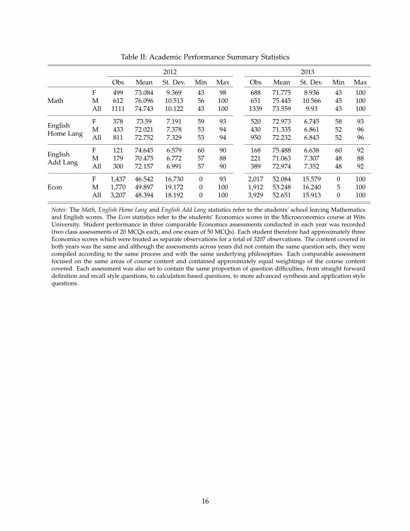
Table II: Academic Performance Summary Statistics

2012 2013

Obs Mean St. Dev. Min Max Obs Mean St. Dev. Min Max

MathF 499 73.084 9.369 43 98 688 71.775 8.936 43 100M 612 76.096 10.513 56 100 651 75.445 10.566 45 100All 1111 74.743 10.122 43 100 1339 73.559 9.93 43 100

EnglishHome Lang

F 378 73.59 7.191 59 93 520 72.973 6.745 58 93M 433 72.021 7.378 53 94 430 71.335 6.861 52 96All 811 72.752 7.329 53 94 950 72.232 6.843 52 96

EnglishAdd Lang

F 121 74.645 6.579 60 90 168 75.488 6.638 60 92M 179 70.475 6.772 57 88 221 71.063 7.307 48 88All 300 72.157 6.991 57 90 389 72.974 7.352 48 92

EconF 1,437 46.542 16.730 0 93 2,017 52.084 15.579 0 100M 1,770 49.897 19.172 0 100 1,912 53.248 16.240 5 100All 3,207 48.394 18.192 0 100 3,929 52.651 15.913 0 100

Notes: The Math, English Home Lang and English Add Lang statistics refer to the students’ school leaving Mathematicsand English scores. The Econ statistics refer to the students’ Economics scores in the Microeconomics course at WitsUniversity. Student performance in three comparable Economics assessments conducted in each year was recorded(two class assessments of 20 MCQs each, and one exam of 50 MCQs). Each student therefore had approximately threeEconomics scores which were treated as separate observations for a total of 3207 observations. The content covered inboth years was the same and although the assessments across years did not contain the same question sets, they werecompiled according to the same process and with the same underlying philosophies. Each comparable assessmentfocused on the same areas of course content and contained approximately equal weightings of the course contentcovered. Each assessment was also set to contain the same proportion of question difficulties, from straight forwarddefinition and recall style questions, to calculation based questions, to more advanced synthesis and application stylequestions.

16

Table III: Baseline Regression Results

Dependent variable: Economics Score

OLS Quantile regressions25th 50th 75th 90th

(1) (2) (3) (4) (5)

Female −0.012∗∗ 0.000 −0.020∗∗ −0.010 −0.010(0.005) (0.006) (0.008) (0.007) (0.009)

Neg Mark −0.034∗∗∗ −0.040∗∗∗ −0.035∗∗∗ −0.017∗∗ 0.017∗∗

(0.006) (0.008) (0.008) (0.008) (0.007)

Female & Neg Mark −0.022∗∗∗ −0.015 0.002 −0.043∗∗∗ −0.072∗∗∗

(0.008) (0.011) (0.011) (0.012) (0.013)

Constant 0.532∗∗∗ 0.400∗∗∗ 0.520∗∗∗ 0.650∗∗∗ 0.750∗∗∗

(0.004) (0.006) (0.006) (0.003) (0.002)

Observations 7,136 7,136 7,136 7,136 7,136

Notes: Female dummy = 1 for female students; Neg Mark dummy = 1 for assessments in whichnegative marking was used (i.e.: 2012); Female & Neg Mark is the Female and Neg Mark interactionterm of interest. ∗p<0.1; ∗∗p<0.05; ∗∗∗p<0.01

17

0.2 0.4 0.6 0.8

0.3

0.4

0.5

0.6

0.7

0.8

a) Intercept

0.2 0.4 0.6 0.8

−0.

06−

0.02

0.02

b) Female

0.2 0.4 0.6 0.8

−0.

10−

0.05

0.00

0.05

c) Negative Marking

0.2 0.4 0.6 0.8

−0.

10−

0.05

0.00

0.05

d) Female & Negative Marking

Figure I: Quantile Regression Coefficients across the Economics Score Quantiles

18

a) Negative Marking b) Number Right Scoring

0.0

0.5

1.0

1.5

2.0

2.5

0.00 0.25 0.50 0.75 1.00 0.00 0.25 0.50 0.75 1.00score

dens

ity

Sex

M

F

Figure II: Density plot of Male and Female Economics Score Distributions

19

A Appendix

Table A. I: High School Leavers 2011 & 2012

2011 2012

ProvinceName

Gender Entered Graduated Entered Graduated% ∆

Entered% ∆

Graduated

EasternCape

F 38 229 20 481 38 730 21 208 1.31% 3.55%M 29 840 17 516 30 697 18 235 2.87% 4.10%

FreeState

F 13 920 10 068 13 082 10 199 -6.02% 1.30%M 12 474 9 550 11 534 9 477 -7.54% -0.76%

GautengF 47 123 36 875 50 456 41 134 7.07% 11.55%M 40 507 32 341 41 047 34 080 1.33% 5.38%

KwazuluNatal

F 66 709 42 867 71 373 49 177 6.99% 14.72%M 60 347 40 337 61 130 43 826 1.30% 8.65%

LimpopoF 39 947 23 651 41 961 26 220 5.04% 10.86%M 34 726 23 440 36 250 25 525 4.39% 8.90%

MpumalangaF 26 605 16 041 26 581 17 515 -0.09% 9.19%M 22 995 15 146 22 380 15 989 -2.67% 5.57%

North WestF 13 587 10 100 14 620 11 139 7.60% 10.29%M 12 343 9 637 12 935 10 470 4.80% 8.64%

NorthernCape

F 5 698 3 771 5 033 3 542 -11.67% -6.07%M 4 727 3 186 4 201 3 119 -11.13% -2.10%

WesternCape

F 22 921 18 206 25 845 20 639 12.76% 13.36%M 18 340 14 904 19 717 16 335 7.51% 9.60%

NationalF 274 739 182 060 287 681 200 773 4.71% 10.28%M 236 299 166 057 239 891 177 056 1.52% 6.62%

Notes: Gauteng is the primary feeder province to Wits University. The number of female students entering andgraduating from their final year in the school system in 2012 increased notably more than the number of malestudents on average (10.18% vs 6.62%) and in Gauteng in particular (11.55% vs 5.38%). In Gauteng the femalestudent intake increased by 7.07% (vs a male intake increase of 1.33%) and the number of female studentsgraduating increased by 11.55% (vs a male graduation increase of 5.38%). The number of female studentsenrolling at Wits University increased accordingly.

20

Table A. II: Extended Regression Results

Dependent variable: Economics Score

OLS Quantile Regressions

25th 50th 75th 90th(1) (2) (3) (4) (5)

Female −0.006 0.0004 −0.007 −0.020∗∗∗ −0.016∗∗

(0.005) (0.007) (0.006) (0.006) (0.008)

Neg Mark −0.041∗∗∗ −0.052∗∗∗ −0.041∗∗∗ −0.037∗∗∗ −0.023∗∗∗

(0.005) (0.007) (0.007) (0.007) (0.008)

Female & Neg Mark −0.023∗∗∗ −0.020∗∗ −0.023∗∗ −0.017∗ −0.022∗

(0.007) (0.010) (0.009) (0.010) (0.012)

Math Score 0.006∗∗∗ 0.006∗∗∗ 0.007∗∗∗ 0.007∗∗∗ 0.007∗∗∗

(0.0002) (0.0003) (0.0002) (0.0003) (0.0003)

English Score 0.003∗∗∗ 0.003∗∗∗ 0.002∗∗∗ 0.003∗∗∗ 0.003∗∗∗

(0.0005) (0.001) (0.001) (0.001) (0.001)

English −0.010 −0.021∗∗ −0.012 0.005 0.008(0.007) (0.011) (0.009) (0.009) (0.012)

English Adv −0.034 −0.044 −0.117∗∗ 0.011 0.088(0.041) (0.060) (0.049) (0.055) (0.068)

Eng Adv & Eng Score 0.001∗∗∗ 0.002∗ 0.003∗∗∗ 0.001 −0.0003(0.001) (0.001) (0.001) (0.001) (0.001)

Constant −0.197∗∗∗ −0.263∗∗∗ −0.193∗∗∗ −0.260∗∗∗ −0.095(0.057) (0.083) (0.069) (0.079) (0.096)

Observations 7,136 7,136 7,136 7,136 7,136

Notes: All regressions are of the form: Economics Score = β0 + β1Female + β2NegMark +β3Female × NegMark + β4MathScore + β5EnglishScore + β6English + β7EnglishAdv +β8EngAdv× EngScore+ β9RepeatStudent+ β10Age+ β11−14Race+ β15−18Race× sex. Fe-male = 1 for female students. Neg Mark dummy = 1 for assessments in which negativemarking is used. Math Score and English Score refer to high school Mathematics andEnglish marks on a 0 to 100 scale. South African schools allow students to take twodifferent English courses: Home Language and Additional language. To account forthis, we include an additional dummy variable English Adv to code for those studentswho completed the more advanced Home Language course. Thus, for Home Languagestudents, the coefficients of the English Adv and Eng Adv & Eng Score variable shouldbe considered in conjunction with the English Score coefficient. The omitted covariantscontrol for any potential demographic effects but add little to the discussion and areavailable on request. ∗p<0.1; ∗∗p<0.05; ∗∗∗p<0.01

21

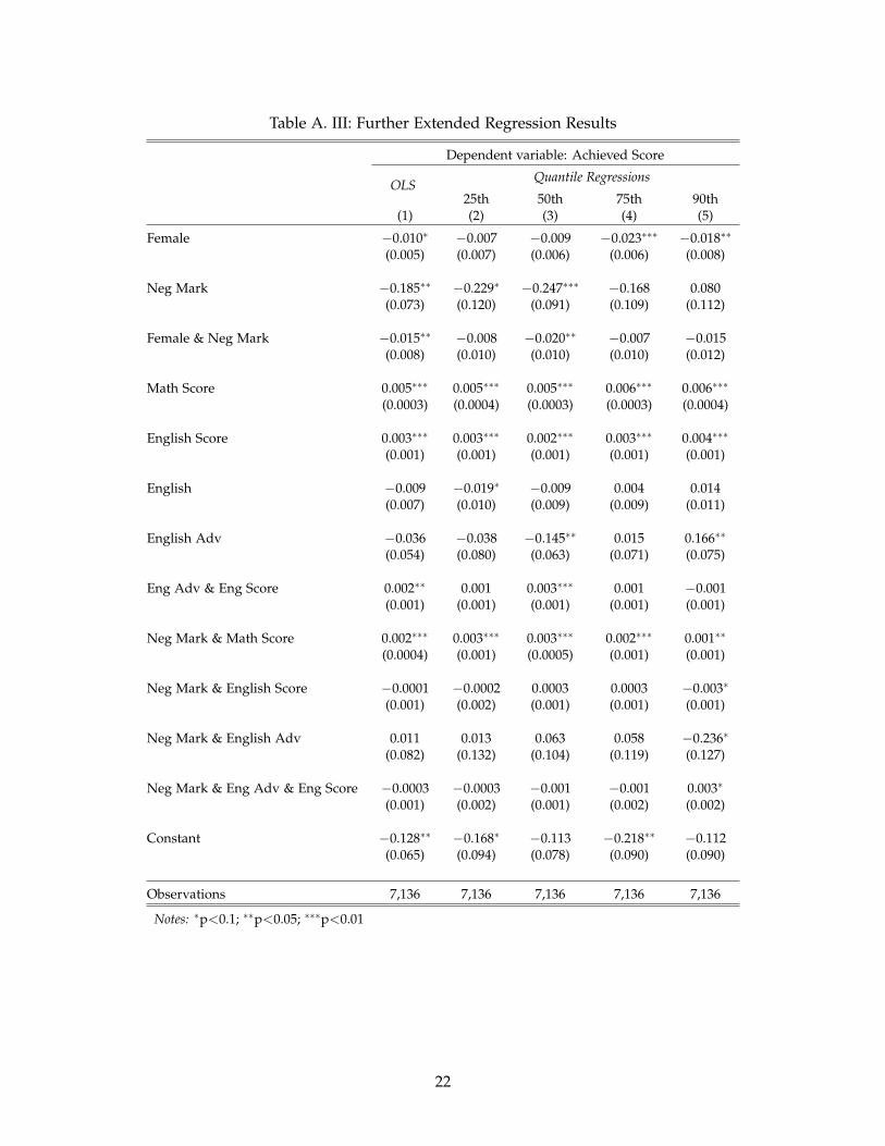
Table A. III: Further Extended Regression Results

Dependent variable: Achieved Score

OLS Quantile Regressions

25th 50th 75th 90th(1) (2) (3) (4) (5)

Female −0.010∗ −0.007 −0.009 −0.023∗∗∗ −0.018∗∗

(0.005) (0.007) (0.006) (0.006) (0.008)

Neg Mark −0.185∗∗ −0.229∗ −0.247∗∗∗ −0.168 0.080(0.073) (0.120) (0.091) (0.109) (0.112)

Female & Neg Mark −0.015∗∗ −0.008 −0.020∗∗ −0.007 −0.015(0.008) (0.010) (0.010) (0.010) (0.012)

Math Score 0.005∗∗∗ 0.005∗∗∗ 0.005∗∗∗ 0.006∗∗∗ 0.006∗∗∗

(0.0003) (0.0004) (0.0003) (0.0003) (0.0004)

English Score 0.003∗∗∗ 0.003∗∗∗ 0.002∗∗∗ 0.003∗∗∗ 0.004∗∗∗

(0.001) (0.001) (0.001) (0.001) (0.001)

English −0.009 −0.019∗ −0.009 0.004 0.014(0.007) (0.010) (0.009) (0.009) (0.011)

English Adv −0.036 −0.038 −0.145∗∗ 0.015 0.166∗∗

(0.054) (0.080) (0.063) (0.071) (0.075)

Eng Adv & Eng Score 0.002∗∗ 0.001 0.003∗∗∗ 0.001 −0.001(0.001) (0.001) (0.001) (0.001) (0.001)

Neg Mark & Math Score 0.002∗∗∗ 0.003∗∗∗ 0.003∗∗∗ 0.002∗∗∗ 0.001∗∗

(0.0004) (0.001) (0.0005) (0.001) (0.001)

Neg Mark & English Score −0.0001 −0.0002 0.0003 0.0003 −0.003∗

(0.001) (0.002) (0.001) (0.001) (0.001)

Neg Mark & English Adv 0.011 0.013 0.063 0.058 −0.236∗

(0.082) (0.132) (0.104) (0.119) (0.127)

Neg Mark & Eng Adv & Eng Score −0.0003 −0.0003 −0.001 −0.001 0.003∗

(0.001) (0.002) (0.001) (0.002) (0.002)

Constant −0.128∗∗ −0.168∗ −0.113 −0.218∗∗ −0.112(0.065) (0.094) (0.078) (0.090) (0.090)

Observations 7,136 7,136 7,136 7,136 7,136

Notes: ∗p<0.1; ∗∗p<0.05; ∗∗∗p<0.01

22

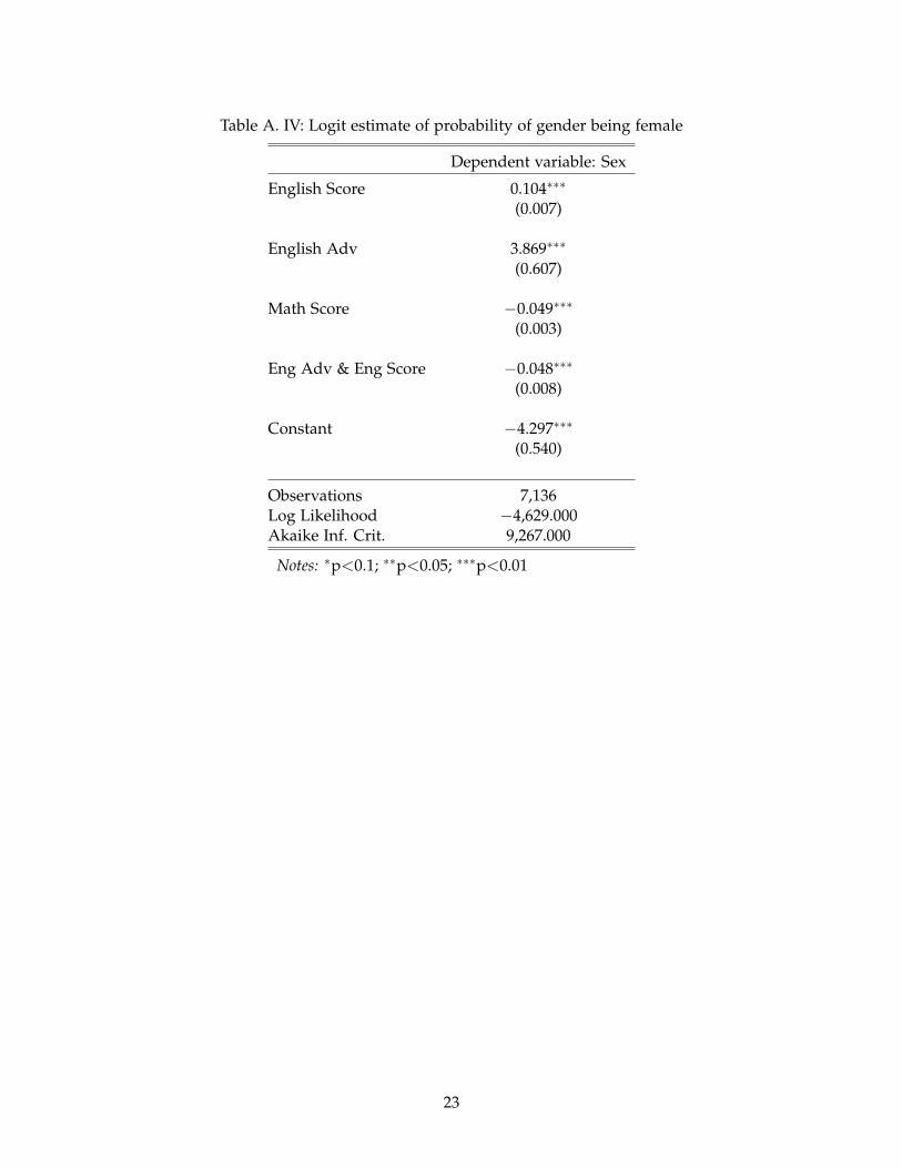
Table A. IV: Logit estimate of probability of gender being female

Dependent variable: Sex

English Score 0.104∗∗∗

(0.007)

English Adv 3.869∗∗∗

(0.607)

Math Score −0.049∗∗∗

(0.003)

Eng Adv & Eng Score −0.048∗∗∗

(0.008)

Constant −4.297∗∗∗

(0.540)

Observations 7,136Log Likelihood −4,629.000Akaike Inf. Crit. 9,267.000

Notes: ∗p<0.1; ∗∗p<0.05; ∗∗∗p<0.01

23

M F

0.00

0.02

0.04

0.06

50 60 70 80 90 50 60 70 80 90English Home Language Scores

dens

ity

Year

2012

2013

M F

0.00

0.02

0.04

0.06

50 60 70 80 90 50 60 70 80 90English Additional Language Scores

dens

ity

Year

2012

2013

M F

0.00

0.01

0.02

0.03

0.04

60 80 100 60 80 100Mathematics Scores

dens

ity

Year

2012

2013

Figure A. I: Density plot of Male and Female Score Distributions

24

0.2 0.4 0.6 0.8

0.2

0.4

0.6

0.8

a) Intercept

0.2 0.4 0.6 0.8

−0.

08−

0.04

0.00

b) Female

0.2 0.4 0.6 0.8

−0.

06−

0.02

0.02

0.06

c) Year − 2012

0.2 0.4 0.6 0.8

−0.

050.

000.

050.

10

d) Female & Year − 2012

Figure A. II: Quantile Regression Coefficients across Standardized Mathematics Score Quantiles

25

0.2 0.4 0.6 0.8

0.3

0.4

0.5

0.6

0.7

0.8

a) Intercept

0.2 0.4 0.6 0.8

−0.

06−

0.02

0.02

b) Female

0.2 0.4 0.6 0.8

−0.

10−

0.05

0.00

c) Negative Marking

0.2 0.4 0.6 0.8

−0.

050.

000.

05

d) Female & Negative Marking

Figure A. III: Quantile Regression Coefficients across the Subsample of Economics Score Quantiles

26

Table A. V: Individual Test Quantile Regression Results

25th 50th 75th 90th

Dependent variable: Test 1 Results

Female 0.000 0.000 0.000 0.000(0.019) (0.015) (0.012) (0.016)

Neg Mark −0.083∗∗∗ −0.050∗∗∗ −0.033∗∗∗ 0.000(0.021) (0.014) (0.012) (0.020)

Female & Neg Mark 0.000 0.000 −0.050∗∗∗ −0.067∗∗

(0.028) (0.022) (0.018) (0.029)

Constant 0.450∗∗∗ 0.550∗∗∗ 0.700∗∗∗ 0.800∗∗∗

(0.017) (0.007) (0.008) (0.011)

Observations 2,419 2,419 2,419 2,419

Dependent variable: Test 2 Results

Female −0.050∗∗∗ −0.050∗∗∗ −0.050∗∗∗ −0.050∗∗∗

(0.012) (0.010) (0.019) (0.016)

Neg Mark −0.030∗∗ −0.010 0.030 0.060∗∗∗

(0.012) (0.012) (0.019) (0.020)

Female & Neg Mark 0.020 0.010 −0.020 −0.050∗∗

(0.019) (0.017) (0.023) (0.025)

Constant 0.400∗∗∗ 0.500∗∗∗ 0.600∗∗∗ 0.700∗∗∗

(0.009) (0.007) (0.017) (0.012)

Observations 2,365 2,365 2,365 2,365

Dependent variable: Exam Results

Female 0.000 0.000 0.000 0.000(0.009) (0.011) (0.014) (0.019)

Neg Mark −0.065∗∗∗ −0.050∗∗∗ −0.005 0.010(0.012) (0.014) (0.016) (0.018)

Female & Neg Mark −0.025 −0.030 −0.065∗∗∗ −0.055∗∗

(0.016) (0.019) (0.023) (0.024)

Constant 0.420∗∗∗ 0.520∗∗∗ 0.620∗∗∗ 0.720∗∗∗

(0.007) (0.008) (0.010) (0.014)

Observations 2,352 2,352 2,352 2,352

Note: All tests compared to corresponding tests in the previous year,i.e. Test 1-2012 (which used Negative Marking) to Test 1-2013 (whichdid not). The zero coefficients of the Female variable in the Exam andTest 1 reflect the fact the median male and female marks were the same.This is unsurprising given the small discreet space of potential scoresin an individual assessment. ∗p<0.1; ∗∗p<0.05; ∗∗∗p<0.01

27