Who Bears the Cost of a Change in theExchange Rate? The Case of Imported Beer∗

Rebecca HellersteinInternational Research FunctionFederal Reserve Bank of New York

January 2004

Abstract

Nominal exchange rates are remarkably volatile. They ordinarily appear disconnected from thefundamentals of the economies whose currencies they price. These facts make up a classic puzzleabout the international economy. If prices do not respond fully to changes in the nominal exchangerate, who bears the cost of such large and unpredictable changes: foreign firms, domestic firms, ordomestic consumers? This study develops a structural approach to analyze the welfare effects of achange in the nominal exchange rate using the example of the beer market. I estimate a structuraleconometric model that makes it possible to compute manufacturers’ and retailers’ pass-throughof a nominal exchange-rate change without observing wholesale prices or firms’ marginal costs.I conduct counterfactual experiments to quantify how the change affects domestic and foreignfirms’ profits and domestic consumer welfare. The counterfactual experiments show that foreignmanufacturers bear more of the cost of a change in the nominal exchange rate than do domesticconsumers, domestic manufacturers, or the domestic retailer. Following a 10-percent domestic-currency depreciation, foreign manufacturers’ profits decline by 22 percent, domestic consumersurplus falls by 8 percent, the retailer’s profits fall by 5 percent, and domestic manufacturers’profits increase by 1.7 percent. The model can be applied to other industries and can serve as atool to assess the welfare effects of various exchange-rate policies.

Keywords: exchange-rate pass-through, cross-border vertical contracts, welfare effects ofexchange-rate fluctuations.

JEL Classification: F31, F41, F42..

∗I am indebted to my advisors Maury Obstfeld and Aviv Nevo for valuable comments and suggestions. I alsothank George Akerlof, Severin Borenstein, Richard Gilbert, Paola Giuliano, Dan McFadden, Sofia Berto Villas-Boas,and Catherine Wolfram for their comments. I gratefully acknowledge financial support from a U.C. Berkeley Dean’sFellowship. Address: International Research, Federal Reserve Bank of New York, 33 Liberty Street, New York, NY,10045; email: Rebecca.Hellerstein@ny.frb.org.

1 Introduction

Nominal exchange rates are remarkably volatile. They ordinarily appear

disconnected from the fundamentals of the economies whose currencies they

price. These facts make up a classic puzzle about the international econ-

omy. If prices do not respond fully to changes in the nominal exchange rate,

who bears the cost of such large and unpredictable changes: foreign �rms,

domestic �rms, or domestic consumers? This study examines the welfare ef-

fects of a change in the nominal exchange rate using the example of the beer

industry. We should care about analyzing these welfare e¤ects, not only to

understand how the nominal exchange rate a¤ects the domestic economy but

also because assumptions about exchange-rates�welfare e¤ects shape econo-

mists�policy recommendations on basic issues in international �nancial mar-

kets. For example, policymakers often want to know how much a currency

must depreciate to eliminate a given trade de�cit. How �rms choose to pass

through an exchange-rate depreciation determines the depreciation�s welfare

e¤ects, including its e¤ect on the trade balance. Exchange-rate pass-through

is conventionally de�ned as the percent change in an imported good�s local-

currency price for a given percent change in the nominal exchange rate.

More empirical evidence about �rms�pass-through behavior would enable

economists to recommend a welfare-maximizing response to a given trade

1

de�cit. Such evidence would also shape policy recommendations on such is-

sues as the choice of exchange-rate regime, the conduct of monetary policy,

and the response to a currency crisis.

I develop and estimate a structural econometric model that o¤ers pre-

dictions linking �rms�pass-through behavior to strategic interactions with

other �rms (supply conditions) and to interactions with consumers (demand

conditions). Using the estimated demand system, I conduct counterfactual

experiments to quantify how a nominal exchange-rate change a¤ects domes-

tic and foreign �rms�pro�ts and consumer surplus. The structural model

computes these e¤ects without observing wholesale prices or marginal costs

(of manufacturers or retailers). The model can be applied to other industries

and can serve as a tool to assess the welfare e¤ects of various exchange-rate

policies.

My general strategy is to estimate brand-level demand and then to use

those estimates jointly with assumptions about �rms�pricing behavior to re-

cover both retail and manufacturer marginal costs without observing actual

costs. I then use the estimated demand system, assumptions about �rms�

pricing behavior, and the derived marginal costs to compute the new equilib-

rium following an exchange-rate-induced change in foreign brands�marginal

costs. I compute the change in �rms�pro�ts and in consumer surplus using

2

the new equilibrium prices and quantities.

The model�s key identi�cation assumption is that nominal exchange-

rate �uctuations dwarf other shocks to manufacturers�marginal costs such

as productivity or input-price changes over the short term. Figure 1 shows

that the exchange rate is much more volatile than are brewers�other typical

marginal costs. Thus this assumption, though strong, has clear support in

the data. The paper presents �gures that indicate the model appears to

captures exchange-rate movements for each of the sample�s countries.

Figure 1: The nominal exchange rate �uctuates by much more than do othertypical input prices for German brewers.

Though several theoretical papers examine how exchange-rate �uctua-

3

tions may a¤ect welfare, no published empirical study has formally esti-

mated these costs.1 A valuable antecedent of this paper is Kadiyali�s (1997)

structural model of pass-through in the �lm industry. Kadiyali�s model is

applicable, however, only to industries with very few products, while the

model presented here can be applied to many industries.2

I empirically test for the best-�t vertical market structure in the beer

market in another paper by comparing accounting price-cost margins to

the derived price-cost margins each vertical model produces and by using

non-nested tests developed by Villas-Boas (2003). This paper�s empirical

analysis focuses on the best-�t vertical market structure for this industry,

that is, double marginalization with manufacturers acting as multi-product

�rms.3

My data come from a single large retailer (with 120 stores) in a major

Midwestern city. I use a panel data set of retail prices and quantities sold

for 34 products from a number of manufacturers over 40 months (July 1991-

December 1994). My model thus includes a single retailer and a number

of manufacturers, whom I model as Bertrand-Nash competitors with di¤er-

1Devereux, Engel, and Tille (2003) and Corsetti, Pesenti, Roubini, and Tille (2000)present theoretical models of the welfare e¤ects of exchange-rate �uctuations.

2Another important predecessor is Goldberg�s (1995) structural model of the U.S. automarket which uses a nested-logit demand system.

3For more detail on the double-marginalization supply model, see Tirole (1988).

4

entiated products. The model includes an outside good and thus does not

assume that the retailer has a monopoly in the local market.

Beer is a good that is fairly concentrated at the manufacturer level,

consistent with my assumption of oligopoly. Because manufactured goods�

prices tend to exhibit dampened responses to exchange rates in aggregate

data, beer is an appropriate choice to investigate the puzzling phenomenon

of incomplete pass-through. The threat of trade barriers such as voluntary

export restraints or antidumping sanctions that likely a¤ect price-setting

behavior in other industries, such as autos or textiles, are rare in this indus-

try.

The counterfactual experiments produce three major results. First, for-

eign manufacturers generally bear more of the cost (or reap more of the ben-

e�t) of a change in the nominal exchange rate than do consumers, domestic

manufacturers, or the retailer. Following a 10-percent domestic currency

depreciation, foreign manufacturers�pro�ts decline by 22 percent, domestic

consumer surplus by 8 percent, and the retailer�s pro�ts by 5 percent: Do-

mestic manufacturers�pro�ts increase by 1.7 percent. Second, the results

suggest some strategic interaction between domestic and foreign manufactur-

ers following a depreciation: domestic manufacturers with brands that are

close substitutes for foreign brands increase their pro�ts by lowering prices

5

to take market share from foreign manufacturers. Third, previous work on

pass-through did not model the pricing decision of the retailer, and thus

implicitly assumed that manufacturers�interactions with downstream �rms

did not matter. My �ndings suggest that the retailer plays an important role

by absorbing part of an exchange-rate-induced marginal-cost shock before it

reaches consumers. I �nd that the retailer passes through wholesale-price in-

creases on domestic brands fully, but only partially passes through identical

price increases on foreign brands. The retailer�s markups on foreign brands

are roughly three times its markups on domestic brands: the retailer may

regard these higher markups as compensation for their greater �uctuation

over time.

Incomplete data has limited the pass-through literature. Prices along the

distribution chain, particularly import and wholesale prices, are typically

unavailable. It is also di¢ cult to obtain cost data amenable to comparison

from foreign manufacturers. As a result, there is virtually no disaggregated

empirical evidence on exchange-rate pass-through.4 Most studies use price

indexes that leave their estimates vulnerable to aggregation bias. The con-

sensus in these studies is that �rms pass through, on average, 50 percent of a

4Only one paper by Kadiyali (1997) estimates pass-through coe¢ cients using product-level prices.

6

nominal exchange-rate change to import prices over the course of one year.5

This paper uses product-level transaction prices, allowing for an empirical

method based on a model of individual �rms�price-setting behavior rather

than aggregate price indexes.

The empirical method presented in this paper also o¤ers an alternative to

the standard reduced-form approach used to estimate exchange-rate pass-

through. The standard approach has the weakness of producing di¤erent

for researchers using identical data. That approach uses a speci�cation that

imposes a �rm�s markup adjustment through the choice of functional form.6

Such a model cannot gauge the extent of the strategic pricing behavior that

�rms engage in to protect their margins.

The rest of the paper proceeds as follows. In the next section, I review

the theoretical model. Section 3 discusses the market and the data, and

section 4 sets out the estimation methodology. Results from the random-

coe¢ cients demand model are reported in section 5, and the results of the

counterfactual experiments in section 6. The last section concludes.

5Goldberg and Knetter (1997).6The assumption implicit in the standard approach is that the markup adjustment is

exactly inversely proportional to the pass-through.

7

2 Model

This section describes the supply model and the random-coe¢ cients model

used to estimate demand. It then derives simple expressions to compute

exchange-rate pass-through coe¢ cients.

2.1 Supply

Consider a double-marginalization supply model in which manufacturers act

as Bertrand oligopolists with di¤erentiated products. Strategic interactions

between manufacturers and the single retailer with respect to prices follow

a sequential Nash model. Manufacturers set their prices �rst and the re-

tailer then sets its prices taking the wholesale prices it observes as given.

Thus, a double margin is added to the marginal cost to produce the product.

To solve the model, one uses backwards induction and solves the retailer�s

problem �rst. The variety of potential interactions between manufactur-

ers, retailers, and consumers makes any theoretical prediction about welfare

e¤ects contingent on fairly precise assumptions about consumer or �rm be-

havior. In this model, I consider only one retailer as the data used for the

empirical analysis have prices for only a single retail �rm.

8

2.1.1 Retailer

Consider a single retail �rm that sells all of the market�s J di¤erentiated

products. The model assumes that all �rms use linear pricing and face

constant marginal costs. The pro�ts of the retail �rm in market t are given

by:

�t =Xj

(prjt � pwjt �mcrjt)sjt(prt )� Cf (1)

where prjt is the price the retailer sets for product j , pwjt is the wholesale

price paid by the retailer for product j , mcrjt is the the retailer�s marginal

cost for product j (excluding the wholesale price of the good), sjt(pr) is

the market share of product j which is a function of the prices of all J

products, and Cf is a �xed cost of production. Assuming the retailer sets

prices to maximize pro�ts, the retail price prj must satisfy the �rst-order

pro�t-maximizing condition:

sjt +Xk

(prkt � pwkt �mcrkt)@skt@prjt

= 0; for j ; k = 1 ; 2 ; :::; J t: (2)

This gives us a set of J equations, one for each product. The markups

can be solved for by de�ning Sjk = �@skt(prt )

@prjtj; k = 1; :::; J :; and a J � J

matrix rt called the retailer reaction matrix with the j th, kth element

equal to Sjk ; the marginal change in the kth product�s market share given

9

a change in the j th product�s retail price. The stacked �rst-order conditions

can be rewritten in vector notation:

st +rt(prt � pwt �mcrt ) = 0 (3)

as can the retailer�s markup equation:

prt = pwt +mc

rt + (rt)

�1 st (4)

2.1.2 Manufacturers

Let there be M manufacturers that each produce some subset �mt of the

market�s Jt di¤erentiated products. Each manufacturer chooses its wholesale

price pwjt while assuming the retailer behaves according to its �rst-order

condition (3). The manufacturer�s pro�t function is:

�wt =Xj2�mt

(pwjt �mcwjt)sjt(prt (pwt )) (5)

where mcwjt is the marginal cost of the manufacturer. Assuming a Bertrand-

Nash equilibrium in prices, the �rst-order conditions are:

sjt +Xk2�mt

(pwkt �mcwkt)@skt@pwjt

= 0 for j = 1; 2; :::; Jt: (6)

10

Let wt be the manufacturer�s reaction matrix with elements@skt(p

r(pw))@pwjt

;

the change in each product�s share with respect to a change each product�s

wholesale price. Multiproduct �rms are represented by a manufacturer own-

ership matrix, Tw, with elements Tw (j; k)= 1 if both products j and k are

produced by the same manufacturer, and zero otherwise. Tw post-multiplies

the manufacturer reaction matrix wt element by element. The manufactur-

ers�marginal costs are recovered by inverting the multiproduct manufacturer

reaction matrix wt: � Tw for each market t :

pwt = mcwt + (wt (p

r (pw)) : � Tw)�1 st(prt (pwt )) (7)

The manufacturer�s reaction matrix is a transformation of the retailer�s re-

action matrix: wt = 0ptrt where pt is a J -by-J matrix of the partial

derivative of each retail price with respect to each wholesale price. Each

column of pt contains the entries of a response matrix computed without

observing wholesale prices. This manufacturer response matrix is derived

in Villas-Boas (2003). The (j th, kth) entry in pt is the partial derivative

of the kth product�s retail price with respect to the jth product�s wholesale

price for that market. The (j th, kth) element of wt is the sum of the ef-

fect of the j th product�s wholesale price on each of the J products�retail

prices which in turn each a¤ect the kth product�s retail market share, that

11

is:Pm

@srkt@prmt

@prmt

@pwjtfor m = 1 ; 2 ; :::J :

The manufacturer of product j can use its estimate of the retailer�s re-

action function R(pj) to compute how a change in the manufacturer price

will a¤ect the retailer price for its product. Manufacturers can assess the

impact on the vertical pro�t, the size of the pie, as well as its share of the pie

by considering the retailer reaction function before choosing a price. Man-

ufacturers also act strategically with respect to one another. The retailer

mediates these interactions by its pass-through of a given manufacturer�s

price change to the product�s retail price. Manufacturers set prices after

considering how the retailer will pass-through any price changes to the re-

tail price, how other manufacturers will react to the retail price change, and

how consumers will react to the retail-price changes.

2.2 Demand

The marginal-cost computations done with the Bertrand-Nash supply model

require consistent estimates of demand. Market demand is derived from a

standard discrete-choice model of consumer behavior that follows the work of

Berry (1994), Berry, Levinsohn, and Pakes (1995), and Nevo (2001) among

others. I use a random-coe¢ cients logit model to estimate the demand sys-

tem, as it is a very �exible and general model. The pass-through coe¢ cients�

12

accuracy depends in particular on consistent estimation of the curvature of

the demand curve, that is, of the second derivative of the demand equation.

The random-coe¢ cients model imposes very few restrictions on the demand

system�s own- and cross-price elasticities. This �exibility makes it the most

appropriate model to study exchange-rate pass-through in this market.7

Suppose consumer i chooses to purchase one unit of good j if and only if

the utility from consuming that good is as great as the utility from consum-

ing any other good. Consumer utility depends on product characteristics

and individual taste parameters: product-level market shares are derived as

the aggregate outcome of individual consumer decisions. All the parameters

of the demand system can be estimated from product-level data, that is,

from product prices, quantities, and characteristics.

Suppose we observe t=1 ; :::;T markets. I de�ne a market in the next

section. Let the indirect utility for consumer i in consuming product j in

7Other possible demand models such as the multistage budgeting model or the nestedlogit model do not �t this market particularly well. It is di¢ cult to de�ne clear nests orstages in beer consumption because of the high cross-price elasticities between domesticlight beers and foreign light and regular beers. When a consumer chooses to drink a lightbeer that also is an import, it is not clear if he categorized beers primarily as domestic orimported and secondarily as light or regular, or vice versa.

13

market t take a quasi-linear form:

uijt = xjt���pjt+�jt+"ijt = Vijt+"ijt; i = 1; :::; I:; j = 1; :::; J:; t = 1; :::; T:

(8)

where "ijt is a mean-zero stochastic term: A consumer�s utility from con-

suming a given product is a function of a vector of individual characteristics

� and a vector of product characteristics (x ; �; p) where p are product prices,

x are product characteristics observed by the econometrician, the consumer,

and the producer, and � are product characteristics observed by the producer

and consumer but not by the econometrician. Let the taste for certain prod-

uct characteristics vary with individual consumer characteristics:

��i�i

�=

��

�

�+�Di +�vi (9)

where Di is a vector of demographics for consumer i , � is a matrix of

coe¢ cients that characterize how consumer tastes vary with demograph-

ics, vi is a vector of unobserved characteristics for consumer i , and � is

a matrix of coe¢ cients that characterizes how consumer tastes vary with

their unobserved characteristics. I assume that, conditional on demograph-

ics, the distribution of consumers�unobserved characteristics is multivari-

ate normal. The demographic draws give an empirical distribution for the

14

observed consumer characteristics Di: Indirect utility can be rede�ned in

terms of mean utility �jt= �x jt��pjt+�jt and deviations from that mean

�ijt= [�Di �vi] pjt + [�Di �vi]xjt:

uijt = �jt + �ijt + "ijt (10)

Finally, consumers have the option of an outside good. Consumer i can

choose not to purchase one of the products in the sample. The price of the

outside good is assumed to be set independently of the prices observed in

the sample.8 The mean utility of the outside good is normalized to be zero

and constant over markets. The indirect utility from choosing to consume

the outside good is:

ui0t = �0t + �0Di + �0vi0 + "i0t (11)

8As the manufacturers I observe supply their products to the outside market, this as-sumption may be problematic given my data. Recent empirical work shows that consumersrarely search over several local supermarkets to locate the lowest price for a single good.This implies that beer in other supermarkets (the outside good in my model) is unlikelyto be priced to respond in the short run (over the course of a month) to the prices set byDominick�s. Any distortions introduced by this assumption are likely to be second order.The inclusion of an outside good means my use of a single retailer does not require anassumption of monopoly in the retail market. It also makes the estimates of pass-throughmore credible given that the �rms in my sample are constrained by the availability ofgoods other than those included in my sample. Even if the price of the outside good doesnot respond to price changes in the sample, it regardless remains a potential choice forconsumers when faced with a price increase for products in the sample.

15

Let Aj be the set of consumer traits that induce purchase of good j . The

market share of good j in market t is given by the probability that product

j is chosen:

sjt =

Z�2Aj

P �(d�) (12)

where P�(d�) is the density of consumer characteristics � = [D �] in the

population. To compute this integral, one must make assumptions about the

distribution of consumer characteristics. I report estimates from two models.

For diagnostic purposes, I initially restrict heterogeneity in consumer tastes

to enter only through the random shock "ijt which is independently and

identically distributed with a Type I extreme-value distribution. For this

model, the probability of individual i purchasing product j in market t is

given by the multinomial logit expression:

sijt =e�jt

1 +PJtk=1 e

�kt(13)

where �jt is the mean utility common to all consumers and Jt remains the

total number of products in the market at time t .

In the full random-coe¢ cients model, I assume "ijt is i.i.d with a Type

I extreme value distribution but now allow heterogeneity in consumer pref-

erences to enter through an additional term �it. This allows more general

16

substitution patterns among products than is permitted under the restric-

tions of the multinomial logit model. The probability of individual i pur-

chasing product j in market t must now be computed by simulation. This

probability is given by computing the integral over the taste terms �it of the

multinomial logit expression:

sjt =

Z�it

e�jt+�ijt

1 +Pk e

�kt+�iktf (�it) d�it (14)

The integral is approximated by the smooth simulator which, given a set

of N draws from the density of consumer characteristics P�(d�), can be

written:

sjt =1

N

NXi=1

e�jt+�ijt

1 +Pk e

�kt+�ikt(15)

Given these predicted market shares, I search for demand parameters that

implicitly minimize the distance between these predicted market shares and

the observed market shares using a generalized method-of-moments (GMM)

procedure, as I discuss in further detail in the estimation section.

2.3 Counterfactual Experiments: Pass-Through Coe¢ cients

To recover exchange-rate pass-through coe¢ cients I estimate the e¤ect of

a shock to foreign �rms�marginal costs on all �rms�wholesale and retail

17

prices by computing a new Bertrand-Nash equilibrium. Let b be a constant

between -1 and 1. Letmcw�jt = mcwjt for those products that do not experience

a marginal-cost shock, domestic products, and mcw�jt = (1 + b)mcwjt for those

products that do experience a marginal-cost shock, foreign products.

Suppose an exchange-rate-induced marginal-cost shock hits the j th prod-

uct. Taking the derived value for each manufacturer�s marginal cost mcw�jt ,

let us search for a set of values for the vector pw�t that will solve the system

of nonlinear equations:

pw�t= mcw�

t+ (wt (p

r (pw�)) : � Tw)�1 st(pr�t (pw�t )) (16)

where the (j th, kth) element of wt is@skt(p

rt (p

wt ))

@pwjt: Taking the derivative of

pw�jtwith respect to mcw

jtgives:

@pw�jt

@mcwjt

= 1 + (wt � Tw)�1@st@prt

@prt@pw�jt

@pw�jt

@mcwjt

+ st (wt: � Tw)�2@wt@pw�jt

@pw�jt

@mcwjt

(17)

Rearranging terms gives:

@pw�jt

@mcwjt

=1�

1 + (wt: � Tw)�1 @st@prt

@prt@pw�jt

� st (wt: � Tw)�2 @wt@pw�jt

� (18)

Wholesale pass-through is given by: PTw =(pw�jt �pwjt)pwjt�b

: The change in pw�jt

18

for a given change in mcwjtdepends on the demand system�s own- and cross-

price elasticities, that is, on the manufacturer response matrix, wt, the

relative market share of each good, st; the slope of the demand curve with

respect to the wholesale price @sjt@prt

@prt@pw�jt

; and the curvature of the demand

curve, @wt@pw�jt. As a good�s market share rises, its pass-through should rise.

As its own-price elasticity falls in absolute value, its pass-through should

also rise.

To compute pass-through at the retail level, I substitute the derived

values of the vector pw�t into the system of J nonlinear equations for the

retail �rm, and then search for the retail price vector pr�t that will solve it:

pr�jt = pw�jt +mc

rjt +rt (p

r�t )

�1st(p

r�t (p

w�t )) (19)

which is just the �rst-order pro�t-maximizing condition for the retailer. As-

suming the retailer�s other marginal costsmcrjt are independent of the whole-

sale price, the change in the retail price for a given change in the wholesale

price is given by:

@pr�jt

@pwjt

=1�

1 + �1rt@st@prjt

� st�2rt @rt@pw�jt

� (20)

pr�jtdepends on the retailer response matrix, rt (pr�) ; the market share of

19

each good st(pr�); and the curvature of the demand curve, given by @rt

@pw�jt:

Vertical pass-through, de�ned as pass-through along the distribution chain

as a whole, is given by PT V =(pr�jt�prjt)prjt�b

. Retail pass-through, de�ned as

pass-through by the retailer of just those costs passed on by the manufac-

turer is given by PTR =(pr�jt�prjt)

prjt*

pwjtpw�jt �pwjt

:Pass-through by the manufac-

turers and the retailer will depend on the market share of each good, the

curvature of the demand curve, and strategic interactions with other �rms.

3 Market and Data

In this section I describe the beer market my data cover. I then present

summary statistics for the data.

3.1 Market

As recently as 1970, imported beers made up less than one percent of total

U.S. beer consumption. Consumption of imported brands grew slowly in the

1980s and by double digits for each year in the 1990s resulting in a market

share of over seven percent by the end of the decade. Despite these changes,

the U.S. beer industry remains quite concentrated at the manufacturer level.

The three largest domestic brewers Anheuser-Busch (45%), Adolph Coors

(10%), and Miller Brewing (23%) together account for roughly 80 percent

20

of U.S. beer sales.

Beer exempli�es one type of imported good: packaged goods imported

for consumption. Such imports do not require any further production process

before reaching consumers. Beer shipments to supermarkets in Illinois are

handled by independent wholesale distributors for domestic brands and by

subsidiary wholesale distributors for most foreign brands. The model ab-

stracts from this additional step in the vertical chain, as the brewers set the

prices of all distributors through a practice known as resale price mainte-

nance and cover a large portion of the distributors�marginal costs through

their pricing policies. This well-documented practice of resale-price main-

tenance makes the analysis of pricing behavior along the distribution chain

relatively straight-forward.

During the 1990s supermarkets increased the selection of beers they of-

fered as well as the total shelf space devoted to beer. A study from this

period found that beer was the tenth most frequently purchased item and

the seventh most pro�table item for the average U.S. supermarket.9 Super-

markets sell approximately 20 percent of all beer consumed in the U.S. As

my data focus on one metropolitan statistical area, I do not need to control

for variation in retail alcohol sales regulations. Such regulations can di¤er

9Canadian Trade Commissioner (2000).

21

considerably across states.

3.2 Data

My data come from Dominick�s Finer Foods, the second-largest supermarket

chain in the Chicago metropolitan area in the mid 1990s with a market share

of roughly 20 percent. I have a rich scanner data set that records retail prices

for each product sold by Dominick�s over a period of four years. The data

come from the Kilts Center for Marketing at the University of Chicago

and include aggregate retail market shares and retail prices for 34 brands

produced by 18 manufacturers. Summary statistics for prices, servings sold,

and market shares are provided in Table 1. Of the chain�s 88 stores, I include

only those that report prices for the full sample period. My data contain

roughly two-thirds (56) of the chain�s stores.

I aggregated data from each Dominick�s store into one of three price

zones. These zones are de�ned by Dominick�s on the basis of customer

demographics. Although they do not report these zones, I was able to

identify them through zip-code level demographics (with a few exceptions,

each Dominick�s store in my sample is the only store located in its zip code)

and by comparing the average prices charged for the same product across

stores. I classify each store according to its pricing behavior as a low-,

22

Description Mean Median Standard Min MaxDeviation

Retail prices (cents per serving) 71.04 61.31 27.29 26.72 131.50Market share of each product .54 .15 1.16 .00005 9.17Servings sold 16589 4655 34800 1.83 279,918Share of Dominick�s beer sales 65.04 65.89 13.96 31.58 98.20By pricing zone:

Low 65.78 65.98 15.05 30.39 98.61Medium 67.28 67.90 13.77 33.04 98.06High 62.71 63.41 13.95 30.92 98.12

Market share of 34 products 18.46 17.34 7.38 7.01 36.12By pricing zone:

Low 11.17 10.49 3.10 6.79 17.38Medium 24.11 23.53 6.06 14.54 36.12High 20.10 19.12 5.43 12.53 31.73

Market share of outside good 81.54 82.66 7.38 63.89 93.21

Table 1: Summary statistics for prices, servings sold, and market shares forthe 34 products in the sample. The share of Dominick�s total beer salesrefers to the share of revenue of the 34 products I consider in the total beersales by the Dominick�s stores in my sample. The market share refers tothe share of the product in the potential market which I de�ne as all beersold at supermarkets in the zip codes in which one of the Dominick�s storesin my sample is located. Source: Dominick�s.

23

medium-, or high-price store. I then aggregate sales across the stores in

each pricing zone. Residents� income covaries positively with retail prices

across the three zones.

I de�ne a product as one twelve-ounce serving of a brand of beer. Quan-

tity is the total number of servings sold per month. I de�ne a market as

one of Dominick�s price zones in one month. The potential market is de-

�ned as the total beer purchased in supermarkets by the residents of the zip

codes in which each Dominick�s store is located. During this period, the

annual per capita consumption of beer in the U.S. was 22.60 gallons. This

implies the potential market for total beer consumption to be 20 servings

per capita per month in each pricing zone, that is: 1 gallon=128 ounces, so

(22:6�128)12�12 = 20:15 servings per month. The potential market for beer sold in

supermarkets is 20 percent of the total potential market for beer sales. Each

adult consumes on average 4 servings per month that were purchased at a

supermarket. So the potential market of beer servings sold in supermarkets

is 4 multiplied by the resident adult population in each pricing zone. I de�ne

the outside good to be all beer sold by other supermarkets to residents of

the same zip codes as well as all beer sales in the sample�s Dominick�s stores

not already included in my sample. These sales mainly consist of specialty

brands, each with a relatively small market share. The share of Dominick�s

24

Brand Month Pricing ZoneRetail PriceDomestic (%) 87.60 2.38 .20Imports (%) 70.64 4.07 .01

Table 2: Sources of price variation. Each column shows the percentage ofvariance due to brand, month, or pricing-zone dummy variables controllingfor the e¤ects of the variables in the remaining columns. 4080 observations.Source: Dominick�s.

total revenue from beer sales included in my sample is high, with a mean of

65.04 percent, and varies only slightly across the three pricing zones. The

combined market share of products covered in the sample is on average 18.46

percent, though it is much higher in the medium and high pricing zones, at

24.11 percent and 20.10 percent, respectively, than in the low pricing zone,

where it is only 11.17 percent. Promotions occur infrequently in the Do-

minick�s data. Bonus-buy sales appear to be the most common promotion

used for beer which appear in the data as regular purchases.

Table 2 reports the percent of price variation attributable to brand,

month, and pricing zone dummies. After controlling for di¤erences in prices

across price zones and over time, most of the price variation is attributable

to di¤erences across brands.

I supplement the Dominick�s data with information on manufacturer

costs, product characteristics, advertising, and the distribution of consumer

demographics. Product characteristics come from the ratings of a Con-

25

Description Mean Median Std Minimum MaximumPercent Alcohol 4.52 4.60 .68 2.41 6.04Calories 132.18 142.50 23.00 72.00 164.00Bitterness 2.50 2.10 1.08 1.70 5.80Maltiness 1.67 1.20 1.52 .60 7.10Hops (=1 if yes) .12 � � � �Sulfury/Skunky (=1 if yes) .29 � � � �Fruity (=1 if yes) .21 � � � �Floral (=1 if yes) .12 � � � �

Table 3: Product characteristics. Source: �Beer Ratings.�Consumer Re-ports, June (1996), pp. 10-19.

sumer Reports study conducted in 1996. Table 3 reports summary statistics

for the following characteristics: percent alcohol, calories, bitterness, malti-

ness, hops, sulfury, fruity, and �oral. Manufacturer cost data for use as

instruments come from the U.S. Department of Labor�s Foreign Labor Sta-

tistics Program. The joint distribution of each pricing zone�s residents with

respect to age and income comes from the 1990 U.S. Census. To construct

appropriate demographics for each pricing zone, I collected a sample of the

joint distribution of residents�age and income for each zip code in which a

Dominick�s store was located. I then aggregated the data across each pricing

zone to get one set of demographics for each zone.

26

4 Estimation

This section describes the econometric procedures used to estimate the

model�s demand parameters.

4.1 Demand

The results depend on consistent estimates of the model�s demand para-

meters. Two issues arise in estimating a complete demand system in an

oligopolistic market with di¤erentiated products: the high dimensionality of

elasticities to estimate and the potential endogeneity of price.10 Following

McFadden (1973), Berry, Levinsohn, and Pakes (1995), and Nevo (2001) I

draw on the discrete-choice literature to address the �rst issue: I project the

products onto a characteristics space with a much smaller dimension than

the number of products. The second issue is that a product�s price may be

correlated with changes in its unobserved characteristics. I deal with this

second issue by instrumenting for the potential endogeneity of price. Fol-

lowing Villas-Boas (2002), I use input prices interacted with product �xed

e¤ects as instruments. Input prices should be correlated with those aspects

of price that a¤ect consumer demand but are not themselves a¤ected by

10 In an oligopolistic market with di¤erentiated products, the number of parameters tobe estimated is proportional to the square of the number of products, which creates adimensionality problem given a large number of products.

27

consumer demand, that is, with supply shocks.

I estimate the demand parameters by following the algorithm proposed

by Berry (1994). This algorithm uses a nonlinear generalized-method-of-

moments (GMM) procedure. The main step in the estimation is to construct

a moment condition that interacts instrumental variables and a structural er-

ror term to form a nonlinear GMM estimator. Let � signify the demand-side

parameters to be estimated with �1 denoting the model�s linear parameters

and �2 its non-linear parameters. I compute the structural error term as a

function of the data and demand parameters by solving for the mean util-

ity levels (across the individuals sampled) that solve the implicit system of

equations:

st (xt; pt;�tj�2) = St (21)

where St are the observed market shares and st (xt; pt:�tj�2) is the market-

share function de�ned in equation (15 ). For the logit model, this is given by

the di¤erence between the log of a product�s observed market share and the

log of the outside good�s observed market share: �jt = log(Sjt) � log (S0t).

For the full random-coe¢ cients model, it is computed by simulation.11

Following this inversion, one relates the recovered mean utility from con-

suming product j in market t to its price, pjt, its constant observed and

11See Nevo (2000b) for details.

28

unobserved product characteristics, dj ; and the error term ��jt which now

contains changes in unobserved product characteristics:

��jt = �jt � �jdj � �pjt (22)

I use brand �xed e¤ects as product characteristics following Nevo (2001).

The product �xed e¤ects dj proxy for the observed characteristics term xj in

equation (8 ) and mean unobserved characteristics. The mean utility term

here denotes the part of the indirect utility expression in equation (10 ) that

does not vary across consumers.

4.2 Instruments

The moment condition discussed above requires an instrument that is cor-

related with product-level prices pjt but not with changes in unobserved

product characteristics ��jt to achieve identi�cation of the model. While I

observe national promotional activity by brand, I do not observe local pro-

motional activity. It follows that the residual ��jt likely contains changes

in products�perceived characteristics that are stimulated by local promo-

tional activity. For example, an increase in the mean utility from consuming

product j caused by a rise in product j�s unobserved promotional activity

should cause a rightward shift in product j�s demand curve and, thus, a rise

29

in its retail price. Therefore, the residual will be correlated with the price

and (nonlinear) least squares will yield inconsistent estimates.

The solution to this endogeneity problem is to introduce a set of j instru-

mental variables zjt that are orthogonal to the error term ��jt of interest.

The population moment condition requires that the variables zjt be orthog-

onal to those unobserved changes in product characteristics stimulated by

local advertising.

I use the prices of inputs in the brewing process as instruments. In-

put prices should be correlated with the retail price, which a¤ects consumer

demand, but are not themselves correlated with unobserved characteristics

that enter the consumer demand. Input prices like wages are unlikely to

have any relationship to the types of promotional activity that will stimu-

late perceived changes in the characteristics of the sample�s products. My

instruments are hourly compensation in local currency terms for production

workers in Food, Beverage and Tobacco Manufacturing Industries. These

annual �gures come from the Foreign Labor Statistics Program of the U.S.

Department of Labor�s Bureau of Labor Statistics. I interact the hourly com-

pensation variables, which vary by country and year, with indicator variables

for each brand following Villas-Boas (2003). This allows each product�s price

to respond independently to a given supply shock.

30

One might expect foreign wages to be �weakly�correlated with domes-

tic retail prices, thus generating a weak instrumental variables problem.12

Given the well-known border e¤ect on prices we should expect a somewhat

weaker relationship between wages and prices for foreign products than for

domestic products.13 The model�s �rst-stage results, reported in Table 4,

indicate that foreign products�input prices appear to be e¤ective as instru-

ments. I discuss these results further in the next section.

5 Results

5.1 Demand Estimation: Logit Demand

Tables 4 and 5 report results from estimation of demand using the multino-

mial logit model. Due to its restrictive functional form, this model will not

produce credible estimates of pass-through. However, it is helpful to see

how well the instruments for price perform in the logit demand estimation

before turning to the full random-coe¢ cients model. Table 4 reports the

�rst-stage results for demand. Most of the coe¢ cients have the expected

sign: as hourly compensation increases, the retail price of each product

12Staiger and Stock (1997) examine the properties of the IV estimator in the presenceof weak instruments.13Engel and Rogers (1996) examine the persistent deviations from the law of one price

across national borders.

31

Hourly Wages T-Statistic

Amstel .0596 1.46Bass .5714 3.75Beck�s -.0063 -.46Budweiser .1218 3.44Bud Light .1710 4.10Busch .1464 1.66Busch Light .0793 1.04Coors .1598 3.86Coors Light .0039 .09Corona -.0001 -2.44Foster�s -.3095 -6.11Grolsch .1087 2.67Guinness .0027 .01Harp .3371 2.36Heineken .0607 1.42Keystone Light -.0143 -.50Michelob Light .6118 7.63Miller Genuine Draft .1827 6.31Miller High Life .0702 2.05Miller Lite .1925 6.71Milwaukee�s Best .5678 8.92Milwaukee�s Best Light .3147 4.37Molson Golden .1216 .85Molson Light .1869 1.22Old Milwaukee -.3186 -7.72Old Style .2595 3.99Old Style Classic -.1666 -3.32Peroni .0001 1.81Rolling Rock .7274 7.69Sapporo -.0014 -1.00Special Export .2750 2.96St. Pauli -.1472 -3.18Stroh�s -.0753 -1.11Tecate .0002 7.21

Table 4: First-stage results for demand. Hourly compensation in local cur-rency terms for the food, beverage, and tobacco manufacturing industries.T-statistics are based on Huber-White robust standard errors. The depen-dent variable is the retail price for each brand in each month and each pricezone. The regression also includes brand dummy variables. 4080 observa-tions. Sources: My calculations; Foreign Labor Statistics Program, Bureauof Labor Statistics, U.S. Department of Labor.

32

Variable OLS IV

Price -5.62 -5.62 -8.34 -8.32 .(.27) (.27) (.99) (.99)

Advertising .17 .16(.22) (.22)

Measures of FitAdjusted R2 .86 .86Price Exogeneity Test 10.28 10.1395% Critical Value (3.84) (3.84)Overidenti�cation Test 11.56 11.6095% Critical Value (45) (45)

First-Stage ResultsF-Statistic 17.42 17.40Partial R2 .98 .97Instruments wages wages

Table 5: Diagnostic results from the logit model of demand. Dependentvariable is ln(S jt)� ln(S ot). All four regressions include brand dummy vari-ables. Based on 4080 observations. Huber-White robust standard errors arereported in parentheses. Wages denote a measure of hourly compensationfrom the U.S. Bureau of Labor Statistics which is described in the text. Ad-vertising is the annual amount spent on advertising for each brand across allpotential media outlets. Sources: Competitive Media Reporting, 1991-1995;My calculations.

should increase. T-statistics calculated using Huber-White robust standard

errors indicate that most of the coe¢ cients are signi�cant at the 5-percent

level. The negative coe¢ cients on some variables likely result from collinear-

ity between some of the regressors. The �rst-stage F-test of the instruments,

at 17.42, is signi�cant at the 1-percent level.

Table 5 suggests the instruments may have some power. The consumer�s

33

sensitivity to price should increase after I instrument for unobserved changes

in characteristics. That is, consumers should appear more sensitive to price

once I instrument for the impact of unobserved (by the econometrician,

not by �rms or consumers) changes in product characteristics on their con-

sumption choices. It is promising that the price coe¢ cient falls from -5.62

in the OLS estimation to -8.34 in the IV estimation. The second and fourth

columns of Table 5 include brand-level national advertising expenditure in

the estimation. Although signed as expected, at .17 in the OLS estimation

and .16 in the IV estimation, the advertising coe¢ cient is highly insigni�-

cant. The brand-level �xed e¤ects likely capture those aspects of consumer

taste that are stimulated by national advertising. The Hausman exogeneity

test for the price variable, at 10.28, is signi�cant at the 1-percent level. A

Hausman test of overidentifying restrictions fails to reject this speci�cation.

It returns a value of 11.56, far below the critical value of 45 that must be

surpassed to fail the test.

5.2 Demand: Random-Coe¢ cients Model

Table 6 reports results from estimation of the demand equation (22). I allow

consumers�age and income to interact with their taste coe¢ cients for price

and percent alcohol. As I estimate the demand equation using product �xed

34

Variable Mean in Population Interaction with:Unobservables Age Income

Constant -12.664(:478)

Price -21.743 1.407 3.157 .280(7:184) (2:122) (1:506) (:136)

Bitterness 1.195(:039)

Hops 1.277(:001)

Sulfury/Skunky -1.139(:061)

Percent Alcohol -1.59 .028 -.143 -.014(:104) (:759) (:154) (:022)

Calories -.003(:042)

Maltiness -.415(:478)

Fruity -.974(:046)

Floral -1.803(:103)

GMM Objective 45.83M-D Weighted R2 .46

Table 6: Results from the full random-coe¢ cients model of demand. Basedon 4080 observations. Starred coe¢ cients are signi�cant at the 5-percentlevel. Asymptotically robust standard errors in parentheses. Source: Mycalculations.

35

e¤ects, I recover the consumer taste coe¢ cients in a generalized-least-squares

regression of the estimated product �xed e¤ects on product characteristics.

This GLS regression assumes that changes in brands�unobserved character-

istics �� are independent of changes in brands�observed characteristics x:

E (��jx) = 0:

The coe¢ cients on the characteristics appear reasonable. As consumers�

age and income rise, they become less price sensitive. The coe¢ cients on

age, at 3.16, and on income, at .28, are signi�cant at the 5-percent level. The

mean preference in the population is in favor of a bitter and hoppy taste in

beer. Both characteristics have positive and highly signi�cant coe¢ cients.

The mean preference in the population is quite averse to sweet, fruity, or

malty �avors in beer. All three have negative coe¢ cients, with the former

two highly signi�cant. As the percent alcohol rises, the mean utility in the

population falls. This result appears reasonable once one considers that

identi�cation here comes from the variation in percent alcohol between light

and regular beers. As light beers sell at a premium, there clearly is some gain

in utility from less alcohol within a given range. I do not consider nonalco-

holic beers in this sample, so the choice of no alcohol is not re�ected in this

coe¢ cient. Calories have a negative sign, as one would expect, though the

coe¢ cient is not signi�cant. Finally, an indicator variable for poor quality,

36

the �Sulfury/Skunky�characteristic, has a large, negative, and highly sig-

ni�cant coe¢ cient as one would expect. The minimum-distance weighted R2

is .46 indicating these characteristics explain the variation in the estimated

product �xed e¤ects fairly well.

Table 7 reports the median own-price elasticities for the 34 products in

the sample. Own-price elasticities are also reported for each pricing zone.

Residents from the low-price zone have much higher demand elasticities in

absolute value than do residents from the medium- and high-price zones,

whose elasticities are virtually indistinguishable. The variation in the de-

mand elasticities across the pricing zones is striking. The marginal utility

of income, the coe¢ cient on the price variable, appears quite high in the

low-price zone. There is also considerable heterogeneity in the taste for

foreign brands across the zones. Demand elasticities are much higher in ab-

solute value for imported beers than for domestic beers in the low-price zone.

This pattern is reversed in the medium- and high-price zones, where a­ uent

consumers are willing to pay more for imported brands. The demand elas-

ticities for foreign brands in the low-price zone are more than twice as large

(in absolute value) as the demand elasticities for the same products in the

medium- and high-price zones. The demand elasticity for Amstel is -4.73

in the medium-price zone, -5.26 in the high-price zone, and -11.65 in the

37

Product Elasticities By Zone:Low Medium High

Domestic BrandsBudweiser -6.37 -7.645 -5.926 -5.956Bud Light -5.88 -7.636 -5.486 -5.571Busch -6.49 -7.630 -6.163 -6.038Busch Light -6.02 -7.015 -5.708 -5.626Coors -6.34 -7.627 -5.921 -5.922Coors Light -5.99 -7.494 -5.552 -5.598Keystone -5.85 -6.512 -5.723 -5.418Michelob Light -6.05 -8.154 -5.361 -5.611Miller Genuine Draft -5.91 -7.285 -5.573 -5.582Miller High Life -6.49 -7.712 -6.046 -6.080Miller Lite -5.61 -7.091 -5.276 -5.355Milwaukee�s Best -6.09 -6.770 -5.901 -5.741Milwaukee�s Best Light -6.27 -7.328 -5.877 -5.852Old Milwaukee -4.75 -5.562 -4.581 -4.325Old Style -6.25 -8.160 -5.777 -5.897Old Style Classic -6.21 -7.173 -5.874 -5.867Rolling Rock -5.95 -8.688 -5.080 -5.461Special Export -6.25 -8.458 -5.730 -5.992Stroh�s -6.11 -6.957 -5.852 -5.629European BrandsBeck�s -5.71 -10.478 -4.657 -5.120St. Pauli -6.31 -11.760 -5.045 -5.603Amstel -6.06 -11.649 -4.729 -5.259Grolsch -6.70 -12.258 -5.091 -5.797Heineken -6.12 -11.440 -4.900 -5.378Harp -6.70 -12.928 -5.091 -5.536Peroni -6.06 -10.861 -4.845 -5.281Bass -6.85 -12.830 -5.172 -5.741North American BrandsFoster�s -6.39 -12.054 -4.991 -5.607Guinness -6.67 -13.411 -5.132 -5.623Molson Golden -6.73 -9.923 -5.620 -6.111Molson Light -5.21 -9.152 -4.323 -4.649Corona -6.04 -10.847 -4.814 -5.261Tecate -5.97 -10.947 -4.764 -5.305Japanese BrandsSapporo -6.22 -12.040 -4.877 -5.443

Table 7: Median own-price demand elasticities. Median across all 120 mar-kets. 95 percent con�dence intervals generated with bootstrap simulations.4080 observations. Source: My calculations.

38

Brand Amstel Beck�s Bud Bud L Corona Heineken Miller HLAmstel -6.06 .0162 .0058 .0075 .0163 .0168 .0054Beck�s .1437 -5.71 .0528 .0684 .1320 .1356 .0506Bud .1299 .1359 -6.37 .1560 .1413 .1345 .1511Bud Light .0977 .1005 .0853 -5.88 .0986 .0992 .0827Corona .0717 .0673 .0263 .0334 -6.04 .0693 .0261Heineken .1309 .1236 .0464 .0601 .1276 -6.12 .0453Miller HL .0843 .0910 .1015 .1041 .0915 .0895 -6.49

Table 8: A sample of median own- and cross-price demand elasticities. Cellentries i, j, where i indexes row and j column, give the percent change inthe market share of brand j given a 1-percent change in the price of brandi. Each entry reports the median of the elasticities from the 120 markets.Source: My calculations.

low-price zone. A domestic sub-premium beer like Keystone Light exhibits

less variation in its demand elasticities across the price zones: the median

demand elasticities for this brand are -6.51, -5.72, and �5.42 in the low-,

medium- and high-price zones, respectively.

Table 8 reports a sample of the median own- and cross-price elasticities

for several brands. The cross-price elasticities are generally intuitive. The

cross-price elasticities are higher between imported brands than between

imported and domestic brands. A change in the price of Amstel, from Hol-

land, has a greater impact on the market share of other imported brands

such as Heineken at .0168 or Beck�s at .0162 than on such domestic brands

as Miller High Life at .0054. The cross-price elasticities between a domes-

tic premium light beer such as Bud Light and an import such as Beck�s at

39

.1005 or Corona at .0986 are higher than those between Bud Light and the

domestic brands Bud at .0853 or Miller High Life at .0827.

Table 9 reports the retail price, the derived wholesale price, and the de-

rived manufacturer marginal cost for each brand. Again, the results appear

intuitive. Manufacturer marginal costs are roughly 20 cents higher for im-

ported brands at 47 cents than for domestic brands at 27 cents, which likely

re�ects the cost of transporting the products from the foreign production

site to the U.S. market. The median wholesale price for foreign brands, 71

cents, is nearly twice that of domestic brands, at 36 cents. (consistent with

industry lore) The median retail price is 100 cents for imported brands and

49 cents for domestic brands.

Table 10 reports markups by brand. The median retail markup for

domestic brands is 12 cents while for imported brands it is over twice that

at 29 cents. Markups at the manufacturer level are somewhat lower: the

median domestic markup is 9 cents and the median foreign markup is 20

cents. Markups are generally higher for light beers than for regular beers,

consistent with industry lore. As reported in an appendix table, price-

cost margins vary less across brands than do markups but exhibit similar

qualitative patterns.

Figure 2 compares the observed and derived exchange rate over the sam-

40

Product Retail Wholesale ManufacturerPrice Price Marginal Cost

Domestic BrandsBudweiser 51.14 37.22 28.84Bud Light 53.17 37.27 27.61Busch 47.21 35.58 26.87Busch Light 43.48 31.61 23.49Coors 49.06 35.37 27.10Coors Light 51.69 35.98 27.18Keystone 35.37 25.95 19.24Michelob Light 59.25 41.63 30.54Miller Genuine Draft 51.18 37.33 29.00Miller High Life 50.99 37.44 28.21Miller Lite 51.07 36.56 27.57Milwaukee�s Best 37.55 28.29 19.67Milwaukee�s Best Lite 47.63 35.04 25.08Old Milwaukee 32.61 21.46 14.04Old Style 59.28 42.25 31.59Old Style Classic 45.52 34.31 26.07Rolling Rock 71.35 46.77 33.09Special Export 60.87 43.95 32.98Stroh�s 40.38 30.14 22.84All Domestic Brands 48.97 36.03 26.94European BrandsBeck�s 88.23 61.22 40.05St. Pauli 106.83 72.05 48.82Amstel 99.05 68.80 44.01Grolsch 111.28 81.31 56.82Heineken 99.08 69.08 45.22Harp 116.50 81.08 56.89Peroni 96.75 65.93 44.12Bass 111.38 83.15 57.53North American BrandsFoster�s 105.72 75.27 51.09Guinness 117.10 84.50 58.93Molson Golden 76.19 54.77 41.17Molson Light 75.89 51.71 30.48Corona 96.75 65.82 43.96Tecate 96.28 63.09 40.60Japanese BrandsSapporo 106.43 75.05 49.75All Foreign Brands 99.99 70.67 46.86

Table 9: Prices and marginal costs for the 34 products in the sample. Medianin cents per 12-ounce serving across 120 markets. 4080 observations. Source: Mycalculations.

41

Product MarkupBrewer Retailer Verticalcents cents cents

Domestic BrandsBudweiser 8.59 13.42 22.01Bud Light 9.65 15.30 24.95Busch 8.27 11.52 19.79Busch Light 7.97 11.46 19.43Coors 8.28 12.98 21.26Coors Light 9.16 14.20 23.36Keystone 6.37 9.30 15.67Michelob Light 10.61 17.57 28.18Miller Genuine Draft 8.98 13.29 22.27Miller High Life 9.66 13.38 23.04Miller Lite 9.46 14.12 23.59Milwaukee�s Best 7.94 9.30 17.24Milwaukee�s Best Lite 9.77 12.89 22.66Old Milwaukee 7.18 10.78 17.97Old Style 10.04 15.44 25.48Old Style Classic 7.61 11.34 18.95Rolling Rock 11.95 19.70 31.65Special Export 10.59 17.16 27.75Stroh�s 7.13 10.69 17.83All Domestic Brands 8.72 12.31 21.10European BrandsBeck�s 19.64 28.28 47.92St. Pauli 19.96 29.88 49.84Amstel 22.23 29.59 51.83Grolsch 24.43 31.11 55.54Heineken 20.70 28.40 49.11Harp 23.86 31.22 55.08Peroni 19.23 28.60 47.83Bass 23.88 31.28 55.16Other Foreign BrandsFoster�s 22.45 30.25 42.71Guinness 25.10 31.93 57.03Molson Golden 12.73 21.31 34.04Molson Light 18.32 27.85 46.17Corona 19.36 28.76 48.11Tecate 17.79 27.69 45.48Sapporo 24.11 30.87 54.98All Foreign Brands 19.91 28.57 49.75

Table 10: Median derived price-cost markups by product. Median across 120markets. The markup is price less marginal cost with units in cents per 12-ounceserving. Source: My calculations.

42

.

0.8

0.9

1.0

1.1

Amstel Light

0.6

0.7

0.8

0.9

1

1.1

1.2

1.3

1.4

Bass

0.8

0.9

1.0

1.1

1.2

1.3

1.4

Becks

0.8

0.9

1.0

1.1

Corona

0.8

0.9

1.0

1.1

Fosters

0.6

0.7

0.8

0.9

1

1.1

1.2

Guinness

0.8

0.9

1.0

1.1

1.2

1.3

1.4

1.5

1.6

Sapporo

0.8

0.9

1.0

1.1

1.2

1.3

St. Pauli Girl

0.8

0.9

1.0

1.1

1.2

Tecate

Figure 2. A comparison of observed and derived exchange rates. The derived exchange rate isa 12-month moving average and is the broken line in each figure. The time period is from July1992 to December 1994. Source: My calculations: IMF.

ple period for most of the countries in the sample. The derived exchange

rates are 12-month moving averages to remove seasonal �uctuations. The

high correlation between the two variables suggests that the structural model

captures exchange-rate movements for each of the sample�s countries fairly

well. Similarly, the correlation between the observed and the derived whole-

sale price is 87 percent across all brands.

6 Counterfactual Experiments

Using the full random-coe¢ cients model and the derived marginal costs I

conduct counterfactual experiments to analyze how �rms and consumers re-

act to changes in the exchange rate. This section presents and discusses

the results from these experiments. First, I consider the e¤ect of vari-

ous exchange-rate changes on foreign brands�prices and price-cost margins.

Second, I examine the e¤ect of a 10-percent depreciation on domestic and

foreign �rms�markups, quantities sold, and total variable pro�ts. Finally, I

quantify how a variation in �rms�pass-through behavior impacts the change

in �rms�pro�ts and in consumer welfare following a 10-percent depreciation.

43

6.1 Foreign Brands�Pass-Through

The �rst counterfactual experiments consider how foreign manufacturers and

the retailer adjust their prices following a 10-percent change in the nominal

exchange rate. The second column of Table 11 reports each brand�s vertical

pass-through: the manufacturer�s and retailer�s joint pass-through of the

original shock to the retail price. The �rst column reports manufacturers�

pass-through of the exchange-rate shock to the wholesale price. The last

column reports the retailer�s pass-through of a wholesale-price change to

the retail price.

I �nd some variation in �rms�pass-through across brands. The median

vertical pass-through of a 10-percent depreciation ranges from 28.15 percent

for Grolsch to 78.68 percent for Molson Golden. The results are generally

consistent with the predictions of the theoretical model discussed in section

2. The model predicts that as a brand�s market share rises, its pass-through

of an exchange-rate shock should also rise. The foreign brands with the high-

est market shares, Guinness, Heineken, Amstel Light and Molson Golden,

are generally those with the highest pass-through.

A good example of how the own- and cross-price elasticities can work at

cross purposes isMolson Light. ThoughMolson Light has a very low demand

elasticity, its cross-price elasticities with respect to other foreign brands

44

Wholesale Vertical Retail

Amstel 75.84 61.31 81.4659:99�86:66 45:65�68:87 78:91�85:03

Bass 75.96 57.15 77.4072:55�83:08 50:31�60:84 74:96�78:43

Beck�s 65.03 57.92 85.3744:52�81:91 37:10�71:64 84:03�87:01

Corona 71.20 59.67 85.2252:84�84:80 42:54�72:75 83:06�86:33

Foster�s 71.76 51.76 75.8761:84�80:79 44:05�60:24 74:33�78:58

Grolsch 52.78 28.15 66.1548:39�59:42 22:33�36:15 60:92�70:49

Guinness 85.13 64.45 79.1772:46�89:44 55:30�72:86 76:88�80:91

Harp 64.89 43.37 67.5758:57�74:78 36:26�50:13 65:70�72:94

Heineken 76.40 62.57 85.2784:42�55:86 43:66�72:32 83:72�86:72

Molson G 80.22 78.68 94.7275:49�86:94 69:80�85:92 92:67�98:46

Molson L 52.78 30.47 80.2328:56�70:97 14:95�49:22 75:83�83:62

Peroni 71.87 60.58 85.1052:71�84:85 42:62�73:25 83:18�86:41

Sapporo 57.48 33.97 67.3651:55�65:73 29:47�41:45 64:50�70:23

St. Pauli 78.12 57.65 80.4059:25�85:18 43:55�67:28 78:06�82:98

Tecate 54.31 32.75 78.3233:02�71:76 20:20�46:03 71:29�82:66

Table 11: Counterfactual experiments: median pass-through of a 10-percentexchange-rate depreciation with 95% con�dence intervals. Median over 120markets. Vertical pass-through: the retail price�s percent change for a given percentchange in the exchange rate. Manufacturer pass-through: the wholesale price�spercent change for a given percent change in the exchange rate. Retail pass-through:the retail price�s percent change for a given percent change in the wholesale price.95% con�dence intervals calculated with bootstrap simulations reported under eachcoe¢ cient. Source: My calculations.

45

Wholesale Vertical RetailAppreciationAmstel 67.49 58.52 82.69

62:53�80:91 51:28�63:26 79:13�85:34

Bass 73.04 64.02 82.2669:58�80:20 55:52�66:97 80:04�84:77

Beck�s 65.39 53.42 82.3357:45�74:20 43:18�58:22 80:02�84:19

Corona 66.63 55.91 82.2561:39�75:14 50:12�61:76 79:58�84:25

Foster�s 72.95 57.19 80.3565:83�82:49 49:05�66:31 77:10�81:43

Grolsch 66.09 47.69 73.5060:62�79:48 40:41�62:03 67:90�79:17

Guinness 72.95 60.43 82.8267:79�77:25 57:13�64:00 78:88�84:50

Harp 71.41 56.24 77.7563:32�83:03 47:57�64:70 74:70�81:82

Heineken 68.10 56.27 81.8962:73�79:37 48:80�61:55 79:70�84:57

Molson G 92.05 63.52 88.7379:03�105:21 51:33�76:18 74:61�91:87

Molson L 73.53 51.80 79.9258:12�88:39 42:79�65:65 75:18�82:57

Peroni 67.07 56.17 82.5662:16�76:20 50:29�62:06 79:94�84:39

Sapporo 67.53 51.83 76.4960:69�79:71 44:98�60:46 68:44�81:21

St. Pauli 71.76 61.20 84.2264:67�84:90 54:68�72:79 80:74�85:42

Tecate 72.24 54.34 81.3363:35�87:76 45:98�65:34 71:65�84:36

Table 12: Counterfactual experiments: median pass-through of a 10-percentexchange-rate appreciation with 95% con�dence intervals. Median over 120markets. Vertical pass-through: the retail price�s percent change for a given percentchange in the exchange rate. Manufacturer pass-through: the wholesale price�spercent change for a given percent change in the exchange rate. Retail pass-through:the retail price�s percent change for a given percent change in the wholesale price.95% con�dence intervals calculated with bootstrap simulations reported under eachcoe¢ cient. Source: My calculations.

46

are unusually high. As a result, its median vertical pass-through of 30.47

percent, median manufacturer pass-through of 52.78 percent, and median

retail pass-through of 80.23 percent following a 10-percent depreciation are

low compared to the median across foreign brands. Molson Light�s low pass-

through indicates that its cross-price elasticity e¤ect dominates its own-price

elasticity e¤ect.

6.2 Foreign Brands�Margin Adjustment

Table 13 reports how foreign brands� price-cost margins adjust following

an exchange-rate shock. Foreign manufacturers� price-cost margins vary

by more than do the retailer�s price-cost margins on foreign brands. The

median decline in foreign manufacturers�margins is 10.5 percent following

a 10-percent depreciation: the median decline in the retailer�s margins on

foreign brands is only 5.9 percent. The median rise in foreign manufacturers�

margins following a 10-percent appreciation is 13 percent: the median rise

in the retailer�s margins on foreign brands is only 3.81 percent. Foreign

manufacturers appear to bear more of the cost (or reap more of the bene�t)

of a change in the nominal exchange rate than the retailer.

47

Product Vertical Retail WholesaleDepreciationAmstel -6.00 -4.76 -8.80Bass -7.42 -6.33 -10.48Beck�s -4.39 -3.77 -8.28Corona -4.74 -4.20 -7.62Foster�s -8.31 -5.97 -11.85Grolsch -10.68 -7.91 -20.24Guinness -6.47 -6.70 -7.38Harp -8.96 -8.11 -14.19Heineken -4.65 -4.75 -7.71Molson G -3.22 -1.63 -7.63Molson L -6.75 -4.81 -12.52Peroni -4.76 -4.17 -7.75Sapporo -8.98 -7.04 -15.36St. Pauli -6.85 -5.86 -10.67Tecate -8.17 -5.87 -14.62AppreciationAmstel 9.79 4.29 12.22Bass 8.56 4.48 12.63Beck�s 12.63 2.95 18.69Corona 10.27 3.81 15.43Foster�s 9.24 3.76 14.27Grolsch 10.02 4.08 15.18Guinness 8.11 4.68 13.07Harp 7.48 4.53 11.98Heineken 12.00 4.41 18.19Molson G 31.34 -.49 11.93Molson L 8.43 2.65 10.37Peroni 10.43 3.57 16.21Sapporo 8.37 4.44 14.81St. Pauli 6.78 3.00 12.55Tecate 8.57 2.14 11.06

Table 13: Counterfactual experiments: changes in price-cost margins follow-ing an exchange-rate shock. Median percent change in price-cost margins giventhe percent change in the exchange rate. Source: My calculations.

48

6.3 Are Imports Di¤erent?

Table 14 considers how domestic manufacturers and the retailer pass through

a 10-percent rise in their marginal costs to their prices. The question this

table addresses is whether the pass-through patterns we observe for foreign

brands resemble those of domestic brands. Previous work on pass-through

did not model the pricing decision of the retailer, and thus implicitly as-

sumed that manufacturers�interactions with downstream �rms did not mat-

ter. My �ndings suggest that the retailer plays an important role by absorb-

ing part of an exchange-rate-induced marginal-cost shock before it reaches

consumers. I �nd that the retailer almost fully passes through wholesale-

price increases on domestic brands but only partially passes through identi-

cal price increases on foreign brands.

Domestic manufacturers�median wholesale pass-through is 77 percent:

foreign manufacturers�median pass-through is 71 percent following a 10-

percent depreciation. The retailer�s median pass-through on domestic brands

is 91 percent and 80 percent on foreign brands following a 10-percent de-

preciation. The retailer�s markups on foreign brands are roughly three

times its markups on domestic brands: the retailer may regard these higher

markups as compensation for their greater �uctuation over time. The �rst

two columns of Table 15 suggest that the retailer does shrink its pro�ts by

49

Product Wholesale Vertical Retail% % %

Budweiser77:44

70:62�83:7574:39

71:72�78:9995:12

90:62�99:06

Bud Light62:68

58:56�68:7662:85

58:40�67:3688:79

85:55�92:88

Busch82:46

77:19�84:9379:28

72:06�85:0895:32

90:06�97:91

Busch Light74:71

72:09�79:1368:19

65:77�72:690:10

84:95�93:72

Coors78:28

71:71�83:1573:34

70:00�77:1393:77

88:36�96:26

Coors Light71:56

64:60�77:6068:27

64:62�70:7290:82

87:16�95:58

Keystone87:26

82:77�91:2776:77

68:74�84:2583:49

82:30�85:97

Michelob Light56:85

47:28�67:1558:28

52:09�63:7486:50

82:35�91:05

Miller Genuine Draft76:13

71:22�81:5372:56

69:34�77:8695:17

90:88�100:07

Miller High Life63:60

60:76�68:7762:02

58:72�67:4293:17

86:17�95:84

Miller Lite68:22

63:07�73:5266:39

62:38�68:3790:83

87:78�94:67

Milwaukee�s Best80:63

76:17�89:3574:73

68:93�80:6589:56

86:13�94:54

Milwaukee�s Best Lite59:86

54:07�64:9555:51

49:94� 58:7290:79

87:16�95:34

Old Milwaukee68:42

61:22�72:2051:39

48:34�55:2973:60

71:56�78:31

Old Style64:32

55:91�69:4966:06

61:45�68:5790:67

85:84�94:52

Old Style Classic83:07

77:73�86:7280:64

75:61�87:1396:02

90:96�98:37

Rolling Rock56:21

43:69�63:3343:71

37:76�50:2377:42

72:40�80:85

Special Export62:40

55:54�66:7462:49

55:33�67:1187:64

85:79�91:73

Stroh�s83:99

79:98�88:2377:41

73:84�85:4191:31

88:08�94:76

Table 14: Pass-through of a marginal-cost shock faced only by domesticbrewers. Percent change in price given a 10-p ercent change in marginal costs. M edian pass-through over all

120 markets for each product. 4080 observations. Vertica l pass-through: pass-through of the orig inal sho ck to the

consum er. M anufacturer pass-through: pass-through of the sho ck to its wholesa le price. Retailer pass-through:

pass-through to the reta il price of on ly those costs passed on to it by the manufacturer. These m easures are

describ ed further in the text. 95% con�dence intervals ca lcu lated w ith b ootstrap simulations are rep orted under

each co e¢ cient. Source: My calcu lations.50

Product Pro�t Quantity MarkupManufacturer Retail Manufacturer Retail

Domestic BrandsBudweiser .55 -5.25 -.26 1.34 -.55Bud Light 7.74 4.94 6.34 -1.54 -1.54Busch -4.34 -11.15 -6.40 6.13 .45Busch Light -4.34 -11.35 -5.37 3.74 .18Coors -.98 -9.00 -7.60 3.32 -.16Coors Light 3.92 -.06 2.08 .32 -.77Keystone -8.20 -21.36 -16.88 13.06 2.17Michelob Light 15.28 16.64 14.91 -6.43 -3.36Miller Genuine Draft .76 -5.56 .30 .85 -.57Miller High Life 6.03 2.74 6.84 -2.30 -1.55Miller Lite 4.43 -.06 3.01 .30 -1.10Milwaukee�s Best -15.31 -24.15 -15.46 11.90 -2.18Milwaukee�s Best Lite 2.78 .54 6.45 -2.76 -1.51Old Milwaukee -5.63 -14.91 -9.17 7.50 1.22Old Style -.03 8.63 12.03 4.27 -2.41Old Style Classic -5.25 -15.14 -6.71 5.11 .61Rolling Rock 27.12 29.31 24.26 -7.50 -5.78Special Export 13.48 13.71 16.02 -5.61 -3.40Stroh�s -6.50 -16.42 -10.45 8.47 1.87All Domestic Brands 1.70 -3.65 -.24 1.56 -.70European BrandsBeck�s -23.60 -16.26 -28.70 -1.83 -1.69St. Pauli -10.22 -14.96 -25.44 -9.35 -4.66Amstel -13.64 -12.36 -25.43 -8.19 -3.61Grolsch -4.44 -16.93 -22.90 -16.97 -3.26Heineken -23.81 -13.25 -27.78 -2.37 -1.72Harp -4.44 -31.42 -24.20 -13.38 -3.85Peroni -24.22 -18.74 -28.96 -2.96 -1.99Bass -18.55 -30.94 -27.17 -10.58 -3.98Other Foreign BrandsFoster�s -14.78 -18.27 -25.08 -13.25 -3.75Guinness -22.35 -33.64 -30.40 -6.11 -3.36Molson Golden -33.75 -25.04 -36.71 -1.60 2.25Molson Light -4.40 -.19 -18.87 -10.09 -4.02Corona -24.95 -20.55 -28.49 -2.52 -2.03Tecate -10.58 -13.55 -21.04 -11.88 -3.28Sapporo 1.66 -10.47 -21.97 -13.12 -3.93All Foreign Brands -22.12 -18.49 -25.74 -8.69 -2.54

Table 15: Percent changes in total variable pro�ts, quantities, and markupsafter a 10% depreciation. Percent change in total pro�ts aggregated over allmarkets. Median percent change in total quantity sold and in the product markupover all markets. 4080 observations.

51

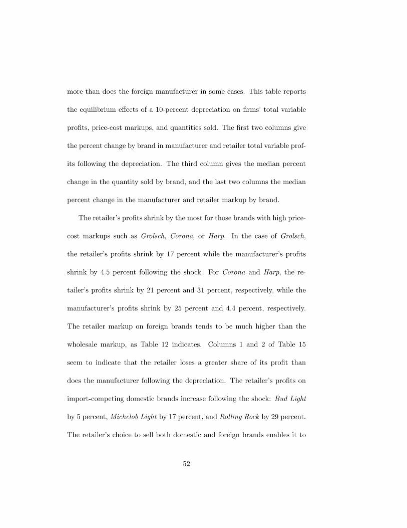
more than does the foreign manufacturer in some cases. This table reports

the equilibrium e¤ects of a 10-percent depreciation on �rms�total variable

pro�ts, price-cost markups, and quantities sold. The �rst two columns give

the percent change by brand in manufacturer and retailer total variable prof-

its following the depreciation. The third column gives the median percent

change in the quantity sold by brand, and the last two columns the median

percent change in the manufacturer and retailer markup by brand.

The retailer�s pro�ts shrink by the most for those brands with high price-

cost markups such as Grolsch, Corona, or Harp. In the case of Grolsch,

the retailer�s pro�ts shrink by 17 percent while the manufacturer�s pro�ts

shrink by 4.5 percent following the shock. For Corona and Harp, the re-

tailer�s pro�ts shrink by 21 percent and 31 percent, respectively, while the

manufacturer�s pro�ts shrink by 25 percent and 4.4 percent, respectively.

The retailer markup on foreign brands tends to be much higher than the

wholesale markup, as Table 12 indicates. Columns 1 and 2 of Table 15

seem to indicate that the retailer loses a greater share of its pro�t than

does the manufacturer following the depreciation. The retailer�s pro�ts on

import-competing domestic brands increase following the shock: Bud Light

by 5 percent, Michelob Light by 17 percent, and Rolling Rock by 29 percent.

The retailer�s choice to sell both domestic and foreign brands enables it to

52

minimize the pro�t loss following the exchange-rate-induced cost shock by

selling more domestic brands.7

6.4 Adjustment in Domestic and Foreign Firms�Pro�ts

Comparing the �rst two columns of Table 15 to the last three columns gives

some indication of the underlying causes of variation in a brand�s total prof-

its: changes in the quantity sold or changes in the markup. The results

indicate that declines in foreign brands�pro�ts result more from declines in

quantities sold than from declines in markups. Those foreign manufactur-

ers who shrink their markups by more than foreign brands�median markup

shrinkage of 8.69 percent lose less total pro�ts than the foreign brands�

median loss of 22.12 percent. By shrinking their markups somewhat ag-

gressively, these foreign manufacturers lose less market share than foreign

brands�median loss of 25.74 percent. The four brands with the smallest

percent declines in manufacturer pro�ts, Sapporo, Molson Light, Grolsch,

and Harp, 1.66 percent, 4.40 percent, 4.44 percent, and 4.44 percent, re-

spectively, are also the brands with the largest percent declines in their

markups: 13.12 percent, 10.09 percent, 16.97 percent, and 13.38 percent,

respectively, and the smallest percent decline in their quantities sold: 21.97

percent, 18.97 percent, 22.90 percent, and 24.20 percent, respectively.

53

6.5 Domestic Versus Foreign Manufacturers

The results suggest some strategic interaction between import-competing

domestic manufacturers and foreign manufacturers following a depreciation:

these domestic manufacturers increase their pro�ts by lowering prices to

take market share from foreign manufacturers. Domestic manufacturers�

pro�ts increase by 1.7 percent following a 10-percent depreciation, mainly

from increases in market share rather than from increases in markups. The

domestic brands with increased pro�ts are the light or superpremium brands

that compete most directly with imported beers.14 As Column 1 of Table

15 shows, only superpremium or light beers�pro�ts rise signi�cantly: Bud

Light by 7.74 percent, Michelob Light by 15.28 percents, Rolling Rock by

27.12 percent, and Special Export by 13.48 percent. Manufacturer pro�ts

increase by more than 1 percent for Bud Light, Coors Light, Michelob Light,

Miller High Life, Miller Lite, Milwaukee�s Best Light, Rolling Rock, and

Special Export. The pro�ts of such sub-premium beers as Busch or Old

Milwaukee change by very little or decline slightly. Those brands in the sub-

premium segment of the market are considered poor substitutes for foreign

brands and so have little to gain from shrinking markups to try to capture

14Table ?? classi�es the domestic brands in the Dominick�s data according to theirmarket segment: subpremium, premium, or superpremium.

54

Post-Depreciation Equilibrium Percent Change

Retailer Pro�t -5.04Domestic Manufacturer Pro�t 1.71Foreign Manufacturer Pro�t -22.12Consumer Surplus -8.18

Total Domestic Welfare -2.85

Table 16: Percent changes in variable pro�ts and consumer surplus followinga 10% depreciation. 4080 observations. Source: My calculations.

market share following a depreciation. These strategic interactions between

domestic and foreign manufacturers provide one possible explanation for

the puzzle of incomplete pass-through. It may not be pro�t maximizing for

foreign manufacturers to fully pass-through a depreciation in a market where

some domestic manufacturers exploit each increase in a foreign brand�s price

to increase their market share.

6.6 Consumer Welfare

Table 16 reports the e¤ect of a 10-percent depreciation on �rms� pro�ts

and on consumer welfare. I �nd that following the depreciation, foreign

manufacturers su¤er the most among the domestic actors, as their total

pro�ts decline by 22.12 percent. Domestic manufacturers bene�t by the most

as their total pro�ts increase by 1.71 percent. Consumer surplus decreases

by 8.18 percent following the depreciation and the retailer�s total pro�ts

55

decline by 5.04 percent.

Table 16 also reports the percent change in total domestic welfare, de-

�ned as the sum of the domestic manufacturers�pro�ts, the domestic re-

tailer�s pro�ts, and the domestic consumer surplus, following each shock.

To compute total domestic welfare, the change in consumer surplus is con-

verted to a dollar �gure by using the compensating variation measure of

Small and Rosen (1981).15 I �nd that total domestic welfare declines by

2.85 percent following a 10 percent depreciation.

7 Conclusion

This paper examines the welfare e¤ects of a change in the nominal exchange

rate using the example of the beer industry. I estimate a structural econo-

metric model that makes it possible to compute manufacturers�and retailers�

pass-through of a nominal exchange-rate change without observing whole-

sale prices or �rms�marginal costs. Using the estimated demand system, I

conduct counterfactual experiments to determine whether domestic manu-

facturers, foreign manufacturers, a domestic retailer, or domestic consumers

bear the cost of a change in the nominal exchange-rate.

The results indicate that foreign manufacturers generally bear more of

15 I describe the details of this compensating variation measure in Appendix B.

56

the cost (or reap more of the bene�t) of a change in the nominal exchange

rate than do domestic consumers, domestic manufacturers, or the domestic

retailer. Following a 10-percent depreciation, foreign manufacturers�pro�ts

decline by 22 percent, while consumer surplus falls by only 8 percent and

the retailer�s pro�ts fall by only 5 percent. The results suggest some strate-

gic interaction between import-competing domestic manufacturers and for-

eign manufacturers following a depreciation. Domestic manufacturers with

brands that are close substitutes for foreign brands increase their pro�ts by

lowering prices to take market share from foreign manufacturers. Domestic

manufacturers�pro�ts increase by 1.7 percent following the depreciation.

In future work, I plan to apply this model to assess the welfare e¤ects

of nominal exchange-rate �uctuations in other industries and economies,

with some emphasis on developing economies. This paper�s approach may

be particularly suited to analyze nominal exchange-rates�welfare e¤ects in

developing countries given their often severe data constraints.16

Finally, analysis of the relationship between market structure and exchange-

rate pass-through may be a promising avenue for future research. Recent

work by Campa and Goldberg (2002) suggests that the variation in pass-

through across countries is more a¤ected by such microeconomic variables as

16As a result, only a handful of published studies estimate exchange-rate pass-throughfor developing economies.

57

the industry composition of each country�s import bundle than by macroeco-

nomic variables. Previous e¤orts to relate industrial organization variables

to exchange-rate pass-through have proven inconclusive. Though several

theoretical papers, most notably Dornbusch (1987), derive theoretical pre-

dictions for the impact of di¤erent market structures on pass-through, no

empirical study has subsequently tested these models�predictions. In fu-

ture work, I plan to extend this paper�s model to examine how di¤erent

vertical contracts between manufacturers and retailers a¤ect exchange-rate

pass-through.

58

References

[1] �Can You Judge a Beer by its Label? Beer Ratings,�Consumer Re-

ports, 10�19 (June 1996).

[2] �The Alcoholic Beverage Market in the United States,�Canadian Trade

Commissioner (June 2000).

[3] Aksoy, Yunus and Yohanes E. Riyanto. �Exchange Rate Pass-Through

in Vertically Related Markets,� Review of International Economics,

8 (2):235�51 (May 2000).

[4] Berry, Steven. �Estimating Discrete-Choice Models of Product Di¤eren-

tiation,�RAND Journal of Economics, 25 (2):242�62 (Summer 1994).

[5] Berry, Steven, et al. �Automobile Prices in Market Equilibrium,�

Econometrica, 63 (4):841�90 (July 1995).

[6] Berry, Steven, et al. �Voluntary Export Restraints on Automobiles:

Evaluating a Trade Policy,� American Economic Review , 89 (3):400�

430 (June 1999).

[7] Blondal, Sveinbjorn and Dirk Pilat. �The Economic Bene�ts of Regu-

latory Reform,�OECD Economic Studies, 28 :7�48 (1997).

59

[8] Bodnar, Gordon M., et al. �Pass-Through and Exposure,�Journal of

Finance, 57 (1):199�231 (February 2002).

[9] Bresnahan, Timothy F. �Departures from Marginal-Cost Pricing in the

American Automobile Industry: Estimates for 1977-1978,� Journal of

Econometrics, 17 (2):201�27 (November 1981).

[10] Bresnahan, Timothy F. �Competition and Collusion in the American

Automobile Industry: The 1955 Price War,�Journal of Industrial Eco-

nomics, 35 (4):457�82 (June 1987).

[11] Bresnahan, Timothy F. �Empirical Studies of Industries with Market

Power.�Handbook of industrial organization VOL 2, edited by Richard

Schmalensee and Robert D. Willig, 1011�57, Amsterdam, Oxford and

Tokyo: North-Holland, 1989.

[12] Bresnahan, Timothy F. and Peter C. Reiss. �Dealer and Manufacturer

Margins,�Rand Journal of Economics, 16 (2):253�68 (Summer 1985).

[13] Calvo, Guillermo A. and Carmen M. Reinhart. �Fear of Floating,�

Quarterly Journal of Economics, 117 (2):379�408 (May 2002).

[14] Campa, Jose Manuel and Linda S. Goldberg. �Investment in Manufac-

turing, Exchange Rates and External Exposure,� Journal of Interna-

60

tional Economics, 38 (3-4):297�320 (May 1995).

[15] Campa, Jose Manuel and Linda S. Goldberg. �The Evolving External

Orientation of Manufacturing: A Pro�le of Four Countries,� Federal

Reserve Bank of New York Economic Policy Review , 3 (2):53�81 (July

1997).

[16] Campa, Jose Manuel and Linda S. Goldberg. �Investment, Pass-

Through, and Exchange Rates: A Cross-Country Comparison,� Inter-

national Economic Review , 40 (2):287�314 (May 1999).

[17] Campa, Jose Manuel and Linda S. Goldberg. �Exchange-Rate Pass-

Through into Import Prices: A Macro or Micro Phenomenon?,�NBER

Working Paper , 8934 (May 2002).

[18] Chevalier, Judith A., et al. �Why Don�t Prices Rise during Periods

of Peak Demand? Evidence from Scanner Data,�American Economic

Review , 93 (1):15�37 (March 2003).

[19] Citrin, Daniel. �The Recent Behavior of US Trade Prices,� Interna-

tional Monetary Fund Working Paper , 89/29 (April 1989).

[20] Corsetti, Giancarlo et al. �Competitive Devaluations: Toward

a Welfare-Based Approach,� Journal of International Economics,

61

51 (1):217�41 (June 2000).

[21] Desiraju, Ramarao and Milind Shrikhande. �Exchange Rate Pass-

Through and the Role of International Distribution Channels,� Inter-

national Journal of Business, 2 (2):1�28 (1997).

[22] Devereux, Michael B., et al. �Exchange Rate Pass-Through and

the Welfare E¤ects of the Euro,� International Economic Review ,

44 (1):223�42 (February 2003).

[23] Devereux, Michael B. and Phillip R. Lane. �Understanding Bilat-

eral Exchange-Rate Volatility,� Journal of International Economics,

60 (1):109�32 (2003).

[24] Dornbusch, Rudiger. �Exchange Rates and Prices,� American Eco-

nomic Review , 77 (1):93�106 (March 1987).

[25] Dunn, Robert M. Jr. �Flexible Exchange Rates and Oligopoly Pric-

ing: A Study of Canadian Markets,� Journal of Political Economy ,

78 (1):140�51 (January-February 1970).

[26] Engel, Charles. �Local-Currency Pricing and the Choice of Exchange-

Rate Regime,� European Economic Review , 44 (8):1449�72 (August

2000).

62

[27] Engel, Charles and John H. Rogers. �How Wide Is the Border?,�Amer-

ican Economic Review , 86 (5):1112�25 (December 1996).

[28] Engel, Charles and John H. Rogers. �Relative Price Volatility: What

Role Does the Border Play?.�Intranational macroeconomics edited by

Gregory D. Hess and Eric van Wincoop, 92�111, Cambridge, New York

and Melbourne: Cambridge University Press, 2000.

[29] Engel, Charles and John H. Rogers. �Deviations from Purchasing

Power Parity: Causes and Welfare Costs,� Journal of International

Economics, 55 (1):29�57 (October 2001).

[30] Feenstra, Robert C. �Symmetric Pass-Through of Tari¤s and Exchange

Rates Under Imperfect Competition: An Empirical Test,� Journal of

International Economics, 27 :25�45 (1989).

[31] Feenstra, Robert C., et al. �Market Share and Exchange Rate Pass-

Through in World Automobile Trade,� Journal of International Eco-

nomics, 40 (1-2):187�207 (February 1996).

[32] Feinberg, Robert M. �The Interaction of Foreign Exchange and Mar-

ket Power E¤ects on German Domestic Prices,� Journal of Industrial

Economics, 35 (1):61�70 (September 1986).

63

[33] Feinberg, Robert M. �The E¤ects of Foreign Exchange Movements on

US Domestic Prices,�Review of Economics and Statistics, 71 (3):505�

11 (August 1989).

[34] Feinberg, Robert M. �The Role of International Discipline in Three

Developing Economies: Exchange Rate E¤ects on Domestic Prices in

Colombia, Korea, and Morocco,�Review of International Economics,

8 (1):126�33 (February 2000).

[35] Fisher, Eric. �A Model of Exchange Rate Pass-Through,� Journal of

International Economics, 26 (1-2):119�37 (February 1989).

[36] Froot, Kenneth A. and Paul D. Klemperer. �Exchange Rate Pass-

Through When Market Share Matters,�American Economic Review ,

79 (4):637�54 (September 1989).

[37] Gagnon, Joseph E. and Michael M. Knetter. �Markup Adjustment and

Exchange Rate Fluctuations: Evidence from Panel Data on Automobile

Exports,�Journal of International Money and Finance, 14 (2):289�310

(April 1995).

[38] Gasmi, F., et al. �Econometric Analysis of Collusive Behavior in a

Soft-Drink Market,�Journal of Economics and Management Strategy ,

1 (2):277�311 (Summer 1992).

64

[39] Goldberg, Pinelopi Koujianou. �Product Di¤erentiation and Oligopoly

in International Markets: The Case of the US Automobile Industry,�

Econometrica, 63 (4):891�951 (July 1995).

[40] Goldberg, Pinelopi Koujianou and Michael M. Knetter. �Goods Prices

and Exchange Rates: What Have We Learned?,�Journal of Economic

Literature, 35 (3):1243�72 (September 1997).

[41] Goldberg, Pinelopi Koujianou and Michael M. Knetter. �Measuring the

Intensity of Competition in Export Markets,�Journal of International

Economics, 47 (1):27�60 (February 1999).

[42] Gron, Anne and Deborah L. Swenson. �Incomplete Exchange-Rate

Pass-Through and Imperfect Competition: The E¤ect of Local Pro-

duction,�American Economic Review , 86 (2):71�76 (May 1996).

[43] Gron, Anne and Deborah L. Swenson. �Cost Pass-Through in the US

Automobile Market,�Review of Economics and Statistics, 82 (2):316�

24 (May 2000).

[44] Hausman, Jerry, et al. �Competitive Analysis with Di¤erenciated Prod-

ucts,� Annales d�Economie et de Statistique, 34 :159�80 (April-June

1994).

65

[45] Hooper, Peter and Catherine L. Mann. �Exchange Rate Pass-Through

in the 1980s: The Case of US Imports of Manufacturers,� Brookings

Papers on Economic Activity , 297�329 (1989).

[46] Hummels, David, et al. �The Nature and Growth of Vertical Specializa-

tion in World Trade,�Journal of International Economics, 54 (1):75�96

(June 2001).

[47] Hummels, David, et al. �Vertical Specialization and the Changing Na-

ture of World Trade,� Federal Reserve Bank of New York Economic

Policy Review , 4 (2):79�99 (June 1998).

[48] Kadiyali, Vrinda. �Exchange Rate Pass-through for Strategic Pricing

and Advertising: An Empirical Analysis of the US Photographic Film

Industry,� Journal of International Economics, 43 (3-4):437�61 (No-

vember 1997).

[49] Kadiyali, Vrinda, et al. �Manufacturer-Retailer Channel Interactions

and Implications for Channel Power: An Empirical Investigation of

Pricing in a Local Market,�Marketing Science, 19 (2):127�48 (Spring

2000).

[50] Katz, Michael L. �Vertical Contractual Relations.�Handbook of indus-

trial organization VOL 1, edited by Richard Schmalensee and Robert D.

66

Willig, 655�721, Amsterdam, Oxford and Tokyo: North-Holland, 1989.

[51] Knetter, Michael M. �Price Discrimination by US and German Ex-

porters,�American Economic Review , 79 (1):198�210 (March 1989).

[52] Knetter, Michael M. �International Comparisons of Price-to-Market

Behavior,�American Economic Review , 83 (3):473�86 (June 1993).

[53] Kose, M. Ayhan and Kei Mu Yi. �International Trade and Business Cy-

cles: Is Vertical Specialization the Missing Link?,�American Economic

Review , 91 (2):371�75 (May 2001).

[54] Krugman, Paul R. �Pricing to Market When the Exchange Rate

Changes.� Real-�nancial linkages among open economies edited by

Sven W. Arndt and J. David Richardson, 49�70, Cambridge, MA and

London: MIT Press, 1987.

[55] Lee, Eunkyu and Richard Staelin. �Vertical Strategic Interac-

tion: Implications for Channel Pricing Strategy,�Marketing Science,

16 (3):185�207 (1997).

[56] Mann, Catherine L. �Prices, Pro�t Margins, and Exchange Rates,�

Federal Reserve Bulletin, 72 (6):366�79 (June 1986).

67

[57] McCarthy, Jonathan. �Pass-Through of Exchange Rates and Import

Prices to Domestic In�ation in Some Industrialized Economies,�Federal

Reserve Bank of New York Sta¤ Reports, 111 (2000).

[58] McFadden, Daniel. �Conditional Logit Analysis of Qualitative Choice

Behavior.�Frontiers of econometrics edited by Paul Zarembka, 105�42,

New York: Academic Press, 1973.

[59] McFadden, Daniel. �Econometric Models of Probabilistic Choice.�

Structural analysis of discrete data edited by Charles F. Manski and

Daniel McFadden, 169�73, Cambridge: MIT Press, 1981.

[60] McFadden, Daniel and Kenneth Train. �Mixed MNL Models for

Discrete Response,� Journal of Applied Econometrics, 15 (5):447�70

(September-October 2000).

[61] Menon, Jayant. �Exchange Rate Pass-Through,�Journal of Economic

Surveys, 9 (2):197�231 (June 1995).

[62] Nevo, Aviv. �Mergers with Di¤erentiated Products: The Case of

the Ready-to-Eat Cereal Industry,� RAND Journal of Economics,

31 (3):395�421 (Autumn 2000).

68

[63] Nevo, Aviv. �A Practitioner�s Guide to Estimation of Random-

Coe¢ cients Logit Models of Demand,�Journal of Economics and Man-

agement Strategy , 9 (4):513�48 (Winter 2000).

[64] Nevo, Aviv. �Measuring Market Power in the Ready-to-Eat Cereal

Industry,�Econometrica, 69 (2):307�42 (March 2001).

[65] Rangan, Subramanian and Robert Z. Lawrence. �The Responses of US

Firms to Exchange Rate Fluctuations: Piercing the Corporate Veil,�

Brookings Papers on Economic Activity , 341�69 (1993).

[66] Rogo¤, Kenneth. �The Purchasing Power Parity Puzzle,� Journal of

Economic Literature, 34 (2):647�68 (June 1996).

[67] Rogo¤, Kenneth. �Perspectives on Exchange Rate Volatility.�NBER

Conference Report series International capital �ows, edited by Martin

Feldstein, 441�53, Chicago and London: University of Chicago Press,

1999.

[68] Scherer, Frederic M. �Retail Distribution Channel Barriers to Interna-

tional Trade.�Competition policy, domestic and international. Econo-

mists of the Twentieth Century series, edited by Frederic M. Scherer,

406�41, Cheltenham, UK and Northampton, MA: Elgar, 2000.

69

[69] Sibert, Anne. �Exchange Rates, Market Structure, Prices and Imports,�

Economic Record , 68 (202):233�39 (September 1992).

[70] Small, Kenneth A. and Harvey S. Rosen. �Applied Welfare Economics

with Discrete Choice Models,� Econometrica, 49 (1):105�30 (January

1981).

[71] Staiger, Douglas and James H. Stock. �Instrumental Variables Regres-

sion with Weak Instruments,�Econometrica, 65 (3):557�86 (May 1997).

[72] Sudhir, K. �Structural Analysis of Manufacturer Pricing in the Pres-

ence of a Strategic Retailer,�Marketing Science, 20 (3):244�64 (Sum-

mer 2001).

[73] Tille, Cedric. �The Role of Consumption Substitutability in the Inter-

national Transmission of Monetary Shocks,� Journal of International

Economics, 53 (2):421�44 (April 2001).

[74] Tirole, Jean. The theory of industrial organization. Cambridge, MA

and London: MIT Press, 1988.

[75] Train, Kenneth. Discrete choice with simulation. Cambridge: Cam-

bridge University Press, 2003.

70

[76] Villas-Boas, So�a Berto. Vertical Relationships between Manufacturers

and Retailers. PhD dissertation, U.C. Berkeley, May 2002.

[77] Yi, Kei Mu. �Can Vertical Specialization Explain the Growth of World

Trade?,�Journal of Political Economy , 111 (1):52�102 (February 2003).

71

A Welfare Calculations

The structural model I use enables me to calculate the change in consumer

welfare following an exchange-rate shock. This change can be given a dollar

�gure by using the compensating variation measure of Small and Rosen

(1981) which for individual i is de�ned as:

CVi = �lnhPJ

j=0 eV postij

i� ln

hPJj=0 e

V preij

i�i

(23)

where V preij is consumer i�s indirect utility from consuming product j

given its price before the exchange-rate shock, V postij is her indirect utility

from consuming the same product given its price after the exchange-rate

shock, and �i is her marginal utility of income which one must assume does

not vary following the price change. V postij and V pre

ij are de�ned in equation

(8 ) . This calculation assumes that the perceived characteristics of all the

products, including the outside good, do not change over the period of the

exchange-rate shock. I calculate the compensating variation for each of

the 40 individuals I sample for each price zone. As the income e¤ects for

purchases of beer are minimal, this compensating variation measure equals

the equivalent variation for each of the 40 individuals sampled in each price

zone. The dollar value of the change in consumer surplus is given by the

72

average compensating variation across these individuals multiplied by the

population of the relevant market.

I calculate the change in total domestic welfare as the sum of this com-

pensating variation measure, the change in domestic manufacturers�pro�ts,

and the change in the domestic retailer�s pro�ts following the exchange-rate

shock.

73

B Supplementary Tables

HO ModelDouble DoubleMarginalization Marginalization

HA Model with Foreign Collusion

1. Double Marginalization (DM) 10.252. DM with Foreign Collusion .89

Table 17: Results from non-nested tests to determine which vertical contractmodel best explains the data. Each column has the null model being testedand each row the alternative model against which it is being tested. Non-nestedCox-type tests can be discriminated using a Vuong (1989) and Villas-Boas (2002)two-step procedure and are distributed standard normal. One-sided test statisticat 5 percent signi�cance levels is 1.65.

74

Product Wholesale Con�dence Manufacturer Con�dencePrice Interval Marginal Cost Interval

Domestic BrandsBudweiser 37.48 36.92-38.18 28.75 27.67-29.64Bud Light 37.49 36.80-38.34 27.73 26.71-28.39Busch 35.70 34.63-36.19 26.48 25.97-27.49Busch Light 31.53 31.03-32.44 23.38 22.83-23.98Coors 35.48 34.79-36.21 26.98 26.41-28.02Coors Light 36.27 35.68-36.97 27.23 26.24-28.05Keystone 25.86 25.40-26.31 19.04 18.60-19.69Michelob Light 41.98 41.12-43.39 30.81 30.18-32.37Miller Genuine Draft 37.46 36.90-38.26 28.91 27.97-29.81Miller High Life 37.59 36.68-38.44 28.18 26.96-28.56Miller Lite 36.60 36.06-37.61 27.54 26.71-28.52Milwaukee�s Best 28.26 27.25-28.96 19.42 19.06-20.66Milwaukee�s Best Lite 35.13 34.63-35.50 24.84 24.34-25.72Old Milwaukee 21.54 20.97-22.38 13.89 13.38-15.37Old Style 42.72 41.76-44.05 31.63 30.91-32.55Old Style Classic 34.23 33.15-35.23 25.88 25.54-26.73Rolling Rock 47.31 45.70-48.58 33.69 32.37-35.81Special Export 44.25 43.22-45.58 32.90 31.82-34.44Stroh�s 30.02 29.51-30.45 22.64 22.06-23.22All Domestic Brands 36.02 35.79-36.24 26.77 26.50-27.05European BrandsBeck�s 62.70 60.49-65.55 41.94 39.06-44.62St. Pauli 73.41 71.01-75.62 50.47 47.07-55.81Amstel 70.26 66.65-72.68 45.86 42.67-52.07Grolsch 82.58 80.93-86.19 58.74 56.29-62.01Heineken 70.70 67.72-72.40 47.10 45.05-53.25Harp 82.95 78.59-85.27 59.43 52.46-62.11Peroni 67.08 63.89-70.31 45.52 42.71-49.61Bass 83.83 81.73-87.86 60.55 57.06-64.50North American BrandsFoster�s 76.45 73.64-79.73 53.23 49.11-58.01Guinness 85.49 83.20-89.54 61.32 56.36-65.33Molson Golden 55.19 54.08-59.09 42.10 40.37-44.80Molson Light 51.55 48.81-56.75 32.50 28.60-38.48Corona 67.14 64.11-70.26 45.40 42.49-49.61Tecate 64.02 61.32-65.77 41.83 39.51-45.44Japanese BrandsSapporo 76.31 74.54-79.75 53.48 47.84-55.69All Foreign Brands 71.30 70.35-72.34 48.69 47.68-49.88All Brands 43.58 42.81-44.54 32.22 31.80-32.65

Table 18: 95-percent con�dence intervals for the median of the derived mar-ginal costs for the 34 products in the sample. Median in cents per 12-ounceserving across 120 markets. Con�dence intervals calculated using 10,000 bootstrapsamples (with replacement). 4080 observations. Source: My calculations.

75

Product MarginMan. Ret. Vert.% % %

Domestic BrandsBudweiser 22.51 26.70 43.44Bud Light 24.20 29.64 47.54Busch 22.66 25.68 42.83Busch Light 25.20 27.65 46.10Coors 22.93 27.69 44.16Coors Light 24.12 29.21 45.52Keystone 24.72 26.83 45.12Michelob Light 24.76 29.77 48.28Miller Genuine Draft 23.01 26.58 43.28Miller High Life 25.09 26.58 44.26Miller Lite 24.49 28.26 45.77Milwaukee�s Best 27.23 25.66 45.24Milwaukee�s Best Lite 26.77 27.52 46.93Old Milwaukee 33.46 34.71 56.80Old Style 23.53 28.35 46.44Old Style Classic 22.02 25.87 42.17Rolling Rock 26.87 30.99 49.90Special Export 23.71 28.59 46.03Stroh�s 23.57 26.98 43.94All Domestic Brands 24.42 27.39 45.50European BrandsBeck�s 33.15 31.91 55.46St. Pauli 31.14 29.16 51.70Amstel 33.89 30.88 55.08Grolsch 30.34 27.38 49.74Heineken 31.86 30.04 53.40Harp 30.64 27.32 50.10Peroni 32.93 30.43 54.00Bass 29.47 26.90 48.81Other Foreign BrandsFoster�s 31.78 28.81 51.68Guinness 30.59 27.47 50.24Molson Golden 23.78 28.69 45.95Molson Light 38.40 35.62 61.71Corona 33.20 30.54 54.21Tecate 33.65 31.72 54.95Sapporo 32.66 29.60 53.33All Foreign Brands 30.72 29.70 51.72

Table 19: Median derived price-cost margins by product. Median across 120markets. The margin is markup divided by price with units in percentages. Source:My calculations.

76

Country Mean Median Std Minimum MaximumCanada 19.33 19.21 .74 17.79 19.33Germany 35.09 35.16 2.65 31.65 38.32Holland 38.31 38.84 2.00 35.58 40.57Ireland 8.21 8.27 .45 7.63 8.78Italy 25397.40 25678 1621.49 23161 26853Japan 1615 1619 63.68 1533 1688Mexico 2111.48 8.59 2895.06 6.35 5670United Kingdom 7.84 7.86 .24 7.48 8.14United States 15.01 15.12 .58 14.14 15.63

Table 20: Instruments: Hourly wages in local-currency terms. Annual data.Hourly compensation for production workers in food, beverage, and tobaccomanufacturing industries, SIC 20 and 21. Source: Foreign Labor Statistics,Bureau of Labor Statistics, U.S. Department of Labor.

77

Product Elasticities Con�denceIntervals

Domestic BrandsBudweiser -6.37 -6.57 to -6.11Bud Light -5.88 -6.19 to -5.70Busch -6.49 -6.70 to -6.24Busch Light -6.02 -6.26 to -5.83Coors -6.34 -6.53 to -6.11Coors Light -5.99 -6.23 to -5.73Keystone -5.85 -5.98 to -5.63Michelob Light -6.05 -6.35 to -5.81Miller Genuine Draft -5.91 -6.05 to -5.71Miller High Life -6.49 -6.69 to -6.27Miller Lite -5.61 -5.85 to -5.50Milwaukee�s Best -6.09 -6.28 to -5.88Milwaukee�s Best Light -6.27 -6.49 to -6.05Old Milwaukee -4.75 -4.94 to -4.59Old Style -6.25 -6.64 to -6.08Old Style Classic -6.21 -6.35 to -6.01Rolling Rock -5.95 -6.36 to -5.72Special Export -6.25 -6.77 to -6.15Stroh�s -6.11 -6.32 to -5.86European BrandsBeck�s -5.71 -6.39 to -5.46St. Pauli -6.31 -7.11 to -5.88Amstel -6.06 -6.86 to -5.76Grolsch -6.70 -7.78 to -6.29Heineken -6.12 -6.96 to -5.73Harp -6.70 -7.56 to -6.10Peroni -6.06 -6.82 to -5.59Bass -6.85 -7.59 to -6.34North American BrandsFoster�s -6.39 -7.34 to -6.04Guinness -6.67 -7.36 to -6.18Molson Golden -6.73 -7.19 to -6.36Molson Light -5.21 -5.76 to -4.83Corona -6.04 -6.77 to -5.55Tecate -5.97 -6.63 to -5.57Japanese BrandsSapporo -6.22 -7.08 to -5.91

Table 21: Median own-price demand elasticities. Median across all 120 mar-kets. 95 percent con�dence intervals generated with bootstrap simulations.4080 observations. Source: My calculations.

78