What to do when K-means clustering fails - Max Little

What to do when K-means clustering fails: a simple yetprincipled alternative algorithmYordan P. Raykov1,†,*, Alexis Boukouvalas2,†, Fahd Baig3, Max A. Little1,4

1 School of Mathematics, Aston University, Birmingham, United Kingdom2 Molecular Sciences, University of Manchester, Manchester, UnitedKingdom3 Nuffield Department of Clinical Neurosciences, Oxford University,Oxford, United Kingdom4 Media Lab, Massachusetts Institute of Technology, Cambridge,Massachusetts, United States

†These authors contributed equally to this work.* [email protected]

AbstractThe K-means algorithm is one of the most popular clustering algorithms in

current use as it is relatively fast yet simple to understand and deploy in practice.Nevertheless, its use entails certain restrictive assumptions about the data, thenegative consequences of which are not always immediately apparent, as wedemonstrate. While more flexible algorithms have been developed, theirwidespread use has been hindered by their computational and technical complexity.Motivated by these considerations, we present a flexible alternative to K-meansthat relaxes most of the assumptions, whilst remaining almost as fast and simple.This novel algorithm which we call MAP-DP (maximum a-posteriori Dirichletprocess mixtures), is statistically rigorous as it is based on nonparametric BayesianDirichlet process mixture modeling. This approach allows us to overcome most ofthe limitations imposed by K-means. The number of clusters K is estimated fromthe data instead of being fixed a-priori as in K-means. In addition, whileK-means is restricted to continuous data, the MAP-DP framework can be appliedto many kinds of data, for example, binary, count or ordinal data. Also, it canefficiently separate outliers from the data. This additional flexibility does notincur a significant computational overhead compared to K-means with MAP-DPconvergence typically achieved in the order of seconds for many practical problems.Finally, in contrast to K-means, since the algorithm is based on an underlyingstatistical model, the MAP-DP framework can deal with missing data and enablesmodel testing such as cross validation in a principled way. We demonstrate thesimplicity and effectiveness of this algorithm on the health informatics problem ofclinical sub-typing in a cluster of diseases known as parkinsonism.

1 IntroductionThe rapid increase in the capability of automatic data acquisition and storage isproviding a striking potential for innovation in science and technology. However,extracting meaningful information from complex, ever-growing data sources poses newchallenges. This motivates the development of automated ways to discover underlyingstructure in data. The key information of interest is often obscured behind redundancyand noise, and grouping the data into clusters with similar features is one way of

1/35

efficiently summarizing the data for further analysis [1]. Cluster analysis has been usedin many fields [1, 2], such as information retrieval [3], social media analysis [4],neuroscience [5], image processing [6], text analysis [7] and bioinformatics [8].

Despite the large variety of flexible models and algorithms for clustering available,K-means remains the preferred tool for most real world applications [9]. K-means wasfirst introduced as a method for vector quantization in communication technologyapplications [10], yet it is still one of the most widely-used clustering algorithms. Forexample, in discovering sub-types of parkinsonism, we observe that most studies haveused K-means algorithm to find sub-types in patient data [11]. It is also the preferredchoice in the visual bag of words models in automated image understanding [12].Perhaps the major reasons for the popularity of K-means are conceptual simplicity andcomputational scalability, in contrast to more flexible clustering methods. Bayesianprobabilistic models, for instance, require complex sampling schedules or variationalinference algorithms that can be difficult to implement and understand, and are oftennot computationally tractable for large data sets.

For the ensuing discussion, we will use the following mathematical notation todescribe K-means clustering, and then also to introduce our novel clustering algorithm.Let us denote the data as X = (x1, . . . , xN ) where each of the N data points xi is aD-dimensional vector. We will denote the cluster assignment associated to each datapoint by z1, . . . , zN , where if data point xi belongs to cluster k we write zi = k. Thenumber of observations assigned to cluster k, for k ∈ 1, . . . ,K, is Nk and N−ik is thenumber of points assigned to cluster k excluding point i. The parameter ε > 0 is a smallthreshold value to assess when the algorithm has converged on a good solution andshould be stopped (typically ε = 10−6). Using this notation, K-means can be written asin Algorithm 1.

To paraphrase this algorithm: it alternates between updating the assignments ofdata points to clusters while holding the estimated cluster centroids, µk, fixed (lines5-11), and updating the cluster centroids while holding the assignments fixed (lines14-15). It can be shown to find some minimum (not necessarily the global, i.e. smallestof all possible minima) of the following objective function:

E = 12

K∑k=1

∑i:zi=k

‖xi − µk‖22 (1)

with respect to the set of all cluster assignments z and cluster centroids µ, where 12 ‖.‖

22

denotes the Euclidean distance (distance measured as the sum of the square ofdifferences of coordinates in each direction). In fact, the value of E cannot increase oneach iteration, so, eventually E will stop changing (tested on line 17).

Perhaps unsurprisingly, the simplicity and computational scalability of K-meanscomes at a high cost. In particular, the algorithm is based on quite restrictiveassumptions about the data, often leading to severe limitations in accuracy andinterpretability:

1. By use of the Euclidean distance (algorithm line 9) K-means treats the data spaceas isotropic (distances unchanged by translations and rotations). This means thatdata points in each cluster are modeled as lying within a sphere around the clustercentroid. A sphere has the same radius in each dimension. Furthermore, asclusters are modeled only by the position of their centroids, K-means implicitlyassumes all clusters have the same radius. When this implicit equal-radius,spherical assumption is violated, K-means can behave in a non-intuitive way, evenwhen clusters are very clearly identifiable by eye (see Figs 1, 2 and discussion inSections 5.1, 5.4).

2/35

Algorithm 1: K-means Algorithm 2: MAP-DP(spherical Gaussian)

Input x1, . . . , xN : D-dimensionaldataε > 0: convergence thresholdK: number of clusters

x1, . . . , xN : D-dimensional dataε > 0: convergence thresholdN0: prior countσ̂2: spherical cluster varianceσ2

0 : prior centroid varianceµ0: prior centroid location

Output z1, . . . , zN : clusterassignmentsµ1, . . . , µK : cluster centroids

z1, . . . , zN : cluster assignmentsK: number of clusters

1 Set µk for all k ∈ 1, . . . ,K 1 K = 1, zi = 1 for all i ∈ 1, . . . , N2 Enew =∞ 2 Enew =∞3 repeat 3 repeat4 Eold = Enew 4 Eold = Enew5 for i ∈ 1, . . . , N 5 for i ∈ 1, . . . , N6 for k ∈ 1, . . . ,K 6 for k ∈ 1, . . . ,K7 7 σ−ik =

(1σ2

0+ 1

σ̂2N−ik

)−1

8 8 µ−ik = σ−ik

(µ0σ2

0+ 1

σ̂2

∑j:zj=k,j 6=i xj

)9 di,k = 1

2 ‖xi − µk‖22 9 di,k = 1

2(σ−ik

+σ̂2)∥∥xi − µ−ik ∥∥2

2

+D2 ln

(σ−ik + σ̂2)

10 10 di,K+1 = 12(σ2

0+σ̂2) ‖xi − µ0‖22+D

2 ln(σ2

0 + σ̂2)11 zi = arg mink∈1,...,K di,k 11 zi = arg mink∈1,...,K+1

[di,k − lnN−ik

]12 12 if zi = K + 113 13 K = K + 114 for k ∈ 1, . . . ,K 1415 µk = 1

Nk

∑j:zj=k xj 15

16 Enew =∑Kk=1

∑i:zi=k di,k 16 Enew =

∑Kk=1

∑i:zi=k di,k

−K lnN0 −∑Kk=1 log Γ (Nk)

17 until Eold − Enew < ε 17until Eold − Enew < ε

3/35

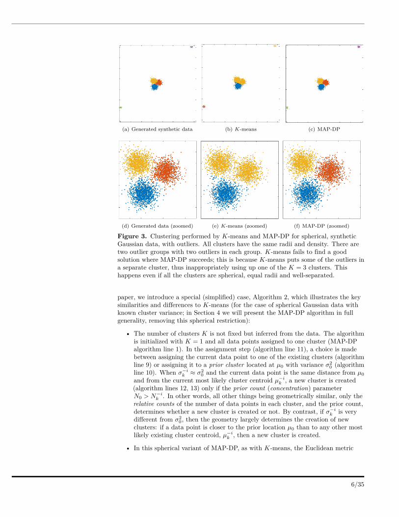
(a) Generated synthetic data (b) K-means (c) MAP-DP

Figure 1. Clustering performed by K-means and MAP-DP for spherical, syntheticGaussian data, with unequal cluster radii and density. The clusters are well-separated.Data is equally distributed across clusters. Here, unlike MAP-DP, K-means fails to findthe correct clustering. Instead, it splits the data into three equal-volume regionsbecause it is insensitive to the differing cluster density. Different colours indicate thedifferent clusters.

2. The Euclidean distance entails that the average of the coordinates of data pointsin a cluster is the centroid of that cluster (algorithm line 15). Euclidean space islinear which implies that small changes in the data result in proportionately smallchanges to the position of the cluster centroid. This is problematic when there areoutliers, that is, points which are unusually far away from the cluster centroid bycomparison to the rest of the points in that cluster. Such outliers can dramaticallyimpair the results of K-means (see Fig 3 and discussion in Section 5.3).

3. K-means clusters data points purely on their (Euclidean) geometric closeness tothe cluster centroid (algorithm line 9). Therefore, it does not take into accountthe different densities of each cluster. So, because K-means implicitly assumeseach cluster occupies the same volume in data space, each cluster must containthe same number of data points. We will show later that even when all otherimplicit geometric assumptions of K-means are satisfied, it will fail to learn acorrect, or even meaningful, clustering when there are significant differences incluster density (see Fig 4 and Section 5.2).

4. The number K of groupings in the data is fixed and assumed known; this is rarelythe case in practice. Thus, K-means is quite inflexible and degrades badly whenthe assumptions upon which it is based are even mildly violated by e.g. a tinynumber of outliers (see Fig 3 and discussion in Section 5.3).

Some of the above limitations of K-means have been addressed in the literature.Regarding outliers, variations of K-means have been proposed that use more “robust”estimates for the cluster centroids. For example, the K-medoids algorithm uses the pointin each cluster which is most centrally located. By contrast, in K-medians the medianof coordinates of all data points in a cluster is the centroid. However, both approachesare far more computationally costly than K-means. K-medoids, requires computationof a pairwise similarity matrix between data points which can be prohibitively expensivefor large data sets. In K-medians, the coordinates of cluster data points in eachdimension need to be sorted, which takes much more effort than computing the mean.

Provided that a transformation of the entire data space can be found which“spherizes” each cluster, then the spherical limitation of K-means can be mitigated.However, for most situations, finding such a transformation will not be trivial and is

4/35


Figure 2. Clustering solution obtained by K-means and MAP-DP for syntheticelliptical Gaussian data. All clusters share exactly the same volume and density, butone is rotated relative to the others. There is no appreciable overlap. K-means failsbecause the objective function which it attempts to minimize measures the trueclustering solution as worse than the manifestly poor solution shown here.

usually as difficult as finding the clustering solution itself. Alternatively, by using theMahalanobis distance, K-means can be adapted to non-spherical clusters [13], but thisapproach will encounter problematic computational singularities when a cluster has onlyone data point assigned.

Addressing the problem of the fixed number of clusters K, note that it is notpossible to choose K simply by clustering with a range of values of K and choosing theone which minimizes E. This is because K-means is nested: we can always decrease Eby increasing K, even when the true number of clusters is much smaller than K, since,all other things being equal, K-means tries to create an equal-volume partition of thedata space. Therefore, data points find themselves ever closer to a cluster centroid as Kincreases. In the extreme case for K = N (the number of data points), then K-meanswill assign each data point to its own separate cluster and E = 0, which has no meaningas a “clustering” of the data. Various extensions to K-means have been proposed whichcircumvent this problem by regularization over K, e.g. Akaike (AIC) or Bayesianinformation criteria (BIC), and we discuss this in more depth in Section 3).

So far, we have presented K-means from a geometric viewpoint. However, it can alsobe profitably understood from a probabilistic viewpoint, as a restricted case of the(finite) Gaussian mixture model (GMM). This is the starting point for us to introduce anew algorithm which overcomes most of the limitations of K-means described above.

This new algorithm, which we call maximum a-posteriori Dirichlet process mixtures(MAP-DP), is a more flexible alternative to K-means which can quickly provideinterpretable clustering solutions for a wide array of applications.

By contrast to K-means, MAP-DP can perform cluster analysis without specifyingthe number of clusters. In order to model K we turn to a probabilistic framework whereK grows with the data size, also known as Bayesian non-parametric (BNP) models [14].In particular, we use Dirichlet process mixture models (DP mixtures) where the numberof clusters can be estimated from data. To date, despite their considerable power,applications of DP mixtures are somewhat limited due to the computationally expensiveand technically challenging inference involved [15, 16, 17]. Our new MAP-DP algorithmis a computationally scalable and simple way of performing inference in DP mixtures.Additionally, MAP-DP is model-based and so provides a consistent way of inferringmissing values from the data and making predictions for unknown data.

As a prelude to a description of the MAP-DP algorithm in full generality later in the

5/35


(d) Generated data (zoomed) (e) K-means (zoomed) (f) MAP-DP (zoomed)

Figure 3. Clustering performed by K-means and MAP-DP for spherical, syntheticGaussian data, with outliers. All clusters have the same radii and density. There aretwo outlier groups with two outliers in each group. K-means fails to find a goodsolution where MAP-DP succeeds; this is because K-means puts some of the outliers ina separate cluster, thus inappropriately using up one of the K = 3 clusters. Thishappens even if all the clusters are spherical, equal radii and well-separated.

paper, we introduce a special (simplified) case, Algorithm 2, which illustrates the keysimilarities and differences to K-means (for the case of spherical Gaussian data withknown cluster variance; in Section 4 we will present the MAP-DP algorithm in fullgenerality, removing this spherical restriction):

• The number of clusters K is not fixed but inferred from the data. The algorithmis initialized with K = 1 and all data points assigned to one cluster (MAP-DPalgorithm line 1). In the assignment step (algorithm line 11), a choice is madebetween assigning the current data point to one of the existing clusters (algorithmline 9) or assigning it to a prior cluster located at µ0 with variance σ2

0 (algorithmline 10). When σ−ik ≈ σ2

0 and the current data point is the same distance from µ0and from the current most likely cluster centroid µ−ik , a new cluster is created(algorithm lines 12, 13) only if the prior count (concentration) parameterN0 > N−ik . In other words, all other things being geometrically similar, only therelative counts of the number of data points in each cluster, and the prior count,determines whether a new cluster is created or not. By contrast, if σ−ik is verydifferent from σ2

0 , then the geometry largely determines the creation of newclusters: if a data point is closer to the prior location µ0 than to any other mostlikely existing cluster centroid, µ−ik , then a new cluster is created.

• In this spherical variant of MAP-DP, as with K-means, the Euclidean metric

6/35

12 ‖.‖

22 is used to compute distances to cluster centroids (algorithm lines 9, 10).

However, in MAP-DP, the log of N−ik is subtracted from this distance whenupdating assignments (algorithm line 11). Also, the composite variance σ−ik + σ̂2

features in the distance calculations such that the smaller σ−ik + σ̂2 becomes, theless important the number of data points in the cluster N−ik becomes to theassignment. In that case, the algorithm behaves much like K-means. But, ifσ−ik + σ̂2 becomes large, then, if a cluster already has many data points assignedto it, it is more likely that the current data point is assigned to that cluster (inother words, clusters exhibit a “rich-get-richer” effect). MAP-DP thereby takesinto account the density of clusters, unlike K-means. We can see σ−ik + σ̂2 ascontrolling the “balance” between geometry and density.

• MAP-DP directly estimates only cluster assignments, while K-means also findsthe most likely cluster centroids given the current cluster assignments. But, sincethe cluster assignment estimates may be significantly in error, this error willpropagate to the most likely cluster centroid locations. By contrast, MAP-DPnever explicitly estimates cluster centroids, they are treated as appropriatelyuncertain quantities described by a most likely cluster location µ−ik and varianceσ−ik (the centroid hyper parameters). This means that MAP-DP does not needexplicit values of the cluster centroids on initialization (K-means algorithm line 1).Indeed, with K-means, poor choices of these initial cluster centroids can cause thealgorithm to fall into sub-optimal configurations from which it cannot recover,and there is, generally, no known universal way to pick “good” initial centroids.At the same time, during iterations of the algorithm, MAP-DP can bypasssub-optimal, erroneous configurations that K-means cannot avoid. This alsomeans that MAP-DP often converges in many fewer iterations than K-means. Aswe discuss in Appendix D cluster centroids and variances can be obtained inMAP-DP if needed after the algorithm has converged.

• The cluster hyper parameters are updated explicitly for each data point in turn(algorithm lines 7, 8). This updating is a weighted sum of prior location µ0 andthe mean of the data currently assigned to each cluster. If the prior varianceparameter σ2

0 is large or the known cluster variance σ̂2 is small, then µk is just themean of the data in cluster k, as with K-means. By contrast, if the prior varianceis small (or the known cluster variance σ̂2 is large), then µk ≈ µ0, the priorcentroid location. So, intuitively, the most likely location of the cluster centroid isbased on an appropriate “balance” between the confidence we have in the data ineach cluster and our prior information about the cluster centroid location.

• While K-means estimates only the cluster centroids, this spherical Gaussianvariant of MAP-DP has an additional cluster variance parameter σ̂2, effectivelydetermining the radius of the clusters. If the prior variance σ2

0 or the clustervariance σ̂2 are small, then σ−ik becomes small. This is the situation where wehave high confidence in the most likely cluster centroid µk. If, on the other hand,the prior variance σ2

0 is large, then σ−ik ≈ σ̂2

N−ik

. Intuitively, if we have little trustin the prior location µ0, the more data in each cluster, the better the estimate ofthe most likely cluster centroid. Finally, for large cluster variance σ̂2, thenσ−ik ≈ σ2

0 , so that the uncertainty in the most likely cluster centroid defaults tothat of the prior.

A summary of the paper is as follows. In Section 2 we review the K-means algorithmand its derivation as a constrained case of a GMM. Section 3 covers alternative ways ofchoosing the number of clusters. In Section 4 the novel MAP-DP clustering algorithm ispresented, and the performance of this new algorithm is evaluated in Section 5 on

7/35


Figure 4. Clustering performed by K-means and MAP-DP for spherical, syntheticGaussian data. Cluster radii are equal and clusters are well-separated, but the data isunequally distributed across clusters: 69% of the data is in the blue cluster, 29% in theyellow, 2% is orange. K-means fails to find a meaningful solution, because, unlikeMAP-DP, it cannot adapt to different cluster densities, even when the clusters arespherical, have equal radii and are well-separated.

synthetic data. In Section 6 we apply MAP-DP to explore phenotyping of parkinsonism,and we conclude in Section 8 with a summary of our findings and a discussion oflimitations and future directions.

2 A probabilistic interpretation of K-meansIn order to improve on the limitations of K-means, we will invoke an interpretationwhich views it as an inference method for a specific kind of mixture model. WhileK-means is essentially geometric, mixture models are inherently probabilistic, that is,they involve fitting a probability density model to the data. The advantage ofconsidering this probabilistic framework is that it provides a mathematically principledway to understand and address the limitations of K-means. It is well known thatK-means can be derived as an approximate inference procedure for a special kind offinite mixture model. For completeness, we will rehearse the derivation here.

2.1 Finite mixture modelsIn the GMM (p. 430-439 in [18]) we assume that data points are drawn from a mixture(a weighted sum) of Gaussian distributions with density p (x) =

∑Kk=1 πkN (x |µk,Σk ),

where K is the fixed number of components, πk > 0 are the weighting coefficients with∑Kk=1 πk = 1, and µk, Σk are the parameters of each Gaussian in the mixture. So, to

produce a data point xi, the model first draws a cluster assignment zi = k. Thedistribution over each zi is known as a categorical distribution with K parametersπk = p (zi = k). Then, given this assignment, the data point is drawn from a Gaussianwith mean µzi

and covariance Σzi.

Under this model, the conditional probability of each data point isp (xi |zi = k ) = N (xi |µk,Σk ), which is just a Gaussian. But an equally importantquantity is the probability we get by reversing this conditioning: the probability of anassignment zi given a data point x (sometimes called the responsibility),p (zi = k |x, µk,Σk ). This raises an important point: in the GMM, a data point has afinite probability of belonging to every cluster, whereas, for K-means each point belongs

8/35

to only one cluster. This is because the GMM is not a partition of the data: theassignments zi are treated as random draws from a distribution.

One of the most popular algorithms for estimating the unknowns of a GMM fromsome data (that is the variables z, µ, Σ and π) is the Expectation-Maximization (E-M)algorithm. This iterative procedure alternates between the E (expectation) step and theM (maximization) steps. The E-step uses the responsibilities to compute the clusterassignments, holding the cluster parameters fixed, and the M-step re-computes thecluster parameters holding the cluster assignments fixed:

E-step: Given the current estimates for the cluster parameters, compute theresponsibilities:

γi,k = p (zi = k |x, µk,Σk ) = πkN (xi |µk,Σk )∑Kj=1 πjN (xi |µj ,Σj )

(2)

M-step: Compute the parameters that maximize the likelihood of the data setp (X |π, µ,Σ, z ), which is the probability of all of the data under the GMM [19]:

p (X |π, µ,Σ, z ) =N∏i=1

K∑k=1

πkN (xi |µk,Σk ) (3)

Maximizing this with respect to each of the parameters can be done in closed form:

Sk =∑Ni=1 γi,k πk = Sk

N

µk = 1Sk

∑Ni=1 γi,kxi Σk = 1

Sk

∑Ni=1 γi,k (xi − µk) (xi − µk)T (4)

Each E-M iteration is guaranteed not to decrease the likelihood functionp (X |π, µ,Σ, z ). So, as with K-means, convergence is guaranteed, but not necessarily tothe global maximum of the likelihood. We can, alternatively, say that the E-Malgorithm attempts to minimize the GMM objective function:

E = −N∑i=1

lnK∑k=1

πkN (xi |µk,Σk ) (5)

When changes in the likelihood are sufficiently small the iteration is stopped.

2.2 Connection to K-meansWe can derive the K-means algorithm from E-M inference in the GMM model discussedabove. Consider a special case of a GMM where the covariance matrices of the mixturecomponents are spherical and shared across components. That means Σk = σI fork = 1, ...,K, where I is the D ×D identity matrix, with the variance σ > 0. We willalso assume that σ is a known constant. Then the E-step above simplifies to:

γi,k =πk exp

(− 1

2σ ‖xi − µk‖22

)∑Kj=1 πj exp

(− 1

2σ ‖xi − µj‖22

) (6)

The M-step no longer updates the values for Σk at each iteration, but otherwise itremains unchanged.

Now, let us further consider shrinking the constant variance term to 0: σ → 0. Atthis limit, the responsibility probability (6) takes the value 1 for the component which isclosest to xi. That is, of course, the component for which the (squared) Euclideandistance 1

2 ‖xi − µk‖22 is minimal. So, all other components have responsibility 0. Also

at the limit, the categorical probabilities πk cease to have any influence. In effect, the

9/35

E-step of E-M behaves exactly as the assignment step of K-means. Similarly, since πkhas no effect, the M-step re-estimates only the mean parameters µk, which is now justthe sample mean of the data which is closest to that component.

To summarize, if we assume a probabilistic GMM model for the data with fixed,identical spherical covariance matrices across all clusters and take the limit of thecluster variances σ → 0, the E-M algorithm becomes equivalent to K-means. This has,more recently, become known as the small variance asymptotic (SVA) derivation ofK-means clustering [20].

3 Inferring K, the number of clustersThe GMM (Section 2.1) and mixture models in their full generality, are a principledapproach to modeling the data beyond purely geometrical considerations. As such,mixture models are useful in overcoming the equal-radius, equal-density sphericalcluster limitation of K-means. Nevertheless, it still leaves us empty-handed on choosingK as in the GMM this is a fixed quantity.

The choice of K is a well-studied problem and many approaches have been proposedto address it. As discussed above, the K-means objective function (1) cannot be used toselect K as it will always favor the larger number of components. Probably the mostpopular approach is to run K-means with different values of K and use a regularizationprinciple to pick the best K. For instance in Pelleg and Moore [21], BIC is used.Bischof et al. [22] use minimum description length (MDL) regularization, starting witha value of K which is larger than the expected true value for K in the given application,and then removes centroids until changes in description length are minimal. Bycontrast, Hamerly and Elkan [23] suggest starting K-means with one cluster andsplitting clusters until points in each cluster have a Gaussian distribution. An obviouslimitation of this approach would be that the Gaussian distributions for each clusterneed to be spherical. In Gao et al. [24] the choice of K is explored in detail leading tothe deviance information criterion (DIC) as regularizer. DIC is most convenient in theprobabilistic framework as it can be readily computed using Markov chain Monte Carlo(MCMC). In addition, DIC can be seen as a hierarchical generalization of BIC and AIC.

All these regularization schemes consider ranges of values of K and must performexhaustive restarts for each value of K. This increases the computational burden. Bycontrast, our MAP-DP algorithm is based on a model in which the number of clusters isjust another random variable in the model (such as the assignments zi). So, K isestimated as an intrinsic part of the algorithm in a more computationally efficient way.

As argued above, the likelihood function in GMM (3) and the sum of Euclideandistances in K-means (1) cannot be used to compare the fit of models for different K,because this is an ill-posed problem that cannot detect overfitting. A natural way toregularize the GMM is to assume priors over the uncertain quantities in the model, inother words to turn to Bayesian models. Placing priors over the cluster parameterssmooths out the cluster shape and penalizes models that are too far away from theexpected structure [25]. Also, placing a prior over the cluster weights provides morecontrol over the distribution of the cluster densities. The key in dealing with theuncertainty about K is in the prior distribution we use for the cluster weights πk, as wewill show.

In MAP-DP, instead of fixing the number of components, we will assume that themore data we observe the more clusters we will encounter. For many applications this isa reasonable assumption; for example, if our aim is to extract different variations of adisease given some measurements for each patient, the expectation is that with morepatient records more subtypes of the disease would be observed. As another example,when extracting topics from a set of documents, as the number and length of the

10/35


Figure 5. Clustering solution obtained by K-means and MAP-DP for syntheticelliptical Gaussian data. The clusters are trivially well-separated, and even though theyhave different densities (12% of the data is blue, 28% yellow cluster, 60% orange) andelliptical cluster geometries, K-means produces a near-perfect clustering, as withMAP-DP. This shows that K-means can in some instances work when the clusters arenot equal radii with shared densities, but only when the clusters are so well-separatedthat the clustering can be trivially performed by eye.

documents increases, the number of topics is also expected to increase. When clusteringsimilar companies to construct an efficient financial portfolio, it is reasonable to assumethat the more companies are included in the portfolio, a larger variety of companyclusters would occur.

Formally, this is obtained by assuming that K →∞ as N →∞, but with Kgrowing more slowly than N to provide a meaningful clustering. But, for any finite setof data points, the number of clusters is always some unknown but finite K+ that canbe inferred from the data. The parametrization of K is avoided and instead the modelis controlled by a new parameter N0 called the concentration parameter or prior count.This controls the rate with which K grows with respect to N . Additionally, becausethere is a consistent probabilistic model, N0 may be estimated from the data bystandard methods such as maximum likelihood and cross-validation as we discuss inAppendix G.

4 Generalized MAP-DP algorithmBefore presenting the model underlying MAP-DP (Section 4.2) and detailed algorithm(Section 4.3), we give an overview of a key probabilistic structure known as the Chineserestaurant process (CRP). The latter forms the theoretical basis of our approachallowing the treatment of K as an unbounded random variable.

4.1 The Chinese restaurant process (CRP)In clustering, the essential discrete, combinatorial structure is a partition of the data setinto a finite number of groups, K. The CRP is a probability distribution on thesepartitions, and it is parametrized by the prior count parameter N0 and the number ofdata points N . For a partition example, let us assume we have data setX = (x1, . . . , xN ) of just N = 8 data points, one particular partition of this data is theset {{x1, x2} , {x3, x5, x7} , {x4, x6} , {x8}}. In this partition there are K = 4 clustersand the cluster assignments take the values z1 = z2 = 1, z3 = z5 = z7 = 2, z4 = z6 = 3and z8 = 4. So, we can also think of the CRP as a distribution over cluster assignments.

11/35

The CRP is often described using the metaphor of a restaurant, with data pointscorresponding to customers and clusters corresponding to tables. Customers arrive atthe restaurant one at a time. The first customer is seated alone. Each subsequentcustomer is either seated at one of the already occupied tables with probabilityproportional to the number of customers already seated there, or, with probabilityproportional to the parameter N0, the customer sits at a new table. We use k to denotea cluster index and Nk to denote the number of customers sitting at table k. With thisnotation, we can write the probabilistic rule characterizing the CRP:

p (customer i+ 1 joins table k) ={

Nk

N0+i if k is an existing tableN0N0+i if k is a new table

(7)

After N customers have arrived and so i has increased from 1 to N , their seatingpattern defines a set of clusters that have the CRP distribution. This partition israndom, and thus the CRP is a distribution on partitions and we will denote a drawfrom this distribution as:

(z1, . . . , zN ) ∼ CRP (N0, N) (8)

Further, we can compute the probability over all cluster assignment variables, given thatthey are a draw from a CRP:

p (z1, . . . , zN ) = NK0

N(N)0

K∏k=1

(Nk − 1)! (9)

where N (N)0 = N0 (N0 + 1)× · · · × (N0 +N − 1). This probability is obtained from a

product of the probabilities in (7). If there are exactly K tables, customers have sat ona new table exactly K times, explaining the term NK

0 in the expression. Theprobability of a customer sitting on an existing table k has been used Nk − 1 timeswhere each time the numerator of the corresponding probability has been increasing,from 1 to Nk − 1. This is how the term

∏Kk=1 (Nk − 1)! arises. The N (N)

0 is the productof the denominators when multiplying the probabilities from (7), as N = 1 at the startand increases to N − 1 for the last seated customer.

Notice that the CRP is solely parametrized by the number of customers (datapoints) N and the concentration parameter N0 that controls the probability of acustomer sitting at a new, unlabeled table. We can see that the parameter N0 controlsthe rate of increase of the number of tables in the restaurant as N increases. It isusually referred to as the concentration parameter because it controls the typicaldensity of customers seated at tables.

We can think of there being an infinite number of unlabeled tables in the restaurantat any given point in time, and when a customer is assigned to a new table, one of theunlabeled ones is chosen arbitrarily and given a numerical label. We can think of thenumber of unlabeled tables as K, where K →∞ and the number of labeled tableswould be some random, but finite K+ < K that could increase each time a newcustomer arrives.

4.2 The underlying probabilistic modelFirst, we will model the distribution over the cluster assignments z1, . . . , zN with aCRP (in fact, we can derive the CRP from the assumption that the mixture weightsπ1, . . . , πK of the finite mixture model, Section 2.1, have a DP prior ; see Teh [26] for adetailed exposition of this fascinating and important connection). We will also placepriors over the other random quantities in the model, the cluster parameters. We will

12/35

restrict ourselves to assuming conjugate priors for computational simplicity (however,this assumption is not essential and there is extensive literature on using non-conjugatepriors in this context [16, 27, 28]).

As we are mainly interested in clustering applications, i.e. we are only interested inthe cluster assignments z1, . . . , zN , we can gain computational efficiency [29] byintegrating out the cluster parameters (this process of eliminating random variables inthe model which are not of explicit interest is known as Rao-Blackwellization [30]). Theresulting probabilistic model, called the CRP mixture model by Gershman and Blei [31],is:

(z1, . . . , zN ) ∼ CRP (N0, N)xi ∼ f (θzi

) (10)

where θ are the hyper parameters of the predictive distribution f (x|θ). Detailedexpressions for this model for some different data types and distributions are given inAppendix A. To summarize: we will assume that data is described by some random K+

number of predictive distributions describing each cluster where the randomness of K+

is parametrized by N0, and K+ increases with N , at a rate controlled by N0.

4.3 MAP-DP algorithmMuch as K-means can be derived from the more general GMM, we will derive our novelclustering algorithm based on the model (10) above. The likelihood of the data X is:

p (X, z|N0) =p (z1, . . . , zN )N∏i=1

K∏k=1

f(xi|θ−ik

)δ(zi,k) (11)

where δ (x, y) = 1 if x = y and 0 otherwise. The distribution p (z1, . . . , zN ) is the CRP(9). For ease of subsequent computations, we use the negative log of (11):

E = −K∑k=1

∑i:zi=k

ln f(xi|θ−ik

)−K lnN0 −

K∑k=1

ln Γ (Nk)− C (N0, N) (12)

where C (N0, N) = ln Γ(N0)Γ(N0+N) is a function which depends upon only N0 and N . This

can be omitted in the MAP-DP algorithm because it does not change over iterations ofthe main loop but should be included when estimating N0 using the methods proposedin Appendix G. The quantity (12) plays an analogous role to the objective function (1)in K-means. We wish to maximize (11) over the only remaining random quantity inthis model: the cluster assignments z1, . . . , zN , which is equivalent to minimizing (12)with respect to z. This minimization is performed iteratively by optimizing over eachcluster indicator zi, holding the rest, zj:j 6=i, fixed. This is our MAP-DP algorithm,described in Algorithm 3 below.

For each data point xi, given zi = k, we first update the posterior cluster hyperparameters θ−ik based on all data points assigned to cluster k, but excluding the datapoint xi [16]. This update allows us to compute the following quantities for eachexisting cluster k ∈ 1, . . .K, and for a new cluster K + 1:

di,k = − ln f(xi|θ−ik

)di,K+1 = − ln f (xi|θ0)

(13)

Now, the quantity di,k − lnN−ik is the negative log of the probability of assigningdata point xi to cluster k, or if we abuse notation somewhat and define N−iK+1 ≡ N0,assigning instead to a new cluster K + 1. Therefore, the MAP assignment for xi isobtained by computing zi = arg mink∈1,...,,K+1

[di,k − lnN−ik

]. Then the algorithm

13/35


Figure 6. Clustering solution obtained by K-means and MAP-DP for overlapping,synthetic elliptical Gaussian data. All clusters have different elliptical covariances, andthe data is unequally distributed across different clusters (30% blue cluster, 5% yellowcluster, 65% orange). The significant overlap is challenging even for MAP-DP, but itproduces a meaningful clustering solution where the only mislabelled points lie in theoverlapping region. K-means does not produce a clustering result which is faithful tothe actual clustering.

moves on to the next data point xi+1. Detailed expressions for different data types andcorresponding predictive distributions f are given in Appendix A, including thespherical Gaussian case given in Algorithm 2.

The objective function (12) is used to assess convergence, and when changes betweensuccessive iterations are smaller than ε, the algorithm terminates. MAP-DP isguaranteed not to increase (12) at each iteration and therefore the algorithm willconverge [25]. By contrast to SVA-based algorithms, the closed form likelihood (11) canbe used to estimate hyper parameters, such as the concentration parameter N0 (seeAppendix G), and can be used to make predictions for new x data (see Appendix E). Incontrast to K-means, there exists a well founded, model-based way to infer K from data.

We summarize all the steps in Algorithm 3. The issue of randomisation and how itcan enhance the robustness of the algorithm is discussed in Appendix C. During theexecution of both K-means and MAP-DP empty clusters may be allocated and this caneffect the computational performance of the algorithms; we discuss this issue inAppendix B.

For multivariate data a particularly simple form for the predictive density is toassume independent features. This means that the predictive distributions f (x|θ) overthe data will factor into products with M terms, f (x|θ) =

∏Mm=1 f (xm|θm) where

xm, θm denotes the data and parameter vector for the m-th feature respectively. Weterm this the elliptical model. Including different types of data such as counts and realnumbers is particularly simple in this model as there is no dependency between features.We demonstrate its utility in Section 6 where a multitude of data types is modeled.

14/35

Algorithm 3: MAP-DP (generalized algorithm)

Input x1, . . . , xN : dataε > 0: convergence thresholdN0: prior countθ0: prior hyper parameters

Output z1, . . . , zN : cluster assignmentsK: number of clusters

1 K = 1, zi = 1 for all i ∈ 1, . . . , N2 Enew =∞3 repeat4 Eold = Enew5 for i ∈ 1, . . . , N6 for k ∈ 1, . . . ,K7 Update cluster hyper parameters θ−ik (see Appendix A)8 di,k = − ln f

(xi|θ−ik

)9 di,K+1 = − ln f (xi|θ0)

10 zi = arg mink∈1,...,K+1[di,k − lnN−ik

]11 if zi = K + 112 K = K + 113 Enew =

∑Kk=1

∑i:zi=k di,k −K lnN0 −

∑Kk=1 log Γ (Nk)

14 until Eold − Enew < ε

5 Study of synthetic dataIn this section we evaluate the performance of the MAP-DP algorithm on six differentsynthetic Gaussian data sets with N = 4000 points. All these experiments usemultivariate normal distribution with multivariate Student-t predictive distributionsf (x |θ ) (see Appendix A). The data sets have been generated to demonstrate some ofthe non-obvious problems with the K-means algorithm. Comparisons betweenMAP-DP, K-means, E-M and the Gibbs sampler demonstrate the ability of MAP-DPto overcome those issues with minimal computational and conceptual “overhead”. Boththe E-M algorithm and the Gibbs sampler can also be used to overcome most of thosechallenges, however both aim to estimate the posterior density rather than clusteringthe data and so require significantly more computational effort.

The true clustering assignments are known so that the performance of the differentalgorithms can be objectively assessed. For the purpose of illustration we havegenerated two-dimensional data with three, visually separable clusters, to highlight thespecific problems that arise with K-means. To ensure that the results are stable andreproducible, we have performed multiple restarts for K-means, MAP-DP and E-M toavoid falling into obviously sub-optimal solutions. MAP-DP restarts involve a randompermutation of the ordering of the data.

K-means and E-M are restarted with randomized parameter initializations. Notethat the initialization in MAP-DP is trivial as all points are just assigned to a singlecluster, furthermore, the clustering output is less sensitive to this type of initialization.At the same time, K-means and the E-M algorithm require setting initial values for thecluster centroids µ1, . . . , µK , the number of clusters K and in the case of E-M, valuesfor the cluster covariances Σ1, . . . ,ΣK and cluster weights π1, . . . , πK . The clusteringoutput is quite sensitive to this initialization: for the K-means algorithm we have usedthe seeding heuristic suggested in [32] for initialiazing the centroids (also known as the

15/35

Table 1. Comparing the clustering performance of MAP-DP (multivariate normalvariant), K-means, E-M and Gibbs sampler in terms of NMI which has range [0, 1] onsynthetic Gaussian data generated using a GMM with K = 3. NMI closer to 1 indicatesbetter clustering.Geometry Shared

geometry?Sharedpopula-tion?

Section NMIK-

means

NMIMAP-DP

NMIE-M

NMIGibbs

Spherical No Yes 5.1 0.57 0.97 0.89 0.92Spherical Yes No 5.2 0.48 0.98 0.98 0.86Spherical Yes Yes 5.3 0.67 0.93 0.65 0.91Elliptical No Yes 5.4 0.56 0.98 0.93 0.90Elliptical No No 5.5 1.00 1.00 0.99 1.00Elliptical No No 5.6 0.56 0.88 0.86 0.84

K-means++ algorithm); herein the E-M has been given an advantage and is initializedwith the true generating parameters leading to quicker convergence. In all of thesynthethic experiments, we fix the prior count to N0 = 3 for both MAP-DP and Gibbssampler and the prior hyper parameters θ0 are evaluated using empirical bayes (seeAppendix G).

To evaluate algorithm performance we have used normalized mutual information(NMI) between the true and estimated partition of the data (Table 1). The NMIbetween two random variables is a measure of mutual dependence between them thattakes values between 0 and 1 where the higher score means stronger dependence. NMIscores close to 1 indicate good agreement between the estimated and true clustering ofthe data.

We also test the ability of regularization methods discussed in Section 3 to lead tosensible conclusions about the underlying number of clusters K in K-means. We usethe BIC as a representative and popular approach from this class of methods. For all ofthe data sets in Sections 5.1 to 5.6, we vary K between 1 and 20 and repeat K-means100 times with randomized initializations. That is, we estimate BIC score for K-meansat convergence for K = 1, . . . , 20 and repeat this cycle 100 times to avoid conclusionsbased on sub-optimal clustering results. The theory of BIC suggests that, on each cycle,the value of K between 1 and 20 that maximizes the BIC score is the optimal K for thealgorithm under test. We report the value of K that maximizes the BIC score over allcycles.

We also report the number of iterations to convergence of each algorithm in Table 2as an indication of the relative computational cost involved, where the iterations includeonly a single run of the corresponding algorithm and ignore the number of restarts. TheGibbs sampler was run for 600 iterations for each of the data sets and we report thenumber of iterations until the draw from the chain that provides the best fit of themixture model. Running the Gibbs sampler for a longer number of iterations is likely toimprove the fit. Due to its stochastic nature, random restarts are not common practicefor the Gibbs sampler.

5.1 Spherical data, unequal cluster radius and densityIn this example we generate data from three spherical Gaussian distributions withdifferent radii. The data is well separated and there is an equal number of points ineach cluster. In Fig 1 we can see that K-means separates the data into three almostequal-volume clusters. In K-means clustering, volume is not measured in terms of thedensity of clusters, but rather the geometric volumes defined by hyper-planes separating

16/35

Table 2. Number of iterations to convergence of MAP-DP, K-means, E-M and Gibbssampling where one iteration consists of a full sweep through the data and the modelparameters. The computational cost per iteration is not exactly the same for differentalgorithms, but it is comparable. The number of iterations due to randomized restartshave not been included.

Section ConvergenceK-means

ConvergenceMAP-DP

ConvergenceE-M

ConvergenceGibbssampler

5.1 6 11 10 2995.2 13 5 21 4035.3 5 5 32 2925.4 15 11 6 3305.5 6 7 21 4595.6 9 11 7 302

the clusters. The algorithm does not take into account cluster density, and as a result itsplits large radius clusters and merges small radius ones. This would obviously lead toinaccurate conclusions about the structure in the data. It is unlikely that this kind ofclustering behavior is desired in practice for this dataset. The poor performance ofK-means in this situation reflected in a low NMI score (0.57, Table 1). By contrast,MAP-DP takes into account the density of each cluster and learns the true underlyingclustering almost perfectly (NMI of 0.97). This shows that K-means can fail even whenapplied to spherical data, provided only that the cluster radii are different. Assumingthe number of clusters K is unknown and using K-means with BIC, we can estimatethe true number of clusters K = 3, but this involves defining a range of possible valuesfor K and performing multiple restarts for each value in that range. Considering arange of values of K between 1 and 20 and performing 100 random restarts for eachvalue of K, the estimated value for the number of clusters is K = 2, an underestimate ofthe true number of clusters K = 3. The highest BIC score occurred after 15 cycles of Kbetween 1 and 20 and as a result, K-means with BIC required significantly longer runtime than MAP-DP, to correctly estimate K.

5.2 Spherical data, equal cluster radius, unequal densityIn this next example, data is generated from three spherical Gaussian distributions withequal radii, the clusters are well-separated, but with a different number of points in eachcluster. In Fig 4 we observe that the most populated cluster containing 69% of the datais split by K-means, and a lot of its data is assigned to the smallest cluster. So, despitethe unequal density of the true clusters, K-means divides the data into three almostequally-populated clusters. Again, this behaviour is non-intuitive: it is unlikely that theK-means clustering result here is what would be desired or expected, and indeed,K-means scores badly (NMI of 0.48) by comparison to MAP-DP which achieves nearperfect clustering (NMI of 0.98. Table 1). The reason for this poor behaviour is that, ifthere is any overlap between clusters, K-means will attempt to resolve the ambiguity bydividing up the data space into equal-volume regions. This will happen even if all theclusters are spherical with equal radius. Again, assuming that K is unknown andattempting to estimate using BIC, after 100 runs of K-means across the whole range ofK, we estimate that K = 2 maximizes the BIC score, again an underestimate of thetrue number of clusters K = 3.

17/35

5.3 Spherical data, equal cluster radius and density, withoutliers

Next we consider data generated from three spherical Gaussian distributions with equalradii and equal density of data points. However, we add two pairs of outlier points,marked as stars in Fig 3. We see that K-means groups together the top right outliersinto a cluster of their own. As a result, one of the pre-specified K = 3 clusters is wastedand there are only two clusters left to describe the actual spherical clusters. So,K-means merges two of the underlying clusters into one and gives misleading clusteringfor at least a third of the data. For this behavior of K-means to be avoided, we wouldneed to have information not only about how many groups we would expect in the data,but also how many outlier points might occur. By contrast, since MAP-DP estimatesK, it can adapt to the presence of outliers. MAP-DP assigns the two pairs of outliersinto separate clusters to estimate K = 5 groups, and correctly clusters the remainingdata into the three true spherical Gaussians. Again, K-means scores poorly (NMI of0.67) compared to MAP-DP (NMI of 0.93, Table 1). From this it is clear that K-meansis not “robust” to the presence of even a trivial number of outliers, which can severelydegrade the quality of the clustering result. For many applications, it is infeasible toremove all of the outliers before clustering, particularly when the data ishigh-dimensional. If we assume that K is unknown for K-means and estimate it usingthe BIC score, we estimate K = 4, an overestimate of the true number of clustersK = 3. We further observe that even the E-M algorithm with Gaussian componentsdoes not handle outliers well and the nonparametric MAP-DP and Gibbs sampler areclearly the more robust option in such scenarios.

5.4 Elliptical data with equal cluster volumes and densities,rotated

So far, in all cases above the data is spherical. By contrast, we next turn tonon-spherical, in fact, elliptical data. This next experiment demonstrates the inabilityof K-means to correctly cluster data which is trivially separable by eye, even when theclusters have negligible overlap and exactly equal volumes and densities, but simplybecause the data is non-spherical and some clusters are rotated relative to the others.Fig 2 shows that K-means produces a very misleading clustering in this situation. 100random restarts of K-means fail to find any better clustering, with K-means scoringbadly (NMI of 0.56) by comparison to MAP-DP (0.98, Table 1). In fact, for this data,we find that even if K-means is initialized with the true cluster assignments, this is nota fixed point of the algorithm and K-means will continue to degrade the true clusteringand converge on the poor solution shown in Fig 2. So, this clustering solution obtainedat K-means convergence, as measured by the objective function value E (1), appears toactually be better (i.e. lower) than the true clustering of the data. Essentially, for somenon-spherical data, the objective function which K-means attempts to minimize isfundamentally incorrect: even if K-means can find a small value of E, it is solving thewrong problem. Furthermore, BIC does not provide us with a sensible conclusion forthe correct underlying number of clusters, as it estimates K = 9 after 100 randomizedrestarts.

It should be noted that in some rare, non-spherical cluster cases, globaltransformations of the entire data can be found to “spherize” it. For example, if thedata is elliptical and all the cluster covariances are the same, then there is a globallinear transformation which makes all the clusters spherical. However, finding such atransformation, if one exists, is likely at least as difficult as first correctly clustering thedata.

18/35

5.5 Elliptical data with different cluster volumes, geometriesand densities, no cluster overlap

This data is generated from three elliptical Gaussian distributions with differentcovariances and different number of points in each cluster. In this case, despite theclusters not being spherical, equal density and radius, the clusters are so well-separatedthat K-means, as with MAP-DP, can perfectly separate the data into the correctclustering solution (see Fig 5). So, for data which is trivially separable by eye, K-meanscan produce a meaningful result. However, it is questionable how often in practice onewould expect the data to be so clearly separable, and indeed, whether computationalcluster analysis is actually necessary in this case. Even in this trivial case, the value ofK estimated using BIC is K = 4, an overestimate of the true number of clusters K = 3.

5.6 Elliptical data with different cluster volumes and densities,significant overlap

Having seen that MAP-DP works well in cases where K-means can fail badly, we willexamine a clustering problem which should be a challenge for MAP-DP. The data isgenerated from three elliptical Gaussian distributions with different covariances anddifferent number of points in each cluster. There is significant overlap between theclusters. MAP-DP manages to correctly learn the number of clusters in the data andobtains a good, meaningful solution which is close to the truth (Fig 6, NMI score 0.88,Table 1). The small number of data points mislabeled by MAP-DP are all in theoverlapping region. By contrast, K-means fails to perform a meaningful clustering(NMI score 0.56) and mislabels a large fraction of the data points that are outside theoverlapping region. This shows that MAP-DP, unlike K-means, can easilyaccommodate departures from sphericity even in the context of significant clusteroverlap. As the cluster overlap increases, MAP-DP degrades but always leads to a muchmore interpretable solution than K-means. In this example, the number of clusters canbe correctly estimated using BIC.

6 Example application: sub-typing of parkinsonismand Parkinson’s disease

Parkinsonism is the clinical syndrome defined by the combination of bradykinesia(slowness of movement) with tremor, rigidity or postural instability. This clinicalsyndrome is most commonly caused by Parkinson’s disease (PD), although can becaused by drugs or other conditions such as multi-system atrophy. Because of thecommon clinical features shared by these other causes of parkinsonism, the clinicaldiagnosis of PD in vivo is only 90% accurate when compared to post-mortem studies.This diagnostic difficulty is compounded by the fact that PD itself is a heterogeneouscondition with a wide variety of clinical phenotypes, likely driven by different diseaseprocesses. These include wide variations in both the motor (movement, such as tremorand gait) and non-motor symptoms (such as cognition and sleep disorders). While themotor symptoms are more specific to parkinsonism, many of the non-motor symptomsassociated with PD are common in older patients which makes clustering thesesymptoms more complex. Despite significant advances, the aetiology (underlying cause)and pathogenesis (how the disease develops) of this disease remain poorly understood,and no disease modifying treatment has yet been found.

The diagnosis of PD is therefore likely to be given to some patients with othercauses of their symptoms. Also, even with the correct diagnosis of PD, they are likely tobe affected by different disease mechanisms which may vary in their response to

19/35

treatments, thus reducing the power of clinical trials. Despite numerous attempts toclassify PD into sub-types using empirical or data-driven approaches (using mainlyK-means cluster analysis), there is no widely accepted consensus on classification.

One approach to identifying PD and its subtypes would be through appropriateclustering techniques applied to comprehensive data sets representing many of thephysiological, genetic and behavioral features of patients with parkinsonism. We expectthat a clustering technique should be able to identify PD subtypes as distinct fromother conditions. In that context, using methods like K-means and finite mixturemodels would severely limit our analysis as we would need to fix a-priori the number ofsub-types K for which we are looking. Estimating that K is still an open question in PDresearch. Potentially, the number of sub-types is not even fixed, instead, with increasingamounts of clinical data on patients being collected, we might expect a growing numberof variants of the disease to be observed. A natural probabilistic model whichincorporates that assumption is the DP mixture model. Here we make use of MAP-DPclustering as a computationally convenient alternative to fitting the DP mixture.

We have analyzed the data for 527 patients from the PD data and organizing center(PD-DOC) clinical reference database, which was developed to facilitate the planning,study design, and statistical analysis of PD-related data [33]. The subjects consisted ofpatients referred with suspected parkinsonism thought to be caused by PD. Eachpatient was rated by a specialist on a percentage probability of having PD, with90-100% considered as probable PD (this variable was not included in the analysis).This data was collected by several independent clinical centers in the US, and organizedby the University of Rochester, NY. Ethical approval was obtained by the independentethical review boards of each of the participating centres. From that database, we usethe PostCEPT data.

For each patient with parkinsonism there is a comprehensive set of features collectedthrough various questionnaires and clinical tests, in total 215 features per patient. Thefeatures are of different types such as yes/no questions, finite ordinal numerical ratingscales, and others, each of which can be appropriately modeled by e.g. Bernoulli(yes/no), binomial (ordinal), categorical (nominal) and Poisson (count) randomvariables (see Appendix A). For simplicity and interpretability, we assume the differentfeatures are independent and use the elliptical model defined in Section 4.

A common problem that arises in health informatics is missing data. When usingK-means this problem is usually separately addressed prior to clustering by some typeof imputation method. However, in the MAP-DP framework, we can simultaneouslyaddress the problems of clustering and missing data. In the CRP mixture model (10)the missing values are treated as an additional set of random variables and MAP-DPproceeds by updating them at every iteration. As a result, the missing values andcluster assignments will depend upon each other so that they are consistent with theobserved feature data and each other.

We initialized MAP-DP with 10 randomized permutations of the data and iteratedto convergence on each randomized restart. The results (Tables 3 and 4) suggest thatthe PostCEPT data is clustered into 5 groups with 50%, 43%, 5%, 1.6% and 0.4% of thedata in each cluster. We then performed a Student’s t-test at α = 0.01 significance levelto identify features that differ significantly between clusters. As with most hypothesistests, we should always be cautious when drawing conclusions, particularly consideringthat not all of the mathematical assumptions underlying the hypothesis test havenecessarily been met. Nevertheless, this analysis suggest that there are 61 features thatdiffer significantly between the two largest clusters. Note that if, for example, none ofthe features were significantly different between clusters, this would call into questionthe extent to which the clustering is meaningful at all. We assume that the featuresdiffering the most among clusters are the same features that lead the patient data to

20/35

Table 3. Significant features of parkinsonism from the PostCEPT/PD-DOC clinicalreference data across clusters (groups) obtained using MAP-DP with appropriatedistributional models for each feature. Each entry in the table is the probability ofPostCEPT parkinsonism patient answering “yes” in each cluster (group).

Group 1 Group 2 Group 3 Group 4Resting tremor (present and typical) 0.81 0.91 0.42 0.78

Resting tremor (absent) 0.14 0.06 0.42 0.11Symptoms in the past week 0.58 0.94 1.00 0.67

Table 4. Significant features of parkinsonism from the PostCEPT/PD-DOC clinicalreference data across clusters obtained using MAP-DP with appropriate distributionalmodels for each feature. Each entry in the table is the mean score of the ordinal data ineach row. Lower numbers denote condition closer to healthy. Note that the Hoehn andYahr stage is re-mapped from {0, 1.0, 1.5, 2, 2.5, 3, 4, 5} to {0, 1, 2, 3, 4, 5, 6, 7}respectively.

Mean score Scale Group1 Group 2 Group 3 Group 4Facial expression 0-4 1.42 1.47 0.42 2.33

Tremor at rest (face, lips and chin) 0-4 0.05 0.32 0.23 1.00Rigidity (right upper extremity) 0-4 0.90 1.30 0.38 2.11Rigidity (left upper extremity) 0-4 0.62 1.33 0.19 2.00Rigidity (right lower extremity) 0-4 0.46 0.97 0.04 2.56Rigidity (left lower extremity) 0-4 0.38 1.06 0.04 2.67

Finger taps (left hand) 0-4 0.65 1.41 0.50 2.33PD state during exam 1-4 2.65 3.85 4.00 3.00

Modified Hoehn and Yahr stage 0-7 2.46 3.19 1.62 6.33

cluster. By contrast, features that have indistinguishable distributions across thedifferent groups should not have significant influence on the clustering.

We applied the significance test to each pair of clusters excluding the smallest one asit consists of only 2 patients. Exploring the full set of multilevel correlations occurringbetween 215 features among 4 groups would be a challenging task that would changethe focus of this work. We therefore concentrate only on the pairwise-significantfeatures between Groups 1-4, since the hypothesis test has higher power whencomparing larger groups of data. The clustering results suggest many other features notreported here that differ significantly between the different pairs of clusters that couldbe further explored. Individual analysis on Group 5 shows that it consists of 2 patientswith advanced parkinsonism but are unlikely to have PD itself (both were thought tohave <50% probability of having PD).

Due to the nature of the study and the fact that very little is yet known about thesub-typing of PD, direct numerical validation of the results is not feasible. The purposeof the study is to learn in a completely unsupervised way, an interpretable clustering onthis comprehensive set of patient data, and then interpret the resulting clustering byreference to other sub-typing studies.

Our analysis successfully clustered almost all the patients thought to have PD intothe 2 largest groups. Only 4 out of 490 patients (which were thought to have Lewy-bodydementia, multi-system atrophy and essential tremor) were included in these 2 groups,each of which had phenotypes very similar to PD. Because the unselected population ofparkinsonism included a number of patients with phenotypes very different to PD, itmay be that the analysis was therefore unable to distinguish the subtle differences inthese cases. The fact that a few cases were not included in these group could be due to:

21/35

an extreme phenotype of the condition; variance in how subjects filled in the self-ratedquestionnaires (either comparatively under or over stating symptoms); or that thesepatients were misclassified by the clinician. The inclusion of patients thought not tohave PD in these two groups could also be explained by the above reasons.

Comparing the two groups of PD patients (Groups 1 & 2), group 1 appears to haveless severe symptoms across most motor and non-motor measures. Group 2 is consistentwith a more aggressive or rapidly progressive form of PD, with a lower ratio of tremorto rigidity symptoms. van Rooden et al. [11] combined the conclusions of some of themost prominent, large-scale studies. Of these studies, 5 distinguished rigidity-dominantand tremor-dominant profiles [34, 35, 36, 37]. Pathological correlation provides furtherevidence of a difference in disease mechanism between these two phenotypes. Ouranalysis, identifies a two subtype solution most consistent with a less severe tremordominant group and more severe non-tremor dominant group most consistent withGasparoli et al. [37].

These results demonstrate that even with small datasets that are common in studieson parkinsonism and PD sub-typing, MAP-DP is a useful exploratory tool for obtaininginsights into the structure of the data and to formulate useful hypothesis for furtherresearch.

Although the clinical heterogeneity of PD is well recognized across studies [38],comparison of clinical sub-types is a challenging task. Studies often concentrate on alimited range of more specific clinical features. For instance, some studies concentrateonly on cognitive features or on motor-disorder symptoms [5]. In addition, typically thecluster analysis is performed with the K-means algorithm and fixing K a-priori mightseriously distort the analysis.

It is important to note that the clinical data itself in PD (and otherneurodegenerative diseases) has inherent inconsistencies between individual cases whichmake sub-typing by these methods difficult: the clinical diagnosis of PD is only 90%accurate; medication causes inconsistent variations in the symptoms; clinicalassessments (both self rated and clinician administered) are subjective; delayeddiagnosis and the (variable) slow progression of the disease makes disease durationinconsistent. Therefore, any kind of partitioning of the data has inherent limitations inhow it can be interpreted with respect to the known PD disease process. It maytherefore be more appropriate to use the fully statistical DP mixture model to find thedistribution of the joint data instead of focusing on the modal point estimates for eachcluster. Our analysis presented here has the additional layer of complexity due to theinclusion of patients with parkinsonism without a clinical diagnosis of PD. This makesdifferentiating further subtypes of PD more difficult as these are likely to be far moresubtle than the differences between the different causes of parkinsonism.

7 Limitations and extensionsDespite the broad applicability of the K-means and MAP-DP algorithms, theirsimplicity limits their use in some more complex clustering tasks. When facing suchproblems, devising a more application-specific approach that incorporates additionalinformation about the data may be essential. For example, in cases of high dimensionaldata (M >> N) neither K-means, nor MAP-DP are likely to be appropriate clusteringchoices. Methods have been proposed that specifically handle such problems, such as afamily of Gaussian mixture models that can efficiently handle high dimensional data[39]. Since MAP-DP is derived from the nonparametric mixture model, byincorporating subspace methods into the MAP-DP mechanism, an efficienthigh-dimensional clustering approach can be derived using MAP-DP as a building block.We leave the detailed exposition of such extensions to MAP-DP for future work.

22/35

Another issue that may arise is where the data cannot be described by anexponential family distribution. Clustering such data would involve some additionalapproximations and steps to extend the MAP approach. Fortunately, the exponentialfamily is a rather rich set of distributions and is often flexible enough to achievereasonable performance even where the data cannot be exactly described by anexponential family distribution.

We may also wish to cluster sequential data. In this scenario hidden Markov models[40] have been a popular choice to replace the simpler mixture model, in this case theMAP approach can be extended to incorporate the additional time-orderingassumptions [41].

8 ConclusionThis paper has outlined the major problems faced when doing clustering with K-means,by looking at it as a restricted version of the more general finite mixture model. Wehave presented a less restrictive procedure that retains the key properties of anunderlying probabilistic model, which itself is more flexible than the finite mixturemodel. Making use of Bayesian nonparametrics, the new MAP-DP algorithm allows usto learn the number of clusters in the data and model more flexible cluster geometriesthan the spherical, Euclidean geometry of K-means. Additionally, it gives us tools todeal with missing data and to make predictions about new data points outside thetraining data set. At the same time, by avoiding the need for sampling and variationalschemes, the complexity required to find good parameter estimates is almost as low asK-means with few conceptual changes. Like K-means, MAP-DP iteratively updatesassignments of data points to clusters, but the distance in data space can be moreflexible than the Euclidean distance. Unlike K-means where the number of clustersmust be set a-priori, in MAP-DP, a specific parameter (the prior count) controls therate of creation of new clusters. Hence, by a small increment in algorithmic complexity,we obtain a major increase in clustering performance and applicability, makingMAP-DP a useful clustering tool for a wider range of applications than K-means.

MAP-DP is motivated by the need for more flexible and principled clusteringtechniques, that at the same time are easy to interpret, while being computationallyand technically affordable for a wide range of problems and users. With recent rapidadvancements in probabilistic modeling, the gap between technically sophisticated butcomplex models and simple yet scalable inference approaches that are usable in practice,is increasing. This is why in this work, we posit a flexible probabilistic model, yetpursue inference in that model using a straightforward algorithm that is easy toimplement and interpret.

The generality and the simplicity of our principled, MAP-based approach makes itreasonable to adapt to many other flexible structures, that have, so far, found littlepractical use because of the computational complexity of their inference algorithms.Some BNP models that are somewhat related to the DP but add additional flexibilityare the Pitman-Yor process which generalizes the CRP [42] resulting in a similar infinitemixture model but with faster cluster growth; hierarchical DPs [43], a principledframework for multilevel clustering; infinite Hidden Markov models [44] that give usmachinery for clustering time-dependent data without fixing the number of states apriori; and Indian buffet processes [45] that underpin infinite latent feature models,which are used to model clustering problems where observations are allowed to beassigned to multiple groups.

23/35

References1. Jain AK, Murty MN, Flynn PJ. Data clustering: a review. ACM Computing

Surveys. 1999;31(3):264–323.

2. Celebi ME, Kingravi HA, Vela PA. A comparative study of efficient initializationmethods for the K-means clustering algorithm. Expert Systems withApplications. 2013;40(1):200–210.

3. Bordogna G, Pasi G. A quality driven hierarchical data divisive soft clustering forinformation retrieval. Knowledge-Based Systems. 2012;26:9–19.

4. Luo C, Pang W, Wang Z. Semi-supervised clustering on heterogeneousinformation networks. In: Advances in Knowledge Discovery and Data Mining;2014. p. 548–559.

5. Yang HJ, Kim YE, Yun JY, Kim HJ, Jeon BS. Identifying the clusters withinnonmotor manifestations in early Parkinson’s disease by using unsupervisedcluster analysis. PLoS One. 2014;9(3):e91906.

6. Bogner C, Trancón y Widemann B, Lange H. Characterising flow patterns insoils by feature extraction and multiple consensus clustering. EcologicalInformatics. 2013;15:44–52.

7. Zhang W, Yoshida T, Tang X, Wang Q. Text clustering using frequent itemsets.Knowledge-Based Systems. 2010;23(5):379–388.

8. Saeed F, Salim N, Abdo A. Information theory and voting based consensusclustering for combining multiple clusterings of chemical structures. MolecularInformatics. 2013;32(7):591–598.

9. Berkhin P. A survey of clustering data mining techniques. In: GroupingMultidimensional Data. Springer-Verlag, Heidelberg; 2006. p. 25–71.

10. Lloyd SP. Least squares quantization in PCM. IEEE Transactions onInformation Theory. 1982;28(2):129–137.

11. van Rooden SM, Heiser WJ, Kok JN, Verbaan D, van Hilten JJ, Marinus J. Theidentification of Parkinson’s disease subtypes using cluster analysis: a systematicreview. Movement Disorders. 2010;25(8):969–978.

12. Fei-Fei L, Perona P. A Bayesian hierarchical model for learning natural scenecategories. In: IEEE Computer Society Conference Computer Vision and PatternRecognition, CVPR 2005. vol. 2; 2005. p. 524–531.

13. Sung KK, Poggio T. Example-based learning for view-based human facedetection. IEEE Transactions on Pattern Analysis and Machine Intelligence.1998;20(1):39–51.

14. Hjort NL, Holmes C, Müller P, Walker SG. Bayesian nonparametrics. vol. 28.Cambridge University Press; 2010.

15. Blei DM, Jordan MI. Variational methods for the Dirichlet process. In: The 21stInternational Conference on Machine Learning, ICML 2004. ACM; 2004. p. 12.

16. Neal RM. Markov chain sampling methods for Dirichlet process mixture models.Journal of Computational and Graphical Statistics. 2000;9(2):249–265.

17. Neal RM. Slice sampling. Annals of Statistics. 2003;31(3):705–767.

24/35

18. Bishop CM. Pattern Recognition and Machine Learning. Springer-Verlag, NewYork; 2006.

19. Dempster AP, Laird NM, Rubin DB. Maximum likelihood from incomplete datavia the EM algorithm. Journal of the Royal Statistical Society: Series B.1977;39:1–38.

20. Jiang K, Kulis B, Jordan MI. Small-variance asymptotics for exponential familyDirichlet process mixture models. In: Advances in Neural Information ProcessingSystems; 2012. p. 3158–3166.

21. Pelleg D, Moore AW. X-means: extending K-means with efficient estimation ofthe number of clusters. In: ICML 2000; 2000. p. 727–734.

22. Bischof H, Leonardis A, Selb A. MDL principle for robust vector quantisation.Pattern Analysis & Applications. 1999;2(1):59–72.

23. Hamerly G, Elkan C. Learning the K in K-means. In: Advances in NeuralInformation Processing Systems; 2003.

24. Gao H, Bryc K, Bustamante CD. On identifying the optimal number ofpopulation clusters via the deviance information criterion. PLoS One.2011;6(6):e21014.

25. Welling M, Kurihara K. Bayesian K-means as a "Maximization-Expectation"Algorithm. In: SDM. SIAM; 2006. p. 474–478.

26. Teh YW. Dirichlet process. In: Encyclopedia of Machine Learning. Springer, US;2010. p. 280–287.

27. MacEachern SN, Müller P. Estimating mixture of Dirichlet process models.Journal of Computational and Graphical Statistics. 1998;7(2):223–238.

28. Jain S, Neal RM. Splitting and merging components of a nonconjugate Dirichletprocess mixture model. Bayesian Analysis. 2007;2(3):445–472.

29. Casella G, Robert CP. Rao-Blackwellisation of sampling schemes. Biometrika.1996;83(1):81–94.

30. Blackwell D. Conditional expectation and unbiased sequential estimation. TheAnnals of Mathematical Statistics. 1947; p. 105–110.

31. Gershman SJ, Blei DM. A tutorial on Bayesian nonparametric models. Journalof Mathematical Psychology. 2012;56(1):1–12.

32. Arthur D, Vassilvitskii S. k++-means The advantages of careful seeding. In:Proceedings of the eighteenth annual ACM-SIAM symposium on Discretealgorithms. Society for Industrial and Applied Mathematics; 2007. p. 1027–1035.

33. Kurlan R, Murphy D. Parkinson’s disease data and organizing center. MovementDisorders. 2007;22(6):904.

34. Reijnders JSAM, Ehrt U, Lousberg R, Aarsland D, Leentjens AFG. Theassociation between motor subtypes and psychopathology in Parkinson’s disease.Parkinsonism & Related Disorders. 2009;15(5):379–382.

35. Lewis SJG, Foltynie T, Blackwell AD, Robbins TW, Owen AM, Barker RA.Heterogeneity of Parkinson’s disease in the early clinical stages using a datadriven approach. Journal of Neurology, Neurosurgery & Psychiatry.2005;76(3):343–348.

25/35

36. Liu P, Feng T, Wang YJ, Zhang X, Chen B. Clinical heterogeneity in patientswith early-stage Parkinson’s disease: a cluster analysis. Journal of ZhejiangUniversity Science B. 2011;12(9):694–703.

37. Gasparoli E, Delibori D, Polesello G, Santelli L, Ermani M, Battistin L, et al.Clinical predictors in Parkinson’s disease. Neurological Sciences.2002;23(2):s77–s78.

38. Hoehn MM, Yahr MD. Parkinsonism: onset, progression and mortality.Neurology. 1967;50(2):318–318.

39. Bouveyron C, Girard S, Schmid C. High-dimensional data clustering.Computational Statistics & Data Analysis. 2007;52(1):502–519.

40. Rabiner L, Juang B. An introduction to hidden Markov models. ieee asspmagazine. 1986;3(1):4–16.

41. Raykov YP, Boukouvalas A, Little MA. Iterative collapsed MAP inference forBayesian nonparametrics;.

42. Pitman J, Yor M. The two-parameter Poisson-Dirichlet distribution derived froma stable subordinator. The Annals of Probability. 1997; p. 855–900.

43. Teh YW, Jordan MI, Beal MJ, Blei DM. Hierarchical dirichlet processes. Journalof the American Statistical Association. 2006;101(476).

44. Beal MJ, Ghahramani Z, Rasmussen CE. The infinite hidden Markov model. In:Advances in Neural Information Processing Systems. vol. 14. MIT Press; 2002.

45. Griffiths TL, Ghahramani Z. The Indian buffet process: an introduction andreview. The Journal of Machine Learning Research. 2011;12:1185–1224.

46. Raykov YP, Boukouvalas A, Little MA. Simple approximate MAP Inference forDirichlet processes. Aston University; 2014. arXiv:1411.0939.

47. Rubin DB. Inference and missing data. Biometrika. 1976;63(3):581–592.

48. Molenberghs G, Beunckens C, Sotto C, Kenward MG. Every missingness not atrandom model has a missingness at random counterpart with equal fit. Journal ofthe Royal Statistical Society: Series B. 2008;70(2):371–388.

49. Morris CN. Parametric empirical Bayes inference: theory and applications.Journal of the American Statistical Association. 1983;78(381):47–55.

50. Snoek J, Larochelle H, Adams RP. Practical Bayesian optimization of machinelearning algorithms. In: Advances in Neural Information Processing Systems;2012. p. 2951–2959.

51. Rasmussen CE. The infinite Gaussian mixture model. In: Advances in NeuralInformation Processing Systems. vol. 12; 1999. p. 554–560.

26/35

AppendixA Updating cluster hyper parameters and

computing negative log predictive distributionfunctions

In the generalized MAP-DP algorithm (Algorithm 3), the computation of the variablesdi,k and di,K+1 (algorithm lines 8,9) requires the collapsed prior predictive distributionf (x|θ0), and also the collapsed posterior predictive distribution f

(x|θ−ik

). This

predictive distribution requires the updated cluster posterior hyper parameters θ−ik(algorithm line 7). These updates depend upon the distribution, and the data type, ofeach data point xi. When the distribution is from the exponential family, the priordistribution over the parameters can be chosen to be conjugate: the prior over theparameters of the data distribution and the posterior have the same form of distribution.This simplifies the hyper parameter updates, and, furthermore, the form of the priorand posterior predictive distributions is the same and is available in closed form. Thetable below lists some possible data types and distributions, their conjugateprior/posterior distribution, the names given to the hyper parameters and thecorresponding name of the predictive distributions. We discuss each case in more detailin the subsequent sections.

Distributionof data xi

Data type Conjugateprior/posterior

Hyperparameters θ

Predictivedistribution

Sphericalnormal(knownvariance)

x ∈ RD Sphericalnormal

(µ, σ2) Spherical

normal

Multivariatenormal(known

covariance)

x ∈ RD Multivariatenormal

(µ,Σ) Multivariatenormal

Multivariatenormal

x ∈ RD Normal-Wishart

(m, c,B, a) MultivariateStudent-t

Exponential x ∈ R, x ≥ 0 Gamma (α, β) LomaxCategorical x ∈ {1, 2, . . . D} Dirichlet (α1, . . . , αD) Dirichlet-

multinomialBinomial x ∈ {0, 1, . . . n} Beta (α, β) Beta-

binomialPoisson x ∈ Z, x ≥ 0 Gamma (α, β) Negative-

binomialGeometric x ∈ Z, x ≥ 0 Beta (α, β) Ratio of beta

functions

Spherical normal data with known variance

This is the variant of MAP-DP described in Algorithm 2. When each data point x ∈ RDis assumed to be spherical Gaussian with known variance σ̂2 shared across dimensions,the conjugate prior distribution of the Gaussian mean vector parameter µ ∈ RD is alsospherical normal with hyper parameters θ0 =

(µ0, σ

20). Then the posterior distribution

for each cluster is also spherical normal with hyper parameters θ−ik =(µ−ik , σ−ik

). The

hyper parameter updates (Algorithm 3, line 7) for each cluster are:

27/35

σ−ik =(

1σ2

0+ 1σ̂2N

−ik

)−1(14)

µ−ik = σ−ik

µ0

σ20

+ 1σ̂2

∑j:zj=k,j 6=i

xj

The predictive distributions f (x|θ0) and f

(x∣∣θ−ik ) are D-dimensional spherical

normal distributions, whose negative logs are:

− ln f (x|θ) = 12 (σ2 + σ̂2) ‖x− µ‖

22 + D

2 ln(σ2 + σ̂2)+ D

2 ln (2π) (15)

Note that since the normalization term D2 ln (2π) is common to both predictive

distributions, it can be omitted when computing di,k and di,K+1 in the algorithm.

Multivariate normal data with known covariance

For data points x ∈ RD assumed to be multivariate Gaussian with known covariancematrix Σ̂, the conjugate prior distribution of the Gaussian mean vector parameter isalso multivariate normal with hyper parameters θ0 = (µ0,Σ0). The posteriordistribution for each cluster is also multivariate normal with hyper parametersθ−ik =

(µ−ik ,Σ−ik

). The hyper parameter updates are:

Σ−ik =(

Σ−10 + Σ̂−1N−ik

)−1(16)

µ−ik = Σ−ik

Σ−10 µ0 + Σ̂−1

∑j:zj=k,j 6=i

xj

The predictive distributions f (x|θ0) and f

(x∣∣θ−ik ) are D-dimensional normal

distributions, whose negative logs are:

− ln f (x|θ) = 12 (x− µ)T

(Σ + Σ̂

)−1(x− µ) + D

2 ln∣∣∣Σ + Σ̂

∣∣∣+ D

2 ln (2π) (17)

Since the normalization term D2 ln (2π) is common to both predictive distributions, it

can be omitted when computing di,k and di,K+1 in the algorithm.

Multivariate Gaussian data

When each data point x ∈ RD is assumed to be multivariate Gaussian with unknownmean vector and covariance matrix, the conjugate prior distribution of the Gaussianparameters is Normal-Wishart, with hyper parameters θ0 = (m0, c0, B0, a0). Then, theposterior distribution for each cluster is also Normal-Wishart, with hyper parametersθ−ik =

(m−ik , c−ik , B−ik , a−ik

). These are updated for each cluster according to:

28/35

m−ik =c0m0 +N−ik x̄−ikc0 +N−ik

c−ik =c0 +N−ik

B−ik =(B−1

0 + S−ik + c0N−ik

c0 +N−ik

(x̄−ik −m0

) (x̄−ik −m0

)T)−1

a−ik =a0 +N−ik

(18)

where:

x̄−ik = 1N−ik

∑j:zj=k,j 6=i

xj

S−ik =∑

j:zj=k,j 6=i

(xi − x̄−ik

) (xi − x̄−ik

)T (19)

The predictive distributions f (x|θ0) and f(x∣∣θ−ik ) are D-dimensional multivariate

Student-t distributions, whose negative log, written in terms of the parameters (µ,Λ, ν)is:

− ln f (x|θ) = ν +D

2 ln[1 + ν−1 (x− µ)T Λ (x− µ)

]− 1

2 ln |Λ|+ ln Γ(ν

2

)(20)

+ D

2 ln (νπ)− ln Γ(ν +D

2

)where the Student-t parameters (µ,Λ, ν) are given in terms of the Normal-Wishartparameters µ = m, ν = a−D + 1 and Λ = cν

c+1B. We note that fast incrementalupdates of all these parameters are possible when including and then removing a singledata point from a cluster, see Raykov et al. [46] for further details.

Exponential data

Given data points x ∈ R, x ≥ 0 assumed to be exponentially-distributed, the conjugateprior over the exponential rate parameter is the gamma distribution. This gammadistribution has hyper parameters θ0 = (α, β) (shape, rate). So, the posteriorprobability of the rate parameter is also gamma, and the cluster hyper parameterθ−ik =

(α−ik , β−ik

)are updated using:

α−ik = α0 +∑

j:zj=k,j 6=ixj

β−ik = β0 +N−ik (21)

The predictive distributions f (x|θ0) and f(x∣∣θ−ik ) are the so-called Lomax

distribution, with negative log:

− ln f (x|θ) = − lnα− α ln β + (α+ 1) ln (x+ β) (22)

Categorical data

For categorical data which can take on one of D > 1 possible values, x ∈ {1, 2, . . . D},the conjugate prior over the D outcome probability parameters of this distribution areDirichlet distributed. This Dirichlet distribution has hyper parameters

29/35

θ0 = (α0,1, . . . , α0,D). So, the posterior outcome probability parameters for each clusterare also Dirichlet, and for each cluster the D entries in the cluster hyper parameterθ−ik = α−ik are updated using:

α−ik,d = α0,d +∑

j:zj=k,j 6=iδ (xj , d) for d = 1, . . . , D (23)

where δ (x, y) = 1 if x = y and 0 otherwise. The predictive distributions f (x|θ0) andf(x∣∣θ−ik ) are special cases of the Dirichlet-multinomial distribution, with negative log:

− ln f (x|θ) = − lnαx + lnD∑d=1

αd (24)

Binomial data

In the case of binomial data where the data can take on x ∈ {0, 1, . . . n} for n > 0, theconjugate prior over the binomial success probability parameter is beta distributed, withhyper parameters θ0 = (α0, β0). By conjugacy, the posterior cluster parameters are alsobeta distributed with hyper parameters θ−ik =

(α−ik , β−ik

), and are updated according to:

α−ik = α0 +∑

j:zj=k,j 6=ixj

β−ik = β0 +N−ik n−∑

j:zj=k,j 6=ixj (25)

For such binomial data, the predictive distributions f (x|θ0) and f(x∣∣θ−ik ) are

beta-binomial, with negative log:

− ln f (x|θ) = − ln(nx

)− lnB (x+ α, n− x+ β) + lnB (α, β) (26)

where B (·, ·) is the beta function:

B (α, β) = Γ (α) Γ (β)Γ (α+ β) (27)

Poisson data

For positive integer Poisson count data x ∈ Z, x ≥ 0, the conjugate prior over the singlerate parameter is the gamma distribution with hyper parameters θ0 = (α0, β0) (shapeand rate, respectively). The posterior cluster parameters are similarly gammadistributed with hyper parameters θ−ik =

(α−ik , β−ik

). The updates for these hyper

parameters are:

α−ik = α0 +∑

j:zj=k,j 6=ixj

β−ik = β0 +N−ik (28)

For Poisson count data, the predictive distributions f (x|θ0) and f(x∣∣θ−ik ) are

negative binomial distributed with negative log:

− ln f (x|θ) = − ln(α+ β − 1

β

)− α ln (1− x)− β ln x (29)

30/35

Geometric data

In the case of positive integer data x ∈ Z, x ≥ 0 which is assumed to begeometrically-distributed, the conjugate prior over the single success probabilityparameter is the beta distribution with hyper parameters θ0 = (α0, β0). The posteriorcluster parameters are similarly beta distributed with hyper parametersθ−ik =

(α−ik , β−ik

). The updates for these hyper parameters are:

α−ik = α0 +N−ik

β−ik = β0 +∑

j:zj=k,j 6=ixj (30)

For geometric data, the predictive distributions f (x|θ0) and f(x∣∣θ−ik ) have

negative log:− ln f (x|θ) = − lnB (α+ 1, β + x) + lnB (α, β) (31)

where B (·, ·) is the beta function described above.

B Implementation practicalitiesAs with all algorithms, implementation details can matter in practice. We discuss a fewobservations here:

• Empty clusters. In MAP-DP, as with K-means, it is always possible that a clusterceases to have any data points assigned to it. In that case, since N−ik = 0, then itwill be impossible in future iterations for data points to be assigned to that clusterlabel. So, it is reasonable to drop that label and re-assign the remainingnon-empty clusters because the additional empty clusters are merely a wastedcomputational overhead. The MAP-DP algorithm (Algorithm 3) can be readilymodified to do this; the most sensible place to do this is immediately after lines 12or 13.

• Dominating reinforcement on initialization. Collapsing out the cluster parameterscauses the cluster geometry to be very robust, for example, largely insensitive tooutliers. However, there is an unwanted side-effect of this robustness: becauseMAP-DP (Algorithm 3) is initialized with one single large cluster, thereinforcement (rich-get-richer) effect of the DP can dominate over the geometry tocause MAP-DP to become trapped in the undesirable configuration where no newclusters can be generated. (Note that this is a problem for Gibbs sampling as well,but in theory at least, Gibbs can escape local minima after sufficient iterations,whereas MAP-DP cannot). Overcoming this reinforcement requires a prior countN0 on the order of the magnitude of N , but this would usually create manyspurious small clusters. To avoid this side-effect, a practical solution removes thereinforcement effect due to this particular initialization scheme by insertingN−i1 = 1 in between lines 9 and 10 (Algorithm 3), only on the first iteration.

• Numerical computation of negative log likelihood. Computing the NLL (Algorithm3 line 13) requires evaluating ln Γ (Nk) terms which are difficult to estimate withhigh precision for large values of Nk. As a result the NLL can develop smallnumerical errors which can cause the NLL to increase slightly over iterations. Asimple practical fix is to replace the convergence test with absolute values, i.e.|Eold − Enew| < ε in line 14.

31/35

C Randomized restartsAs MAP-DP is a completely deterministic algorithm, if applied to the same data setwith the same choice of input parameters, it will always produce the same clusteringresult. However, since the algorithm is not guaranteed to find the global maximum ofthe likelihood (11), it is important to attempt to restart the algorithm from differentinitial conditions to gain confidence that the MAP-DP clustering solution is a good one.Since there are no random quantities at the start of the MAP-DP algorithm, one viableapproach is to perform a random permutation of the order in which the data points arevisited by the algorithm. The quantity E (12) at convergence can be compared acrossmany random permutations of the ordering of the data, and the clustering partitionwith the lowest E chosen as the best estimate.

D Obtaining cluster centroidsAs explained in the introduction, MAP-DP does not explicitly compute estimates of thecluster centroids, but this is easy to do after convergence if required. The clusterposterior hyper parameters θk can be estimated using the appropriate Bayesianupdating formulae for each data type, given in (S1 Material). For example, for sphericalnormal data with known variance:

σk =(

1σ2

0+ 1σ̂2Nk

)−1(32)

µk = σk

(µ0

σ20

+ 1σ̂2

∑i:zi=k

xi

)

Using these parameters, useful properties of the posterior predictive distribution f (x|θk)can be computed, for example, in the case of spherical normal data, the posteriorpredictive distribution is itself normal, with mode µk. Indeed, this quantity plays ananalogous role to the cluster means estimated using K-means.

E Out-of-sample predictionsTo make out-of-sample predictions we suggest two approaches to compute theout-of-sample likelihood for a new observation xN+1, approaches which differ in the waythe indicator zN+1 is estimated.

1. Mixture predictive density. The unknown indicator zN+1 can be integrated outresulting in a mixture density:

p (xN+1|N0, z,X) =K+1∑k=1

p (zN+1 = k|N0, z,X) p (xN+1|z,X, zN+1 = k) (33)

The assignment probability p (zN+1 = k|zN , N0) is Nk

N0+N for an existing clusterand N0

N0+N for a new cluster. The second term corresponds to the predictivedistribution of N + 1 point p (xN+1|z,X, zN+1 = k) = f

(xN+1

∣∣∣θ−(N+1)k

).

2. MAP predictive density. We can also use a point estimate for zN+1 by picking theminimum negative log posterior of the indicator p (zN+1|xN+1, N0) or

32/35

equivalently:

zMAPN+1 = arg min

k∈1,...,K,K+1[− ln p (xN+1|z,X, zN+1 = k)− ln p (zN+1 = k|N0, z,X)]

(34)where p (xN+1|z,X, zN+1 = k) and p (zN+1 = k|N0, z,X) are computed as in theapproach above. Once we have evaluated the MAP assignment for point N + 1,zMAPN+1 = k∗ we model xN+1 with predictive densityp(xN+1|z,X, zMAP

N+1 = k∗)

= f(xN+1

∣∣∣θ−(N+1)k∗

).

The first (marginalization) approach is used in Blei and Jordan [15] and is more robustas it incorporates the probability mass of all cluster components while the second(modal) approach can be useful in cases where only a point prediction is needed.

F Missing dataIn MAP-DP, we can learn missing data as a natural extension of the algorithm due toits derivation from Gibbs sampling: MAP-DP can be seen as a simplification of Gibbssampling where the sampling step is replaced with maximization. The Gibbs samplerprovides us with a general, consistent and natural way of learning missing values in thedata without making further assumptions, as a part of the learning algorithm. That is,we can treat the missing values from the data as latent variables and sample themiteratively from the corresponding posterior one at a time, holding the other randomquantities fixed. In this framework, Gibbs sampling remains consistent as itsconvergence on the target distribution is still ensured. (Note that this approach isrelated to the ignorability assumption of Rubin [47] where the missingness mechanismcan be safely ignored in the modeling. Molenberghs et al. [48] have shown that morecomplex models which model the missingness mechanism cannot be distinguished fromthe ignorable model on an empirical basis.)

Coming from that end, we suggest the MAP equivalent of that approach. We treatthe missing values from the data set as latent variables and so update them bymaximizing the corresponding posterior distribution one at a time, holding the otherunknown quantities fixed. In MAP-DP, the only random quantity is the clusterindicators z1, . . . , zN and we learn those with the iterative MAP procedure given theobservations x1, . . . , xN . Consider some of the variables of the M -dimensionalx1, . . . , xN are missing, then we will denote the vectors of missing values from eachobservations as x∗1, . . . , x∗N with x∗i =

(x∗i,m

)Mm=1 where x∗i,m is empty if feature m of the

observation xi has been observed. MAP-DP for missing data proceeds as follows:

1. For each feature m = 1, . . . ,M , sample all of the missing values x∗1,m, . . . , x∗N,mfrom the likelihood for that variable given the prior parameters f (xi|θ0,m). Notethat we assume independent priors and that the likelihood for the differentvariables can take different forms, as in the case study 6.

2. Combine the sampled missing variables with the observed ones and proceed toupdate the cluster indicators z1, . . . , zN , treating all of the variables as known.The indicators z1, . . . , zN are updated as above, by computing for each point i,the K + 1 quantities di,1, . . . , diK , di,K+1 and computingzi = arg mink∈1,...,,K+1

[di,k − lnN−ik

].

3. Once all of the indicators z1, . . . , zN are updated, update the missing variablesx∗1, . . . , x

∗N . For each point i, update x∗i by taking the mode of the corresponding

likelihood x∗i,d = arg maxx·,df(x·,d

∣∣θ−izi

). For the elliptical model we can take the

33/35

mode of each dimension independently x∗i,d = arg maxx·,df(x·,d

∣∣∣θ−izi,d

). After all

x∗1, . . . , x∗N are updated, go back to step 2 and update the cluster indicators

z1, . . . zN , now using the observations and the updated missing variables.

G Estimating the model hyper parameters (θ0, N0)In Bayesian models, ideally we would like to choose our hyper parameters (θ0, N0) fromsome additional information that we have for the data. This could be related to the waydata is collected, the nature of the data or expert knowledge about the particularproblem at hand. For instance when there is prior knowledge about the expectednumber of clusters, the relation E [K+] = N0 logN could be used to set N0.

In cases where this is not feasible, we have considered the following alternatives:

1. Empirical Bayes (EB). Set the hyper parameters to their corresponding maximummarginal likelihood values. The maximum marginal likelihood expression for θ0will be different for the different data types and will not always be available inclosed form. Usually they can be obtained from the parameter updates in (S1Material) by omitting the prior terms. In MAP-DP, the maximum likelihoodestimates for the hyper parameters θ0 coincide with EB estimates as the clusterparameters θ have already been integrated out. In fact, in the simple case ofconjugate exponential family models, the EB estimates and the maximumlikelihood estimates for the model hyper parameters are quite similar. That is whyit is common to use the maximum likelihood estimates as a simple approximationto the EB estimate. This approach is referred to as parametric EB pointestimation [49]. Note that using EB to learn the hyper parameter N0 would notbe efficient because there is no closed form expression for the marginal likelihood(see point 3 below, and (35)).

2. Multiple restarts. Run MAP-DP with different starting values for each of thehyper parameters (θ0, N0), compute the NLL from (12) including the C (N0, N)term at convergence, change one of the hyper parameters holding the rest fixedand then restart MAP-DP with the prior parameter. Set that hyper parameter tothe value resulting in smallest NLL and proceed in the same way for the nexthyper parameter of the model. Bayesian optimisation [50] has also been proposedto fit model hyper parameters but requires the specification of a Gaussian Processand associated priors that may be challenging in practice. We have therefore notutilised this approach and prefer the simpler greedy search approach. However incertain cases BO may be more efficient in terms of the number of MAP-DP runsrequired.

3. MAP estimate. Place a prior on the hyper parameter of interest and numericallycompute the mode of the posterior. For instance, by using a gamma prior on N0,p (N0) = Gamma (aN0 , bN0), the posterior is proportional to:

p (N0|N,K) ∝ Γ (N0)Γ (N0 +N)N

K+aN0−10 exp [−bN0N0] (35)

We can numerically minimize the negative log of this posterior using e.g.Newton’s method. To ensure the solution is positive we can compute the gradientwith respect to lnN0: as Rasmussen [51] notes p (lnN0|N,K+) is log-concave andtherefore has a unique maximum.

4. Cross-validation. By considering a finite set of values for (θ0, N0), choose thevalue corresponding to the minimum, average, out-of-sample likelihood across all

34/35

cross-validation repetitions (see Appendix E). This approach is taken in Blei andJordan [15] to compare different inference methods.

We have found the second approach to be the most effective where empirical Bayes canbe used to obtain the values of the hyper parameters at the first run of MAP-DP. Forsmall datasets we recommend using the cross-validation approach as it can be less proneto overfitting.

35/35

What to do when K-means clustering fails - Max Little

Documents

Transcript of What to do when K-means clustering fails - Max Little