VHM - EASA - europa.eu
190
Final Report EASA_REP_RESEA_2012_6 Research Project: (VHM) Vibration Health or Alternative Monitoring Technologies for Helicopters
-
Upload
khangminh22 -
Category
Documents
-
view
0 -
download
0
Transcript of VHM - EASA - europa.eu

Final Report EASA_REP_RESEA_2012_6
Research Project: (VHM)
Vibration Health or Alternative Monitoring
Technologies for Helicopters

Disclaimer
This study has been carried out for the European Aviation Safety Agency by an external organization and expresses the opinion of the organization undertaking the study. It is provided for information purposes only and the views expressed in the study have not been adopted, endorsed or in any way approved by the European Aviation Safety Agency. Consequently it should not be relied upon as a statement, as any form of warranty, representation, undertaking, contractual, or other commitment binding in law upon the European Aviation Safety Agency.
Ownership of all copyright and other intellectual property rights in this material including any documentation, data and technical information, remains vested to the European Aviation Safety Agency. All logo, copyrights, trademarks, and registered trademarks that may be contained within are the property of their respective owners.
Reproduction of this study, in whole or in part, is permitted under the condition that the full body of this Disclaimer remains clearly and visibly affixed at all times with such reproduced part.

! !
VHM Vibration health or alternative monitoring
technologies for helicopters
Final Report
Authors: Dr Matthew Greaves Faris Elasha Julian Worskett Prof David Mba Dr Hamad Rashid Reuben Keong ! !

Page 2 of 187
Table of Contents
1. Executive Summary ... . . . . . . . . . . . . . . . . . . . . . . . . . . . . . . . . . . . . . . . . . . . . . . . . . . . . . . . . . . . . . . . . . . . . . . 5 !2. Background ... . . . . . . . . . . . . . . . . . . . . . . . . . . . . . . . . . . . . . . . . . . . . . . . . . . . . . . . . . . . . . . . . . . . . . . . . . . . . . . . . . 6 !
2.1. Overview of Current VHM Systems ........................................................................ 7!2.2. Overview of rotor and drive-train system health monitoring .................................. 7!2.3. Overview of HUMS certification requirements ....................................................... 8!2.4. Signal Processing .................................................................................................. 8!
3. Aims and Objectives ... . . . . . . . . . . . . . . . . . . . . . . . . . . . . . . . . . . . . . . . . . . . . . . . . . . . . . . . . . . . . . . . . . . 10 !4. Accident and Failure Modes Review ... . . . . . . . . . . . . . . . . . . . . . . . . . . . . . . . . . . . . . . . . . . . . 12 !
4.1. Accident Review ................................................................................................... 12!4.2. Failure Modes Analysis of the Helicopter Gearbox .............................................. 19!4.3. Chapter conclusions ............................................................................................ 21!
5. Technology Review ... . . . . . . . . . . . . . . . . . . . . . . . . . . . . . . . . . . . . . . . . . . . . . . . . . . . . . . . . . . . . . . . . . . . . 22 !5.1. Introduction .......................................................................................................... 22!5.2. Non-aerospace industries .................................................................................... 22!5.3. Technology Review .............................................................................................. 28!5.4. Vibration-based sensors ...................................................................................... 29!5.5. Strain-based sensors ........................................................................................... 33!5.6. Temperature sensors ........................................................................................... 35!5.7. Oil condition sensors ........................................................................................... 37!5.8. Other sensor types ............................................................................................... 38!5.9. Conclusions and candidate technologies: .......................................................... 40!
6. Technology Selection ... . . . . . . . . . . . . . . . . . . . . . . . . . . . . . . . . . . . . . . . . . . . . . . . . . . . . . . . . . . . . . . . . . 42 !6.1. Initial sort .............................................................................................................. 42!6.2. Aggregated solutions ........................................................................................... 42!6.3. Initial sort .............................................................................................................. 44!6.4. Operating restrictions ........................................................................................... 48!6.5. Performance assessment .................................................................................... 52!6.6. Wireless transmission technology ....................................................................... 61!6.7. Power harvesting .................................................................................................. 62!6.8. Down-selection process and conclusions ........................................................... 62!6.9. Conclusions ......................................................................................................... 63!
7. Laboratory-scale testing ... . . . . . . . . . . . . . . . . . . . . . . . . . . . . . . . . . . . . . . . . . . . . . . . . . . . . . . . . . . . . . 64 !7.1. Introduction .......................................................................................................... 64!7.2. Experimental setup .............................................................................................. 64!

Page 3 of 187
7.3. Transmission test ................................................................................................. 68!7.4. Load ..................................................................................................................... 68!7.5. Alignment ............................................................................................................. 68!7.6. Bearing damage .................................................................................................. 69!7.7. Initial results .......................................................................................................... 71!7.8. Advanced signal processing ................................................................................ 72!7.9. Sensor selection ................................................................................................... 88!7.10. Laboratory-scale wireless transfer ..................................................................... 90!
8. Ful l-scale testing ... . . . . . . . . . . . . . . . . . . . . . . . . . . . . . . . . . . . . . . . . . . . . . . . . . . . . . . . . . . . . . . . . . . . . . . . 96 !8.1. Introduction .......................................................................................................... 96!8.2. Fault description ................................................................................................... 98!8.3. Sensor placement .............................................................................................. 103!8.4. Full-scale wireless transmission ......................................................................... 104!8.5. Experimental setup ............................................................................................ 109!8.6. Test procedure ................................................................................................... 112!8.7. Results and analysis .......................................................................................... 114!8.8. Vibration signals ................................................................................................. 114!8.9. AE signals .......................................................................................................... 115!8.10. High power test condition (1760 kW) ............................................................... 118!8.11. Medium power test condition (1300 kW) ......................................................... 121!8.12. Low power test condition (936 kW) .................................................................. 124!8.13. Discussion ........................................................................................................ 128!8.14. System improvements ..................................................................................... 128!
9. Conclusions ... . . . . . . . . . . . . . . . . . . . . . . . . . . . . . . . . . . . . . . . . . . . . . . . . . . . . . . . . . . . . . . . . . . . . . . . . . . . . . . 129 !10. Outreach and Further Work .. . . . . . . . . . . . . . . . . . . . . . . . . . . . . . . . . . . . . . . . . . . . . . . . . . . . . . . . 130 !11. References ... . . . . . . . . . . . . . . . . . . . . . . . . . . . . . . . . . . . . . . . . . . . . . . . . . . . . . . . . . . . . . . . . . . . . . . . . . . . . . 131 !12. Annexes ... . . . . . . . . . . . . . . . . . . . . . . . . . . . . . . . . . . . . . . . . . . . . . . . . . . . . . . . . . . . . . . . . . . . . . . . . . . . . . . . . . 140 !

Page 4 of 187
Acknowledgements
Cranf ie ld University - Dr Leigh Dunn, Prof Andrew Starr, Prof Rob Dorey, Chris Hockley
JWDltd - Julian Worskett
Airbus Hel icopters - Remi Pillote, Jacques Sorrentini, Sophie Hasbrouq, Marc Allongue
AgustaWestland - Dan Wells
CAA - Dave Howson
EASA – Lionel Tauszig, Emmanuel Isambert, Alastair Healey, Olivier Robelin, Eloise Regnier, Werner Kleine-Beek
Bristow Hel icopters - Mark Plunkett, Russell Gould
Other - Victor Girondin, Vincent Zucchetta, Paul-Emille
! !

Page 5 of 187
1. Executive Summary This research project has aimed to take a fresh look at helicopter main rotor gearbox (MGB) condition monitoring, in light of recent advances in sensing and wireless technology.
A review of previous accidents and a failure modes analysis showed no clear patterns of failure in helicopter transmissions and rotors. As a result, the accident to G-REDL was considered as the key case study to address, not least because the main rotor gearbox represents possibly the most challenging environment in which to achieve condition monitoring.
A review of existing condition monitoring techniques across aviation and other industries has shown that there are a number of promising approaches available including fibre-optic strain sensors, torque rate sensors and others. However, when considering the specific case of real-time monitoring of rotating components inside a main rotor gearbox, the range of available technologies, which have been shown to be effective, is limited.
Lab-scale testing on a ‘single planet’ type configuration showed that close monitoring allowed outer race bearing damage to be detected, with AE showing a detection advantage over vibration in that configuration. The analysis of these results used adaptive filters, enveloping and spectral kurtosis to extract defect frequencies from the signals, a more advanced technique than is typically used in existing HUMS systems.
In order to support the use of AE inside the gearbox, an analogue, nearfield, wireless transmission system was developed capable of operating in that extremely challenging environment. The system is able to transmit a signal from the sensor with sufficient bandwidth to allow AE analysis to take place, and enough power to condition the signal and run the associated electronics. The phase response is virtually linear, meaning that time signals are correctly represented.
A broadband sensor was identified which was able to operate at both typical AE and typical vibration frequencies, and which was able to withstand the temperature and oil present within the gearbox. The sensor is small and frangible and presents little risk to the gearbox were it to be released into the gears.
The wireless system and the sensor were fitted to the planet gear of an operational gearbox and tested at operational speeds, temperatures and loads. Damage was introduced into the planets gear bearing outer races, in the form of cut-out sections of two different lengths.
Analysis of the system output showed an apparent saturation of the sensor, possibly due to the high energy levels at the gear mesh frequency of the epicyclic stage, which cause periods of null response from the system.
Despite this saturation, analysis of the signals for the two damage conditions, at three power settings, showed that for all power settings the outer race defect frequencies were clearly visible in the enveloped spectrum when compared with the no damage case.
The research programme has shown that in-situ condition monitoring for helicopter main rotor gearboxes is feasible and that it is able to offer detection of incipient damage when traditional external vibration measurements cannot.
! !

Page 6 of 187
2. Background Since the 1980s, the use of onboard sensors for helicopter health and usage monitoring systems (HUMS) has been increasingly popular for benefits of enhanced safety and improved maintenance efficiency. The on-board HUMS monitors component health via sensors located around the aircraft and triggers maintenance actions when potential failure or incipient defect of the component is detected. Through the years, a wide range of sensors and methodologies have been developed for monitoring and fault detection across helicopter rotor, drive train and engine systems. Vibration Health Monitoring equipment is now commonplace on large helicopters (CS-29) and the technology has matured and can claim a number of successes with respect to accident prevention
However, despite these successes, recent accidents, such as that to G-REDL [1] have raised questions about the efficacy and limitations of HUMS systems. Therefore, it is appropriate that the issue of detecting incipient failure is re-examined, particularly in light of technological advances since the development of the early HUMS systems. In addition, there is an increased interest in real-time monitoring rather than the currently-adopted ‘flight phase’ approach, which is relevant to this project.
Alongside real-time monitoring, the move toward real-time feedback to pilots, as envisaged by this research project, is a significant one, for which there is some precedent.
In response to the accident to G-PUMH, the UK AAIB recommended that “the CAA should develop the concept of providing flight deck display of IHUMS exceedance information, including vibration, to flight crew” [2]. As a result, the CAA asked the Helicopter Health Monitoring Advisory Group (HHMAG) to specifically consider flight deck health monitoring indication (FDHMI) [3]. The CAA response to the recommendation in 2000 [4] noted that “The sub-group concluded that current Health Monitoring System technology is insufficiently reliable to provide flight deck information and that the required reliability will not be available in the foreseeable future.”
However, it is arguable that the situation with respect to vibration monitoring and North Sea operations is very different now to that in 2000, partly due to the accident to G-REDL and the ditchings of G-REDW and G-CHCN. Indeed, the inclusion of the MOD45 indicator [5] in the cockpit display for pilots is a first step towards real-time monitoring. Nonetheless, the challenges of detection criteria and false positives remain. In addition, the human factors issues connected with introducing such a system are not trivial.
Irrespective of these issues, an improved real-time monitoring technology for main rotor gearboxes (MGBs) would be a welcome addition to the existing tools available and can therefore be pursued as a crucial first step towards real-time pilot feedback without dwelling on possible implementation issues ahead. Therefore, this research project will not consider the issue of pilot feedback, but instead investigate the feasibility of a robust sensing technology.
Put simply, the overall aim of the project is to inform the next generation of HUMS systems by identifying and proving feasibility for new, and newly-applied, sensing technologies.
!

Page 7 of 187
2.1. Overview of Current VHM Systems
HUMS was developed in North Sea operations, motivated in part by the crash to a Boeing Vertol 234 in 1986 which was caused by disintegration of the forward main gearbox [6]. After development in the 1990s, the UK CAA mandated fitment of HUMS to certain helicopters. One article reports that HUMS “successes” are found at a frequency of 22 per 100,000 flight hours [7].
Several surveys have been carried out, by different authors and agencies, regarding the effectiveness of HUMS sensors and methods. The FAA carried out one of the first surveys for helicopter HUMS in an effort to develop certification requirements. NASA performed several surveys [9]-[12] to apply HUMS ranging from gearbox to engine health monitoring. The 2012 review by Delgado, Dempsey and Simon reviewed the “state-of-the-art in rotorcraft engine health monitoring technologies”. The CAA has also conducted a review of extending HUMS to rotor systems [13]. Those surveys provide a good overview of existing sensor technology and methods and their implementation in a HUMS program. In this survey, sensors and methods used for detecting incipient faults (health rather than usage monitoring) in rotor and drive components and their maturity for field application are the focus. Both existing and novel technologies are explored and their maturity evaluated based on supporting reference cases. Their suitability from the perspective of airworthiness certification requirements are also discussed where applicable. NASA have been prolific in the publication of vibration research for more than 40 years starting in 1970 with collaboration between NASA Lewis and the US Army e.g. [14]-[16]. As a result, much of the work focuses on military platforms such as the UH60 Black Hawk and AH64 Apache.
2.2. Overview of rotor and dr ive-tra in system health monitor ing
The rotor and drivetrain critical systems on the helicopter and the key failure modes that are monitored by HUMS are discussed in brief here. A balanced rotor system is critical towards flight safety and failure modes such as rotor imbalance and rotor track split caused by imbalanced or worn rotor blades can cause increased vibration levels. Besides these, the degradation of damper and bearings and fatigue cracking of actuators within the rotor system are dominant failure modes as well. The drive-train system consists of the gearboxes and transmission shafts and the key failure modes are the degradation of the shafts, the bearings and gears within the gearboxes. For the shaft, the failure modes are shaft imbalance, misalignment or cracking which can result in increased vibration levels, damage to other components and even shaft failure. For the bearings, the failure modes are cracks, corrosion and wear (pitting, scoring etc.) of the bearing rolling elements, races and cage. For the gears, the failure modes are localised tooth crack, gear hub crack, distributed wear such as pitting and corrosion. The objective of HUMS is to detect these incipient failures and arrest them before the failure becomes catastrophic.
! !

Page 8 of 187
2.3. Overview of HUMS cert i f icat ion requirements
The certification requirement of HUMS is described briefly here as it influences the feasibility of sensors for practical implementation. Before the sensors and detection techniques are used for diagnostic and prognostic, the HUMS system has to undergo an approving process. The key guidance for HUMS application in civil aviation is given by EASA CS-29.1465 [17] (with Amendment 3 adding detail of Acceptable Means of Compliance), section MG-15 of AC 29-2C, titled “Airworthiness Approval of Rotorcraft HUMS” [18] and CAP 753 [19]. The equivalent requirements for the military can be found in US Army publication ADS-79C [20]. EASA rulemaking task (RMT.0350) examined mandating VHM and produced NPA 2013-22 which noted that “it is a general assumption or acceptance in the industry that a VHM system may provide extra safety benefits”. However, “The Agency concludes that based on the review of accidents, mandatory fitment of a VHM system cannot be justified.”. This reflects the small number of technical accidents in recent years.
These documents provide guidance for the end-to-end implementation of HUMS on helicopters from hardware and software qualification, HUMS data processing to validation of maintenance credits. Maintenance credits are gained when maintenance tasks are reduced or removed after applying HUMS. A comprehensive review of the HUMS hardware and software qualification requirements is shown in [21]. For validation of maintenance credits, the physics of failure of the monitored component has to be understood and the diagnostic and/or prognostic capability of the HUMS systems has to be demonstrated through component-seeded tests or from field defects. The latter requirement has proven to be challenging in field application as seeded test for every failure modes are expensive and the number of defective components from the field are low. To date, there has been no certification of maintenance credits based on AC 29 MG-15 in the civil aviation and the FAA is currently validating the certification approach based on the S-92 and BK-117C2 helicopter. In military applications, the US Army has been able to reduce maintenance efforts by eliminating inspections, particularly on the AH64 helicopter fleet [22].
2.4. Signal Processing
There is an extensive range of possible signal processing techniques available with which to analyse HUMS vibration signals. Over the years, processing has evolved from simple ‘signal levels’ to include [23]-[27]:
Fourier transforms Hilbert transforms wavelet transforms
Cepstrum analysis fuzzy logic cluster analysis
multi-value influence method Wigner-Ville distribution
data fusion neural networks data mining
and many more.
Further to the analysis techniques listed above, there exist long-established condition indicators which include [28]-[36]:
Peak value RMS Delta RMS
Kurtosis Crest Factor Sideband Index
Sideband level factor Energy Ratio Energy Operator
FM0 FM2 FM4 M6A M8A
NA4 NA4* NB4 NP4 CAL4.

Page 9 of 187
From [37], the methods to process the times-series vibration signals for detecting fault patterns can be broadly classified into (1) time domain methods, (2) frequency domain methods and (3) time-frequency methods. The most common time-domain method is the use of descriptive statistics such as mean and kurtosis of the time-series signals itself. Gear defect detection commonly uses time domain analysis to obtain features such as FM4 and NA4. A good description of these features is given in [38]. For frequency domain methods, the Fast Fourier Transform (FFT) is widely used as it allows the defect frequencies to be easily identified. Bearing defects are identified using this approach by identifying vibration energies corresponding to the bearing defect frequencies as shown in [39]. Time-frequency methods are comparatively more recent where wavelet transformation allows the signal to be analysed in both the time and frequency domain. There are many other algorithms available in each method for improving detection thresholds and they are widely documented in various literature [12], [37], [39]-[41].
Data fusion is the process of combining (fusing) multiple data sources to improve understanding and available information. Dempsey [42] rightly notes that whilst fusing the data from multiple sensors can increase detection, conversely fusing data from inaccurate sensors can reduce the probability of detection. Therefore, it is imperative that individual sensors are validated independently before being combined.
One recent development is the implementation of an Advanced Anomaly Detection algorithm, developed by GE under a CAA sponsored programme [43]. This expands the concept of condition indicators to establish a “normal” vibration set, which allows alerts to be raised using a data mining approach.
The key factor in all of these techniques is that they aim to ‘expose’ the signal, which characterises the degradation or incipient failure, from the general noise of the platform and ordinary gear meshing and bearing noise. However, the ultimate success of any signal processing strategy depends on the quality of the signal under analysis; if the signal-to-noise ratio is too small then no amount of processing will allow detection.
For this reason, this research project focussed on the sensing technologies employed, with a particular emphasis on increasing the signal-to-noise ratio of the ‘defect signal’ measured against the background noise level, rather than on improved processing of existing signals. However, this did not preclude the development of signal processing techniques for new sensing technologies.
! !

Page 10 of 187
3. Aims and Objectives Recent accidents in Europe have raised questions about the limitations of the current VHM technologies deployed which in turn presents a need to assess the suitability of recent developments made in this field.
In particular the UK Air Accidents Investigation Branch (AAIB) issued the following safety recommendations towards EASA [1], [44]:
. UNKG-2011-041 (G-REDL): It is recommended that the European Aviation Safety Agency research methods for improving the detection of component degradation in helicopter epicyclic planet gear bearings.
. UNKG-2010-027 (G-PUMI): It is recommended that the European Aviation Safety Agency, with the assistance of the Civil Aviation Authority, conduct a review of options for extending the scope of Health and Usage monitoring Systems (HUMS) detection into the rotating systems of helicopters. A series of recent technological advances in sensing and wireless communications might enable the improved detection of incipient failure in the helicopter rotating systems.
In March 2013, the UK CAA published a report into the use of Advanced Anomaly Detection (AAD) with tail rotor HUMS data [45]. This follows on from the earlier report into AAD for gearbox fault detection [46]. The CAA note the following points about tail rotor detection:
1. Using AAD it is possible to detect tail rotor defects in Vibration Health Monitoring (VHM) data, but warnings are unlikely to be much in advance of the end of the flight preceding the ‘failure’ flight. On-board, post-flight indications would therefore be required for such a scheme to be effective.
…
3. Tail rotor VHM data was found to be particularly susceptible to instrumentation problems. A low noise, high reliability VHM system is required for effective tail rotor health monitoring.
4. Better results might be obtained by:
a) analyzing VHM data captured during unsteady flight conditions;
b) measuring vibration data on board the tail rotor rather than in the fuselage.
These concepts could usefully be investigated.
CAA believes applying VHM directly to rotors is a worthwhile area of research, and encourages the development of these systems. The CAA is committed to supporting such programmes where possible and is participating in the AgustaWestland Rotorcraft Technology Validation Programme (RTVP) which contains a significant section on rotor HUMS. Although it will likely not be possible to release the results of this programme into the public domain, given the costs and facilities required for the work that needs to be performed, CAA believes that this represents the best way forward at this time.
These notes support and add credence to the current research project. Specifically, the need for “On-board, post-flight indications” is similar to the EASA goal of real-time monitoring. That the CAA do not recommend real-time monitoring could be connected to their earlier studies into the issue which highlighted the poor reliability of existing prognostic systems [47]. Similarly, identifying the

Page 11 of 187
need for a “low noise, high reliability VHM system” is a goal shared with the current research programme. If such a system is developed, then the feasibility of a real-time system might be reconsidered.
Therefore, the main objective of the project was to investigate new fault detection techniques and associated technologies for monitoring the health of helicopter rotor and transmission systems in comparison to existing VHM techniques (used for large helicopters) and considering the use of Health and Usage Monitoring Systems (HUMS) data, with a particular focus on the main gearbox and the epicyclic module
These aims were addressed by undertaking a range of tasks, briefly summarized as:
• Survey the existing literature and use the available incident / accident data in order to identify the main failure modes of rotating parts (Chapter 4);
• Selection of key accident(s) (Chapter 4);
• Identification of potential detection techniques and sensing technologies from existing literature and through a consultation of key industries and research organisations (Chapter 5);
• Down-selection of technologies based on operational requirements (Chapter 6);
• Lab-scale testing of selected solutions and communication (Chapter 7);
• Full-scale implementation and testing of sensing and communication solution (Chapter 8);
! !

Page 12 of 187
4. Accident and Fai lure Modes Review The first task was to understand the current situation and survey the relevant accidents and failure modes as they apply to this project. The work described in this section was undertaken in January 2013, and so some of the notes reflect the situation at that time.
4.1. Accident Review
This section reviews some of the accidents which involve component failures which HUMS would be expected to detect and/or failures in the HUMS detection. The aim is to understand the types of issues which cause catastrophic failures and select case studies for benchmarking candidate technologies.
A brief discussion of degradation and failure types will be followed by selection of a range of appropriate accidents reports from a number of Accident Investigation bodies. The selected accidents were assessed using detailed fault tree analysis, and the resulting failure mechanisms are given later in the report.
Fundamental failure types
The fundamental generic degradation and failure mechanisms for gears and bearings are well understood. They include effects such as:– wear, corrosion, spalling, cracking, race damage, roller damage, cage distortion, shaft misalignment, gear tooth damage, adhesion, abrasion, polishing and scuffing, Hertzian fatigue (macropitting, micropitting (peeling) subcase fatigue), etching, bending fatigue, contact fatigue, fretting, smearing, brinelling, and overload.
Roberts, Stone and Turner [46] analysed over 1,000 accident reports for the Bell 206. They discovered 29 accidents involving engine and powertrain failures, involving 10 different failure types. These were listed as:
bond failure corrosion fatigue fracture
fretting galling and seizure human factors stress rupture
thermal shock wear
Initial search for candidate reports
A thorough search was conducted, via various available databases and other data sources, to form a comprehensive population of relevant helicopter accident and incident formal reports to serve the VHM project requirements. Candidate accident reports were selected according to strict specified criteria:
i. Final official formal reports.
ii. Of sufficient technical details so as to establish adequate sequence of events.
iii. Either of events within the MGB and Transmission systems, or of external1 events that influence these systems (including human input).
iv. Of relevance to existence and application of Health and Usability Monitoring Systems. !!!!!!!!!!!!!!!!!!!!!!!!!!!!!!!!!!!!!!!!!!!!!!!!!!!!!!!!!1 External: The accident may include events not involving the MGB and Main Transmission systems components in particular, but involve other parts in relation to the accident (e.g. Engines and engine inputs to the MGB)

Page 13 of 187
v. Written in English (there is no access to the whole group of Eastern helicopters for instance, or to Western reports written in other languages due to time limitations).
Applying the above criteria, a total of 12 reports were selected out of initial screening input of 413 reports as detailed in Table 1.
Country Authori ty Reports from ini t ia l search
Reviewed reports
Reports selected for further Fault
Tree analysis
UK AAIB 206 35 8
Canada TSB 115 13 2
Australia ATSB 89 9 0
Other 4 4 2
Total 414 61 12
Table 1. Data mining of helicopter accidents formal reports screening and selection process
The selected reports which were directly related to MGB and transmission system failures are given in Table 3 and are summarised briefly in Table 2:
G-REDW2 Bevel shaft failure C-FHHD Input pinion failure
G-REDL Planet gear failure G-BJVX Main rotor blade failure
C-GZCH Loss of MGB oil G-BBHM Free turbine bearing failure
G-CHCF Freewheel failure G-ASNL MGB case rupture
G-PUMI Main rotor spindle fracture
9M-SSC Planet gear failure
G-JSAR Oil cooler drive fracture
LN-OPG Input shaft failure
Table 2. Registrations and brief description of selected accidents
!!!!!!!!!!!!!!!!!!!!!!!!!!!!!!!!!!!!!!!!!!!!!!!!!!!!!!!!!2 At the time of analysis, the investigations to G-REDW and G-CHCN were ongoing and appeared to be related. The report for both aircraft was released on 11 June 2014.

Page 14 of 187
# Date Aircraft
type Registrat ion Country
Reference/ Report
Descript ion
1 10 May 12 EC225 LP Super Puma
G-REDW UK
UK AAIB Bulletin: S3/2012
EW/C2012/05/01
Loss of drive to MGB main lubricating system oil pumps due to 360° circumferential crack, in the bevel gear vertical shaft in the helicopter’s main gearbox, and later failure of the emergency MGB lubrication system.
2 01 Apr 09 Aerospatiale
AS 332 L2 G-REDL UK
UK AAIB Report 2/2011
EW/C2009/04/01
Loss of MGB oil due to MGB case rupture (failed 2nd stage epicyclic planet gear).
3 12 Mar 09 Sikorsky
S-92A C-GZCH Canada
TSB Canada
A09A0016 Total loss of MGB oil due to fracture of oil filter bowl fixing titanium studs
4 20 Nov 07 Aerospatiale AS 332 L2
G-CHCF UK
UK AAIB Bulletin 2/2009
EW/C2007/11/03
The right engine freewheel unit had failed causing that engine to overspeed, this was contained by the overspeed protection system shutting down the engine.
5 13 Oct 06 Aerospatiale AS 332 L
G-PUMI UK
UK AAIB Report 7/2010
EW/C2006/10/06
One main rotor blade spindle had fractured, through the lower section of its attachment yoke on the leading side of the spindle. Post-fracture plastic deformation of the lug had stretched open the fracture, separating the faces by some 12 mm.
6 22 Feb 03 Eurocopter AS332-L2
G-JSAR UK
UK AAIB Bulletin: 8/2004
EW/C2003/02/06
Oil cooler drive shaft and gear wheel fractured. Bearing housing fractured.
7 16 Dec 02 Sikorsky
S-61N C-FHHD Canada
TSB – Canada
A02P0320
The plain bearing in the main gearbox cover for the number 1 input pinion failed, lost lubrication, and disintegrated
8 16 Jul 02 Sikorsky
S-76A+ G-BJVX UK
UK AAIB Report 1/2005
EW/C2002/07/04
Aircraft suffered a catastrophic structural failure. One main rotor blade fractured in flight. The helicopter's main rotor assembly separated almost immediately and the fuselage fell to the sea surface.

Page 15 of 187
Table 3. Accidents and incidents involving helicopters MGB and Main Transmission systems
9 15 Jul 02 Sikorsky
S-61N G-BBHM UK
UK AAIB Report 2/2004
EW/C2002/7/3
The No 2 engine suffered rapid deterioration of the No 5 (location) bearing of the free turbine, causing failure of the adjacent carbon oil seal and mechanical interference between the Main Drive Shaft Thomas coupling and the Engine Mounting Rear Support Assembly tube, which completely severed the support tube.
10 11 Mar 83 Sikorsky
S-61N G-ASNL UK
UK AIB Report 4/85
EW/C815
Loss of MGB oil due to MGB case rupture due to failure of the 1st stage of No. 1 spur gear.
11 16 Dec 80 Aerospatiale
SA 330 J 9M-SSC Brunei
In: UK AAIB Report 2/2011
EW/C2009/04/01
The break-up of the second stage planet gear of the MGB.
12 8 Sep 97 Eurocopter AS 332 L1
LN-OPG Norway AIBN report 47/2001
Fatigue cracks in the splined sleeve of the R/H shaft input of the MGB, led to series of mechanical failures that caused the power turbine section of the R/H engine to burse, thus disintegrating the aircraft in flight. Whole sequence of the incident continued for only 3.9 seconds

Page 16 of 187
EHSAT Database
In order to support the selection given in Table 3, the European Helicopter Safety Analysis Team (EHSAT) database was interrogated. This search used different criteria to those listed in the previous search, and so aimed to capture any significant accidents that had been missed. The EHSAT database is not a comprehensive database (e.g. no input from Norway) but it contains more than 500 helicopter accidents from EASA Member States and is therefore worth including. The EHSAT database lists 47 accidents to aircraft under Part 29 certification occurring in or after 2000. The distribution by country is shown in Figure 1 below
Figure 1. Breakdown of Part 29 accidents by country
Ranking these 47 accidents by number of fatalities and selecting only those accidents with fatalities, produces the following list, shown in Table 4.
Year Registrat ion A/c Type Fatal i t ies
2009 G-REDL AS332L2 16
2006 G-BLUN SA365N 6
2004 EC-GJE SA365N1 5
2001 EC-HAJ AS355N 3
2005 F-GYPH AS365N3 2
2005 Unknown W-3A 2
2004 EC-GBE AB-412 1
2001 SE-HVM 204B 1
Table 4. Fatal Part 29 accidents from EHSAT database since 2000
Of these accidents, only G-REDL involved a technical failure as its primary cause. The remaining accidents were more closely related to operational factors such as wirestrike, disorientation etc.
Using the analysis performed by the EHSAT teams provides an alternative way of analysing the data. Selecting accidents in or after 2000, a search was performed for Standard Problem Statement (SPS) #801070 which corresponds to:
UK, 19
Spain, 9
Italy, 4 Netherlands, 4
Germany, 4
France, 3
Sweden, 2
Switzerland, 2

Page 17 of 187
Part/system failure Part/system failure – aircraft
Transmission system component failure
These criteria yielded 8 accident entries in the database, of which 3 correspond to Part 29, specifically: G-CHCF, G-JSAR, G-REDL. These accidents were all selected in the initial sort process. Therefore, the use of this database provides some confidence that the earlier sort process has not missed any significant accidents.
The investigations into
B-MHJ (an AW 139 which ditched in Victoria harbour, Hong Kong), and
B-HRN (an AS 332 L2 which suffered a power turbine overspeed and ditched into a reservoir in Hong Kong)
were on-going at the time of analysis and hence were not included in the analysis.
Detailed accidents analysis using Fault Trees
Detailed fault tree analysis was performed to identify various primary and secondary failures of the MGB and Transmission systems for each of the selected cases.
The following definitions apply to the results:
Fai lure: The occurrence of a basic component failure as a result of inherent internal failure mechanism therefore requires no further breakdown.
Example: failure of a resistor in open circuit mode.
Fault: The occurrence or existence of an undesired state for a component, subsystem or a system as a result of a chain of failures or faults, therefore it can be further broken down. The component operates correctly except at the wrong time because it was commanded to do so.
Example: The light is failed in the off position because the switch is failed open, thereby removing power.
Pr imary fa i lure/ fault : A component failure that cannot be defined further at a lower level Example: diode inside a computer fails.
Secondary fa i lure/ fault : A component failure that can be defined further at a lower level, but is not defined in detail.
Example: A computer fails.
!The fundamental aim of the fault tree analysis was to develop detailed understanding of triggers, causes, and event sequences for these MGB and Main Transmission-related accidents and incidents. This can be achieved through detailed identification of all primary and secondary failures and faults. The analysis showed that there is no general pattern or sequences that these events usually follow. It is evident that there are no two similar accidents or incidents. There may be some similarities in some events, but the overall sequence, nature, depth, or importance of each event is found to be different either up or down stream of the accident.
In the analysis sequence, the events were traced in detail from their origins (triggers) until the point at which the MGB or Main Transmission lost its functionality as per the designed parameters. However,

Page 18 of 187
further destructive consequences on the aircraft are listed in generic informative format. The output of this analysis helped lay a deep understanding on the various failure scenarios and mechanisms that the MGB and Main Transmission systems can suffer as a result of different inputs (e.g. design errors, mechanical failures, oil quality, human input, etc.). This gained understanding fed directly into the later stages of this project. Detailed listing of the primary and secondary failures and faults found through this analysis is given in Annexe 2 and Annexe 3.
Key failure modes
The key failure modes identified from the above analysis are:
• Small corrosion pits as triggers of cracks. • Small machining defects as triggers of cracks. • Sub- surface cracks • Possible spalling of gears/ bearings • Material defects/ manufacturing anomaly • Galling of studs/ bolts • Wear due to variations loads/ movements • Fracture/ rupture under overload. • Deformation under overload of bearing rollers/ raceways/ gear teeth/ shafts/ splines • Internal residual hoop/ tension/ torsion/ compression/ buckling stresses. • Permanent distortion (creep) of casings • Seizure of roller bearing • Improper coating of hardmetal (carbide grains size, porosity, coating thickness etc.) • Lamination of the hard metal coating. • Defective bonding between hard metal and coating
Test case selection
In order to focus the research project, it was necessary to select one or more case studies against which to benchmark the technology.
Given how different each of the accidents examined is, there is an argument to be made for using all of the accident as test cases. However, given the time and funding available this was not practical. It would also have risked diluting the focus of the research.
Instead, it was proposed that the focus remain on the monitoring of planetary gears and bearings as motivated by the recommendation stemming from the accident to G-REDL. This is considered to be the most complex case, and hence any monitoring solution that can be effectively applied to this scenario stands a good chance of being successful in monitoring, say, bevel gear shafts.
Therefore, the accident to G-REDL was used as the only accident-based case study. However, in addition to this case study and given an understanding of different gear and bearing failure modes, it should be possible to synthesise different types of signals in order to quantitatively assess the likelihood of detecting that signal at a location using any given technology.
! !

Page 19 of 187
4.2. Fai lure Modes Analysis of the Hel icopter Gearbox
Introduction
With maintainability and reliability now being a major concern in the development of the helicopter gearbox, good maintenance practice and high reliability can be achieved by developing techniques for a health monitoring system; this system diagnoses the fault prior to failure and predicts the remaining time before failure. Practically, root cause failure analysis is used to minimize design defects, identify potential hazards, and design the monitoring system.
Failure analysis was performed to identify the root causes of failure in the helicopter gearbox as well as the effect of the failure on the system’s health. The study also considers symptoms analysis and utilization of these symptoms in the health monitoring system.
The gearbox considered in this study is the gearbox of the Eurocopter AS332 L2 Super Puma, and the internal configuration of the gearbox is shown in Figure 2. The gearbox consists of two stages of planetary gears, and one stage bevel gear.
!Figure 2. Gearbox internal parts from [1]
The planetary stages are composed of 8 planet gears meshed to the sun and ring gears and the ring gear is fixed to the housing. For each planet gear, a roller element bearing is attached to the inner ring of the gear. The configuration of the gear is shown in Figure 3 and Figure 4 [1].
The oil system of this gearbox was modelled as a basic lubrication system as described in the model description section of Annexe 4.

Page 20 of 187
!Figure 3. Planetary stages of the gearbox from [1]
!Figure 4. Planet gear and bearing assembly from [1]
! !

Page 21 of 187
The model was built in the MADe environment. One of the great benefits of using this software is the utilization of the knowledge-base of the parts failures and this allows use of previous experience in failure analysis. This knowledge-base aims to cover all failures that can be generated during the system operation. Therefore, this kind of modelling is used to optimize the diagnostic system and identify the best way to monitor a machine’s health.
This outcome of the modelling was as follows. Statistical estimation was performed in the model to find the failure paths of the gearbox and the estimation concludes the following points:
• Solid debris in oil lubrication is the main cause of failure and it leads to the abrasive wear mechanism;
• Monitoring of solid debris is the best way to monitor the faults in the gearbox and faults can be detected early before any other fault symptoms;
• There is no unique symptom result in detection of all faults and therefore a monitoring combination can produce a more reliable diagnostic system;
• The fault monitoring design should consider the economical side of monitoring techniques. Therefore, performance and velocity monitoring are considered to be the cheapest techniques due to the use of existence measurement of the control system;
• According to this study, the techniques proposed for helicopter gearbox monitoring are:
o Oil solid debris
o Torque and angular velocity
o Strain gauges (wireless)
o Vibration
4.3. Chapter conclusions
The accident analysis described in this Chapter shows that the initiating events for the selected accidents show no particular pattern or trend. A fault tree analysis shows the key failure modes to be known failures of multiple types. As a result, the accident to G-REDL was selected due to its complexity and the severity of the outcome.
The failure modes analysis highlighted some potential sensing options in order to detect the degradation. The following Chapter describes the technology search that was conducted to find additional potential sensing solutions.
! !
Page 22 of 187
5. Technology Review
5.1. Introduction
In order to ensure that key technologies from outside the field of aerospace were not being overlooked, discussions were held with people engaged in a range of alternative industries. These discussions were held in confidence so that those involved could speak freely. Names and contact details are available if a legitimate need exists for them to be identified.
5.2. Non-aerospace industr ies
Wind Turbines
Wind turbines are the world’s fastest growing renewable energy source. Accordingly, there has been a large increase in the number of publications dealing with the issue of condition monitoring in wind. Whilst the safety imperative of wind turbine gearbox failures may not equal that of helicopters, the cost of maintenance and costs due to loss of operation are significant.
ISO guidance on the design and specification of wind turbine gearboxes [49] suggests only lubricant analysis for condition monitoring and the draft of BS 61400-4 issued in 2011 is similar.
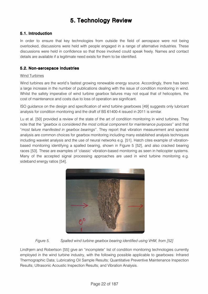
Lu et al. [50] provided a review of the state of the art of condition monitoring in wind turbines. They note that the “gearbox is considered the most critical component for maintenance purposes” and that “most failure manifested in gearbox bearings”. They report that vibration measurement and spectral analysis are common choices for gearbox monitoring including many established analysis techniques including wavelet analysis and the use of neural networks e.g. [51]. Hatch cites example of vibration-based monitoring identifying a spalled bearing, shown in Figure 5 [52], and also cracked bearing races [53]. These are examples of ‘classic’ vibration-based monitoring as seen in helicopter systems. Many of the accepted signal processing approaches are used in wind turbine monitoring e.g. sideband energy ratios [54].
Figure 5. Spalled wind turbine gearbox bearing identified using VHM, from [52]
Lindhjem and Robertson [55] give an “incomplete” list of condition monitoring technologies currently employed in the wind turbine industry, with the following possible applicable to gearboxes: Infrared Thermographic Data; Lubricating Oil Sample Results; Quantitative Preventive Maintenance Inspection Results; Ultrasonic Acoustic Inspection Results; and Vibration Analysis.
M A C H I N E R Y M E S S A G E
2Q04 ORBIT 61
DAMAGE ON THE INNER RACE OF ONE OF
THE INTERMEDIATE SHAFT SUPPORT
BEARINGS. THIS WAS ONE OF SEVERAL
SPALLS IN THE BEARING.
FIG. 3
0 50 100 150 200 250 300Frequency (Hz)
0.05
0
0.10
0.15
0.20
0.25
0.30
0.35
Am
plitu
de
Envelope SpectrumRaw Data Spectrum
Gear Mesh Frequencies
THE ENVELOPE SPECTRUM FROM THE MACHINE WITH
THE NEW BEARING SHOWS NO BEARING DEFECT
FREQUENCIES. THE RAW ACCELERATION SIGNAL
SPECTRUM (BLUE) IS COMPARED TO THE ENVELOPE
SPECTRUM (RED) OF THE OUTPUT SHAFT
ACCELEROMETER DATA. SEE ALSO FIGURE 2.
| FIG. 4
inner race ball pass (IRBP) frequency of one of theintermediate shaft bearings. It has two sidebandsthat are located at 8 Hz to either side of the 66 Hzfrequency. The next cluster of frequency lines cen-tered near 132 Hz represents harmonics of the grouparound 66 Hz. These harmonics are an artifact ofthe enveloping algorithm and have no physicalmeaning.The bearing was removed and inspected, and sub-stantial damage was found on the inner race. Figure3 shows one of several large spalls that were foundon this race.The bearing was replaced, and the wind turbine wasreturned to service. Data was collected again andprocessed as before. Figure 4 compares the raw accel-eration signal spectrum (blue) with the envelopespectrum (red) from the same accelerometer as inFigure 2. The spectrum of the raw accelerometerdata shows some gear mesh frequencies, but theenvelope spectrum is completely clean.
Conclusions
While the raw spectrum can be useful for moni-toring gear mesh frequencies, the envelope spectrumprovides superior sensitivity to bearing defect fre-quencies in wind turbine applications. The chiefadvantage of enveloping is that it provides excellentvisibility of bearing defect frequencies without thevisual interference of gear mesh frequencies in thesame spectrum. This effect can be seen in bothFigures 2 and 4, where gear mesh frequencies arepresent in the raw signal spectra but are absent inthe envelope spectra. This occurs because gearmeshing is a relatively smooth process and produceslittle impact energy. The gear mesh frequencies areremoved during the first high-pass filtering of theraw data.Enveloping thus provides a powerful tool for moni-toring wind turbine bearings. It is now included inour Trendmaster Pro System (see companion articleon page 20) as well as our Snapshot™ family ofportable data collection instruments. The result isenhanced capabilities for more proactive detectionof mechanical problems on these importantmachines.
Editor’s Note: You can read more about accelerationenveloping on page 10 in this issue of ORBIT.

Page 23 of 187
Hameed et al. [56] present a similar list, which includes for gearboxes: vibration analysis; oil analysis; strain measurements (noting that strain gauges are not robust, but fibre-optics might change this); and acoustic monitoring.
Lekou et al. [57] note that at present the wind turbine field uses oil analysis, debris monitoring and temperature monitoring alongside traditional vibration monitoring. Oil indicators include: oxidation, iron and copper concentrations; viscosity; colour; smell; and wear particle size [58].
In order to improve condition monitoring, Lekou et al. proposed an acoustic emission (AE) approach due to AE’s ability “to detect early pitting, cracking or other potential defects much earlier than the classical vibration method”. They presented results from AE sensors mounted on the gearbox casing which showed a correlation between the AE signals and the operating condition of the wind turbine.
In 2011 Dempsey [59], one of the key workers on HUMS at NASA, published work on health monitoring in wind turbines with Sheng from the National Renewable Energy Laboratory (NREL), showing that industrial crossover is taking place. In addition, in 2012, NREL conducted a round robin test of vibration processing algorithms [60], many of which were derived from helicopter HUMS.
In summary, a review of some of the relevant literature surrounding wind turbine condition monitoring yielded no new technologies of significance. This is perhaps unsurprising for such a mainstream industry; there are no significant aerospace technologies that have not been incorporated into the field nor any in the field that have not been carried over to the aerospace industry.
Formula 1
Gear and bearing failures in Formula 1 (F1) are not uncommon, and the safety systems are such that they are rarely catastrophic. However, given the points loss which accompanies a loss of drive, and the competition penalties imposed for changing gearboxes, there is considerable appetite to be able to predict impending failures. Therefore, work has been undertaken in the F1 industry into component monitoring.
However, discussions with a figure in that industry who has worked in transmissions for more than 5 years, suggest that this has not been successful to date. Whilst, a technology or capability could be hidden within a team, it is unlikely that it could have been kept completely secret for more than a few years.
The initial approach taken by some teams was to use vibration monitoring and drew on some of the available NASA papers for condition indicators. However, there were problems surrounding background noise, vehicle vibration and engine firing.
An alternative approach was used based on torque-sensing. Companies such as NCTE (www.ncte.com) and ABB (www.abb.com) supply shafts capable of measuring torque to the F1 industry. Such torque sensing shafts are already used in aerospace systems and are capable of operating in hostile environments and at very high shaft rotational speeds (e.g. >300°C and 20,000 rpm). See Figure 6.

Page 24 of 187
Figure 6. Torque sensing input shaft (from www.ncte.com)
However, in addition to torque sensors, Magcanica (www.magcanica.com) supplies rate-of-change (ROC) of torque sensors, which are used in connection with helicopter rotors, operating using magnetoelastic principles [62].
The theory in the F1 application was that discrepancies in torque would accompany a degrading gear and could therefore be sensed by an ROC sensor. However, they were unable to overcome the issues of noise, in particular the torque pulsation produce by the engine firing. The contact rightly noted that this may not be an issue in a gas turbine. Contact with the company showed that they are currently trying to apply the technology to helicopter HUMS [63].
Renaudin et al. [60] proposed a method for detecting faults in roller bearings by measuring the instantaneous angular speed through a pulse timing method. By taking a Fourier Transform of the signal, they were able to identify bearing spalls. However, the monitoring was carried out close to the faulty bearing. In order to monitor planetary gears in an epicyclic configuration, it would be necessary to mount directly to the planetary gear or planet carrier to monitor the rotational speed of the planetary gear about the planet carrier shaft. This would present many of the same challenges (e.g. data rate, power etc.) that face the more traditional technologies. In addition, the paper only presents results for single-row circular-roller bearings. It is unclear whether the same results would be obtained for double-row barrel-roller self-aligning bearings such as those used in the Super Puma gearbox.
Rail
Discussion with a rail contact showed that the rail industry uses condition monitoring for final drives, engines and engine-mounted gearboxes. The predominant technology is oil sampling, adopted by around two-thirds of the industry. They do not use acoustic emission, optical methods, or accelerometers although the latter was trialled and rejected. Typically, samples are taken around every 30 days.
! !

Page 25 of 187
Marine
The marine industry uses a variety of technologies for monitoring various components including monitoring gear meshing with accelerometers. For ships with thrusters (high throughput pumps), braking torques are used to monitor for blockages and prevent pump damage. Acoustic emission is used to detect liner scuffing. Finally oil debris analysis is used, in part because oil is shared between components and needs to be kept clean.
Military Land Vehicles
The use of sensors to monitor systems for the purpose of Health and Usage Monitoring in the fullest extent on military land vehicles is in general lower than in other fields. There are a number of sensors on board vehicles generally that monitor engine and gearbox information however these tend to be due to the fact that they are used for the commercial haulage market and are often not enabled for data collection. The Supacat Jackal vehicle (A high Mobility Weapons Platform currently in service) for example has a number of parameters that are available however as can be seen in Table 5 the information is largely not monitored.
There is a significant amount of data on the vehicle that could be utilised to a greater degree, however the current configuration only presents limited information to the user whilst driving and currently no further information is presented to the maintainer in the form of fault codes or HUMS output. As such any data that is collected from the vehicle for any onward usage is completed manually.
The main reason for the lack of use of HUMS in the Military environment is the result of a failure of any equipment is generally not life threatening (although it may be severely mission critical) and so cost becomes the main driving force. As such most land vehicle sensors are either direct feeds from aircraft sensors or are those that are cheap to manufacture accepting the possible degradation in accuracy that may be present. The main consideration for the fitment of aircraft type sensors however is that the land vehicle tends to experience less predictable and often harsher vibration profiles. The vast majority of sensors are already fitted to many parts of modern vehicles. They are particularly used by the engine management system to maintain good function throughout the vehicle
Military vehicles use both active and passive fault detection. An active approach involves transmitting clean signals through a component and measuring the response. Examples include the use of lambda waves for detecting crack propagation through thin sheet structures. The clean input signals make it easier to diagnose changes in the response. This approach requires transducers that emit the active signal as well as sensors to monitor the response and piezoelectric transducers are particularly useful because they can serve both roles.
Active methods are rarely used while the vehicle is operational so this method is better suited to those vehicles that return frequently to base. The approach is limited where heavily loaded components are concerned because it isn’t viable to provide on-board actuators that are capable of significantly stressing large components.

Page 26 of 187
Table 5. Military vehicle parameters to be monitored
Parameters
* Items Push data to either the CANbus or RS232
[*] = On CANbus / RS232 but not used
Data Available
Data Monitored
Data Collected and Processed with HUMS Unit
Suspension
On road setting selected* Y N N
Off road setting selected* Y N N
Maximum Displacement* Y N N
Minimum Displacement* Y N N
Acceleration 3 Axis Accelerometer N N N
Electrical Power
Vehicle Battery Voltage* Y Y N
Auxiliary Battery Voltage* Y Y N
BMS (Battery Management System) Contactor Status *
Y N N
Current (Auxiliary Battery Bank) N N N
Current (Vehicle Battery) N N N
Temperature
Engine* Y Y N
Ambient Y N N
Diff Cooler Operative * Y Y N
Gear Box * Y Y N
Engine / Gear Box
Fuel Usage * Y Y N
RPM * Y Y N
High / Low Range Selected * Y Y N
Selected Gear [*] Y N N
Throttle Position * Y Y N
Engine Torque [*] Y N N
Charge Air Temperature [*] Y N N
Time
Time Y N N
Mileage * Y Y N
Engine Run Hours [*] Y N N
The passive approach monitors data whilst the vehicle is operational. Examples include vibration monitoring of gearboxes to identify progressive faults. This approach is more suitable for heavily loaded components that require significant loads in order to measure a response. As passive monitoring takes place while the vehicle is operational it can be used to provide an instantaneous warning of failures. Examples of passive algorithms range from simple threshold monitoring of vibration and temperature levels to very complex neural network solutions for gearbox analysis.
Diagnostic techniques all rely on detecting the presence of a fault before it has time to cause serious damage. Components exhibiting this trait are known as ‘damage tolerant’ aside from a few

Page 27 of 187
transmission components, very few components on ground vehicles exhibit this trait. A number of experiments with ‘fatigue fuses’ have also been attempted on ground vehicles. These are sacrificial devices that are designed to monitor the same loads as a real component but fail in advance of the component thereby providing prior warning. These systems can be successful but are often expensive to design and implement and cannot be applied retrospectively to a component midway through its life.
Advanced technologies, such as those in Figure 7, are not necessarily new. But the availability of such technologies in highly reliable, miniaturized or micro-miniaturized form is new. The implication of such miniaturization for CBM is that more and more kinds of technology may be embedded in on-board operating weapon systems and used for condition-monitoring in real time.
Some technologies are more useful or more prevalent than others. For example, although not cited as an “advanced” technology, vibration monitoring is an important technology for condition-monitoring of equipment that contains rotating mechanisms or propulsion systems.
Figure 7. Generic CBM technologies

Page 28 of 187
5.3. Technology Review
This section details a review of existing and potential technologies for improving the monitoring of planetary gears and bearings. It begins by examining the fundamental physical mechanisms available for monitoring and then addresses specific technologies and concepts. Relatively little attention has been paid to acoustic emission and RFID sensors since these have already been identified by EASA as being of interest.
A number of organisations were approached to offer comments and suggestions about potential technologies and these include: UK AAIB, AIBN, ATSB, GE, USC, Airbus Helicopters, AugustaWestland, NASA and others. As with the non-aerospace industries, contributions will not be affiliated unless requested by the contributor.
The result of this process was a list of potential mechanisms, sensor types and placements to be carried forward to the next task (quantitative assessment), where performance and viability were addressed.
Sensing mechanisms
There are myriad references addressing mechanisms for condition monitoring, damage detection, condition-based maintenance etc. However, whilst no one source may be considered authoritative, most focus on a common core of mechanisms. Some of these are described below.
Dutta and Giurgiutiu [64] suggest a range of damage-detection technologies aimed at preventing catastrophic failure, listed as:
Passive and active scanning In-situ sensors
Ultrasonic probing Vibration monitoring
Eddy currents Strain monitoring (electrical and fiberoptics)
Liquid penetrant Peak-strain indicators
Thermography and Vibro-thermography Acoustic emission
Magnetic particles and Magnaflux Dielectric response
Computer tomography Emitter-detector pairs
Laser ultrasound Electro-mechanical impedance
Low power impulse radar
ISO issues general guidance on Condition monitoring and diagnostics of machines [65] which suggests the following relevant physical phenomena for condition monitoring: temperature; pressure; flow; input and output power; noise; vibration; acoustic emission; ultrasonics; oil pressure, consumption and tribology; thermography; torque; speed; length; angular position; and efficiency.
In 2012, Delgado, Dempsey and Simon of NASA [10] performed a review of rotorcraft engine health monitoring technologies highlighting vibration, oil debris monitoring and thermocouples as the main sensor types.
Sensor types
The types of sensors typically used for HUMS can be broadly grouped into (1) vibration, (2) strain-based (3) oil-condition and (4) temperature. Each group of sensors measures a different

Page 29 of 187
phenomenon exhibited when the component is behaving abnormally. Vibration-based sensors, typically accelerometers, detect fault patterns in the vibration signal when defects are present. Strain-based sensors do not directly detect defects, but monitor the applied loads on the component which cause the strain. Oil-condition based sensors, such as chip detectors, detect abnormally large particles in the lubrication oil when excessive damage occurs. Temperature-based sensors measure increased operating temperature arising from friction due to abnormal wear. The type of sensors used within each group may differ and they are discussed below. Other novel sensors that do not operate based on these four groups are discussed at the end.
5.4. Vibrat ion-based sensors
Accelerometers
The most commonly used vibration-based sensors in helicopter HUMS are displacement-based accelerometers and they are widely used for monitoring both rotor and drive-train systems. More recently, they are also used to detect faults in the planetary gears within the main transmission as well. For the rotor system, the accelerometers are used to monitor the ‘per revolution’ vibration level of the rotor blades where imbalance in the rotor blades will result in increased vibration. For the drivetrain system, the vibration signatures are processed and features or fault patterns are extracted to detect defects in the shafts, gears and bearings.
Applications in Helicopter HUMS
The survey will focus on cases where accelerometer sensors and their corresponding signal processing methods are applied in helicopter HUMS. Only cases where the HUMS application is validated through component seeded tests or field defects as mentioned above are considered. There are several commercially available HUMS system developed largely using accelerometer sensors. IMD-HUMS from Goodrich, ZING-HUMS (formerly known as IAC-HUMS) from Honeywell and EuroHUMS and MARMS from Eurocopter are some of the main HUMS program adopted by helicopter fleet today which installs several accelerometers on the rotor and drive-train system. Despite the wide use however, published literature on their performance in the field environment is limited. A survey of cases where fault detection was validated on a helicopter platform is shown in Table 6. It can be seen that all of the cases examined in this study were from military. From these cases, the most commonly adopted feature for bearing defects is the vibration energy at the bearing defect frequencies obtained from the FFT spectra. For gear defects, the FM4 feature was the most adopted feature that is obtained from the kurtosis of the residual vibration signal. The use of more advanced algorithms such as wavelet transform or use of artificial intelligence (AI) has yet to be demonstrated in the field environment.
Wireless Micro-Electro-Mechanical Systems (MEMS) accelerometers
In most of the applications for gearbox monitoring, including the cases above, the accelerometer is mounted on the gearbox housing. The noise level of the acquired vibration level can be high if the bearing or gear of interest is located deep within the housing and the signal is attenuated. In 2002, Abhijit et al. [66] proposed that MEMS sensors be embedded within a planetary gearbox and radio frequency (RF) be used to wirelessly transmit the vibration signals. This allows sensors to be placed on rotating parts within the gearbox without the need for complex slip rings. However, the work is largely theoretical and there was no actual testing of the proposed concept. Despite this, the concept is potentially viable, especially with commercially available wireless accelerometer sensors such as those developed by Microstrain®. The developed sensors have energy harvesters, as shown in Figure 8, which draws power from the vibration in the environment and does not require battery power.

Page 30 of 187
Aircraft Type
System Fault detection Analysis method
Feature Validation means
Ref.
AH64D Honeywell
Aft and Fwd Hanger Bearing wear, corrosion and lubricant contamination
Frequency Analysis
Bearing Energy
Seeded testing
[62]
AH64D Honeywell Main Swashplate bearing broken cage and spalling
Frequency Analysis
Bearing Energy
Field defect [19]
AH64D Honeywell Nose gearbox bevel gear
Time Analysis
FM4 Field defect [62]
AH64D Honeywell Tail Rotor gearbox bevel gear tooth crack
Time-Frequency analysis
- Seeded testing
[63]
AH64D Honeywell APU Clutch failure Time Analysis
Peak vibration
Field defect [19]
H-60 Goodrich Tail Rotor Bearing Frequency Analysis
Bearing Energy
Seeded testing
[64]
H-60 Goodrich Tail Rotor Gear scoring
Time Analysis
FM4 Field defect [62]
H-60 Goodrich Main gearbox Bevel Gear coating anomaly
Time Analysis
Residual Kurtosis
Field defect [62]
H-60 Goodrich Hanger Bearing Frequency Analysis
Bearing Energy
Seeded testing
[64]
H-60 Honeywell Oil Cooler Fan Bearing spalling and pitting
Frequency Analysis
Bearing Energy
Field defect [65]
H-60 - Planet gear carrier fatigue crack
Time Analysis
FRMS1, NSDS2
Seeded testing
[66]
AS332 Eurocopter Tail Driveshaft double Bearing spalling
Frequency Analysis
Bearing Energy
Field defect [67]
OH-58 - Main gearbox input pinion tooth crack
Time Analysis
FM4 Seeded testing
[68]
CH-47 Honeywell Main rotor swashplate bearing
Frequency Analysis
Bearing Energy
Seeded testing
[69]
1: Filter Root Mean Square; 2: Normalised Sum of Difference Signal
Table 6. Cases of Helicopter HUMS application using accelerometers
!

Page 31 of 187
The size of the harvester is proportional to the data sampling rate required and can be reduced to considerably small sizes. In [67], such Microstrain® sensors were installed and flight tested on an MH-60S helicopter. Notably, these sensors have been qualified to airworthiness requirements such as MIL-STD-461F for electromagnetic interference and compatibility [68]. However, the ability of these sensors to withstand the high temperature and lubricant laden conditions within the gearbox would require further evaluation. Furthermore, the risk of the sensors dislodging within the gearbox and becoming a foreign object damage (FOD) debris is a critical safety consideration.
Figure 8. MicroStrain’s vibration energy harvester from [69]
More recent work has been carried out by AgustaWestland into the use of energy harvesting HUM systems [70].
Similar to this sensor is the Prognostic Integrated Multi-Sensor MEMS Module (PRISM) shown in Figure 9. This sensor integrates many of the sensing elements required for effective system life tracking within a small, single device. The PRISM is a “near-penny-size” sensing system based on MEMS technology for measuring temperature, relative humidity and vibration/shock. This can be extended to include strain. The project goal is to create a full sensing system – including all associated analog-to-digital conversion electronics on board
This technology was predicted to be at TRL 6 in early 2013 with helicopter trials planned. In early 2012, the manufacturer of the PRISM sensor, Impact Technologies was bought by the Sikorsky Aircraft Corporation.
Figure 9. PRISM sensor (from www.impact-tek.com)

Page 32 of 187
One solution is offered by Brüel and Kjær, an instrumentation and measurement manufacturer. The system is a vibration sensor capable of operating: in harsh environments, at temperatures up to 160˚C; without physical power connection (i.e. battery or other power source); and without a physical communication connection (wireless). This is a Bluetooth solution operating at 2.4 GHz using inductive power transfer.
Figure 10. Sensing and transfer components of Brüel and Kjær wireless accelerometer
Figure 10 shows the necessary components attached to an engine con-rod and a bracket for attaching the induction coil in the engine sump. The size and weight of this system is considerable, particularly the inductive coil required to transmit power.
MicroStrain produce a sensor called the EmbedSense wireless sensor (see Figure 11).
Figure 11. MicroStrain EmbedSense wireless sensor
The node uses an inductive link to receive power from an external coil and to return digital strain, temperature and unique ID information. A reader coil is energized by an AC electromagnetic field from a 125 kHz signal supplied by the reader unit. The embeddable node is 36 mm (diameter) x 7 mm (height) and can withstand temperatures of -40 °C to +125 °C. Typically a gap of around 50mm can be crossed by the wireless technology.
Acoustic Emission
The use of acoustic emission (AE) sensors is much more recent compared to the use of accelerometers for fault detection. Although it is not a typical vibration-based sensor, it is discussed together as the signal processing methods are similar. Unlike displacement-based accelerometer sensors, AE sensors detects stress wave that propagates through the material when crack surfaces
Produced modules
Box contains:
• Switch mode PSU
• Buck converter
• Pulse generator
• Receiver board
Inducer coil housing, containing:
• Inducer coil
www.bksv.com, 8
• 2.4GHz antenna
• Heat sink.
• Mounted on Crank bearing bracket.
Conrod module:
• Pick up coil
• 2.4GHz antenna
• 2.4GHz Transmitter
• Transmitter PCB bracket

Page 33 of 187
are formed. As the crack propagates, the frequency of the stress wave increases and these activities are monitored by the AE sensor. As such, AE is suitable for detecting early stages of crack initiation. Besides early detection, use of multiple AE sensors also allow defects to be located by using the time delay in the signals between the sensors. There are several works showing the feasible use of AE sensor for detecting failures in drive-train components such as shafts [71], bearings [72] and gears [73]-[75]. In these works, various time and frequency domain analysis methods were also applied to extract features for fault detection. This research into the monitoring of the gearbox however, is confined to testing in the laboratory and involves the use of slip ring for the acquisition of the AE signal from rotating components. In practice, such installation of AE sensors on the helicopter may be too complex. From this survey, there are currently no published works on the use of AE sensors on helicopter HUMS found nor was there any testing on a helicopter test rig. As such, the performance of AE in a complex gearbox with noisy environment has yet to be evaluated.
Wireless Acoustic Emission Sensor
The use of wireless technology may mitigate the complexity of installing the AE sensor within the gearbox. The use of piezoelectric wafer active sensor (PWAS) based wireless AE sensor has been developed as described in [76]. Like the energy harvesting sensors mentioned above, these AE sensors do not require a battery and can be installed in-situ on different rotating components for higher signal-to-noise ratio performance. The work is still developmental in nature but can potentially be commercially viable and qualified to airworthiness requirements like the wireless sensors developed by Microstrain®. The signal processing required for AE detection would require some attention since it tends to use parameters such as: amplitude, energy, counts, duration, rise time, counts to peak, average signal level, energy index etc.
Alternatively, the PWAS sensor, which is an output of laboratory for active materials and smart structures at the University of South Carolina with whom we have been in contact, can be used in an impedance mode to detect defects e.g. [64]. A similar product is the macrofibre composite (MFC), which is a flexible piezoelectric transducer from Smart Material (smart-material.com). This type of transducer could be fitted to curved structures such as between the inner race of the bearing and the planet carrier. This can also act in a power-harvesting role.
In addition, Smart Material also manufacture PZT fibres (105µm, 250µm or 800µm diameter) which could be embedded into or wound around structures.
5.5. Strain-based sensors
As the MFC patches above indicate, there is not a clear distinction between ‘vibration’ and ‘strain’ measurement.
Wireless strain gauge
Strain gauges have been traditionally used to measure loads in instrumented flights on helicopters. However, the challenge of installing sensors on rotating components restricts load monitoring to largely stationary parts such as the helicopter mast. Yet again, the use of wireless MEMS based sensors has allowed this to be overcome. Arms et al. [67] demonstrated a wireless strain sensor from Microstrain® which was installed and flight tested on the pitch link of the MH-60S helicopter as shown in Figure 12. This allows the structural loads of the pitch link to be monitored and its fatigue life to be accurately assessed based on usage.

Page 34 of 187
Figure 12. Wireless strain sensor installed on the MH-60S pitch link from [69]
Optical fibre strain sensor
Optical fibre strain sensors work based on the principal that the wavelength of the reflected light changes according to the induced strain on the optical fiber. The use of optical fibre strain sensors for structural health monitoring is gaining popularity due to their light weight, wiring simplicity for multiple sensors and immunity to EMI/EMC compared to traditional strain gauges. In [77], NASA applied the use of optical fiber strain sensors to diagnose defects in the OH-58 planetary gearbox test rig. In that work, the optical fiber sensors were installed on the stationary ring gear and the gearbox housing had to be modified to accommodate the transmission path of the fiber. The acquired time-series strain data from the sensors showed very high repeatability with high signal-to-noise ratio compared to the conventional accelerometer based measurements. They then applied time domain analysis methods (used in accelerometer based time series signal) to the strain data to diagnose for fault patterns. They concluded that the technique is effective in detecting planet gear cracks and spalls but has limitations in detecting defects in the sun gears and bearing races located deeper within the gearbox. Notwithstanding its benefits over conventional accelerometers, optical fiber strain sensors requires a transmission path and cannot be suitably applied to monitor rotating components.
Magnetic stress sensors
Magnetic stress sensors operate based on the principle that the magnetic permeability of a ferromagnetic material changes as it is subjected to mechanical loading, also known as the inverse magnetostrictive effect. The key advantage of this technique is that it does not require contact with the component it is monitoring. In [78], a JENTEK Quadri-Directional Magnetic Stress Gage (QD-MSG™) was used to monitor applied torque, axial and bending loads on a rotating shaft as shown in Figure 13. Both static test and dynamic tests were carried out with the latter performed under different torque loading conditions. It was shown that this approach can accurately obtain the applied torque loading after the measurements are corrected for hysteresis and temperature effects. As this method is contactless, it is ideal for installation on existing helicopter platforms. It can also be applied on non-ferromagnetic components by using a ferromagnetic coating on them. However, due to its magnetic based operating principle, it may have challenges when applied to areas on the helicopter where EMI/EMC is critical or where magnetic interference is high.
This is the same technology as highlighted by the F1 contact, albeit without the rate-of-change information.

Page 35 of 187
Figure 13. Magnetic Stress gauge array installed around the rotating shaft from [78]
5.6. Temperature sensors
Temperature can be an extremely useful parameter to monitor, sometimes giving indications of problems before physical damage occurs.
Thermocouple
The use of thermocouples to monitor temperature within gearboxes and engines is well-established and is widely used to provide temperature exceedance warnings. In most cases, the temperature of the lubricant or ambient air in the gearbox provides an indirect measurement of the gears and bearings temperature, which can heat up in the presence of abnormal wear and damage. In a grease leak test performed on the AH64 tail rotor gearbox [79], it was shown that the actual gear temperatures are much higher than the ambient temperatures measured at the gearbox’s thermistor locations as shown in Figure 14. The high temperature gradient between the gear mesh and the thermistor location meant that the overtemp will only be detected later. As mentioned in [79] also, the temperature limit is seldom exceeded but when it is, it can be very rapid and instantaneous. As such, in-situ monitoring of the bearings and gear temperature itself can provide earlier warning of incipient failure. The complexity of mounting sensors on the rotating parts however remains a challenge.
Figure 14. Infrared image showing high temperature gradients on gearbox surface from [79]
Advances in technology have produced extremely small thermal imaging cameras, such as the one shown in Figure 15, manufactured by Thermoteknix Systems (thermoteknix.com). Such cameras are small, light and draw little power and this model is capable of 60 frames per second (fps), others can achieve 120 fps. A monitoring solution may be possible which utilises high speed themal imagery of the gears directly rather than of the gearbox casing.

Page 36 of 187
Figure 15. Small thermal imaging camera (from thermoteknix.com)
Direct thermographic monitoring such as this is already achieved for open gears in operation as shown in Figure 16.
Figure 16. Thermographic monitoring of open gears [from sirfrt.com.au]
Wireless MEMS thermocouple
Similar to vibration-based sensors above, MEMS-based thermocouple sensors can potentially provide a wireless solution to eliminate the need for complicated wiring on the helicopter. A small yet robust wireless MEMS temperature sensor was developed and tested on a bearing cage to temperatures in excess of 300°C [80] as shown in Figure 17.
!
Open Gearing
Open gearing allows thermography of gears directly while in service. The prime function of using thermal images in this application is for monitoring the effectiveness of gear tooth lubrication. Lubrication is usually by grease, often applied by grease sprays. Uneven or inadequate application of grease causes an increase in temperature or variations in temperature patterns across the gears. Misalignment of gears is a much more likely problem with open gearing as alignment is usually a manual on-site setup, compared to gearbox where accuracy is controlled in a manufacturing environment. Again variation of temperature across the gear is the observed misalignment symptom. A common application for open gearing is for rotating crusher drums or rotary kilns. The larger gear is often assembled in segments around the drum or kiln and this gives the possibility of setup variation in gear tooth contact between the different segments which can be detected by temperature around the gear.
Conclusion The cost of a basic level Thermography camera is low enough to allow use by the average maintenance person who has responsibility for inspection or condition monitoring of equipment. This article presents some opportunities for use of the technology with gearboxes and gearing. The application of thermography for inspecting equipment is so broad that it will become much more widespread and basic thermography condition monitoring knowledge and skills will become a basic requirement of maintenance people involved with inspecting equipment.
By Peter Todd – Facilitator NSW Industrial Maintenance Roundtable working for SIRF Roundtables
Source of images used in this article are Erik Thorup, Leith Hitchcock and Flir Systems

Page 37 of 187
Figure 17. MEMS temperature sensor integrated onto a bearing cage from [80]
The sensor can identify changes in its resonant frequency as the temperature changes and has good linear performance. In addition, there is constant sensitivity in its measurement throughout the entire temperature range. The test however was performed on a static bearing cage and its performance in an actual gearbox was not evaluated.
5.7. Oil condit ion sensors
Spectrometric oil analysis
Spectrometric oil analysis is a technique used to determine the type and amount of metallic wear as indicated by the oil condition. Oil samples from within engines and gearboxes are regularly taken and sent to a laboratory where atomic emission spectrometer or atomic absorption spectrophotometer determines the type and concentration of particles in the oil [81]. The presence of high concentrations of a particular element type can indicate abnormal wear of a component and can also be used to detect contamination when elements foreign to the gearbox are detected. By tracking the concentration of the wear particles, the damage progression of the components can be monitored with the approach being well-suited to monitoring slow wear progression. However, large wear debris such as chips and cracked gear teeth cannot be detected using this approach. As a laboratory is usually required to perform the assessment, this can generally only be carried out off-line. Nonetheless, spectrometric oil analysis is widely practiced in military fleets such as monitoring the main gearbox of the Canadian Forces Sea King helicopter [82].
Magnetic debris detection
Magnetic chip detection is the most common oil-condition sensor used on helicopter gearboxes and engines. It is located downstream of critical component and detects failures when the debris from worn components are collected in the lubricant. It typically consists of a magnetic plug-type filter with electrical contacts that is closed when sufficient metallic debris is accumulated across it to provide a caution indication. These filters are also periodically inspected during scheduled maintenance to check for abnormal accumulation of debris. As there can be significant amounts of wear debris even in the normal operation of the gearbox, the threshold to detect abnormal wear is typically set much higher to avoid high false alarm rates. In more recent magnetic chip detectors, accumulation of fine particle across the contacts are burned off to reduce such false alarms. Magnetic chip detection is unable to isolate the defective component as it can be triggered by any metallic debris.

Page 38 of 187
Inductance type debris detection
Inductance type debris detection is more recent than both spectrometric oil analysis and magnetic debris detection and has advantages over both methods. Like the magnetic debris detector, the inductance type debris detector is located downstream of critical components and detects debris in the lubrication fluid. However, it detects debris based on the disturbance of a magnetic field by the passage of a metallic particle. The disturbance of the magnetic field induces a voltage in a sensing coil and the amplitude and phase of the voltage can be used to determine the type and size of the particle [83]. It can provide on-line sensing and can detect and distinguish small wear particles. This technology has already been developed by Goodrich and GASTOP for application on the AH64 helicopter [84] and F22 aircraft [83]. In a related study, the use of this method to detect fatigue damage in spur, bevel gears and bearings was tested using NASA’s Glenn 500-HP gearbox fatigue test rig [85]. Based on the statistical distribution of the particle count, it was concluded that the method is effective in detecting gear and bearing damage but is unable to distinguish between the two when both share a common lubrication system.
This is an active subject of considerable research effort by NASA and the US Army e.g. [86].
5.8. Other sensor types
Comparative Vacuum Monitoring
Comparative vacuum monitoring (CVM) [87] is a new monitoring technique developed by SMSYSTEMS that works based that a vacuum maintained within a small volume is sensitive to any leakage. As such, a polymer based sensor with adjacent rows of air galleries embedded as shown in Figure 18. This sensor is bonded onto fatigue critical locations across the crack propagation path and a vacuum is maintained in the sensor galleries. When a crack develops on the structure, air leaks through the crack into the gallery. By tracking the galleries with leaks, the crack length can be determined. As with optical fiber sensors, it is lightweight, immune to EMI/EMC effects but requires a transmission path for the vacuum to be maintained in the galleries. As such, it is not suitable for rotating components but can be used to monitor stationary structures such as the gearbox support instead. As the sensors are sensitive to leakage, they have to be bonded carefully else false alarms arising from dislodged sensors may occur.
Figure 18. Crack detection using comparative vacuum monitoring from [85]
Acoustic measurement
NASA published a considerable body of work in the field of gearbox noise [88]-[91]. The original aim of this work was to model and predict noise from gearboxes with the intent of reducing noise.

Page 39 of 187
However, it is feasible that by understanding and predicting the noise that a gearbox should generate under given torque-loading conditions, it may be possible to identify anomalies. The most compelling evidence that this may be possible comes from the AAIB report into the accident to G-REDL which, when discussing the CVR recording of the cockpit area microphone (CAM), comments that:
“Three minutes and 24 seconds prior to the MGB oil low pressure warning, an amplitude step change was identified at harmonic frequencies matching those which may be observed in the case of second stage ring gear damage.”
Of course, this was indicative of a large impending or ongoing failure; more subtly damage may not be so easily detected. Atherton, Pintz and Lewicki [92] presented results of automated acoustic intensity measurements on spur gears. These showed that tooth profile had a major effect on the measured noise and that load and speed also affected the noise. Oswald et al. [88] demonstrated predictions of spur gearbox noise that agreed to typically within 3 dB (average 2.4 dB) of measured values. Work was carried out by NASA in 2012 [93] aiming to predict the vibro-acoustic interaction and radiation of gearbox noise.
Monitoring could be achieved by a single microphone, which would offer limited possibilities, or by using an array of microphones, possibly mounted within the gearbox, coupled with advanced signal processing. This could offer a measure of acoustic intensity (a vector with direction rather than sound pressure level which is a scalar), or even facilitate nearfield acoustic holography e.g. [94].
Ultrasonic inspection
The use of ultrasonics to inspect parts is long established in the field of non-destructive testing. In general, it is used as an active technology with ultrasonic waves being sent into a component and the reflection being monitored for time delay and amplitude change. It may be possible to mount ultrasonic sensors directly onto planetary gears, however, in all likelihood they will only provide useful information when the engine is not running; the ‘noise’ of the running gearbox will most likely swamp any ultrasonic signal introduce into the gear. Recent work has speculated on the possibility of non-contact detection of damage [95].
X-Ray computed tomography (CT)
CT scanning has seen significant growth in recent years in a variety of fields, including accident investigation. Using multiple 2D X-ray ‘slices’ a 3D picture can be built up of components making it ideal for an application such as detecting defects. However, the equipment is large, requires considerable power and often requires large doses of radiation making it unsuitable for real-time monitoring.
Laser scanning
Mounting a laser such that it can access the interior of the gearbox could provide a measuring solution. Laser beams can provide high levels of accuracy and are therefore often used in coordinate measuring machines (CMMs) which can provide accuracy to the micron level. Lasers are also finding greater use as range finders and small lightweight measurement devices measuring distances by reflecting from objects. However, as is often the case, accuracy is generally at odds with low cost, weight and size and it is unlikely that the accuracy required to measure physical discrepancies such as, say, pitting, could be achieved in an acceptable package. In addition, real-time measurement is unlikely to be possible to an acceptable level. Oil on the surface would disrupt the laser and finally, only ‘exterior’ surfaces would be available.
!

Page 40 of 187
Photography / video / photogrammetry
As with laser scanning, high resolution imagery may be able to provide an insight into gear condition but real-time monitoring is unlikely to be possible and only exterior surfaces of a planetary gear would be available. However, in combination with other techniques, imagery and/or laser scanning could be configured to provide views of planetary gear surfaces when stationary without dismantling the gearbox. Alternatively a series of fast shutter speed images, or high speed video, taken from a camera looking into the gearbox through a lens or transparent section could provide useful information, although oil contamination of both the lens and gears will be an issue. An additional issue will be getting full sight of the gears – the ideal position would be looking through the ring gear although this is not practical. High speed imaging at 1000 fps is achievable.
Luminescence
Dye penetrant inspection is an established NDT technique. Combining imagery as described above with lighting and a luminescent additive in the gearbox oil might allow improved imaging of cracks and damage. This will suffer from the restrictions mentioned above for imaging.
Fusion
As mentioned previously, combining complementary technologies can improve detection strategies and offer a more detailed insight into problems. However, these must be independently robust otherwise the net effect can be worse rather than better. As such, data fusion will only be considered once independent technologies have been established, rather than aiming to combine at too early a stage. The fusion of vibration and oil debris data is a major research theme for NASA and the US Army.
5.9. Conclusions and candidate technologies:
There are very few totally “new” sensing technologies; the majority of novel technologies utilize long-established principles but take advantage of developments in materials, processes, size, cost etc. to apply them to new areas of interest.
Accordingly, this review has found no fundamentally new physical mechanisms or technologies with which to detect incipient failures in planetary gears and bearings. However, it has taken a fresh look at novel potential approaches for monitoring planetary gears and bearings. Some of these will be deemed infeasible due to practical limitations, whilst others will be considered too insensitive. The assessment of suitability will be discussed in the next Chapter.
Table 7 presents some of the possible technologies with comments regarding their implementation.
! !

Page 41 of 187
Physical Mechanism
Placement Comments / Issues
Vibration
Mounted to gear body Space and mounting mechanism crucial.
Wireless data link
‘Smart bearings’ (sensing components perform functional role)
Compromise bearing strength?
Sensing layer (MFC or similar between planet carrier and bearing inner race
Signal could be routed to multiple senders on planet carrier body
Inside hollow planet carrier Compromise planet carrier strength? Signal
sending as above
Outside of gearbox Current HUMS system
Strain
Most of the locations and comments for vibration can be extended to strain
Embedded fibre optic Compromise gear strength?
Torque sensing of shaft(s) Sensitivity for gear / bearing damage?
Temperature
Embedded thermocouple e.g. bearing cage. Wireless offload required.
Thermal imaging video Oil contamination of lenses and parts.
Rotating parts will need very fast shutter or high-speed video.
Acoustic Inside gearbox
Holes in casing only needed (wireless transmission not necessary)
Transmission deck Useful supplement to other technique?
Comparative vacuum
monitoring Structure Not suitable for rotating components
Ultrasonics Mounted to planetary gears Stationary only?
Imaging / video
Line of sight (including mirrors) to component of interest
As with thermal imaging
X-ray Inside gearbox Size, power, radiation
Dye penetrant inspection
Inside gearbox Stationary only, limited view
Table 7. Potential technologies for planetary gear and bearing monitoring (not exhaustive)

Page 42 of 187
6. Technology Select ion
6.1. In i t ia l sort
This Chapter aggregates the new solutions discussed previously and begins an initial sort process to identify candidate technologies for direct component monitoring of MGBs.
6.2. Aggregated solut ions
Table 8 reproduces and expands on the solutions identified in Task 1 of the project, described in the previous Chapter, including the use of microelectromechanical systems (MEMS) sensors. Some include specific installation detail whereas others are more general concepts.
Number Physical
Mechanism Potent ia l Placement
Posit ion Comments / Issues
01
Vibration
MEMS mounted to gear body Space and mounting mechanism
crucial. Wireless data link
02 MEMS mounted to planet carrier Potentially more space and power opportunities. Wireless data link.
03 ‘Smart bearings’ (sensing
components perform functional role)
May compromise bearing strength
04 Sensing layer (MFC or similar)
on or between planet carrier and bearing inner race
Signal could be routed to multiple senders on planet carrier body
05 Outside of gearbox Current HUMS system
06
Strain
MEMS mounted to gear body As for vibration (01)
07 MEMS mounted to planet carrier As for vibration (02)
08 Embedded fibre optic or similar Compromise gear strength?
09 Torque sensing of shaft(s) Sensitivity for gear / bearing damage? Not proven for epicyclic gear stages
10
Temperature
MEMS mounted to gear body As for vibration (01)
11 MEMS mounted to planet carrier As for vibration (02)
12 Embedded thermocouple e.g. bearing cage. Wireless offload
required.
13 Thermal imaging video Oil contamination of lenses and parts.
Rotating parts will need very fast shutter or high-speed video.
!!!!!!
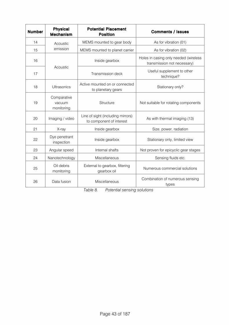
Page 43 of 187
!
Number Physical
Mechanism Potent ia l Placement
Posit ion Comments / Issues
14 Acoustic emission
MEMS mounted to gear body As for vibration (01)
15 MEMS mounted to planet carrier As for vibration (02)
16
Acoustic
Inside gearbox Holes in casing only needed (wireless
transmission not necessary)
17 Transmission deck Useful supplement to other
technique?
18 Ultrasonics Active mounted on or connected
to planetary gears Stationary only?
19 Comparative
vacuum monitoring
Structure Not suitable for rotating components
20 Imaging / video Line of sight (including mirrors)
to component of interest As with thermal imaging (13)
21 X-ray Inside gearbox Size, power, radiation
22 Dye penetrant
inspection Inside gearbox Stationary only, limited view
23 Angular speed Internal shafts Not proven for epicyclic gear stages
24 Nanotechnology Miscellaneous Sensing fluids etc.
25 Oil debris monitoring
External to gearbox, filtering gearbox oil
Numerous commercial solutions
26 Data fusion Miscellaneous Combination of numerous sensing
types
Table 8. Potential sensing solutions
! !

Page 44 of 187
6.3. In i t ia l sort
Some of the technologies above, whilst offering some potential, are considered to be inappropriate once the specific application is considered. Therefore, an initial sort is given below, aimed at eliminating those technologies which will not be considered further.
22 - Dye penetrant inspection
This technology could only realistically be expected to provide a useful measure of condition when the gearbox is stationary. However, the project has a clear requirement to monitor the gearbox in-flight.
Rejected as a stat ic measure
19 - Comparative vacuum monitoring
Whilst useful for monitoring structures this technique holds too many difficulties for practical implementation within a gearbox.
Rejected based on pract ical considerat ions
21 - X-ray CT
CT scanning offers an excellent analytical tool, but the power, weight, access and controls required mean that it is not yet practical for fitment to aircraft. In addition the risks posed by a radiation source may outweigh the benefits offered.
Rejected based on power requirements and radiat ion safety issues
24 - Nanotechnology
In this context, nanotechnology is taken to mean concepts such as pressure-sensitive oil additives. In general, many of the more ‘exotic’ nanotechnology solutions are in development and are simply not at a technology readiness level that will support testing. However, the manufacture of micro and nano scale sensors is much better developed and shows considerable potential (see Section 6.5).
Specif ic sensor solut ions carr ied forward
18 - Ultrasonics
There have been suggestions that by using say, a stream of oil as a coupling medium, ultrasonic energy can be sent to and received from a component such as a planetary gear. Such a system may allow in-situ, ultrasonic non-destructive testing (NDT) to be performed. However, there is a subtle distinction between employing an active system (which inserts energy and monitors returns) and a passive system (which only receives energy generated from processes within the component). Because of the high level of rotational noise, the energy that would be required from an active device in order to exceed the background noise would be excessive. However, the high energy level from rotation can be exploited by passive sensors.
Act ive ultrasonics is rejected due to energy requirements and noise, passive ultrasonic sensing is carr ied forward as acoust ic emission / h igh frequency strain
!

Page 45 of 187
03 - Multifunctional components
The accident to G-REDL highlights the stresses placed on compound planetary gears, and the complexity involved in producing reliable components. Therefore, incorporating any sensing technologies into load-bearing components (rollers or bearing faces) will only compound the issues already being faced.
Sensing rol lers and faces rejected
12 – Embedded thermocouple in bearing cage
The use of a bearing cage to carry a thermocouple is a novel use of a non-structural bearing component. However, a very similar effect can be achieved by applying temperature sensors to the bearing race, which for the stationary race adds the advantage of knowing the sensor location.
Not carr ied forward as a similar effect can be achieved more simply
08 – Embedded strain gauges
As described in the first report, NASA used optical fiber strain sensors embedded in the ring gear to diagnose defects in the OH-58 planetary gearbox test rig [77]. In that work, the strain data from the optical sensors shows very high repeatability with high signal-to-noise ratio compared to the conventional accelerometer based measurements. They concluded that the technique is effective in detecting the planet gear cracks and spalls but has limitation in detecting defects in the sun gears and bearing races located deeper within. Therefore, in order to get better defect detection, it would be necessary to embed the gauges closer to the planetary gears, and most probably in the planetary gears. As describe above (03), this is very likely to induce weakness in the component and therefore compound any difficulties being encountered.
This technology wi l l not be carr ied forward for th is study but is left open for continuous monitor ing as the technology develops
25 – Oil-based debris sensors
Oil-based debris sensors such as metallic chip detectors are already used widely in helicopters as a discrete health indicator of the gearbox. As it is based on detecting the wear debris in the oil, this technology does not suffer in fault detection performance from the increased complexity of a planetary gearbox. An online inductance type oil debris monitoring system has already been developed by Goodrich and GASTOP for application on the AH64 helicopter [84] and F22 aircraft [83] and this is an area of considerable study for NASA. As a result, any small-scale testing or development work considered under this project would be redundant.
Commercial ly avai lable and subject of considerable research effort - not considered further
26 – Data Fusion
The focus of this research is to improve the fault signal available to a detection algorithm. Whilst fusion might offer improved detection [59] [96], it is nonetheless a data processing approach and as such will benefit from improved signal levels. Therefore, fusion per se will be discounted for the current study although the potential of utilising information from multiple sensors will be retained.
Kept open, but not the focus of th is work

Page 46 of 187
09 & 23 – Torque rate of change and optical speed
Work has been carried out [63], Error! Reference source not found. to demonstrate the use of rate-of-change of torque and shaft speed in detecting gear and bearing problems. However, the technique is still developing and there is no evidence that it will provide useful information for epicyclic stages. Also, it will suffer from similar data and access constraints to the other solutions. Despite this, it might provide useful information in the future, particularly regarding shafts and simple gear setups.
No proven signif icant advantage over other technologies, but could be incorporated in later i terat ions
13 & 20 – Imaging / Video / Thermal imaging
Whilst the use of imaging techniques may lend a level of confidence to an operator, there are severe limitations to their use in a dynamic gearbox. Oil contamination of the lens and coating of the component will restrict optical access. Also, detecting some of the failure modes of interest may be impossible using standard visual means – crack and defect sizes that are detectable visually, might be considered to be too significant to be allowed. Finally, considering the G-REDL case study, obtaining visual access to outer bearing race of the planetary gear would be extremely difficult, if not impossible. For this reason, visual techniques are rejected.
Rejected based on inabi l i ty to detect in G-REDL case study
05 – External accelerometers
This is the configuration of current HUMS systems, and since no significant improvements can be proposed, this will not be discussed further. Clearly existing HUMS systems can be retained if they offer benefit.
No further discussion
Given this initial sort, Table 8 is reduced to those solutions given in Table 9.

Page 47 of 187
Number Physical
Mechanism Potent ia l Placement
Posit ion Comments / Issues
01
Vibration
MEMS mounted to gear body Space and mounting mechanism
crucial. Wireless data link
02 MEMS mounted to planet carrier Potentially more space and power opportunities. Wireless data link.
04 Sensing layer (MFC or similar)
on or between planet carrier and bearing inner race
Signal could be routed to multiple senders on planet carrier body
06 Strain
MEMS mounted to gear body As for vibration (01)
07 MEMS mounted to planet carrier As for vibration (02)
10 Temperature
MEMS mounted to gear body As for vibration (01)
11 MEMS mounted to planet carrier As for vibration (02)
14 Acoustic emission
MEMS mounted to gear body As for vibration (01)
15 MEMS mounted to planet carrier As for vibration (02)
16 Acoustic
Inside gearbox Holes in casing only needed (wireless
transmission not necessary)
17 Transmission deck Useful supplement to other
technique?
Table 9. Solutions carried forward from initial sort

Page 48 of 187
6.4. Operat ing restr ict ions
This section will review the MGB environment in order to establish baseline operating requirements for any proposed sensors. Precise conditions differ on each platform and so in general a ‘worst case’ assessment will be used.
Connection constraints
Clearly the rotation of the gearbox means that if wired signals are to be carried from inside the gearbox to outside the use of slip-rings or a similar system will be required. This is considered impractical for a range of reasons including mechanical complexity and space. Therefore, only technologies which allow data to be transmitted wirelessly will be considered.
Space constraints
There are two key aspects when considering space constraints within the gearbox. The first is mounting location, and the second is clearance.
In order to gain maximum signal, it is important for the defect signal transmission path to be as short / direct as possible since material losses and geometric spreading (see Section 6.5) will tend to reduce signal levels. Therefore a location should be found that is close to the point of interest (in the case of G-REDL, the planetary gear bearing) with sufficient contact area for the sensor to work effectively and sufficient clearance for the sensor to rotate with the gear and/or planetary carrier.
With that in mind, considering a second stage planetary gear (see Figure 19), such as that which failed in the accident to G-REDL, there are two flat surfaces available at the top and bottom of the gear which form part of the outer bearing race and the inner bearing race. The flat areas are approximately 10mm and 7mm wide respectively. The planet carrier shaft (see Figure 20) which runs centrally through the inner race is approximately 55mm diameter. There is no relative motion between the inner race and the carrier shaft, but clearly the outer race rotates relative to the carrier shaft.
Figure 19. Second stage planetary gear

Page 49 of 187
Figure 20. Second stage planetary gears and carrier from [1]
The clearance available between the second stage gear and the second stage planetary carrier and between the second stage gear and the first stage planetary gear carrier is extremely small, being of the order of centimetres at most. This significantly restricts the type of sensors that can be attached to a second stage planetary gear in this particular gearbox configuration. However, the tight clearances between carrier and casing may make wireless offload easier.
Figure 21. Sectioned EC 225 gearbox (taken from Eurocopter video)
Figure 22 shows a schematic of the S-92 gearbox. This also contains multi-level epicyclic and as such shares similar space constraints with the Super Puma gearbox above.
51
Air Accident Report: 2/2011 G-REDL EW/C2009/04/01
© Crown Copyright 2011 Section 1 - Factual Information
attached to the planet carrier but the gear / outer raceway and its associated bearings and bearing cages had separated from the inner race. Three sections of this gear were recovered, identified as the 9-tooth, the 10-tooth and the 16-tooth section, (see Figure 23). In addition, 12 of the gear’s 28 bearings were recovered.
Figure 22Complete undamaged gear, for reference
Figure 21Second epicyclic stage, as found (shown inverted)

Page 50 of 187
Figure 22. S-92 main rotor gearbox layout from [98]
In addition, it may be necessary to balance any rotating components by mounting additional sensors or dummy masses in opposing positions.
Temperature constraints
The AW139 Quick Reference Handbook (QRH) gives the acceptable operating range of MGB temperature to be from 1˚C to 110˚C and with a minimum startup temperature of -40˚C.
For an S-92, the ‘red zone’ of main gearbox temperatures begins at 130˚C [98].
The Flight Manual for the SA 330J gives a maximum operating temperature of 125˚C, and the report into the accident to G-JSAR [99], an AS332-L2, notes that the green arc is defined as running from -10˚C to +125˚C. It also notes that “the manufacturer has indicated that the MGB can operate for 2 hours with the oil temperature in excess of 125°C, although an absolute maximum was not specified”.
If a gearbox develops a problem and the 30 minute “run-dry” capability is employed, temperatures will almost inevitably differ from normal operating conditions. This may include significant increases in temperature. This would demand an increase in maximum operating temperature for any internal gearbox sensor. However, when operating in the run-dry condition, with the accompanying modification to lubrication, it is possible that any Health Monitoring condition indicators may cease to provide useful information. In addition, there should be associated warnings to the pilots regarding main gearbox emergency lubrication, oil pressure and/or oil temperature.
Given all these operating conditions, a maximum usable temperature range for the sensor is specified as -10˚C to +130˚C. In addition, the sensor should be able to withstand -40˚C to +150˚C without long-term effects to the sensor or attachment mechanism.
!
FACTUAL INFORMATION
14 TRANSPORTATION SAFETY BOARD
1.6.3.2 Lubrication Basics The operation of a helicopter MGB is dependent upon the constant supply of the proper quantity and quality of lubricating oil. The oil reduces the friction and wear between adjacent contacting surfaces by forming a lubricant film between them that dissipates heat, thereby preventing components from reaching critical temperature levels. When there is insufficient oil, the lubricant film becomes progressively thinner, reducing heat dissipation and allowing metal-to-metal contact to occur. This can lead to damage such as rubbing, scuffing, scoring, seizing and galling. Typically, as the oil quantity decreases there will be a rise in oil temperature as a result of heat generation. 1.6.3.3 S-92A Main Gearbox Oil and Filter Replacement The service life of the MGB oil was 500 flight hours. At that time, if an oil sample successfully passed the aircraft maintenance manual’s (AMM) acceptance test criteria, then it could remain in service for an additional 500 flight hours. Additionally, if the oil passed the acceptance test, then the MGB oil filters could remain in place for one additional 500 hour time period, to a maximum of 1000 flight hours. This indicates that the oil filters’ initial time period for replacement was 500 hours. This is consistent with the scheduled lubrication interval and what Cougar and other S-92A operators were doing. At the time of the occurrence, the S-92A MGB had a 2700-hour replacement interval. This suggests that the oil filter bowl would have been removed a total of five times during the life of the MGB.
Figure 7. MGB Lubrication System Components
Figure 6. Main Gearbox schematic

Page 51 of 187
Weight constraints
There are two main factors when considering mass constraints. Firstly, the overall weight of the system must be acceptable in the context of the overall helicopter weight. Secondly, the added mass of any sensors must be considered in the context of rotational balance.
Dealing with the overall weight, for the purpose of comparison, the Honeywell Zing® HUMS VXP system [100] weighs approximately 5kg. For typical use in this programme, a COTS 2 MHz data acquisition module can be obtained [101] weighing around 700g. When coupled with one of the new range of pared-down board-only PCs such as the Raspberry Pi (45g) or Arduino [102], [103] it should be easily possible to stay below that limit of comparison.
The second stage planetary gears of a Super Puma have considerable mass, weighing in excess of 1 kg. Therefore, adding a sensor with a mass below, say, 10 g should not significantly affect the balance of the component. However, if sensor mass increases, it may become necessary to add balancing sensors in opposing locations.
Lubrication constraints
The MGB is mist lubricated and any sensor, connections, or circuitry must be resilient to that lubricant. Different specifications are used, with the AW139 type certificate citing MIL-PRF-23699F Transmission Oil and the SA 330J Flight Manual using UK: DTD 581 C grade OEP-70 (e.g. Total Aerogear 1032). It will be probably be necessary to seal any sensing components, and so chemical composition of the oil will be examined where necessary.
Power constraints
In general, electrical power constraints are not significant in the context of the powers required for data acquisition and processing. By way of example, a 2 MHz acquisition unit would require around 10 W and a Raspberry Pi would require around 3.5 W. In comparison, the generator of an AW139 produces 300 A at 30 V (9 kW). Zing® HUMS [100] requires 18 to 32 VDC, but power is not specified.
Whilst external power is not a significant restriction, any power required by the sensor or wireless transfer hardware should be harvested from within the gearbox. It may be possible to induce power, say, in the planet carrier but this should be considered a last resort.
Sensor detachment
Clearly, for any technology solution that is used which requires attachment to a component inside the gearbox, a suitable attachment method must be sought. However, the damage that can be caused by unintended detachment must also be considered. Either a ‘guaranteed’ attachment mechanism must be used, or an evaluation that the damage caused by detachment will remain acceptable must be made. Any risk to the gearbox will compromise certification.
Microstrain make a wide array of MEMS sensors including temperature sensors, strain gauges and triaxial accelerometers. However, the majority of these are provided in hardened cases of the order of 40mm in size and operating with a battery. The size of these units precludes them from being attached to planetary gears, and equally the damage they would cause and thus the risk they pose to the gearbox is not acceptable.

Page 52 of 187
Similar solutions made from microscale sensors and associated circuitry utilizing power harvesting will be discussed later, and some of the same concerns will be raised. However, the COTS components offer no advantages over the ‘homemade’ sensors, and they offer less flexibility.
6.5. Performance assessment
This Section aims to assess the monitoring performance that can be achieved from each of the sensor options being considered. It will discuss factors such as: the physical transduction mechanisms involved; the signal transmission path; impediments to transmission; and potential sensor sensitivities. Much of the discussion will be theoretical, with experimental results being included where possible. However, inevitably, this discussion can only be indicative with practical testing being required to validate any conclusions.
General microsensors
The Surface Engineering and Nanotechnology Institute at Cranfield University has been leading research into structural health monitoring sensors based on nano and microtechnology. They can produce a range of sensors that will be appropriate to this project, including stress, temperature and vibration measuring devices. However, the design, operation and manufacture of sensors is bespoke to the application and therefore, the discussion below will talk more generally about the types of sensors that may be suitable for this application.
The type of sensor technologies that have been developed / produced by the group include:
1. Acoustic emission (AE)
2. High frequency transducers (>1 MHz)
3. Cantilever vibration/acceleration
4. Platinum (Pt) resistance temperature sensors
Typical dimensions for all the above sensors are on the order of a few mm square, although much of the technology is scalable allowing larger or smaller devices to be fabricated. The thickness of these ‘thick film’ sensors is generally in the range of 1 µm to 100 µm.
In the most straightforward configuration these devices are created on silicon substrate which is then bonded to the object of interest, say the planetary gear, using a polymeric adhesive. It is possible to use other forms of bonding to achieve longer-lasting bonds, but the processes required are more challenging. In the case of AE and Pt sensors, it is possible to directly fabricate the sensors on the components, requiring no substrate.
Acoustic emission, ultrasound and vibration sensors all make use of piezoelectric materials, with the most commonly employed material exhibiting an upper operational temperature limit of 100˚C - 150˚C. Alternative materials exist to increase this to 250˚C (and potentially above) but the technology is less well advanced. Pt sensors are stable to much higher temperatures and have been demonstrated to operate at 800˚C.
As all systems make use of conduction of electricity in their operation environmental, limiting factors often relate to the electrical short-circuiting. As a result, conducting liquids are not suitable environments without appropriate electrical shielding, which can be applied. High levels of humidity are also potential causes of electrical breakdown.

Page 53 of 187
In order to produce these sensors, a range of manufacturing techniques are employed including silicon MEMS processing; metal deposition by physical vapour deposition; and ceramic film processing.
The manufacturing costs depend largely on the device architecture and complexity. Simple, single element sensors can be manufactured for between approximately £1 and £10 when production runs of hundreds are considered. More complex devices, such as ultrasound and vibration will be between approximately £10 and £100.
In general, the devices fall into two categories: passive and active.
The passive devices attach directly to an antenna and the sensed property alters the electrical properties of the circuit. These changes are then detected by interrogating the circuit using an RF signal. Active devices require power to operate and usually some level of circuitry to condition the signal. The specifics of each sensing device will be described in the corresponding sections below.
Temperature Sensors - general
The use of thermocouples to monitor lubricating oil temperature is a standard practice that exists in many helicopter planetary gearboxes. However, they are often used as a discrete indication of the gearbox condition and are not used to detect or locate incipient defects. Bench tests of a fixed axis gearbox using thermocouple and thermal imaging in [72], [79] showed that temperature does rise in the presence of defects and can be detected even under slow speed conditions. However, one limitation of thermocouples is that they can only measure temperature at one location and several are required if temperature gradient is desired.
Temperature sensors - performance
Although there is no published work on the use of temperature sensors for planetary gearbox fault detection, the potential performance of such an approach may be inferred from a run-to-failure test conducted by NASA on the OH-58 test rig [104]. In that test, thermocouples were placed near shafts and gear locations and it was evident that there were temperature rises due to increased friction between components. The use of small thermal imaging cameras has shown the variation in temperature that can be expected, indicating temperature as a useful indicator for fault detection. In [105], thermal images were processed to detect a range of bearing, shaft misalignment and unbalance on a fixed-axis gearbox as shown in Figure 23.

Page 54 of 187
Figure 23. Processed thermal image of bearing faults from [105]
It is recognized however that the sensitivity of temperature measurements would be lower compared to vibration or AE-based sensors as shown in [72], [105]. As such, this approach would be effective only when the damage size is considerable and this in turn will limit the lead time to failure.
Temperature sensors - implementation
The use of conventional thermocouples in helicopter gearboxes is already mature. The recording of thermocouple readings is also a standard feature in most on-board flight monitoring system. However in order to monitor components within the planetary gearbox without the use of slip rings, a wireless solution would be required. As mentioned in the previous section, one way to enable this would be through the use of passive MEMS sensors. The use of frequency-selective sensors was described by Jang et al. [106].
This type of sensor uses an electromagnetic resonance frequency or phase angle shift associated with a geometrical change of the sensor tag or an impedance change of the sensor. Jang et al. demonstrated a passive wireless structural health monitoring (SHM) sensor utilising a frequency selective surface (FSS) as shown in Figure 24.
This approach allows a sensor, of the order of microns thick, to be deployed that requires no external power and can be interrogated using RF signals and could feasibly be attached to a rotating planetary gear.

Page 55 of 187
Figure 24. Conceptual diagram of FSS strain gauge from [106]
Strain Sensors - general
Whilst the use of strain sensors is common in laboratory testing, their use on planetary gearboxes in an operational environment is limited and much of the available literature was discussed in the first progress report
Strain Sensors - performance
There has been some success in the use of patch antennae for strain measurements [107], [108]. These sensors showed strong linearity of response and reasonable sensitivity to input strain. For wireless strain gauge systems, the challenge of the durability of the sensor within the gearbox remains, however the patch antenna-based sensors described are unlikely to damage the gearbox if released into the body of the gearbox. A key concern in the use of the both temperature and strain patch antennas would be EMI/EMC qualification as it is based on RF radiation.
Measurement of high frequency surface strain is not dissimilar to the measurement of acoustic emission signals. However, whether useful information can be discerned from a high frequency strain sensor will depend upon the amplitude of the stress event, the propagation of the stress wave and the material properties linking stress with strain (material modulus).
Strain Sensors - implementation
As with temperature measurement, it is possible to deploy FSS strain gauges that require no power and are interrogated using RF signals to measure a change in resonant frequency. As with temperature, this approach would allow a sensor, of the order of microns thick, to be deployed that requires no external power. This makes it feasible to attach this sensor to a planetary gear. In addition, using RF to interrogate the sensor should easily allow interrogation rates of 2 MHz to be achieved, the minimum sampling rate required to avoid aliasing at 1 MHz.
Anecdotal evidence has suggested that the use of high frequency strain gauges on the exterior of the gearbox does not provide useful information due to the tortuous transmission path.
!
Smart Mater. Struct. 22 (2013) 025002 S-D Jang et al
Figure 1. Concept of FSS based wireless structural health monitoring sensor. (a) Strain sensing, (b) structural damage detection.
frequency of the inductively coupled wireless sensor is13.56 MHz. It is very convenient to fabricate inductivelycoupled sensor tags and readers. However, the effectivelymeasurable distance of the inductively coupled wirelesssensor is very short ( ⇠10 cm) and it is impossible tominiaturize it. The final type of passive wireless sensor isan antenna or meta-material based sensor using microwavebackscattering [7, 8]. Microwave backscattering has alreadybeen used in various types of radar sensors for air trafficcontrol, earth observation and body scanners. This microwavesensor is identified by the frequency domain. In other words,this sensor is identified by the spectral signature of thebackscattered spectrum [9, 10]. A shift of the backscatteringresonance peak associated with the impedance change of thesensing part can be digitally encoded with the frequencyspectrum [7, 11, 12].
Wireless structural health monitoring (SHM) sensornetworks are one of the most promising fields for wirelesssensor application. SHM is the process of detecting damagein aerospace, mechanical, and civil infrastructures [13, 14].An SHM system can improve the safety and reliabilityof structures by autonomously monitoring the conditionsor detecting critical damage. A wireless sensor networksystem for SHM has numerous advantages in termsof better flexibility, software or hardware expandability,cost effectiveness and fault tolerance [15]. In particular,chipless passive wireless sensors can give real-time structuralinformation for SHM without space and battery constraints inharsh environmental conditions [16–22].
In this paper, chipless passive wireless strain and damagedetection sensors are made by using a frequency selectivesurface (FSS). The FSS consists of planar and periodicmetal–dielectric arrays which can control the reflection ortransmission spectral characteristics of microwaves. This isa kind of meta-material using a electromagnetic band gap(EBG) structure which is designed to prevent microwavepropagation of an allocated frequency bandwidth [23].
The basic concept of this sensor is the electromagneticresonance shift in the presence of a geometric change ofthe FSS elements [24]. Simulation of the electromagneticcharacteristics of an FSS array was carried with differentstrain ratios and structural crack locations of FSS elements. Toverify the simulation results, experimental tests of microwavebackscattering and transmission were performed.
2. Operating principle of FSS based wireless SHMsensors
An FSS structure is a planar and periodic metal–dielectricarray. A variety of geometries and structures have beenproposed for FSS structures and are used in a variousareas: radomes, multi-frequency reflector antennas and datacommunication links [25]. From microwave theory, theresonance frequency of an FSS is related to its length(fres ⇡ 1/`) or the lumped impedance (fres ⇡ 1/2⇡(LC)1/2)of the FSS elements. When the microwaves from thetransmitted signal (Tx) antenna interrogate the FSS, there-radiated microwave signal whose frequency matches theelectromagnetic resonance of the FSS is acquired by thereceived signal (Rx) antenna. The re-radiated microwavesignal from the FSS is called the backscattering signal, andconsists of the antenna mode and the structural mode [26].The structural mode is the microwave reflection from the FSSelements in complex conjugate matching conditions, which isindependent of the load impedance. In contrast, the antennamode depends on the load impedance [27]. In the FSS basedSHM sensor, the re-radiated microwaves from the structuralmode dominate those of the antenna mode.
This paper deals with two kinds of wireless SHM sensorusing FSS: a wireless mechanical strain sensor and a crackdetection sensor. Figure 1 explains the concept of wirelessSHM sensors using a cross type FSS. The principle of wirelessmechanical strain sensors and crack detection sensors usingFSS is based on the resonance frequency shift associated
2

Page 56 of 187
Vibration Sensors - general
As mentioned earlier, vibration-based sensors have been widely used in HUMS for over twenty years. The use of accelerometers has matured and most work has focused on processing the acquired vibration signal for fault detection. The vibration signals from the planetary gearbox are much more complicated as the gear mesh frequencies between the sun, ring and planet gears are coupled with each other which makes the analysis more complex. For the sun gear especially, it is difficult to monitor the condition as the vibration signal has to be transmitted through the rotating planet gears and the ring gears before it reaches accelerometer on the main gearbox casing.
Vibration Sensors - performance
There is a significant body of work that has surrounded the analysis of HUMS accelerometer signals, starting with Stewart Hughes [29]. Given the numerous indicators that have been developed, it follows that if a vibration signal contains a planetary defect signal, then it would most likely be detected. The greatest problem for HUMS detection comes from the general level of meshing noise that exists, and the transmission path that needs to be adopted from planetary bearing, through the planetary gear and then through the ring gear and casing.
In [109], a Constrained Adaptive Lifting (CAL) scheme was introduced to diagnose the separated vibration signals using a planetary gearbox test rig and it was able to detect and locate a spalled tooth on the planet gears. From the CAL waveform, the signal-to-noise ratio between a healthy and spalled planet gear was distinct. In [110], a comprehensive set of crack and spall defects were seeded on the bearings, sun, ring and planet gears and were tested using the OH-58C planetary gearbox test rig. Vibration separation methods were applied to detect faults in the gear while envelope analysis was applied for the bearings. For the sun gear, where detection has proved challenging using the conventional vibration separation method, an enhanced sun gear vibration separation (SGVS) method [111] using either a single or multiple accelerometers to monitor the gear tooth was developed and tested. From their test, it was concluded that planet gear tooth cracks and spalls were detectable using the vibration separation. Their method was able to detect spalls in sun gear tooth but not root cracks. They also found that ring gear tooth cracks could only be clearly detected by accelerometers located near the crack location or directly across from the crack. For the bearings, it was found that conventional enveloping method could effectively detect bearing inner- and outer-race spalling. The separation of the CIs between the baseline healthy gearbox and the respective seeded defects were distinct. However, in a blind test consisting of a defective planet gear tooth and a healthy gear set, the methods detected the former correctly but had a false alarm of detecting a crack in ring gear. It was further explained that the CI for ring gear crack was not distinct but was above the threshold set for a healthy ring gear. Overall, it was shown that the use of vibration separation method performed well on the full sized OH-58 test rig.
Vibration Sensors - implementation
A MEMS vibration sensor will require additional circuitry to condition the signal and transmit the signal wirelessly and as such will require power to function. Typical power requirements for a MEMS-based sensor are of the order of 500µW - 50mW. It should be feasible to obtain this through power harvesting, although space limitations may prevent the use of this approach directly on the planetary gear. However, it should be possible to implement power harvesting and house the required circuitry within the planet carrier and mount a vibration sensor on the planet carrier shaft.

Page 57 of 187
Alternatively, it may be possible to insert a MFC or PWAS patch sensor between the inner race of the bearing and the planetary carrier. This would produce a voltage which could be coupled to an antenna and used to change circuit properties which could be detected using RF. However, this is essentially a large strain sensor and so, other than the shape, offers little advantage over the MEMS strain sensor.
Acoustic Emission (AE) Sensors - general
The use of acoustic emission in machine prognostics has seen considerable growth in the last 10 years e.g.[71]-[73], [112]. As mentioned earlier, the key advantage of acoustic emission is its high sensitivity which is ideal for detecting incipient faults. The research on the use of AE sensors for fault detection has increased in recent years but application to planetary gearboxes is limited. Acoustic emission-based sensors suffer from the same difficulties faced by vibration sensors as the transmission path of the AE signal is highly attenuated, especially between the sun gear and the AE sensor mounted on the ring gear. As such, much of the research carried out is on processing of the AE signal. Besides the work highlighted earlier, more recent research has applied time-frequency methods to detect faults in gearboxes [113], [114].
AE Sensors - performance
The use of AE for fault detection on a planetary gear was carried out in [115] on a bench test. In that work, a relatively straight-forward approach of using the spectral coherence of the AE signal was shown to be effective in detecting light spalls on the planetary bearing and planetary gear tooth. The spectral coherence shows hidden periodicity within the AE signal in the presence of faults. The result of the bearing analysis is shown in Figure 25 where high coherence is seen at the bearing inner race defect frequency. The AE signals were compared to accelerometers signals using the same method and it was shown that AE outperforms in the detection of small defects. Notably, it states that AE signals are highly stochastic in nature and could not be estimated deterministically. This is in stark contrast to the vibration-based approach which attempts to separate the vibration signal deterministically. This approach shows potential in detecting incipient bearing faults similar to the failure cause in G-REDL. In related work, AE sensors were applied onto a split torque gearbox in [116] to detect and locate faults in the gear tooth. Standard AE features such as root-mean-square, kurtosis and rise time, extracted from the seeded fault test rig, were used to train a K-nearest neighbor (KNN) algorithm for fault detection and classification. It was reported that the AE sensors achieved 100% detection rate with 3% false alarm rate. Accelerometer sensors were also used in the same test with the signals processed using the Hilbert-Huang transform (HHT). Results from the accelerometers sensors showed poorer performance with 95% detection rate with 12% false alarm rate. From the work in [115] and [116], it was shown that AE sensors can outperform accelerometer sensors for fault detection. However, both works are limited to experimental test rig and the robustness of the performance on a full-sized test rig has yet to be determined.
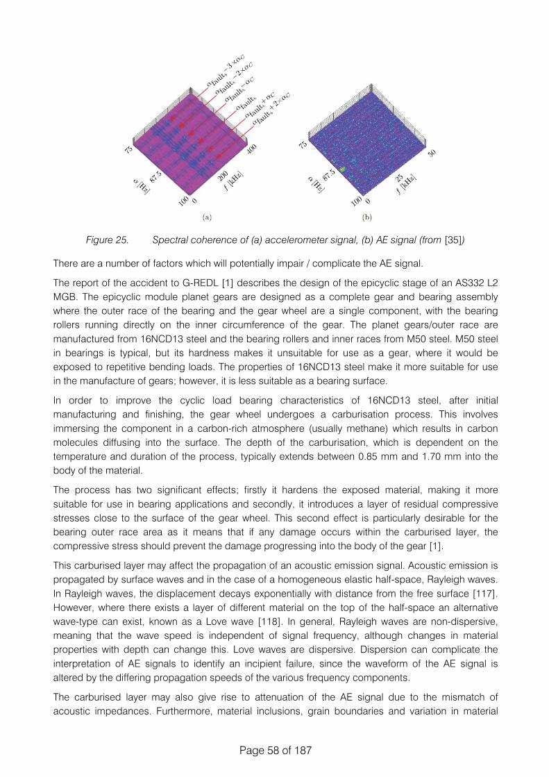
Page 58 of 187
Figure 25. Spectral coherence of (a) accelerometer signal, (b) AE signal (from [35])
There are a number of factors which will potentially impair / complicate the AE signal.
The report of the accident to G-REDL [1] describes the design of the epicyclic stage of an AS332 L2 MGB. The epicyclic module planet gears are designed as a complete gear and bearing assembly where the outer race of the bearing and the gear wheel are a single component, with the bearing rollers running directly on the inner circumference of the gear. The planet gears/outer race are manufactured from 16NCD13 steel and the bearing rollers and inner races from M50 steel. M50 steel in bearings is typical, but its hardness makes it unsuitable for use as a gear, where it would be exposed to repetitive bending loads. The properties of 16NCD13 steel make it more suitable for use in the manufacture of gears; however, it is less suitable as a bearing surface.
In order to improve the cyclic load bearing characteristics of 16NCD13 steel, after initial manufacturing and finishing, the gear wheel undergoes a carburisation process. This involves immersing the component in a carbon-rich atmosphere (usually methane) which results in carbon molecules diffusing into the surface. The depth of the carburisation, which is dependent on the temperature and duration of the process, typically extends between 0.85 mm and 1.70 mm into the body of the material.
The process has two significant effects; firstly it hardens the exposed material, making it more suitable for use in bearing applications and secondly, it introduces a layer of residual compressive stresses close to the surface of the gear wheel. This second effect is particularly desirable for the bearing outer race area as it means that if any damage occurs within the carburised layer, the compressive stress should prevent the damage progressing into the body of the gear [1].
This carburised layer may affect the propagation of an acoustic emission signal. Acoustic emission is propagated by surface waves and in the case of a homogeneous elastic half-space, Rayleigh waves. In Rayleigh waves, the displacement decays exponentially with distance from the free surface [117]. However, where there exists a layer of different material on the top of the half-space an alternative wave-type can exist, known as a Love wave [118]. In general, Rayleigh waves are non-dispersive, meaning that the wave speed is independent of signal frequency, although changes in material properties with depth can change this. Love waves are dispersive. Dispersion can complicate the interpretation of AE signals to identify an incipient failure, since the waveform of the AE signal is altered by the differing propagation speeds of the various frequency components.
The carburised layer may also give rise to attenuation of the AE signal due to the mismatch of acoustic impedances. Furthermore, material inclusions, grain boundaries and variation in material

Page 59 of 187
density which alter the acoustic impedance within the material will affect the wave propagation although these effects should be minimal in a high-grade aeronautical material
In addition to effects due to carburisation, oil lubrication will tend to damp the component surface, thereby attenuating the signal level. This will depend on factors such as oil layer thickness, oil temperature and oil viscosity as highlighted by Tan and Mba [112].
An additional attenuating effect is that of geometric spreading and any associated directionality. Any AE emission produces a finite amount of energy. If this energy is propagated equally in two-dimensions (surface wave) then the finite energy will be equally distributed across the circumference of an expanding circle, giving a reducing energy at any point with an inverse-square relationship. Any directionality, or preferred propagation direction will tend to increase the signal level, but only in the preferred direction of propagation. Finally, curvature (such as in the outer bearing race of a planetary gear) may restrict or focus wave propagation, or alternatively give rise to wave conversion of the AE signal.
Unfortunately, given all of these competing factors, performing a meaningful analysis of likely sensor performance is difficult. It would be possible to establish the propagation behaviour of a Rayleigh wave in a homogenous steel half-space and predict possible decay rates. However, incorporating the damping effects of the oil layer, the layered-media effects of the carburised layer, and the geometric effects of the curved bearing outer race is extremely complex and any estimates are unlikely to be representative.
Clearly, there is the ‘trivial’ solution that a reduced transmission path will yield higher signal levels, and this is borne out by the literature presented earlier; acoustic emission is extremely sensitive to transmission path. However accurately assessing the level of this improvement is not realistic. For this reason, practical testing is proposed to establish the performance of this sensor.
AE Sensors - implementation
Research by Pickwell [119] conducted at Cranfield University showed that the development of a functioning MEMS AE sensor (approximately 20 µm thick) was possible and comparison with commercial AE sensors provided some confidence in the performance of the sensor. However, this research work focused more on the design and physical production of these sensors rather than the detail of their performance.
Figure 26. A thick film PZT Acoustic Emissions device (left) alongside a commercially available PICO sensor (right).

Page 60 of 187
The PAC PICO sensor, is a miniature (5mm diameter, 4mm height) acoustic emission sensor. It has an operational temperature range of -65˚C to +177˚C and weighs less than 1 gram. As with the MEMS sensors, it requires signal conditioning / preamplification and acquisition hardware.
Figure 27. PICO miniature acoustic emission sensor (from www.pacndt.com)
Figure 28. Comparison of thick film AE sensor with commercial sensor from [119]
As with the vibration sensors described above, the thick film AE sensors will require additional circuitry to condition the signal and transmit the signal wirelessly and as such will require power to function. It should be feasible to obtain this through power harvesting, although space limitations may prevent the use of this approach directly on the planetary gear. However, it should be possible to implement power harvesting and house the required circuitry within the planet carrier and mount an AE sensor on the planet carrier shaft.
AE sensors acquire data at high sampling frequencies, typically 1 – 5 MHz and this can place heavy constraints on the on-board data storage. This would also be a key consideration if wireless AE sensors were used. This will be discussed later in this report.
Acoustic Sensors - general
As already mentioned, there has been some successful work aimed at detecting faults using the noise generated by the gearbox. However, unlike traditional HUMS vibration monitoring there has been little focus on gearbox noise for helicopter gearbox prognostics.
Whilst the use of microphones is simple, the signal processing that would be required to give health indications can be less than trivial. However, because the transmission path for acoustics is so much more ‘open’ than in the case of vibration there is the potential for more information to reach the sensor.
!
CHAPTER 5. EMBEDDED MEMS AE DEVICES 107
In these tests the rise time between 10% and 90% was 3.66µs longer in the thick
film device than the PICO sensor, the standard deviation in the rise time varia-
tion was 0.33µs. Table 5.1 indicates that the maximum amplitude and the signal
energy of the the thick film device were approximately 18.5 and 12 times lower
than that of the PICO sensor respectively. The data also shows that there was
greater ringing in the thick film device signal, measured as the duration the AE
signal amplitude was above 10% of maximum amplitude, than the PICO sensor.
The time and frequency domain plots of representative AE signals detected by
both the thick film and PICO sensors are shown in figure 5.3. In this figure the
initial 500µs of the time domain is shown on the left and the frequency spectrum
of the time domain signal, calculated by use of FFT, is shown on the right. The
thick film signal is shown here above the signal detected by the PICO sensor.
Figure 5.3: Plot showing the initial 500µs of the time domain (left) and frequencydomain (right) signals detected by the thick film device (top) and the PICOcommercial sensor (bottom). The signal to noise ratios of the thick film andcommercial devices were 63.1 and 120.6 respectively.
Spectrograms of the initial 20µs of the time domain signals from the thick film
and PICO sensor were calculated using AGU Vallen Wavelet software (release
A2009.1027) from Vallen Systeme GmBH. The AGU Vallen Wavelet software op-
erates on a Gabor transform with a transform window of 20µs. Vallen Systeme
GmBH Vallen Dispersion software (release A2009.1027) was used to calculate
dispersion curves for Lamb waves in the Kovar plate, based on the dimensions
and physical properties of the plate material. These plots can be seen in figure

Page 61 of 187
Acoustic Sensors - performance
Baydar and Ball [120] successfully tested acoustic diagnosis of gear damage against vibration noting that “it has been shown that acoustic condition monitoring can effectively be used for fault detection in gearbox operation”. However, they also noted that “the position of the microphone and its proximity to other components (acoustic sources) play a critical role in the successful application of acoustic condition monitoring”. The acoustic signal provided information to detect the failures from 30% tooth removal and from 2mm tooth crack. They also noted that the vibration signal outperformed the acoustic signal, allowing detection at 20% tooth removal and 1mm tooth crack.
Acoustic sensors - implementation
MEMS passive acoustics sensors would require typical power of around 150 mW. However, since only ‘acoustic access’ is required to the gearbox a more simple approach would be to use conventional microphones placed in an opening in the gearbox casing. This allows the data acquisition, power and signal processing to be retained outside the casing. Acoustically transparent screening would be used, or fluid-tolerant microphones.
6.6. Wireless transmission technology
There is a range of wireless transmission standards which could be employed including ‘WiFi’ (IEEE 802.11), ‘Bluetooth’ (IEEE 802.15) and ‘ZigBee’ (IEEE 802.15). Table 10 summarises some of the key features of each of these technologies.
For this application, ZigBee represents the most appropriate protocol because of its low power consumption, low cost and short join time. ZigBee nodes can go from sleep to active mode in 30 ms or less, the latency can be low and devices can be responsive, particularly compared to Bluetooth wake-up delays, which are typically around three seconds. However, ZigBee does have a limited network speed which will not handle sampling rates in the order of megaHertz (ZigBee can support around 8 kHz sampling rates at 32 bit resolution or 32 kHz at 8 bit resolution). Therefore, in order to support typical acoustic emission sampling rates it would be necessary to pre-process or cache the data and transmit at a controlled rate.
Bluetooth can offer higher transmission rates and hence support higher sampling rates (32 kHz at 32 bit resolution or 128 kHz at 8 bit resolution) although this will still not permit real-time megaHertz sampling rates. A 2 MHz sampling rate at 32 bit resolution would require sustained 64 Mbps which would be challenging for even the 802.11n WiFi standards. Therefore, any of these wireless protocols will require pre-processing or caching to work at high acoustic emission sampling rates. However, typical vibration sampling rates can be easily supported.
Arrays of wireless acoustic emission sensors have been successfully deployed using Zigbee for structural monitoring of bridges and large structures [121], [122]. However, all of these applications had significant flexibility on size of the installation and also the power available.
Using RF interrogation, transmission distances of metres are possible, with centimetres being easier, requiring reduced power levels. In [108], a bench test setup for reliable wireless strain measurement at a distance up to 5 cm was demonstrated. There may be a shielding effect from the planet carrier or from gears but it should be possible to position transmitters and pickups to alleviate any difficulties.
At present, it is not feasible to combine MEMS sensors with pre-amplifiers, power harvesting and wireless transmission into a single MEMS device, although clearly this is a desirable goal. Pickwell [119] notes that “Screen printing is one possible manufacturing technique which may be appropriate

Page 62 of 187
and this may be combined with the development of PZT/polymer materials enabling low processing temperatures which allows the integration of MEMS devices with a wider range of structural elements.” However, this is not a currently available solution.
WiFi Bluetooth ZigBee IEEE 802.11 IEEE 802.15 IEEE 802.15
Max range 50-100 m
30 m indoors 100 m outdoors
10-100 m 10-100 m
Frequency 2.4 & 2.5 GHz 2.4 GHz 868 MHz Europe 900-928 MHz US
2.4 GHz World Power
consumption High Medium Low
Application Video, email, web Cable replacement &
Mobility
Aimed at grand scale automation & remote
control Max network
speed >11 Mbits/sec 700 kbit -1 Mbit/sec 20-250 kbit/sec
Network join time 3 seconds 30 milliseconds Network size 30 7 Unlimited
Cost Medium Low Low Cost
(terminal units) High Low Low
Table 10. Candidate wireless communication protocols
6.7. Power harvest ing
One typical form of power harvesting uses vibration / displacement of piezoelectric material to generate a charge or voltage which can then be exploited. For example, 13 mW typical energy output has been produced by a patch attached to a cantilever, at 1G acceleration, 10 Hz and 800 ppm strain. However, in the epicyclic stage the opportunities to exploit this technique are limited. One possibility is to place a macrofibre composite patch between the inner bearing race and planet carrier shaft. However, the displacements induced at this point may not be suitable for harvesting and the life of PZT components may be limited in this location.
An alternative means of power harvesting may be to employ Faraday’s law to induce currents in a conductor moving in a magnetic field. By mounting magnets on a planetary gear and a conductor on the planet carrier, power harvesting should be possible dependent on the magnetic field, rotation speed, configuration etc. Power harvesting in the range of tens to hundreds of mW should be achievable. Clearly, gearbox material considerations will be crucial in this situation.
6.8. Down-select ion process and conclusions
The initial sort process, the consideration of practical restrictions and the deeper analysis of sensor performance has decimated the list of solutions proposed by the initial search. The restrictions on size, weight and environment provided significant restrictions that were not easily avoided.
Despite these restrictions, a number of solutions have been brought forward which should offer a significant improvement in defect signal level whilst also satisfying the strict requirements imposed for operation within the gearbox casing.
!
Page 63 of 187
The potential sensing solutions that have come from this analysis are:
• Passive microscale temperature sensors with RF interrogation
• Passive microscale strain sensors with RF interrogation
• Active vibration microscale sensors with power harvesting and wireless data transfer
• Active vibration/strain patch sensor with power harvesting and wireless data transfer
• Active AE microscale sensors with power harvesting and wireless data transfer
• Acoustic monitoring from access points in the gearbox casing
The first two solutions are suitable for being attached to the planetary gear directly since they are microscale, require no additional circuitry and require no power harvesting. Of the two, strain is more likely to give useful information since, by its nature, temperature response will be slow and be disposed to diffusion of energy. That said, temperature measurement may provide useful supporting information in the context of gearbox operation particularly close to the bearings; if strain measurements suggest the growth of a defect and that gear also has a higher temperature then there will be greater confidence in the diagnosis.
The second three solutions are more ‘traditional’ sensing mechanisms for machine prognostics, with vibration being the HUMS status quo, and acoustic emission being well-established in the field. However, the nature of the sensors is such that passive RF interrogation approach will not work for these sensors, instead requiring power and circuitry to offload usable data. Because of these restrictions, these sensing solutions are considered to be only appropriate for attaching to the planetary carrier. Power harvesting should be possible and there should be space in which to store the associated circuitry. However, the risk to the gearbox posed by having circuitry installed within it cannot be ignored.
By having a number of constant monitoring positions available on the planetary gear, it might be possible to enhance the signal processing being carried out. By calculating whether signals are arising, say, when planetary teeth interact or when bearings pass over a particular point it may be possible to infer more accurately the location of the damage. Also, having some sensors positioned on the planetary gear, and some positioned on the planetary gear carrier will further enhance the opportunities for differential signal processing.
Finally, acoustic monitoring is low risk with regard to sensors since ‘standard’ microphones can be positioned in or around the gearbox casing to collect data. The greater risk with this approach is whether incipient damage can be detected using acoustic signals. Gross damage and impending failures are certainly available, but whether this would offer any advantage over real-time vibration monitoring or similar is unclear.
6.9. Conclusions
In order to select between the different detection mechanisms, laboratory-scale testing was conducted on a representative configuration, and this is the subject of the next Chapter.

Page 64 of 187
7. Laboratory-scale test ing
7.1. Introduction
In order to understand, test and validate the performance of acoustic emission as a sensing technique, a range of laboratory-scale tests were performed. By seeding faults in a representative setup it was possible to evaluate, in a controlled condition, the detection potential of Acoustic Emission (AE) in comparison with more established vibration techniques, for a range of faults.
7.2. Experimental setup
A pre-existing gear rig was used for the measurements. The gear rig was originally designed as a ‘back-to-back’ (2 gear) setup as shown in Figure 29 below. The input motor and input shaft are mounted on a moving plate allowing motion of the input shaft relative to the output shaft.
Figure 29. Existing gear rig with two shaft setup
However, in order to provide the most representative test conditions with which to study a helicopter gearbox, the rig was significantly modified. The detail below describes the rig as tested, after modification.
The rig uses three gears, an input gear, an idler gear and an output gear, to approximate a single planet of an epicyclic setup as shown in Figure 30 below.
Figure 30. Schematic of planetary representation by 3 gear train

Page 65 of 187
Input drive is provided by a Brooks Compton motor, running at a fixed speed of 1500 rpm. The motor output uses a flexible spider coupling to drive an input shaft, which is supported by two SKF SYJ507 bearings, shown in Figure 31 below.
The end of the input shaft passes into a steel-walled oil sump, with a clear perspex lid with gasket. On the end of the input shaft, a 17 tooth, module 4, 68 mm pitch diameter gear is located by a parallel key in the shaft and a corresponding notch in the gear, and is retained by a nut and secondary locknut. The gear is 25 mm thick and is made of case-hardened steel. This setup was intended to economically best replicate a single MGB planet gear in a research environment.
Figure 31. Motor output, coupling and gearbox input shaft
Mounted between the pre-existing shafts is a new idler shaft, mounted on a support, which is in turn bolted to the moving plate of the gear rig. The non-rotating idler shaft supports an 18 tooth, module 4, 72 mm pitch diameter idler gear which is driven by the input shaft and gear. Rotation of the gear relative to the idler shaft is facilitated by a pair of taper-roller bearings, type SKF 32005 X/Q, which allow some pre-load to be applied. The bearing outer races are a press-fit into the gear and they are retained by a threaded ring with a locking bolt which tightens against the shaft. The bearings were lubricated using multi-purpose lithium grease with a working temperature range of -15°C to 135°C. The shaft caps were tightened to 15 Nm torque.
Gear Input gear Id ler gear Output gear
Number of teeth 17 18 19
Module (mm) 4
Pitch diameter (mm) 68 72 76
Helix angle (°) 90
Facewidth (mm) 25
Material EN36c steel, ground case harden to give a case depth core tensile strength of 1080 Nmm2
Oil Ester synthetic, Kinematic viscosity@ 40o c 11000 mm2/s !

Page 66 of 187
The chosen gear teeth give the asynchronous rotation that is typical of epicyclic configurations.
Figure 32 shows a cross-section of the idler shaft, bearings, idler gear and locking ring, and Figure 33 shows the assembled shaft, bearings, gear and support. Figure 34 shows the input, idler and output shafts in the sump, with the gears removed.
Figure 32. Section through shaft, bearings, idler gear and locking ring
Figure 33. Idler shaft support and idler gear

Page 67 of 187
Figure 34. Three parallel shafts (gears removed)
The idler gear meshes with a 19 tooth, module 4, 76 mm pitch diameter output gear, which is keyed to the output shaft in the same way as the input gear is to the input shaft. The output shaft is connected to a liquid-cooled Shenk dynamometer supplying a selectable torque braking torque up to approximately 14 kW.
The system was lubricated using Synthetic AeroShell Turbine Oil 555, force fed by a Watson-Marlow 323S peristaltic pump with a 313DW pumphead, rotating at 300 rpm feeding 8 mm bore pipe to give a flow rate of approximately 1500 ml/min. This feed was divided between two feed pipes, one feeding from above the mesh point between the input and idler gear and one feeding from below the mesh point between idler gear and the output gear (due to the opposite rotation direction).
Data acquisition
4 uniaxial accelerometers, Dytran 3055B2 (100 mV/g), were positioned on the rig, one on the input shaft bearing closest to the gear, acting in the x-direction, and three in orthogonal directions on the output shaft bearing closest to the gear. A miniature triaxial accelerometer, PCB 356A03 (10 mV/g), was mounted on the idler shaft next to the AE sensor, a PAC Pico connected to a PAC 2/4/6 pre-amplifier, with gain set at 40 dB, as shown in Figure 35.
Figure 35. AE sensor and triaxial accelerometer mounted on idler shaft
Page 68 of 187
A microphone was placed in a mount on the test bed, approximately 15cm from the corner of the oil sump. A 60-segment encoder was acquired from the dynamometer on the output shaft as a rotational measure.
The accelerometers, microphone and rotary encoder were captured using a NI cDAQ-9172 chassis, controlled over USB using MATLAB, at a sample rate of 51.2 kHz. The accelerometer and microphone were acquired using a NI 9234 module, and the rotary encoder using a NI 9215 module. At each load setting, 60 seconds of data was captured.
Data from the AE sensor were captured using a PAC PCI-2 data acquisition card, sampling at 5 MHz, with high-pass filtering at 100 kHz and low-pass filtering at 2MHz. At each load setting, approximately 5 seconds of waveform was streamed in WFS format using AEWin software.
7.3. Transmission test
In order to give confidence in the potential of AE to detect incipient failures in bearings, a transmission test was performed. The source for this test was provided by breaking a pencil lead on the location of interest and monitoring the response (the Hsu-Nielsen test).
The results, which are given in Annexe 5 show that an identifiable AE signal can be transmitted from the teeth of the gear to the end of the shaft, and also from all points between to the end of the shaft. This test shows that there is a basis for expecting an AE signal to be transferred. If this signal were not evident, there would be little to support pursuing AE as a detection mechanism.
7.4. Load
Load is a key factor both in the strength of any defect signal and in the background noise generated. Therefore, a range of dynamometer load settings were studied, ranging from no load (0%) up to full load of 10 kW (100%), in steps of 1 kW. Measurements were then taken reducing the load from 100% back down to 0%. These second measurements were made in order to capture any hysteresis, temperature or time-dependent effects that might affect the tests. The dynamometer is not always able to supply exactly zero load, with a setting of zero sometimes giving a load up to the order of 0.3 kW. Equally, there was fluctuation in the load applied by the dynamometer, of the order of ±2%. The output speed varied with applied load from 1340 rpm at zero load, down to approximately 1322 rpm at 10 kW load.
7.5. Alignment
Alignment of both gears and shafts is key to producing quiet running gears. In gearboxes this is normally achieved by either tight manufacturing tolerances or by allowing the gears to self-align. The epicyclic stages of the Puma gearbox uses a combination of these approaches.
In order to allow flexibility in its use, the gear rig has been designed with variable gear and shaft alignments. However, this means that care needs to be taken when aligning the rig. In the past, with a two-shaft configuration this has been achieved using a micrometer measurement from an arbitrary reference plane. However, in the three-shaft configuration, this is considerably more complex.
Therefore, in an attempt to facilitate and improve the alignment, a new procedure was developed using a measurement arm. This is a measurement system using rotary encoders and precise length shafts to calculate the position of the probe at the end of the articulated arm. The model used in this case, an 8 ft FARO Quantum, has a single measurement accuracy of 20 microns (0.020 mm).

Page 69 of 187
Measurements were taken from each section of shaft of interest and in each case a cylinder was fitted to the measurements. This allows a best fit of multiple measurements to be gained, whilst taking advantage of the knowledge of the shape of the part, rather than simply averaging measurements of a single point.
Once fitted, the axis of the cylinder can be used to check the angular alignment of the shaft relative to another shaft. In this case the output shaft was used as the reference since it is fixed, whereas the input shaft and idler shaft are adjustable.
Figure 36. Rig alignment measurements
7.6. Bearing damage
The pre-assembled construction of the bearing meant that damage to the inner race was not possible. However, this was not considered to be a significant restriction since signal transmission from the inner race is likely to be easier than from the outer race.
The testing used seeded defects of known size and location to establish the detectability of such damage, rather than using long run times to try and develop or propagate damage.
The damage was created using electric-discharge machining (EDM) also known as spark erosion. The electrical discharge cutting, and material removal process involves no contact and no loading on the part machined. Accuracies of +/- 0.005mm can be achieved. This process provides good repeatability allowing multiple bearings to be damaged in the same way.
Three levels of damage were specified:
Gross - a slot running axially along the bearing race, 2 mm wide, 1 mm deep;
Marginal – a spot, 2 mm diameter, 0.5 mm deep; and
Slight – a spot, 1 mm diameter, 0.25 mm deep.

Page 70 of 187
Figure 37. 5 damage conditions for bearing
The gross damage was applied to the outer race of the bearing and the marginal and slight damage were applied to either the outer race or a single roller, creating 5 different damage conditions, with no damage representing a sixth condition. The damage conditions are shown in Figure 37.
The damaged bearing was placed in the side of the gear closest to the sensor end of the shaft.
Table 11 describes the testing programme and Table 12 the specific frequencies associated with the different rotational speeds and damage types.
!

Page 71 of 187
Test Number Outer Race Rol ler Notes 0 - - Background noise 1 - - Good condition 2 - - Check repeatibility 3 Slight - 4 - Slight 5 Marginal - 6 - Marginal 7 Gross -
Table 11. Tested conditions
Component Frequency (Hz)
Motor Shaft 25
Intermediate shaft 23.6
Dynamometer shaft 22.4
Gear Mesh Frequency (GMF) 425
Outer Race Defect (ORD) frequency 192
Table 12. Spectrum frequency components
7.7. In i t ia l results
Only those results relevant to the detection of outer race damage will be presented.
Figure 38. Kurtosis of AE signals

Page 72 of 187
Figure 39. RMS of AE signals
The rms and kurtosis results show that the gross damage can be easily distinguished. However, all of the other results give similar levels, with no apparent pattern to the slight differences.
In hindsight, the use of small sunken damage with a roller bearing (rather than a ball bearing) limited the level of signal that was generated. This is because a ball would drop into the defect whereas the roller is better able to ride over the defect with support from both sides.
For these reasons, an alternative analysis approach was explored.
7.8. Advanced signal processing
Several authors have proposed numerous diagnostic approaches for planetary gearboxes, with vibration analysis the most commonly employed monitoring technology [123]-[128]. However, fault detection of bearings within the planetary gearbox is one of the most challenging diagnostic scenarios, as the resulting vibration signatures are influenced by the variable transmission paths from the bearing to the receiving externally-mounted sensor. This leads to strong background noise which can mask the vibration signature of interest. This task is compounded by the fact that the gear mesh frequencies typically dominate the resultant vibration signal [124], [127], [129].
Early attempts utilized time domain averaging to separate the gear components from the measured vibration signal in order to improve the signal-to-noise ratio (SNR). This involves combining a delayed version of the measured vibration signal with the original signal thereby reinforcing certain frequency components, whilst eliminating others. However, the SNR enhancement with this technique is not always sufficient to aid detection of bearing faults and hence this technique has not proved successful in identifying bearing defects within planetary gearboxes [124]. Time Synchronous Averaging (TSA) has also been applied to separate the bearing vibration components from the measured gearbox signature [127], [130]-[133]. This minimises the influence of speed variation by re-sampling the signal in the angular domain [127]. The process of re-sampling the signal requires a
Page 73 of 187
tachometer or phase marker and is not commonly applied for the sole purpose of separating the bearing vibration signature [132].
More recently, signal separation techniques have been applied in the diagnosis of bearing faults within gearboxes. The separation is based on decomposing the signal into deterministic and random components. The deterministic part represents the gear component and the random part represents the bearing component of the measured signal. The bearing contribution to the signal is expected to be random due to slip effects [132], [134]-[136]. A number of methods for signal separation are available, each having relative advantages and disadvantages [132], [137]-[139]. Techniques such as Linear Prediction (LP) have been employed for separation, allowing the separation of the deterministic (or predictable) part of a signal from the random background noise using the information provided by past observations [140], [141]. The results of such techniques depend on the number of past observations considered. Smaller values of past observation produce a poor prediction, giving a result of negligible improvement in the signal-to-noise ratio, while very high values compromise computation time, over-constrain the prediction and tend to reduce even the main components of the signal (both deterministic and non-deterministic parts) [142], [143]. Interestingly LP is applied only to stationary vibration signatures.
To overcome the problem of separation of non-stationary vibrations, adaptive filters were proposed. This concept is based on the Wold Theorem, in which the signal can be decomposed into deterministic and non-deterministic parts. It has been applied to signal processing in telecommunication [143] and ECG signal processing [144]. The separation is based on the fact that the deterministic part has a longer correlation than the random part and therefore the autocorrelation is used to distinguish the deterministic part from the random part. However, a reference signal is required to perform the separation. The application of this theory in condition monitoring was established by Chaturvedi et al. [145] where the Adaptive Noise Cancellation (ANC) algorithm was applied to separate bearing vibrations corrupted by engine noise, with the bearing vibration signature used as a reference signal for the separation process. However, for practical diagnostics, the reference signal is not always readily available. As an alternative, a delayed version of the signal has been proposed as a reference signal and this method is known as self-adaptive noise cancellation (SANC) [136] which is based on delaying the signal until the noise correlation is diminished and only the deterministic part is correlated [135].
Many recursive algorithms have been developed specifically for adaptive filters [146], [147]. Each algorithm offers its own features and therefore the algorithm to be employed should be selected carefully depending on the signal under consideration. Selection of the appropriate algorithm is determined by many factors, including: convergence, type of signal (stationary or non-stationary) and accuracy [148].
The Spectral Kurtosis technique has been introduced recently for bearing signal separation [149]-[151]. The basic principle of this method is to determine the Kurtosis at different frequency bands in order to identify the energy distribution of the signal and determine where the high impact energy (transient events) are located in the frequency domain. Obviously the results obtained strongly depend on the width of the frequency bands Δf [152]. As noted earlier, in real applications background noise often masks the signal of interest and as a result the traditionally obtained Kurtosis value, in the time domain, is unable to capture the ‘peakiness’ of the fault signal, usually giving low Kurtosis values. Therefore, in applications with strong background noise, the Kurtosis as a global indicator is not useful, although it gives better results when it is applied locally in different frequency bands [151]. The Spectral Kurtosis (SK) was first introduced by Dwyer [153] as a statistical tool which can locate non-Gaussian components in the frequency domain of a signal. This method is able to

Page 74 of 187
indicate the presence of transients in the signal and show their locations in the frequency domain. It has been demonstrated to be effective even in the presence of strong additive noise [151].
In machinery monitoring applications, AE are defined as transient elastic waves produced by the interface of two components or more in relative motion [157], [158]. AE sources include impacting, cyclic fatigue, friction, turbulence, material loss, cavitation, leakage etc. It provides the benefit of early fault detection, in comparison to vibration analysis and oil analysis, due to the high sensitivity to friction offered by AE [159]. Nevertheless, successful applications of AE for health monitoring of a wide range of rotating machinery have been partly limited due to the difficulty in signal processing, interpreting and manipulating the acquired data [160]-[162]. In addition, AE signal processing is challenged by the attenuation of the signal and as such the AE sensor has to be close to its source. However, it is often only practical to place the AE sensor on the non-rotating member of the machine, such as the bearing housing or gearbox casing. Therefore, the AE signal originating from the defective component will suffer severe attenuation and reflections, before reaching the sensor. Challenges and opportunities of applying AE to machine monitoring have been discussed by Sikorska et. al and Mba et. al. [157], [163]. To date, most applications of machine health monitoring with AE have targeted single components such as a pair of meshing gears [164], a particular bearing or valve [165], [166]. This targeted approach to application of AE has, on the whole, demonstrated success. However the ability to monitor components that are secondary to the main component of interest such as a bearing supporting a gear, as is the case with planetary gears in an epicyclical gear box, has not been well-explored. This is the first known publication to explore the ability to identify a fault condition where the AE signature of interest is severely masked by the presence of gear meshing AE noise.
Whilst vibration analysis of gearbox fault diagnosis is well established, the application of AE to this field is still in its early stages [159], [167], [168]. Moreover, there are limited publications on application of AE to bearing fault diagnosis within gearboxes [161]. This section of the report discusses the analysis of vibration and AE data collected from a simplified planetary gear test rig, and compares their effectiveness in diagnosing a bearing defect in the simplified planetary gearbox. The data were collected for various bearing fault conditions and processed using an adaptive filter algorithm to separate the non-deterministic part of the signal and enhance the signal-to-noise ratio for both AE and vibration. The resultant signatures were then further processed using envelope analysis to extract the fault signature.
Gear and bearing diagnosis
The vibration signals associated with bearing defects have been extensively studied and robust detection algorithms are now available as off-the-shelf solutions. Conversely the dynamics associated with bearing diagnostics within gearboxes reduce the capability of traditional techniques. Therefore, it is important to understand the nature of the faulty bearing signal.
For rolling element bearings, a fault will cause shocks which in turn excite higher resonance frequencies which will be amplitude modulated depending on two factors, the transmission path and loading condition [133]. Therefore the vibration signal is typically demodulated to extract the frequency of these impulses. Equations for calculation of bearing faults frequencies have been reported widely in the literature [127], [169], [170]. These equations assume no slip; however, in operation there is some degree of slip and this why the bearing faults frequencies vary by 1% to 2% of the calculated value. It is this slip that facilitates the separation of the gear and bearing vibration components [134], the latter known as the non- deterministic component of the measured vibration.
The deterministic part of the signal is usually related to gear and shaft speeds [128]. Such periodic events are related to kinematic forces induced by the rotating parts such as meshing forces,

Page 75 of 187
misalignment and eccentricity [137]. In some cases the deterministic part of the vibration signal cannot be identified due to speed variation, and therefore it essential to re-sample the signal to the angular domain in order to track speed variation [137], [171]. The deterministic part of the signal can be used for diagnostics of gear and shaft faults.
Similarly, the AE signal can be decomposed into deterministic and non-deterministic parts, which is related to gear and bearing signals. However, processing of AE signals is computationally expensive and only relatively short time series AE signatures can be processed [167]. In application to diagnosis of machine faults, simple AE parameters are typically employed, such as rms, kurtosis, AE counts [157] and demodulation [154]. More recently the use of Spectral Kurtosis and adaptive filters have been employed to facilitate the diagnosis of machine faults with AE [150], [155], [156].
Signal processing and data analysis
Bearing and gear fault identification involves the use of various signal processing algorithms to extract useful diagnostic information from measured vibration or AE signals. Traditionally analysis has been grouped into three classes: time domain, frequency domain and time-frequency domain. The statistical analysis techniques are commonly applied for time domain signal analysis, in which descriptive statistics such as rms, skewness, and kurtosis are used to detect the faults [172], [173]. A fast Fourier transform (FFT) is commonly used to obtain the frequency spectra of the signals. The detection of faults in the frequency domain is based on identification of certain frequencies which are known to be typical symptoms associated with bearing or gear faults. The time-frequency domain methods are composed of the short-time Fourier transform (STFT) [174], Wigner-Ville [172], and wavelet analysis [175], [176]. The use of these detection techniques are feasible for applications where a single component is being monitored however for applications that include several components, such as gearboxes, it is essential to employ separation algorithms.
Adaptive filter
An adaptive filter is used to model the relationship between two signals in an iterative manner; the adaption refers to the method used to iterate the filter coefficient. The adaptive filter solution is not unique; however, the best solution is that which is closest to the desirable response signal [177]. FIR filters are more commonly used as adaptive filters in comparison to IRR filters [178].
The adaptive filter principle is based on Wold theorem, which proposes that the vibration signal can be decomposed into two parts, deterministic P n and random!r!(n). This decomposition process can be represented by the following formula [147]:
x n = P n + r!(n) (1)
The process of separation begins by applying adaptive noise cancellation (ANC). The fundamentals of this method have been detailed, and the general layout of the ANC algorithm is shown in Figure 40 [147], [179].
Figure 40. ANC algorithm [147], [179]

Page 76 of 187
In application of the self-adaptive Least Mean Square (LMS) algorithm, the reference signal in the application of ANC algorithm is replaced by a delayed version of the input signal. In this algorithm, the signal is filtered using a Wiener filter, the coefficients of which should be updated for each step. As a consequence, feedback from the filter output is required to estimate the filter coefficients. This process is repeated for each filter step until the prediction error reaches the minimum value. The adaptive filter is a special case of FIR filter expressed by the following relation:
Y! = ℎ! ∗ x t − i!!!
!!!
(2)
Where, ℎ! is the filter coefficient, x t − i !is corresponding sample of time series signal, and n denotes the number of samples in the input signal.
Equation (2) is similar to linear prediction, however the difference is that the filter coefficient in this case is estimated recursively, based on Least Mean Square Error (LMS).
In order to optimize filter parameters and minimize prediction error, the prediction error ε! should be estimated by [179]:
ε! = d! − !h! ∗ x t − i (3)
where, d! denotes the desirable signal. The filter coefficient should be adjusted to minimize this error function. The error might be random in distribution and as such the expectation of the square error signal is used. This leads to the cost function presented in equation (4), which should be minimised in order to find the optimum filter coefficients. This function is defined by:
E(MSE) = E(12 ! (d! − !h! ∗ x t − i )!) (4)
To optimize the mean square error, the cost function should be minimized.
∂MSE∂h = 0
(5)
The solution of this optimization problem leads to the estimation of the optimum coefficients, this solution known as the Wiener–Hopf filter equation [148]:
h!"# = [R!!]!!!R!" (6)
where, R!! is the autocorrelation function of the input signal, and R!" is cross-correlation between input signal and desirable output. However, in the case of the gearbox signal there is no reference signal; instead a delayed version of the input signal is used. Therefore the Weiner-Hopf equation is written as:
h!"# = [R!!(t − ∆)]!!!R!! (7)
where, R!!(t − ∆) is the autocorrelation of the delayed signal.
!

Page 77 of 187
In practice, the filter size is very large and the Weiner-Hopf equation is difficult to solve. As a result, an approximated adaptive LMS algorithm is proposed [177], such that the coefficients are updated by:
h!!! = h! + 2"!x t ε (8)
In which h!!!!!!!!denotes the updated filter coefficient, and ! denotes the step size of the filter. This latter parameter should be selected carefully; the larger the step size, the faster the convergence, whilst a smaller step size leads to more accurate prediction, but the computation cost is high. The range of step size selection can be expressed as [178]:
0 < ! < 1λ!"#
(9)
Where, λ!"# is the maximum value for eigenvalue for autocorrelation R!!. For a step size greater than !
!!"#, the convergence speed can be reduced.
Envelope analysis
Envelope analysis is applied extensively in vibration analysis for the diagnosis of bearings and gearboxes [125], [129], [133]. As impacts due to the defects excite resonance at higher frequencies, it is possible to identify the frequency of the impacts with the use of envelope analysis. In application, the vibration signal is filtered at high frequencies (structural resonance frequencies) and then the signal is passed through an envelope detector and a low pass filter. The enveloped signal is either presented in the time domain or transformed into the frequency domain in order to identify fault frequency components [65]. In order to detect fault signatures it is important to select filter parameters carefully [149]. In addition, Spectral Kurtosis (SK) has been applied to select such filter parameters [151], [181]. The basic principle of the SK method is to determine the Kurtosis at different frequency bands in order to identify the energy distribution of the signal and to determine where the high impact (transient) energy is located in the frequency domain. Obviously the results obtained strongly depend on the width of the frequency bands Δf [152]. The Kurtogram [140] is a representation of the calculated values of the SK as a function of f and Δf. However, exploration of the entire plane (f, Δf) is a complicated computational task, though Antoni [152] suggested a methodology for the fast computation of the SK.
Observations of vibration analysis
The measured vibration data was processed to estimate the power spectrum of the vibration signal for both damaged and fault-free conditions, see Figure 41. This analysis was performed to assess the ability of FFT spectrum analysis to determine the fault signature. The results show clearly that no distinctive differences can be identified between faulty and fault-free bearing conditions, simply because the defect frequencies were not evident in the spectrum. Therefore the data was further processed using signal separation and Spectral Kurtosis to identify the fault signature as described earlier.
!! !

Page 78 of 187
Figure 41. Power spectrum of original vibration signal for (a) fault-free (b) marginal defect and (c)
gross defect conditions
!
7.00
0.00
1.00
2.00
3.00
4.00
5.00
6.00
Frequency)[Hz]27.5k0 5k 10k 15k 20k 25k
10.0
0.00
1.00
2.00 3.00
4.00
5.00
6.00
7.00 8.00
9.00
Frequency)[Hz]27.5k0 2.5k 5k 7.5k 10k 12.5k 15k 17.5k 20k 22.5k 25k
9.00
0.00
1.00
2.00
3.00
4.00
5.00
6.00
7.00
8.00
Frequency)[Hz]27.5k0 2.5k 5k 7.5k 10k 12.5k 15k 17.5k 20k 22.5k 25k
(b)
(c)
(a)

Page 79 of 187
The Spectral Kurtosis analysis was undertaken on data sets collected from the gear rig for the different fault cases and this yielded the frequency bands and center frequencies which were then used to undertake the envelope analysis. An example kurtogram used to estimate filter characteristics for different defect conditions is shown in Figure 42. The filter frequency bands for each data set case are summarised in Table 13. Spectral plots of enveloped vibration signals following filtration, whose characteristics were determined with the aid of the kurtogram, are shown in Figure 43, Figure 44, and Figure 45.
Case Center frequency
Fc (Hz) Bandwidth
Bw (Hz) Kurtosis
Fault-free condition x-direction 18000 800 0.1
Fault-free condition y-direction 18200 750 0.11
Fault-free condition z-direction 17920 789 0.14
Marginal defect x-direction 19733 1066 0.5
Marginal defect y-direction 18920 1080 0.55
Marginal defect z-direction 20083 917 0.45
Gross defect x-direction 18400 1600 12.8
Gross defect y-direction 18400 1600 12.8
Gross defect z-direction 18400 1600 12.8
Table 13. Filter characteristics estimated based on SK for all three vibration axes
Observation from the spectra of the enveloped signal in the x-direction showed the presence in the spectrum of the large defect. Typical outer race defect frequency (192 Hz), the 2nd harmonic (384 Hz), the 3rd harmonic (576 Hz) and 4th harmonics (768 Hz) were detected for large defect. However the small fault condition was not identified by this analysis. It is apparent that the signal separation still had not completely removed the gear mesh and shaft frequencies, which were detected by envelope analysis.

Page 80 of 187
Figure 42. SK of x-direction of non-deterministic signal for (a) fault-free (b) marginal defect
(c) gross defect
(b)
(c)
(a)

Page 81 of 187
Figure 43. Enveloped Spectra of x-direction non-deterministic signal for (a) fault-free (b) marginal
defect (c) gross size defect conditions
! !
1E#2
0E+0
2E#3
4E#3
6E#3
8E#3
Frequency3(Hz)10005 100 200 300 400 500 600 700 800 900
5E#3
0E+0
1E#3
2E#3
3E#3
4E#3
Frequency2(Hz)10005 100 200 300 400 500 600 700 800 900
1.5E+0
0E+0
2.5E(1
5E(1
7.5E(1
1E+0
1.25E+0
Frequency2(Hz)10005 100 200 300 400 500 600 700 800 900
ORD and its harmonics
(a)
(b)
(c)

Page 82 of 187
Figure 44. Enveloped Spectra of y-direction non-deterministic signal for (a) fault-free (b) marginal defect
(c) gross defect conditions
! !
1.5E%3
0E+0
2.5E%4
5E%4
7.5E%4
1E%3
1.25E%3
Frequency4(Hz)10005 100 200 300 400 500 600 700 800 900
3E#3
0E+0
5E#4
1E#3
1.5E#3
2E#3
2.5E#3
Frequency3(Hz)10005 100 200 300 400 500 600 700 800 900
1.75E+0
0E+0
5E(1
1E+0
1.5E+0
Frequency1(Hz)10005 100 200 300 400 500 600 700 800 900
(b)
GMF and its harmonics
(c)
(a)
ORD and its harmonics

Page 83 of 187
Figure 45. Enveloped Spectra of z-direction non-deterministic signal for (a) fault-free (b) marginal
defect (c) gross defect conditions
!
1.5E%3
0E+0
2.5E%4
5E%4
7.5E%4
1E%3
1.25E%3
Frequency4(Hz)12005 100 200 300 400 500 600 700 800 900 1000 1100
2.5E%3
0E+0
5E%4
1E%3
1.5E%3
2E%3
Frequency3(Hz)10005 100 200 300 400 500 600 700 800 900
1E+0
0E+0
2E&1
4E&1
6E&1
8E&1
Frequency2(Hz)10005 100 200 300 400 500 600 700 800 900
1x GMF
(c)
ORD & its harmonics
(a)
GMF
2 GMF
(b)

Page 84 of 187
Acoustic Emission observations
Figure 46 (a) shows the AE signature prior to, and after signal separation of the deterministic components. Figure 46 (b) clearly exhibited periodic shocks events that were masked by background noise in the original time trace, Figure 46 (a).
Figure 46. Time waveform of AE signal (a) before and (b) after separation
The Spectral Kurtosis was employed to extract the filter characteristics which were utilized for envelope analysis on the non-deterministic component of the AE signature. Associated typical kurtograms of SK analysis are shown in Figure 47. The overall maximum kurtosis for defective bearing conditions was significantly higher compared to the the fault-free condition. The maximum kurtosis increased by 600% for the small outer race defect (18.5) and 3000% for severe defect condition (91.7) in comparison to the fault-free condition (3).
! !
0.6
$0.4$0.2
00.20.4
Time(s)10 0.1 0.2 0.3 0.4 0.5 0.6 0.7 0.8 0.9
4Orig in
0.5
$0.5
$0.25
0
0.25
Time*(s)10 0.1 0.2 0.3 0.4 0.5 0.6 0.7 0.8 0.9
Random*signal*
(a)!
(b)!
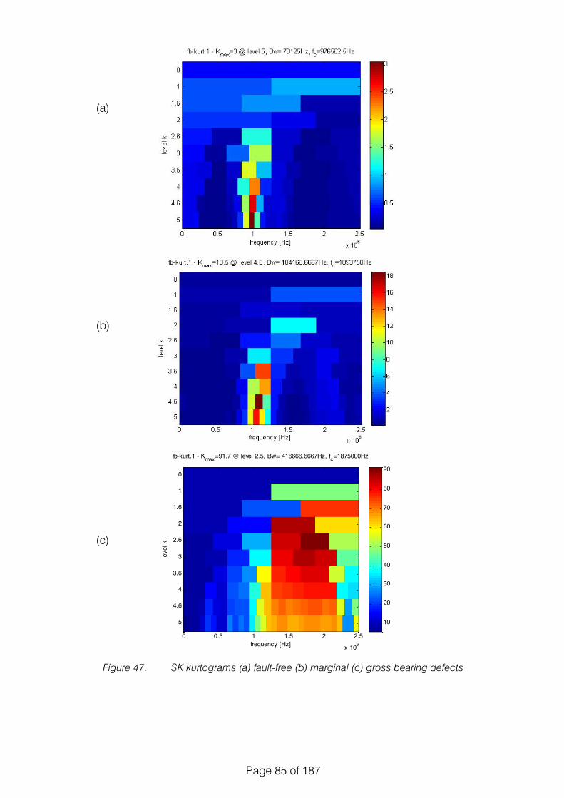
Page 85 of 187
Figure 47. SK kurtograms (a) fault-free (b) marginal (c) gross bearing defects
frequency [Hz]
leve
l k
fb-kurt.1 - Kmax=91.7 @ level 2.5, Bw= 416666.6667Hz, fc=1875000Hz
0 0.5 1 1.5 2 2.5
x 106
0
1
1.6
2
2.6
3
3.6
4
4.6
5 10
20
30
40
50
60
70
80
90
(b)
(c)
(a)

Page 86 of 187
The envelope analysis was undertaken using the central frequency Fc and bandwidth (Bw) estimated by SK analysis, see Table 14. Observations of Figure 48 b) showed the presence of the bearing outer race defect frequency (192 Hz) for the small defect condition. In addition, the outer race defect frequency, and its harmonics, were observed for large defect condition (192 Hz and 384 Hz).
!Case Center frequency
Fc (Hz) Bandwidth
Bw (Hz) Kurtosis
Fault-free condition X direction 976562.5 87125 3.0
Fault-free condition Y direction 976562.5 87125 3.0
Fault-free condition Z direction 976562.5 87125 3.0
Small defect X direction 1093750 104166.667 18.5
Small defect Y direction 1093750 104166.667 18.5
Small Defect Z direction 1093750 104166.667 18.5
Large defect X direction 1875000 416666 91.7
Large defect Y direction 1875000 416666 91.7
Large defect Z direction 1875000 416666 91.7
!Table 14. Filter characteristics estimated based on SK for AE signals
! !

Page 87 of 187
Figure 48. Enveloped spectra of AE signal (a) fault-free (b) small (d) large bearing defects
!
3E#10
0E+ 0
5E#11
1E#10
1.5E#10
2E#10
2.5E#10
Frequency2(Hz)5005 50 100 150 200 250 300 350 400 450
Power2Spectrum2for2Enveloped2for2random2signal2
5E#10
0E+ 0
1E#10
2E#10
3E#10
4E#10
Frequency2(Hz)5005 50 100 150 200 250 300 350 400 450
Power2Spectrum2for2Enveloped2for2random2signal2
8E#7
0E+ 0
1E#7
2E#7
3E#7
4E#7
5E#7
6E#7
7E#7
Frequency5(Hz)5005 50 100 150 200 250 300 350 400 450
Power5Spectrum5for5Enveloped5for5random5signal5
(b)
ORD
(c)
ORD & harmonic
(a)
!
!

Page 88 of 187
Discussion and conclusion
The techniques described above are typically used for applications where strong background noise masks the defect signature of interest within the measured vibration signature. The AE signal is more susceptible to background noise and in this case, the tortuous transmission path from the outer race through the rollers to the inner race, and then the shaft, makes the ability to identify outer race defects even more challenging. Therefore, the use of signal separation to offer further insight into diagnostic information is deemed necessary for application of AE in the diagnosis of planetary gearboxes.
A comparison of the vibration and AE analysis showed both measurements were able to identify the presence of the large bearing defect based on observations in the enveloped spectra. For the small defect condition however, the enveloped spectrum was dominated by the gear mesh frequencies and their harmonics, and as such the bearing defect frequencies were not evident. However AE analysis was able to identify both the small and large defect conditions. Detection of the small bearing defect gives AE an indisputable diagnosis advantage over the vibration analysis.
In summary an investigation employing vibration and AE to identify the presence of a bearing defect in a planetary type arrangement has been undertaken. A series of signal processing techniques were applied to extract the bearing fault signature, which included adaptive filter, Spectral Kurtosis, and envelope analysis. The combination of these techniques demonstrated the ability to identify the presence of the various defect sizes of bearing in comparison to a typical frequency spectrum. From the results presented it was clearly evident that the AE analysis offered much earlier indication of damage than vibration analysis. In addition, the signal processing techniques demonstrated the capability to successfully separate the bearing signal within an AE signal, enhancing the application of AE to gearbox fault diagnosis.
In the context of operational HUMS systems, this technique represents a more advanced and intensive technique than is typical of many HUMS systems. However, the technique was applied to both AE and vibration signals giving a ‘fair’ comparison.
7.9. Sensor select ion
The above analysis suggests that AE offers the greatest opportunity for early detection when compared with vibration and hence this technique was carried forward into full-scale testing. However, the early literature review highlighted a number of sensor options ranging from COTS to experimental sensors from which a candidate sensor had to be selected. The specific sensors considered were: PAC Pico, PAC s9225, PWAS and a custom-made sensor (see Figure 49)
!

Page 89 of 187
Figure 49. AE sensors – PAC s9225 and Pico (top), PWAS (bottom left) and custom fabricated (bottom right)
It was necessary to take a decision balancing the risk of the measurement failing due to sensor problems, and the risk of the sensor being liberated and damaging the gearbox. For the latter consideration, a ‘longer view’ was taken – whilst it may be possible to attach the sensor and limit test runs to ensure the integrity of the gearbox, it was the operational risk of damaging the gearbox that was considered.
The lab-scale tests were performed using the Pico test and this is a useful sensor which provides a reliable signal. However, its size and ‘toughness’ represent a considerable risk to a gearbox if liberated from its fixing.
The custom-made sensor represented very little risk to the gearbox being a few millimetres across and nanometres thick. However, the signal it produces was considered too noisy to guarantee a useful signal and so it was rejected. It is however possible that given the signal levels inside the gearbox that it may be a viable solution in the future.
This left the PWAS sensor and the PAC s9225. In order to select between these two sensors, they were trialled on the gear rig in the same marginal condition which was used to select the AE technique. Both sensors were outperformed by the Pico, which is unsurprising. However, comparing the two sensors, analysis of the signal from the PWAS sensor showed the damage frequencies whereas analysis of the s9225 signal did not display those frequencies.
Therefore, the PWAS sensor was selected for the full-scale tests.
!

Page 90 of 187
7.10. Laboratory-scale wireless transfer
Introduction
This section describes the development of a lab-scale wireless transfer system capable of transmitting an AE signal, consisting of a fixed coil and a rotating coil which moves with the component being investigated, upon which is mounted a sensor.
The sensor-side circuitry is required to be very small and must be self-powered without the use of a battery. To achieve this, the system makes use of Radio Frequency (RF) power-scavenging. The system uses a homodyne receiver with a “modulated backscatter” communications link, to pass the analogue signal across the wireless link.
Choice of frequency and coupling method
RF scavenging to supply dc power wirelessly in tags, has been carried out at the relatively high RF frequencies of 800 MHz and 2.4 GHz. Using an antenna with high gain allows useful power to be transmitted over a long range, in the order of many tens of meters, using a few Watts of RF energy. Note that these systems are termed “far field” and energy transfer is by Transverse ElectroMagnetic (TEM) wave. Huang [182] has demonstrated the transmission of AE signals using an analogue TEM system. A high gain antenna produces a spot beam where the power density is very high, so if that approach were used in this application, the rotating part would need to remain in the spot at all times. Additionally, unless circular polarisation is used on both “transmit” and “receive” antennas, the recovered power would vary at the rotation rate, if the sensor part spins on its axis.
Within an enclosed metal cavity, the use of high frequencies produces a standing wave pattern, where the field falls to zero at regular intervals, typically every half wavelength (about 6 cm at 2.4 GHz). If the receive coil passes through these standing wave nulls, the recovered power will vary, and unwanted modulation will be superimposed on the recovered baseband signal.
Another consideration is the generation of sufficient RF power and licensing since there are controls on use of certain RF powers and frequencies.
For these reasons it was decided to use the 13.56 MHz ISM (industrial, scientific and medical) band, used by other near field, short range devices, such as ISO14443 contactless cards e.g. Mastercard PAYPASS and TFL (Transport for London) Oyster cards.
Operation at 13.56 MHz allows the use of magnetic coupling, where the “antennas” are two tuned loops of wire or pipe. Such coupling is termed near field and relies purely on magnetic coupling, as a conventional transformer for ac mains. The magnetic loop does not produce a TEM “propagating” wave, as in a normal broadcast transmitter. The coupling between two parallel, coaxial coils is consistent as one coil rotates with respect to the other.
Transmission of sensor signal
“Modulated backscatter” is a technique that relies on periodic damping of the resonant circuit of the rotating loop. When magnetically coupled to a receiving loop, the modulation may be detected. In contactless cards, the data is transmitted digitally, in effect a squarewave modulation of an 847 kHz subcarrier. However, in this application, there is a need to transmit a linear analogue signal over a bandwidth extending from 100 kHz to 1 MHz, to preserve the shape of the sensor time domain waveform.
Contactless cards use a “load” modulation scheme, where a damping resistor is switched periodically in parallel with the coil. This is accomplished with a simple on/off FET switch, but the technique is not suitable for a linear system.

Page 91 of 187
As previously discussed, digital transmission of sensor data up to 1 MHz bandwidth at 32 bit resolution would require 64 Mb/s which occupies too much bandwidth for a backscatter technique and would make the sensor circuitry quite complex.
A better analogue modulation scheme is to modulate the resonant frequency of the loop using a varactor diode. Such a diode is a variable capacitor controlled by a “tuning” voltage and has a linear response over a certain voltage range. The electrical change so induced by the varactor diode produces a combination of amplitude and phase modulation of the back-scattered signal.
Detecting the back-scattered signal
The back-scattered signal can be “tapped off” the illuminating coil, so a single coil functions both as transmitter and receiver simultaneously. Using a high quality (low noise) crystal oscillator as both transmit source and receiver reference, enables the use of a so-called “homodyne” (same–frequency) receiver architecture. A portion of the transmitted signal (which is free of modulation) is multiplied with the backscattered signal from the tap at the same carrier frequency, in a coherent demodulator. The output of the demodulator, which responds to both amplitude and phase modulation, is filtered to remove the RF at 13.56 MHz leaving the baseband signal.
Construction of a prototype system
A homodyne receiver operating at 13.56 MHz was constructed, using magnetic coupling loops. The dc power for the sensor conditioning circuit is obtained by rectification of the illuminating field. The signal from the sensor is buffered and modulates the backscatter of the rotating coil. A coherent demodulator in the fixed part of the system recovers the baseband signal which can be fed to data acquisition. Figure 50 and Figure 51 below show the block diagrams for the fixed part (illuminator) and the rotating part (sensor):
Figure 50. Fixed part (illuminator)

Page 92 of 187
Figure 51. Rotating part (sensor)
The associated circuit diagrams are given in Annexe 6.
13.56 MHz source, buffer amp and power amp
A high stability oscillator X1 is used as the transmit source. To ensure the oscillator is not adversely loaded, buffer amplifier Q1 is used to drive the power amplifier Q2, producing approximately 1 Watt of RF output into the illuminator coil.
The buffer amplifier is also required to ensure that the carrier signal has no backscatter modulation present on it, as a pure sine wave carrier is needed as a reference in the coherent demodulator.
Coherent demodulator and filter
The receive input from the illuminator coil tap is fed to the MC1496 demodulator IC, U3. The baseband output from the demodulator is buffered by Q3 and feeds the low pass filter L8, L9, L10 to drive the final amplifier U5. A terminating resistor of value 50Ω sets the output impedance to drive a 50Ω load, such as an ADC card or other acquisition system.
The carrier input to the demodulator is obtained by a connection to the crystal oscillator, through a phase shift network. The carrier phase shifter is necessary to correctly align the carrier phase with the backscattered phase, to obtain the highest baseband output possible from the demodulator IC.
Rotating coil and sensor
The receive loop is tuned by C8 to bring it to resonance just above 13.56 MHz. Diodes D1 and D2 form a rectifier to produce a dc voltage for the opamp U1, smoothed by C1 and C7. The opamp has a gain bandwidth product of 18 MHz and draws 3 mA from a 3.6 V supply.
The sensor output is fed into the high impedance input of the opamp on TP2, which provides a gain of approximately x12. High input impedance is necessary to avoid loading the sensor output. The output feeds a low pass trap L1/L2/C9, to ensure the very high levels of 13.56 MHz do not appear at the amplifier’s output pin, but pass the 1 MHz sensor signal to the varactor diode. A small dc voltage is provided to bias the varactor into its most linear region.
The varactor D3, is loosely coupled to the resonant circuit consisting of the coil and C8 by capacitor C3. With no sensor signal applied to the varactor (just the bias voltage), its capacitance brings the resonance of the circuit to precisely 13.56 MHz

Page 93 of 187
A typical circuit layout for the sensor circuit and coil is shown below in Figure 52 The electronics part could be made much smaller using 0403 size components. The prototype is made on standard FR4 PCB material (fibreglass). However, it could be printed on Mylar film, which is much thinner, more flexible and softer.
Smaller coils may be made – they will need different capacitance values to tune them. Generally, the quality of the recovered signal will fall as the coil becomes smaller. A rule of thumb is that the coil diameter should be √2 x the read range for optimum coupling.
Figure 52. PCB layout for a particular version of sensor circuit and coil, coil is 55mm in diameter
Transmit loop (fixed part)
The circuit for the transmit loop is shown below. C10 and C6 match the coil’s impedance to the 50Ω PA output, depending on the presence of the sensor coil, its distance and orientation. R6 serves two purposes, a) to set the coil’s Q factor and b) to allow a tap-off for the backscattered field. (Q factor is a term indicating the effectiveness of an inductor, defined as energy stored/energy dissipated per cycle).
The Q factor has to be adjusted to allow sufficient Q for the transmission of power, but not too high to limit the system bandwidth, which would cause a drop off in the response at 1 MHz. 0.94Ω (5 x 4.7Ω in parallel) was found to be the optimum value for this size of coil as shown in Figure 53.
Figure 53. Transmit loop circuit (fixed part)
!
L3729nH
R60.94
C6150p
C10
47p
TP4
TP2MM
TP5
TP2MM
TX in
Backscatter out

Page 94 of 187
Set up and test of the system
The electronics unit was powered from a 12 VDC wall block power supply.
Some further setting up was required after installation of the sensor on a metal object. The set up is required as the spacing between the coils changes their mutual coupling, Q and bandwidth and this alters the values needed on the matching network.
The optimum method to ensure the highest bandwidth, is to connect a signal generator in place of the sensor, of about 10 mVpp, sweeping between 100 kHz and 1 MHz. The tuning components on the fixed coil can be adjusted to produce the flattest response, at the expense of signal amplitude.
When installing the sensor board against a metal object, it was necessary to use ARC WAVE-X to avoid detuning the coils.
Figure 54. Transmit loop and matching network (fixed part) prototype and sensor board prototype
Figure 55 shows the frequency behavior of the lab-scale system. As can be seen from the difference trace, the system behaves in a broadly linear way in the 100 kHz to 1 MHz range.
The only known shortcoming of the lab-scale system was the effect of dispersion on the sensor signal which will be displayed in the time domain. Dispersion, sometimes known as non-linear group delay, results when different frequency components in the baseband signal are delayed by different times as they pass through the circuitry. The main cause of dispersion is the sharp phase response of the tuned resonator consisting of the two coils and their mutual coupling. The high Q (and thus dispersive response) is needed to transfer power efficiently, otherwise, much of the RF power would be wasted in the series resistor at the base of the coil.
If the dispersion is consistent, then it can be corrected using software, by delaying different frequencies by appropriate amounts and then reconstructing the time signal

Page 95 of 187
Figure 55. Amplitude linearity of lab-scale coils
! !
0!
10!
20!
30!
40!
50!
60!
70!
80!
90!
100! 200! 300! 400! 500! 600! 700! 800! 900! 1000!
Transmitted!Difference!Source!

Page 96 of 187
8. Full-scale test ing
8.1. Introduction
In order to test and validate the approach outlined by the lab-scale testing, it was necessary to perform full-scale testing of the acoustic emission and wireless transmission concept. Whilst the lab-scale approach tentatively proved the concept, many of the issues surrounding new techniques are only revealed when they are implemented at full-scale.
For this phase of testing, an SA 330 Puma gearbox was acquired from the UK RAF. Although the paperwork for the gearbox was unavailable, the gearbox was believed to be fresh from overhaul, and not to have been installed since overhaul, and its physical appearance appeared to support this. Subsequent investigation with the manufacturer also suggested this to be the case. Figure 56 shows the gearbox supported from a temporary lifting cover.
Figure 56. Purchased SA330 main rotor gearbox
The details of the gearbox are:
Model description: 330 A R G
Assembly No. 32300003
Serial No. ACH9280
Manufacturing date: 10/99
Whilst the SA330 gearbox is an older design, it was the basis of the design of the current EC225 main gearbox, and shares many of the same design features. Most importantly for this project, it has a final two-stage epicyclic reduction utilizing a combined planet gear / outer bearing race design. Figure 57 shows a cross-section drawing.
!

Page 97 of 187
Figure 57. SA330 MGB cross-section from [183]
As part of the HELMGOP II project, Cranfield were developing a test rig capable of driving one input of a Puma gearbox at operational speeds and with some load. However, it could not provide full load and was also under development in parallel with this project and so availability was not guaranteed. As a result, Airbus Helicopters were approached with a request to support the project, around both the technical details of the gearbox and also for access to their test bench facilities, which they agreed to. This was a significant contribution and greatly aided the project.
The Puma gearbox requires specialist tooling and training to be completely stripped and so it was only possible to split the upper planet carrier from the top of the housing a few days before testing was scheduled to start. Because of limitations in opening the gearbox, and also the limited test time available, it was necessary to commit to a testing programme with little opportunity to adjust or develop the sensing approach. This was a significant risk since in a complex, multi-disciplinary project such as this, any single point of failure e.g. wireless transfer or sensor behavior, could render all test data worthless. Testing was conducted in May / June of 2014.
A test programme was devised consisting of tests in three conditions – an undamaged planet bearing; a heavily damaged planet bearing; and a slightly damaged planet bearing (see Section 8.2). The different conditions were achieved by swapping a planet gear between each test. The tests were performed in this order to mitigate the risk of sensor, wireless system and gearbox failure. Each of these three conditions was tested at a range of loads, and with two rotor speeds (see Section 8.6).
On a practical level, working at a remote site complicated the arrangements significantly. For example, the accelerometer glue was not safe for air transport and had to be shipped by road and improvements and modifications to acquisition software could not be tested away from site.
!

Page 98 of 187
8.2. Fault descript ion
In order to test the detection capability of the new system, a fault was seeded on the outer race of two second-stage planet gears, one with ‘major’ damage and with ‘minor’. However, specifying the exact nature of the damage was complex. The aim of the major damage was to produce a defect which was definitely of concern, but which would produce a signal that probably would not be detected by a HUMS system. Similarly, the aim of the minor damage was to produce a defect which represented the start of degradation, and which would produce a signal that definitely would not be detected by a HUMS system. However, knowing the damage conditions which correspond to these levels is extremely difficult. In addition, the available mechanisms for producing the damage had to be considered. The advice of the manufacturer and EASA was sought, and the following rationale was produced.
At early stages, due to the “snow ball effect” the fault propagates in a conical way, see Figure 58a. Once the fault area is large enough, the shape of the fault is more rounded as shown in Figure 58b.
Figure 58. a) Early and b) late stage bearing race damage from [184]
This damage geometry was approximated in this study as a rectangle with fixed depth and width. The fault-to-rolling element length ratio dictates whether the fault is extended (major) or not (minor). Experience from the manufacturer, supported by reference [185] suggests that the surface of the fault should be irregular. The defect length for the major damage is 30 mm (which is around 41° of the circumference) and 10 mm for the minor damage and around 0.3 mm deep. Table 15 below, taken from [1] shows spalling events which had been noted by the manufacturer.
ETG 375 /14 21/05/2014
1 /
AIRBUS HELICOPTERS RESTRICTED
From: Victor Girondin Date:20/05/2014
To :
CU : Greaves, Matthew [email protected] EASA : [email protected] AH : Areny, Pascal [email protected]; Mailhe, Magali [email protected] ; ;; Pillot, Remi (Ste
Assystem) [email protected] ; Sorrentini, Jacques (Ste Manpower) [email protected] Copy : Subject : Bearing Fault Seeding Justification for DER3835 “Cranfield”
The test specification described in [7] is part of a research program, funded by EASA and carried out by Cranfield University (CU), to improve detection of second stage planetary gear bearing defects. The aim of the test program is to measure whether it is possible to detect planetary gear bearing degradation using a sensor mounted inside the gearbox. For this purpose, it has been decided to seed a fault on the outer race of one of the second stage planet. The purpose of this note is to justify the geometry of the seeded fault. The MGB is an SA330 MGB provided by Cranfield University.
The fault specification is described in the documents [6]. The following paragraph explains the chosen pattern and proposes references to back it. At early stages, due to the “snow ball effect” the fault propagates in a conical way as shown on the left figure below [2]. Once the fault area is large enough, the shape of the fault is more rounded as shown on the right figure below [2].
Airbus Helicopters has proposed to model this geometry as a rectangle with fixed depth and width. The fault-to-rolling element length ratio tells is the fault is extended or not. According to AH expertise and [3], the faulty surface shall be irregular. Airbus Helicopters choice is not exotic as the following examples prove it:
Natural fault: [1] “Flaking Surface of the raceway and rolling elements peels away in flakes. Conspicuous hills and valleys form soon afterward”

Page 99 of 187
Table 15. Manufacturer reported spalling events from [1]
For comparison, earlier work has noted the following damage conditions:
Natural fault: “Flaking Surface of the raceway and rolling elements peels away in flakes. Conspicuous hills and valleys form soon afterward” [186].
Figure 59. Natural fault from [186]
Natural fault: “Development of fatigue damage on the inner ring raceway of an angular contact ball bearing. The periodic intervals between inspections from damage begin on, are given in percentage of the nominal life” [184].
73
Air Accident Report: 2/2011 G-REDL EW/C2009/04/01
© Crown Copyright 2011 Section 1 - Factual Information
1.18.3 Events with G-REDN
In July 2010, magnetic particles were found on all three magnetic chip detectors of an AS332 L2 MGB (G-REDN), during a routine 25 hour inspection. The main module chip detector light in the cockpit had not operated and there were no chip detection warnings recorded by HUMS. No particles had been found on the epicyclic chip detector during its last routine inspection, 10 hours prior to the discovery of the particles. After completion of the required maintenance actions, the number of particles collected exceeded the prescribed limitations and the gearbox was removed for investigation. When the gearbox was disassembled, the particles were found to have been generated as a result of a failure within the left accessory gearbox drive module bearings.
In March 2011, several small magnetic particles were found on the main module magnetic chip detector of the MGB installed on G-REDN in July 2010. Analysis of these particles by the manufacturer confirmed that one of these was 16NCD13 steel, but of insufficient size to bridge the contacts of the chip detector and illuminate the main module chip detector light in the cockpit. After discussions between the operator and the manufacturer, the helicopter was placed on ‘close monitoring’ for 25 flying hours.
At the end of this period no additional particles had been found and the ‘close monitoring’ procedure was discontinued. During a routine inspection on 27 April 2011, 87 flying hours after the discovery of the first particle, another three particles were found attached to the main module chip detector. One
Table 2Manufacturer reported spalling events
ETG 375 /14 21/05/2014
AIRBUS HELICOPTERS RESTRICTED
Natural fault: [2] “Development of fatigue damage on the inner ring raceway of an angular contact ball bearing. The periodic intervals between inspections from damage begin on, are given in percentage of the nominal life”
Seeded fault: [3] “An extended fault has been inserted to the inner race of a Koyo 1205 bearing by grinding one eighth of the circumference (12 mm)”

Page 100 of 187
Figure 60. Natural fault from [184]
Seeded fault: “An extended fault has been inserted to the inner race of a Koyo 1205 bearing by grinding one eighth of the circumference (12 mm)” [185].
Figure 61. Simulated inner race damage from [185]
Natural fault: The following pictures present a degraded planet bearing rolling element from a Sea King helicopter [187].
ETG 375 /14 21/05/2014
AIRBUS HELICOPTERS RESTRICTED
Natural fault: [2] “Development of fatigue damage on the inner ring raceway of an angular contact ball bearing. The periodic intervals between inspections from damage begin on, are given in percentage of the nominal life”
Seeded fault: [3] “An extended fault has been inserted to the inner race of a Koyo 1205 bearing by grinding one eighth of the circumference (12 mm)”

Page 101 of 187
Figure 62. Sea King planet bearing damage from [187]
Natural fault: “Vibration acceleration signals were obtained from an overload test of a Bell 206 Helicopter Main Rotor Gearbox in order to complete a blind bearing fault analysis where no knowledge of the fault was made available prior to the analysis.” [188].
Figure 63. Bell 206 fault from [188]
Returning to the full-scale testing, the bearings on which the damage was seeded were taken from operational gearboxes in overhaul. On disassembly, one of the bearings was discovered to have significant spalling damage on half of the inner race, and some slight spalling damage on the outer race as shown in Figure 64 and Figure 65 below. However, it was not possible to obtain another planet gear, and so the major seeded damage condition was added to the pre-existing damage on this bearing.
ETG 375 /14 21/05/2014
AIRBUS HELICOPTERS RESTRICTED
Natural fault: [4] The following pictures presents a degraded planet bearing rolling element from a Sea King helicopter
Natural fault: [5] “Vibration acceleration signals were obtained from an overload test of a Bell 206 Helicopter Main Rotor Gearbox in order to complete a blind bearing fault analysis where no knowledge of the fault was made available prior to the analysis.”

Page 102 of 187
Figure 64. Existing inner race damage
Figure 65. Existing outer race damage
The outer race damage was created using a ”Dremel” type rotating hand-tool. Figure 66 below shows the bearing outer race with major damage.
Figure 66. Major damage seeded on planet outer race
!

Page 103 of 187
8.3. Sensor placement
In its current form, the wireless transfer system is only able to support a single sensor, and therefore it was necessary to select a location at which to attach the sensor. One of the restrictions to the positioning of the sensor was the need to keep the sensor clear of the main upper face of the planet carrier to allow it to be used as pressure face when changing the planet gears. This restriction may be lifted in an operational configuration.
The sensor was bonded to the planet carrier using OMEGADYNE TT300 cement which is a heat-cured, 2-part epoxy adhesive. It is liquid when mixed and once cured at a temperature of 100°C or higher, the glue has a working limit of 200°C. The high temperature curing has the advantage that the sensor is in a neutral condition at the curing temperature, which is close to operational temperature, meaning that residual stresses due to uneven expansion rates, which may affect sensor performance, will only tend to exist at shutdown. Two sensor positions were selected for comparison, one on the ‘dish’ of the planet carrier and the other on the edge of the planet carrier as shown in Figure 67 and Figure 68 below.
Figure 67. Position of two sensors on planet carrier
Figure 68. Sensor position on a) edge and b) dish of planet carrier
The limited time available to work with the planet carrier meant that a complete analysis of the optimal position was not possible. That said, the positions available for sensor placement were also limited.
The two bonded positions were assessed using pencil break tests in a number of locations including: on the carrier; on teeth of the planet gear nearest the sensor; and on the teeth of the gear furthest from the sensor. The signals were acquired using a Physical Acoustics PCI-2 card, and 0/2/4 preamplifiers set to supply 40dB of gain. The tests showed that there was little to choose between the two positions.
!

Page 104 of 187
Unfortunately, the metal mechanism used to retain the sensors during the curing process passed too much direct heat to the sensor cables and melted a section of the insulation on the sensor wires. Attempts to replace these wires were unsuccessful and the metallization of the sensor was damaged, leaving the edge sensor unserviceable. Therefore, the sensor position in the dish of the planet carrier was used.
8.4. Ful l-scale wireless transmission
For the full-scale wireless system, the prototype system was modified and rebuilt for operation inside the Puma gearbox. Whilst the principles and transfer mechanisms of the lab-scale design remained the same, there were changes to most aspects of the system.
Coils
One of the most significant changes from the lab-scale system came from the space available in which to mount the coils. The cross-section shown in Figure 57 shows that the space available to mount coaxial coils on the planet carrier and the gearbox casing is limited. The space at a slightly larger radius than the oil caps over the planet gears was selected as that with the greatest potential.
The lab-scale coils consisted of around 5 turns of copper track approximately 40mm in diameter, resonated to 13.56 MHz by a combination of series and shunt capacitance. Being air-spaced, the Q factor was high, and this produced a certain amount of dispersion in the recovered signal.
The full-scale system comprised two single turn brass coils of approximately 400mm diameter which were cut to size using water jets for accuracy. The stationary (upper) coil was suspended from two clamping rings which were attached to the top case of the gearbox with a spacer through the holes to retain location – see Figure 69. The moving (lower) coil was attached to a circular mounting ring which was in turn mounted on top of the oil caps on the second stage planet carrier – see Figure 70.
Figure 69. Stationary coil mounted on gearbox top cover
!

Page 105 of 187
Figure 70. Assembled sensor, rotating coil and mount on planet carrier
Figure 71 is a view up into the top of the gearbox, showing the two coils ‘offered up’ against each other before the planet carrier was pressed into the top bearing, closing the gap between the coils.
Figure 71. Moving coil (lower) and static coil (upper) before rejoining the two parts

Page 106 of 187
A minimum clearance of 3mm was allowed between the moving parts and there were no conflicts with the design as it was implemented.
One significant complication in the coil design was the need to electrically isolate the coils from the mounts and surrounding metallic structure. This was achieved through the use of nylon washers and bushes to isolate the mount and the bolt from the coils.
The main electrical difference between the lab-scale coils and the full-scale coils is their proximity to metal and in particular, to the mounting ring which forms a “shorted turn”. The proximity causes a drastic reduction in inductance, which then requires an increase in loading capacitance to maintain tune at 13.56 MHz.
In addition to the reduction in inductance comes a large reduction in the Q factor of the coupled circuit. Fortunately, the electrical power transfer requirement in the gearbox was significantly reduced compared to the prototype because the spacing between the coils was relatively close. This meant that even with reduced Q, there was enough power transferred to run the op-amp buffer circuit. One advantage of reduced Q factor is that dispersion is reduced in the baseband signal. This is because the steepness of the phase/frequency response is reduced in the vicinity of the resonance at 13.56 MHz.
Receiver unit
The receiver was rebuilt using a high quality printed circuit board placed in a diecast box – see Figure 72. A spare board was made, in case the first receiver failed during testing. No modifications were made to the receiver circuit.
Figure 72. Receiver unit
Sensor board
The sensor board (Figure 73) tuning capacitor was increased in value to compensate for reduced inductance of the moving coil. It was bonded and bolted to the moving coil mount for security inside the gearbox.
Additionally, low frequency cut (high pass filtering) was applied by reducing the value of some of the capacitors in the modulation circuitry. The frequency responses before and after are shown below in Figure 74 and Figure 75. This was done in an attempt to prevent low frequency signals (below 100 kHz) from saturating the amplifier. Voltage overload was a significant risk but one that needed to be balanced against the dynamic range of the analysis system and the relative signal amplitudes. However, since this approach is novel, no information was available concerning the relative amplitudes of vibration and AE range signals inside the gearbox.

Page 107 of 187
Figure 73. Sensor board
Figure 74. Original frequency response of sensor board
Figure 75. Modified (LF cut) frequency response of sensor board
The low frequency cut available from a single series capacitor is limited but this was the only modification achievable at the time. To obtain a better roll off, a 6th or 7th order filter may be more appropriate. Such a filter using discrete components would become quite large due to the values of inductance required, although not totally impractical. Additionally, a buffer amplifier would be required in front of the filter, as the AE sensor has a very high output impedance (in the order of 1 MΩ). Note that an active filter (using an opamp and just resistors and capacitors which are smaller than inductors) could not be used as the amp would still be compressed by large unwanted signals outside the filter pass band.
The sensor boards were “burnt in” for several hours at 150°C, together with being bathed in hot oil to ensure survivability in real conditions. No adverse effects of the gearbox oil were noted. Under test conditions, the gain was 6.7x amplification.
!

Page 108 of 187
Output board
The output board was bonded to the outside of the gearbox, and connected to the static coil through a hole drilled in the gearbox casing, shown in Figure 76. The wire from the coil to the output board was kept as short as possible to minimise interference.
Figure 76. Output board mounted on gearbox casing
Once installed in the gearbox, it was possible to attach a signal generator to the sensor board by soldering through the holes in the top of the gearbox. By comparing the input signal with the output signal of the system transmitted thought the coils, the time delay of the system was measured. The results of this measurement are given in Figure 77.
Figure 77. System delay when installed in gearbox with low cut filter
It can be seen there is significant delay variation at low frequencies due to the phase shift being provided by the series capacitor used to produce the high pass response. From 100 kHz to 1 MHz, there is very little delay variation with frequency - the system is behaving as a length of cable - providing approximately 1 µs delay at all frequencies. This means that in this range it is linear phase and non-dispersive i.e. there is no variation in wave speed with frequency.
!
Time delay vs freq, complete system
-20
-15
-10
-5
0
5
0 100 200 300 400 500 600 700 800 900 1000
Freq in kHz
Del
ay in
us

Page 109 of 187
8.5. Experimental setup
In order to replicate a typical HUMS setup, accelerometers were attached to the case of the gearbox in the positions shown in Figure 78, Figure 79 and Figure 80. In the first test, these accelerometers were screwed on to threaded pads which were bonded to the casing using HBM X-60 adhesive. This is a two-part, fast, cold-curing adhesive.
In Test 1, accelerometers MGB2, MGBL, MGBR, AGBL and AGBR (see below) were DYTRAN 3055B2. However, with a sensitivity of 100 mV/g, these accelerometers were too sensitive and saturated the acquisition system. Also in the first test, some of the accelerometers suffered debonding of the pads, removing the paint from the gearbox.
To correct these issues, in Tests 2 (major damage) and 3 (minor damage):
• the bonded accelerometers were replaced with PCB 352C03 accelerometers with a sensitivity of 10 mV/g
• the paint was stripped from the gearbox before bonding the accelerometer pads
• bolted accelerometers (Endevco 6251M4, 10 mV/g sensitivity) were used in 5 of the 6 positions (the brackets used were not suitable for tangential measurement of MGB2).
Also in the final test (Test 3), a Physical Acoustics WD sensor was attached to the outside of the second stage epicyclic ring gear using a thin layer of cyanoacrylate adhesive (‘super glue’) to provide comparison with the AE signal acquired inside the gearbox. This bond did not hold through the entire torque range of Test 3, which was expected, but the sensor gave useful information for the first half of the test sequence. A microphone was mounted in the test chamber to record the acoustic output of the gearbox.

Page 110 of 187
Figure 78. Position of MGB1 and MGB2 external accelerometers
Figure 79. Position of MGBR and MGBL external accelerometers
Figure 80. Position of AGBL and AGBR external accelerometers
!

Page 111 of 187
The accelerometers were connected to a NI cDaq 9188-XT data acquisition chassis using 9234 modules, controlled by a PC running LabView over an Ethernet connection. This chassis was positioned inside the test cell and signals were acquired at 51.2 kHz sample rate with 25.6 kHz anti-aliasing filter.
Three parameters were recorded from the test bench: the left input torque; the right input torque (both +/-10 V and a sensitivity of 15 daNm/V); and a 60 segment angular sensor at the output of the gearbox (0-5 V square wave). These were provided as BNC connections and connected to a National Instrument cDAQ 9172 data acquisition chassis using NI 9215 modules, controlled by a PC running LabView over a USB connection. The signals were acquired at 25.6 kHz and the chassis was positioned outside the test cell.
The internal AE sensor was connected to the internal signal conditioning board, transmitted wirelessly, demodulated then passed to the data acquisition system over BNC cable. The acquisition card was a NI 6115 card, connected to a BNC 2110 connector block. The signal was sampled at 5 MHz, initially with no filtering in place.
For all three runs, the accelerometers, bench parameters and internal AE signal were recorded using LabView with all raw parameter signals being streamed in real-time to a RAID hard disk array as TDMS files. For the final test run, data was also acquired using a Physical Acoustics PCI-2 card streaming waveforms in WFS format from AEWin software.
The gearbox was lubricated using mineral oil to standard NATO O-155 and was mounted on the test bench (Figure 81) by an Airbus Helicopters technician. Paper logging of the bench parameters was enabled for each test run.
Figure 81. MGB mounted on test bench

Page 112 of 187
8.6. Test procedure
Before each test, the gearbox was mounted on the test rig with instrumentation. A short low speed run was then conducted to circulate oil and the rig stopped and the level then checked. The test profile shown in Table 16 was then performed. The planet gear nearest the sensor was then changed for the planet with major damage and tested, and that then changed for the planet with minor damage and tested.
The profile was chosen to provide a range of different operational conditions from high torque take-off conditions, to relatively low torque cruise conditions. Two torque split conditions were also included for completeness and cross-referencing.
The test programme was performed as one contiguous set, unless there was a reason to stop the test such as an oil leak or excessively high oil temperature. In that case, when the tests were resumed the gearbox was allowed to return to temperature before restarting the profile. The magnetic plug was checked after each run condition.
The tests with no damage and minor damage produced no chips on the magnetic plug, but a number of chips were recovered from the plug following the major damage test. Figure 82 shows the chips collected on 5 mm square paper. Annexe 7 shows detailed, scaled imagery of the chips.
Figure 82. Chips collected after the run with major damage
Metallurgical analysis was not conducted on these parts, but it is most likely they originated from the damaged planet gear. Some of the marks on the chips seem to support this suggestion. There is no indication at what point during the run they were released, so may have been released at the beginning as a result of the machining work, or later as part of extended running.
!

Page 113 of 187
100% PMD
(100% Max.T-off Power)
100% PMD
(100% Max. T-off Power)
110% PMD
(110% Max. T-off Power)
110% PMD
(110% Max. T-off Power)
120% PMC
(120% Max Cont. Power)
110% PMC
(110% Max Cont. Power)
100% PMC
(100% Max Cont. Power)
90% PMC
(90% Max Cont. Power)
80% PMC
(80% Max Cont. Power)
Durée cumulée par entrée Cumulative
duration per input
Ground idle 92 160 64 32 32 10 min
Designation Ptotale aux entrées (kW) NR (rpm)
Couple total aux entrées
(N.m)
Couple d’entrée gauche (N.m)
Left input torque1
Couple d’entrée droit (N.m)Right input
torque
2 min
Ground idle 92 160 64 32 32 5 min
Torque split 3 528 265 221 25 196
2 min
Torque split 2 936 265 391 196 196 2 min
Torque split 1 528 265 221 196 25
20 min
1170 265 489 245 245 20 min
936 265 391 196 196
20 min
20 min
1430 265 598 299 299 20 min
1300 265 543 272 272
20 min
1760 265 736 368 368 20 min
1560 265 652 326 326
1760 275 709 354 354
20 min
1600 275 644 322 322 20 min
1600 265 669 334 334
Table 16. Power and speed profile for each test condition
!

Page 114 of 187
8.7. Results and analysis
Three power settings are considered for this analysis:
1760 kW 110% maximum take-off power
1300 kW 100% maximum continuous power
936 kW 80% maximum continuous power
in each of the three damage conditions. Outer race defects for the planet gear bearings were calculated at 94 Hz.
8.8. Vibrat ion signals
The signals from the external accelerometers were processed to give comparison with a typical operational HUMS configuration. The indicators that were calculated were:
RMS : Root mean square
OM1 : 1st harmonic
OM2 : 2nd harmonic
Km : Kurtosis of signal
Fi : amplitude of Internal race frequency
Fe : amplitude of External race frequency
M6 : Statistical moment (order 6)
Skewness Skewness of the response signal
These are all well-established indicators and allow the performance of a typical ‘basic’ system to be approximated. HUMS indicators are frequently used as ‘change detectors’ whereby values are monitored for prolonged periods and slow changes are monitored. Clearly, prolonged running conditions inducing degradation would have been preferable, to allow slow changes in HUMS indicators to be monitored, but this was not possible in the time available.

Page 115 of 187
8.9. AE signals
In the first two tests, no filtering was applied to allow the full signal bandwidth into the acquisition system. However, the first two tests showed that there appears to be little signal of interest above 500 kHz and so for the final test, a 500 kHz low-pass filter was introduced in an attempt to clean up the data and remove the 13.56 MHz aliased product at 1.4 MHz. The filter limits the available data to a maximum frequency of 500 kHz but removes the aliased products seen in the previous tests The 6115 acquisition card contains a third order (3 pole) Bessel anti-alias filter. The benefit of the Bessel filter is the linear group delay in the passband meaning that signals are not distorted, but simply time-delayed. Figure 83, Figure 84 and Figure 85 show typical unfiltered frequency spectra as measured by the internal sensor.
Figure 83. Typical signal spectrum from AE sensor (whole spectrum) log amplitude
Figure 84. Typical signal spectrum from AE sensor (500 Hz – 3 kHz) linear amplitude
Ampli
tude
1.6E-5
05E-71E-6
1.5E-62E-6
2.5E-63E-6
3.5E-64E-6
4.5E-65E-6
5.5E-66E-6
6.5E-67E-6
7.5E-68E-6
8.5E-69E-6
9.5E-61E-5
1.05E-51.1E-5
1.15E-51.2E-5
1.25E-51.3E-5
1.35E-51.4E-5
1.45E-51.5E-5
1.55E-5
Frequency3.0E+35.0E+2 6.0E+2 7.0E+2 8.0E+2 9.0E+2 1.0E+3 1.1E+3 1.2E+3 1.3E+3 1.4E+3 1.5E+3 1.6E+3 1.7E+3 1.8E+3 1.9E+3 2.0E+3 2.1E+3 2.2E+3 2.3E+3 2.4E+3 2.5E+3 2.6E+3 2.7E+3 2.8E+3 2.9E+3
PWASHigh frequency graph

Page 116 of 187
Figure 85. Typical signal spectrum from AE sensor (100 kHz – 1 MHz) log amplitude
Figure 83 shows that the peak energy for the spectrum occurs at around 10 kHz, even with the high pass filter (capacitor) that was added to the sensor board circuit. The noise floor for the measurement is of the order of 10-13 and realistically, the signal up to 500 kHz contains sufficient energy for measurement. In itself, this measurement is rarely seen since few sensors have a wide enough bandwidth to measure in both the kHz and MHz range, although the sensor response will be far from constant with frequency.
Figure 83 also contains spikes at around 600 kHz with approximately 75 kHz spacing. These spikes are probably interference and not part of the signal representing a physical process.
Null response
Examining the time trace in more detail shows a worrying trend. As the circled area in Figure 86 shows below, there are repeated sections of ‘null response’, often followed by a large spike.
Figure 86. Typical time trace recorded by internal sensor
This is atypical of AE signals, which are characterised by constantly varying, high frequency response. A similar reponse was noted by Jemielniak [189] when dealing with AE emission from cutting processes, as shown in Figure 87.
Ampli
tude
1E-7
1.05E-13
1E-12
1E-11
1E-10
1E-9
1E-8
Frequency1.0E+61.0E+5 1.3E+5 1.5E+5 1.8E+5 2.0E+5 2.3E+5 2.5E+5 2.8E+5 3.0E+5 3.3E+5 3.5E+5 3.8E+5 4.0E+5 4.3E+5 4.5E+5 4.8E+5 5.0E+5 5.3E+5 5.5E+5 5.8E+5 6.0E+5 6.3E+5 6.5E+5 6.8E+5 7.0E+5 7.3E+5 7.5E+5 7.8E+5 8.0E+5 8.3E+5 8.5E+5 8.8E+5 9.0E+5 9.3E+5 9.5E+5 9.8E+5
PWASHigh frequency graph

Page 117 of 187
Figure 87. Periods of null response reported by Jemielniak [189]
Jemielniak noted that an effect such as this could be achieved by high pass filtering a low frequency saturated signal (square wave) likening this to an overloaded buffer amplifier.
However, in the full-scale wireless transmission system, there are no saturable components before the filter, consisting of a series capacitor. Therefore, a short investigation of the response of the sensor board to large inputs was conducted, and this is detailed in Annexe 8. In summary, the null response could not be replicated by overloading the board.
The null zones appear with some regularity in time, suggesting a repeat frequency of the order of 500 Hz. This is a similar order of magnitude to the gear mesh frequency of the plant and so it is conceivable that the dead sections correspond to high amplitude events occurring at tooth mesh.
Discussions with the producer of the sensor raised the possibility that the sensor was becoming saturated by large amplitude, low frequency vibrations. The PWAS is a broadband transducer unlike most AE transducers which are resonance type and only respond at ‘AE frequencies’. However, whilst the presence of the dead spots greatly limited the analysis that was possible from the signals, it was possible to perform some meaningful analysis using the enveloping technique at higher frequencies.
This outcome highlights another useful characteristic of AE signals. Because of the higher frequencies involved (orders of magnitude), it is possible to extract meaningful information from smaller sections of signal than may be needed for lower frequency analysis. This has positive implications when considering the stable cruise conditions required by some HUMS systems; an AE-based system may not require the same stable conditions to draw meaningful conclusions. This is a significant advantage when viewed against EASA’s stated aim of real-time monitoring.
!

Page 118 of 187
8.10. High power test condit ion (1760 kW)
Figure 88, Figure 89 and Figure 90 show the power spectrum for the enveloped random signal from the AE sensor for the no damage, minor damage and major damage test conditions at the high power setting.
Figure 88 shows no clearly defined outer race defect (ORD) frequency present, which is as would be expected for a newly overhauled gearbox. However, Figure 89 and Figure 90 show clearly defined peaks at 94 Hz frequency and multiples. In Figure 89 and Figure 90 the signal just below 300 Hz may be either the 3x the ORD frequency (94 Hz) or 2x the IRD frequency (146 Hz).
An analysis of the vibration signal measured by the external accelerometers using the same technique also shows the presence of ORD frequencies. However, the HUMS indicators (Figure 91) do not show conclusive evidence of the defect. Some indicators follow the trend of damage quite well (eg F0), when the damage condition is known, but some are contradictory (eg Fi). How these indicators would be interpreted in an operational situation is open to debate.

Page 119 of 187
High power test condit ion (1760 kW)
Figure 88. Spectrum for enveloped signal from no damage test (1760 kW)
Figure 89. Spectrum for enveloped signal from minor damage test (1760 kW)
Figure 90. Spectrum for enveloped signal from major damage test (1760 kW)
!
1.2E%10
0E+0
2E%11
4E%11
6E%11
8E%11
1E%10
Frequency3(Hz)3005 20 40 60 80 100 120 140 160 180 200 220 240 260 280
Power3Spectrum3for3Enveloped3for3random3signal3
2.5E%11
0E+0
5E%12
1E%11
1.5E%11
2E%11
Frequency1(Hz)3005 20 40 60 80 100 120 140 160 180 200 220 240 260 280
Power1Spectrum1for1Enveloped1for1random1signal1
ORD & harmonics
3E#10
0E+0
5E#11
1E#10
1.5E#10
2E#10
2.5E#10
Frequency2(Hz)3005 20 40 60 80 100 120 140 160 180 200 220 240 260 280
Power2Spectrum2for2Enveloped2for2random2signal2
ORD & harmonics

Page 120 of 187
Figure 91. HUMS indicators for high power condition

Page 121 of 187
8.11. Medium power test condit ion (1300 kW)
Figure 92, Figure 93 and Figure 94 show the power spectrum for the enveloped random signal from the AE sensor for the no damage, minor damage and major damage test conditions at the medium power setting.
As with the high power setting, the outer race defect frequency and harmonic are clearly visible against the surrounding signals for both damage cases, and are not present for the undamaged condition.
However, unlike the high power condition, applying the same technique to the external accelerometer signals does not show the presence of the defect frequencies.
For this condition, the majority of the HUMS indicators showing a decreasing trend with increased damage. This may simply be ‘noise’; random variation in very small values showing that the signal cannot be detected. RMS shows an increase from the good condition to the minor damage condition, but a much smaller increase from the minor damage to the major damage (and in the case of one axis, a decrease). OM2 shows an increase, but with an inconsistent trend.

Page 122 of 187
Medium power test condit ion (1300 kW)
Figure 92. Spectrum for enveloped signal from no damage test (1300 kW)
Figure 93. Spectrum for enveloped signal from minor damage test (1300 kW)
Figure 94. Spectrum for enveloped signal from major damage test (1300 kW)
7E#9
0E+0
1E#9
2E#9
3E#9
4E#9
5E#9
6E#9
Frequency5(Hz)20020 40 60 80 100 120 140 160 180
1.2E%8
0E+0
2E%9
4E%9
6E%9
8E%9
1E%8
Frequency4(Hz)2002 20 40 60 80 100 120 140 160 180
1.4E%7
0E+0
2E%8
4E%8
6E%8
8E%8
1E%7
1.2E%7
Frequency4(Hz)2002 20 40 60 80 100 120 140 160 180
ORD & harmonic
ORD & harmonic

Page 123 of 187
Figure 95. HUMS indicators for medium power condition
!

Page 124 of 187
8.12. Low power test condit ion (936 kW)
Figure 96, Figure 97 and Figure 98 show the power spectrum for the enveloped random signal from the AE sensor for the no damage, minor damage and major damage test conditions at the low power setting. As with the previous two power settings, the ORD frequency and harmonic are clearly visible compared with the no damage condition.
The HUMS indicators show very little pattern across all conditions, suggesting that no clear signal is discernible.
For reference, the Kurtograms for the low power condition are provided in Figure 100, Figure 101 and Figure 102.
!

Page 125 of 187
Low power test condit ion (936 kW)
!Figure 96. Spectrum for enveloped signal from no damage test (936 kW)
!
!Figure 97. Spectrum for enveloped signal from minor damage test (936 kW)
!Figure 98. Spectrum for enveloped signal from major damage test (936 kW)
5E#8
0E+0
1E#8
2E#8
3E#8
4E#8
Frequency3(Hz)2002 20 40 60 80 100 120 140 160 180
8E#9
0E+0
2E#9
4E#9
6E#9
Frequency2(Hz)2008 20 40 60 80 100 120 140 160 180
3E#8
0E+0
5E#9
1E#8
1.5E#8
2E#8
2.5E#8
Frequency4(Hz)2008 20 40 60 80 100 120 140 160 180
ORD & harmonic
ORD & harmonic

Page 126 of 187
Figure 99. HUMS indicators for low power condition
!

Page 127 of 187
!Figure 100. Spectral Kurtosis from no damage test (936 kW)
!
!Figure 101. Spectral Kurtosis from minor damage test (936 kW)
!
!Figure 102. Spectral Kurtosis from major damage test (936 kW)

Page 128 of 187
8.13. Discussion
It is clear from the low frequency content of the PWAS signal that a ‘meaningful’ signal is being transferred across the wireless system. Fundamental rotational and gear mesh frequencies can be seen in the spectrum giving confidence in the transfer mechanism. This also shows that the circuitry to extract power from the wireless signal is successful. In itself, this is a significant result.
By capturing the time signal in its entirety, it was possible to see the unusual ‘null response’ behaviour, which seems to be a function of the sensor. Had only calculated or agglomerated values been recorded, it may not have been possible to discern this response.
Despite this behaviour, it was possible to use the envelope / spectral kurtosis approach described in the lab-scale testing to successfully extract defect frequencies from the AE signal.
The same technique was also applied to the vibration signal measured by the external accelerometers. In this case, analysis of the high power condition provided discernible defect frequencies but analysis of the medium and low power conditions showed no such frequencies. Simple HUMS metrics gave no clear indication of the damage condition.
In contrast to this, analysing the signal from the internal PWAS sensor showed clear defect frequencies for all power conditions, and all defect conditions.
8.14. System improvements
Almost by definition, the test bench is an electrically noisy environment and this affected the measurements that were taken. Earth loops, mains noise and a lack of shielding resulted in noise appearing on the measured signal. With a greater attention to shielding, grounding and earth loops, and screening of the carrier signal it should be possible to reduce the induced noise. A balanced output in the form of a triaxial BNC could be added. This would prevent pickup on the cable between the receiver and the ADC card.
The PWAS sensor seems to be the source of the null response behavior, and so it may be useful to test alternative sensors, or different configurations in order to correct this response.
The PWAS sensor is a very wide bandwidth sensor providing response from low frequency signals (of the order of kHz) up to high frequency signals (of the order of hundreds of kHz). One of the dilemmas relating to the filtering of this sensor is that both can provide useful information. However, the measurements undertaken in this research show that the relative levels can differ by many orders of magnitude, which makes effective signal conditioning difficult. Therefore, it might be appropriate to consider two filter sets to allow both signals to be transmitted.
! !

Page 129 of 187
9. Conclusions This research project has aimed to take a fresh look at helicopter condition monitoring, in light of recent advances in sensing and wireless technology.
A review of previous accidents and a failure modes analysis showed no clear patterns of failure in helicopter transmissions and rotors. As a result, the accident to G-REDL was considered as the key case study to address, not least because the MGB represents possibly the most challenging environment in which to achieve condition monitoring.
A review of existing condition monitoring techniques across aviation and other industries has shown that there are a number of promising approaches available including fibre-optic strain sensors, torque rate sensors and others. However, when considering the specific case of real-time monitoring of rotating components inside a main rotor gearbox, the range of available technologies, which have been shown to be effective, is limited.
Lab-scale testing on a ‘single planet’ type configuration showed that close monitoring allowed outer race bearing damage to be detected, with AE showing a detection advantage over vibration in that configuration. The analysis of these results used adaptive filters, enveloping and spectral kurtosis to extract defect frequencies from the signals, a more advanced technique than is typically used in existing HUMS systems.
In order to support the use of AE inside the gearbox, an analogue, nearfield, wireless transmission system was developed, capable of operating in that extremely challenging environment. The system is able to transmit a signal from the sensor with sufficient bandwidth to allow AE analysis to take place, and enough power to condition the signal and run the associated electronics. The phase response is virtually linear, meaning that time signals are correctly represented.
A broadband sensor was identified which was able to operate at both typical AE and typical vibration frequencies, and which was able to withstand the temperature and oil present within the gearbox. The sensor is small and frangible and presents little risk to the gearbox were it to be released into the gears.
The wireless system and the sensor were fitted to the planet gear carrier of an operational gearbox and tested at operational speeds, temperatures and loads. Damage was introduced into the planets gear bearing outer races, in the form of cut-out sections of two different lengths.
Analysis of the system output showed an apparent saturation of the sensor, possibly due to the high energy levels at the gear mesh frequency of the epicyclic stage, which cause periods of null response from the system.
Despite this saturation, analysis of the signals for the two damage conditions, at three power settings, showed that for all power settings the outer race defect frequencies were clearly visible in the enveloped spectrum when compared with the no damage case.
The research programme has shown that internal sensors for helicopter main rotor gearboxes are feasible and that they are able to offer improved detection when compared with traditional external vibration measurements.
! !

Page 130 of 187
10. Outreach and Further Work It is intended that the ultimate beneficiaries of this work will be the helicopter community in general. However, as with all fundamental research, benefit to operations is some way-off from this proof of concept stage. Further development is needed to transition this concept from being feasible to a deliverable product, which can be incorporated into operational gearboxes to provide a safety benefit. However, the research has clearly shown that internal monitoring of main rotor gearboxes is feasible and that there is a benefit to be gained from doing this.
It may be possible for existing manufacturers and researchers to proceed from the research described above to begin production-scale testing. More likely is that some further development is required to prove the benefit before the concept can be easily taken forward. However, this additional work need not be onerous or time-consuming.
In order to prove the benefit of internal acoustic emission monitoring, a number of steps are needed, including:
• improved frequency filtering to allow the full dynamic range of the acquisition system to be exploited;
• modified signal amplification;
• improved shielding and noise rejection;
• optimisation of sensor choice and position;
• further investigation of the null response, and correction of the issue; and
• further development of analysis techniques.
Much of this work only needs to be completed in a development environment able to run the gearbox at representative speeds and with some applied load. Only once this has successfully achieved is full-power bench testing needed.
Alongside this development there are a number of enhancements that flow from the research that could be incorporated into the design. These include:
• extending the system to incorporate multiple sensors;
• addition of new or mixed sensor types; and
• modification of the configuration to suit different gearbox types and layouts.
In addition, work could commence on transitioning the concept from laboratory demonstrator to a higher TRL which could include:
• endurance testing of the PWAS sensor or future high-temperature derivatives;
• implementation of low power, efficient data processing to support real-time operation; and
• prolonged running periods to observe changes in response.
! !
Page 131 of 187
11. References
[1] Air Accidents Investigation Branch, (2011) “Report on the accident to Aerospatiale (Eurocopter) AS332 L2 Super Puma, registration G-REDL 11 nm NE of Peterhead , Scotland on 1 April 2009,” EW/C2009/04/01
[2] Air Accidents Investigation Branch, (1998) “Report on the incident to Aerospatiale AS332L Super Puma G-PUMH over North Sea on 27 September 1995,” 2/98 EW/C95/9/4
[3] Evans, A., (2002) “Flight deck indication of health monitoring data—a critique” Proceedings of the Institution of Mechanical Engineers, Part G: Journal of Aerospace Engineering, vol. 216, no. 5, January, pp. 249–257
[4] Civil Aviation Authority, (2000), “Progress Report 2000” CAP 707
[5] EASA Airworthiness Directive No. 2014-0078R1 http://ad.easa.europa.eu/ad/2014-0078R1
[6] Air Accidents Investigation Branch, (1988) “Report on the accident to Boeing Vertol 234 LR, G-BWFC, 2.5 Miles east of Sumburgh, Shetland Isles, on 6 November 1986”, EW/C992
[7] McKenna, J. T. (2005) “An Eye on Operations,” Rotor & Wing
[8] Miller, L., McQuiston, B., Frenster, J. and D. Wohler, (1991) “Rotorcraft Health and Usage Monitoring Systems - A Literature Survey,” DOT FAA/RD-91/6
[9] J. J. Zakrajsek, P. J. Dempsey, E. M. Huff, M. Augustin, R. Safa-Bakhsh, A. Duke, P. Ephraim, P. Grabil, and H. J. Decker, “Rotorcraft Health Management Issues and Challenges,” NASA/TM-2006-214022, 2006.
[10] I. R. Delgado, P. J. Dempsey, and D. L. Simon, “A Survey of Current Rotorcraft Propulsion Health Monitoring Technologies,” NASA/TM-2012-217420, 2012.
[11] R. Romero, H. Summers, and J. Cronkhite, “Feasibility Study of a Rotorcraft Health Usage Monitoring System (HUMS ): Results of Operator’s Evaluation,” NASA CR-198446 DOT/FAA/AR-95/50 ARL-CR-289, 1996.
[12] P. J. Dempsey, D. G. Lewicki, and D. D. Le, “Investigation of Current Methods to Identify Helicopter Gear Health,” NASA/TM-2007-214664, 2007.
[13] Civil Aviation Authority, (2008), “HUMS Extension to Rotor Health Monitoring,” CAA Paper 2008/05
[14] D. G. Lewicki and J. J. Coy, “Vibration Characteristics of OH-58A Helicopter Main Rotor Transmission,” NASA-TP-2705 AVSCOM TR 86-C-42, 1987.
[15] D. G. Lewicki and J. J. Coy, “Helicopter Transmission Testing at NASA Lewis Research Center,” NASA-TM-89912 AVSCOM TR 87-C-10, 1987.
[16] J. J. Coy, D. P. Townsend, D. G. Lewicki, and H. H. Coe, “Helicopter Transmission Research at NASA Lewis Research Center,” NASA-TM-100962 AVSCOM TM 88-C-003, 1988.
[17] European Aviation Safety Agency, “Certification Specifications for Large Rotorcraft CS-29 (Amendment 3),” 2012.
[18] Federal Aviation Administration, “Certification of Transport Category Rotorcraft,” AC 29-2C, 2008.
[19] Civil Aviation Authority, “Helicopter Vibration Health Monitoring (VHM),” CAP 753, 2012.
[20] US Army Aviation and Missile Research Development and Engineering Center, “Aeronautical Design Standard Handbook for Condition Based Maintenance Systems for US Army Aircraft,” ADS-79C-HDBK, 2012.
[21] M. Buderath and P. P. Adhikari, “Simulation Framework and Certification Guidance for Condition Monitoring and Prognostic Health Management,” in European Conference of Prognostics and Health Management Society 2012, 2012.
[22] A. Bayoumi, W. Ranson, L. Eisner, and L. E. Grant, “On-board vibrations and health monitoring systems: an approach to achieve condition-based maintenance (CBM),” in IMAC-XXIV: Conference & Exposition on Structural Dynamics, 2006.
[23] H. Chin, K. Danai, and D. G. Lewicki, “Pattern Classifier for Health Monitoring of Helicopter Gearboxes,” NASA TM-106099 AVSCOM TR-92-C-033, 1993.

Page 132 of 187
[24] H. Chin, K. Danai, and D. G. Lewicki, “Fault Detection of Helicopter Gearboxes Using the Multi-Valued Influence Matrix Method,” NASA TM-106100 AVSCOM TR-92-C-015, 1993.
[25] J. Rafiee, F. Arvani, A. Harifi, and M. H. Sadeghi, “Intelligent condition monitoring of a gearbox using artificial neural network,” Mechanical Systems and Signal Processing, vol. 21, no. 4, pp. 1746–1754, May 2007.
[26] G. Niu, B.-S. Yang, and M. Pecht, “Development of an optimized condition-based maintenance system by data fusion and reliability-centered maintenance,” Reliability Engineering & System Safety, vol. 95, no. 7, pp. 786–796, Jul. 2010.
[27] G. Niu and B.-S. Yang, “Intelligent condition monitoring and prognostics system based on data-fusion strategy,” Expert Systems with Applications, vol. 37, no. 12, pp. 8831–8840, Dec. 2010.
[28] N. S. Swansson, “Application of Vibration Signal Analysis Techniques to Signal Monitoring,” in Conference on Friction and Wear in Engineering, 1980, pp. 262–267.
[29] R. M. Stewart, “Some Useful Data Analysis Techniques for Gearbox Diagnostics,” Report MHM/R/10/77, 1977.
[30] S. C. Favaloro, “A Preliminary Evaluation of Some Gear Diagnostics Using Vibration Analysis,” ARL-AERO-RPOP-TM-427, 1985.
[31] H. R. Martin, “Statistical Moment Analysis As a Means of Surface Damage Detection,” in Proceedings of the 7th International Modal Analysis Conference, 1989, pp. 1016–1021.
[32] J. J. Zakrajsek, D. P. Townsend, and H. J. Decker, “An Analysis of Gear Fault Detection Methods as Applied to Pitting Fatigue Failure Data,” NASA TM-105950 AVSCOM TR-92-C-035, 1993.
[33] H. J. Decker, R. F. Handschuh, and J. J. Zakrajsek, “An Enhancement to the NA4 Gear Vibration Diagnostic Parameter,” NASA TM-106553 ARL-TR-389, 1994.
[34] J. J. Zakrajsek, R. F. Handschuh, and H. J. Decker, “Application of Fault Detection Techniques to Spiral Bevel Gear Fatigue Data,” NASA TM-106467 ARL-TR-345, 1994.
[35] P. D. Samuel and D. J. Pines, “Constrained adaptive lifting and the CAL4 metric for helicopter transmission diagnostics,” Journal of Sound and Vibration, vol. 319, no. 1–2, pp. 698–718, Jan. 2009.
[36] V. V Polyshchuk, F. K. Choy, and M. J. Braun, “Gear Fault Detection with Time-Frequency Based Parameter NP4,” International Journal of Rotating Machinery, vol. 8, no. 1, pp. 57–70, 2002.
[37] A. K. S. Jardine, D. Lin, and D. Banjevic, “A review on machinery diagnostics and prognostics implementing condition-based maintenance,” Mechanical Systems and Signal Processing, vol. 20, no. 7, pp. 1483–1510, Oct. 2006.
[38] P. Večeř, M. Kreidl, and R. Šmíd, “Condition Indicators for Gearbox Condition Monitoring Systems,” Acta Polytechnica, vol. 45, no. 6, pp. 35–43, 2005.
[39] R. B. Randall, Vibration-based Condition Monitoring. Chichester, West Sussex: John Wiley & Sons Ltd, 2011, p. 289.
[40] A. Heng, S. Zhang, A. C. C. Tan, and J. Mathew, “Rotating machinery prognostics: State of the art, challenges and opportunities,” Mechanical Systems and Signal Processing, vol. 23, no. 3, pp. 724–739, Apr. 2009.
[41] L. J. Antolick, J. S. Branning, D. R. Wade, and P. J. Dempsey, “Evaluation of Gear Condition Indicator Performance on Rotorcraft Fleet,” E-17255, 2010.
[42] P. J. Dempsey, “Damage Applied of Vibration Detection Damage and Methods Oil Debris to Pitting,” NASA/TM-2000-210371, 2000.
[43] Civil Aviation Authority, “Intelligent Management of Helicopter Vibration Health Monitoring Report,” CAA Paper 2011/01, 2011.
[44] Air Accidents Investigation Branch, (2010) “Report on the accident to Aerospatiale (Eurocopter) AS 332L Super Puma registration G-PUMI at Aberdeen Airport, Scotland on 13 October 2006” EW/C2006/10/06
[45] Civil Aviation Authority, “The Application of Advanced Anomaly Detection to Tail Rotor HUMS Data,” CAA Paper 2012/01, 2012

Page 133 of 187
[46] Civil Aviation Authority, “Intelligent Management of Helicopter Vibration Health Monitoring Report,” CAA Paper 2011/01, 2011.
[47] A. Evans, “Flight deck indication of health monitoring data—a critique,” Proceedings of the Institution of Mechanical Engineers, Part G: Journal of Aerospace Engineering, vol. 216, no. 5, pp. 249–257, Jan. 2002.R.
[48] A. Roberts, R. B. Stone, and I. Y. Turner, “Deriving Function-Failure Similarity Information For Failure-Free Rotorcraft Component Design,” in ASME 2002 Design Engineering technical Conference and Computer and Information In Engineering Conference, 2002.
[49] BSI, “Wind turbines - Part 4: Design and specification of gearboxes,” BS ISO 81400-4:2005, 2005.
[50] B. Lu, Y. Li, X. Wu, and Z. Yang, “A review of recent advances in wind turbine condition monitoring and fault diagnosis,” in Proceedings of the Power Electronics and Machines in Wind Applications (PEMWA 2009), 2009, pp. 1–7.
[51] S. Yang, W. Li, and C. Wang, “The intelligent fault diagnosis of wind turbine gearbox based on artificial neural network,” in 2008 International Conference on Condition Monitoring and Diagnosis, 2008, pp. 1327–1330.
[52] C. Hatch, “Improved Wind Turbine Condition Monitoring Using Acceleration Enveloping,” Orbit, vol. Q2, pp. 58–61, 2004.
[53] C. Hatch, A. Weiss, and M. Kalb, “Cracked Bearing Race Detection in Wind Turbine Gearboxes,” Orbit, pp. 40–47, 2010.
[54] J. Hanna, C. Hatch, M. Kalb, A. Weiss, and H. Luo, “Detection of Wind Turbine Gear Tooth Defects Using Sideband Energy Ratio,” Orbit, pp. 28–35, 2012.
[55] E. Lindhjem and D. Robertson, “The Evolution of Condition Monitoring Software,” Orbit, pp. 16–20, 2011.
[56] Z. Hameed, Y. S. Hong, Y. M. Cho, S. H. Ahn, and C. K. Song, “Condition monitoring and fault detection of wind turbines and related algorithms: A review,” Renewable and Sustainable Energy Reviews, vol. 13, no. 1, pp. 1–39, Jan. 2009.
[57] D. J. Lekou, F. Mouzakis, A. A. Anastasopoulos, and D. Kourousis, “Fused Acoustic Emission and Vibration Techniques for Health Monitoring of Wind Turbine Gearboxes and Bearings,” in Proceedings of the European Wind Energy Conference (EWEC) 2009, 2009.
[58] D. D. Troyer, “Integrating Condition Monitoring Technologies,” Orbit, pp. 18–22, 2011.
[59] P. J. Dempsey and S. Sheng, “Investigation of data fusion applied to health monitoring of wind turbine drivetrain components,” in Amerian Wind Energy Association (AWEA) WindPower 2011, 2011, p. 16.
[60] L. Renaudin, F. Bonnardot, O. Musy, J. B. Doray, and D. Rémond, “Natural roller bearing fault detection by angular measurement of true instantaneous angular speed,” Mechanical Systems and Signal Processing, vol. 24, no. 7, pp. 1998–2011, Oct. 2010.
[61] S. Sheng, “Wind Turbine Gearbox Condition Monitoring Round Robin Study - Vibration Analysis,” 2012.
[62] I. J. Garshelis, R. J. Kari, and S. P. L. Tollens, “A Rate of Change of Torque Sensor,” IEEE Transactions on Magnetics, vol. 43, no. 6, pp. 2388–2390, Jun. 2007.
[63] R. J. Kari, I. J. Garshelis, T.-H. Wong, R. Ghosh, and D. Evans, “Magnetoelastic Rate of Change of Torque Sensor-Based Health Monitoring System for Bearings in Helicopter Powertrains,” in Proceedings of the American Helicopter Society 67th Annual Forum,, 2011, vol. 1, p. 10.
[64] S. Dutta and V. Giurgiutiu, “Health monitoring and quality assurance for rotary micro-machines and active sensors,” in 8th International Symposium on Transport Phenomena and Dynamics of Rotating Machinery (ISROMAC-8), 2000, vol. 2000, p. 7.
[65] BSI, “Condition monitoring and diagnostics of machines — General guidelines,” BS ISO 17359:2011, 2011.
[66] S. Abhijit, S. Wang, R. Gao, K. Danai, and D. Lewicki, “Condition Monitoring of Helicopter Gearboxes by Embedded Sensing,” in American Helicopter Society 58th Annual Forum, 2002.

Page 134 of 187
[67] S. W. Arms, C. P. Townsend, J. H. Galbreath, and S. J. DiStasi, “Flight Testing of Wireless Sensing Networks for Rotorcraft Structural Health and Usage Management Systems AIAC14 Fourteenth Australian International Aerospace Congress,” in A7th DSTO International Conference on Health & Usage Monitoring (HUMS 2011), 2011
[68] Microstrain, “G-Link MIL datasheet.” p. 2, 2011.
[69] S. W. Arms, C. P. Townsend, J. H. Galbreath, D. L. Churchill, and N. Phan, “Synchronized System for Wireless Sensing , RFID , Data Aggregation , & Remote Reporting,” in American Helicopter Society 65th Annual Forum, 2009.
[70] Wells, D. M. et al. (2014) “Development Of A Helicopter On-Rotor HUM System Powered By Vibration Energy Harvesting” European Rotorcraft Forum, Southampton
[71] B. Eftekharnejad, A. Addali, and D. Mba, “Shaft crack diagnostics in a gearbox,” Applied Acoustics, vol. 73, no. 8, pp. 723–733, Aug. 2012.
[72] M. Elforjani and D. Mba, “Assessment of natural crack initiation and its propagation in slow speed bearings,” Nondestructive Testing and Evaluation, vol. 24, no. 3, pp. 261–275, Sep. 2009.
[73] B. Eftekharnejad and D. Mba, “Seeded fault detection on helical gears with acoustic emission,” Applied Acoustics, vol. 70, no. 4, pp. 547–555, Apr. 2009.
[74] C. Reichenfeld, “Acoustic Based Sensing for Condition Based Maintenance,” in 2011 NDIA Ground Vehicle Systems Engineering And Technology Symposium, 2011.
[75] R. Pullin, A. Clarke, M. J. Eaton, M. R. Pearson, and K. M. Holford, “Identification of the Onset of Cracking in Gear Teeth Using Acoustic Emission,” in Modern Practice in Stress and Vibration Analysis 2012 (MPSVA 2012), 2012, vol. 382.
[76] H. Huang and M. Islam, “PWAS-based wireless Acoustic Emission Sensor,” in Sensors and Smart Structures Technologies for Civil, Mechanical, and Aerospace Systems 2012, 2012, vol. 8345.
[77] J. S. Kiddy, P. D. Samuel, D. G. Lewicki, K. E. LaBerge, R. T. Ehinger, and J. Fetty, “Fiber Optic Strain Sensor for Planetary Gear Diagnostics,” NASA TM-2011-217123, 2011.
[78] N. Goldfine, Y. Sheiretov, T. Dunford, S. Denenberg, D. Grundy, D. Schlicker, V. Zilberstein, M. Robuck, and C. Parker, “Magnetic Stress Gages for Torque and Load Monitoring in Rotorcraft,” in American Helicopter Society 64th Annual Forum, 2008.
[79] N. Goodman, A. Bayoumi, V. Blechertas, R. Shah, and Y.-J. Shin, “CBM Component Testing at the University of South Carolina: AH-64 Tail Rotor Gearbox Studies,” in American Helicopter Society Technical Specialists’ Meeting on Condition Based Maintenance, 2009.
[80] S. Scott, F. Sadeghi, and D. Peroulis, “An inherently-robust 300°C MEMS temperature sensor for wireless health monitoring of ball and rolling element bearings,” in IEEE Sensors 2009, 2009, pp. 975–978.
[81] US Navy, “Joint Oil Analysis Program,” NAVAIR 17-15-50, 2011.
[82] A. M. Toms and K. Cassidy, “Filter Debris Analysis for Aircraft Engine and Gearbox Health Management,” Journal of Failure Analysis and Prevention, vol. 8, no. 2, pp. 183–187, Mar. 2008.
[83] J. L. Miller and D. Kitaljevich, “In-line Oil Debris Monitor for Aircraft Engine Condition Assessment,” in IEEE Aerospace Conference, 2000, no. 860, pp. 49–56.
[84] B. Howe and D. Muir, “In-line oil debris monitor (ODM) for helicopter gearbox condition assessment,” 1998.
[85] P. J. Dempsey, D. G. Lewicki, and H. J. Decker, “Investigation of Gear and Bearing Fatigue Damage Using Debris Particle Distributions,” NASA / TM - 2004-212883 ARL-TR-3133, 2004.
[86] P. J. Dempsey, N. Bolander, C. Haynes, and A. M. Toms, “Investigation of Bearing Fatigue Damage Life Prediction Using Oil Debris Monitoring,” NASA TM-2011-217117, 2011.
[87] D. Roach, “Real time crack detection using mountable comparative vacuum monitoring sensors,” Smart Structures and Systems, vol. 5, no. 4, pp. 317–328, 2009.
[88] F. B. Oswald, A. F. Seybert, T. W. Wu, and W. Atherton, “Comparison of Analysis and Experiment for Gearbox Noise,” NASA-TM-105330 AVSCOM TR 91-C-030, 1992.

Page 135 of 187
[89] F. B. Oswald, J. J. Zakrajsek, D. P. Townsend, W. Atherton, and H. H. Lin, “Effect of Operating Conditions on Gearbox Noise,” NASA TM-105331 AVSCOM-TR-91-C-031, 1992.
[90] A. F. Seybert, T. W. Wu, X. F. Wu, and F. B. Oswald, “Acoustical Analysis of Gear Housing Vibration,” NASA TM-103691 AVSCOM-TR-90-C-002, 1991.
[91] A. F. Seybert and F. B. Oswald, “Experimental Validation of Boundary Element Methods for Noise Prediction,” NASA TM-105729 AVSCOM TR-92-C-013, 1992.
[92] W. J. Atherton, A. Pintz, and D. G. Lewicki, “Automated Acoustic Intensity Measurements and the Effect of Gear Tooth Profile on Noise,” NASA-TM-100155 AVSCOM TR 87-C-24, 1987.
[93] R. G. Parker, Y. Guo, T. Eritenel, and T. M. Ericson, “Vibration Propagation of Gear Dynamics in a Gear-Bearing-Housing System Using Mathematical Modeling and Finite Element Analysis,” NASA CR-2012-217664, 2012.
[94] J. D. Maynard, E. G. Williams, and Y. Lee, “Nearfield acoustic holography$: I . Theory of generalized holography and the development of NAH,” Journal of the Acoustical Society of America, vol. 78, no. 4, pp. 1395–1413, 1985.
[95] P. Sharp and G. Crowe, “An epicyclic gearbox ultrasound surveillance method”, 8th European Rotorcraft Symposium, Cologne 2014
[96] T. H. Loutas, D. Roulias, E. Pauly, and V. Kostopoulos, “The combined use of vibration, acoustic emission and oil debris on-line monitoring towards a more effective condition monitoring of rotating machinery,” Mechanical Systems and Signal Processing, vol. 25, no. 4, pp. 1339–1352, May 2011.
[97] L. Renaudin, F. Bonnardot, O. Musy, J. B. Doray, and D. Rémond, “Natural roller bearing fault detection by angular measurement of true instantaneous angular speed,” Mechanical Systems and Signal Processing, vol. 24, no. 7, pp. 1998–2011, Oct. 2010.
[98] Transportation Safety Board of Canada, “Aviation Investigation Report A09A0016$: Main gearbox malfunction / collision with water. Cougar Helicopters Inc. Sikorsky S-92A, C-GZCH,” 2010.
[99] Air Accidents Investigation Branch, “Report into the accident to Eurocopter AS332-L2, Super Puma G-JSAR,” AAIB Bulletin 8/2004, 2004.
[100] “Zing HUMS.” [Online]. Available: http://www51.honeywell.com/aero/common/documents/myaerospacecatalog-documents/Helicopters-documents/Zing_HUMS_VXP.pdf. [Accessed: 13-Apr-2013].
[101] “CyberResearch Data Acquisition Module.” [Online]. Available: http://www.cyberresearch.com/store/remote_das/data-acquisition-control/usb-data-acquisition-modules/UCDAS_02M2_9239.5.htm. [Accessed: 13-Apr-2013].
[102] “Raspberry Pi.” [Online]. Available: http://www.raspberrypi.org. [Accessed: 13-Apr-2013].
[103] “Arduino.” [Online]. Available: http://www.arduino.cc. [Accessed: 13-Apr-2013].
[104] D. P. Townsend, J. J. Coy, and R. Yatvani, “OH-58 Helicopter Transmission Failure Analysis,” NASA TM-X-71687, 1976.
[105] A. Widodo, D. Satrijo, T. Prahasto, G.-M. Lim, and B.-K. Choi, “Confirmation of Thermal Images and Vibration Signals for Intelligent Machine Fault Diagnostics,” International Journal of Rotating Machinery, vol. 2012, pp. 1–10, 2012.
[106] S.-D. Jang, B.-W. Kang, and J. Kim, “Frequency selective surface based passive wireless sensor for structural health monitoring,” Smart Materials and Structures, vol. 22, no. 2, p. 7, Feb. 2013.
[107] G. Liu, N. Mrad, G. Xiao, Z. Li, and D. Ban, “RF-based Power Transmission for Wireless Sensors Nodes,” in SMART MATERIALS, STRUCTURES & NDT in AEROSPACE, 2011, no. November, p. 9.
[108] A. Daliri, A. Galehdar, S. John, C. H. Wang, W. S. T. Rowe, and K. Ghorbani, “Wireless strain measurement using circular microstrip patch antennas,” Sensors and Actuators A: Physical, vol. 184, pp. 86–92, Sep. 2012.
[109] P. D. Samuel, J. K. Conroy, and D. J. Pines, “Planetary Transmission Diagnostics,” NASA CR-2004-213068, 2004.
[110] D. G. Lewicki, R. T. Ehinger, and J. Fetty, “Planetary Gearbox Fault Detection Using Vibration Separation Techniques,” NASA TM-2011-217127, 2011.

Page 136 of 187
[111] A. Hood and D. Pines, “Sun Gear Fault Detection on an OH-58C Helicopter Transmission,” in American Helicopter Society 67th Annual Forum, 2011.
[112] C. K. Tan and D. Mba, “Limitation of Acoustic Emission for Identifying Seeded Defects in Gearboxes,” Journal of Nondestructive Evaluation, vol. 24, no. 1, pp. 11–28, Mar. 2005.
[113] L. Lin, W. Lu, and F. Chu, “Application of AE techniques for the detection of wind turbine using Hilbert-Huang transform,” in 2010 Prognostics and System Health Management Conference, 2010.
[114] D. S. Gu and B. K. Choi, “Machinery Faults Detection Using Acoustic Emission Signal,” in Acoustic Waves - From Microdevices to Helioseismology, M. G. Beghi, Ed. InTech, 2011, pp. 171–190.
[115] C. M. Vicuna, “Contributions to the analysis of vibrations and acoustic emissions for the condition monitoring of epicyclic gearboxes,” RWTH Aachen, 2009.
[116] D. He, R. Li, and E. Bechhoefer, “Split torque type gearbox fault detection using acoustic emission and vibration sensors,” 2010 International Conference on Networking, Sensing and Control (ICNSC), pp. 62–66, Apr. 2010.
[117] L. M. Brekhovskikh, Acoustics of Layered Media II. Academic Press, 1999.
[118] J. D. Achenbach, Wave Propagation in Elastic Solids. North Holland, 1987.
[119] A. Pickwell, “Design and Development of Micro-electromechanical Acoustic Emission Sensors,” Cranfield University, 2012.
[120] N. Baydar and A. Ball, “Case Study: Detection of Gear Failures Via Vibration and Acoustic Signals Using Wavelet Transform,” Mechanical Systems and Signal Processing, vol. 17, no. 4, pp. 787–804, Jul. 2003.
[121] C. U. Grosse, M. Krüger, and S. D. Glaser, “Wireless Acoustic Emission Sensor Networks for Structural Health Monitoring in Civil Engineering,” in EC NDT 2006, 2006, no. January, pp. 1–8.
[122] Á. Lédeczi, T. Hay, P. Völgyesi, D. R. Hay, A. Nádas, and S. Jayaraman, “Wireless Acoustic Emission Sensor Network for Structural Monitoring,” IEEE Sensors Journal, vol. 9, no. 11, pp. 1370–1377, 2009.
[123] Cotrell, J. R. (2002), "A preliminary evaluation of a multiple-generator drivetrain configuration for wind turbines", ASME 2002 Wind Energy Symposium, American Society of Mechanical Engineers, pp. 345.
[124] McFadden, P. D. (1987), "A revised model for the extraction of periodic waveforms by time domain averaging", Mechanical Systems and Signal Processing, vol. 1, no. 1, pp. 83-95.
[125] Wang, W. (2001), "Early detection of gear tooth cracking using the resonance demodulation technique", Mechanical Systems and Signal Processing, vol. 15, no. 5, pp. 887-903.
[126] Samuel, P. D. and Pines, D. J. (2005), "A review of vibration-based techniques for helicopter transmission diagnostics", Journal of Sound and Vibration, vol. 282, no. 1–2, pp. 475-508.
[127] McFadden, P. D. and Toozhy, M. M. (2000), "Application of Synchronous Averaging to Vibration Monitoring of rolling elements bearings", Mechanical Systems and Signal Processing, vol. 14, no. 6, pp. 891-906.
[128] Sawalhi, N., Randall, R. B. and Forrester, D. (2014), "Separation and enhancement of gear and bearing signals for the diagnosis of wind turbine transmission systems", Wind Energy, vol. 17, no. 5, pp. 729-743.
[129] McFadden, P. D. and Smith, J. D. (1984), "Vibration monitoring of rolling element bearings by the high-frequency resonance technique — a review", Tribology International, vol. 17, no. 1, pp. 3-10.
[130] Yang, W., Tavner, P. J. and Wilkinson, M. R. (2009), "Condition monitoring and fault diagnosis of a wind turbine synchronous generator drive train", Renewable Power Generation, IET, vol. 3, no. 1, pp. 1-11.
[131] Wenxian Yang, Tavner, P. J., Crabtree, C. J. and Wilkinson, M. (2010), "Cost-Effective Condition Monitoring for Wind Turbines", Industrial Electronics, IEEE Transactions on, vol. 57, no. 1, pp. 263-271.
[132] Randall, R. B., Sawalhi, N. and Coats, M. (2011), "A comparison of methods for separation of deterministic and random signals", The International Journal of Condition Monitoring, vol. 1, no. 1, pp. 11.
[133] Randall, R. B. and Antoni, J. (2011), "Rolling element bearing diagnostics—A tutorial", Mechanical Systems and Signal Processing, vol. 25, no. 2, pp. 485-520.

Page 137 of 187
[134] Randall, R. B. (2004), "Detection and diagnosis of incipient bearing failure in helicopter gearboxes", Engineering Failure Analysis, vol. 11, no. 2, pp. 177-190.
[135] Antoni, J. and Randall, R. B. (2001), "optimisation of SANC for Separating gear and bearing signals", Condition monitoring and diagnostics engineering management, , no. 1, pp. 89-99.
[136] Ho, D. and Randall, R. B. (2000), "Optimisation of bearing diagnostic techniques using simulated and actual bearing fault signal", Mechanical Systems and Signal Processing, vol. 14, no. 5, pp. 763-788.
[137] Antoni, J. (2005), "Blind separation of vibration components: Principles and demonstrations", Mechanical Systems and Signal Processing, vol. 19, no. 6, pp. 1166-1180.
[138] Li, Z., Yan, X., Tian, Z., Yuan, C., Peng, Z. and Li, L. (2013), "Blind vibration component separation and nonlinear feature extraction applied to the nonstationary vibration signals for the gearbox multi-fault diagnosis", Measurement, vol. 46, no. 1, pp. 259-271.
[139] Barszcz, T. (2009), "Decomposition of vibration signals into deterministic and nondeterministic components and its capabilities of fault detection and identification", International Journal of Applied Mathematics and Computer Science, vol. 19, no. 2, pp. 327-335.
[140] Randall, R. B. (2011), Vibration-based Condition Monitoring, first ed, John Wiley and sons Ltd, UK.
[141] Wang, W. (2008), "Autoregressive model-based diagnostics for gears and bearings", Insight-Non-Destructive Testing and Condition Monitoring, vol. 50, no. 8, pp. 414-418.
[142] Makhoul, J. (1975), "Linear prediction: A tutorial review", Proceedings of the IEEE, vol. 63, no. 4, pp. 561-580.
[143] Satorius, E. H., Zeidler, J. R. and Alexander, S. T. (1979), "Noise cancellation via linear prediction filtering", Acoustics, Speech, and Signal Processing, IEEE International Conference on ICASSP '79. Vol. 4, pp. 937.
[144] Thakor, N. V. and Zhu, Y. (1991), "Applications of adaptive filtering to ECG analysis: noise cancellation and arrhythmia detection", Biomedical Engineering, IEEE Transactions on, vol. 38, no. 8, pp. 785-794.
[145] Chaturved, G. K. and Thomas, D. W. (1981), "Adaptive noise cancelling and condition monitoring", Journal of Sound and Vibration, vol. 76, no. 3, pp. 391-405.
[146] Antoni, J. and Randall, R. B. (2004), "Unsupervised noise cancellation for vibration signals: part I—evaluation of adaptive algorithms", Mechanical Systems and Signal Processing, vol. 18, no. 1, pp. 89-101.
[147] Widrow, B., Glover, J. R., Jr., McCool, J. M., Kaunitz, J., Williams, C. S., Hearn, R. H., Zeidler, J. R., Eugene Dong, J. and Goodlin, R. C. (1975), "Adaptive noise cancelling: Principles and applications", Proceedings of the IEEE, vol. 63, no. 12, pp. 1692-1716.
[148] Simon, H. (1991), Adaptive Filter theory, Second ed, Prentice-Hall international, Inc, USA.
[149] Elasha, F., Ruiz-Cárcel, C., Mba, D., Kiat, G., Nze, I. and Yebra, G. (2014), "Pitting detection in worm gearboxes with vibration analysis", Engineering Failure Analysis, vol. 42, no. 0, pp. 366-376.
[150] Ruiz-Cárcel, C., Hernani-Ros, E., Cao, Y. and Mba, D. (2014), "Use of Spectral Kurtosis for Improving Signal to Noise Ratio of Acoustic Emission Signal from Defective Bearings", Journal of Failure Analysis and Prevention, vol. 14, no. 3, pp. 363-371.
[151] Antoni, J. and Randall, R. (2006), "The spectral kurtosis: application to the vibratory surveillance and diagnostics of rotating machines", Mechanical Systems and Signal Processing, vol. 20, no. 2, pp. 308-331.
[152] Antoni, J. (2007), "Fast computation of the kurtogram for the detection of transient faults", Mechanical Systems and Signal Processing, vol. 21, no. 1, pp. 108-124.
[153] Dwyer, R. (1983), "Detection of non-Gaussian signals by frequency domain kurtosis estimation", Acoustics, Speech, and Signal Processing, IEEE International Conference on ICASSP'83. Vol. 8, IEEE, pp. 607.
[154] Holroyd, T. (2000), "Acoustic Emission as a basis for the condition monitoring of industrial machinery", Proceedings of the 18 th Machinery vibration seminar, Canadian Machinery vibration association, pp. 27.

Page 138 of 187
[155] Eftekharnejad, B., Carrasco, M., Charnley, B. and Mba, D. (2011), "The application of spectral kurtosis on acoustic emission and vibrations from a defective bearing", Mechanical Systems and Signal Processing, vol. 25, no. 1, pp. 266-284.
[156] Kilundu, B., Chiementin, X., Duez, J. and Mba, D. (2011), "Cyclostationarity of Acoustic Emissions (AE) for monitoring bearing defects", Mechanical systems and signal Processing, vol. 25, no. 6, pp. 2061-2072.
[157] Mba, D. and Rao, R. B. (2006), "Development of Acoustic Emission Technology for Condition Monitoring and Diagnosis of Rotating Machines; Bearings, Pumps, Gearboxes, Engines and Rotating Structures.", .
[158] Mba, D. (1998), Condition Monitoring of Slow Speed Rotating Machinary using Stress Waves (PhD thesis), Cranfield University, UK.
[159] Tan, C. K., Irving, P. and Mba, D. (2007), "A comparative experimental study on the diagnostic and prognostic capabilities of acoustics emission, vibration and spectrometric oil analysis for spur gears", Mechanical Systems and Signal Processing, vol. 21, no. 1, pp. 208-233.
[160] Al-Ghamd, A. M. and Mba, D. (2006), "A comparative experimental study on the use of acoustic emission and vibration analysis for bearing defect identification and estimation of defect size", Mechanical Systems and Signal Processing, vol. 20, no. 7, pp. 1537-1571.
[161] Mba, D. (2005), "Prognostic opportunities offered by acoustic emission for monitoring bearings and gearboxes", Twelfth international congress on sound and vibration, .
[162] Couturier, J. and Mba, D. (2008), "Operational bearing parameters and acoustic emission generation", Journal of Vibration and Acoustics, vol. 130, no. 2, pp. 024502.
[163] Sikorska, J. and Mba, D. (2008), "Challenges and obstacles in the application of acoustic emission to process machinery", Proceedings of the Institution of Mechanical Engineers, Part E: Journal of Process Mechanical Engineering, vol. 222, no. 1, pp. 1-19.
[164] Eftekharnejad, B. and Mba, D. (2009), "Seeded fault detection on helical gears with acoustic emission", Applied Acoustics, vol. 70, no. 4, pp. 547-555.
[165] Elforjani, M. and Mba, D. (2008), "Monitoring the onset and propagation of natural degradation process in a slow speed rolling element bearing with acoustic emission", Journal of Vibration and Acoustics, vol. 130, no. 4, pp. 041013.
[166] Al-Balushi, K. R., Addali, A., Charnley, B. and Mba, D. (2010), "Energy Index technique for detection of Acoustic Emissions associated with incipient bearing failures", Applied Acoustics, vol. 71, no. 9, pp. 812-821.
[167] Qu, Y., Van Hecke, B., He, D., Yoon, J., Bechhoefer, E. and Zhu, J. (2013), "Gearbox Fault Diagnostics using AE Sensors with Low Sampling Rate", J. Acoustic Emission, vol. 31, pp. 67.
[168] Elforjani, M., Mba, D., Muhammad, A. and Sire, A. (2012), "Condition monitoring of worm gears", Applied Acoustics, vol. 73, no. 8, pp. 859-863.
[169] Howard, I. (1994), A review of rolling element bearing vibration '' Detection, Diagnosis and Prognosis'', DSTO-RR-0013, Department of defense.
[170] Khemili, I. and Chouchane, M. (2005), "Detection of rolling element bearing defects by adaptive filtering", European Journal of Mechanics - A/Solids, vol. 24, no. 2, pp. 293-303.
[171] Bonnardot, F., El Badaoui, M., Randall, R. B., Danière, J. and Guillet, F. (2005), "Use of the acceleration signal of a gearbox in order to perform angular resampling (with limited speed fluctuation)", Mechanical Systems and Signal Processing, vol. 19, no. 4, pp. 766-785.
[172] Sait, A. and Sharaf-Eldeen, Y. (2011), "A Review of Gearbox Condition Monitoring Based on vibration Analysis Techniques Diagnostics and Prognostics", in Proulx, T. (ed.) Rotating Machinery, Structural Health Monitoring, Shock and Vibration, Volume 5, Springer New York, , pp. 307-324.
[173] Martin, H.,R. (1989), "Statistical Moment Analysis as a Means of Surface Damage Detection", Proceeding of the 7th International Model Analysis Conference, Society of Experimental Mechanics, , pp. 1016-1021.
[174] Mehala, N. and Dahiya, R. (2008), "A comparative study of FFT, STFT and wavelet techniques for induction machine fault diagnostic analysis", Proceedings of the 7th WSEAS international conference

Page 139 of 187
on Computational intelligence, man-machine systems and cybernetics, Cairo, Egypt, World Scientific and Engineering Academy and Society, WSEAS; Stevens Point, Wisconsin, USA, pp. 203.
[175] Wang, W. J. and McFadden, P. D. (1996), "Application Of Wavelets To Gearbox Vibration Signals For Fault Detection", Journal of Sound and Vibration, vol. 192, no. 5, pp. 927-939.
[176] Wang, W. J. and McFadden, P. D. (1993), "Early detection of gear failure by vibration analysis i. calculation of the time-frequency distribution", Mechanical Systems and Signal Processing, vol. 7, no. 3, pp. 193-203.
[177] Douglas, S. C. (1999), Introduction to Adaptive Filters, CRC Press.
[178] Douglas, S. C. and Rupp, M. (1999), "Convergence Issues in the LMS Adaptive Filter", in Madisetti, V. K. (ed.) The Digital signal processing handbook, Second ed, CRC press, Atlanta, USA.
[179] Widrow, B., McCool, J. and Ball, M. (1975), "The complex LMS algorithm", Proceedings of the IEEE, vol. 63, no. 4, pp. 719-720.
[180] Alan, D. (1998), Handbook of the condition monitoring techaniques and methodology, First edition ed, Chapman and Hall, London UK.
[181] Sawalhi, N., Randall, R. B. and Endo, H. (2007), "The enhancement of fault detection and diagnosis in rolling element bearings using minimum entropy deconvolution combined with spectral kurtosis", Mechanical Systems and Signal Processing, vol. 21, no. 6, pp. 2616-2633.
[182] Huang, H., Paramo, D. and S Deshmukh (2011), Unpowered wireless transmission of ultrasound signals, Smart Mater. Struct. 20, DOI:10.1088/0964-1726/20/1/015017
[183] Eurocopter, SA330 maintenance manual
[184] Rolling Bearing Damage Recognition of damage and bearing inspection Publ. No. WL 82 102/2 EA ; FAG
[185] Simulating gear and bearing interactions in the presence of faults Part II: Simulation of the vibrations produced by extended bearing faults ; N. Sawalhi_, R.B. Randall ; Mechanical Systems and Signal Processing ; Volume 22 (2008) 1952–1966
[186] Ball and Roller Bearings NTN Corporation ; NTN Corporation ; 2009
[187] R.B. Randall, “Detection and diagnosis of incipient bearing failure in helicopter gearboxes” Engineering Failure Analysis, Volume 11 (2004) 177–190
[188] Sawalhi N. and Randall R.B , “Helicopter gearbox bearing blind fault identification using a range of analysis techniques” WCEAM 2006, Paper 126
[189] Krzysztof Jemielniak , Journal of Materials Processing Technology 109 (2001) “Some aspects of acoustic emission signal pre-processing”
[190] Mba, D., Place, S. and Rashid, H. (2012), Helicopter Main Gearbox Loss of Oil Performance Optimization - HELMGOP, Final report, Cranfield University, UK.
[191] PHM technology, (2013), The Maintenance Aware Design environment MADe, 3.4th ed., PHM technology, Australia.
[192] Rudov-Clark, S. and Stecki, J. (2009), " The language of FMEA: on the effective use and reuse of FMEA data ", Sixth DSTO International Conference on Health & Usage Monitoring 1, 9 to 12 March, Melbourne, Australia, PHM technology, Melbourne, Australia, pp. 1700.
[193] Hess, A., Stecki, S. and Rudov-Clark, S. (2013), The Maintenance Aware Design environment: Development of an Aerospace PHM Software Tool (accessed 20/04/2013).
! !

Page 140 of 187
12. Annexes
Annexe 1- List of Figures and Tables
Figure 1.! Breakdown of Part 29 accidents by country ........................................................................................ 16!Figure 2.! Gearbox internal parts from [1] ............................................................................................................ 19!Figure 3.! Planetary stages of the gearbox from [1] ............................................................................................ 20!Figure 4.! Planet gear and bearing assembly from [1] ........................................................................................ 20!Figure 5.! Spalled wind turbine gearbox bearing identified using VHM, from [49] .............................................. 22!Figure 6.! Torque sensing input shaft (from www.ncte.com) ............................................................................... 24!Figure 7.! Generic CBM technologies .................................................................................................................. 27!Figure 8.! MicroStrain’s vibration energy harvester from [65] .............................................................................. 31!Figure 9.! PRISM sensor (from www.impact-tek.com) ......................................................................................... 31!Figure 10.! Sensing and transfer components of Brüel and Kjær wireless accelerometer ................................. 32!Figure 11.! MicroStrain EmbedSense wireless sensor ........................................................................................ 32!Figure 12.! Wireless strain sensor installed on the MH-60S pitch link from [65] ................................................. 34!Figure 13.! Magnetic Stress gauge array installed around the rotating shaft from [74] ...................................... 35!Figure 14.! Infrared image showing high temperature gradients on gearbox surface from [75] ........................ 35!Figure 15.! Small thermal imaging camera (from thermoteknix.com) ................................................................. 36!Figure 16.! Thermographic monitoring of open gears [from sirfrt.com.au] ......................................................... 36!Figure 17.! MEMS temperature sensor integrated onto a bearing cage from [76] ............................................. 37!Figure 18.! Crack detection using comparative vacuum monitoring from [85] ................................................... 38!Figure 19.! Second stage planetary gear ............................................................................................................. 48!Figure 20.! Second stage planetary gears and carrier from [1] .......................................................................... 49!Figure 21.! Sectioned EC 225 gearbox (taken from Eurocopter video) ............................................................... 49!Figure 22.! S-92 main rotor gearbox layout from [94] .......................................................................................... 50!Figure 23.! Processed thermal image of bearing faults from [101] ..................................................................... 54!Figure 24.! Conceptual diagram of FSS strain gauge from [102] ....................................................................... 55!Figure 25.! Spectral coherence of (a) accelerometer signal, (b) AE signal (from [35]) ....................................... 58!Figure 26.! A thick film PZT Acoustic Emissions device (left) alongside a commercially available PICO sensor (right). 59!Figure 27.! PICO miniature acoustic emission sensor (from www.pacndt.com) ................................................. 60!Figure 28.! Comparison of thick film AE sensor with commercial sensor from [115] ......................................... 60!Figure 29.! Existing gear rig with two shaft setup ................................................................................................ 64!Figure 30.! Schematic of planetary representation by 3 gear train ...................................................................... 64!Figure 31.! Motor output, coupling and gearbox input shaft ............................................................................... 65!Figure 32.! Section through shaft, bearings, idler gear and locking ring ............................................................. 66!Figure 33.! Idler shaft support and idler gear ....................................................................................................... 66!Figure 34.! Three parallel shafts (gears removed) ............................................................................................... 67!Figure 35.! AE sensor and triaxial accelerometer mounted on idler shaft ........................................................... 67!Figure 36.! Rig alignment measurements ............................................................................................................ 69!Figure 37.! 5 damage conditions for bearing ....................................................................................................... 70!Figure 38.! Kurtosis of AE signals ........................................................................................................................ 71!Figure 39.! RMS of AE signals ............................................................................................................................. 72!Figure 40.! ANC algorithm [143], [175] ................................................................................................................ 75!Figure 41.! Power spectrum of original vibration signal for (a) fault-free (b) marginal defect and (c) gross defect conditions 78!Figure 42.! SK of x-direction of non-deterministic signal for (a) fault-free (b) marginal defect (c) gross defect 80!Figure 43.! Enveloped Spectra of x-direction non-deterministic signal for (a) fault-free (b) marginal defect (c) gross size defect conditions ............................................................................................................................. 81!Figure 44.! Enveloped Spectra of y-direction non-deterministic signal for (a) fault-free (b) marginal defect (c) gross defect conditions .................................................................................................................................... 82!Figure 45.! Enveloped Spectra of z-direction non-deterministic signal for (a) fault-free (b) marginal defect (c) gross defect conditions .................................................................................................................................... 83!Figure 46.! Time waveform of AE signal (a) before and (b) after separation ....................................................... 84!Figure 47.! SK kurtograms (a) fault-free (b) marginal (c) gross bearing defects ................................................ 85!Figure 48.! Enveloped spectra of AE signal (a) fault-free (b) small (d) large bearing defects ............................ 87!Figure 49.! AE sensors – PAC s9225 and Pico (top), PWAS (bottom left) and custom fabricated (bottom right) 89!Figure 50.! Fixed part (illuminator) ....................................................................................................................... 91!

Page 141 of 187
Figure 51.! Rotating part (sensor) ........................................................................................................................ 92!Figure 52.! PCB layout for a particular version of sensor circuit and coil, coil is 55mm in diameter .................. 93!Figure 53.! Transmit loop circuit (fixed part) ........................................................................................................ 93!Figure 54.! Transmit loop and matching network (fixed part) prototype and sensor board prototype .............. 94!Figure 55.! Amplitude linearity of lab-scale coils ................................................................................................. 95!Figure 56.! Purchased SA330 main rotor gearbox ............................................................................................... 96!Figure 57.! SA330 MGB cross-section from [179] ............................................................................................... 97!Figure 58.! a) Early and b) late stage bearing race damage from [180] ............................................................. 98!Figure 59.! Natural fault from [182] ...................................................................................................................... 99!Figure 60.! Natural fault from [180] .................................................................................................................... 100!Figure 61.! Simulated inner race damage from [181] ........................................................................................ 100!Figure 62.! Sea King planet bearing damage from [183] .................................................................................. 101!Figure 63.! Bell 206 fault from [184] ................................................................................................................... 101!Figure 64.! Existing inner race damage ............................................................................................................. 102!Figure 65.! Existing outer race damage ............................................................................................................. 102!Figure 66.! Major damage seeded on planet outer race ................................................................................... 102!Figure 67.! Position of two sensors on planet carrier ......................................................................................... 103!Figure 68.! Sensor position on a) edge and b) dish of planet carrier ................................................................ 103!Figure 69.! Stationary coil mounted on gearbox top cover ................................................................................ 104!Figure 70.! Assembled sensor, rotating coil and mount on planet carrier ........................................................ 105!Figure 71.! Moving coil (lower) and static coil (upper) before rejoining the two parts ...................................... 105!Figure 72.! Receiver unit ..................................................................................................................................... 106!Figure 73.! Sensor board ................................................................................................................................... 107!Figure 74.! Original frequency response of sensor board ................................................................................. 107!Figure 75.! Modified (LF cut) frequency response of sensor board .................................................................. 107!Figure 76.! Output board mounted on gearbox casing ..................................................................................... 108!Figure 77.! System delay when installed in gearbox with low cut filter .............................................................. 108!Figure 78.! Position of MGB1 and MGB2 external accelerometers ................................................................... 110!Figure 79.! Position of MGBR and MGBL external accelerometers ................................................................... 110!Figure 80.! Position of AGBL and AGBR external accelerometers .................................................................... 110!Figure 81.! MGB mounted on test bench .......................................................................................................... 111!Figure 82.! Chips collected after the run with major damage ............................................................................ 112!Figure 83.! Typical signal spectrum from AE sensor (whole spectrum) log amplitude ..................................... 115!Figure 84.! Typical signal spectrum from AE sensor (500 Hz – 3 kHz) linear amplitude .................................. 115!Figure 85.! Typical signal spectrum from AE sensor (100 kHz – 1 MHz) log amplitude ................................... 116!Figure 86.! Typical time trace recorded by internal sensor ................................................................................ 116!Figure 87.! Periods of null response reported by Jemielniak [185] ................................................................... 117!Figure 88.! Spectrum for enveloped signal from no damage test (1760 kW) ................................................... 119!Figure 89.! Spectrum for enveloped signal from minor damage test (1760 kW) ............................................. 119!Figure 90.! Spectrum for enveloped signal from major damage test (1760 kW) ............................................. 119!Figure 91.! HUMS indicators for high power condition ...................................................................................... 120!Figure 92.! Spectrum for enveloped signal from no damage test (1300 kW) ................................................... 122!Figure 93.! Spectrum for enveloped signal from minor damage test (1300 kW) ............................................. 122!Figure 94.! Spectrum for enveloped signal from major damage test (1300 kW) ............................................. 122!Figure 95.! HUMS indicators for medium power condition ................................................................................ 123!Figure 96.! Spectrum for enveloped signal from no damage test (936 kW) ..................................................... 125!Figure 97.! Spectrum for enveloped signal from minor damage test (936 kW) ............................................... 125!Figure 98.! Spectrum for enveloped signal from major damage test (936 kW) ............................................... 125!Figure 99.! HUMS indicators for low power condition ....................................................................................... 126!Figure 100.! Spectral Kurtosis from no damage test (936 kW) ......................................................................... 127!Figure 101.! Spectral Kurtosis from minor damage test (936 kW) .................................................................... 127!Figure 102.! Spectral Kurtosis from major damage test (936 kW) ................................................................... 127!Figure A4.1: Gearbox internal parts [1] ................................................................................................................ 157!Figure A4.2: Planetary stages of the gearbox [1] ................................................................................................. 158!Figure A4.3: Planet gear and bearing assembly [1] ............................................................................................. 158!Figure A4.4 - Model components ......................................................................................................................... 160!Figure A4.5: Parts structure of the gearbox parts ................................................................................................ 161!Figure A4.6: Oil system components ................................................................................................................... 161!Figure A4.7 Function definition of the gearbox .................................................................................................... 162!Figure A4.9 - Failure diagram ............................................................................................................................... 163!Figure A4.10 - Pairs fault to function relationship ................................................................................................. 163!

Page 142 of 187
Figure A4.11 - Failure connections to system function ........................................................................................ 164!Figure A4.12 - Simple example of failure diagram ............................................................................................... 165!Figure A4.13 - Top causes of gearbox failure ...................................................................................................... 165!Figure A4.14 - Top failure mechanisms in a gearbox ........................................................................................... 166!Figure A4.15 - Percentage of faults contribution from failure path ....................................................................... 166!Figure A4.16 - Faults percentage covered by symptoms .................................................................................... 167!Figure A4.17 - Percentages of faults covered by symptoms in lubrication system ............................................. 167!Figure A5.1 - Pencil lead break on end: position, time data and zoomed time data ........................................... 169!Figure A5.2 - Pencil lead break on shoulder: position, time data and zoomed time data ................................... 170!Figure A5.3 - Pencil lead break on roller: position, time data and zoomed time data ......................................... 171!Figure A5.4 - Pencil lead break on outer race of furthest bearing (inner bearing properly located): position, time data and zoomed time data ................................................................................................................................. 172!Figure A5.5 - Pencil break on gear tooth (both bearings assembled and lockring installed): position, time data and zoomed time data .......................................................................................................................................... 173!Figure A6.1 - Crystal oscillator, buffer amp and power amplifier (fixed part) ....................................................... 174!Figure A6.2 - Coherent demodulator, filter and output amp (fixed part) .............................................................. 175!Figure A6.3 - Rotating coil rectifier, buffer amp and varactor modulator ............................................................. 176!Figure A7.1 - Index of chips produced during major damage test ...................................................................... 177!Figure A7.2 - Image 10 ......................................................................................................................................... 177!Figure A7.3 - Image 11 ......................................................................................................................................... 178!Figure A7.4 - Image 12 ......................................................................................................................................... 178!Figure A7.5 - Image 14 ......................................................................................................................................... 178!Figure A7.6 - Image 15 ......................................................................................................................................... 178!Figure A7.7 - Image 16 ......................................................................................................................................... 179!Figure A7.8 - Image 18 ......................................................................................................................................... 179!Figure A7.9 - Image 19 ......................................................................................................................................... 180!Figure A7.10 - Image 20 ....................................................................................................................................... 180!Figure A7.11 - Image 21 ....................................................................................................................................... 180!Figure A7.12 - Image 22 ....................................................................................................................................... 181!Figure A7.13 - Image 23 ....................................................................................................................................... 181!Figure A7.14 - Image 24 ....................................................................................................................................... 181!Figure A8.1 - Onset of clipping ............................................................................................................................. 182!Figure A8.2 – 500 Hz half sine pulse with underlying 250 kHz sine wave .......................................................... 183!Figure A8.3 - Output under overload pulse conditions ........................................................................................ 183!Figure A8.4 - Output under gross overload with 500 Hz sine input .................................................................... 184!Figure A8.5 - Exciting sensor with a tungsten carbide “ball” bit, abrasive wheel and centre punch ................... 184!Figure A8.6 - Grinding wheel output ..................................................................................................................... 185!Figure A8.7 - Centre punch at low level ................................................................................................................ 185!Figure A8.8 - Centre punch at high level .............................................................................................................. 186!Figure A8.9 - High voltage discharge near sensor ............................................................................................... 186!

Page 143 of 187
Annexe 2 – Fault Tree Diagrams
Helicopter disintegrated in flight Helicopter disintegrated in flight
Fatigue fracture of one of the planet gears of the 2nd stage of
the epicyclic train
Fatigue fracture of one of the planet gears of the 2nd stage of
the epicyclic train
Initiated cracks within the planet gear could not be detected by the
onboard or ground HUMS facilities
Initiated cracks within the planet gear could not be detected by the
onboard or ground HUMS facilities
A crack initiated on one of the planet gears of the 2nd stage of the epicyclic train about 14 mm beyond
the carburized gear surface
A crack initiated on one of the planet gears of the 2nd stage of the epicyclic train about 14 mm beyond
the carburized gear surface
Released debris from defective parts
could not be detected due to existence of ring magnet near the
epicyclic train
Released debris from defective parts
could not be detected due to existence of ring magnet near the
epicyclic train
Eurocopter AS-332- L2 G-REDL1st Apr 2009. North Sea, UK
Separation of helicopter main rotor
Separation of helicopter main rotor
Degradation of the planet gear continued
Degradation of the planet gear continued
Material defect within the planet gear
Material defect within the planet gear
Foreign debris within the epicyclic train
Foreign debris within the epicyclic train
Spalling within a confined section (25.5%) of the gear Spalling within a confined
section (25.5%) of the gear
OrOr
Lift struts separated from the aircraft upper fuselage body
Lift struts separated from the aircraft upper fuselage body
Separation of the MGB upper conical housing from the lower body of MGB
Separation of the MGB upper conical housing from the lower body of MGB
Lift struts forced to react high torque from
engines
Lift struts forced to react high torque from
engines
Lift struts attachments failed under
unexpected load
Lift struts attachments failed under
unexpected load
Separation of helicopter tail boom
Separation of helicopter tail boom
1 2
1 2
1 2
Rupture of epicyclic ring gear
Rupture of epicyclic ring gear
Rupture of MGB epicyclic module case parallel to the
epicyclic ring gear
Rupture of MGB epicyclic module case parallel to the
epicyclic ring gear
1 2
Broken parts of a fractured planet gear became entrained
between epicyclic ring gear and rest of planet gears
Broken parts of a fractured planet gear became entrained
between epicyclic ring gear and rest of planet gears
Fatigue crack propagated under high loads at a sub-surface level
of the planet gear
Fatigue crack propagated under high loads at a sub-surface level
of the planet gear
!!!!
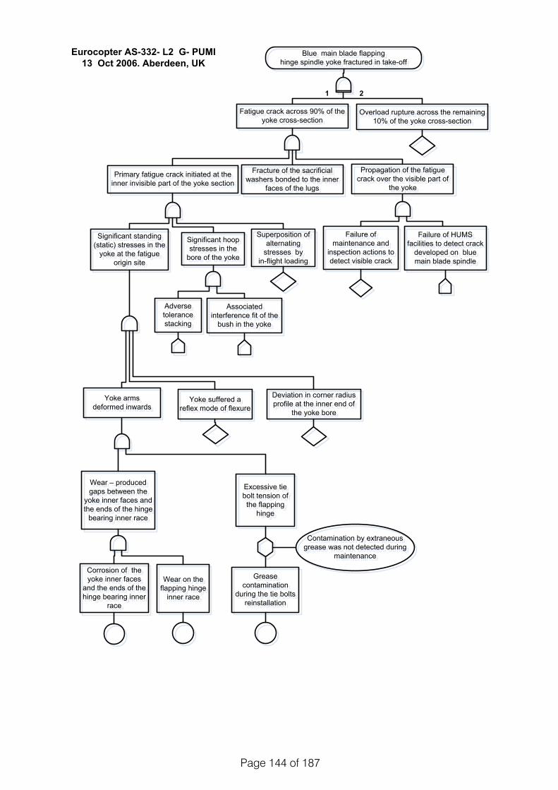
Page 144 of 187
Blue main blade flapping hinge spindle yoke fractured in take-off
Blue main blade flapping hinge spindle yoke fractured in take-off
Excessive tie bolt tension of the flapping
hinge
Excessive tie bolt tension of the flapping
hinge
Eurocopter AS-332- L2 G- PUMI13 Oct 2006. Aberdeen, UK
Fatigue crack across 90% of the yoke cross-section
Fatigue crack across 90% of the yoke cross-section
Wear – produced gaps between the
yoke inner faces and the ends of the hinge
bearing inner race
Wear – produced gaps between the
yoke inner faces and the ends of the hinge
bearing inner race
Wear on the flapping hinge
inner race
Wear on the flapping hinge
inner race
Corrosion of the yoke inner faces
and the ends of the hinge bearing inner
race
Corrosion of the yoke inner faces
and the ends of the hinge bearing inner
race
Grease contamination
during the tie bolts reinstallation
Grease contamination
during the tie bolts reinstallation
Fracture of the sacrificial washers bonded to the inner
faces of the lugs
Fracture of the sacrificial washers bonded to the inner
faces of the lugs Primary fatigue crack initiated at the
inner invisible part of the yoke sectionPrimary fatigue crack initiated at the
inner invisible part of the yoke section
Failure of maintenance and
inspection actions to detect visible crack
Failure of maintenance and
inspection actions to detect visible crack
Failure of HUMS facilities to detect crack
developed on blue main blade spindle
Failure of HUMS facilities to detect crack
developed on blue main blade spindle
Overload rupture across the remaining 10% of the yoke cross-section
Overload rupture across the remaining 10% of the yoke cross-section
1 2
Significant standing (static) stresses in the
yoke at the fatigue origin site
Significant standing (static) stresses in the
yoke at the fatigue origin site
Significant hoop stresses in the
bore of the yoke
Significant hoop stresses in the
bore of the yoke
Propagation of the fatigue crack over the visible part of
the yoke
Propagation of the fatigue crack over the visible part of
the yoke
Superposition of alternating
stresses by in-flight loading
Superposition of alternating
stresses by in-flight loading
Yoke arms deformed inwards
Yoke arms deformed inwards
Yoke suffered a reflex mode of flexure
Yoke suffered a reflex mode of flexure
Deviation in corner radius profile at the inner end of
the yoke bore
Deviation in corner radius profile at the inner end of
the yoke bore
Contamination by extraneous grease was not detected during
maintenance
Contamination by extraneous grease was not detected during
maintenance
Adverse tolerance stacking
Adverse tolerance stacking
Associated interference fit of the
bush in the yoke
Associated interference fit of the
bush in the yoke
!!

145
Annexe 3 - Primary and secondary fai lures and faults found using Fault Tree analysis of the selected hel icopter MGB and Main Transmission accidents and incidents
S
Case Description Primary failures / faults
Secondary failures / faults External qualifiers HUMS / IHUMS
Involvement
1 G-REDW
Loss of drive to MGB main lubricating system oil pumps due to 360° circumferential crack, in the bevel gear vertical shaft in the helicopter’s main gearbox, and later failure of the emergency MGB lubrication system.
Small corrosion pit 60 µm deep in the inner countersink of the 4.2 mm hole on the bevel shaft’s joining weld end point. Small machining defect in the internal part of the 4.2 mm hole. Other failures suspected as well.
Fatigue crack ‘A’ around 250° of the shaft circumferential weld joining upper and lower parts of the shaft.
Manufacturing defect suspected – investigation on-going.
HUMS data indicated higher vibration of the vertical bevel shaft of MGB at 6 flying hours before start of the accident flight. Prior to these 6 hours, the vibration levels on indicators associated with the bevel gear vertical shaft were below the main level established from data collected from 23 other helicopters of the same type. During the last 6 flying hours the vibration indications collected increased. An amber alert was generated after the last flight the day before the accident, and after the first flight of the accident day. Required maintenance actions were conducted as per the maintenance manual. Aircraft was placed on a 10 hourly close monitoring cycle and released for flight.
Fatigue crack ‘B’ around 80° of the shaft circumferential weld.
Manufacturing defect suspected – investigation on-going.
Crack ‘C’ around 30° of the shaft circumferential weld starting from crack ‘A’ and going under crack ‘B’
Undetermined – investigation on-going.
Total Circumferential failure of vertical bevel gear shaft at the circumferential weld.
None
Vertical down movement of the lower vertical bevel gear.
None
Damage of outer race of bevel shaft lower roller bearing.
None
Pinion partially disengaged from oil pump drive gear.
None
Damage of teeth of pump drive gear.
None
Failure of drive to main and standby oil pumps.
None
Undetermined MGB emergency lubrication system failed (MGB EMLUB caption came on)
Undetermined – investigation on-going.
! !

146
2 G-REDL Failure of one of the eight second stage planet gears in the epicyclic module as a result of a fatigue crack, the precise origin of which could not be determined. This led to the MGB outer case fracture and main rotor separation.
A crack had initiated from a point at or close to the surface of a highly loaded section of the bearing outer race in one of the second stage epicyclic planet gears of the MGB. A particle had been released from a position approximately 14 mm from the edge of the outer race of the failed gear Spalling of the planet gear. material defect within the gear (suspected).
Crack propagated under fatigue until the gear failed and broke into several sections.
The AS332 L2 does not provide an alert to the flight crew when the epicyclic module magnetic chip detector detects a particle. The ring of magnets, introduced on EC225 MGBs. reduced the possibility of detection of metallic debris, generated in the epicyclic module, by the main module magnetic chip detector or by inspection of the oil filter. Many other external technical and human inputs
HUMS recorded 667 epicyclic magnetic chip detection warnings 6 days prior to accident. These were not investigated due to the absence of an alert generated by the HUMS ground station. Alerts will not be displayed on the HUMS ground station summary screens, if the HUMS data card is not closed down correctly. HUMS recorded 76 chip detection warnings for the first operation of the day 6 days prior to accident, and 94 for the second operation. For both operations, the first recorded detection was during engine start. Three minutes and three seconds prior to the loss of MGB oil pressure, HUMS recorded an epicyclic chip detection warning. Three further detections were recorded over the next minute and 43 seconds. Review of HUMS vibration data available at the time of the accident revealed no unusual trends related to the epicyclic module. HUMS vibration monitoring capability of detecting degradation in epicyclic stage planet gear bearings is limited.
A section of the failed second stage epicyclic planet gear becomes entrained between the remaining second stage planet gears and the ring gear.
None
Rupture of the MGB epicyclic module case due to overload. This case is integral with the epicyclic ring gear.
None
Loss of MGB oil pressure. None Extensive leak (loss) of MGB oil.
None
MGB conical housing separated from the remainder of the MGB.
None
Lift struts reacted engine torque, thus fractured under load.
Lift struts were not designed to react engines torque
Separation of the main rotor None
! !

147
3 C-GZCH Total loss of MGB oil due to fracture of titanium studs securing the MBG oil filter bowl. This led to the failure of the MGB.
Galling of the titanium studs
Fracture of first stud.
Increased removal / installation cycles of studs. Improper pre-load installation of studs during maintenance. Increased cyclic loads on studs during flight.
HUMS data from helicopter is downloaded every day and used to monitor the helicopter's systems for faults or to detect trends that could lead to faults. However, the accident final formal report doesn’t list any specific HUMS data that could have helped indicating pending failures of oil filter bowl studs prior to accident flight. This could be attributed to the non-rotating nature of the filter assembly.
Fracture of second stud. Increased load on the 2nd stud after failure of 1st one. Increased removal / installation cycles of studs. Improper pre-load installation of studs. Increased cyclic loads on studs during flight.
Loss of MGB oil from oil filter bowl.
None
Plastic collapse of teeth of the tail take-off pinion (to tail rotor shaft).
Continued MGB operation after loss of oil.
Damage to two tapered roller bearings of the tail take-off pinion shaft.
Continued MGB operation after loss of oil.
Loss of axial and radial constraints of the main rotor brake disk.
Continued MGB operation after loss of oil.
! !

148
4 G-CHCF The right engine freewheel unit failed causing that engine to overspeed, this was contained by the overspeed protection system shutting down the engine, and the main rotor speed started to decay.
Wear of the freewheel shaft due to variations in the torsional loading and rigidity within the rotor drive system Freewheel unit roller cage rotated to a point where the rollers had overridden the freewheel ramps, and moved into the adjacent ‘trough’ in the freewheel shaft
The freewheel anti-rotation stops failed as a result of the roller cage rotating into them with significant force
Stops not designed to withstand significant increase of forces acting on them.
HUMS data for components with high rotational speeds, such as the engine input shafts, would be recorded more frequently than lower speed components, such as those within the main gearbox. At the time of the incident, data pertaining to the engine input shafts were recorded once every 20 minutes when the helicopter was in the cruise phase ONLY. HUMS detected progressive increase in vibration levels relating to the right engine input shaft 2 days before the incident, and following this engine replacement, these vibration levels had reduced. Both the helicopter manufacturer and operator concluded that the increasing vibration trend had been as a result of normal wear within the removed engine or its coupling to the main rotor gearbox and was not related to vibration of the freewheel unit. It can thus be seen that certain components, such as freewheel units, may not exhibit any detectable levels of vibration during normal operation and, as such, cannot be monitored effectively by a vibration monitoring system.
The shaft exhibited signs of significant mechanical wear on the ramps together with some burring of the ramp lips, produced when they had been ‘over-ridden’ by the rollers.
torsional loading and rigidity within the rotor drive system reacting on the freewheel shaft
Deformation and mechanical damage of rollers
None
Engine output shaft disengaged from the gearbox.
None
Engine overspeeded and automatically shutdown.
None
Misalignment of the torque sensing components.
Mechanical failure of freewheel shaft.

149
5 G-PUMI One main rotor blade spindle fractured through the lower section of its attachment yoke on the leading side of the spindle. Post-fracture plastic deformation of the lug had stretched open the fracture, separating the faces by some 12 mm.
Wear on the flapping hinge inner race Excessive clamping pre-load across the yoke (relatively tight-fitted pin) Significant hoop stresses in the bore of the yoke with the presence of interference fit. Smearing and parallel scoring aligned with the bore axis. These were produced by an interference fit between the bush and the yoke at the time the bush was installed.
Crack originated (258 flying hours before the incident) at the inner corner of the bore accommodating the flapping hinge pin.
Cracks were increased as the rotor centrifugal forces decayed and increased with each rotor stop/start cycle. The forces imposed by the lead-lag dampers were the most significant dynamic load variable (as distinct from the quasi-static centrifugal loading) influencing the yoke stresses at the fracture origin site. Trace amounts of grease had contaminated the tie bolt, introduced unwittingly as the tie bolt came into contact with extraneous grease in the bore of the flapping hinge pin, as the bolt was reinstalled.
IHUMS record did not detect any abnormal trend or condition occurred during the pre-accident recorded period, and during the post-accident flight testing, using the main rotor head components from the aircraft except the failed spindle. This confirmed that the load spectra used as basis for certification fatigue testing, and the fatigue tests themselves, were valid. Without specific sensors attached directly to the component, the onset of a crack, such as that found in G-PUMI, would probably not be detectable as the geometry of the blade would be unlikely to change sufficiently, until complete failure.
The spindle failed in fatigue, from that crack which propagated through the lower section of the lug on the ‘leading’ side of the yoke. The crack propagated through some 90% of the viable cross-section. The remaining 10% of cross-section failed in overload. The inner sacrificial washer had fractured radially along a path substantially parallel with the yoke fracture, but displaced some 5-11 mm from it. The washer was also fractured along a path on substantially the same chord line on the opposing arm of the lug. The fracture on the lower half of the washer displayed extensive post-fracture corrosion.
! !

150
6 G-JSAR Oil cooler drive shaft and gear wheel fractured, as well as the fracture of its bearing housing.
Transient torsional loads arising from 'snatching' in the gear train within the gearbox module.
The intermediate gear wheel fractured from the bearing at the centre to the outer edge of the gear.
None Prior to the accident, HUMS detected a potential problem in the main gearbox left hand accessory module. A decision had thus been made to monitor closely the relevant parameters (manufacturer advised to continue flying but with close monitoring for a further 50 flight hours), and the failure occurred during this monitoring period. The report notes that a similar incident occurred to G-PUMS.
Its bearing housing was also fractured through one of the three attachment lugs.
None
Oil cooler drive shaft fractured at the coupling flange on the MGB output drive.
None
7 C-FHHD
The plain bearing in the main gearbox cover for the number 1 input pinion failed, lost lubrication, and disintegrated. Engine 1 thus lost power.
The plain bearing in the main gearbox cover for the number 1 input pinion failed
The bearing adjacent carbon seal broke down.
None Not reported
Bearing lost lubrication (grease), and disintegrated.
None
The carbon seal for the failed plain bearing disintegrated
None
Oil spray out from the MGB on to the pinion shaft
None
The number 1 pinion rapidly overheated and weakened.
Continued MGB operation after loss of oil. Rotational imbalance due to bearing fracture.
Local fire started within the area (base of transmission)
None
Fracture of the No 1 pinion. None Malfunction of the No. 1 free wheel unit,
None
Engine 1 lost power None
! !
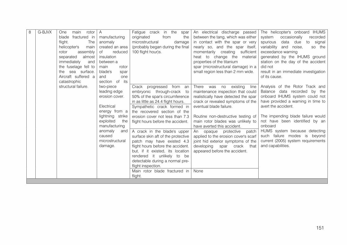
151
8 G-BJVX
One main rotor blade fractured in flight. The helicopter's main rotor assembly separated almost immediately and the fuselage fell to the sea surface. Aircraft suffered a catastrophic structural failure.
A manufacturing anomaly created an area of reduced insulation between a main rotor blade's spar and one section of its two-piece leading edge erosion cover. Electrical energy from a lightning strike exploited the manufacturing anomaly and caused microstructural damage.
Fatigue crack in the spar originated from the microstructural damage (probably began during the final 100 flight hour)s.
An electrical discharge passed between the tang, which was either in contact with the spar or very nearly so, and the spar itself, momentarily creating sufficient heat to change the material properties of the titanium spar (microstructural damage) in a small region less than 2 mm wide.
The helicopter's onboard IHUMS system occasionally recorded spurious data due to signal variability and noise, so the exceedance warning generated by the IHUMS ground station on the day of the accident did not result in an immediate investigation of its cause. Analysis of the Rotor Track and Balance data recorded by the onboard IHUMS system could not have provided a warning in time to avert the accident. The impending blade failure would not have been identified by an onboard HUMS system because detecting such failure modes is beyond current (2005) system requirements and capabilities.
Crack progressed from an embryonic through-crack to 50% of the spar's circumference in as little as 24.4 flight hours.
There was no existing line maintenance inspection that could realistically have detected the spar crack or revealed symptoms of the eventual blade failure. Routine non-destructive testing of main rotor blades was unlikely to have averted this accident.
Sympathetic crack formed in the recovered section of the erosion cover not less than 7.3 flight hours before the accident.
A crack in the blade's upper surface skin aft of the protective patch may have existed 4.3 flight hours before the accident. but, if it existed, its location rendered it unlikely to be detectable during a normal pre-flight inspection.
An opaque protective patch applied to the erosion cover's scarf joint hid exterior symptoms of the developing spar crack that appeared before the accident.
Main rotor blade fractured in flight.
None
! !

152
9 G-BBHM Engine 2 suffered rapid deterioration of the No 5 (location) bearing of the free turbine, causing failure of the adjacent carbon oil seal and mechanical interference between the Main Drive Shaft Thomas coupling and the Engine Mounting Rear Support Assembly tube, which completely severed the support tube.
High engine torque at rotor engagement, during three of the engine starts the day before the accident, two of which involved the No 2 engine. An increase in shaft vibration during the two-hour period preceding the accident.
Dynamic radial imbalance loading of the No 5 bearing (Engine 2) due to the onset of shaft vibration in the last two hours of operation.
None As per date of report: Interrogation of the IHUMS data held by the operator showed that data from the previous flight had not downloaded. The measured and recorded data suggests that, up to about two hours before the accident, vibration levels were normal. During the two hour period before the accident, the recorded data showed evidence of a developing anomaly. The need to check the successful download of the HUMS data set is an additional manual task which was unknown to engineering staff at the time of the accident (2002), although this is now conducted on a per flight basis. There is no requirement for data links between ground stations to facilitate the comparison of parameters across a fleet. Substantial operator intervention can be required During data acquisition, the flight crew currently have no indication of when the data acquisition process is complete. The instruction to crews to operate for sufficient time to acquire a full set of IHUMS data is an additional operational burden.
Free play (wear) in the No 5 bearing.
None
The No 5 bearing worn excessively and suffered cage failure in flight.
None
Power turbine shaft lost location and started to ‘orbit’.
None
The ‘live’ and ‘dead’ oil jet assemblies of the No 2 engine both experienced fatigue fractures of the rear oil tube in flight.
None
The Thomas coupling at the forward end of the MDS of the No 2 engine severed the EMRSA tube
Heavy rotational rubbing contact mechanism.
Damage to the free turbine shaft assembly of the No 2 engine, and associated MDS.
None
An intense in-flight fire occurred which affected flight control and other systems in the MGB bay.
None
! !
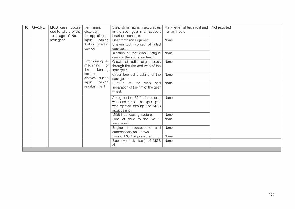
153
10 G-ASNL MGB case rupture due to failure of the 1st stage of No. 1 spur gear .
Permanent distortion (creep) of gear input casing that occurred in service Error during re-machining of the bearing location sleeves during input casing refurbishment
Static dimensional inaccuracies in the spur gear shaft support bearings locations.
Many external technical and human inputs
Not reported
Gear tooth misalignment Uneven tooth contact of failed spur gear.
None
Initiation of root (flank) fatigue crack in the spur gear teeth.
None
Growth of radial fatigue crack through the rim and web of the spur gear.
None
Circumferential cracking of the spur gear .
None
Rupture of the web and separation of the rim of the gear wheel.
None
A segment of 60% of the outer web and rim of the spur gear was ejected through the MGB input casing.
None
MGB input casing fracture. None Loss of drive to the No 1. transmission.
None
Engine 1 overspeeded and automatically shut down.
None
Loss of MGB oil pressure. None Extensive leak (loss) of MGB oil.
None
! !

154
11 9M-SSC The break-up of the second stage planet gear of the MGB. And break out of tail boom.
Seizure of roller bearing associated with secondary stage planet pinion (gear).
Gross contamination of the main gearbox magnetic plug and filter had occurred during the six weeks preceding the accident.
Mistaken health monitoring of the gearbox, leading to a deterioration of the mechanical condition of the gearbox components. Maintenance personnel had wrongly interpreted the amount of allowable debris as defined in the Aerospatiale Standard Practices Manual, due to the mistaken interpretation of an unfamiliar metric term.
The epicyclic module was not equipped with a detector.
Disintegration of a secondary stage planet pinion [gear] within the gearbox.
None
The associated metal debris caused jamming within the rotating assemblies, generating forces which fractured the common epicyclic ring gear and the main gearbox.
None
Circumferential failures of the ring gear casing, above and below the epicyclic stages, together with a vertical rupture.
None
Loss of the main rotor assembly, together with the attached bell housing containing the second stage gears of the epicyclic gearbox.
None
This resulted in the gross instability in the rotor system, which caused blades to strike the fuselage.
None
Almost simultaneously, the entire tail boom section parted from the aircraft.
None
! !

155
12 LN-OPG Fatigue cracks in
the splined sleeve of the R/H shaft input of the MGB, led to series of mechanical failures that caused the power turbine section of the R/H engine to burse, thus disintegrating the aircraft in flight. Whole sequence of the incident continued for only 3.9 seconds.
The hard metal coating of the splined sleeve containment was of larger carbide grains than the thickness of coating. Thickness of coating is less than the design requirements in some parts. Porosity of the coating is significantly larger than required by design. Local lamination of the hard metal coating. Defective bonding
Several fatigue cracks on the splined sleeve of the R/H shaft input of the MGB started 121 to 62 flying hours prior to accident.
None A IHUMS accelerometer with an ‘alarm’ that monitored the problem area was out of operation at time of accident (since 2 months before). It is concluded that adequate operation of this accelerometer would have given enough warning prior to the accident. The working parts of the IHUMS indicated a problem within the R/H engine and MGB connection area few days before the accident. This information remained saved in the associated database and had to be manually decoded to expose the trend of the problem. This was not conducted. The installation of IHUMS was on voluntary basis, thus some parts of it were occasionally left out of use.
Failure of the splined sleeve Missing O-ring on the splined sleeve increased freedom of movement between splined sleeve and splined flange, thus hastened the crack propagation on the splined sleeve.
Loosen locking washer slipped into the power transmission Bendix shaft of R/ H engine.
Design shortcoming of shaft.
Failure of the Bendix shaft under large imbalance loads
Inadequate maintenance procedures. Significant maintenance errors (missing O ring, inaccurate pre-flight checks, inadequate documents updates and signatures, etc.) Inaccurate and incomplete inspections
Increased onset of vibration s on the R/H engine
None
Failure of engine speed regulating controls
None
R/H engine overspeed out of control
Engine was freed of load due to Bendix shaft failure

156
between hard metal and coating
Engine power turbine burst None Fracture of two flight rod controls to the main rotor
None
Fracture of one rod control to the tail rotor
None
Destruction of power turbine section of the L/H engine
None
Front suspension bar of the MGB failed in overload
None
Main rotor head damaged and disintegrated.
None
!

Page 157 of 187 !
Annexe 4 - Fai lure Modes Analysis of the Helicopter Gearbox
Introduction
With maintainability and reliability now being a major concern in the development of the helicopter gearbox, good maintenance practice and high reliability can be achieved by developing techniques for a health monitoring system; this system diagnoses the fault prior to failure and predicts the remaining time before failure. Practically, root cause failure analysis is used to minimize design defects, identify potential hazards, and design the monitoring system.
Failure analysis was performed to identify the root causes of failure in the helicopter gearbox as well as the effect of the failure on the system’s health. The study also considers symptoms analysis and utilization of these symptoms in the health monitoring system.
The gearbox considered in this study is the gearbox of the Eurocopter AS332 L2 Super Puma, and the internal configuration of the gearbox is shown in Figure A4.1. The gearbox consists of two stages planetary gears, and one stage bevel gear.
!Figure A4.1: Gearbox internal parts [1]
The planetary gears are composed of 8 planet gears meshed to the sun and ring gears and the ring gear is fixed on the housing. For each planet gear, a roller element bearing is attached to the inner ring of the gear. The configuration of the gear is shown in Figure A4.2 and Figure A4.3 [1].
The oil system of this gearbox was modelled as a basic lubrication system as described in [190].

Page 158 of 187 !
!Figure A4.2: Planetary stages of the gearbox [1]
!Figure A4.3: Planet gear and bearing assembly [1]
! !

Page 159 of 187 !
The definitions of the important terms used in this study are summarized below.
Table A4.1: Definition of terms [191]
Term Defin i t ion
Cause The fundamental reason for a failure mode, which may see the physical degradation or the process leading to a failure mode. A cause can relate to design, manufacture, environmental, operational or maintenance actions, or an input flow that exceeds specified limits.
Component The assembly of parts grouped together to perform a common function/s.
Failure Effect The consequence of a failure mode on the functional output of a component, sub-system or system level. Failure effects are classified as local, next higher level, and end.
Failure Mechanism The chemical, electrical or mechanical process which causes the physical degradation of a system element and results in a fault.
Failure Mode The observable manner in which a system or system element fails to fulfil its function, expressed in terms of the deviation of its output flow from the specified or nominal limits. The failure mode results either from a physical degradation process within the system/system element or as a result of an erroneous input flow received from another failed system/system element.
Fault The physically degraded state of a system element (static) or a change in its behaviour (dynamic) which will result in a failure mode.
Part The lowest possible level of hierarchy in MADe. Parts comprise of individual physical units that are assembled to create a component.
Symptom The response of a failed system element that can be used to detect a failure mode, or a loss generated by a failure process that can be used to detect a failure mode.
System A grouping of sub-systems or components which interact to fulfil a common function.
!

Page 160 of 187 !
Model descript ion
The model was built in MADe environment. One of the great benefits of using this software is the utilization of the knowledge-base of the parts failures and this allows use of previous experience in failure analysis. This knowledge-base covers all failures that can be generated during the system operation. Therefore, this kind of modelling is used to optimize the diagnostic system and identify the best way to monitor a machine’s health.
The model structure is composed of two levels; the higher level is the components and the lower level is the parts. The component is a group of parts connected together to perform a certain function. A Part is the lowest level element on a System Structure Diagram. Parts in MADe cannot be directly modelled dynamically or functionally. Instead, they are joined with other Parts to form Pairs. A Pair is the connection between a Part and another Part. A pair defines how the two elements are joined, and can be assigned functions so that it may be included in Functional Analysis. In this study, two main components are considered and these are the gearbox and the oil system as shown in Figure A4.4 below.
Figure A4.4 - Model components
Each component is composed of many parts arranged according to the detailed drawing of each component. The gearbox consists of single bevel stage and two stages of planetary gears. In addition, bearings, shafts, seals, carriers, and the housing are considered in the gearbox model as shown below.

Page 161 of 187 !
Figure A4.5: Parts structure of the gearbox parts
Similarly, the oil system consists of many components including the oil sump, valves, the pump, the cooler and the filters. The system details are shown below and these components are arranged together to represent the function of the oil system.
Figure A4.6: Oil system components
The system function is built by selecting MADe library components and linking them to create a block diagram. The link represents the functional relation between components and these links are used to propagate the flow through the system. In the case of a failure of function, the failure is propagated through the system model by the functional links which warn the input and output flow of each component depending on the component level as will be illustrated later in the failure diagram.

Page 162 of 187 !
The function defined for the gearbox is as follows: the input and the output are the mechanical rotation and in addition the liquid oil and contamination is modelled as the input and output of the gearbox. The gearbox function definition is shown in Figure A4.7 below.
Figure A4.7 Function definition of the gearbox
The oil system’s primary function is circulation of the oil, contamination elimination and heat dissipation. The inputs are modelled as mechanical rotation to rotate the pump, the liquid oil, and the contamination from the gears. In the same way, the outputs are oil and contamination. The contamination output is modelled as a special case occurring when bypass line is used and oil filters is out of operation. For this reason, the oil contamination is modelled as input to the gearbox, because in this case the contamination can be circulated between the gears and the oil system. The layout of the oil system considered is shown below.
Figure A4.8 - Basic lubrication system [190]
After the function is defined for each component, the next step is to define the failure path and link failure to the function of each component. The failure diagram consists of four levels: Causes, Mechanisms, Faults, and Symptoms. The faults are connected to the part/system/component function depending on the type of fault. For example, some faults only cause failure of the parts function and the component continues to perform its function. An example of a failure diagram for one gear part is shown in Figure A4.9 below.

Page 163 of 187 !
Figure A4.9 - Failure diagram
The failure diagram is connected to the function depending on the faults’ effects. In some cases, the effect is only limited to the pairs of parts in connection, and sometimes the faults are related to the system function. An example of two cases is shown below.
Figure A4.10 - Pairs fault to function relationship

Page 164 of 187 !
Figure A4.11 - Failure connections to system function
The model is based on the assumption that all the failure paths have the same probability of occurrences. This probability will be used as contribution estimation on each fault of the gearbox failure, and will identify the strongest way to detect a fault based on the system symptoms analysis.
Calculat ion Example
Due to the complexity of the probability estimation in the model, a simple example is presented to demonstrate the concept. The calculation is used to determine the probability of occurrences of faults, symptoms and mechanism causes [192]. In the failure diagram shown in Figure A4.12, each item has a probability score of 10; this probability is defining the likelihood or frequency with which the cause generates the effect. The probability is ranked from 1 to 10 with 1 being very low and 10 being very high [193].
According to this example, there are three failure scenarios as follows:
Insufficient lubrication – abrasive wear – fracture;
Impact load – impact fracture – partial crack;
Impact load – impact fracture – fracture.
These scenarios have the same probability. However, the fracture fault appears in two failure paths and therefore the fracture fault occurrence can be estimated as 66.66% of the faults in this model, and partial crack is 33.33%.
In the same way, symptoms can be analysed. The symptoms analysis is based on finding the symptom leading to the detection of the majority of failures. In this example, two symptoms are presented: solid debris and change of behaviour. The latter can identify the occurrences of two faults in this model, whereas solid debris can detect only one fault. Therefore, the change of behaviour symptoms leads to the detection of 100% of faults, while oil debris detects 50% of faults.
This type of analysis highlights the major area of interest for monitoring and fault diagnostics. In addition, failure causes and effect can be studied to help both designers and operation and maintenance staff.

Page 165 of 187 !
Figure A4.12 - Simple example of failure diagram
Result and discussion
By including component hardware details and defining the operating condition, the model is generated; this model can be used to determine system monitoring requirements and to estimate the best way to design the Fault Detection and Isolation (FDI) system.
Model analysis shows that the top cause of failure is the solid debris existence in the lubricant as shown in Figure A4.13. Also, high load, insufficient lubrication and corrosive contamination contribute significantly as failure causes.
Figure A4.13 - Top causes of gearbox failure

Page 166 of 187 !
The causes result above leads to the generation of a failure mechanism shown in Figure A4.14. The main failure mechanism is abrasive wear and this coincides with the main cause of failure which is oil debris. This cause leads to the generation of the abrasive wear mechanism. The mechanisms such as cavitation corrosion and pitting, in addition to abrasive wear, contribute to 50% of mechanisms leading to failure.
Figure A4.14 - Top failure mechanisms in a gearbox
The faults generated from failure mechanisms are shown in Figure A4.15. It is obvious that the parts fracture is the common fault in this failure model. This is due to the fact that if the mechanism progressed this would lead to failure. In addition, it is due to the progress of some faults until part fracture and an example of this type of fault is cracks.
Figure A4.15 - Percentage of faults contribution from failure path
The diagnostic set of faults is a list of symptoms that can be used to uniquely identify the fault. The model generates the symptoms related to these faults and estimates the symptoms ranking as shown in Figure A4.16. In this figure, symptoms leading to fault detection are estimated. According to the result, the solid debris symptom is the strongest symptom leading to fault identification. Therefore, solid debris should be used as a monitoring technique to identify the faults in the gearbox. This result shows there are no unique symptoms which can lead to the identification of all faults. For this reason, a combination of monitoring techniques can lead to a stronger monitoring system. Symptoms analysis proves that using solid debris, surface change, behaviour change, performance, shape and vibration, results in the coverage of 85% of faults. Acoustic emission would fall under these categories. In these proposed techniques surface and shape change can be achieved by strain monitoring.

Page 167 of 187 !
Also, the change of behaviour monitoring is achieved by monitoring angular speed variation, and the performance monitoring is achieved by torque monitoring.
Figure A4.16 - Faults percentage covered by symptoms
Also, symptoms of faults in the oil system can be estimated from the model. According to this result, shape and surface change are the top symptoms to detect the failure. However, these two symptoms can be applied in visual inspection. Therefore, performance parameters such as oil pressure and solid debris can be used for online monitoring.
Figure A4.17 - Percentages of faults covered by symptoms in lubrication system
Conclusion
This report has outlined the failure analysis of the helicopter gearbox. This analysis is aimed at optimizing the system monitoring design and developing model based diagnostics. Statistical estimation was performed in the model to find the failure paths of the gearbox and the estimation concludes the following points:
• Solid debris in oil lubrication is the main cause of failure and it leads to the abrasive wear mechanism;
• Monitoring of solid debris is the best way to monitor the faults in the gearbox and faults can be detected early before any other fault symptoms;

Page 168 of 187 !
• There is no unique symptom result in detection of all faults and therefore a monitoring combination can produce a more reliable diagnostic system;
• The fault monitoring design should consider the economical side of monitoring techniques. Therefore, performance and velocity monitoring are considered to be the cheapest techniques due to the use of existence measurement of the control system;
• According to this study, the techniques proposed for helicopter gearbox monitoring are:
o Oil solid debris
o Torque and angular velocity
o Strain gauges (wireless)
o Vibration
o Acoustic emission
! !

Page 169 of 187 !
Annexe 5 – Transmission testing
Background noise was measured to of the order of 0.005 (5mV)
!!
!!
!Peak value of 9.99V (full deflection) = 2000x
!Figure A5.1 - Pencil lead break on end: position, time data and zoomed time data

Page 170 of 187 !
!
!!
!Peak value of 9.99V (full deflection) = 2000x
!
!!
Figure A5.2 - Pencil lead break on shoulder: position, time data and zoomed time data
! !
0 2 4 6 8 10 12 14x 106
−10
−8
−6
−4
−2
0
2
4
6
8
10
6.5 7 7.5 8 8.5 9 9.5 10 10.5 11x 106
−2
−1
0
1
2
3

Page 171 of 187 !
!!!!
!!
!Peak value of 4.8V = 1000x
!
!!
Figure A5.3 - Pencil lead break on roller: position, time data and zoomed time data
5 6 7 8 9 10 11 12 13x 106
−5
−4
−3
−2
−1
0
1
2
3
4
5
8 8.5 9 9.5 10 10.5 11 11.5x 10⁶
−1.5
−1
−0.5
0
0.5
1
1.5

Page 172 of 187 !
!
!!
!Peak value of 3.3V = 500x
!Figure A5.4 - Pencil lead break on outer race of furthest bearing (inner bearing properly located):
position, time data and zoomed time data
0 0.5 1 1.5 2 2.5x 10⁷
−4
−3
−2
−1
0
1
2
3
4
0.8 0.85 0.9 0.95 1 1.05 1.1 1.15 1.2 1.25 1.3x 10⁷
−0.8
−0.6
−0.4
−0.2
0
0.2
0.4
0.6
0.8

Page 173 of 187 !
!!
!Peak value of 3.2V = 500x
!!Figure A5.5 - Pencil break on gear tooth (both bearings assembled and lockring installed):
position, time data and zoomed time data
0 0.5 1 1.5 2 2.5 3x 10⁷
−4
−3
−2
−1
0
1
2
3
4
1.18 1.2 1.22 1.24 1.26 1.28 1.3 1.32x 10⁷
−0.3
−0.2
−0.1
0
0.1
0.2
0.3

Annexe 6 – Circuit diagrams
Figure A6.1 - Crystal oscillator, buffer amp and power amplifier (fixed part)
+5V
+12V
+12V
RF1SMA1
Vcc4 out 3
gnd
2
EN1
X1GXO 7551
C21100n
R17390
R18300 Q1
BFS17
R1956
C22100n
C23
100n
Tx outputQ2IRFD110
TP3
TP2MM
TP4
TP2MM
C34100n R31
10k
C3510n
C37
10nR3210
32
1
VR15k
5Vpp
2.5Vpp
150 mA
C45
100n
R374k7
R382k2
C131u4.5t on 144nH/t2
2.5Vpp on a 3V bias
R39270

Page 175 of 187 !
Figure A6.2 - Coherent demodulator, filter and output amp (fixed part)
+8V2
+8V2
sigin1
gain12
gain23
sigin-4
bias5
op+6
nc7
Vee 14
nc 13
op- 12
nc 11
cin- 10
nc 9
cin+ 8
U3MC1496
R51k2
R6820
R71k
C71u
C81u
C91u
R8
680
R9120
R10120
R1110k
R122k7
C10100n
R132k7
R14
2k7C11100n
C12100n
Coherent AM demodphase shifter
C2710n
J1SMA1
Receive input
R2251
R23LK
R24NF
3
26
4817
5
U5 AD8021
C291u
C3010p
R25
3k3
R26220
R2810k
R2910k
R3010k
C311u
C32100n
C33100n
J2SMA1
Baseband output
R33100
R341k
R16100
C362n2
C404n7
L810u
L910u
C412n2
1.1 MHz LPF + buffer
C424n7
L1010u
R2710k
Q3BFS17
R35100
C43100n R36
33k
C44100n
C2433p
C2533p
L7
820nH
C26100n C46
100n
R151k
Av = 160.75Vpp
0.75Vpp
carrier
R20100
R21
51
C14470p
C15680p
C16680p
C17470p

Page 176 of 187 !
Figure A6.3 - Rotating coil rectifier, buffer amp and varactor modulator
TP1
TP2MM
TP2TP2MM
D1
BAT54
D2
BAT54
C14u7
C210n
D3BB148
C368p
3
41
52
U1
LMP7715MF
R110k
R24k7 R3
2k7R4220
C4100n
R5
10k
C5100n
TP3
TP2MM
At HF, gain = 1+2k7/220 = 12.3
At dc, gain =1
C7100p
C8120p
R7220
1.05Vdc
L1
6800n
L2
6800n
C9150p
*
*

Page 177 of 187 !
Annexe 7 - Chips produced during testing
Figure A7.1 - Index of chips produced during major damage test
Figure A7.2 - Image 10

Page 178 of 187 !
Figure A7.3 - Image 11
Figure A7.4 - Image 12
Figure A7.5 - Image 14
Figure A7.6 - Image 15

Page 179 of 187 !
Figure A7.7 - Image 16
Figure A7.8 - Image 18

Page 180 of 187 !
Figure A7.9 - Image 19
Figure A7.10 - Image 20
Figure A7.11 - Image 21

Page 181 of 187 !
Figure A7.12 - Image 22
Figure A7.13 - Image 23
Figure A7.14 - Image 24
!

Page 182 of 187 !
Annexe 8 - Investigation of the nul l response
During testing, a periodic dead zone was noted in the output from the receiver. It was present under most testing conditions of the gearbox, but not at very low speed/torque settings. Attempts were made to recreate the dead zone away from the gearbox and bench, both in the electronics and also in the sensor.
Possible explanations of the null response include:
• overload of the electronics by very strong low frequency pulses from the sensor;
Large amplitude inputs, resulting in a full deflection square wave, subsequently low pass filtered, could give the time trace seen in the testing
• nonlinear response from the sensor from high amplitude vibration;
The very high amplitude, low frequency vibration seen at the planet carrier, could cause excessive strain in the sensor, causing it ‘saturate’ in some way and cease responding
• static build-up on the sensor.
These three possibilities were addressed in turn.
A8.1 Electronics over load
The first test was to drive the sensor board with a small HF signal at 250 kHz and superimpose a large lower frequency pulse. To do this, two signal generators were combined, one producing a constant small level sine wave at 250 kHz and a second producing a 500 Hz half sine pulse of much higher amplitude. They were fed to the sensor board which was set up as used in the full-scale testing, i.e. mid gain of 6x.
Firstly, the equipment was set up and validated by performing a 2 kHz to 1 MHz sweep. The sensor was then driven with a large sine signal to check behaviour under overload conditions. It was well behaved and went into ‘graceful’ clipping without any undesired effects or instability.
Figure A8.1 - Onset of clipping

Page 183 of 187 !
Clipping occurred at an input level of 520 mV input at which point the output was seen to be 2 Vpp. The output from the MGB on the test bench was in the region of 500 mVpp, which is well within the headroom of the opamp buffer.
Now the dual signal was applied. The half sine overload pulse is shown with underlying 250 kHz ripple (which is difficult to visualise on the oscilloscope output):
Figure A8.2 – 500 Hz half sine pulse with underlying 250 kHz sine wave
As the level of the half sine pulse was increased, the output of the system was inspected carefully, for any signs of instability. Figure A8.3 shows the 250 kHz tone at the peak of the half sine pulse, applied at 1 V peak. There are no visible effects.
Figure A8.3 - Output under overload pulse conditions

Page 184 of 187 !
The 500 Hz sine wave was increased into gross overload and possibly near the damage level of the opamp and the following trace was recorded:
Figure A8.4 - Output under gross overload with 500 Hz sine input
There are no unexpected results, but there is some evidence of the 500 Hz signal breaking through the high pass filter.
A8.2 Vibrat ion source
Next it was decided to see whether the dead zone could be replicated by driving the sensor with some high levels of vibration. To do this, a sensor was fitted to a brass block and excited by several means:
Figure A8.5 - Exciting sensor with a tungsten carbide “ball” bit, abrasive wheel and centre punch
The carbide bit was metal and it was thought the metal-to-metal contact might generate electrical noise, so the bit was replaced with a non-conducting grinding wheel. The centre punch produced
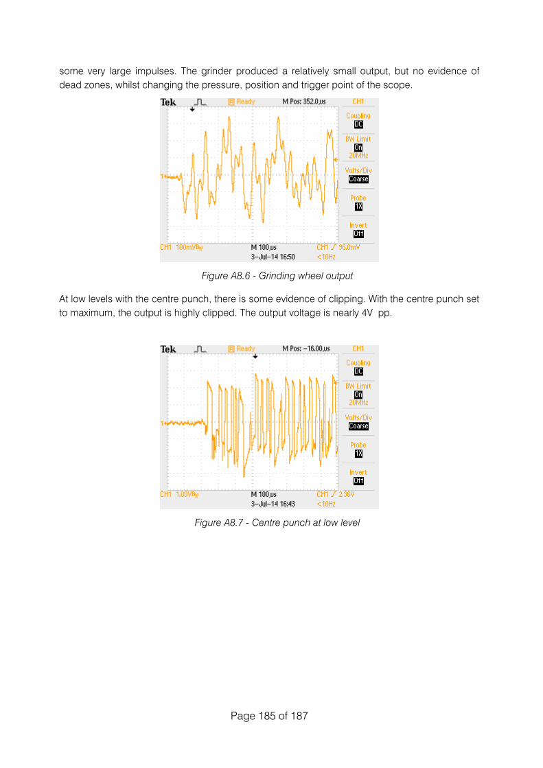
Page 185 of 187 !
some very large impulses. The grinder produced a relatively small output, but no evidence of dead zones, whilst changing the pressure, position and trigger point of the scope.
Figure A8.6 - Grinding wheel output
At low levels with the centre punch, there is some evidence of clipping. With the centre punch set to maximum, the output is highly clipped. The output voltage is nearly 4V pp.
Figure A8.7 - Centre punch at low level

Page 186 of 187 !
Figure A8.8 - Centre punch at high level
The exponential decay at the waveform peaks is due to the high pass filtering applied at the input of the sensor board. The system cannot pass DC, so we obtain the characteristic RC decay.
A8.3 Stat ic discharge
A build up of static charge on the live side of the sensor might eventually lead to some polarising or biasing of the dielectric, until it broke down.
In this situation, the device would work initially, then static would build up and it would stop working until a breakdown relieves the electrical stress, resulting in an impulse. The device would then resume normal operation.
The static might not leak away as the input to the amplifier is AC coupled with a small 100pF capacitor.
There was no means of generating a static charge, however an electrical impulse from a piezo spark discharge did cause an impulse effect. However, the waveform from the grinder is still plainly visible as the output swings towards the negative supply:
Figure A8.9 - High voltage discharge near sensor
The dead zone has not been replicated by either gross electrical overload of the system or mechanical overload of the sensor.

Page 187 of 187 !
Overload would more likely produce an output that slewed to the supply rail voltage for a period of time. However, the observed response is actually a period of silence, rather than a high output. It is as though the sensor has ceased operation for a moment, the quiet period is always at 0 VDC. Also, the null period is often followed by a short pulse, sometimes of negative or positive excursion, which is not something that would be expected under overload conditions.
There is no preceding large pulse, or exponential edge, indicative of something coming out of saturation just before the event. Opamps can exhibit recovery times from gross overload.
The effect was noted on the scope (which has a wide bandwidth and goes down to dc) and on the data captured by the card. It is not caused by the acquisition system filtering.
If it was something to do with the rotation of the coils in the gearbox, one might expect to see a repeat rate of 4 Hz (rotational frequency). Instead, it appears at a much faster rate generally, about a few hundred Hz, although sporadically.
The conclusion drawn from this investigation is that the effect is probably not caused by overload that can be easily reproduced. The verified cause remains undiscovered, although later discussion with the manufacturer suggests that it may be some type of overload effect within the sensor although the mechanism is not clear.
It is interesting a similar effect has been noted before in 2001, from a sensor and preamp alone. The explanation given was that the amplifier preceding the high pass filter was driven into saturation. However, in our case, we have no active components before the high pass filter, which is a small value series capacitor.