Vertical Temperature Profiles in Rooms Ventilated by Displacement: Full-Scale Measurement and Nodal...

Indoor Air, 2, 225-243 (1992)

0 1992 Munksgaard, DK-Copenhagen

Vertical Temperature Profiles in Rooms Ventilated by Displacement: Fd=Scale Measurement and Nodal Modelling Yuguo Li’,3, Mats Sandberg and Laszlo Fuchs’

Abstract The vertical temperature profiles have been measured in a fill- scale o f i e room ventilated by displacement. Different wall radiative emissivities have been empluyed w study the effect of thamal radktion. The change of the vertical locations of the heat source does not affect the s t a t h a y front, but modifis the temperature profile.

Two new nodal models, i.e. a four-node model and a multi- node model, are developed for predicting the temperature pj i le based on the flow and t h l characterization in the room. Agreement between the models and the experiments are vey good. The calculated results are applied w show that the temperature profile is influenced consuierably by the heat c d u c - twn through the walls and the t h l radiation between the wall surfbces. % m&ls heloped can be used for design purposes, as well as to supply the thamal bouna!ay c d i h in a CFD code.

KEY WORDS: Displacement ventilation, Energy consumption, Indoor air quality, Nodal model, Thermal comfort, Temperature distribution.

Manuscript received: 21 April 1992 Accepted for publication: 6 October 1992 ’ Department of Mechanics/Applied Computational Fluid Dy-

nynamics, Royal Institute of Technology, S-100 44 Stockholm, Sweden National Swedish Institute for Building Research, Box 785, S- 801 29 Gavle, Sweden Present address: CSIRO, Division of Building, Construction and Engineering, PO. Box 56, Highett, Vic. 3190, Australia

’

’

Introduction Displacement ventilation has been proved to be more efficient than mixing ventilation in simultan- eously removing excess heat and achieving good air quality. The basic physical principle behind ventilation by displacement is based on the properties of stratified flow. There is both a density (thermal) stratification and a contaminant stratification in the room. The thermal and contaminant stratifications are not alike in spite of being generated by the same source. The contaminant stratification is sharp. Es- sentially the room is divided into two zones, a lower zone with “clean” air and an upper polluted zone. On the other hand, the thermal stratification does not show this pronounced discontinuity. The expla- nation of this difference is that heat is also transported by radiation transfer between room surfaces.

Figure 1 shows the essential features of a ventilation system by displacement. Ventilation air with a lower temperature (usually around + 19 “C) than the mean room air temperature is introduced at floor level, while the warm air is extracted at ceiling level. In order to avoid draught the air is supplied at low velocity through large “low velocity devices”. The type of flow discharged from low velocity devices is not of the jet type. The flow is, to a great extent, governed by the buoyancy forces causing the air to spread out on the floor in a thin layer. From the heat sources in the room, plume flows are generated. Heat and contaminants are transported by the plume into the upper part of the room. Thus, in the area outside the plume, a vertical temperature gradient and related density stratification are generated. This means that we achieve a stable stratification with lighter air floating above heavier air.

The ceiling is warmer than the other surfaces and this gives rise to radiation transfer fiom the ceiling mainly to the floor. As a result, this makes the floor warmer than the air layer adjacent to the floor and

226 Li et 01.: Vertical Temperature Profiles in Rooms Ventilated by Displacement: Full-Scale Measurement and Nodal Modelling

Height [ cm l

0 ', I 1 , I

15 16 17 18 19 20 21 22 2 Temp Is(

Fig. 2 Measured temperature profiles in a water model (Sand- berg and Lindstrom, 1990).

the ceiling cooler than the air layer below the ceiling. This in turn affects the aidow pattern and temperature distribution in the room. The radiation exchange primarily affects the velocities in the air stream from the supply device and the vertical temperature profile.

The velocities and temperature at floor level and the vertical temperature gradients in the room are all important comfort parameters. With ventilation by displacement there is a risk of cold discomfort for the legs and feet, in conjunction with heat discomfort at head height (Wyon & Sandberg, 1990). The vertical temperature gradient is a main factor that determines the maximum cooling capacity for displacement ventilation. Furthermore, knowledge concerning the vertical temperature distribution is important for correct control of the system and thereby energy consumption. One argument often put forward as an advantage of displacement ventilation systems is that they are believed to give rise to lower velocity fluctuations than jet controlled mixing ventilation.

The purpose of this paper is twofold:

0 to study the effect of radiation, wall conduction and the position of heat sources on the vertical temperature profiles; and

0 to develop new simplified models for predicting air and wall surface temperature profiles.

Previous Work In recent years, considerable experimental work has been done on temperature and contaminant disui- bution with displacement ventilation. In an effort to develop a simplified model for ventilation by displacement, Sandberg and Lindstrom (1987, 1990) have carried out measurements in a plexiglass cube with

Li et al.: Vertical Temperature Profiles in Rooms Ventilated by Displacement: Full-Scale Measurement and Nodal Modellina 227

water as a flow medium. Here the water temperature field is closely related to the stratified flow that oc- curs, and the surface radiative heat transfer that ex- ists in the room is suppressed. A typical water temperature profile is shown in Figure 2. The water temperature in the lower part of the vessel remains almost the same as the supply water temperature. Full-scale experiments have been performed by sev- eral authors, e.g. Sandberg (1985), Nielsen et al. (1988), Sandberg and Blomqvist, (1989), Heiselberg and Sandberg (1990), Mathisen (1990). Two examples of air temperature profiles and concentration profiles are reproduced in Figures 3 and 4. The concentration shows larger stratification than temperature with a sharp change at the stationary front. The similarity between the water temperature profile and the air concentration profile indicates the similarity of the pure convective and turbulent transport of scalar quantities.

In order to provide the crucial parameters which determine the performance of a ventilation system to designers, simplified models with differing levels of complexity have been developed, e.g. the filling box model of Sandberg and Lindstrom (1987) and the two-zone box models as reviewed by the authors. These models predict the transport of the contaminant in the air. A more complex approach is based on numerical solution of the Navier-Stokes equations with turbulence models. This has been performed by Davidson (1989). To include the thermal radiation effect, Chen and van der Kooi (1990) predict the indoor wall surface temperature disuibu- tion for a CFD code by indirect coupling with a cooling load code; this, in turn, uses the airflow pattern pre-calculated by the CFD code. The three dimensional CFD approach gives very detailed infor- mation, but it is still limited for design purposes because of its computational cost and lack of univers- ally applicable turbulence models. Numerous efforts have been directed at simplified modelling of thermal transport in a room, e.g. the model of Beier and Gorton (1978) for industrial displacement ventilation and the model of Mundt (1990,1991) for an office room with displacement ventilation. These two models predict the vertical temperature profile by considering convection and radiation. Thermal conduction through the walls has also been considered in the first model. The nodal approach developed by Mundt (1990) is closely related to zonal modelling (Howarth, 1983, Overby and Steen-Thgde, 1990, In- ard and Buty, 1991). The difference is that the nodal approach does not consider the convective transport

2.5 I I

" I I I I I I I

0 0.2 0.4 0.6 0.8 1.0 1-T, 1.2 - T e - 3

Fig. 3 Measured temperature profiles in a full-scale room (4.2 x 3.6 x 2.5 m3) with slender cylinder heat source (Heiselberg and Sandberg, 1990).

1 roornvolumes/h ------ * ~ . . - ---_ 3-,,-

4 ~ . , ~

............. 5-,.-

I 0 I I I +

0 0.2 0.4 0.6 0.8 1

Concentration

max.concentration

Fig. 4 Measured concentration profiles in a full-scale room (4.2 x 3.6 x 2.5 m3) with slender cylinder heat source (Heiselberg and Sandberg, 1990).

between zones. The model by Howarth (1983) does not consider radiation. The nodal approach can be done in displacement ventilation due to the fact that the convective transport between the core region and the gravity current is hindered by stratification. This is a fortunate characteristic in displacement ventilation, because one of the difficulties in the zo-


2 0.36 3 0.36 4 0.15 5 0.36 6 0.36

Fig. 5 The test room and its configuration.

nal models is the definition of airflows between zones. The nodal approach can be easily extended to include the non-uniformity of vertical wall surface temperature which is to be discussed later.

The air is supplied directly to the occupied zone with a low velocity flat terminal located on the rear wall at floor level, and the air leaves the room through an overflow device. The supply terminal is 0.5 m high and 0.45 m wide with a 50% degree of

Experimental Approach As a full-scale model of a common type of ofice room, the test room is located in a comer of a larger enclosure as shown in Figure 5. The test room is located within the Heating and Ventilation Labora- tory of the National Swedish Institute for Building Research. The test room has internal dimensions of 4.2 m in length, 3.6 m in width and 2.75 m in height. The larger enclosure is intended to control the air temperature on the three exterior surfaces of the test room. The U-values of the room walls can also be seen in Figure 5. The exterior surface temperatures of one of the vertical walls and the ceiling are thus influenced by the indoor thermal conditions in the laboratory. However, the fluctuation in air temperature inside the laboratory during the log- ging period was within 20.5 "C. All the interior wall surfaces are, depending on the experiment, ei- ther painted black or covered with a sheet metal of aluminium. The emissivity of the aluminium surface has been measured over a wavelength range of 2 to 40 pm. The emissivity at 9.5 pm is 0.1 (recorded by the Department of Solid State Physics at Uppsala University in Sweden).

perforation. Thus the total free opening area of the inlet is O.ll25 m2. The supplied air temperature is controlled to be within & 0.2 "C. The supply airflow is measured with an orifice plate. The exhaust outlet in the side wall consists of an overflow device with a dimension of 0.525 x 0.220 m2 and is located at a height of 2.5 m. A cubic porous heat source with dimensions 0.4 m x 0.3 m x 0.3 m is constructed for the convenience of the numerical calculation with the Cartesian grids. In total 24 bulbs of 25 W each are uniformly built into the cube, allowing different levels of heat load up to 600 W. The main frame of the cube is an aluminum net and the cube is filled with aluminium chips which is intended to give a more uniform distribution of the heat load and to reduce the short-wave radiation from the heat source to the wall surfaces. The distance between the floor surface and the bottom of the heat source is generally maintained at 0.11 m and the distance between the supply terminal and the heat source centre at 2.7 m.

The room is instrumented with 59 type-T (cop- per-constantan) thermocouples with a HP 3497A Data Acquisitiordcontrol unit. Thirty thermocouples are used to measure the vertical air temperature

Li et 01.: Vertical Temperature Profiles in Rooms Ventilated by Displacement: Full-Scale Measurement and Nodal Modelling 229

Table 1 Measured cases and their parameters

Case n E(W) TCC) TOsi TO*, Tm3 T**, TO$, Te Ar

B1 1 300 16.0 20.2 22.7 23.0 23.2 20.3 27.3 21.0 B2 2 300 19.2 20.3 23.1 23.3 23.0 21 .o 26.7 3.54 B3 3 300 18.0 19.8 22.5 22.8 22.6 20.0 24.8 1.43 B4 3 450 18.0 19.8 23.0 22.4 22.5 19.8 26.9 1.82 A2 3 300 18.0 20.1 22.7 22.9 22.8 20.3 25.0 1.50

with high resolution near the floor and the ceiling. Twenty-two thermocouples are used to measure the interior wall surface temperature with five located vertically on each wall and one for ceiling and one for floor. Five thermocouples are used to measure the exterior surface temperature of the four walls and ceiling and two thermocouples are used to measure supply and exhaust air temperature, respectively. The thermocouples for air are shielded by aluminium foil to minimize the effect of the long- wave radiation exchange. The wall surface thermocouples are attached to the surface with tape to provide intimate thermal contact with the wall. The measured error in temperature is estimated to be within 0.2 "C. In the tests with aluminium as the wall coating, the wall surface thermocouples are also shielded by an aluminium foil.

The velocity measurements are carried out with a Dantec 56C14 temperature-compensated bridge and a Dantec 55R76 fiber-film probe. The Johansson-Al- fredsson formula (Johansson and Alfredson, 1982) is used as the velocity calibration equation. The detail of the low velocity calibration procedure can be found in Li et al. (1992). A total number of 1024 x 32 samples have been collected. A 12 bit A D con- verter is used and the sampling rate is 100 Hz, giv- ing an integration time of 5 minutes. The signal is filtered at about 40% of the sampling frequency. A PDP 11 computer is used to control the receiving and storing of data from velocity and temperature transducers. The uncertainty of measurements of mean velocity due to the limited sampling period (5 minutes) is 0.7%.

The measurements are carried out under steady- state conditions. To achieve the steady-state condition, each experiment is allowed to run for about 12 hours between any two different supply temperatures, flow rates and heat load settings. The steady- state condition is indicated by a steady exhaust air temperature. The test conditions are listed in Table 1.

Thermal Characterization Accurate prediction of the vertical temperature profile is difficult because of the essential coupling between turbulent flow and thermal transport. As an internal or confined problem, the core region is par- tially or fully encircled by the primary streams; these are the gravity currents formed from the supply device, the thermal plumes generated over the heat sources and the boundary layers established near the solid surfaces. Due to this fact, the core flow cannot be analytically determined from the boundary conditions and the primary flow streams but depends on them. The primary streams are, in turn, modified by the core. The interactions among the primary streams and the core establishes the final vertical temperature profile. In order to develop a simplified model, the flow and thermal characteristics in the room have to be specified and certain simplifications have to be made to keep the domi- nant parameter.

The field is characterized by two important primary air streams, i.e. the flow from the supply device and the plumes over the heat sources. Recent studies by Sandberg and Mattsson (1991a and 1991b) show that the flow from the low velocity terminal in displacement ventilation is no longer of the jet type but is gravity current. The entrainment of ambient air into the gravity current is hindered by the thermal stratification. The flow rate in the current stays almost the same as the supply flow rate. This gives us the first and most important assumption in nodal models, i.e. that the convective heat transport between the gravity current and the ambient air can be neglected. As the gravity current advances along the floor, it is heated gradually by the convective heat transfer along the floor surface. As a consequence, the buoyancy force of the gravity current decreases gradually. This can be seen from the streamwise velocity profile in front of the supply terminal (see Figure 6). In the case with aluminium coating, the floor sur- bce is relatively colder. The gravity current is not wea- kened as much as the case with black walls.


2.0

n - 1.5

Wl

E z .3

i2 1.0

0.5

(mixing flow region)

-----------

(unidirectional

-

-

.

-

2.5

warm gravity current region

stratified region --.

Fig. 6 The streamwise velocity profiles near the floor in front of the supply device with two different wall surFace coatings.

Fig. 7 The three-zone assumption in the simplified nodal models.

0 - Air( aluminium walls ) A ...... Air( black walls ) 0 - Wall surf.( aluminium walls ) A .'--.- Wall surf.( black walls )

Fig. 8 Measured temperature profiles with two different wall

0 1 2 3 4 5 6 I surface coatings (cases 83 and A2 0.0

Temperature(T-Ts) ("C) in Table 1).


Fig. 9 Measured temperature profiles with different horizontal distance x h .

(300 W heat load, n = 3 and black walls). Temperature( T-Ts) ("C)

0 - Air(Hh=O.llm) A ...-.. Air(Hh=O.S6m)

---- Air(Hh=1.06) 0 - Wall surf.(Hh=0.1 Im) A -....- Wall surf.(Hh=0.56ni)

2.5

n - 1.5

bl)

E 2

-

.r(

$? 1.0 .

! 0.5

Fig. 10 Measured temperature profiles with different heightti, of the 0.0 heat source. (300 W heat load, n = 3, 0 1 2 and black walls).

The thermal plumes cany the excess heat and the contaminant flow upwards to ceiling level where the extract device is situated. The impingement of the thermal plumes leads to radially spread flow along the ceiling. Higher temperature in the flow forms a warm gravity current along the ceiling. Again, the convective heat transport between the ceiling gravity current and the ambient air will be neglected in the simplified models. However, in the upper zone there is recirculation. Turbulent transport can be considerable but this is rather difficult to consider in the simplified models we will propose here. The

3 4 5 6 7 8 9 Temperature (T-Ts) ("C )

flow in the ambient air will be simply assumed to be stratified. The above discussions can be summarized as a three-zone assumption as shown in Figure 7. The temperature profile in each zone will be assumed to be linear.

The assumption of linear stratification in the ambient air is reasonable for a certain shape and distribution of heat sources in a room. The temperature profile in Figure 3 in a room with a slender cylinder heat source shows this smooth temperature varia- tion with height. A typical temperature profile for our measurement with a small cubic heat source is

232 Li et al.: Vertical Temperature Profiles in Rooms Ventilated by Displacement: Full-Scale Measurement and Nodal Modelling

Fig. 11 Vertical temperature profile of three-node model.

shown in Figure 8. The wall temperature presented is an average of the four vertical walls. The slopes of the temperature variations in the lower and upper zones are different. The temperature profile in the upper zone is more steep, this being a feature of mixing flow.

The location of the heat source may play an important role in the shape of the temperature profile (Mathisen, 1990). This is investigated here by locat- ing the same heat source at different horizontal dis- tances and heights from the supply terminal. Figure 9 shows that the horizontal locations of the heat source have a minor influence on the vertical air temperature. However, in the case of the heat source very close to the terminal (X, = 0.9 m), the magnitude of the peak temperature in the ceiling and floor boundary layers is relatively small, where Xk is the distance between the supply terminal and the heat source centre. This is probably due to heating of the gravity current at the floor and cooling of the gravity current at the ceiling.

Figure 10 shows the temperature profiles for different vertical locations of heat source. The measurements are carried out one hour after relocating the heat source to a higher position. Smoke tests are also carried out to investigate the stationary front. The stationary front is defined as the border between the upper polluted zone and the lower clean zone. It is often referred to as the height at which the total flow rates in the plume and wall boundary layers equal the supply flow rate. This is the height where the convective transport of the contaminant is hindered by the stratification in the lower zone.

Turbulent transport is not taken into account. Sur- prisingly, the location of the stationary front remains almost the same when the heat source is moved higher. The stationary front can even be below the heat source in the case of Hh = 1.06 m, where Hk is the distance between the floor surface and the bottom of the heat source. This phenomenon has also been observed previously by Sandberg and Blomqvist (1989). It is also observed that for a higher location, the gravity current passes beneath the heat source. More research work is required to un- derstand the physical processes of the stationary front.

Nodal Modelling Approach Three-node Model In Mundt’s model (1990), a number of assumptions have been made: (1) the supplied air is spread over the whole of the floor area of the room without entrainment; (2) the surface temperature of the ceiling is equal to the near ceiling air temperature and the extract air temperature; and (3) the radiative equations are linearized due to moderate temperature differences. We illustrate the model as in Figure 11 and call it the three-node model. The supply temperature is regarded as known and only three temperatures have to be calculated. This can be achieved by solving the three available thermal balance equations.


(3)

The first equation states that the total heat load in the room is transported by the ventilation air without heat loss. The second equation shows that the radiative heat absorbed from the ceiling by the floor is transferred to the air layer above the floor. Finally, the third equation expresses that the ventilation air is heated by convection near the floor surface. The radiation heat transfer coefficient cr, can be determined approximately by an assumed floor and ceiling temperature.

From Equations 2 and 3, one obtains,

h (4)

The mean vertical temperature gradient can thus be

( 5 ) E

s = (14) ~

eQ,H

The calculated h values, which are the relative in- crease in temperature of floor air, are found to be in rather good agreement with the measured data as a function of ventilation air rate per unit floor area (q,/A) (Mundt, 1990). The temperatures for different nodes can be calculated as follows.

(9)

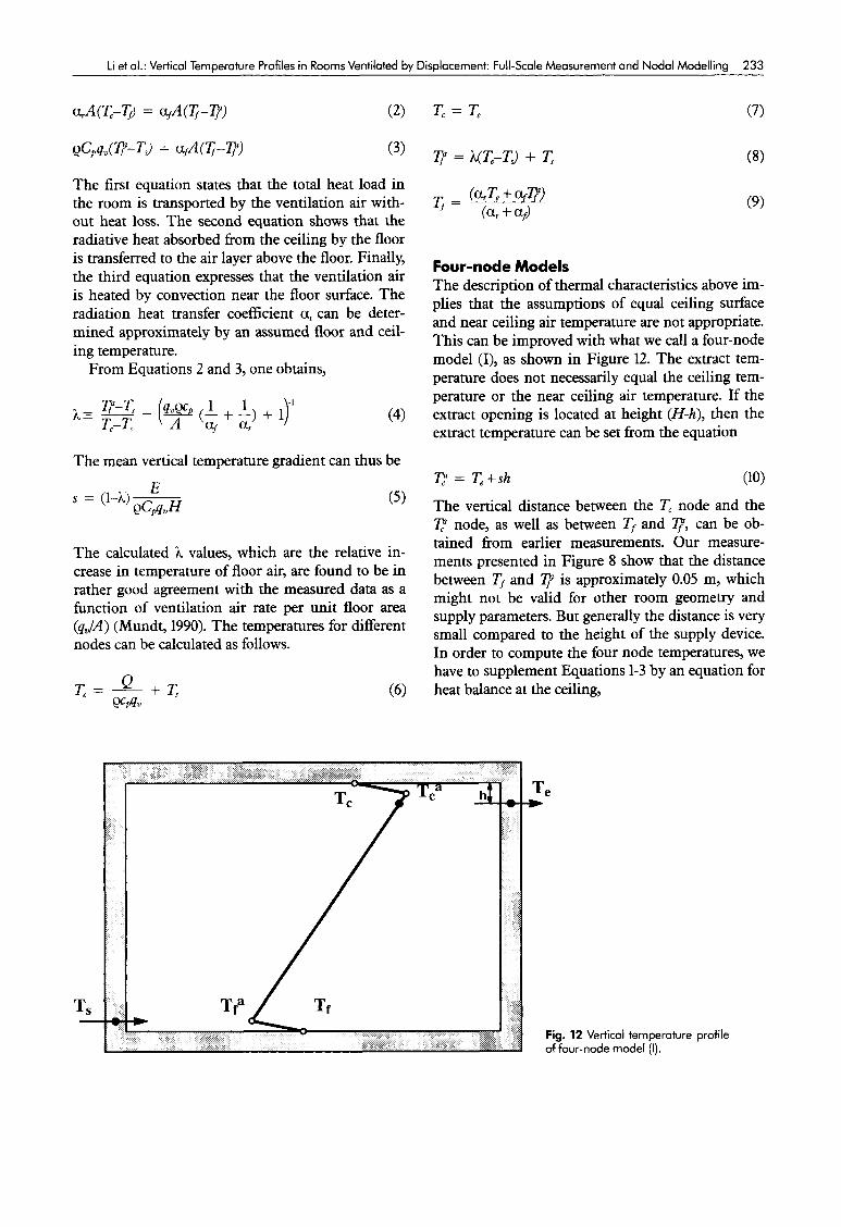
Four-node Models The description of thermal characteristics above im- plies that the assumptions of equal ceiling surface and near ceiling air temperature are not appropriate. This can be improved with what we call a four-node model (I), as shown in Figure 12. The extract temperature does not necessarily equal the ceiling temperature or the near ceiling air temperature. If the extract opening is located at height (H-h), then the extract temperature can be set from the equation

= T,+sh (10)

The vertical distance between the node and the Ip node, as well as between Tf and 7, can be obtained from earlier measurements. Our measurements presented in Figure 8 show that the distance between Tf and is approximately 0.05 my which might not be valid for other room geometry and supply parameters. But generally the distance is very small compared to the height of the supply device. In order to compute the four node temperatures, we have to supplement Equations 1-3 by an equation for heat balance at the ceiling,

e

Fig. 12 Vertical temperature of four-node model (I).

profile


The additional equation (11) represents the emitted heat fiom the ceiling balanced by the convective heat transfer near the ceiling surface. Again, the relative temperature ratio h and the temperature gradient s can be obtained.

-1 1 1 a, a, a,

h = (F (L + - + -) +1)

The only difference between Equations 12 and 4 is an extra term Va, in Equation 12. The temperature for different nodes can be calculated by

+ T , T , = - FPqv

L:

The four-node model (I) can be further modified to include the heat conduction through both the ceiling and the floor. In general, heat is gained at the lower part of the room and lost through the upper part of the room. Depending on the insulation and the indoor and outdoor thermal conditions, the heat load may be globally increased or decreased. When heat conduction is to be considered, the four-node model (11) in Figure 13 can be used. It is still called the four-node model because the outdoor temperature To is in general regarded as known. The three balance equations have to be modified. These are the heat balances at ceiling and floor surfaces (Equa- tions 19 and 20) as well as total room air (Equation 21).

a,A(c-TJ = a,A(K-T) + UcA(K-To) (19)

The explicit expressions for s and h are very complex, and a system of linear equations should be solved. Instead of using fmr-node model (II), we develop a multi-node model to include the various heat transfer modes. The four-node model used later refers to four-node model (I).

e

Fig. 13 Vertical temperature of four-node model (11).

profile


T O

Fig. 14 Vertical temperature T O of six-node model.

profile

Fig. 15 Vertical temperature profile T O of multi-node model.

Multi-node Model No heat transfer has been considered for the vertical walls. The upper parts of the walls “see” primarily the warm ceiling, while the lower parts “see” primarily the cold floor, so the wall temperature will vary with the height (Figure 8). Depending upon the outdoor temperature and wall insulation conditions, we may also have an outllow of heat through the upper part of the walls, and an inflow of heat through the lower part. A simple way to treat the vertical walls is to develop a six-node model as

shown in Figure 14. The total room air heat balance can be written as

A practical question is how to determine the border between the upper and lower parts of the vertical wall. A better solution has not been found except to determine it on the basis of experience from the

236 Li et 01.: Vertical Temperature Profiles in Rooms Ventilated by Displacement Full-Scale Measurement and Nodal Modelling

previously measured data. Another idea is to develop a multi-node model as shown in Figure 15. Each vertical wall surface is subdivided into Nk small surface elements. The height of an element is AH/Nk. A total of N = 4Nk + 2 sub-surface elements is obtained including the floor surface and the ceiling surface. For each surface, the heat balance equation can be established as

UALZ1-T) + acIAI~G-T) + (3 2 E , G , , ~ ; ~ A ~ - 0 ~ ~ T4A, = 0 1 = 1 (23)

N

The terms on the lefi-hand side represent the heat conduction through the wall, the convection, the absorbed radiation and emitted radiation, respectively. The Gebhart's absorption factor G, provides the fraction of energy emitted by a surface that is absorbed at another surface after reaching the absorb- ing surface by all possible paths. It can be obtained by the equation below for i = 1 to N andj = 1 to N .

N

GI] = a] + 2 Gk] @&k (24) k = l

The shape factor F, is calculated by the same method as in the two-band radiation model (Li and Fuchs, 1991). Even if we divide each vertical wall into 10 elements, the total number of elements is 42. This is different from the radiation model in other rooms, where the surface is divided in two direc- tions. The storage of shape factors in the multi-node model is thus reduced to an acceptable level by using the stratified feature. Two balance equations are available for the air in the gravity current and the air in the room, respectively. It may be noted here that unlike Equations 21 and 22 with conduction terms, Equation 26 uses the essentially equivalent convection term

Equation 25 can be used to determine the air temperature in the gravity current, T .

Equation 26 can be used to determine the temperature gradient in the room, which, in turn, gives the near ceiling air temperature Ip after obtaining p . If we separate the wall sub-surfaces into floor surface, ceiling surface and the sub-surfaces for four vertical walls, we can rewrite Equation 26 as,

where

Ip = F + s H

T, = V +s(H-h)

The formula for the temperature gradient can be calculated as

A B

s = -

where

A = E-Fpqv(F-lJ-afAf(F-p) 4 N A

i = l k = l

i = l k = l

The numerical calculation procedure is as follows:

give proper initial values for T,, p, 'Ip, and Te; obtain the approximate value of T, using Equation 23 with the Newton-Raphson method; obtain the approximate value using Equation 27; obtain the approximate value of the temperature gradients using Equation 29 as well as Ip and T,. repeat from the second step until the values of Ip and converge.

The calculation time for a typical case is around 30 seconds on an IBM RISC/6000-530 workstation, when each vertical wall is divided into eight elements. One precaution when using these models is the selection of the convective heat transfer coeG-

Li et 01.: Vertical Temperature Profiles in Rooms Ventilated by Displacement Full-Scale Measurement and Nodal Modellino 237

cients. The result obtained by the three-node model may be adjusted by using a smaller value of convective heat transfer coefficient to be equivalent to the result obtained by the four-node model with a larger value of convective heat transfer coefficient. This is due to the fact that the only difference between the three- and four-node models is that the four-node model also includes the convective component at the ceiling. Mundt (1990) used coefficient af of 3-5 W/mZoC and obtained good agreement between the model and the experiments. The coefficients af and a, used in our calculation here are within 5-7 W/ mz0C.

Results and Discussion Four-node Model The computed and measured results are compared in Figures 16-18 for different cases. In the cases presented in Figures 16 and 17, the heat carried by the ventilation air is approximately equal to the heat load in the room. This does not mean that the room walls are perfectly insulated, but rather that the heat loss in the upper part of the room equals the heat gain in the lower part. In this case, the deviation of the predicted near-floor and near-ceiling temperatures compared to the experimental result is less than 0.5 "C. Figure 17 shows a special case with aluminium walls; therefore, the emissivity in this case is set as 0.1. The results with an emissivity of 0.2 are also presented to show the sensitivity of the calculation at low emissivity. It can be seen that the four-

node model produces a better approximation than the three-node model. The assumption of a linear vertical profile does not agree with the measured profile. The reason for this is that in our experiments, a low cubic heat source is used. The upper part of the room exhibits a more pronounced mixing. In Figure 18, the heat loss through the wall is estimated to be about 10% of the heat load (450 W). This explains why we obtain a higher near-ceiling air temperature. In summary, the four-node model predicts well the magnitude of the temperature of air near the floor and ceiling and consequently the mean temperature gradient.

Figure 19 shows an example of the application of the four-node model. The effect of surface radiative properties is studied. It can be seen that lower emissivity walls result in higher stratification. These results agree well with the conclusions drawn from the measurements as shown in Figure 8. It is also found that at low levels of emissivity, the calculations are very sensitive to the emissivity.

Multi-node Model When the conduction heat loss is considerable, the multi-node model can be applied. This is evaluated for case B2 in Table 1. The results are shown in Fig- ure 20. Ignoring the heat loss in the four-node model leads to overprediction of the temperature and the temperature gradient. The predicted and measured heat losses are compared in Table 2. In the calculations, each vertical wall is divided into eight elements.

8 Temperature(T-Ts) ("C)

Fig. 16 Comparison between computed and measured vertical temperature profiles in rooms with black walls (case B3).

238 Li et 01.: Vertical Temperature Profiles in Rooms Ventilated by Displacement: Full-Scale Measurement and Nodal Modellina

Temperature(T-Ts) ("C)

2.5

2.0

n E y 1.5

.3 5 3

1 .o

0.5

0 2 4 6 8 Temperature(T-Ts) ("C)

The rather good agreement gives us confidence when using the multi-node model to study the effects of heat conduction on the temperature profile. We chose a standard room with structures the same as the test room. The standard conditions are To = 21 "C, E = 300 W, = 19 "C and n = 3. The calculations are made by changing one parameter each time. The vertical air temperature profiles are presented in Figure 21, with the corresponding heat losses in Figure 22. In Figure 22b, the case number R corresponds to 100-R watts heat load in the room. In general, we can conclude that the higher the supply

10 12

Fig. 17 Comparison between computed and measured vertical temperature profiles in rooms with aluminium walls (case A2).

Fig. 18 Comparison between computed and measured vertical temperature profiles in rooms with black walls (case 84).

temperatures and heat loads and the lower the outdoor temperatures and supply flow rates, the higher the heat loss. For this badly-insulated room, when the outdoor temperature is very low (5 "C), the heat load is completely lost in a global sense. The results

Table 2 Comparison between predicted and measured heat losses

Case No. Measured Qmr (W) Predicted Q- (W)

B1 171. 190. B2 224. 230.

Li et al.: Vertical Temperature Profiles in Rooms Ventilated by Displacement: Full-Scale Measurement and Nodal Modelling 239

indicate that the floor surface temperature and vertical temperature gradient are a function of heat conduction, convection and radiation.

0 The vertical temperature profile is affected con- siderably by conduction through the wall and the radiative heat transfer between room surfaces, particularly between the ceiling and the floor.

Concluding Remarks 0 Different heights of heat source lead to different

temperature profiles, but the stationary front re- In the present paper, the vertical temperature pro- mains unchanged. files in rooms ventilated by displacement have been 0 The simple four-node model (I) predicts the investigated experimentally and by approximate mean vertical temperature gradient in the room models. The following conclusions have been well, when the heat loss is not significant com- drawn:

2.5

2.0

- E E - 1.5

M .+

1.0

0.5

pared to the heat load in the room (< 10%). The multi-

- emissiviry=O.I -..-.. emissiviry=0.3

0 eniissivity=O.S . . - emissivity=0.7

0 -- emissivity=0.9 0 emissivily=l.O

Fig. 19 Predicted temperature profiles with different wall surface emissivities

heat load). Temperature(T-Ts) ("C)

0.0 (3 room volumes/hour and 300 W 0 1 2 3 4 5

2.5 0 - Airjmeasured) 0 - Wall(measured)

P . .. Wall(mul1i-node model) ---- Air(four-node model)

..... Air(rnulti-node model)

I

n

E E - 1.5

bD .*

si 1.0

0.5

,d- -___ _ _ - ,

walls (case 82) Temperature(T-Ts) ("C) 0 2 4 6 8 1 0 12

Fig. 20 Comparison between computed and measured vertical temperature profiles in roams with black

0.0


N

* O 1 <

m

P

W

G In

Fig. 21 Predicted temperature profiles with (a) different outdoor temperatures; (b) different heat loads; (c) different supply temperatures; (d) different supply flow rates.


.I Y

0 a

h

W a

b n e i

a 1 0 > I

0

U U n

3 W

u

Fig. 22 Predicted heat losses with (a) different outdoor temperatures; (b) different heat loads (case number k corresponds to 100 . k watts heat load); (c) different supply temperatures; (d) different supply flow rates.


node model also shows a rather good agreement between the models and the experiment, when the heat loss is larger ( > 10%).

0 The simplified nodal models have left out entirely the turbulent transport in the room. A possible extension of the models could be achieved by coupling them to the two-zone model to consider the mixing process in the upper polluted zone.

0 The models developed can be used for thermal comfort analysis and energy consumption analysis which are mostly based on a uniform indoor air temperature. The model can also supply the thermal boundary conditions for CFD codes.

Acknowledgements The authors would like to thank Elisabeth Linden for her help with the smoke tests and Dr. Sture Holmberg and Tech. Lic. Elisabeth Mundt for their interest and discussions. During the course of the measurements, the first author worked at the Nat- ional Swedish Institute for Building Research. This work was financially supported by the Swedish Council for Building Research (BFR).

Nomenclature A =

Ar = B = cp = E = F =

h =

H = n = N = Nk =

4 n =

G.. = 11

QWIF s = T = T . =

OSI

u = u = us =

aluminium wall case (in Table 1); floor and wall surface area (m2) Archimdes number g(ATdTo)HdUs black wall case (in Table 1) specific heat of air (J/KgK) heat load in the room (W) shape factor Gebhart’s absorption factor distance between ceiling and extract opening centre (m) room height (m) specific flow rate (room volume/hour) total number of sub-surfaces number of sub-divisions of the vertical walls supply flow rate (m3/s) heat removed by ventilation air (W) temperature gradient dT/dH (K/m) temperature (“C) exterior surface temperature of wall No. i in Table 1 (“C) velocity (m/s) conductive heat transfer coefficient (U-value) (W/m2K) supply velocity (m/s)

Greek Symbols a = a , = AH= AT,= E =

A = P = o =

convective heat transfer coefficient (W/m2K) radiative heat transfer coefficient (W/m2K) height of the sub-surface of the vertical walls reference temperature difference (K) emissivity

air density (Kg/m3), reflectivity Stefan-Boltzman constant (5.6697 x W/ m2K4)

ratio of T-Ts to Te-Ts.

Subscripts c = ceiling e = extract f = floor o = outdoor s = supply w = wall 0 = reference quantity

superscripts a = indoor air L = lowerpartofthewall U = upperpartofthewall

References Beier, R.A. and Gorton, R.L. (1978) “Thermal stratification in

factories - cooling loads and temperature profiles”, ASHRAE Eansmtwns, 84, Pt. 1,325-338.

Chen, Q. and van der Kooi, J. (1990) “A methodology for indoor airflow computations and energy analysis for a displacement ventilation system”, Energy and Buildings, 14,259-271.

Davidson, L. (1989) “Ventilation by displacement in a three-dimensional room: a numerical study”, Building and Environ-

Heiselberg, I? and Sandberg, M. (1990) “Convective from a slender cylinder in a ventilated room”. In: Froceedings of Roomvent ’90, Oslo, Norway, June 13-15.

Howarth, A.T. (1983) Temperature Distributwn and Air Movements in Rooms with Convective Heat Source, Ph.D. thesis, University of Manchester, Institute of Science and Technology, UK.

Inard, C. and Buty, D. (1991) “Simulation of thermal coupling between a radiator and a room with zonal models”. In: Clarke, J.A., Mitchell, J.W. and Van de Perre, R.C. (eds), Proceedings of Building Simulation 91, Nice, France, August, 20-22. pp. ll347.

Johansson, A.V. and Alfredsson, EH. (1982) “On the structure of turbulent channel flow”, Jounzal of Fluid Mechanics, 122, 295- 314.

Li, Y. and Fuchs, L. (1991) “A two-band radiation model for cal- culating room wall surface temperature”. In: Sunden, B. and Zukauskas, A. (eds), Recent Advances in Heat Transfm, Elsevier Science Publishers, pp. 388-400.

Li, Y., Sandberg, M. and Fuchs, L. (1992) “Radiative effects on airflow with displacement ventilation: An experimental invest- igation”. To be published in Energy and Buildings.

Mathisen, H.M. (1990) “Displacement ventilation-the influence of the characteristics of the supply air terminal device on the airflow pattern”, Indoor Air, sample issue, 0 (0), 3-20.

Mundt, E. (1990) “Convection flows above common heat sources

M t , 24 (4), 363-372.


in room with displacement ventilation”. In: Proceedings of h v e n t ’ 9 0 , Oslo, Norway, June 13-15.

Mundt, E. (1991) Temperature Gradients and Convection Flows with Dispkement Ventilation, Tech. Lic. Thesis, Department of Building Services Engineering, Royal Institute of Technology, Stockholm, Sweden.

Nielsen, EV., Hoff, L. and Pedersen, L.G. (1988) “Displacement ventilation by different types of diffusers”. In: Proceedings of 9th AZVC Confuence, Gent, Belgium, 12-15 September.

Overby, H. and Steen-Thode, M. (1990) “Calculation of vertical temperature gradients in heated rooms”. In: Proceedings of Roomvent 90, Oslo, Norway, June 13-15.

Sandberg, M. (1985) Lujiutbyteseffektivitet Vatikztionseffektivitet Temperacur- Effektivitet i Cellkontot, Gavle, Sweden, Swedish In- stitute for Building Research, (Meddelande M85:24).

Sandberg, M. and Lindstrom, S. (1987) “A model for ventilation by displacement”. In: Proceedings of Roomvent ’87, Stockholm, Sweden, 10-12 June.

Sandberg, M. and Blomqvist, C. (1989) “Displacement ventilation in office rooms”. Paper presented at ASHRAE Confuence, Van- couver, Canada, 25-28 June.

Sandberg, M. and Lindsuom, S. (1990) “Stratified flow in ventilated rooms-A model study”. In: Proceedings of Roomvent ’90, Oslo, Norway, June 13-15.

Sandberg, M. and Mattsson, M. (1991a) “The mechanism of spread of negatively buoyant air flow low velocity air terminals’’. Paper presented at ZV Seminar on Application of Fluid Mechanics in Environment Protection ’91, Wisla, Polen, 22-24 April.

Sandberg, M. and Mattsson, M. (1991b) “Two-dimensional non- isothermal supply flom low velocity terminals”, Air Znfiltraria

Wyon, D.l? and Sandberg, M. (1990) “Thermal manikin prediction of discomfort due to displacement ventilation”, ASHRAE

R&, U (2), 12-14.

TransactWn~, %, Pt. 1,67-75.

Vertical Temperature Profiles in Rooms Ventilated by Displacement: Full-Scale Measurement and Nodal...

Documents

Transcript of Vertical Temperature Profiles in Rooms Ventilated by Displacement: Full-Scale Measurement and Nodal...