venkateshwara - open university
226
VENKATESHWARA OPEN UNIVERSITY www.vou.ac.in BUSINESS ECONOMICS BBA [BBA-101]
-
Upload
khangminh22 -
Category
Documents
-
view
0 -
download
0
Transcript of venkateshwara - open university
BUSINESS ECONOMICS
VENKATESHWARAOPEN UNIVERSITY
www.vou.ac.in
VENKATESHWARAOPEN UNIVERSITY
www.vou.ac.in
BUSINESS ECONOMICS
BUSINESS ECONOMICS
10 MM
BBA[BBA-101]

BUSINESS ECONOMICS
BBA
[BBA-101]
Copyright © D N Dwivedi, 2019
BOARD OF STUDIES
Prof Lalit Kumar SagarVice Chancellor
Dr. S. Raman IyerDirectorDirectorate of Distance Education
SUBJECT EXPERT
Dr. S. Raman IyerDr. Richa AgarwalDr. Anand KumarDr. Babar Ali KhanDr. Adil Hakeem Khan
Programme DirectorAssistant ProfessorAssistant ProfessorProfessor in CommerceProfessor in Management
CO-ORDINATOR
Mr. Tauha KhanRegistrar
All rights reserved. No part of this publication which is material protected by this copyright noticemay be reproduced or transmitted or utilized or stored in any form or by any means now known orhereinafter invented, electronic, digital or mechanical, including photocopying, scanning, recordingor by any information storage or retrieval system, without prior written permission from the Publisher.
Information contained in this book has been published by VIKAS® Publishing House Pvt. Ltd. and hasbeen obtained by its Authors from sources believed to be reliable and are correct to the best of theirknowledge. However, the Publisher and its Authors shall in no event be liable for any errors, omissionsor damages arising out of use of this information and specifically disclaim any implied warranties ormerchantability or fitness for any particular use.
Vikas® is the registered trademark of Vikas® Publishing House Pvt. Ltd.
VIKAS® PUBLISHING HOUSE PVT LTDE-28, Sector-8, Noida - 201301 (UP)Phone: 0120-4078900 Fax: 0120-4078999Regd. Office: A-27, 2nd Floor, Mohan Co-operative Industrial Estate, New Delhi 1100 44Website: www.vikaspublishing.com Email: [email protected]

Concept:Meaning, Nature, Scope and Significance of Business Economic
Utility Approach:Law of Diminishing Marginal Utility, Law of Utility
Demand Analysis and Forecasting:Demand Schedule and Demand Curve, Significance of DemandForecasting and Techniques.
Production Function:Concept, Break Even analysis, Law of Variable Proportion.
Cost… Revenue:Concept, Short Run and Long Run Cost Curves, Concept of Total,Marginal and Average Revenues, Relationships between AverageRevenue, Marginal Revenues and Elasticity of Demand.
Pricing:Objectives of the Firm - Profit Maximization/Sales RevenueMaximization Survival, Pricing under Different Market Structures -Perfect Competition, Monopoly, Discriminating, Product - LinePricing, Joint Product Pricing.
Profit Management:Concept of Profit Management, Profit Planning and Control.
Unit 1: Introduction toBusiness Economics
(Pages: 3-26)
Unit 2: Utility Approach(Pages: 27-61)
Unit 3: Demand Analysis andForecasting
(Pages: 63-96)
Unit 4: Production Function(Pages: 97-128)
Unit 5: Cost and Revenue(Pages: 129-165)
Unit 6: Pricing(Pages: 167-197)
Unit 7: Profit Management(Pages: 199-213)
SYLLABI-BOOK MAPPING TABLEBusiness Economics
Syllabi Mapping in Book


CONTENTSINTRODUCTION 1
UNIT 1 INTRODUCTION TO BUSINESS ECONOMICS 3-261.0 Introduction1.1 Unit Objectives1.2 Understanding Economics and its Scope
1.2.1 Meaning and Nature of Business Economics1.2.2 Scope of Business or Managerial Economics1.2.3 Difference between Business or Managerial Economics and Pure Economics
1.3 Significance of business Decision-Making1.3.1 Managerial Economics: Techniques and Business Decisions1.3.2 Time Perspective in Business Decisions
1.4 Role of a Managerial Economist1.5 Summary1.6 Key Terms1.7 Answers to ‘Check Your Progress’1.8 Questions and Exercises1.9 Further Reading
UNIT 2 UTILITY APPROACH 27-612.0 Introduction2.1 Unit Objectives2.2 Law of Utility2.3 Law of Diminishing Marginal Utility
2.3.1 Analysis of Consumer Behaviour: Cardinal Utility Approach2.3.2 Analysis of Consumer Behaviour: Ordinal Utility Approach2.3.3 Meaning and Nature of Indifference Curve2.3.4 Consumer’s Equilibrium: Ordinal Utility Approach2.3.5 Derivation of Individual Demand Curve2.3.6 Comparison of Cardinal and Ordinal Utility Approaches
2.4 Summary2.5 Key Terms2.6 Answers to ‘Check Your Progress’2.7 Questions and Exercises2.8 Further Reading/Endnotes
UNIT 3 DEMAND ANALYSIS AND FORECASTING 63-963.0 Introduction3.1 Unit Objectives3.2 Demand Schedule and Demand Curve3.3 Significance of Demand Forecasting and Techniques
3.3.1 Steps in Demand Forecasting3.3.2 Techniques of Demand Forecasting
3.4 Some Case Studies of Demand Forecasting3.5 Summary3.6 Key Terms3.7 Answers to ‘Check Your Progress’3.8 Questions and Exercises3.9 Further Reading/Endnotes
UNIT 4 PRODUCTION FUNCTION 97-1284.0 Introduction4.1 Unit Objectives4.2 Production Function: Concept4.3 Break-even Analysis
4.3.1 Contribution Analysis4.3.2 Profit—Volume Ratio4.3.3 Margin of Safety
4.4 Law of Variable Proportion4.4.1 Determining Optimum Employment of Labour4.4.2 Isoquant Curves and their Properties4.4.3 Isoquant Map and Economic Region of Production4.4.4 Elasticity of Factor Substitution4.4.5 Laws of Returns to Scale
4.5 Summary4.6 Key Terms4.7 Answers to ‘Check Your Progress’4.8 Questions and Exercises4.9 Further Reading/Endnotes
UNIT 5 COST AND REVENUE 129-1655.0 Introduction5.1 Unit Objectives5.2 Cost Concepts5.3 Short and Long-Run Cost Curves
5.3.1 Cost Curves and the Law of Diminishing Returns5.4 Total, Marginal and Average Revenues
5.4.1 Price Elasticity of Demand5.4.2 Measuring Price Elasticity from a Demand Function5.4.3 Price Elasticity and Total Revenue5.4.4 Price Elasticity and Marginal Revenue5.4.5 Determinants of Price Elasticity of Demand5.4.6 Cross-Elasticity of Demand5.4.7 Income-Elasticity of Demand5.4.8 Advertisement or Promotional Elasticity of Sales5.4.9 Elasticity of Price Expectations
5.5 Summary5.6 Key Terms5.7 Answers to ‘Check Your Progress’5.8 Questions and Exercises5.9 Further Reading/Endnotes
UNIT 6 PRICING 167-1976.0 Introduction6.1 Unit Objectives6.2 Objectives of the Firm
6.2.1 Profit Maximization6.2.2 Sales Revenue Maximization
6.3 Pricing Under Different Market Structures6.3.1 Perfect Competion6.3.2 Monopoly6.3.3 Price Discrimination Under Monopoly6.3.4 Price Discrimination by Degrees

6.4 Product Line Pricing6.4.1 Joint Product Pricing
6.5 Summary6.6 Key Terms6.7 Answers to ‘Check Your Progress’6.8 Questions and Exercises6.9 Further Reading/Endnotes
UNIT 7 PROFIT MANAGEMENT 199-2137.0 Introduction7.1 Unit Objectives7.2 Concept of Profit Management
7.2.1 Monopoly Power as Source of Profit7.2.2 Problems in Profit Measurement7.2.3 Problem in Measuring Depreciation7.2.4 Treatment of Capital Gains and Losses7.2.5 Current vs Historical Costs
7.3 Profit Planning and Control7.3.1 Profit as Control Measure
7.4 Summary7.5 Key Terms7.6 Answers to ‘Check Your Progress’7.7 Questions and Exercises7.8 Further Reading/Endnotes

Self-InstructionalMaterial 1
Introduction
NOTES
INTRODUCTIONThe natural curiosity of a student, who begins to study a subject, is to know its natureand scope. Such as it is, a student of economics would like to know ‘what is economics’and ‘what is its subject matter’. Surprisingly, there is no precise answer to these questions.
Attempts made by economists over the past 300 years to define economics havenot yielded a precise and universally acceptable definition of economics. Economistsright from Adam Smith—the ‘father of economics’—down to modern economists havedefined economics differently, depending on their own perception of the subject matterof economics of their era. Thus, economics is fundamentally the study of choice-makingbehaviour of the people. The choice-making behaviour of the people is studied in asystematic or scientific manner. This gives economics the status of a social science.However, the scope of economics, as it is known today, has expanded vastly in the post-World War II period. Modern economics is now divided into two major branches:Microeconomics and Macroeconomics. Microeconomics is concerned with themicroscopic study of the various elements of the economic system and not with thesystem as a whole.
As economist Abba P. Lerner has put it, ‘Microeconomics consists of looking atthe economy through a microscope, as it were, to see how the millions of cells in bodyeconomic—the individuals or households as consumers and the individuals or firms asproducers—play their part in the working of the whole economic organism.’Macroeconomics is a relatively new branch of economics. Macroeconomics is the studyof the nature, relationship and behaviour of aggregates and averages of economicvariables. Therefore, the technique and process of business decision-making has of latechanged tremendously.
The basic functions of business managers is to take appropriate decisions onbusiness matters, to manage and organize resources, and to make optimum use of availableresources with the objective of achieving the business goals. In today’s world, businessdecision-making has become an extremely complex task due to the ever-growingcomplexity of the business world and the business environment. It is in this context thatmodern economics—howsoever defined—contributes a great deal towards businessdecision-making and performance of managerial duties and responsibilities. Just as biologycontributes to the medical profession and physics to engineering, economics contributesto the managerial profession.
The book has been written in keeping with the self-instructional mode or the SIM(self instructional material) format for distance learning. Each unit begins with anIntroduction to the topic, followed by an outline of the Unit Objectives. The detailedcontent is then presented in a simple and organized manner, interspersed with ‘CheckYour Progress’ questions to test the student’s understanding of the topics covered. ASummary along with a list of Key Terms and a set of Questions and Exercises isprovided at the end of each unit for effective recapitulation.

Self-InstructionalMaterial 3
Introduction to BusinessEconomics
NOTES
UNIT 1 INTRODUCTION TOBUSINESS ECONOMICS
Structure1.0 Introduction1.1 Unit Objectives1.2 Understanding Economics and its Scope
1.2.1 Meaning and Nature of Business Economics1.2.2 Scope of Business or Managerial Economics1.2.3 Difference between Business or Managerial Economics and Pure Economics
1.3 Significance of business Decision-Making1.3.1 Managerial Economics: Techniques and Business Decisions1.3.2 Time Perspective in Business Decisions
1.4 Role of a Managerial Economist1.5 Summary1.6 Key Terms1.7 Answers to ‘Check Your Progress’1.8 Questions and Exercises1.9 Further Reading
1.0 INTRODUCTION
Emergence of business or managerial economics as a separate course of managementstudies can be attributed to at least three factors: (a) growing complexity of the businessdecision-making process due to changing market conditions and business environment,(b) consequent upon, the increasing use of economic logic, concepts, theories andtools of economic analysis in the process of business decision-making, and (c) rapidincrease in demand for professionally trained managerial manpower. Let us have aglance at how these factors have contributed to the creation of ‘managerial economics’as a separate branch of study.
It is a widely accepted fact that the business decision-making process has becomeincreasingly complicated due to ever growing complexities in the business world.There was a time when business units (shops, firms, factories, mills) were set up,owned and managed by individuals or business families. In India, there were 22 topbusiness families like the Tatas, Birlas, Singhanias, Ambanis and Premjis. Big industrieswere few and the scale of business operation was relatively small. The managerialskills acquired through traditional family training and experience were sufficient tomanage small and medium scale businesses. Although a large part of private businessis still run on a small scale and managed in the traditional style of business management,the industrial business world has changed drastically in size, nature and content. Thegrowing complexity of the business world can be attributed to the growth of largescale industries, growth of a large variety of industries, diversification of industrialproducts, expansion and diversification of business activities of corporate firms, growthof multinational corporations, and mergers and takeovers, especially after the SecondWorld War. These factors have contributed a great deal to the recent increase in inter-firm, inter-industry and international rivalry, competition, risk and uncertainty. Business
Self-Instructional4 Material
Introduction to BusinessEconomics
NOTES
decision-making in this kind of business environment is a very complex affair. The familytraining and experience is no longer sufficient to meet the managerial challenges.
The growing complexity of business decision-making has inevitably increased theapplication of economic concepts, theories and tools of economic analysis in this area.The reason is that making an appropriate business decision requires a clear understandingof market conditions, the nature and degree of competition, market fundamentals andthe business environment. This requires an intensive and extensive analysis of the marketconditions in the product market, input market and financial market. On the other hand,economic theories, logic and tools of analysis have been developed to analyse and predictmarket behaviour. The application of economic concepts, theories, logic and analyticaltools in the assessment and prediction of market conditions and business environmenthas proved to be of great help in business decision-making. The contribution of economicsto business decision-making has come to be widely recognized. Consequently, economictheories and analytical tools, which are widely used in business decision-making havecrystallized into a separate branch of management studies, called managerial economicsor business economics.
1.1 UNIT OBJECTIVES
After going through this unit, you will be able to:• Discuss the concept of economics and its scope• Explain the nature and scope of business economics• Discuss the significance of business decision-making• Discuss the role and responsibility of a managerial economist in a business
enterprise
1.2 UNDERSTANDING ECONOMICS AND ITSSCOPE
Let us begin our study of business or managerial economics by learning• What is economics?• What are business or managerial decision-making problems?• How does economics contribute to business decision-making?
What is Economics?
The natural curiosity of a student who begins to study a subject is to know the natureand scope of the subject of his study. Such as it is, a student of economics would liketo know ‘What is economics’ and ‘What is its subject matter’. Surprisingly, there isno precise answer to these questions. Attempts made by economists over the past 300years to define economics have not yielded a precise and universally acceptabledefinition of economics. Economists right from Adam Smith—the ‘father ofeconomics’—down to modern economists have defined economics differently,depending on their own perception of the subject of their era. For example, AdamSmith (1776) defined economics as ‘an inquiry into the nature and causes of thewealth of the nations’. Nearly one-and-half centuries later, Alfred Marshall, an all-time
Self-InstructionalMaterial 5
Introduction to BusinessEconomics
NOTES
great economist, defined economics differently. According to Alfred Marshall (1922),‘Economics is the study of mankind in the ordinary business of life; it examines that partof individual and social action which is most closely connected with the attainment andwith the use of the material requisites of well being.’ Lionel Robbins (1932) has definedit more precisely: ‘Economics is the science which studies human behaviour as arelationship between ends and scarce means which have alternative uses.’ One can finda number of other definitions in various writings on economics. None of these definitionshowever, capture the entire subject matter of modern economics, although each throwssome light on what economics is about.
The fact is that economics has not yet been defined precisely and appropriately.The reason is, as Zeuthen has observed, ‘Economics is an unfinished science’ and asSchultz has remarked, ‘Economics is still a very young science and many problems init are almost untouched.’ These observations, made half a century ago, still hold true.It seems that after Robbins, no serious attempt was made to define economics. Definingeconomics has been such a fruitless endeavour that some modern authors of economicstexts, including those by reputed economists like Samuelson, Baumol and Stiglitz,avoid the issue of defining economics. For example, William J. Baumol (a Nobellaureate) and Allen S. Blinder write in their own text, ‘Many definitions of economicshave been proposed, but we prefer to avoid any attempt to define the discipline in asingle sentence or paragraph’, and let ‘the subject matter speak for itself.’
However, the study of economic science, or of any science for that matter,must commence with a working definition of it. In this regard, most modern textsfollow Robbins’ definition of economics, even though modern economics goes farbeyond what Robbins thought the subject matter of economics was. Let us begin bylooking at Robbins’ view and then study how far economics goes beyond his view.
Economics is a Social Science
Economics as a social science studies economic behaviour of the people and itsconsequences. What is economic behaviour? Economic behaviour is essentially theprocess of evaluating economic opportunities open to an individual or a society and,given the resources, making a choice of the best of these opportunities. The objectivebehind this is to maximize gains from the available resources and opportunities. Intheir efforts to maximize gains from their resources, people have to make a numberof choices regarding the use of resources and spending their earnings.
The basic function of economics is to observe, explain and predict how people(individuals, households, firms and the government) as decision-makers make choicesabout the use of resources (land, labour, capital, knowledge and skills, technology,time and space, etc.) in order to maximize their income, as well as how they, asconsumers, decide how to spend their income to maximize their total utility. Thus,economics is fundamentally the study of choice-making behaviour of the people.Studying it in a systematic or scientific manner gives economics the status of a socialscience.
For the purpose of economic analysis, people are classified according to theirdecision-making capacity as individuals, households, firms and the society; andaccording to the nature of their economic activity as consumers, producers, factoryowners and economy managers, i.e., the government. As consumers, individuals andhouseholds, with a given income they have to decide ‘what to consume and howmuch to consume’. They have to make these decisions because consumers are, by
Self-Instructional6 Material
Introduction to BusinessEconomics
NOTES
nature, utility maximizers, and consuming any commodity in any quantity does notmaximize their gains or their satisfaction. As producers, firms, farms, factories,shopkeepers, banks, transporters, etc., they have to choose ‘what to produce, how muchto produce and how to produce’, because they too are gain maximizers and producingany commodity in any quantity by any technique will not maximize their gains (profits).As labour, they have to choose between alternative occupations and places of workbecause any occupation at any place will not maximize their earnings. Likewise, thegovernment has to choose how to tax, whom to tax, how much to spend and how tospend, so that social welfare is maximized at a given social cost. Economics as a socialscience studies how people make their choices.
It is this economic behaviour of the individuals, households, firms, governmentand the society as a whole which forms the central theme of economics as a socialscience. Thus, economics is fundamentally the study of how people allocate theirlimited resources to produce and consume goods and services to satisfy their endlesswants, with the objective of maximizing their gains.
Why does the problem of making choices arise?
The need for making choice arises because of some basic facts of economic life. Letus look at the basic facts of human life in some detail and how they create the problemof choice-making.
(i) Human wants, desires and aspirations are limitless: The history of humancivilization bears evidence to the fact that human desire to consume more andmore of better and better goods and services has always been increasing. Forexample, the housing need has risen from a hut to a luxury palace, and if possible,a house in space; the need for means of transportation has gone up from mulesand camels to supersonic jet planes; demand for means of communication hasrisen from messengers and postal services to cell phones with cameras; needfor computational facility from manual calculation to superfast computers, andso on. For an individual, only the end of life brings an end to his/her needs.
Human wants, desires and needs are endless in the sense that they go onincreasing with increase in people’s ability to satisfy them. The endlessness ofhuman wants can be attributed to (i) people’s insatiable desire to raise theirstandard of living, comforts and efficiency, (ii) human tendency to accumulatethings beyond their present need, (iii) increase in knowledge about inventionsand innovations of new goods and services with greater convenience, efficiencyand serviceability, (iv) multiplicative nature of some want (e.g., buying a carcreates want for many other things—petrol, driver, cleaning, parking place,safety locks, spare parts, insurance), (v) biological needs (e.g., food, water)are repetitive, (vi) imitative and competitive nature of needs of human beingsdue to demonstration and bandwagon effects, and (vii) influence ofadvertisements in modern times creating new kinds of wants. For these reasons,human wants continue to increase endlessly.
Apart from being unlimited, another and an equally important feature ofhuman wants is that they are gradable. In simple words, all human wants are notequally urgent and pressing at a point of time, or over a period of time. Whilesome wants have to be satisfied as and when they arise (e.g., food, clothes andshelter), some can be postponed (e.g., purchase of a car). Also, satisfyingsome wants provides greater satisfaction than others. Given their intensity and

Self-InstructionalMaterial 7
Introduction to BusinessEconomics
NOTES
urgency, human wants can be arranged in the order of their priority. The priorityof wants, however, varies from person to person, and from time to time for thesame person. Therefore the question arises as to ‘which want to satisfy first’ and‘which the last’. Thus, consumers have to make a choice between ‘what toconsume’ and ‘how much to consume’. Economics studies how consumers(individuals and household) make choices between their wants and how theyallocate their expenditure between the different kinds of goods and servicesthey choose to consume.
(ii) Resources are scarce: The need for making a choice between the variousgoods that people want to produce and consume arises mainly because theresources that are available to the people at any point of time for satisfying theirwants are scarce and limited. What are these resources? Conceptually, anythingwhich is available and can be used to satisfy human wants and desires is aresource. In economics, however, the resources that are available to individuals,households, firms, and societies at any point of time are traditionally classifiedas follows:• Natural resources (including cultivable land surface, space, lakes, rivers,
coastal range, minerals, wildlife, forest, climate, rainfall, etc.).• Human resources (including manpower, human energy, talent, professional
skill, innovative ability and organizational skill, jointly called labour).• Man-made resources (including machinery, equipments, tools, technology
and building, called together capital).• Entrepreneurship, i.e., the ability, knowledge and talent to put land, labour
and capital in the process of production, and the ability and willingness toassume risk in business.
To these basic resources, economists add other categories of resources, viz.,time, technology and information. All these resources are scarce. Resourcescarcity is a relative term. It implies that resources are scarce in relation to thedemand for resources. The scarcity of resources is the mother of all economicproblems. If resources were unlimited, like human wants, there would be noeconomic problem and, perhaps, no economics as a subject of study. It is thescarcity of resources in relation to human wants that forces people to makechoices.
Furthermore, the problem of making choices arises also because resourceshave alternative uses and these alternative uses have different returns or earnings.For example, a building can be used to set up a shopping centre, businessoffice, a public school, a hospital or for residential purposes. But the return onthe building varies according to the use of the building. Therefore, a return-maximizing building owner has to make a choice between the alternative uses ofthe building. If the building is put to a particular use, the landlord has to foregothe return expected from its other alternative uses. This is called opportunitycost. Economics as a social science analyses how people (individuals andsociety) make choices between the economic goals they want to achieve, betweenthe goods and services they want to produce, and between the alternative usesof their resources with the objective of maximizing their gains. The gain-maximizers evaluate the costs and benefits of the alternatives while deciding onthe final use of the resources. Economics studies the process of making choicesbetween the alternative uses. According to Robbins, this is what constitutes thesubject matter of economics.
Self-Instructional8 Material
Introduction to BusinessEconomics
NOTES
(iii) People are gain maximizers: Yet another important aspect of human naturethat leads to choice-making behaviour is that most people aim at maximizing theirgains from the use of their limited resources. ‘Why people want to maximize theirgains’ is a no concern in economics. Traditional economics assumes maximizingbehaviour of the people as a part of their rational economic behaviour. Thisassumption is based on observed facts. As consumers, they want to maximizetheir utility or satisfaction; as producers, they want to maximize their output orprofit; and as factor owners, they want to maximize their earnings. People’sdesire to maximize their gains is a very important aspect of economic behaviourof the people giving rise to the need to study economics. If people did not want tomaximize their gains, the problem of choice-making would not arise. Consumerswould not bother as to ‘what to consume’ and ‘how much to consume’; producerswould not bother as to ‘what to produce’, ‘how much to produce’ and ‘how toproduce’; and factor owners would not care as to where and how to use theresources. But, in reality, they do maximize their gains and economics studieshow people maximize their gains.
Economics goes far beyond choice-making behaviour
The foregoing description of economics may give the impression that economics endswith the study of choice-making behaviour of the people but it is not quite so. Economicsgoes far beyond the scope of microeconomics. If economics is confined to the study ofchoice-making behaviour of the individual, many other and more important economicissues that constitute a major part of modern economic science will have to be left out.Look at some of the major national and international, economic issues:
• How is the level of national output and employment determined in a country?• Why are some countries very rich and some countries very poor?• What are the factors that determine the overall economic growth of a country?• What causes fluctuations in the national output, employment and the general price
level?• How do international trade and international capital flows affect the domestic
economy?• What causes inflation and what are its effects on the economy’s growth and
employment?• Why is about 35 per cent of India’s population still ‘below the poverty line’
even after five decades of planned development with emphasis on ‘removal ofpoverty’?
• Why is there large-scale unemployment in India and why have the efforts tosolve the problem of unemployment failed?
• Why has the Government of India been faced with fiscal deficits of a dangerousmagnitude over the past two decades and why has it failed to reduce it to amanageable level?
• Why does the government need to intervene with the market system and adoptmeasures to control and regulate production and consumption, saving andinvestment, export and imports, wages and prices, and so on?One can point out many other issues which do not fall within the purview of
microeconomics. Analysis of and finding answers to such economic problems now

Self-InstructionalMaterial 9
Introduction to BusinessEconomics
NOTES
constitute a major and a more important subject matter of economics than the choice-making aspect of it. The study of the issues mentioned above has created a relativelynew branch of economics, called macroeconomics. As noted above, the field ofeconomics continues to grow and expand in its scope, size and analytical rigour.Boundaries of economic science are not yet precisely marked, though economics isclaimed to be ‘the oldest and best developed of the social sciences’. Let us nowglance at the scope of economics as it is known today, and the major branches andspecialized areas of economics.
Scope of Economics
As noted earlier, the scope of economics is not marked precisely and, as it appears, itcannot be. However, the scope of economics, as it is known today, has expandedvastly in the post-World War II period. Modern economics is now divided into twomajor branches: microeconomics and macroeconomics. A brief description of thesubject matter and approach of microeconomics and macroeconomics is given below.
Microeconomics
Microeconomics is concerned with the microscopic study of the various elements ofthe economic system and not with the system as a whole. As Lerner has put it,‘Microeconomics consists of looking at the economy through a microscope, as itwere, to see how the million of cells in body economic—the individuals or householdsas consumers and the individuals or firms as producers—play their part in the workingof the whole economic organism.’ Thus, microeconomics is the study of the economicbehaviour of the individual consumer and producer and of individual economicvariables, i.e., production and pricing of individual goods and services. Microeconomicsstudies how consumers and producers make their choices; how their decisions andchoices affect the market demand and supply conditions; how consumers and producersinteract to settle-on the prices of goods and services in the market; how prices aredetermined in different market settings; and how total output is distributed amongthose who contribute to production, i.e., between landlords, labour, capital suppliersand the entrepreneurs. Briefly speaking, theories of consumer behaviour, theories ofproduction and cost of production, theories of commodity and factor pricing, efficientallocation of output and factors of production (called welfare economics) constitutethe main themes of microeconomics.
Macroeconomics
Macroeconomics is a relatively new branch of economics. It was only after thepublication of Keynes’s ‘The General Theory of Employment, Interest and Money’in 1936, that macroeconomics crystallized as a separate branch of economics.Macroeconomics studies the working and performance of the economy as a whole. Itanalyses behaviour of the national aggregates including national income, aggregateconsumption, savings, investment, total employment, the general price level and thecountry’s balance of payments. According to Boulding, ‘Macroeconomics is the studyof the nature, relationship and behaviour of aggregates and averages of economicquantities.’ He contrasts macroeconomics with microeconomics in the following words:‘Macroeconomics ... deals not with individual quantities, as such, but aggregates ofthese quantities—not with individual incomes, but with the national income, not withindividual prices but with price levels, not with individual output but with the national
Self-Instructional10 Material
Introduction to BusinessEconomics
NOTES
output.’ More importantly, macroeconomics analyses relationship between nationalaggregate variables and how these aggregate variables interact with one another todetermine each other. It also studies the impact of public revenue and public expenditure,government’s economic activities and policies on the economy. An important aspectof macroeconomics studies is the consequences of international trade and othereconomic relations between nations. The study of these aspects of economic phenomenaconstitutes the major theme of macroeconomics.
Basic Problems of an Economy
Let us now turn to the basic problems of an economy that lie in the background of alleconomic decisions, and also form the basis of economic studies and generalizations.The major economic problems faced by an economy—whether capitalist, socialist ormixed—may be classified into two broad groups:
• Microeconomic problems which are related to the working of the economicsystem
• Macroeconomic problems related to the growth, employment, stability, externalbalance, and macroeconomic policies for the management of the economy as awholeWe will first discuss the microeconomic problems which are immediately relevant
to our simplified economic system. Macroeconomic problems will be taken up in thefollowing sub-section.
1. Microeconomic problems
The basic microeconomic problems are:• What to produce and how much to produce?• How to produce?• For whom to produce or how to distribute the social output?
These problems assume a macro nature when considered at the larger economiclevel. However, we will first discuss them at the micro level because these problemshave to be resolved at the micro before the macro level.(i) What to produce? The problem of ‘what to produce’ is the problem of choicebetween commodities. This problem arises mainly for two reasons: (i) scarcity ofresources does not permit production of all the goods and services that people wouldlike to consume, and (ii) all the goods and services are not equally valued in terms oftheir utility by the consumers. Some commodities yield higher utility than the others.Since all the goods and services cannot be produced for lack of resources, and all thatis produced may not be bought by the consumers, the problem of choice between thecommodities arises. The problem ‘what to produce’ is essentially the problem ofefficient allocation of scarce resources so that output is maximum and output-mix isoptimum. The objective is to satisfy the maximum needs of the maximum number ofpeople.
The question ‘how much to produce’ is the problem of determining the quantityof each commodity and service to be produced. This problem, too, arises due toscarcity of resources since, surplus production would mean wastage of scarceresources. This problem also determines the allocation of resources between variousgoods and services to be produced.
Self-InstructionalMaterial 11
Introduction to BusinessEconomics
NOTES
The basic economic problem of unlimited wants and limited resources makes itnecessary for an economic system to devise some method of determining ‘what toproduce’ and ‘how much to produce’, and ways and means to allocate the availableresources for the production of goods and services. In a free enterprise economy, thesolution to the problems ‘what to produce’ and ‘how much to produce’ is provided bythe price mechanism.(ii) How to produce? The problem ‘how to produce’ is the problem of choice oftechnique. Here the problem is to determine an optimum combination of inputs—labour and capital—to be used in the production of goods or services. This problemarises mainly because of scarcity of resources. If labour and capital were available inunlimited quantities, any amount of labour and capital could be combined to producea commodity. But since resources are scarce, it becomes imperative to choose atechnology which uses resources most economically.
Another very important factor which gives rise to this problem is that a givenquantity of a commodity can be produced with a number of alternative techniques,i.e., alternative input combinations. For example, it is always technically possible toproduce a given quantity of wheat with more labour and less capital (i.e., with alabour-intensive technology) and with more capital and less labour (i.e., with a capital-intensive technology). The same is true of most commodities. In the case of somecommodities, however, choices are limited. For example, production of woollen carpetsand other handicraft items is by nature labour-intensive, while production of cars, TVsets, computers, aircraft, etc., is capital-intensive.
Moreover, in the case of most commodities, alternative technology may beavailable. But the alternative techniques of production involve varying costs. Therefore,the problem of choice of technology arises.
In a free market economy, the market system itself provides the solution to theproblem of choice of technology through the price mechanism. The market mechanismyields a pricing system which determines the prices of both labour and capital. Factorprices and factor-quantities determine the cost of production for business firms. Profit-maximizing firms find out an input combination which minimizes their cost of production.This becomes inevitable for these firms because their resources are limited and, withgiven resources, they intend to maximize their profits.
The process through which business firms arrive at the optimum inputcombination and make choices between the alternative techniques of production arediscussed later in this book.(iii) For whom to produce or how to distribute social output? In a moderneconomy, all the goods and services are produced by business firms. The total outputgenerated by business firms is known as ‘society’s total product’ or ‘national output’.The total output ultimately flows to the households. Here a question arises: how is thenational output shared among the households or what determines the share of eachhousehold? A possible answer to this question is that, in a free enterprise economy, itis the price-mechanism which determines the distribution pattern of the national output.Price-mechanism determines the price of each factor in the factor market. Once thefactor price is determined, the income of each household is determined by the quantityof the factor(s) which it sells in the factor market. Those who possess a large amountof highly priced resources, are able to earn higher incomes and consume a largerproportion of national output than those who possess a small quantity of low-pricedresources.

Self-Instructional12 Material
Introduction to BusinessEconomics
NOTES
But the problem does not end here. For, other questions then arise: why do somepeople have a command over a larger proportion of resources than others? Why dothose who have more, get more and more? Why do those who have less, get less andless? In other words, why do the rich get richer and the poor poorer? Is this distributionof national production fair? If not, how can disparities in incomes or sources of incomesbe removed, or at least, reduced?
The price mechanism of a free enterprise system has not been able to provide asolution to these questions. These problems have long been debated inconclusively.They remain as alive today as they were during the days of Adam Smith and DavidRicardo.
When questions related to production and distribution are looked into from theefficiency point of view, economists address themselves to other questions like: Howefficient is the society’s production and distribution system? How does it affect thewelfare of the society? How can production and distribution be made more efficientor welfare oriented? Economists’ attempts to answer these questions has led to growthof another branch of economics, i.e., welfare economics.
2. Macroeconomic problems
The economic problems discussed above are of micro nature. These problems togethermake up the subject matter of Microeconomic Theory or ‘Price Theory’. Apart frommicro problems, there are certain macroeconomic problems of prime importanceconfronted by an economy. Following Lipsey, these problems may be specified asfollows:
(i) How to increase the production capacity of the economy: This is essentiallythe problem related to the economic growth of the country. The need forincreasing the production capacity of the economy arises for at least two reasons.First, most economies of the world have realized by experience that theirpopulation has grown at a rate much higher than their productive resources.This leads to poverty, especially in the less developed countries. Poverty initself is a cause of a number of socio-economic problems. Besides, it hasfrequently jeopardized the sovereignty and integrity of nations. Colonization ofpoor nations by the richer and powerful imperialist nations during the pre-20thcentury period is evidence of this fact. Therefore, growth of the economy andsparing resources for defence has become a necessity. Second, over time someeconomies have grown faster than others while some economies have remainedalmost stagnant. The poor nations have been subjected to exploitation andeconomic discrimination. This has impelled the poor nations to make theireconomies grow, to protect themselves from exploitation and to give their peoplea respectable status in the international community.
While various economies have been facing the problem of growth,economists have engaged themselves in finding an answer to such questionsas: What makes an economy grow? Why do some economies grow faster thanthe others? This has led to the growth of theories of Economic Growth.
(ii) How to stabilize the economy: An important feature of the free enterprisesystem has been the economic fluctuation of these economies. Though economicups-and-downs are not unknown in controlled economies, free enterpriseeconomies have experienced it more frequently and more severely. Economicfluctuations cause wastage of resources, e.g., idleness of manpower or involuntary
Self-InstructionalMaterial 13
Introduction to BusinessEconomics
NOTES
unemployment, idle capital stock–particularly during the periods of depression.Economists have devoted a good deal of attention to explain this phenomenon.This problem is studied under trade cycles or business cycles.
(iii) Other problems of macro nature: In addition to the macro problems mentionedabove, there are many other economic problems of this nature, which economistshave studied extensively and intensively. The most important problems of thiscategory are the problems of unemployment and inflation. While widespreadunemployment is the biggest problem confronting developing economies, inflationis a global problem. The abounding literation on these problems has yet to offera solution to these problems. Another set of macro problems is associated withinternational trade. The major questions to which economists have devoted agood deal of their attention are: What is the basis of trade between the nations?How are the gains from trade shared between the nations? Why do deficits andsurpluses arise in trade balances? How is an economy affected by deficits orsurplus in its balance of payment position? New problems continue to emergeas an economy passes through different phases of economic growth.
1.2.1 Meaning and Nature of Business Economics
While economics is the oldest social science, the emergence of business or managerialeconomics as a separate branch of economic study is a recent phenomenon. Theemergence of managerial economics as a separate branch of economic study can beattributed to three factors:
• Growing complexity of business decision-making due to rapid expansion of businessand rapidly changing market conditions and business environment
• Consequent to an increasing use of economic theory, logic, concepts and tools ofeconomic analysis in the process of business decision-making
• Rapid increase in demand for professionally trained managerial manpowerThe growing complexity of business decision-making has inevitably increased the
application of economic theories, concepts and tools of analysis to find an appropriatesolution to business problems, in conformity with the goals of objectives of businessfirms. The reason is that making an appropriate decision, especially under the conditionsof risk and uncertainty, requires a clear understanding of market conditions, nature anddegree of competition, market fundamentals and the business environment. This requiresan intensive and extensive analysis of market conditions regarding the product, input andfinancial markets. On the other hand, the basis function of economics is to offer a logicalanalysis and interpretation of the business world. The application of economic theories,logic and polls of analysis to the assessment and prediction of market conditions hasproved to be a great help in business decision-making. Consequently, economic theoriesand analytical tools that are widely used in business decision-making have crystallized asa separate and specialized branch of study, called ‘business or managerial economics’.
Let us now see how business or managerial economics can be defined.Business or managerial economics is essentially that part of economics which is
applied to business decision-making. As noted above, economic science is a body ofknowledge consisting of economic concepts, logic and reasoning, economic laws andtheories, and tools and techniques for analysing economic phenomena, evaluating economicoptions and for optimizing allocation of resources. The part of economic science that isapplied to business analysis and decision-making constitutes business or managerialeconomics.
Self-Instructional14 Material
Introduction to BusinessEconomics
NOTES
Business or managerial economics can be defined more comprehensively. Businessor managerial economics is the study of economic theories, concepts, logic and tools ofanalysis that are used in analyzing business conditions with the objective of finding anappropriate solution to business problems. As regards its nature, business or managerialeconomics is essentially applied micro economics.
1.2.2 Scope of Business or Managerial Economics
In general, the scope of business managerial economics comprehends all those economicconcepts, theories and tools of analysis which can be used to analyse the businessenvironment and to find solutions to practical business problems. In other words,managerial economics is economics applied to the analysis of business problems anddecision-making. Broadly speaking, it is applied economics.
The areas of business issues to which economic theories can be directly appliedmay be broadly divided into two categories: (a) operational or internal issues, and(b) environment or external issues.
Microeconomics Applied to Operational Issues
Operational problems are of an internal nature. They include all those problems whicharise within the business organization and fall within the purview and control of themanagement. Some of the basic internal issues are: (i) choice of business and thenature of product, i.e. what to produce, (ii) choice of size of the firm, i.e., how muchto produce, (iii) choice of technology, i.e., choosing the factor-combination, (iv) choiceof price, i.e., how to price the commodity, (v) how to promote sales, (vi) how to faceprice competition, (vii) how to decide on new investments, (viii) how to manageprofit and capital, and (ix) how to manage inventory, i.e., stock of both finished goodsand raw materials. These problems may also figure in forward planning.Microeconomics deals with these questions and the like confronted by managers ofthe business enterprises. The microeconomic theories which deal with most of thesequestions are the following:
(i) Theory of demand: Demand theory explains the consumer’s behaviour. Itanswers the questions: How do the consumers decide whether or not to buy acommodity? How do they decide on the quantity of a commodity to bepurchased? When do they stop consuming a commodity? How do the consumersbehave when price of the commodity, their income and tastes and fashions,etc., change? At what level of demand, does changing price becomeinconsequential in terms of total revenue? The knowledge of demand theorycan, therefore, be helpful in the choice of commodities for production.
(ii) Theory of production and production decisions: Production theory, alsocalled ‘theory of firm’, explains the relationship between inputs and output. It alsoexplains under what conditions costs increase or decrease; how total outputincreases when units of one factor (input) are increased keeping other factorsconstant, or when all factors are simultaneously increased; how can output bemaximized from a given quantity of resources; and how can optimum size ofoutput be determined? Production theory, thus, helps in determining the size ofthe firm, size of the total output and the amount of capital and labour to beemployed.
(iii) Analysis of market-structure and pricing theory: Price theory explains howprices are determined under different market conditions; when price discrimination
Self-InstructionalMaterial 15
Introduction to BusinessEconomics
NOTES
is desirable, feasible and profitable; to what extent advertising can be helpful inexpanding sales in a competitive market. Thus, price theory can be helpful indetermining the price policy of the firm. Price and production theories together, infact, help in determining the optimum size of the firm.
(iv) Profit analysis and profit management: Profit making is the most commonobjective of all business undertakings. But, making a satisfactory profit is notalways guaranteed because a firm has to carry out its activities under conditionsof uncertainty with regard to (i) demand for the product, (ii) input prices in thefactor market, (iii) nature and degree of competition in the product market, and(iv) price behaviour under changing conditions in the product market. Therefore,an element of risk is always there even if the most efficient techniques are usedfor predicting future and even if business activities are meticulously planned.The firms are, therefore, supposed to safeguard their interest and avert, as faras possible, the possibilities of risk or try to minimize it. Profit theory guidesfirms in the measurement and management of profit, in making allowances forthe risk premium, in calculating the pure return on capital and pure profit andalso for future profit planning.
(v) Theory of capital and investment decisions: Capital, like all other inputs, is ascarce and expensive factor. Capital is the foundation of business. Its efficientallocation and management is one of the most important tasks of managers anda determinant of the success level of the firm. The major issues related to capitalare (i) choice of investment project, (ii) assessing the efficiency of capital, and(iii) most efficient allocation of capital. Knowledge of capital theory can contributea great deal in investment decision-making, choice of projects, maintaining capitalintact, capital budgeting, etc.
Macroeconomics Applied to Business Environment
Environmental issues pertain to the general business environment in which a businessoperates. They are related to the overall economic, social and political atmosphere ofthe country. The factors which constitute the economic environment of a countryinclude the following:
• The type of economic system of the country• General trends in production, employment, income, prices, saving and investment• Structure of and trends in the working of financial institutions, e.g., banks,
financial corporations and insurance companies• Magnitude of and trends in foreign trade• Trends in labour and capital markets• Government's economic policies, e.g., industrial policy, monetary policy, fiscal
policy and price policy• Social factors like the value system of the society, property rights, customs and
habits• Social organizations like trade unions, consumers’ cooperatives and producers
unions• Political environment comprises such factors as political system—democratic,
authoritarian, socialist, or otherwise,–state’s attitude towards private business,size and working of the public sector and political stability
Self-Instructional16 Material
Introduction to BusinessEconomics
NOTES
• The degree of openness of the economy and the influence of MNCs on thedomestic marketsThe environmental factors have a far-reaching bearing upon the functioning and
performance of firms. Therefore, business decision makers have to take into accountthe changing economic, political and social conditions in the country and give dueconsideration to the environmental factors in the process of decision-making. This isessential because business decisions taken in isolation of environmental factors may notonly prove infructuous, but may also lead to heavy losses. For instance, a decision to setup a new alcohol manufacturing unit or to expand the existing ones ignoring impendingprohibition—a political factor—would be suicidal for the firm; a decision to expand thebusiness beyond the paid-up capital permissible under Monopoly and Restrictive TradePractices Act (MRTP Act) amounts to inviting legal shackles and hammer; a decision toemploy a highly sophisticated, labour-saving technology ignoring the prevalence of massopen unemployment—an economic factor—may prove to be self-defeating; a decisionto expand the business on a large scale, in a society having a low per capita income andhence a low purchasing power stagnated over a long period, may lead to wastage ofresources. The managers of a firm are, therefore, supposed to be fully aware of theeconomic, social and political conditions prevailing in the country while taking decisionson the wider issues of the business. We will however confine ourselves to only themacroeconomic issues pertaining to business decision-making.The major macroeconomic or environmental issues which figure in business decision-making, particularly with regard to forward planning and formulation of the future strategy,may be described under the following three categories.
1. Issues related to macro variables: There are issues that are related to thetrends in macro variables, e.g., the general trend in the economic activities of thecountry, investment climate, trends in output and employment and price trends.These factors not only determine the prospects of private business, but also greatlyinfluence the functioning of individual firms. Therefore, a firm planning to set upa new unit or to expand its existing size would like to ask itself: What is thegeneral trend in the economy? What would be the consumption level and patternof the society? Will it be profitable to expand the business? Answers to thesequestions and the like are sought through macroeconomic studies.
2. Issues related to foreign trade: An economy is also affected by its traderelations with other countries. The sectors and firms dealing in exports and importsare affected directly and more than the rest of the economy. Fluctuations in theinternational market, exchange rate and inflows and outflows of capital in anopen economy have a serious bearing on its economic environment and, thereby,on the functioning of its business undertakings. The managers of a firm would,therefore, be interested in knowing the trends in international trade, prices, exchangerates and prospects in the international market. Answers to such problems areobtained through the study of international trade and the international monetarymechanism.
3. Issues related to government policies: Government policies designed to controland regulate economic activities of the private business firms affect the functioningof private business undertakings. Besides, firms’ activities as producers and theirattempt to maximize their private gains or profits lead to considerable social costs,in terms of environmental pollution, congestion in the cities, creation of slums, etc.Such social costs not only bring a firm’s interests in conflict with those of the
Self-InstructionalMaterial 17
Introduction to BusinessEconomics
NOTES
society, but also impose a social responsibility on the firms. The government’spolicies and its various regulatory measures are designed, by and large, to minimizesuch conflicts. Managers should, therefore, be fully aware of the aspirations ofthe people and give such factors a due consideration in their decisions. The forcedclosure of polluting industrial units set up in the residential areas of Delhi city andthe consequent loss of business worth billion of rupees in 2000, is a recent exampleof the result of ignoring the public laws and the social responsibility of thebusinessmen. The economic concepts and tools of analysis help in determiningsuch costs and benefits.
Economic theories, both micro and macro, have wide applications in the process ofbusiness decision-making. Briefly speaking, microeconomic theories including thetheory of demand, theory of production, theory of price determination, theory of profitand capital budgeting, and macroeconomic theories including theory of national income,theory of economic growth and fluctuations, international trade and monetarymechanism, and the study of state policies and their repercussions on the privatebusiness activities, by and large, constitute the scope of managerial economics. Thishowever, should not mean that only these economic theories form the subject-matterof managerial economics. Nor does the knowledge of these theories fulfill wholly therequirement of economic logic in decision-making. An overall study of economicsand a wider understanding of economic behaviour of the society, individuals, firmsand state would always be desirable and more helpful.
1.2.3 Difference between Business or Managerial Economics andPure Economics
We have studied in detail about economics and business or managerial economics. Letus have a brief discussion on how business or managerial economics is different frompure economics.
Pure economics is a social science. Its basic function is to study how people—individuals, households, firms and nations—maximize their gains from their limitedresources and opportunities. Whereas, managerial economics is the practicalapplication of economic analysis in the management of an enterprise or business.Davis and Chang state that ‘managerial economics applies the principles and methodsof economics to analyze problems faced by management of a business, or other typesof organizations and to help find solutions that advance the best interests of suchorganizations’. One must note that unlike managerial economics, pure economics doesnot cover the application of the knowledge. It is concerned with models, theory andmethods of analysis.Some of the prime differences between business or managerial economics and pureeconomics are as follows:
(i) Managerial economics is micro in character. Pure economics is both micro and macro.
(ii) Managerial economics is concerned with practical application of the principlesand methods of economics to the problem of a firm. Pure economics deals with the study of principles itself.
(iii) Managerial economics deals with the economic problems of a firm.Pure economics deals with economic problems of the firm and individuals as well.
Check Your Progress
1. What is economicbehaviour?
2. What are the twomajor problems ofan economy?
3. Name the twomajor branches ofeconomics.
4. Define businesseconomics.
5. Business economicsis that part ofeconomics that isapplied to:(a) Social science
(b)Microeconomics
(c) Macroeconomics
(d) Businessdecision-making
6. Business economicsdeals with:(a) Theories,
models andmethods ofanalysis
(b) Practicalapplication ofthe principlesand methods ofeconomics tothe problem of afirm
(c) Economicproblems of thefirm andindividuals
(d) Study ofprinciples

Self-Instructional18 Material
Introduction to BusinessEconomics
NOTES
1.3 SIGNIFICANCE OF BUSINESS DECISION-MAKING
Business decision-making is essentially a process of selecting the best out of alternativeopportunities open to the firm. The process of decision-making comprises four mainphases:
(i) Determining and defining the objective to be achieved(ii) Collections and analysis of information regarding economic, social, political and
technological environment and foreseeing the necessity and occasion for decision(iii) Inventing, developing and analysing a possible course of action(iv) Selecting a particular course of action, from the available alternatives
This process of decision-making is, however, not as simple as it appears to be. Steps (ii)and (iii) are crucial in business decision-making. These steps put managers’ analyticalability to test and determine the appropriateness and validity of decisions in the modernbusiness world. Modern business conditions are changing so fast and becoming socompetitive and complex that personal business sense, intuition and experience aloneare not sufficient to make appropriate business decisions. Personal intelligence, experience,intuition and business acumen of the decision-makers need to be supplemented withquantitative analysis of business data on market conditions and business environment. Itis in this area of decision-making that economic theories and tools of economic analysiscontribute a great deal.
Suppose a firm, for instance, plans to launch a new product for which closesubstitutes are available in the market. One method of deciding whether or not tolaunch the product is to obtain the services of business consultants or to seek expertopinion. If the matter has to be decided by the managers of the firm themselves, thetwo areas which they will need to investigate and analyse thoroughly are:
• Production-related issues• Sale prospects and problems
In the field of production, managers will be required to collect and analyse data on thefollowing aspects of production decisions:
• Available techniques of production• Cost of production associated with each production technique• Supply position of inputs required to produce the planned commodity• Price structure of inputs• Cost structure of competitive products• Availability of foreign exchange if inputs are to be imported
In order to assess the sales prospects, managers will be required to collect and analysedata on the following aspects of the market:
• General market trends• Trends in the industry to which the planned product belongs• Major existing and potential competitors and their respective market shares• Prices of the competing products
Self-InstructionalMaterial 19
Introduction to BusinessEconomics
NOTES
• Cross-elasticity of demand with respect to competitive products or brands• Pricing strategy of the prospective competitors• Market structure and degree of competition• Supply position of complementary goods
It is in this kind of input and output market analysis that knowledge of economic theoriesand tools of economic analysis adds to the process of decision-making in a significantway.
Economic theories state the functional relationship between two or more economicvariables, under certain given conditions. Application of relevant economic theories tothe problems of business facilitates decision-making in three ways:
(i) It gives a clear understanding of various economic concepts (i.e., cost, price,demand, etc.) used in business analysis. For example, the concept of ‘cost’includes ‘total’, ‘average’, ‘marginal’, ‘fixed’, ‘variable’, actual costs, andopportunity cost. Economics clarifies which cost concepts are relevant and inwhat context.
(ii) It helps in ascertaining the relevant variables and specifying the relevant data.For example, it helps in deciding what variables need to be considered inestimating the demand for two different sources of energy—e.g., petrol andelectricity.
(iii) Economic theories state the general relationship between two or more economicvariables and events. The application of relevant economic theory providesconsistency to business analysis and helps in arriving at right conclusions. Thus,application of economic theories to the problems of business not only guides,assists and streamlines the process of decision-making but also contributes agood deal to the validity of decisions.
1.3.1 Managerial Economics: Techniques and Business Decisions
It is a well-known fact that with the growing complexity of the business environment,the usefulness of economic theory as a tool of business analysis has increased. Itscontribution to the process of decision-making is a widely recognized fact today. Inmanagerial economics, microeconomic analysis is a common tool for specific businessdecisions. This is why it bridges economic theory and economics in practice. Managerialeconomics makes good use of quantitative techniques like regression analysis andcorrelation techniques and Lagrangian linear calculus. Marginalization and incrementalprinciple are also important techniques of managerial economics. Marginal analysisuses marginal change in the dependent variable resulting from a unit change in itsdeterminant and the independent variable. The incremental principle is applied tobusiness decisions which involve a large increase in total cost and total revenue. Mosteconomic managers strive to optimize business decisions given their firm’s objectivesas well as constraints imposed by scarcity. Operation research and programming proveto be very handy in this.We can use the managerial economics techniques to analyse any business decision.However,these techniques are most frequently applied in case of the following:
(i) Risk analysis: It refers to a technique for identifying and assessing those factorsor elements which have the potential to mar the success of a business enterprise.Through risk analysis, we can determine preventive measures so that these factors
Self-Instructional20 Material
Introduction to BusinessEconomics
NOTES
do not occur. Such an analysis can also help us decide counter measures tosuccessfully deal with such probable obstacles. To determine or assess theriskiness of a business decision,we have the options to use several uncertaintymodels and risk quantification techniques.
(ii) Production analysis: Managerial economics techniques are used to analyseseveral factors relating to production of an enterprise, such as productionefficiency, enterprise’s cost function and optimum factor allocation.
(iii) Pricing analysis: It refers to examination and evaluation of a proposed price.It does not include the evaluation of its separate cost elements and proposedprofit. Managerial economics techniques are very useful in analysing the variouspricing decisions by policy decision-makers and business managers, such astransfer pricing, joint product pricing, price discrimination, price elasticityestimations. These techniques are also helpful in choosing the optimum pricingmethod.
(iv) Capital budgeting: Also called investment proposal, it refers to the planningprocess which is used to assess whether a firm’s long term investments areworth pursuing.These long term investments could range from replacement ofmachinary to R&D projects. Business managers take the help of investment-related theories to determine an enterprise’s capital puchasing decisions. Capitalbudgeting involves the various methods, such as net present value (NPV),internal rate of return (IRR), equivalent annuity, profitability index, and modifiedinternal rate of return (MIRR).
1.3.2 Time Perspective in Business Decisions
All business decisions are taken with a certain time perspective. The time perspectiverefers to the duration of time period extending from the relevant past and foreseeablefuture taken in view while taking a business decision. Relevant past refers to the periodof past experience and trends which are relevant for business decisions with long-runimplications. All business decisions do not have the same time perspective. Somebusiness decisions have short-run repercussions and, therefore, involve short-run timeperspective. A decision to buy explosive materials, for example, for manufacturingcrackers involves short-run demand prospects. Similarly, a decision regarding buildinginventories of finished products involves a short-run time perspective.
There are, however, a large number of business decisions which have long-runrepercussions, e.g., investment in a plant, building, machinery, land; spending on labourwelfare activities; expansion of the scale of production; introduction of a new product;advertisement; bribing a government officer and investment abroad. The decision aboutsuch business issues may not be profitable in the short-run but may prove very profitablein the long-run. The introduction of a new product, for example, may not be profitable inthe short-run but may prove very profitable in the long-run, e.g., the introduction of anew product may not catch up in the market quickly and smoothly. It may be difficult toeven cover the variable costs. But in the long-run it may result in a roaring business.Also, spending on labour welfare may enhance costs in the present scenario and maylead to a decline in profit. But in the long-run, it may increase labour productivity in amuch greater proportion as compared to an increase in cost. Therefore, while taking abusiness decision with long-term implications, it is immensely important to keep a well-worked out time perspective in view.
Self-InstructionalMaterial 21
Introduction to BusinessEconomics
NOTES
The business decision-makers must assess and determine the time perspective ofbusiness propositions well in advance and make decisions accordingly. Determination oftime perspective is of a great significance, especially where projections are involved.The decision makers must decide on an appropriate future period for projecting thevalue of a variable. Otherwise, projections may prove meaningless from the analysispoint of view and decisions based thereon may result in poor pay-offs. In a businessdecision, for example, regarding the establishment of a Management Institute, projectinga short-run demand and taking a short-run time perspective will be unwise, and in buyingexplosive materials for manufacturing crackers for Deepawali, a long-run perspective isunwise.
1.4 ROLE OF A MANAGERIAL ECONOMIST
Economics contributes a great deal towards the performance of managerial duties andresponsibilities. Just as biology contributes to the medical profession and physics toengineering, economics contributes to the managerial profession. All other qualificationsbeing the same, managers with a working knowledge of economics can perform theirfunctions more efficiently than those without it. The basic function of managerialeconomists is to achieve the objective of the firm to the maximum possible extent withthe limited resources placed at their disposal. The emphasis here is on the maximizationof the objective and limitedness of the resources. Had the resources been unlimited,likse sunshine and air, the problem of economizing on resources or resource managementwould have never arisen. But resources, howsoever defined, are limited. Resources atthe disposal of a firm, whether finance, men or material, are by all means limited.Therefore, the basic task of the economist is to help the management optimize the use ofthe resources.
As mentioned erlier, economics, though variously defined, is essentially the studyof logic, tools and techniques of making optimum use of the available resources to achievethe given ends. Economics thus provides analytical tools and techniques that managersneed, to achieve the goals of the organization they manage. Therefore, a workingknowledge of economics, not necessarily a formal degree, is essential for managers.Managers are essentially practising economists.
In performing his functions, a managerial economist has to take a number ofdecisions in conformity with the goals of the firm. Many business decisions are takenunder the condition of uncertainty and risk. Uncertainty and risk arise mainly due touncertain behaviour of the market forces, changing business environment, emergenceof competitors with highly competitive products, government policy, external influenceon the domestic market and social and political changes in the country. The complexityof the modern business world adds complexity to business decision making. However,the degree of uncertainty and risk can be greatly reduced if market conditions are predictedwith a high degree of reliability. The prediction of the future course of the businessenvironment alone is not sufficient. What is equally important is to take appropriatebusiness decisions and to formulate a business strategy in conformity with the goals ofthe firm. This is where a managerial economist’s role is most important.
Taking appropriate business decisions requires a clear understanding of the technicaland environmental conditions under which business decisions are taken. Application ofeconomic theories to explain and analyse the technical conditions and the businessenvironment contributes a good deal to the rational decision-making process. Economic
Self-Instructional22 Material
Introduction to BusinessEconomics
NOTES
theories have, therefore, gained a wide range of application in the analysis of practicalproblems of business. With the growing complexity of the business environment, theusefulness of economic theory as a tool of analysis and its contribution to the process ofdecision-making has been widely recognized.
Baumol has pointed out three main contributions of economic theory to businessecomomics.
First, ‘one of the most important things which the economic (theories) cancontribute to the management science’ is building analytical models which help torecognize the structure of managerial problems, eliminate the minor details whichmight obstruct decision-making, and help to concentrate on the main issue.
Second, economic theory contributes to the business analysis ‘a set of analyticalmethods’ which may not be applied directly to specific business problems, but theydo enhance the analytical capabilities of the business analyst.
Third, economic theories offer clarity to the various concepts used in businessanalysis, which enables the managers to avoid conceptual pitfalls.
1.5 SUMMARY
• According to Alfred Marshall (1922), ‘Economics is the study of mankind inthe ordinary business of life; it examines that part of individual and social actionwhich is most closely connected with the attainment and with the use of thematerial requisites of well being.’
• Lionel Robbins (1932) has defined economics as ‘the science which studieshuman behaviour as a relationship between ends and scarce means which havealternative uses.’
• Economics as a social science studies economic behaviour of the people andits consequences.
• Economic behaviour is essentially the process of evaluating economicopportunities open to an individual or a society and, given the resources, makinga choice of the best of these opportunities.
• The basic function of economics is to observe, explain and predict how peopleas decision-makers make choices about the use of resources in order to maximizetheir income, as well as how they, as consumers, decide how to spend theirincome to maximize their total utility.
• For the purpose of economic analysis, people are classified according to theirdecision-making capacity as individuals, households, firms and the society; andaccording to the nature of their economic activity as consumers, producers, factoryowners and economy managers, i.e., the government.
• It is this economic behaviour of the individuals, households, firms, governmentand the society as a whole which forms the central theme of economics as asocial science. Thus, economics is fundamentally the study of how peopleallocate their limited resources to produce and consume goods and services tosatisfy their endless wants, with the objective of maximizing their gains.
• The scope of economics, as it is known today, has expanded vastly in the post-World War II period. Modern economics is now divided into two majorbranches: microeconomics and macroeconomics.
Check Your Progress
7. What are the fourmain phases ofdecision-makingprocess?
8. List the three maincontributions ofeconomic theory tobusiness economics.
9. The basic functionof managerialeconomists is toachieve:(a) Assess and
determine thetimeperspective ofbusinesspropositionswell in advanceand makedecisionsaccordingly
(b) Objective of thefirm to themaximumpossible extentwith the limitedresources placedat their disposal
(c) Invent, developand analyse apossible courseof action
(d) Understand thetechnical andenvironmentalconditionsunder whichbusinessdecisions aretaken

Self-InstructionalMaterial 23
Introduction to BusinessEconomics
NOTES
• Microeconomics is concerned with the microscopic study of the various elementsof the economic system and not with the system as a whole. As Lerner has put it,‘Microeconomics consists of looking at the economy through a microscope, as itwere, to see how the million of cells in body economic—the individuals or householdsas consumers and the individuals or firms as producers—play their part in theworking of the whole economic organism.’
• Macroeconomics is a relatively new branch of economics. It was only after thepublication of Keynes’s The General Theory of Employment, Interest and Moneyin 1936, that macroeconomics crystallized as a separate branch of economics.
• The major economic problems faced by an economy—whether capitalist,socialist or mixed—may be classified into two broad groups:
(i) Microeconomic problems which are related to the working of the economicsystem
(ii) Macroeconomic problems related to the growth, employment, stability,external balance, and macroeconomic policies for the management of theeconomy as a whole.
• Business or Managerial economics is essentially that part of economics whichis applied to business decision-making.
• In general, the scope of business or managerial economics comprehends allthose economic concepts, theories and tools of analysis which can be used toanalyse the business environment and to find solutions to practical businessproblems.
• Environmental issues pertain to the general business environment in which abusiness operates. They are related to the overall economic, social and politicalatmosphere of the country.
• Business decision-making is essentially a process of selecting the best out ofalternative opportunities open to the firm.
• In the field of production, managers will be required to collect and analyse dataon the following aspects of production decisions:
(a) Available techniques of production(b) Cost of production associated with each production technique(c) Supply position of inputs required to produce the planned commodity(d) Price structure of inputs(e) Cost structure of competitive products(f) Availability of foreign exchange if inputs are to be imported
• It is a well-known fact that with the growing complexity of the businessenvironment, the usefulness of economic theory as a tool of business analysishas increased. Its contribution to the process of decision-making is a widelyrecognized fact today.
• Pure economics is a social science. Its basic function is to study how people—individuals, households, firms and nations—maximize their gains from theirlimited resources and opportunities. Whereas, managerial economics is thepractical application of economic analysis in the management of an enterpriseor business.
• Unlike managerial economics, pure economics does not cover the applicationof the knowledge. It is concerned with models, theory and methods of analysis.
Self-Instructional24 Material
Introduction to BusinessEconomics
NOTES
• In managerial economics, microeconomic analysis is a common tool for specificbusiness decisions. This is why it bridges economic theory and economics inpractice.
• Managerial economics makes good use of quantitative techniques like regressionanalysis and correlation techniques and Lagrangian linear calculus.
• Economics contributes a great deal towards the performance of managerialduties and responsibilities. Just as biology contributes to the medical professionand physics to engineering, economics contributes to the managerial profession.
• Taking appropriate business decisions requires a clear understanding of thetechnical and environmental conditions under which business decisions aretaken.
• Application of economic theories to explain and analyse the technical conditionsand the business environment contributes a good deal to the rational decision-making process.
1.6 KEY TERMS
• Applied economics: Also known as managerial economics, it is a disciple ofeconomics which is applied to the analysis of business problems and decision-making.
• Budgeting: It is the process of making a budget (or summary of intendedexpenditures along with proposals for how to meet them).
• Macroeconomics: It is the branch of economics that studies the overall workingof a national economy.
• Microeconomics: It is the branch of economics that studies the economy ofconsumers or households or individual firms.
• Risk analysis: It is refers to a technique for identifying and assessing thosefactors or elements which have the potential to mar the success of a businessenterprise.
• Pricing analysis: It refers to examination and evaluation of a proposed price.
1.7 ANSWERS TO ‘CHECK YOUR PROGRESS’
1. Economic behaviour is the process of evaluating economic opportunities opento an individual or a society and, given the resources, making a choice of thebest of these opportunities.
2. The two major problems of an economy are:(i) Microeconomic problems related to the working of the economic system.(ii) Macroeconomic problems related to the growth, employment, stability,
external balance, and macroeconomic policies for the management of theeconomy as a whole.
3. The two major branches of economics are—microeconomics andmacroeconomics.
4. Business or Managerial economics is the study of economic theories, concepts,logic and tools of analysis that are used in analyzing business conditions with theobjective of finding an appropriate solution to business problems.
Self-InstructionalMaterial 25
Introduction to BusinessEconomics
NOTES
5. (d) Business decision-making6. (b) Practical application of the principles and methods of economics to the problem
of a firm7. The process of decision-making comprises four main phases:
(a) Determining and defining the objective to be achieved(b) Collections and analysis of information regarding economic, social, political
and technological environment and foreseeing the necessity and occasionfor decision
(c) Inventing, developing and analysing possible course of action(d) Selecting a particular course of action, from the available alternatives
8. As per Baumol, there are three main contributions of economic theory to businessmanagerial ecomomics.
(i) One of the most important things which the economic [theories] cancontribute to the management science’ is building analytical models, whichhelp to recognize the structure of managerial problems, eliminate the minordetails that might obstruct decision-making, and help to concentrate onthe main issue.
(ii) Economic theory contributes to the business analysis ‘a set of analyticalmethods’, which may not be applied directly to specific business problems,but they do enhance the analytical capabilities of the business analyst.
(iii) Economic theories offer clarity to the various concepts used in businessanalysis, which enables the managers to avoid conceptual pitfalls.
9. (b) Objective of the firm to the maximum possible extent with the limited resources placed at their disposal
1.8 QUESTIONS AND EXERCISES
Short-Answer Questions
1. What are the major areas of business decision-making? How does economictheory contribute to business managerial decisions?
2. What are the basic functions of a manager? How does managerial economicscontribute to business decision-making?
3. How does the study of managerial economics help a business manager indecision-making?
4. What is macroeconomics? In what way is macroeconomics applicable tobusiness decision-making.
5. Differentiate between managerial economics and pure economics.6. What are the basic functions of business managers? How does economics help
business managers in performing their functions?
Long-Answer Questions
1. Business or managerial economics is the discipline which deals with the applicationof ‘economic theory to business management’. Comment.
2. Discuss the nature and scope of business economics. What are the other relateddisciplines?

Self-Instructional26 Material
Introduction to BusinessEconomics
NOTES
3. Managerial economics is essentially the application of the microeconomic theoryof business decision-making. Discuss the statement.
4. What are the operational issues in business management? How doesmicroeconomics contribute to decision-making in the operational issues?
5. What macroeconomic issues figure in business decision-making? How does macro-economics help in understanding the implications of macroeconomic issues?
6. What are the major macroeconomic issues related directly to business decision-making? What is their significance in business decisions?
1.9 FURTHER READING
Varshney and Maheshwari. 2011. Managerial Economics. New Delhi: Sultan Chandand Sons.
Mankar, V. G. 1982. Business Economics. New Delhi: Himalya Publishing House.Dufty, N.F. 1966. Managerial Economics. New York: Asia Publishing House.

Self-InstructionalMaterial 27
Utility Approach
NOTES
UNIT 2 UTILITY APPROACH
Structure2.0 Introduction2.1 Unit Objectives2.2 Law of Utility2.3 Law of Diminishing Marginal Utility
2.3.1 Analysis of Consumer Behaviour: Cardinal Utility Approach2.3.2 Analysis of Consumer Behaviour: Ordinal Utility Approach2.3.3 Meaning and Nature of Indifference Curve2.3.4 Consumer’s Equilibrium: Ordinal Utility Approach2.3.5 Derivation of Individual Demand Curve2.3.6 Comparison of Cardinal and Ordinal Utility Approaches
2.4 Summary2.5 Key Terms2.6 Answers to ‘Check Your Progress’2.7 Questions and Exercises2.8 Further Reading/Endnotes
2.0 INTRODUCTION
Consumer demand is the basis of all productive activities. Just as ‘necessity is themother of invention’, demand is the mother of production. Increasing demand for aproduct offers high business prospects for it in future and decreasing demand for aproduct diminishes its business prospect. For example, increasing demand forcomputers, cars, mobile phones and so on in India has enlarged the business prospectfor both domestic and foreign companies selling these goods. On the other hand, decliningdemand for black and white TV sets and manual typewriters is forcing their companiesto switch over to modern substitutes or else go out of business. Consumers demand acommodity because they derive or expect to derive utility from the consumption of thatcommodity. The expected utility from a commodity is the basis of demand for it. Though‘utility’ is a term of common usage, it has a specific meaning and use in the analysis ofconsumer demand. We will, therefore, describe in this section the meaning of utility, therelated concepts and the law associated with utility.
2.1 UNIT OBJECTIVES
After going through this unit, you will be able to:• Explain the concept of utility• Discuss the law of diminishing marginal utility and the theory of consumer
behaviour• Understand the concept of indifference curve
2.2 LAW OF UTILITY
The concept of utility can be looked upon from two angles—from the product angleand from the consumer’s angle. From the product angle, utility is the want-satisfying
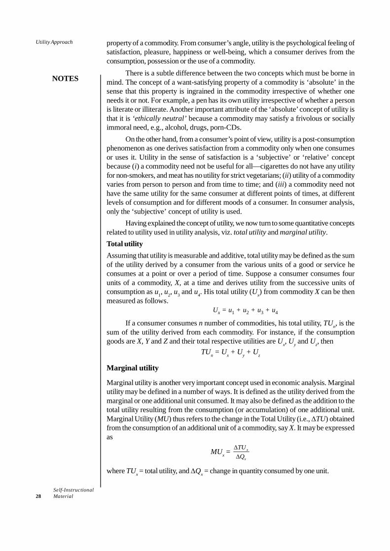
Self-Instructional28 Material
Utility Approach
NOTES
property of a commodity. From consumer’s angle, utility is the psychological feeling ofsatisfaction, pleasure, happiness or well-being, which a consumer derives from theconsumption, possession or the use of a commodity.
There is a subtle difference between the two concepts which must be borne inmind. The concept of a want-satisfying property of a commodity is ‘absolute’ in thesense that this property is ingrained in the commodity irrespective of whether oneneeds it or not. For example, a pen has its own utility irrespective of whether a personis literate or illiterate. Another important attribute of the ‘absolute’ concept of utility isthat it is ‘ethically neutral’ because a commodity may satisfy a frivolous or sociallyimmoral need, e.g., alcohol, drugs, porn-CDs.
On the other hand, from a consumer’s point of view, utility is a post-consumptionphenomenon as one derives satisfaction from a commodity only when one consumesor uses it. Utility in the sense of satisfaction is a ‘subjective’ or ‘relative’ conceptbecause (i) a commodity need not be useful for all—cigarettes do not have any utilityfor non-smokers, and meat has no utility for strict vegetarians; (ii) utility of a commodityvaries from person to person and from time to time; and (iii) a commodity need nothave the same utility for the same consumer at different points of times, at differentlevels of consumption and for different moods of a consumer. In consumer analysis,only the ‘subjective’ concept of utility is used.
Having explained the concept of utility, we now turn to some quantitative conceptsrelated to utility used in utility analysis, viz. total utility and marginal utility.Total utilityAssuming that utility is measurable and additive, total utility may be defined as the sumof the utility derived by a consumer from the various units of a good or service heconsumes at a point or over a period of time. Suppose a consumer consumes fourunits of a commodity, X, at a time and derives utility from the successive units ofconsumption as u1, u2, u3 and u4. His total utility (Ux) from commodity X can be thenmeasured as follows.
Ux = u1 + u2 + u3 + u4
If a consumer consumes n number of commodities, his total utility, TUn, is thesum of the utility derived from each commodity. For instance, if the consumptiongoods are X, Y and Z and their total respective utilities are Ux, Uy and Uz, then
TUn = Ux + Uy + Uz
Marginal utility
Marginal utility is another very important concept used in economic analysis. Marginalutility may be defined in a number of ways. It is defined as the utility derived from themarginal or one additional unit consumed. It may also be defined as the addition to thetotal utility resulting from the consumption (or accumulation) of one additional unit.Marginal Utility (MU) thus refers to the change in the Total Utility (i.e., ΔTU) obtainedfrom the consumption of an additional unit of a commodity, say X. It may be expressedas
MUx = x
x
TUQ
ΔΔ
where TUx = total utility, and ΔQx = change in quantity consumed by one unit.

Self-InstructionalMaterial 29
Utility Approach
NOTES
Another way of expressing marginal utility (MU), when the number of unitsconsumed is n, can be as follows.
MU of nth unit = TUn – TUn–1
2.3 LAW OF DIMINISHING MARGINAL UTILITY
The law of diminishing marginal utility is one of the fundamental laws of economics.This law states that as the quantity consumed of a commodity goes on increasing, theutility derived from each successive unit goes on diminishing, consumption of all othercommodities remaining the same. In simple words, when a person consumes more andmore units of a commodity per unit of time, e.g., ice cream, keeping the consumption ofall other commodities constant, the utility which he derives from each successive cup ofice cream goes on diminishing. This law applies to all kinds of consumer goods—durableand non-durable, sooner or later.
To illustrate the law of diminishing marginal utility, let us assume that a consumerconsumes only one commodity X, and that utility is measurable in quantitative terms.Let us also suppose that total and marginal utility schedules of commondity X aregiven as in Table 2.1. The law of diminishing marginal utility is illustrated numerically inTable 2.1 and graphically in Figure 2.1.
Table 2.1 Total and Marginal Utility Schedules for Commodity X
Units of commodity Total utility Marginal utilityX (TUx) (MUx)
1 30 30
2 50 20
3 60 10
4 65 5
5 60 – 5
6 45 – 15
As shown in Table 2.1, with the increase in the number of units of commodity Xconsumed per unit of time, TUx, increases but at a diminishing rate. The diminishingMUx is shown in the last column of Table 2.1. Figure 2.1 illustrates graphically the lawof diminishing MUx. The rate of increase in TUx as a result of increase in the number ofunits consumed is shown by the MUx curve in Figure 2.1. The downward slopingMUx curve shows that marginal utility goes on decreasing as consumption increases.At 4 units consumed, the TUx reaches its maximum level, the point of saturationmarked by point M. Beyond this point, MUx becomes negative and TUx begins todecline. The downward sloping MUx curve illustrates the law of diminishing marginalutility.
Check Your Progress
1. Define total utility.2. Define marginal
utility.
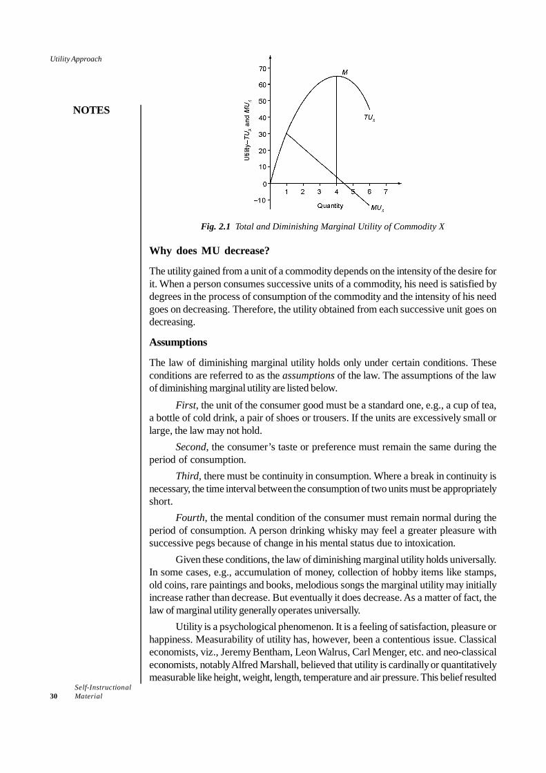
Self-Instructional30 Material
Utility Approach
NOTES
Fig. 2.1 Total and Diminishing Marginal Utility of Commodity X
Why does MU decrease?
The utility gained from a unit of a commodity depends on the intensity of the desire forit. When a person consumes successive units of a commodity, his need is satisfied bydegrees in the process of consumption of the commodity and the intensity of his needgoes on decreasing. Therefore, the utility obtained from each successive unit goes ondecreasing.
Assumptions
The law of diminishing marginal utility holds only under certain conditions. Theseconditions are referred to as the assumptions of the law. The assumptions of the lawof diminishing marginal utility are listed below.
First, the unit of the consumer good must be a standard one, e.g., a cup of tea,a bottle of cold drink, a pair of shoes or trousers. If the units are excessively small orlarge, the law may not hold.
Second, the consumer’s taste or preference must remain the same during theperiod of consumption.
Third, there must be continuity in consumption. Where a break in continuity isnecessary, the time interval between the consumption of two units must be appropriatelyshort.
Fourth, the mental condition of the consumer must remain normal during theperiod of consumption. A person drinking whisky may feel a greater pleasure withsuccessive pegs because of change in his mental status due to intoxication.
Given these conditions, the law of diminishing marginal utility holds universally.In some cases, e.g., accumulation of money, collection of hobby items like stamps,old coins, rare paintings and books, melodious songs the marginal utility may initiallyincrease rather than decrease. But eventually it does decrease. As a matter of fact, thelaw of marginal utility generally operates universally.
Utility is a psychological phenomenon. It is a feeling of satisfaction, pleasure orhappiness. Measurability of utility has, however, been a contentious issue. Classicaleconomists, viz., Jeremy Bentham, Leon Walrus, Carl Menger, etc. and neo-classicaleconomists, notably Alfred Marshall, believed that utility is cardinally or quantitativelymeasurable like height, weight, length, temperature and air pressure. This belief resulted

Self-InstructionalMaterial 31
Utility Approach
NOTES
in the cardinal utility concept. However, modern economists, most notably J.R. Hicksand R.G.D. Allen, hold the view that utility is not quantitatively measurable—it is notmeasurable in absolute terms. Utility can be expressed only ordinally or in terms of ‘lessthan’ or ‘more than’. It is, therefore, possible to list the goods and services in order oftheir preferability or desirability. For example, suppose a person prefers chocolate to icecream and ice cream to cold drink. He or she can express his/her preference as chocolate> ice cream > cold drink. But he cannot express his preference in quantitative terms.This is known as the ordinal concept of utility. Let us now look into the origin of the twoconcepts of utility and their use in the analysis of demand.
Cardinal utility
Some early psychological experiments on an individual’s responses to various stimuli ledneo-classical economists to believe that utility is measurable and cardinally quantifiable.This belief gave rise to the concept of cardinal utility. It implies that utility can be assigneda cardinal number like 1, 2, 3, etc. Neo-classical economists built up the theory ofconsumption on the assumption that utility is cardinally measurable. They coined andused a term ‘util’ meaning ‘units of utility’. In their measure of utility, they assumed (i)that one ‘util’ equals one unit of money, and (ii) that utility of money remains constant.
It has, however, been realized over time that absolute or cardinal measurementof utility is not possible. Difficulties in measuring utility have proved to beinsurmountable. Neither economists nor scientists have succeeded in devising a techniqueor an instrument for measuring the feeling of satisfaction, i.e., utility. Nor could anappropriate measure of unit be devised. Numerous factors affect the state of consumer’smood, which are impossible to determine and quantify. Utility is, therefore, notmeasurable in cardinal terms. Yet cardinal utility concept continues to remain anessential starting point in the analysis of consumer behaviour.
Ordinal utility
The modern economists have discarded the concept of cardinal utility and have insteademployed the concept of ordinal utility for analyzing consumer behaviour. The conceptof ordinal utility is based on the fact that it may not be possible for consumers toexpress the utility of a commodity in absolute or quantitative terms, but it is alwayspossible for a consumer to tell introspectively whether a commodity is more or less orequally useful when compared to another. For example, a consumer may not be able tosay that ice cream gives 5 utils and chocolate gives 10 utils. But he or she can alwaysspecify whether chocolate gives more or less utility than ice cream. This assumptionforms the basis of the ordinal theory of consumer behaviour.
While neo-classical economists maintained that cardinal measurement of utility ispractically possible and is meaningful in consumer analysis, modern economists maintainthat utility being a psychological phenomenon is inherently immeasurable, theoretically,conceptually as well as quantitatively. They also maintain that the concept of ordinalutility is a feasible concept and it meets the conceptual requirement of analyzing consumerbehaviour in the absence of any cardinal measures of utility.
Two Approaches to the Consumer Demand Analysis
Based on cardinal and ordinal concepts of utility, there are two approaches to the analysisof consumer behaviour.
Self-Instructional32 Material
Utility Approach
NOTES
• Cardinal utility approach, attributed to Alfred Marshall and his followers, isalso called the Neo-classical Approach.
• Ordinal utility approach, pioneered by J.R. Hicks, a Nobel laureate, and R.G.D.Allen, is also called the indifference curve analysis.
The two approaches are not in conflict with one another. In fact, they represent twolevels of sophistication in the analysis of consumer behaviour. Both the approachesare important for assessing and analyzing consumer demand for a commodity—be itfor thoretical purpose or for business decision-making, depending on the level ofsophistication required.
It is important to note in this regard that in spite of tremendous developments inconsumption theory based on ordinal utility, the classical demand theory based oncardinal utility has retained its appeal and applicability to the analysis of consumerbehaviour. Besides, the study of classical demand theory serves as a foundation forunderstanding the advanced theories of consumer behaviour. The study of classicaltheory of demand is of particular importance and contributes a great deal in managerialdecisions.
2.3.1 Analysis of Consumer Behaviour: Cardinal Utility Approach
The central theme of the consumption theory – be it based on ordinal utility or cardinalutility approach – is the utility maximizing behaviour of the consumer. The fundamentalpostulate of the consumption theory is that all the consumers—individuals andhouseholds—aim at utility maximization and all their decisions and actions asconsumers are directed towards utility maximization. The specific questions that theconsumption theory seeks to answer are:
• How does a consumer decide the optimum quantity of a commodity that he orshe chooses to consume, i.e., how does a consumer attain his/her equilibrium inrespect to each commodity?
• How does he or she allocate his/her disposable income between variouscommodities of consumption so that his/her total utility is maximized?
The theory of consumer behaviour seeks to answer these questions on the basis of thepostulates that consumers seek to maximize their total utility or satisfaction.
Assumptions
The theory of consumer behaviour based on the cardinal utility approach seeks toanswer the above questions on the basis of the following assumptions.
(i) Rationality: It is assumed that the consumer is a rational being in the sense thathe or she satisfies his/her wants in the order of their preference. That is, he orshe buys that commodity first which yields the highest utility and the last whichgives the least utility.
(ii) Limited money income: The consumer has a limited money income to spendon the goods and services he or she chooses to consume. Limitedness ofincome, along with utility maximization objective makes the choice betweengoods inevitable.
(iii) Maximization of satisfaction: Every rational consumer intends to maximizehis/her satisfaction from his/her given money income.
(iv) Utility is cardinally measurable: The cardinalists have assumed that utility iscardinally measurable and that utility of one unit of a commodity equals the

Self-InstructionalMaterial 33
Utility Approach
NOTES
units of money which a consumer is prepared to pay for it and that 1 util = 1 unitof money.
(v) Diminishing marginal utility: Following the law of diminishing marginal utility,it is assumed that the utility gained from the successive units of a commodityconsumed decreases as a person consumes them. This is an axiom of thetheory of consumer behaviour.
(vi) Constant marginal utility of money: The cardinal utility approach assumesthat marginal utility of money remains constant whatever the level of a consumer’sincome. This assumption is necessary to keep the scale of measuring rod ofutility fixed. It is important to recall in this regard that cardinalists used ‘money’as a measure of utility.
(vii) Utility is additive: Cardinalists assumed not only that utility is cardinallymeasurable but also that utility derived from various goods and servicesconsumed by a consumer can be added together to obtain the total utility.Suppose a consumer consumes X1, X2, X3,...Xn units of a commodity X andthat she/he derives U1, U2, U3 ... Un utils respectively, from the various units ofcommodity X consumed. Given the assumption, the total utility that the consumerderives form n units of commodity X can be expressed as
Un = U1(X1) + U2(X2) + U3(X3) + ... + Un(Xn)
Consumer’s equilibrium: Cardinal utility approach
Conceptually, a consumer reaches his equilibrium position when he has maximized thelevel of his satisfaction, given his resources and other conditions. Technically, a utility-maximizing consumer reaches his equilibrium position when allocation of his expenditureis such that the last penny spent on each commodity yields the same utility. In order toexplain how a consumer reaches his equilibrium, we begin with the simplest case of aconsumer consuming only one commodity. The analysis will then be extended toexplain equilibrium of a consumer consuming several goods.
(i) Consumer’s equilibrium: One-commodity model: Suppose that a consumerwith a given money income consumes only one commodity, X. Since both hismoney income and commodity X have utility for him, he can either spend hismoney income on commodity X or retain it in the form of asset. If the marginalutility of commodity X, (MUx) is greater than marginal utility of money (MUm)1,a utility-maximizing consumer will exchange his money income for thecommodity. By assumption, MUx is subject to diminishing returns (assumptionv), whereas marginal utility of money (MUm) remains constant (assumption vi).Therefore, the consumer will spend his money income on commodity X solong as MUx > Px(MUm), Px being the price of commodity X and MUm = 1(constant). The utility-maximizing consumer reaches his equilibrium, i.e., thelevel of maximum satisfaction, where
MUx = Px (MUm)
Alternatively, the consumer reaches equilibrium where
( )x
x m
MUP MU
= 1
Consumer’s equilibrium in a single commodity model is graphically illustratedin Figure 2.2. The horizontal line marked Px (MUm) shows the constant utility ofmoney weighted by the price of commodity X (i.e., Px) and MUx curve represents
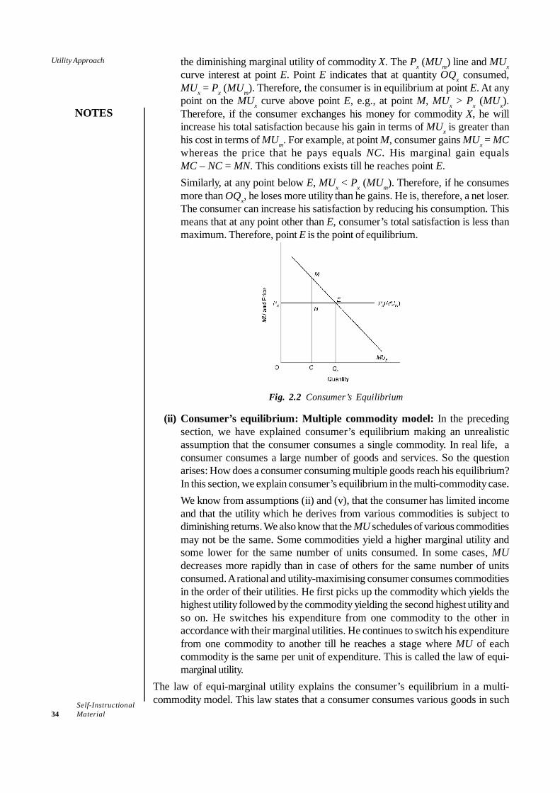
Self-Instructional34 Material
Utility Approach
NOTES
the diminishing marginal utility of commodity X. The Px (MUm) line and MUxcurve interest at point E. Point E indicates that at quantity OQx consumed,MUx = Px (MUm). Therefore, the consumer is in equilibrium at point E. At anypoint on the MUx curve above point E, e.g., at point M, MUx > Px (MUx).Therefore, if the consumer exchanges his money for commodity X, he willincrease his total satisfaction because his gain in terms of MUx is greater thanhis cost in terms of MUm. For example, at point M, consumer gains MUx = MCwhereas the price that he pays equals NC. His marginal gain equalsMC – NC = MN. This conditions exists till he reaches point E.Similarly, at any point below E, MUx < Px (MUm). Therefore, if he consumesmore than OQx, he loses more utility than he gains. He is, therefore, a net loser.The consumer can increase his satisfaction by reducing his consumption. Thismeans that at any point other than E, consumer’s total satisfaction is less thanmaximum. Therefore, point E is the point of equilibrium.
Fig. 2.2 Consumer’s Equilibrium
(ii) Consumer’s equilibrium: Multiple commodity model: In the precedingsection, we have explained consumer’s equilibrium making an unrealisticassumption that the consumer consumes a single commodity. In real life, aconsumer consumes a large number of goods and services. So the questionarises: How does a consumer consuming multiple goods reach his equilibrium?In this section, we explain consumer’s equilibrium in the multi-commodity case.We know from assumptions (ii) and (v), that the consumer has limited incomeand that the utility which he derives from various commodities is subject todiminishing returns. We also know that the MU schedules of various commoditiesmay not be the same. Some commodities yield a higher marginal utility andsome lower for the same number of units consumed. In some cases, MUdecreases more rapidly than in case of others for the same number of unitsconsumed. A rational and utility-maximising consumer consumes commoditiesin the order of their utilities. He first picks up the commodity which yields thehighest utility followed by the commodity yielding the second highest utility andso on. He switches his expenditure from one commodity to the other inaccordance with their marginal utilities. He continues to switch his expenditurefrom one commodity to another till he reaches a stage where MU of eachcommodity is the same per unit of expenditure. This is called the law of equi-marginal utility.
The law of equi-marginal utility explains the consumer’s equilibrium in a multi-commodity model. This law states that a consumer consumes various goods in such

Self-InstructionalMaterial 35
Utility Approach
NOTES
quantities that the MU derived per unit of expenditure from each good is the same. Inother words, a rational consumer spends his income on various goods he consumes insuch a manner that each rupee spent on each good yields the same MU.
Let us now explain consumer’s equilibrium in a multi-commodity model. For thesake of simplicity, however, we consider only a two-commodity case. Suppose that aconsumer consumes only two commodities, X and Y, their prices being Px and Pyrespectively. Following the equilibrium rule of the single commodity case, the consumerwill spend his income on commodities X and Y in such proportions that
MUx = Px (MUm)and MUy = Py (MUm)
Given these conditions, the consumer’s equilibrium can be expressed as
( )x
x m
MUP MU
= 1 = ( )
y
y m
MUP MU
...(2.1)
Since, according to assumption (vi), MU of each unit of money (or each rupee) is constantat 1, Eq. (2.1) can be rewritten as
x
x
MUP
= y
y
MUP
...(2.2)
or x
y
MUMU = x
y
PP ...(2.3)
Equation (2.2) leads to the conclusion that the consumer reaches his equilibrium whenthe marginal utility derived from each rupee spent on the two commodities X and Y isthe same. Eq. (2.3) reveals that a consumer is in equilibrium when MU ratio of any twogoods equals their price ratio.
The two-commodity case can be used to generalize the rule for consumer’sequilibrium for a consumer consuming a large number of goods and services with agiven income and at different prices. Supposing, a consumer consumes A to Z goodsand services, his equilibrium condition may be expressed as
mZ
Z
B
B
A
A MUPMU
PMU
PMU
==== ...(2.4)
Equation (2.4) gives the Law of Equi-marginal Utility.It is important to note that, in order to achieve his equilibrium, what a utility
maximizing consumer intends to equalize is not the marginal utility of each commodityhe consumes, but the marginal utility per unit of his money expenditure on variousgoods and services.
In preceding sections, we have explained the utility maximizing behaviour of theconsumer and the concept of and conditions for consumer’s equilibrium. Analysis ofconsumer’s equilibrium provides a convenient basis for the derivation of the individualdemand curve for a commodity. Marshall was the first economist to explicitly derive thedemand curve from the consumer’s utility function.2 As shown above, a consumerconsuming only one commodity, say X, is in equilibrium where MUx = Px (MUm). Usingthis equilibrium condition, consumer’s equilibrium has been illustrated in Figure 2.2. Thesame logic can be used to derive consumer’s demand curve for commodity X.
The derivation of individual demand for the commodity X is illustrated in Figure2.3 (a) and (b). Suppose that the consumer is in equilibrium at point E1. It means that
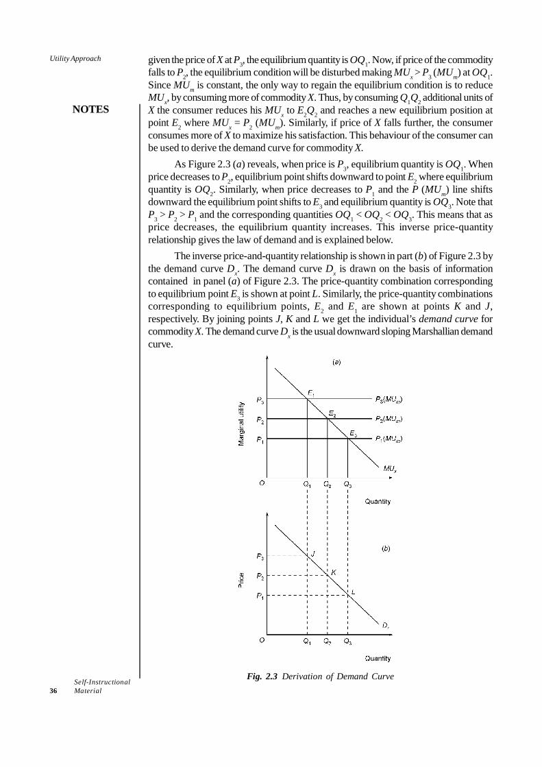
Self-Instructional36 Material
Utility Approach
NOTES
given the price of X at P3, the equilibrium quantity is OQ1. Now, if price of the commodityfalls to P2, the equilibrium condition will be disturbed making MUx > P3 (MUm) at OQ1.Since MUm is constant, the only way to regain the equilibrium condition is to reduceMUx, by consuming more of commodity X. Thus, by consuming Q1Q2 additional units ofX the consumer reduces his MUx to E2Q2 and reaches a new equilibrium position atpoint E2 where MUx = P2 (MUm). Similarly, if price of X falls further, the consumerconsumes more of X to maximize his satisfaction. This behaviour of the consumer canbe used to derive the demand curve for commodity X.
As Figure 2.3 (a) reveals, when price is P3, equilibrium quantity is OQ1. Whenprice decreases to P2, equilibrium point shifts downward to point E2 where equilibriumquantity is OQ2. Similarly, when price decreases to P1 and the P (MUm) line shiftsdownward the equilibrium point shifts to E3 and equilibrium quantity is OQ3. Note thatP3 > P2 > P1 and the corresponding quantities OQ1 < OQ2 < OQ3. This means that asprice decreases, the equilibrium quantity increases. This inverse price-quantityrelationship gives the law of demand and is explained below.
The inverse price-and-quantity relationship is shown in part (b) of Figure 2.3 bythe demand curve Dx. The demand curve Dx is drawn on the basis of informationcontained in panel (a) of Figure 2.3. The price-quantity combination correspondingto equilibrium point E3 is shown at point L. Similarly, the price-quantity combinationscorresponding to equilibrium points, E2 and E1 are shown at points K and J,respectively. By joining points J, K and L we get the individual’s demand curve forcommodity X. The demand curve Dx is the usual downward sloping Marshallian demandcurve.
Fig. 2.3 Derivation of Demand Curve

Self-InstructionalMaterial 37
Utility Approach
NOTES
Demand under Variable MUm: We have explained above the consumer’s equilibriumand derived his demand curve under the assumption that MUm remains constant. Thisanalysis holds even if MUm is assumed to be variable. This can be explained as follows.
Suppose MUm is variable—it decreases with increase in stock of money and viceversa. Under this condition, if price of a commodity falls and the consumer buys only asmany units as he did before the fall in price, he saves some money on this commodity. Asa result his stock of money increases and his MUm decreases, whereas MUx remainsunchanged because his stock of commodity remains unchanged. As a result, his MUxexceeds his MUm. When a consumer exchanges money for commodity, his stock ofmoney decreases and stock of commodity increases. As a result, MUm increases andMUx decreases. The consumer, therefore, exchanges money for commodity until MUx= MUm. Consequently, demand for a commodity increases when its price falls.
2.3.2 Analysis of Consumer Behaviour: Ordinal Utility Approach
Unlike Marshall, the modern economists, Hicks in particular, have used the ordinal utilityconcept to analyze consumer’s behaviour. This is called ‘ordinal utility approach’. Hickshas used a different tool of analysis called ‘indifference curve’ to analyze consumerbehaviour. In this section, we will first explain the ‘indifference curve’ and then explainconsumer’s behaviour through the indifference curve technique. Let us first look at theassumptions of the ordinal utility approach.
Assumptions of Ordinal Utility Theory
1. Rationality: The consumer is assumed to be a rational being. Rationality meansthat a consumer aims at maximizing his total satisfaction given his income andprices of the goods and services that he consumes and his decisions areconsistent with this objective.
2. Ordinal utility: Indifference curve analysis assumes that utility is only ordinallyexpressible. That is, the consumer is only able to express the order of hispreference for different baskets of goods.
3. Transitivity and consistency of choice: Consumer’s choices are assumed tobe transitive. Transitivity of choice means that if a consumer prefers A to B andB to C, he must prefer A to C. Or, if he treats A = B and B = C, he must treatA = C. Consistency of choice means that if he prefers A to B in one period, hedoes not prefer B to A in another period or even treat them as equal.
4. Nonsatiety: It is also assumed that the consumer is never over-supplied withgoods in question. That is, he has not reached the point of saturation in case ofany commodity. Therefore, a consumer always prefers a larger quantity of allthe goods.
5. Diminishing marginal rate of substitution: The marginal rate of substitutionis the rate at which a consumer is willing to substitute one commodity (X) foranother (Y) so that his total satisfaction remains the same. The marginal rate ofsubstitution is given as ΔY/ΔX. The ordinal utility approach assumes thatΔY/ΔX goes on decreasing when a consumer continues to substitute X for Y.(We will discuss marginal rate of substitution in detail in the subsequent section).
2.3.3 Meaning and Nature of Indifference Curve
An indifference curve may be defined as the locus of points each representing adifferent combination of two substitute goods, which yield the same utility or level of
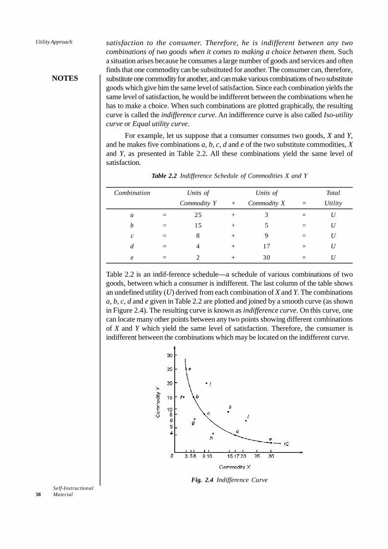
Self-Instructional38 Material
Utility Approach
NOTES
satisfaction to the consumer. Therefore, he is indifferent between any twocombinations of two goods when it comes to making a choice between them. Sucha situation arises because he consumes a large number of goods and services and oftenfinds that one commodity can be substituted for another. The consumer can, therefore,substitute one commodity for another, and can make various combinations of two substitutegoods which give him the same level of satisfaction. Since each combination yields thesame level of satisfaction, he would be indifferent between the combinations when hehas to make a choice. When such combinations are plotted graphically, the resultingcurve is called the indifference curve. An indifference curve is also called Iso-utilitycurve or Equal utility curve.
For example, let us suppose that a consumer consumes two goods, X and Y,and he makes five combinations a, b, c, d and e of the two substitute commodities, Xand Y, as presented in Table 2.2. All these combinations yield the same level ofsatisfaction.
Table 2.2 Indifference Schedule of Commodities X and Y
Combination Units of Units of TotalCommodity Y + Commodity X = Utility
a = 25 + 3 = Ub = 15 + 5 = Uc = 8 + 9 = Ud = 4 + 17 = U
e = 2 + 30 = U
Table 2.2 is an indif-ference schedule—a schedule of various combinations of twogoods, between which a consumer is indifferent. The last column of the table showsan undefined utility (U) derived from each combination of X and Y. The combinationsa, b, c, d and e given in Table 2.2 are plotted and joined by a smooth curve (as shownin Figure 2.4). The resulting curve is known as indifference curve. On this curve, onecan locate many other points between any two points showing different combinationsof X and Y which yield the same level of satisfaction. Therefore, the consumer isindifferent between the combinations which may be located on the indifferent curve.
Fig. 2.4 Indifference Curve
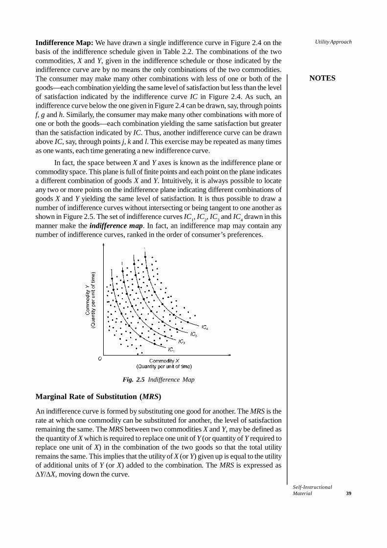
Self-InstructionalMaterial 39
Utility Approach
NOTES
Indifference Map: We have drawn a single indifference curve in Figure 2.4 on thebasis of the indifference schedule given in Table 2.2. The combinations of the twocommodities, X and Y, given in the indifference schedule or those indicated by theindifference curve are by no means the only combinations of the two commodities.The consumer may make many other combinations with less of one or both of thegoods—each combination yielding the same level of satisfaction but less than the levelof satisfaction indicated by the indifference curve IC in Figure 2.4. As such, anindifference curve below the one given in Figure 2.4 can be drawn, say, through pointsf, g and h. Similarly, the consumer may make many other combinations with more ofone or both the goods—each combination yielding the same satisfaction but greaterthan the satisfaction indicated by IC. Thus, another indifference curve can be drawnabove IC, say, through points j, k and l. This exercise may be repeated as many timesas one wants, each time generating a new indifference curve.
In fact, the space between X and Y axes is known as the indifference plane orcommodity space. This plane is full of finite points and each point on the plane indicatesa different combination of goods X and Y. Intuitively, it is always possible to locateany two or more points on the indifference plane indicating different combinations ofgoods X and Y yielding the same level of satisfaction. It is thus possible to draw anumber of indifference curves without intersecting or being tangent to one another asshown in Figure 2.5. The set of indifference curves IC1, IC2, IC3 and IC4 drawn in thismanner make the indifference map. In fact, an indifference map may contain anynumber of indifference curves, ranked in the order of consumer’s preferences.
Fig. 2.5 Indifference Map
Marginal Rate of Substitution (MRS)
An indifference curve is formed by substituting one good for another. The MRS is therate at which one commodity can be substituted for another, the level of satisfactionremaining the same. The MRS between two commodities X and Y, may be defined asthe quantity of X which is required to replace one unit of Y (or quantity of Y required toreplace one unit of X) in the combination of the two goods so that the total utilityremains the same. This implies that the utility of X (or Y) given up is equal to the utilityof additional units of Y (or X) added to the combination. The MRS is expressed asΔY/ΔX, moving down the curve.

Self-Instructional40 Material
Utility Approach
NOTES
MRS goes on diminishing: The basic postulate of ordinal utility theory is thatMRSy, x (or MRSx, y) decreases. It means that the quantity of a commodity that aconsumer is willing to sacrifice for an additional unit of another goes on decreasingwhen he goes on substituting one commodity for another. The diminishing MRSx, yobtained from combinations of X and Y given in Table 2.2 is presented in Table 2.3.
Table 2.3 The Diminishing MRS between Commodities X and Y
Indifference Points Combinations Change in Y Change in X MRSy, x
Y + X (– ΔY) (ΔX) (ΔY/ΔX)
a 25 + 3 – – –b 15 + 5 – 10 2 – 5.00c 8 + 9 – 7 4 – 1.75d 4 + 17 – 4 8 – 0.50
e 2 + 30 – 2 13 – 0.15
As Table 2.3 shows, when the consumer moves from point a to b on his indifferencecurve (Figure 2.4) he gives up 10 units of commodity Y and gets only 3 units ofcommodity X, so that
,10 5.002y x
YMRSX
−Δ −= = = −
Δ
As he moves down from point b to c, he loses 7 units of Y and gains 4 units of X,giving
,7 1.75
4y xYMRS
X−Δ −
= = = −Δ
Note that as the consumer moves from point a to b and from point b to c, the MRSdecreases from –5.00 to –1.75. The MRSy, x goes on decreasing as the consumermoves further down along the indifference curve, from point c through d and e. Thediminishing marginal rate of substitution causes the indifference curves to be convexto the origin.
Why Does MRS Diminish?
The MRS diminishes along the IC curve because, in most cases, no two goods areperfect substitutes for one another. In case any two goods are perfect substitutes, theindifference curve will be a straight line having a negative slope showing constantMRS. Since goods are not perfect substitutes, the subjective value attached to theadditional quantity (i.e., subjective MU) of a commodity decreases fast in relation tothe other commodity whose total quantity is decreasing. Therefore, when the quantityof one commodity (X) increases and that of the other (Y) decreases, the subjectiveMU of Y increases and that of X decreases. Therefore, the consumer becomesincreasingly unwilling to sacrifice more units of Y for one unit of X. But, if he isrequired to sacrifice additional units of Y, he will demand increasing units of X tomaintain the level of his satisfaction. As a result, the MRS decreases.
Furthermore, when combination of two goods at a point on the indifferencecurve is such that it includes a large quantity of one commodity (Y) and a smallquantity of the other commodity (X), then consumer’s capacity to sacrifice Y is greaterthan to sacrifice X. Therefore, he can sacrifice a larger quantity of Y in favour of a
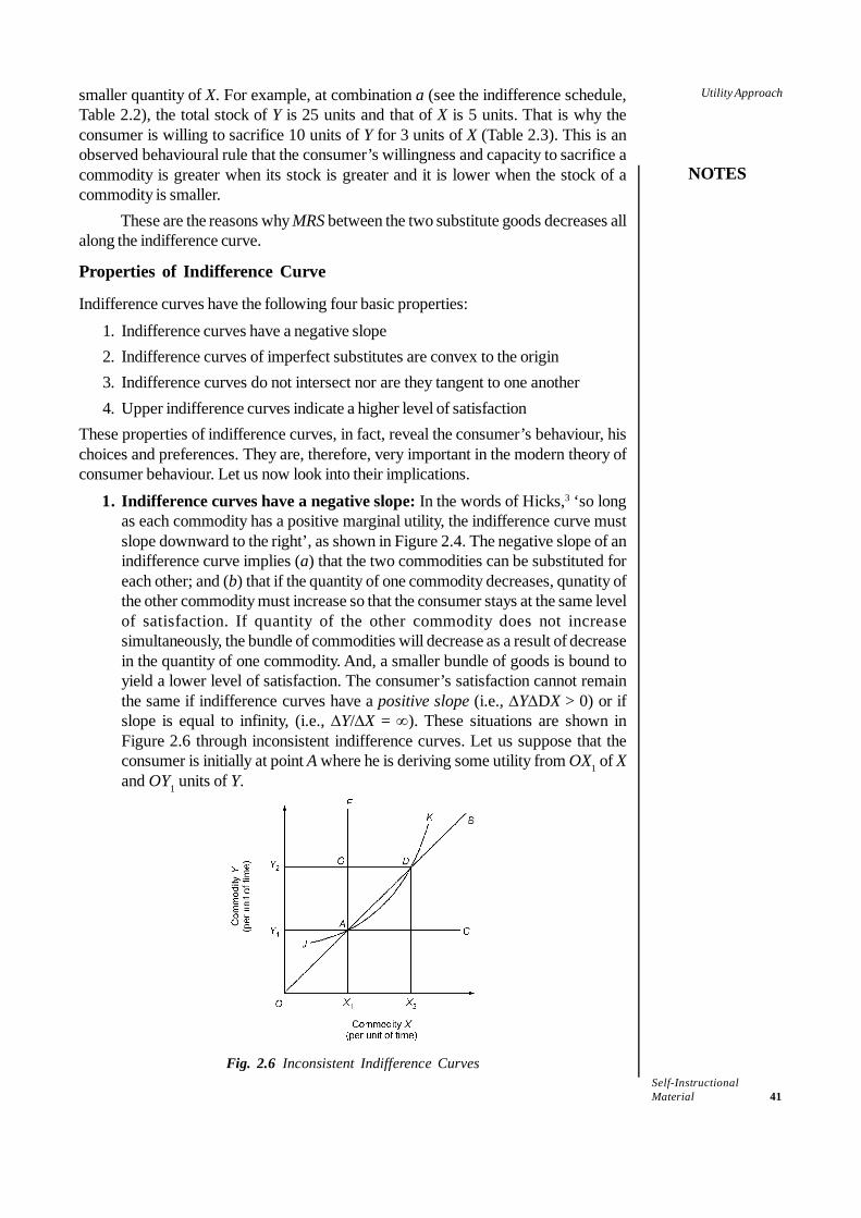
Self-InstructionalMaterial 41
Utility Approach
NOTES
smaller quantity of X. For example, at combination a (see the indifference schedule,Table 2.2), the total stock of Y is 25 units and that of X is 5 units. That is why theconsumer is willing to sacrifice 10 units of Y for 3 units of X (Table 2.3). This is anobserved behavioural rule that the consumer’s willingness and capacity to sacrifice acommodity is greater when its stock is greater and it is lower when the stock of acommodity is smaller.
These are the reasons why MRS between the two substitute goods decreases allalong the indifference curve.
Properties of Indifference Curve
Indifference curves have the following four basic properties:1. Indifference curves have a negative slope2. Indifference curves of imperfect substitutes are convex to the origin3. Indifference curves do not intersect nor are they tangent to one another4. Upper indifference curves indicate a higher level of satisfaction
These properties of indifference curves, in fact, reveal the consumer’s behaviour, hischoices and preferences. They are, therefore, very important in the modern theory ofconsumer behaviour. Let us now look into their implications.
1. Indifference curves have a negative slope: In the words of Hicks,3 ‘so longas each commodity has a positive marginal utility, the indifference curve mustslope downward to the right’, as shown in Figure 2.4. The negative slope of anindifference curve implies (a) that the two commodities can be substituted foreach other; and (b) that if the quantity of one commodity decreases, qunatity ofthe other commodity must increase so that the consumer stays at the same levelof satisfaction. If quantity of the other commodity does not increasesimultaneously, the bundle of commodities will decrease as a result of decreasein the quantity of one commodity. And, a smaller bundle of goods is bound toyield a lower level of satisfaction. The consumer’s satisfaction cannot remainthe same if indifference curves have a positive slope (i.e., ΔYΔDX > 0) or ifslope is equal to infinity, (i.e., ΔY/ΔX = ∞). These situations are shown inFigure 2.6 through inconsistent indifference curves. Let us suppose that theconsumer is initially at point A where he is deriving some utility from OX1 of Xand OY1 units of Y.
Fig. 2.6 Inconsistent Indifference Curves

Self-Instructional42 Material
Utility Approach
NOTES
If an indifference curve has a positive slope (i.e., ΔY/ΔX > 0), as shown by theline OB and curve JK, it implies that upward movement along the line or thecurve increases the combination of the two goods but the consumer is equallysatisfied with larger and smaller baskets of X and Y. This means an irrationalbehaviour of the consumer. For example, if the consumer moves from point Ato D, the combination of the two goods increases by Y1Y2 of Y and X1X2 of X.Unless MU of Y1Y2 and X1X2 are equal to zero, the level of satisfaction is boundto increase whereas on an indifference curve, the total utility is supposed toremain the same. Therefore, line OB and curve JK cannot be indifference curves.Similarly, in the case of a vertical indifference line, FX1, the movement frompoint A to G means an increase in the quantity of Y by Y1Y2, while quantity of Xremains the same, OX1. If MU of Y1Y2 > 0, the total utility will increase. So is thecase if an indifference curve takes the shape of a horizontal line, like Y1C.
2. Indifference curves are convex to origin: Indifference curves are not onlynegatively sloped, but are also convex to the origin as shown in Figure 2.4. Theconvexity of the indifference curves implies two properties:• the two commodities are imperfect substitutes for one another, and• the marginal rate of substitution (MRS) between the two goods decreases as
a consumer moves along an indifference curve. This characteristic ofindifference curve is based on the postulate of diminishing marginal rate ofsubstitution.The postulate of diminishing MRS, as mentioned above, states an observedfact that if a consumer substitutes one commodity (X) for another (Y), hiswillingness to sacrifice more units of Y for one additional unit of X decreases,as quantity of Y decreases. There are two reasons for this: (i) no twocommodities are perfect substitutes for one another, and (ii) MU of acommodity increases as its quantity decreases and vice versa, and, therefore,more and more units of the other commodity are needed to keep the totalutility constant.
3. Indifference curves can neither intersect nor be tangent with one another:If two indifference curves intersect or are tangent with one another, it will yieldtwo impossible conclusions: (i) that two equal combinations of two goodsyield two different levels of satisfaction, and (ii) that two different combinations—one being larger than the other–yield the same level of satisfaction. Suchconditions are impossible if the consumer’s subjective valuation of a commodityis greater than zero. Besides, if two indifference curves intersect, it would meannegation of consistency or transitivity assumption in consumer’s preferences.Let us now see what happens when two indifference curves, IC and IC′, intersecteach other at point A as shown in Figure 2.7. Point A falls on both the indifferencecurves, IC and IC′. It means that the same basket of goods (OM of X + AM ofY) yields different levels of utility below and above point A on the sameindifference curve. This implies inconsistency in consumer’s choice. Theinconsistency that two different baskets of X and Y yield the same level of utilitycan be proved as follows. Consider two other points—point B on indifferencecurve IC′ and point C on indifference curve IC both being on a vertical line.

Self-InstructionalMaterial 43
Utility Approach
NOTES
Fig. 2.7 Intersecting Indifference Curves
Points A, B and C represent three different combinations of commodities X and Y.Let us call these combinations as A, B and C, respectively. Note that combinationA is common to both the indifference curves. Therefore, the intersection of thetwo ICs implies that in terms of utility,
A = B (both combinations being on IC′)and A = C (both combinations being on IC)∴ B = C (both falling on different ICs)
But if B = C, it would mean that in terms of utility,ON of X + BN of Y = ON of X + CN of Y
But, note that ‘ON of X’ is common to both the sides. Therefore it means thatBN of Y = CN of Y. But as Figure 2.7 shows, BN > CN. Therefore, combinationsB and C cannot be equal in terms of satisfaction. The intersection, therefore,violates the transitivity rule which is a logical necessity in indifference curveanalysis. The same reasoning is applicable when two indifference curves aretangent with each other.
4. Upper indifference curves represent a higher level of satisfaction thanthe lower ones: An indifference curve placed above and to the right of anotherrepresents a higher level of satisfaction than the lower one. In Figure 2.8,indifference curve IC2 is placed above the curve IC1. Therefore, IC2 representsa higher level of satisfaction. The reason is that an upper indifference curvecontains all along its length a larger quantity of one or both the goods than thelower indifference curve. And a larger quantity of a commodity is supposed toyield a greater satisfaction than the smaller quantity of it, provided MU > 0.
Fig. 2.8 Comparison between Lower and Upper Indifference Curves
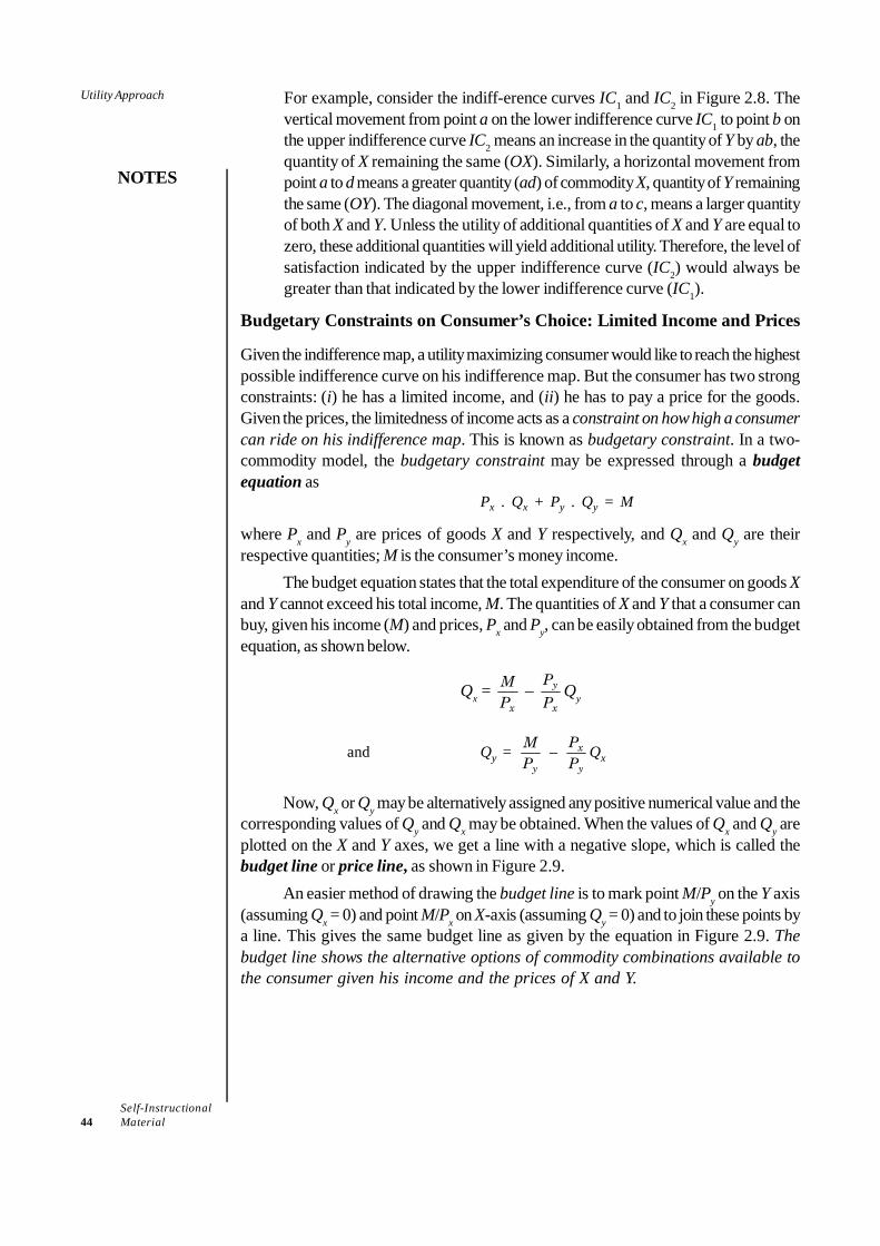
Self-Instructional44 Material
Utility Approach
NOTES
For example, consider the indiff-erence curves IC1 and IC2 in Figure 2.8. Thevertical movement from point a on the lower indifference curve IC1 to point b onthe upper indifference curve IC2 means an increase in the quantity of Y by ab, thequantity of X remaining the same (OX). Similarly, a horizontal movement frompoint a to d means a greater quantity (ad) of commodity X, quantity of Y remainingthe same (OY). The diagonal movement, i.e., from a to c, means a larger quantityof both X and Y. Unless the utility of additional quantities of X and Y are equal tozero, these additional quantities will yield additional utility. Therefore, the level ofsatisfaction indicated by the upper indifference curve (IC2) would always begreater than that indicated by the lower indifference curve (IC1).
Budgetary Constraints on Consumer’s Choice: Limited Income and Prices
Given the indifference map, a utility maximizing consumer would like to reach the highestpossible indifference curve on his indifference map. But the consumer has two strongconstraints: (i) he has a limited income, and (ii) he has to pay a price for the goods.Given the prices, the limitedness of income acts as a constraint on how high a consumercan ride on his indifference map. This is known as budgetary constraint. In a two-commodity model, the budgetary constraint may be expressed through a budgetequation as
Px . Qx + Py . Qy = M
where Px and Py are prices of goods X and Y respectively, and Qx and Qy are theirrespective quantities; M is the consumer’s money income.
The budget equation states that the total expenditure of the consumer on goods Xand Y cannot exceed his total income, M. The quantities of X and Y that a consumer canbuy, given his income (M) and prices, Px and Py, can be easily obtained from the budgetequation, as shown below.
Qx = MPx
– PP
y
xQy
and Qy = MPy
– PP
x
yQx
Now, Qx or Qy may be alternatively assigned any positive numerical value and thecorresponding values of Qy and Qx may be obtained. When the values of Qx and Qy areplotted on the X and Y axes, we get a line with a negative slope, which is called thebudget line or price line, as shown in Figure 2.9.
An easier method of drawing the budget line is to mark point M/Py on the Y axis(assuming Qx = 0) and point M/Px on X-axis (assuming Qy = 0) and to join these points bya line. This gives the same budget line as given by the equation in Figure 2.9. Thebudget line shows the alternative options of commodity combinations available tothe consumer given his income and the prices of X and Y.
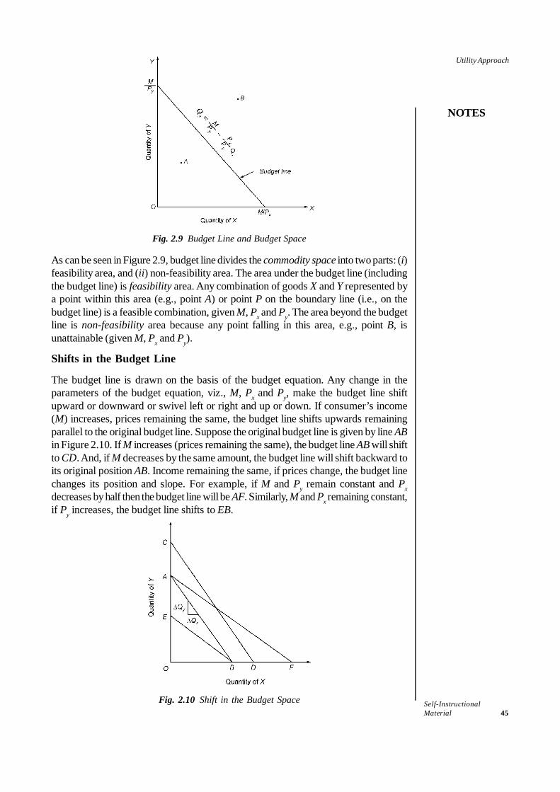
Self-InstructionalMaterial 45
Utility Approach
NOTES
Fig. 2.9 Budget Line and Budget Space
As can be seen in Figure 2.9, budget line divides the commodity space into two parts: (i)feasibility area, and (ii) non-feasibility area. The area under the budget line (includingthe budget line) is feasibility area. Any combination of goods X and Y represented bya point within this area (e.g., point A) or point P on the boundary line (i.e., on thebudget line) is a feasible combination, given M, Px and Py. The area beyond the budgetline is non-feasibility area because any point falling in this area, e.g., point B, isunattainable (given M, Px and Py).
Shifts in the Budget Line
The budget line is drawn on the basis of the budget equation. Any change in theparameters of the budget equation, viz., M, Px and Py, make the budget line shiftupward or downward or swivel left or right and up or down. If consumer’s income(M) increases, prices remaining the same, the budget line shifts upwards remainingparallel to the original budget line. Suppose the original budget line is given by line ABin Figure 2.10. If M increases (prices remaining the same), the budget line AB will shiftto CD. And, if M decreases by the same amount, the budget line will shift backward toits original position AB. Income remaining the same, if prices change, the budget linechanges its position and slope. For example, if M and Py remain constant and Pxdecreases by half then the budget line will be AF. Similarly, M and Px remaining constant,if Py increases, the budget line shifts to EB.
Fig. 2.10 Shift in the Budget Space

Self-Instructional46 Material
Utility Approach
NOTES
Slope of the Budget Line
Another important aspect of the budget line that matters in determining a consumer’sequilibrium is its slope. The slope of the budget line (AB) in Figure 2.10, is given as
y
x
Q OAQ OB
Δ=
Δ
Since OA = M/Py (when X = 0) and OB = M/Px (when Y = 0), the slope of the budgetline AB in Figure 2.10 may be rewritten as
OAOB
= y x
x y
M P PM P P
=
Thus, the slope of the budget line is the same as the price ratio of the two commodities.
2.3.4 Consumer’s Equilibrium: Ordinal Utility Approach
Now that we have discussed the indifference map and the budget line, we turn toanalyze consumer’s equilibrium. As noted earlier, a consumer attains his equilibriumwhen he maximizes his total utility, given his income and market prices of the goodsand services that he consumes. The ordinal utility approach specifies two conditionsfor the consumer’s equilibrium:
• Necessary or the first order condition, and• Supplementary or the second order condition.
In a two-commodity model, the necessary or the first order condition under ordinalutility approach is the same as equilibrium condition under cardinal utility approach. Itis given Eq. (2.2) as
MUMU
x
y =
PP
x
y
Since, by implication, MUx/MUy = MRSx, y, the necessary condition of equilibriumunder ordinal utility approach can be written as
MRSx, y = MUMU
x
y = P
Px
y
This is a necessary but not a sufficient condition of consumer’s equilibrium. Thesecond order or supplementary condition requires that the necessary condition befulfilled at the highest possible indifference curve.
Consumer’s equilibrium is illustrated in Figure 2.11. The indifference curvesIC1, IC2 and IC3 present a hypothetical indifference map of the consumer. The line ABis the hypothetical budget line. Both the budget line AB and the indifference curve IC2pass through point E. Therefore, the slopes of the indifference curve IC2 and thebudget line (AB) are equal. Thus, both the necessary and supplementary conditionsare fulfilled at point E. Therefore, consumer is in equilibrium at point E. This point canbe proved as follows.We know that between any two points on an indifferent curve,
ΔY × MUy = ΔX × MUx
and, therefore, the slope of an indifference curve is given byYX
ΔΔ
= x
y
MUMU = MRSy, x
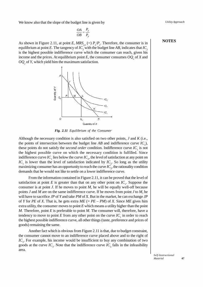
Self-InstructionalMaterial 47
Utility Approach
NOTES
We know also that the slope of the budget line is given by
y
y
POAOB P
=
As shown in Figure 2.11, at point E, MRSy,x (=) Px/Py. Therefore, the consumer is inequilibrium at point E. The tangency of IC2 with the budget line AB, indicates that IC2is the highest possible indifference curve which the consumer can reach, given hisincome and the prices. At equilibrium point E, the consumer consumes OQx of X andOQy of Y, which yield him the maximum satisfaction.
Fig. 2.11 Equilibrium of the Consumer
Although the necessary condition is also satisfied on two other points, J and K (i.e.,the points of intersection between the budget line AB and indifference curve IC1),these points do not satisfy the second order condition. Indifference curve IC1 is notthe highest possible curve on which the necessary condition is fulfilled. Sinceindifference curve IC1 lies below the curve IC2, the level of satisfaction at any point onIC1 is lower than the level of satisfaction indicated by IC2. So long as the utilitymaximizing consumer has an opportunity to reach the curve IC2, the rationality conditiondemands that he would not like to settle on a lower indifference curve.
From the information contained in Figure 2.11, it can be proved that the level ofsatisfaction at point E is greater than that on any other point on IC1. Suppose theconsumer is at point J. If he moves to point M, he will be equally well-off becausepoints J and M are on the same indifference curve. If he moves from point J to M, hewill have to sacrifice JP of Y and take PM of X. But in the market, he can exchange JPof Y for PE of X. That is, he gets extra ME (= PE – PM) of X. Since ME gives himextra utility, the consumer moves to point E which means a utility higher than the pointM. Therefore, point E is preferable to point M. The consumer will, therefore, have atendency to move to point E from any other point on the curve IC1 in order to reachthe highest possible indifference curve, all other things (taste, preference and prices ofgoods) remaining the same.
Another fact which is obvious from Figure 2.11 is that, due to budget constraint,the consumer cannot move to an indifference curve placed above and to the right ofIC2. For example, his income would be insufficient to buy any combination of twogoods at the curve IC3. Note that the indifference curve IC3 falls in the infeasibilityarea.
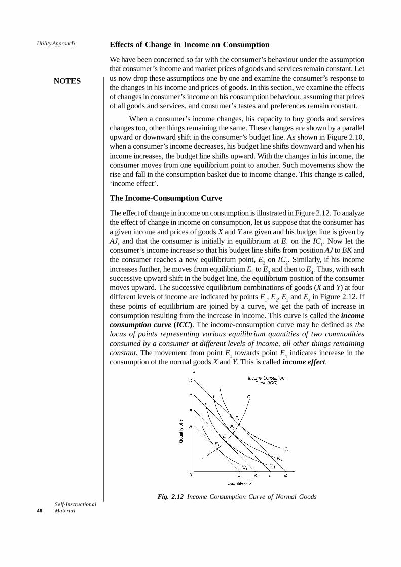
Self-Instructional48 Material
Utility Approach
NOTES
Effects of Change in Income on Consumption
We have been concerned so far with the consumer’s behaviour under the assumptionthat consumer’s income and market prices of goods and services remain constant. Letus now drop these assumptions one by one and examine the consumer’s response tothe changes in his income and prices of goods. In this section, we examine the effectsof changes in consumer’s income on his consumption behaviour, assuming that pricesof all goods and services, and consumer’s tastes and preferences remain constant.
When a consumer’s income changes, his capacity to buy goods and serviceschanges too, other things remaining the same. These changes are shown by a parallelupward or downward shift in the consumer’s budget line. As shown in Figure 2.10,when a consumer’s income decreases, his budget line shifts downward and when hisincome increases, the budget line shifts upward. With the changes in his income, theconsumer moves from one equilibrium point to another. Such movements show therise and fall in the consumption basket due to income change. This change is called,‘income effect’.
The Income-Consumption Curve
The effect of change in income on consumption is illustrated in Figure 2.12. To analyzethe effect of change in income on consumption, let us suppose that the consumer hasa given income and prices of goods X and Y are given and his budget line is given byAJ, and that the consumer is initially in equilibrium at E1 on the IC1. Now let theconsumer’s income increase so that his budget line shifts from position AJ to BK andthe consumer reaches a new equilibrium point, E2 on IC2. Similarly, if his incomeincreases further, he moves from equilibrium E2 to E3 and then to E4. Thus, with eachsuccessive upward shift in the budget line, the equilibrium position of the consumermoves upward. The successive equilibrium combinations of goods (X and Y) at fourdifferent levels of income are indicated by points E1, E2, E3 and E4 in Figure 2.12. Ifthese points of equilibrium are joined by a curve, we get the path of increase inconsumption resulting from the increase in income. This curve is called the incomeconsumption curve (ICC). The income-consumption curve may be defined as thelocus of points representing various equilibrium quantities of two commoditiesconsumed by a consumer at different levels of income, all other things remainingconstant. The movement from point E1 towards point E4 indicates increase in theconsumption of the normal goods X and Y. This is called income effect.
Fig. 2.12 Income Consumption Curve of Normal Goods
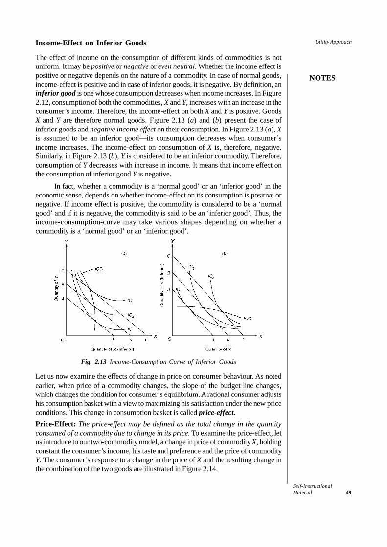
Self-InstructionalMaterial 49
Utility Approach
NOTES
Income-Effect on Inferior Goods
The effect of income on the consumption of different kinds of commodities is notuniform. It may be positive or negative or even neutral. Whether the income effect ispositive or negative depends on the nature of a commodity. In case of normal goods,income-effect is positive and in case of inferior goods, it is negative. By definition, aninferior good is one whose consumption decreases when income increases. In Figure2.12, consumption of both the commodities, X and Y, increases with an increase in theconsumer’s income. Therefore, the income-effect on both X and Y is positive. GoodsX and Y are therefore normal goods. Figure 2.13 (a) and (b) present the case ofinferior goods and negative income effect on their consumption. In Figure 2.13 (a), Xis assumed to be an inferior good—its consumption decreases when consumer’sincome increases. The income-effect on consumption of X is, therefore, negative.Similarly, in Figure 2.13 (b), Y is considered to be an inferior commodity. Therefore,consumption of Y decreases with increase in income. It means that income effect onthe consumption of inferior good Y is negative.
In fact, whether a commodity is a ‘normal good’ or an ‘inferior good’ in theeconomic sense, depends on whether income-effect on its consumption is positive ornegative. If income effect is positive, the commodity is considered to be a ‘normalgood’ and if it is negative, the commodity is said to be an ‘inferior good’. Thus, theincome-consumption-curve may take various shapes depending on whether acommodity is a ‘normal good’ or an ‘inferior good’.
Fig. 2.13 Income-Consumption Curve of Inferior Goods
Let us now examine the effects of change in price on consumer behaviour. As notedearlier, when price of a commodity changes, the slope of the budget line changes,which changes the condition for consumer’s equilibrium. A rational consumer adjustshis consumption basket with a view to maximizing his satisfaction under the new priceconditions. This change in consumption basket is called price-effect.Price-Effect: The price-effect may be defined as the total change in the quantityconsumed of a commodity due to change in its price. To examine the price-effect, letus introduce to our two-commodity model, a change in price of commodity X, holdingconstant the consumer’s income, his taste and preference and the price of commodityY. The consumer’s response to a change in the price of X and the resulting change inthe combination of the two goods are illustrated in Figure 2.14.
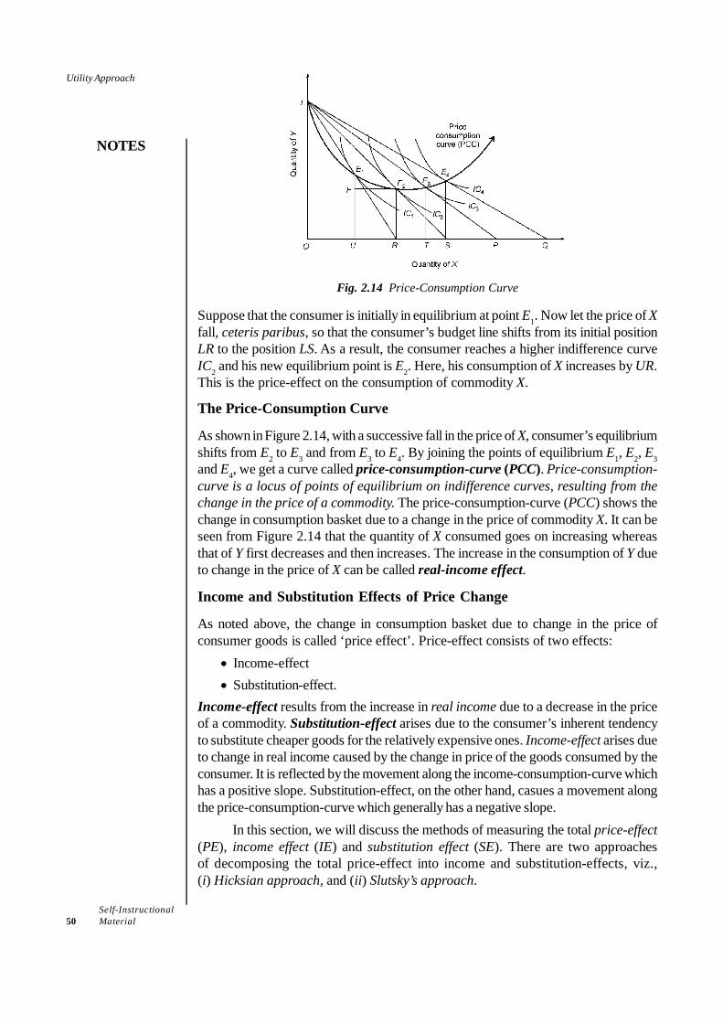
Self-Instructional50 Material
Utility Approach
NOTES
Fig. 2.14 Price-Consumption Curve
Suppose that the consumer is initially in equilibrium at point E1. Now let the price of Xfall, ceteris paribus, so that the consumer’s budget line shifts from its initial positionLR to the position LS. As a result, the consumer reaches a higher indifference curveIC2 and his new equilibrium point is E2. Here, his consumption of X increases by UR.This is the price-effect on the consumption of commodity X.
The Price-Consumption Curve
As shown in Figure 2.14, with a successive fall in the price of X, consumer’s equilibriumshifts from E2 to E3 and from E3 to E4. By joining the points of equilibrium E1, E2, E3and E4, we get a curve called price-consumption-curve (PCC). Price-consumption-curve is a locus of points of equilibrium on indifference curves, resulting from thechange in the price of a commodity. The price-consumption-curve (PCC) shows thechange in consumption basket due to a change in the price of commodity X. It can beseen from Figure 2.14 that the quantity of X consumed goes on increasing whereasthat of Y first decreases and then increases. The increase in the consumption of Y dueto change in the price of X can be called real-income effect.
Income and Substitution Effects of Price Change
As noted above, the change in consumption basket due to change in the price ofconsumer goods is called ‘price effect’. Price-effect consists of two effects:
• Income-effect• Substitution-effect.
Income-effect results from the increase in real income due to a decrease in the priceof a commodity. Substitution-effect arises due to the consumer’s inherent tendencyto substitute cheaper goods for the relatively expensive ones. Income-effect arises dueto change in real income caused by the change in price of the goods consumed by theconsumer. It is reflected by the movement along the income-consumption-curve whichhas a positive slope. Substitution-effect, on the other hand, casues a movement alongthe price-consumption-curve which generally has a negative slope.
In this section, we will discuss the methods of measuring the total price-effect(PE), income effect (IE) and substitution effect (SE). There are two approachesof decomposing the total price-effect into income and substitution-effects, viz.,(i) Hicksian approach, and (ii) Slutsky’s approach.
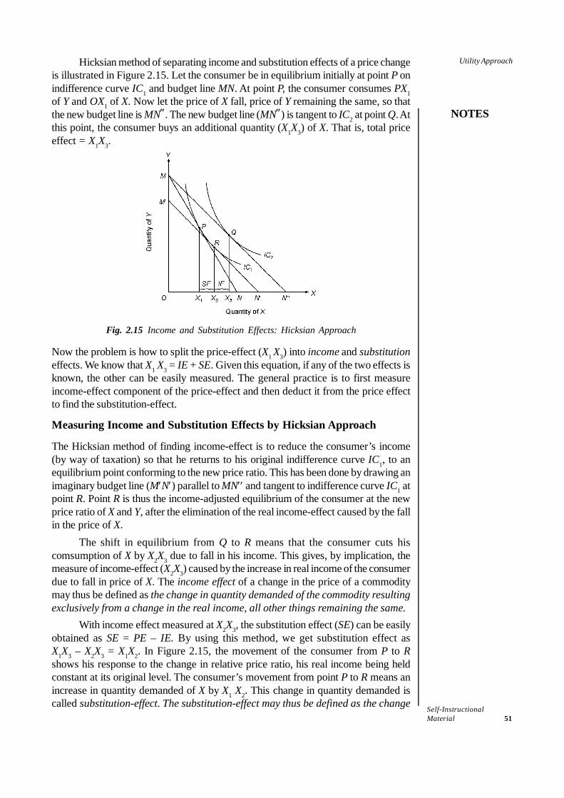
Self-InstructionalMaterial 51
Utility Approach
NOTES
Hicksian method of separating income and substitution effects of a price changeis illustrated in Figure 2.15. Let the consumer be in equilibrium initially at point P onindifference curve IC1 and budget line MN. At point P, the consumer consumes PX1of Y and OX1 of X. Now let the price of X fall, price of Y remaining the same, so thatthe new budget line is MN″. The new budget line (MN″) is tangent to IC2 at point Q. Atthis point, the consumer buys an additional quantity (X1X3) of X. That is, total priceeffect = X1X3.
Fig. 2.15 Income and Substitution Effects: Hicksian Approach
Now the problem is how to split the price-effect (X1 X3) into income and substitutioneffects. We know that X1 X3 = IE + SE. Given this equation, if any of the two effects isknown, the other can be easily measured. The general practice is to first measureincome-effect component of the price-effect and then deduct it from the price effectto find the substitution-effect.
Measuring Income and Substitution Effects by Hicksian Approach
The Hicksian method of finding income-effect is to reduce the consumer’s income(by way of taxation) so that he returns to his original indifference curve IC1, to anequilibrium point conforming to the new price ratio. This has been done by drawing animaginary budget line (M′N′) parallel to MN′′ and tangent to indifference curve IC1 atpoint R. Point R is thus the income-adjusted equilibrium of the consumer at the newprice ratio of X and Y, after the elimination of the real income-effect caused by the fallin the price of X.
The shift in equilibrium from Q to R means that the consumer cuts hiscomsumption of X by X2X3 due to fall in his income. This gives, by implication, themeasure of income-effect (X2X3) caused by the increase in real income of the consumerdue to fall in price of X. The income effect of a change in the price of a commoditymay thus be defined as the change in quantity demanded of the commodity resultingexclusively from a change in the real income, all other things remaining the same.
With income effect measured at X2X3, the substitution effect (SE) can be easilyobtained as SE = PE – IE. By using this method, we get substitution effect asX1X3 – X2X3 = X1X2. In Figure 2.15, the movement of the consumer from P to Rshows his response to the change in relative price ratio, his real income being heldconstant at its original level. The consumer’s movement from point P to R means anincrease in quantity demanded of X by X1 X2. This change in quantity demanded iscalled substitution-effect. The substitution-effect may thus be defined as the change
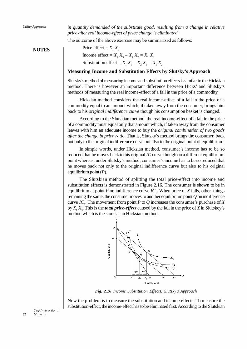
Self-Instructional52 Material
Utility Approach
NOTES
in quantity demanded of the substitute good, resulting from a change in relativeprice after real income-effect of price change is eliminated.The outcome of the above exercise may be summarized as follows:
Price effect = X1 X3
Income effect = X1 X3 – X1 X2 = X2 X3
Substitution effect = X1 X3 – X2 X3 = X1 X2
Measuring Income and Substitution Effects by Slutsky’s Approach
Slutsky’s method of measuring income and substitution effects is similar to the Hicksianmethod. There is however an important difference between Hicks’ and Slutsky’smethods of measuring the real income-effect of a fall in the price of a commodity.
Hicksian method considers the real income-effect of a fall in the price of acommodity equal to an amount which, if taken away from the consumer, brings himback to his original indifference curve though his consumption basket is changed.
According to the Slutskian method, the real income-effect of a fall in the priceof a commodity must equal only that amount which, if taken away from the consumerleaves with him an adequate income to buy the original combination of two goodsafter the change in price ratio. That is, Slutsky’s method brings the consumer, backnot only to the original indifference curve but also to the original point of equilibrium.
In simple words, under Hicksian method, consumer’s income has to be soreduced that he moves back to his original IC curve though on a different equilibriumpoint whereas, under Slutsky’s method, consumer’s income has to be so reduced thathe moves back not only to the original indifference curve but also to his originalequilibrium point (P).
The Slutskian method of splitting the total price-effect into income andsubstitution effects is demonstrated in Figure 2.16. The consumer is shown to be inequilibrium at point P on indifference curve IC1. When price of X falls, other thingsremaining the same, the consumer moves to another equilibrium point Q on indifferencecurve IC3. The movement from point P to Q increases the consumer’s purchase of Xby X1 X3. This is the total price-effect caused by the fall in the price of X in Slutskey’smethod which is the same as in Hicksian method.
Fig. 2.16 Income Substitution Effects: Slutsky’s Approach
Now the problem is to measure the substitution and income effects. To measure thesubstitution-effect, the income-effect has to be eliminated first. According to the Slutskian

Self-InstructionalMaterial 53
Utility Approach
NOTES
approach, a consumer’s real income is so reduced that he is able to purchase hisoriginal combination of the two goods (i.e., OX1 of X and PX1 of Y) at the new priceratio. This is accomplished by drawing an imaginary budget line, M′N′ through thepoint P. Since the whole commodity space is full of indifference curves, one of theindifference curves (IC2) is tangent to the imaginary budget line M′N′ at point R. Themovement from point Q to R shows a fall in the consumption of X by X2 X3. This isSlutskian income effect. We may now easily find out the substitution effect (SE) bysubtracting the income-effect (IE) from the total price-effect (PE), as given below.
Substitution Effect = PE – IE = SE= X1 X3 – X2 X3 = X1 X2
In Figure 2.16, the movement from P to R and the consequent increase in thequantity purchased of X (i.e., X1 X2) is the substitution effect. Similarly, the consumer’smovement from R to Q and the consequent increase in the quantity purchased of X isthe income-effect.
Hicksian Approach Versus Slutskian Approach: Figure 2.17 compares theHicksian and Slutskian approaches of splitting price-effect into substitution and incomeeffects and also their results. The Slutskian approach attempts to hold only apparentreal income constant which is obtained by adjusting consumer’s real income by theamount of ‘cost-difference’ so that the consumer is left with an income just sufficientto buy the original combination of the goods. The Hicksian approach, on the otherhand, holds constant the real income expressed in terms of the original level ofsatisfaction so that the consumer is able to stay on the original indifference curve. Toexpress the difference graphically, Hicksian method puts the consumer on the originalindifference curve whereas Slutskian method makes the consumer move to an upperindifference curve.
Let us compare the two methods in Figure 2.17. Let the consumer be in equilibriumat point P on indifference curve IC1. When the price of X falls the consumer moves topoint Q. The movement from P to Q is the total price-effect which equals X1 X4 ofcommodity X. Upto this point, there is no difference between Slutsky and Hicks.Beyond this point, they differ. According to the Slutskian approach, the movementfrom P to T is the substitution effect and the movement from T to Q is the incomeeffect. According to the Hicksian approach, the movement from P to R is the substitutioneffect and movement from R to Q is the income effect. The substitution and incomeeffects of Slutskian and Hicksian approaches are summed up in quantitative terms inthe following table.
Fig. 2.17 Hicksian Approach vs. Slutskian Approach
Self-Instructional54 Material
Utility Approach
NOTES
Method Price-effect Substitution-effect Income-effect
Hicksian X1X4 X1X2 X2X4
Slutskian X1X4 X1X3 X3X4
As Figure 2.17 shows, there is a good deal of difference between Hicksian and Slustkianmeasures of income and substitution effects. But it can be shown that if the change inprice is small, the difference between the Slutskian and Hicksian measures would besmall and if ΔP tends to be zero, the difference would also be zero.
Apart from the above difference between the two methods, there are someother differences also. While the Hicksian approach is considered as a ‘highly persuasivesolution’ to the problem of splitting price-effect into substitution and income effects,the Slutskian approach is intuitively ‘perhaps less satisfying’.4 But the merit of theSlutskian approach is that substitution and income effects can be directly computedfrom the observed facts, whereas the Hicksian measure of these effects cannot beobtained without the knowledge of a consumer’s indifference map.
Both the methods, have however, their own merits. The merit of the Slutskianmethod, which Hicks calls the ‘cost-difference’ method, lies in its property that itmakes income effect easy to handle. Hicks has himself recognized this merit of theSlutskian method. The merit of Hicksian method or ‘compensating variation method’is that it is a more convenient method of measuring the substitution effect. In Hicks’own words, ‘The merit of the cost-difference method is confined to [its] property...that its income effect is peculiarly easy to handle. The compensating variation method[i.e., his own method] does not share in this particular advantage; but it makes up forits clumsiness in relation to income-effect by its convenience with relation to thesubstitution effect.’5
Predictability of Income and Substitution Effects: Let us now look into the needfor separating the income and substitution effects. As Hicks6 has pointed out,‘substitution effect is absolutely certain; it must always work in favour of an increasein demand for a commodity when the price of that commodity falls.’ Thus, the behaviourof substitution effect is predictable; it follows directly from the principle of diminishingmarginal rate of substitution. On the contrary, “income effect is not so reliable’7 andits behaviour is unpredictable in general. In fact, whether income-effect is positive ornegative depends on whether a commodity is treated by the consumer as a ‘superior’or an ‘inferior’ good. Since the subjective valuation of a commodity may vary fromperson to person, the response of the consumer in general to a change in real incomebecomes uncertain and unpredictable. It is quite likely that in some cases, substitutioneffect works in a positive direction, while income-effect works in a negative direction.In such cases a systematic analysis of price-demand relationship becomes an extremelydifficult task. It becomes necessary, therefore, to eliminate the unpredictable incomeeffect so that the behaviour of the predictable substitution effect can be known. Apartfrom its analytical importance, the knowledge of ‘how powerful is the substitutioneffect’ is essential for formulating an appropriate pricing strategy.
2.3.5 Derivation of Individual Demand Curve
The basic purpose of the entire exercise in indifference curve technique is to constructthe individual demand curve for a commodity. As stated earlier, the individual demandcurve shows the relationship between the quantity demanded of a commodity (say X)by an individual and its price (Px) under the ceteris paribus assumption. Thus, to draw
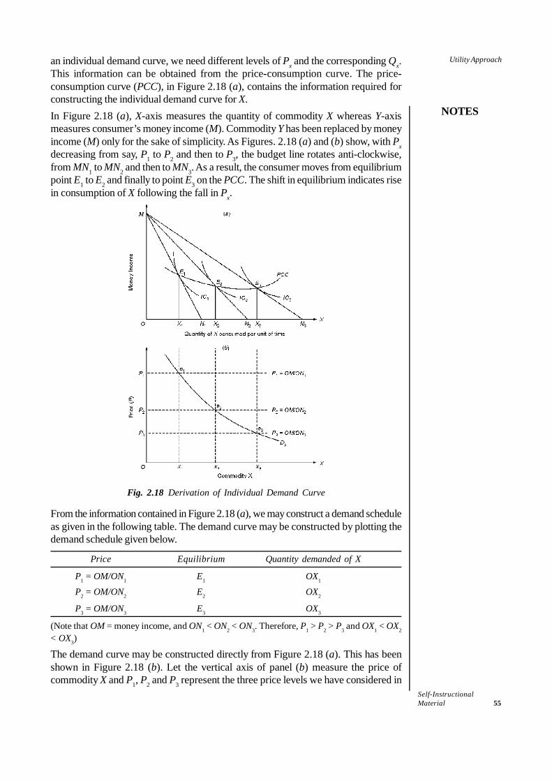
Self-InstructionalMaterial 55
Utility Approach
NOTES
an individual demand curve, we need different levels of Px and the corresponding Qx.This information can be obtained from the price-consumption curve. The price-consumption curve (PCC), in Figure 2.18 (a), contains the information required forconstructing the individual demand curve for X.In Figure 2.18 (a), X-axis measures the quantity of commodity X whereas Y-axismeasures consumer’s money income (M). Commodity Y has been replaced by moneyincome (M) only for the sake of simplicity. As Figures. 2.18 (a) and (b) show, with Pxdecreasing from say, P1 to P2 and then to P3, the budget line rotates anti-clockwise,from MN1 to MN2 and then to MN3. As a result, the consumer moves from equilibriumpoint E1 to E2 and finally to point E3 on the PCC. The shift in equilibrium indicates risein consumption of X following the fall in Px.
Fig. 2.18 Derivation of Individual Demand Curve
From the information contained in Figure 2.18 (a), we may construct a demand scheduleas given in the following table. The demand curve may be constructed by plotting thedemand schedule given below.
Price Equilibrium Quantity demanded of X
P1 = OM/ON1 E1 OX1
P2 = OM/ON2 E2 OX2
P3 = OM/ON3 E3 OX3
(Note that OM = money income, and ON1 < ON2 < ON3. Therefore, P1 > P2 > P3 and OX1 < OX2
< OX3)
The demand curve may be constructed directly from Figure 2.18 (a). This has beenshown in Figure 2.18 (b). Let the vertical axis of panel (b) measure the price ofcommodity X and P1, P2 and P3 represent the three price levels we have considered in

Self-Instructional56 Material
Utility Approach
NOTES
part (a). If we draw horizontal lines from P1, P2, and P3, we get the three price levels inpart (b). We know from panel (a) that at price OM/OX1 (= P1), the quantity consumedis OX1. If we extend the ordinate E1X1 to the X-axis of part (b), it intersects the line P1= OM/ON1 at point e1. By repeating this process for equilibrium points E2 and E3 inFigure 2.18 (a), we get points e2 and e3 in Figure 2.18 (b). By joining the points e1, e2,and e3 we get the demand curve Dx. This demand curve is the same as the Marshalliandemand curve.Possible Shapes of the Demand Curve: The precise shape and slope of a demandcurve derived from indifference curves depends on the direction in which income andsubstitution effects work as a result of fall in the price of a commodity. In fact, thesubstitution effect is always negative but income-effect is uncertain. Therefore, giventhe negative substitution effect, the shape and nature of demand curve depends on thedirection and magnitude of the income-effect. There are four possible combinationsof substitution and income effects for a fall in the commodity price and the correspondingnature of the demand curve. These may be summarized as follows:
1. When substitution-effect is negative and income-effect is positive, quantitydemanded of X increases as Px decreases. The demand curve, therefore, slopesdownward to the right. This is the case with ‘normal goods’.
2. If income-effect is negative but less than the (negative) substitution effect (ashappens in case of inferior goods) the demand curve slopes downward to theright more steeply than usual.
3. If income-effect is zero, the demand curve follows the substitution effect, i.e.,as price decreases, demand increases. The demand curve has a negative slope,but is relatively flatter.
4. If income-effect is negative and more powerful than the substitution-effect (ashappens in the case of Giffen goods) the demand curve becomes backwardbending, as shown in Figure 2.19. But it is most unlikely that any demand curvewill slope downward to the left throughout its whole length.8 It will be so onlyover that range of price changes over which the negative income-effect is strongerthan the substitution-effect. Therefore, the most likely shape of the demandcurve9 for a Giffen good is one shown in Figure 2.19. The demand curve for aGiffen good slopes downward till price falls to P2. But if price falls further, theincome-effect may become negative and so powerful that it outweighs thesubstitution effect. Then the demand curve for a Giffen good becomes abackward sloping one. If price continues to fall, say below P1, the demand mayonce again increase for the Giffen good. This seems to be the most likely shapeof the demand curve for a Giffen good.
Fig. 2.19 Demand Curve for a Giffen Good
Self-InstructionalMaterial 57
Utility Approach
NOTES
2.3.6 Comparison of Cardinal and Ordinal Utility Approaches
Having outlined the indifference curve technique, let us now compare the cardinal andordinal utility approaches to consumer’s analysis and look into the relative merits ofthe two approaches.
Similarity between the two approaches
Some basic assumptions are the same: Some of the assumptions made under thetwo approaches are the same. Both cardinal and ordinal approaches assume rationalityand utility maximizing behaviour of the consumer. The diminishing marginal utilityassumption of the cardinal utility approach is implicit in the diminishing marginalrate of substitution assumption of the ordinal utility approach.Equilibrium conditions are identical: Both cardinal and ordinal utility approachesarrive at an identical equilibrium condition. The necessary (or the first order) equilibriumcondition of the cardinal utility approach, i.e.,
x
y
MUMU = y
x
PP
and the first order (or necessary) equilibrium condition of the ordinal utility approachgiven as are, in fact, one and the same because MUx/MUy = MRSx, y.
MRSx, y = x
y
PP
The second order equilibrium condition of the cardinal utility approach is thatthe total expenditure must not exceed the consumer’s total income. This is similar tothe second order condition of the ordinal utility approach, i.e., the first order equilibriumcondition must be fulfilled at the highest possible indifference curve on his indifferencemap.
Thus, in spite of the fact that cardinal and ordinal approaches are based ondifferent assumptions regarding measurability of utility, both arrive at the sameconclusion with respect to consumer behaviour.
Superiority of Indifference Curve Approach
In spite of their similarity in some respects, indifference curve analysis is in manyrespects superior to the cardinal utility approach. The indifference curve analysis hasmade major advances in the theory of consumer analysis at least in the followingrespects.First, the assumptions of the indifference curve approach are less stringent or restrictivethan those of the cardinal utility approach. While cardinal utility approach assumescardinal measurability of utility, the ordinal approach assumes only ordinal expressionof utility. Besides, unlike the cardinal utility approach, the ordinal utility approach doesnot assume constancy of utility of money. The Marshallian assumption of constancyof marginal utility of money is incompatible with demand functions involving morethan one good.Second, indifference curve approach provides a better criterion for the classificationof goods into substitutes and complements. This is considered as one of the mostimportant contributions of the ordinal utility approach. The cardinal utility approachuses the sign of cross-elasticity for the purpose of classifying goods into substitutesand complements. The cross-elasticity between two goods, X and Y, is given by

Self-Instructional58 Material
Utility Approach
NOTES
ex, y = .y x
x y
Q PP Q
Δ
Δ
If cross-elasticity has a positive sign, it means X and Y are substitutes for each otherand if elasticity has a negative sign, it means they are complements. This method ofclassifying goods into substitutes and compliments is somewhat misleading. For, asshown in the above measure of cross-elasticity, it uses the total effect of a pricechange (ΔPx) on quantity demanded (ΔQy) without compensating for the change inreal income caused by the change in the price of the commodity (i.e., ΔPx). On thecontrary, the indifference curve analysis suggests measuring cross-elasticity aftercompensating for the changes in real income resulting from the change in Px. Accordingto Hicks, goods X and Y are substitutes for each other if cross-elasticity measuredafter eliminating the income effect is positive.
Although the Hicksian criterion for classifying goods into substitutes andcomplements is theoretically superior to the cross-elasticity method (unadjusted forreal income-effect) and provides greater insight into the price-effect, it is impracticable.The reason is estimating income and substitution effects of a price-change is an extremelydifficult task in the absence of an empirial indifference curve. On the other hand, theusual cross-elasticity method is feasible because it requires only the knowledge of themarket demand function which is empirically estimable.Third, indifference curve analysis provides a more realistic measure of consumer’ssurplus compared to one provided by Marshall. The Marshallian concept of‘Consumer’s surplus’ is based on the assumptions that utility is cardinally measurablein terms of money and that utility of money remains constant. Neither of these twoassumptions is realistic. Indifference curve analysis measures consumer’s surplus interms of ordinal utility. The Hicksian measure of consumer’s surplus is of greatimportance in welfare economics and in the formulation and assessment of governmentpolicy.
2.4 SUMMARY
• From the product angle, utility is the want-satisfying property of a commodity.From consumer’s angle, utility is the psychological feeling of satisfaction,pleasure, happiness or well-being, which a consumer derives from theconsumption, possession or the use of a commodity.
• Assuming that utility is measurable and additive, total utility may be defined asthe sum of the utility derived by a consumer from the various units of a good orservice he consumes at a point or over a period of time.
• Marginal utility may be defined in a number of ways. It is defined as the utilityderived from the marginal or one additional unit consumed. It may also bedefined as the addition to the total utility resulting from the consumption (oraccumulation) of one additional unit.
• Based on cardinal and ordinal concepts of utility, there are two approaches tothe analysis of consumer behaviour.o Cardinal Utility approach, attributed to Alfred Marshall and his followers, is
also called the Neo-classical Approach.o Ordinal Utility approach, pioneered by J.R. Hicks, a Nobel laureate, and
R.G.D. Allen, is also called the Indifference Curve Analysis.
Check Your Progress
3. State the law ofdiminishing marginalutility.
4. State the twoapproaches to theanalysis ofconsumer behaviour.
5. Define anindifference curve.
6. What is priceeffect?
7. Define an income-consumption curve.
8. What is an inferiorgood?
Self-InstructionalMaterial 59
Utility Approach
NOTES
• Conceptually, a consumer reaches his equilibrium position when he has maximizedthe level of his satisfaction, given his resources and other conditions. Technically,a utility-maximizing consumer reaches his equilibrium position when allocation ofhis expenditure is such that the last penny spent on each commodity yields thesame utility.
• An indifference curve may be defined as the locus of points each representing adifferent combination of two substitute goods, which yield the same utility orlevel of satisfaction to the consumer.
• The MRS is the rate at which one commodity can be substituted for another,the level of satisfaction remaining the same.
• The MRS diminishes along the IC curve because, in most cases, no two goodsare perfect substitutes for one another. In case any two goods are perfectsubstitutes, the indifference curve will be a straight line having a negative slopeshowing constant MRS. Since goods are not perfect substitutes, the subjectivevalue attached to the additional quantity (i.e., subjective MU) of a commoditydecreases fast in relation to the other commodity whose total quantity isdecreasing.
• Indifference curves have the following four basic properties:o Indifference curves have a negative slopeo Indifference curves of imperfect substitutes are convex to the origino Indifference curves do not intersect nor are they tangent to one anothero Upper indifference curves indicate a higher level of satisfaction
• The income-consumption curve may be defined as the locus of points representingvarious equilibrium quantities of two commodities consumed by a consumer atdifferent levels of income, all other things remaining constant.
• The price-effect may be defined as the total change in the quantity consumed ofa commodity due to change in its price.
• Price-consumption-curve is a locus of points of equilibrium on indifferencecurves, resulting from the change in the price of a commodity.
• Income-effect results from the increase in real income due to a decrease in theprice of a commodity. Substitution-effect arises due to the consumer’s inherenttendency to substitute cheaper goods for the relatively expensive ones.
• Both cardinal and ordinal approaches assume rationality and utility maximizingbehaviour of the consumer.
• Both cardinal and ordinal utility approaches arrive at an identical equilibriumcondition.
• In spite of their similarity in some respects, indifference curve analysis is inmany respects superior to the cardinal utility approach.
2.5 KEY TERMS
• Utility: Utility is the psychological feeling of satisfaction, pleasure, happinessor well-being, which a consumer derives from the consumption, possession orthe use of a commodity.
• Total utility: Assuming that utility is measurable and additive, total utility maybe defined as the sum of the utility derived by a consumer from the variousunits of a good or service he consumes at a point or over a period of time.

Self-Instructional60 Material
Utility Approach
NOTES
• Marginal utility: It is defined as the utility derived from the marginal or oneadditional unit consumed.
• Indifference curve: An indifference curve may be defined as the locus of pointseach representing a different combination of two substitute goods, which yieldthe same utility or level of satisfaction to the consumer.
• Income consumption curve: The income-consumption curve may be definedas the locus of points representing various equilibrium quantities of twocommodities consumed by a consumer at different levels of income, all otherthings remaining constant.
• Price-consumption-curve: It is a locus of points of equilibrium on indifferencecurves, resulting from the change in the price of a commodity.
• Price effect: The price-effect may be defined as the total change in the quantityconsumed of a commodity due to change in its price.
2.6 ANSWERS TO ‘CHECK YOUR PROGRESS’
1. Assuming that utility is measurable and additive, total utility may be defined asthe sum of the utility derived by a consumer from the various units of a good orservice he consumes at a point or over a period of time.
2. Marginal utility is defined as the utility derived from the marginal or one additionalunit consumed. It may also be defined as the addition to the total utility resultingfrom the consumption (or accumulation) of one additional unit.
3. The law of diminishing marginal utility states that as the quantity consumed of acommodity goes on increasing, the utility derived from each successive unitgoes on diminishing, consumption of all other commodities remaining the same.
4. There are two approaches to the analysis of consumer behaviour:• Cardinal Utility approach, attributed to Alfred Marshall and his followers, is
also called the Neo-classical Approach.• Ordinal Utility approach, pioneered by J.R. Hicks, a Nobel laureate, and
R.G.D. Allen, is also called the Indifference Curve Analysis.5. An indifference curve may be defined as the locus of points each representing a
different combination of two substitute goods, which yield the same utility orlevel of satisfaction to the consumer.
6. The price-effect may be defined as the total change in the quantity consumed ofa commodity due to change in its price.
7. The income-consumption curve may be defined as the locus of points representingvarious equilibrium quantities of two commodities consumed by a consumer atdifferent levels of income, all other things remaining constant.
8. An inferior good is one whose consumption decreases when income increases.

Self-InstructionalMaterial 61
Utility Approach
NOTES
2.7 QUESTIONS AND EXERCISES
Short-Answer Questions
1. List the assumptions of law of diminishing marginal utility.2. Why does the marginal rate of substitution (MRS) go on decreasing?3. State the assumptions of ordinal utility theory.4. Write a short note on the shift in the budget line.5. Distinguish between income effect and substitution effect.
Long-Answer Questions
1. Analyse consumer’s behaviour using cardinal utility approach.2. Discuss the properties of indifference curve with the help of illustrations.3. Distinguish between cardinal and ordinal utility approaches.4. Discuss the Hicksian and Slustsky’s approach of measuring income and
substitution effects. Compare the Hicksian and Slustkian approach.5. Why is the indifference curve analysis considered to be superior to the cardinal
utility approach?
2.8 FURTHER READING/ENDNOTES
Varshney and Maheshwari. 2011. Managerial Economics. New Delhi: Sultan Chandand Sons.
Mankar, V. G. 1982. Business Economics. New Delhi: Himalya Publishing House.Dufty, N.F. 1966. Managerial Economics. New York: Asia Publishing House.
Endnotes
1. The utility of money income can be viewed in terms of its purchasing power, liquidity,asset function, social prestige, etc. However, in Marshallian analysis, utility of moneyis assumed to remain constant and one unit of money equals one util.
2. Marshall, Alfred, Principles of Economics, Mathematical Appendix II.3. Value and Capital, 1956, p. 13.4. Baumol, W.J., Economic Theory and Operations Analysis, Fourth Edition, New
Delhi.5. Hicks, J.R. A Revision of Demand Theory, (Oxford, 1969), p. 69.6. Hicks, J.R. Value and Capital p. 32.7. Hicks, J.R. Value and Capital, p. 32.8. Stonier A.W. and D.C. Hague, A Textbook of Economic Theory, (London, Longman,
1972), p. 71.9. Stonier and Hague, op. cit., p. 71.


Self-InstructionalMaterial 63
Demand Analysis andForecasting
NOTES
UNIT 3 DEMAND ANALYSIS ANDFORECASTING
Structure3.0 Introduction3.1 Unit Objectives3.2 Demand Schedule and Demand Curve3.3 Significance of Demand Forecasting and Techniques
3.3.1 Steps in Demand Forecasting3.3.2 Techniques of Demand Forecasting
3.4 Some Case Studies of Demand Forecasting3.5 Summary3.6 Key Terms3.7 Answers to ‘Check Your Progress’3.8 Questions and Exercises3.9 Further Reading/Endnotes
3.0 INTRODUCTION
The working of the market system is governed by certain fundamental laws of marketcalled the laws of demand and supply. The laws of demand and supply play a crucialrole in determining the price of a commodity and the size of the market. The theory ofdemand deals with current demand whereas a major concern of businessmen, especiallythe big one, is ‘what would be the future demand for their product?’ This questionarises because the knowledge about future demand for the firm’s product helps inforward planning of production, acquiring inputs (man, material and capital), managingfinances and chalking out future pricing strategy. For this purpose, businessmen maketheir own estimates or even a ‘guesstimate’ of the future demand for their product ortake the help of specialized consultants or market research agencies to get the demandfor their product forecast. In this unit, we will discuss the various methods of demandforecasting and their advantages and limitations.
3.1 UNIT OBJECTIVES
After going through this unit, you will be able to:• Explain a demand schedule and demand curve• Discuss the significance and techniques of demand forecasting
3.2 DEMAND SCHEDULE AND DEMAND CURVE
The demand side of the market for a product refers to all its consumers and the pricethat they are willing to pay for buying a certain quantity of the product during a periodof time. The quantity that consumers buy at a given price determines the market size.It is the size of the market that determines the business prospects of a firm and anindustry. The demand side of the market is governed by the Law of Demand. The law
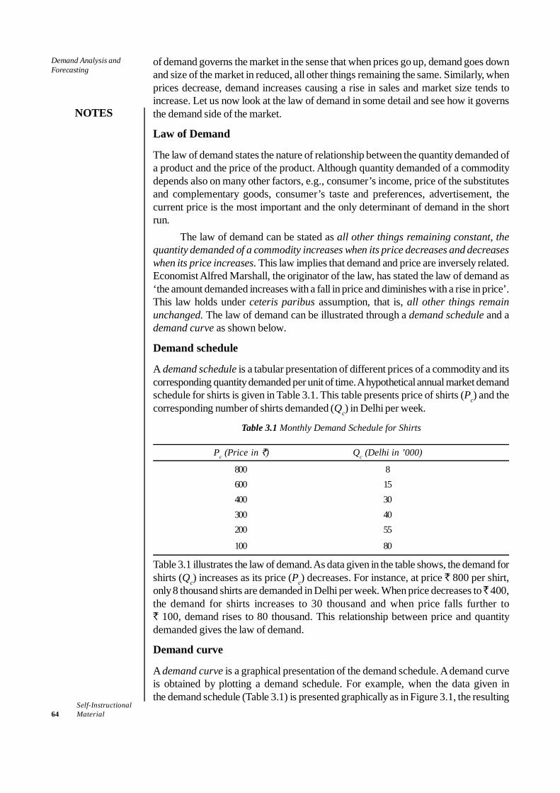
Self-Instructional64 Material
Demand Analysis andForecasting
NOTES
of demand governs the market in the sense that when prices go up, demand goes downand size of the market in reduced, all other things remaining the same. Similarly, whenprices decrease, demand increases causing a rise in sales and market size tends toincrease. Let us now look at the law of demand in some detail and see how it governsthe demand side of the market.
Law of Demand
The law of demand states the nature of relationship between the quantity demanded ofa product and the price of the product. Although quantity demanded of a commoditydepends also on many other factors, e.g., consumer’s income, price of the substitutesand complementary goods, consumer’s taste and preferences, advertisement, thecurrent price is the most important and the only determinant of demand in the shortrun.
The law of demand can be stated as all other things remaining constant, thequantity demanded of a commodity increases when its price decreases and decreaseswhen its price increases. This law implies that demand and price are inversely related.Economist Alfred Marshall, the originator of the law, has stated the law of demand as‘the amount demanded increases with a fall in price and diminishes with a rise in price’.This law holds under ceteris paribus assumption, that is, all other things remainunchanged. The law of demand can be illustrated through a demand schedule and ademand curve as shown below.
Demand schedule
A demand schedule is a tabular presentation of different prices of a commodity and itscorresponding quantity demanded per unit of time. A hypothetical annual market demandschedule for shirts is given in Table 3.1. This table presents price of shirts (Pc) and thecorresponding number of shirts demanded (Qc) in Delhi per week.
Table 3.1 Monthly Demand Schedule for Shirts
Pc (Price in `) Qc (Delhi in ’000)
800 8600 15400 30300 40200 55
100 80
Table 3.1 illustrates the law of demand. As data given in the table shows, the demand forshirts (Qc) increases as its price (Pc) decreases. For instance, at price ` 800 per shirt,only 8 thousand shirts are demanded in Delhi per week. When price decreases to ̀ 400,the demand for shirts increases to 30 thousand and when price falls further to` 100, demand rises to 80 thousand. This relationship between price and quantitydemanded gives the law of demand.
Demand curve
A demand curve is a graphical presentation of the demand schedule. A demand curveis obtained by plotting a demand schedule. For example, when the data given inthe demand schedule (Table 3.1) is presented graphically as in Figure 3.1, the resulting
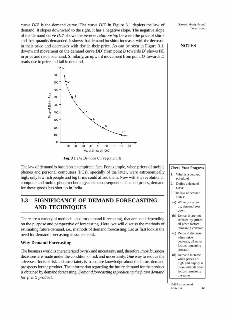
Self-InstructionalMaterial 65
Demand Analysis andForecasting
NOTES
curve DD′ is the demand curve. The curve DD′ in Figure 3.1 depicts the law ofdemand. It slopes downward to the right. It has a negative slope. The negative slopeof the demand curve DD′ shows the inverse relationship between the price of shirtsand their quantity demanded. It shows that demand for shirts increases with the decreasein their price and decreases with rise in their price. As can be seen in Figure 3.1,downward movement on the demand curve DD′ from point D towards D′ shows fallin price and rise in demand. Similarly, an upward movement from point D′ towards Dreads rise in price and fall in demand.
Fig. 3.1 The Demand Curve for Shirts
The law of demand is based on an empirical fact. For example, when prices of mobilephones and personal computers (PCs), specially of the latter, were astronomicallyhigh, only few rich people and big firms could afford them. Now with the revolution incomputer and mobile phone technology and the consequent fall in their prices, demandfor these goods has shot up in India.
3.3 SIGNIFICANCE OF DEMAND FORECASTINGAND TECHNIQUES
There are a variety of methods used for demand forecasting, that are used dependingon the purpose and perspective of forecasting. Here, we will discuss the methods ofestimating future demand, i.e., methods of demand forecasting. Let us first look at theneed for demand forecasting in some detail.
Why Demand Forecasting
The business world is characterized by risk and uncertainty and, therefore, most businessdecisions are made under the condition of risk and uncertainty. One way to reduce theadverse effects of risk and uncertainty is to acquire knowledge about the future demandprospects for the product. The information regarding the future demand for the productis obtained by demand forecasting. Demand forecasting is predicting the future demandfor firm’s product.
Check Your Progress
1. What is a demandschedule?
2. Define a demandcurve.
3. The law of demandstates:
(a) When prices goup, demand goesdown
(b) Demands are notaffected by prices,all other factorsremaining constant
(c) Demand decreasewhen pricedecrease, all otherfactors remainingconstant
(d) Demand increasewhen prices arehigh and supply ismore with all otherfactors remainingthe same

Self-Instructional66 Material
Demand Analysis andForecasting
NOTES
The knowledge about the future demand for the product helps a great deal in the followingareas of business decision-making:
• Planning and scheduling production• Acquiring inputs (labour, raw material and capital)• Making provision for finances• Formulating pricing strategy• Planning advertisement
Demand forecasting assumes greater significance where large-scale production isinvolved. Large-scale production requires a good deal of forward planning as it involvesa long gestation period. The information regarding future demand is also essential forthe existing firms to be able to avoid under or over-production. Most firms are, in fact,very often confronted with the question as to what would be the future demand fortheir products because they will have to acquire inputs and plan their productionaccordingly. The firms are, hence, required to estimate the future demand for theirproducts. Otherwise, their functioning will be shrouded with uncertainty and theirobjective may be defeated.
This problem may not be of a serious nature for small firms which supply a verysmall fraction of the total demand, and whose product caters to the short-term orseasonal demand or the demand of a routine nature. Their past experience and businessskills may be sufficient for the purpose of planning and production. But, firms workingon a large scale find it extremely difficult to obtain a fairly accurate estimate of futuremarket demand.1 In some situations, it is very difficult to obtain information needed tomake even short-term demand forecasts and thus it is extremely difficult to make long-term forecasts. Under such conditions, it is not possible for the firm to determine howchanges in specific demand variables like price, advertisement expenditure, credit terms,prices of competing products, will affect demand. It is nevertheless indispensable forthe large firms to have at least an approximate estimate of the demand prospects. For,demand forecast plays an important role in planning the acquiring of inputs, both menand material (raw material and capital goods), organizing production, advertising theproduct, and organizing sales channels. These functions can hardly be performedsatisfactorily in an atmosphere of uncertainty regarding demand prospects for theproduct. The prior knowledge of market-size, therefore, becomes an essential elementof decision-making by the large-scale firms.
3.3.1 Steps in Demand Forecasting
The objective of demand forecasting is achieved only when forecast is madesystematically and scientifically and when it is fairly reliable. The following steps aregenerally taken to make systematic demand forecasting.
(i) Specifying the objective: The objective or the purpose of demand forecastingmust be clearly specified. The objective may be specified in terms of (a) short-term or long-term demand, (b) the overall demand for a product or for firm’sown product, (c) the whole or only a segment2 of the market for its product, or(d) firm’s market share. The objective of demand forecasting must be determinedbefore the process of forecast is started. This has to be the first step.
(ii) Determining time perspective: Depending on the firm’s objective, demandmay be forecast for a short period, i.e., for the next 2-3 years, or for a longperiod. In demand forecasting for a short period – 2-3 years – many of the
Self-InstructionalMaterial 67
Demand Analysis andForecasting
NOTES
demand determinants can be taken to remain constant or not to change significantly.In the long run, however, demand determinants may change significantly.Therefore, the time perspective of demand forecasting must be specified.
(iii) Making choice of method for demand forecasting: As we will see below, anumber of different demand forecasting methods are available. However, allmethods are not suitable for all kinds of demand forecasting because the purposeof forecasting, data requirement of a method, availability of data and timeframe of forecasting vary from method to method. The demand forecaster has,therefore, to choose a suitable method keeping in view his purpose andrequirements. The choice of a forecasting method is generally based on thepurpose, experience and expertise of the forecaster. It depends also to a greatextent on the availability of required data. The choice of a suitable methodsaves not only time and cost but also ensures the reliability of forecast to a greatextent.
(iv) Collection of data and data adjustment: Once method of demand forecastingis decided on, the next step is to collect the required data—primary or secondaryor both. The required data is often not available in the required mode. In thatcase, data needs to be adjusted—even massaged, if necessary—with the purposeof building data series consistent with data requirement. Sometimes the requireddata has to be generated from the secondary sources.
(v) Estimation and interpretation of results: As mentioned above, the availabilityof data often determines the method, and also the trend equation to be used fordemand forecasting. Once required data is collected and forecasting method isfinalized, the final step in demand forecasting is to make the estimate of demandfor the predetermined years or the period. Where estimates appear in the formof an equation, the result must be interpreted and presented in a usable form.
3.3.2 Techniques of Demand Forecasting
The various techniques of demand forecasting are listed in the chart. In this section,we have explained the various demand forecasting methods and their limitations.
1. Survey methods
Survey methods are generally used where the purpose is to make short-run forecast ofdemand. Under this method, consumer surveys are conducted to collect informationabout their intentions and future purchase plans. This method includes:
• Survey of potential consumers’ plan• Opinion poll of experts.
Let us now discuss the two methods of survey and look at their limitations.(a) Consumer survey method—direct interviews: The consumer survey method
of demand forecasting involves direct interview of the potential consumers.Consumers can be interviewed by any of the following methods, depending onthe purpose, time and cost of survey:• Complete enumeration• Sample survey• End-use methodThese consumer survey methods are used under different conditions and fordifferent purposes. Their advantages and disadvantages are described below.

Self-Instructional68 Material
Demand Analysis andForecasting
NOTES
The most direct and simple way of assessing future demand for a product is tointerview the potential consumers or users and to ask them what quantity of theproduct under reference they would be willing to buy at different prices over agiven period, say, one year. This method is known as direct interview method.This method may cover almost all the potential consumers or only selectedgroups of consumers from different cities or parts of the area of consumerconcentration. When all the consumers are interviewed, the method is known ascomplete enumeration survey or comprehensive interview method and whenonly a few selected representative consumers are interviewed, it is known assample survey method. In the case of industrial inputs, interviews or postalinquiry of only end-users of a product may be required. Let us now describethese methods in detail.
(i) Complete enumeration method: In this method, almost all potential usersof the product are contacted and are asked about their future plan ofpurchasing the product in question. The quantities indicated by theconsumers are added together to obtain the probable demand for theproduct. For example, if majority of households in a city report the quantity(q) they are willing to purchase of a commodity, then total probable demand(Dp) may be calculated as
Dp = q1 + q2 + q3 + …+ qn = ∑=
n
iiq
1
where q1, q2, q3 etc. denote demand by the individual households 1, 2, 3.This method has certain limitations. It can be used successfully only incase of those products whose consumers are concentrated in a certainregion or locality. In case of a widely dispersed market, this method maynot be physically possible or may prove very costly in terms of bothmoney and time. Besides, the demand forecast through this method maynot be reliable for the following reasons.• Consumers themselves may not know their actual demand in future
and hence may be unable or unwilling to answer the query• Even if they answer, their answers to hypothetical questions may be
hypothetical—not real• Consumers’ response may be biased according to their own
expectations about the market conditions• Their plans may change with a change in the factors not included in
the questionnaire(ii) Sample survey method: Sample survey method is used when population
of the target market is very large. Under sample survey method, only asample of potential consumers or users is selected for interview. Consumersto be surveyed are selected from the relevant market through a samplingmethod. Method of survey may be direct interview or mailed questionnaireto the sample-consumers. On the basis of the information obtained, theprobable demand may be estimated through the following formula.
Dp = R
S
HH (H . AD)
where Dp = probable demand forecast; H = census number of householdsfrom the relevant market; Hs = number of households surveyed or sample
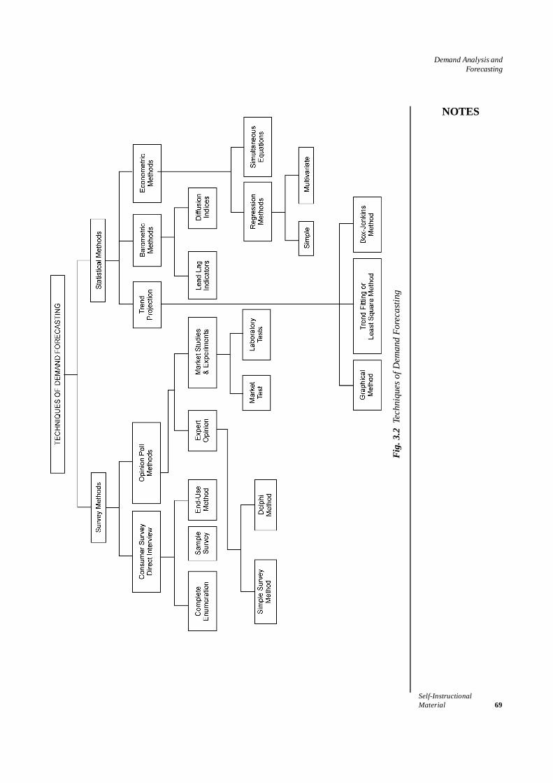
Self-InstructionalMaterial 69
Demand Analysis andForecasting
NOTES
Fig.
3.2
Tech
niqu
es o
f Dem
and
Fore
cast
ing

Self-Instructional70 Material
Demand Analysis andForecasting
NOTES
households; HR = number of households reporting demand for the product;AD = average expected consumption by the reporting households (= totalquantity reported to be consumed by the reporting households ÷ numbersof households).This method is simpler, less costly and less time-consuming compared to thecomprehensive survey method. This method is generally used to estimateshort-term demand of business firms, government departments and agenciesand also of the households who plan their future purchases. Business firms,government departments and other such organizations budget theirexpenditure at least one year in advance. It is, therefore, possible for themto supply a fairly reliable estimate of their future purchases. Even thehouseholds making annual or periodic budgets of their expenditure canprovide reliable information about their purchases.The sample survey method is the most widely used survey method to forecastdemand. This method, however, has some limitations similar to those ofcomplete enumerations or exhaustive survey method. The forecaster,therefore, should not attribute more reliability to the forecast than iswarranted. Besides, the sample survey method can be used to verify thedemand forecast made by using quantitative or statistical methods. Althoughsome authors3 suggest that this method should be used to supplement thequantitative method for forecasting rather than to replace it, this methodcan be gainfully used where the market is localized. Sample survey methodcan be of greater use in forecasting where quantification of variables (e.g.,feelings, opinion, expectations is not possible and where consumer’s behaviouris subject to frequent changes.
(iii) End-use method: The end-use method of demand forecasting has aconsiderable theoretical and practical value, especially in forecastingdemand for inputs. Making forecasts by this method requires building upa schedule of probable aggregate future demand for inputs by consumingindustries and various other sectors. In this method, technological, structuraland other changes that might influence the demand, are taken into accountin the very process of estimation. This aspect of the end-use approach isof particular importance.Stages in the End-use method: The end-use method of demandforecasting consists of four distinct stages of estimation.In the first stage, it is necessary to identify and list all the possible users ofthe product in question. This is, of course, a difficult process, but it isfundamental to this method of forecasting. Difficulty arises becausepublished data on the end-users is rarely available. Despatch records ofthe manufacturers, even if available, need not necessarily provide the numberof all the final users. Records of the sales pattern by individual firms orestablishments are difficult to be assembled. In several cases, sales channelof the products covers such a wide network and there are so many wholesaleand retail agencies in the chain, that it would be virtually impossible toorganize and collect data from all these sources so as to know all the end-uses of the product.Where relevant and adequate data is not available, the managers need tohave a thorough knowledge of the product and its uses. Such knowledgeand experience need to be supplemented by consultations and discussions

Self-InstructionalMaterial 71
Demand Analysis andForecasting
NOTES
with manufacturers or their associations, traders, users, etc. Preparation ofan exhaustive list of all possible end-users is, in any case, a necessary step.Despite every effort made to trace all the end-users, it is quite likely thatsome of the current users of the product are overlooked. In order to accountfor such lapses, it may be necessary at the final stage of estimation toprovide some margin for error. A margin or allowance is also necessary toprovide for possible new applications of the product in the future.The second stage of this method involves fixing suitable technical ‘norms’of consumption of the product under study. Norms have to be establishedfor each and every end-use. Norms are usually expressed in physical termseither per unit of production of the complete product or in, some cases,per unit of investment or per capita use. Sometimes, the norms may involvesocial, moral and ethical values, e.g., in case of consumption of drugs,alcohol or running a dance bar. But value-based norms should be avoidedas far as possible because it might be rather difficult to specify later thetypes and sizes of the product in question if value norms are used.The establishment of norms is also a difficult process mainly due to lackof data. For collecting necessary data, the questionnaire method is generallyemployed. The preparation of a suitable questionnaire is of vital importancein the end-use method, as the entire subsequent analysis has to be basedon and conclusions to flow mainly from the information collected throughthe questionnaires. Where estimating future demand is called for in greatdetail, such as the types and sizes of the concerned product, framing ofthe questionnaire requires a good knowledge of all the variations of theproduct. For a reliable forecast, it is necessary that response is total; ifnot, then as high as possible.Having established the technical norms of consumption for the differentindustries and other end-uses of the product, the third stage is theapplication of the norms. For this purpose, it is necessary to know thedesired or targeted levels of output of the individual industries for thereference year and also the likely development in other economic activitiesthat use the product and the likely output targets.The fourth and final stage in the end-use method is to aggregate theproduct-wise or use-wise content of the item for which the demand is tobe forecast. This aggregate result gives the estimate of demand for theproduct as a whole for the terminal year in question. By the very nature ofthe process of estimation described here, it is obvious that the end-useapproach results in what may be termed as a ‘derived’ demand.Advantages: The end-use method has two exclusive advantages.First, it is possible to work out the future demand for an industrial productin considerable details by types and size. In other methods, the futuredemand can be estimated only at the aggregate level. This is because pastdata are seldom available in such details as to provide the types and sizesof the product demanded by the economy. Hence, projections made byusing the past data, either by the trend method, regression techniques orby historical analogies produce only aggregate figures for the product inquestion. On the other hand, by probing into the present use-pattern ofconsumption of the product, the end-use approach provides every opportunityto determine the types, categories and sizes likely to be demanded in future.
Self-Instructional72 Material
Demand Analysis andForecasting
NOTES
Second, in forecasting demand by the end-use approach, it is possible totrace and pinpoint at any time in future as to where and why the actualconsumption has deviated from the estimated demand. Besides, suitablerevisions can also be made from time to time based on such examination.If projections are based on other methods and if actual consumption fallsbelow or rises above the estimated demand, all that one can say is that theeconomy has or has not picked up as anticipated. One cannot say exactlywhich use of the product has not picked up and why. In the case of end-use method, however, one can.
(b) Opinion poll methods: The opinion poll methods aim at collecting opinions ofthose who are supposed to possess knowledge of the market, e.g., salesrepresentatives, sales executives, professional marketing experts and consultants.The opinion poll methods include:• Expert-opinion method• Delphi method• Market studies and experiments
(i) Expert-opinion method: Firms having a good network of salesrepresentatives can put them on to the work of assessing the demand forthe target product in the areas, regions or cities that they represent. Salesrepresentatives, being in close touch with the consumers or users of goods,are supposed to know the future purchase plans of their customers, theirreactions to the market changes, their response to the introduction of anew product, and the demand for competing products. They are, therefore,in a position to provide at least an approximate, if not accurate, estimateof likely demand for their firm’s product in their region or area. The estimatesof demand thus obtained from different regions are added up to get theoverall probable demand for a product. Firms not having this facility,gather similar information about the demand for their products throughthe professional market experts or consultants, who can predict the futuredemand by using their experience and expertise. This method is also knownas opinion poll method.Limitations: Although this method too is simple and inexpensive, it hasits own limitations.First, estimates provided by the sales representatives or professionalexperts are reliable only to an extent depending on their skill and expertiseto analyze the market and their experience.Secondly, demand estimates may involve the subjective judgement of theassessor which may lead to over or under-estimation.Finally, the assessment of market demand is usually based on inadequateinformation available to the sales representatives as they have only a narrowview of the market. The factors of wider implication, such as change inGNP, availability of credit, future prospects of the industry, etc., fall outsidetheir purview.
(ii) Delphi method:4 Delphi method of demand forecasting is an extension ofthe simple expert opinion poll method. This method is used to consolidatethe divergent expert opinions and to arrive at a compromise estimate offuture demand. The process is simple.Under the Delphi method, the experts are provided information on estimatesof forecasts of other experts along with the underlying assumptions. The
Self-InstructionalMaterial 73
Demand Analysis andForecasting
NOTES
experts may revise their own estimates in the light of forecasts made byother experts. The consensus of experts about the forecasts constitutesthe final forecast. It may be noted that the empirical studies conducted inthe USA have shown that unstructured opinions of the experts is the mostwidely used forecast technique. This may appear a bit unusual in as muchas this gives the impression that sophisticated techniques, e.g., simultaneousequations model and statistical methods, are not the techniques which areused most often. However, the unstructured opinions of the experts mayconceal the fact that information used by experts in expressing theirforecasts may be based on sophisticated techniques. The Delphi techniquecan be used for cross-checking information on forecasts.
(iii) Market studies and experiments: An alternative method of collectingnecessary information regarding current and also future demand for aproduct is to carry out market studies and experiments on consumer’sbehaviour under actual, though controlled, market conditions. This methodis known in common parlance as market experiment method. Under thismethod, firms first select some areas of the representative markets—threeor four cities having similar features, viz., population, income levels, culturaland social background, occupational distribution, choices and preferencesof consumers. Then, they carry out market experiments by changing prices,advertisement expenditure and other controllable variables in the demandfunction under the assumption that other things remain the same. Thecontrolled variables may be changed over time either simultaneously in allthe markets or in the selected markets.5 After such changes are introducedin the market, the consequent changes in the demand over a period of time(a week, a fortnight, or a month) are recorded. On the basis of data collected,elasticity coefficients are computed. These coefficients are then used alongwith the variables of the demand function to assess the future demand forthe product.Alternatively, market experiments can be replaced by consumer clinics orcontrolled laboratory experiments. Under this method, consumers aregiven some money to buy in a stipulated store goods with varying prices,packages, displays. The experiment reveals the consumers’ responsivenessto the changes made in prices, packages and displays, etc. Thus, thelaboratory experiments also yield the same information as the marketexperiments. But the former has an advantage over the latter because ofgreater control over extraneous factors and its somewhat lower cost.Limitations: The market experiment methods have certain seriouslimitations and disadvantages that reduce the usability and reliability ofthis method.First, a very important limitation of the experimental methods is that theyare very expensive. Therefore, experimental methods cannot be affordedby small firms.Secondly, being a costly affair, experiment are usually carried out on ascale too small to permit generalization with a high degree of reliability.Thirdly, experimental methods are based on short-term and controlledconditions which may not exist in an uncontrolled market. Hence the resultsmay not be applicable to the uncontrolled long-term conditions of the market.Fourthly, changes in socio-economic conditions during the field experiments,
Self-Instructional74 Material
Demand Analysis andForecasting
NOTES
such as local strikes or lay-offs, aggressive advertising by competitors, politicalchanges, natural calamities may invalidate the results.Finally, a big disadvantage of experimental methods is that ‘tinkering withprice increases may cause a permanent loss of customers to competitivebrands that might have been tried.’6
Despite these limitations, however, the market experiment method is oftenused to provide an alternative estimate of demand and also ‘as a check onresults obtained from statistical studies.’ Besides, this method generateselasticity co-efficients that are necessary for statistical analysis of demandrelationships. For example, an experiment of this kind was conducted bySimmons Mattress Company (US). It put on sale two types of identicalmattresses—one with Simmons label and the other with an unknown nameat the same price and then at different prices for determining the cross-elasticity. It was found that at the same price, Simmons mattress sold 15to 1; and at a price higher by 5 dollars it sold 8 to 1, and at a price higherby 25 per cent, it sold almost 1 to 1.7
2. Statistical Methods
In the foregoing sections, we have described survey and experimental methods ofestimating demand for a product on the basis of information supplied by the consumersthemselves and on-the-spot observation of consumer behaviour. In this section, wewill explain statistical methods which utilize historical (time-series) and cross-sectionaldata for estimating long-term demand. Statistical methods are considered to be superiortechniques of demand estimation for the following reasons.
• In the statistical methods, the element of subjectivity is minimum• Method of estimation is scientific as it is based on the theoretical relationship
between the dependent and independent variables• Estimates are relatively more reliable• Estimation involves smaller cost
Three kinds of statistical methods are used for demand projection.• Trend projection methods• Barometric methods• Econometric method
These statistical methods are described here briefly.(i) Trend projection methods: Trend projection method is a ‘classical method’ of
business forecasting. This method is essentially concerned with the study ofmovement of variables through time. The use of this method requires a long andreliable time-series data. The trend projection method is used under the assumptionthat the factors responsible for the past trends in the variable to be projected(e.g., sales and demand) will continue to play their part in future in the samemanner and to the same extent as they did in the past in determining the magnitudeand direction of the variable. This assumption may be quite justified in manycases.However, since cause-and-effect relationship is not revealed by this method,the projections made on the trend basis are considered by many as a mechanicalor a ‘naïve’ approach. Nevertheless, ‘There is nothing uncomplimentary in the
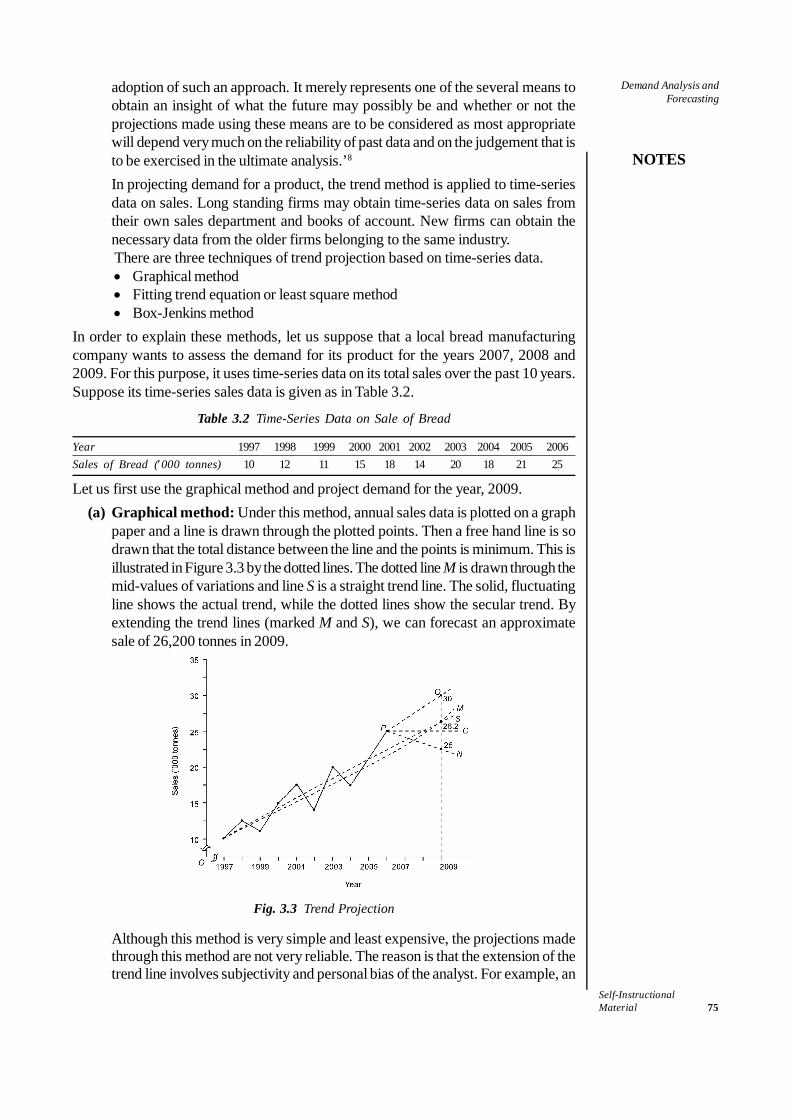
Self-InstructionalMaterial 75
Demand Analysis andForecasting
NOTES
adoption of such an approach. It merely represents one of the several means toobtain an insight of what the future may possibly be and whether or not theprojections made using these means are to be considered as most appropriatewill depend very much on the reliability of past data and on the judgement that isto be exercised in the ultimate analysis.’8
In projecting demand for a product, the trend method is applied to time-seriesdata on sales. Long standing firms may obtain time-series data on sales fromtheir own sales department and books of account. New firms can obtain thenecessary data from the older firms belonging to the same industry.There are three techniques of trend projection based on time-series data.• Graphical method• Fitting trend equation or least square method• Box-Jenkins method
In order to explain these methods, let us suppose that a local bread manufacturingcompany wants to assess the demand for its product for the years 2007, 2008 and2009. For this purpose, it uses time-series data on its total sales over the past 10 years.Suppose its time-series sales data is given as in Table 3.2.
Table 3.2 Time-Series Data on Sale of Bread
Year 1997 1998 1999 2000 2001 2002 2003 2004 2005 2006Sales of Bread (′000 tonnes) 10 12 11 15 18 14 20 18 21 25
Let us first use the graphical method and project demand for the year, 2009.(a) Graphical method: Under this method, annual sales data is plotted on a graph
paper and a line is drawn through the plotted points. Then a free hand line is sodrawn that the total distance between the line and the points is minimum. This isillustrated in Figure 3.3 by the dotted lines. The dotted line M is drawn through themid-values of variations and line S is a straight trend line. The solid, fluctuatingline shows the actual trend, while the dotted lines show the secular trend. Byextending the trend lines (marked M and S), we can forecast an approximatesale of 26,200 tonnes in 2009.
Fig. 3.3 Trend Projection
Although this method is very simple and least expensive, the projections madethrough this method are not very reliable. The reason is that the extension of thetrend line involves subjectivity and personal bias of the analyst. For example, an
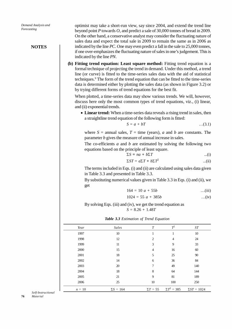
Self-Instructional76 Material
Demand Analysis andForecasting
NOTES
optimist may take a short-run view, say since 2004, and extend the trend linebeyond point P towards O, and predict a sale of 30,000 tonnes of bread in 2009.On the other hand, a conservative analyst may consider the fluctuating nature ofsales data and expect the total sale in 2009 to remain the same as in 2006 asindicated by the line PC. One may even predict a fall in the sale to 25,000 tonnes,if one over-emphasizes the fluctuating nature of sales in one’s judgement. This isindicated by the line PN.
(b) Fitting trend equation: Least square method: Fitting trend equation is aformal technique of projecting the trend in demand. Under this method, a trendline (or curve) is fitted to the time-series sales data with the aid of statisticaltechniques.9 The form of the trend equation that can be fitted to the time-seriesdata is determined either by plotting the sales data (as shown in Figure 3.2) orby trying different forms of trend equations for the best fit.When plotted, a time-series data may show various trends. We will, however,discuss here only the most common types of trend equations, viz., (i) linear,and (ii) exponential trends.
• Linear trend: When a time-series data reveals a rising trend in sales, thena straightline trend equation of the following form is fitted:
S = a + bT …(3.1)
where S = annual sales, T = time (years), a and b are constants. Theparameter b gives the measure of annual increase in sales.The co-efficients a and b are estimated by solving the following twoequations based on the principle of least square.
ΣS = na + bΣT ...(i)ΣST = aΣT + bΣT2 ...(ii)
The terms included in Eqs. (i) and (ii) are calculated using sales data givenin Table 3.3 and presented in Table 3.3.By substituting numerical values given in Table 3.3 in Eqs. (i) and (ii), weget
164 = 10 a + 55b …(iii)1024 = 55 a + 385b …(iv)
By solving Eqs. (iii) and (iv), we get the trend equation asS = 8.26 + 1.48T
Table 3.3 Estimation of Trend Equation
Year Sales T T2 ST
1997 10 1 1 101998 12 2 4 241999 11 3 9 332000 15 4 16 602001 18 5 25 902002 14 6 36 842003 20 7 49 1402004 18 8 64 1442005 21 9 81 1892006 25 10 100 250
n = 10 ΣS = 164 ΣT = 55 ΣT2 = 385 ΣST = 1024
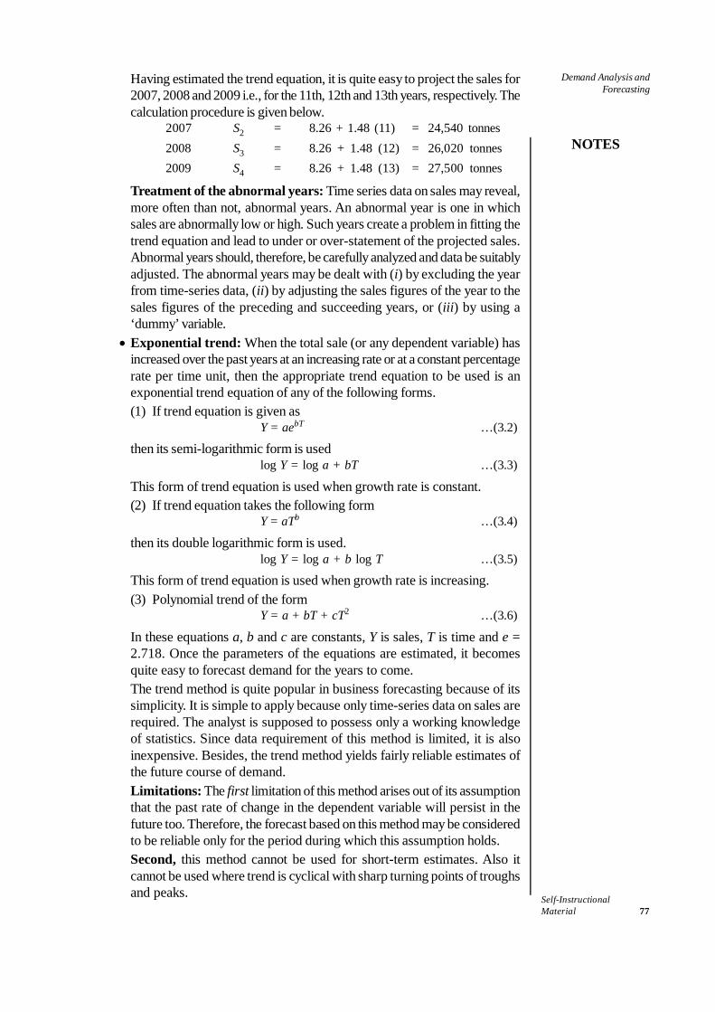
Self-InstructionalMaterial 77
Demand Analysis andForecasting
NOTES
Having estimated the trend equation, it is quite easy to project the sales for2007, 2008 and 2009 i.e., for the 11th, 12th and 13th years, respectively. Thecalculation procedure is given below.
2007 S2 = 8.26 + 1.48 (11) = 24,540 tonnes2008 S3 = 8.26 + 1.48 (12) = 26,020 tonnes2009 S4 = 8.26 + 1.48 (13) = 27,500 tonnes
Treatment of the abnormal years: Time series data on sales may reveal,more often than not, abnormal years. An abnormal year is one in whichsales are abnormally low or high. Such years create a problem in fitting thetrend equation and lead to under or over-statement of the projected sales.Abnormal years should, therefore, be carefully analyzed and data be suitablyadjusted. The abnormal years may be dealt with (i) by excluding the yearfrom time-series data, (ii) by adjusting the sales figures of the year to thesales figures of the preceding and succeeding years, or (iii) by using a‘dummy’ variable.
• Exponential trend: When the total sale (or any dependent variable) hasincreased over the past years at an increasing rate or at a constant percentagerate per time unit, then the appropriate trend equation to be used is anexponential trend equation of any of the following forms.(1) If trend equation is given as
Y = aebT …(3.2)
then its semi-logarithmic form is usedlog Y = log a + bT …(3.3)
This form of trend equation is used when growth rate is constant.(2) If trend equation takes the following form
Y = aTb …(3.4)
then its double logarithmic form is used.log Y = log a + b log T …(3.5)
This form of trend equation is used when growth rate is increasing.(3) Polynomial trend of the form
Y = a + bT + cT2 …(3.6)
In these equations a, b and c are constants, Y is sales, T is time and e =2.718. Once the parameters of the equations are estimated, it becomesquite easy to forecast demand for the years to come.The trend method is quite popular in business forecasting because of itssimplicity. It is simple to apply because only time-series data on sales arerequired. The analyst is supposed to possess only a working knowledgeof statistics. Since data requirement of this method is limited, it is alsoinexpensive. Besides, the trend method yields fairly reliable estimates ofthe future course of demand.Limitations: The first limitation of this method arises out of its assumptionthat the past rate of change in the dependent variable will persist in thefuture too. Therefore, the forecast based on this method may be consideredto be reliable only for the period during which this assumption holds.Second, this method cannot be used for short-term estimates. Also itcannot be used where trend is cyclical with sharp turning points of troughsand peaks.

Self-Instructional78 Material
Demand Analysis andForecasting
NOTES
Third, this method, unlike regression analysis, does not bring out the measureof relationship between dependent and independent variables. Hence, itdoes not yield the necessary information (e.g., price and income elasticities)that can be used for future policy formulations. These limitations need to beborne in mind while making the use of this method.
(c) Box-Jenkins method: Box-Jenkins method10 of forecasting is used onlyfor short-term projections and predictions. Besides, this method is suitablefor forecasting demand with only stationary time-series sales data. Stationarytime-series data is one that does not reveal a long-term trend. In otherwords, Box-Jenkins technique can be used only in those cases in whichtime-series analysis depicts monthly or seasonal variations recurring withsome degree of regularity.When sales data of various commodities are plotted, many commoditieswill show a seasonal or temporal variation in sales. For examples, sale ofwoollen clothes will show a hump during months of winter in all the yearsunder reference. The sale of new year greeting cards will be particularlyhigh in the last week of December every year. Similarly, the sale of desertcoolers is very high during the summers each year. This is called seasonalvariation. Box-Jenkins technique is used for predicting demand wheretime-series sales data reveals this kind of seasonal variation.According to the Box-Jenkins approach, any stationary time-series datacan be analyzed by the following three models:• Autoregression model• Moving average model• Autoregressive-moving average model
The autoregressive-moving average model is the final form of the Box-Jenkins model. The three models are, in fact, the three stages of Box-Jenkins method. The purpose of the three models of Box-Jenkins methodis to explain movements in the stationary series with minimized error term,i.e., the unexplained components of stationary series.The steps and models of the Box-Jenkins approach are described brieflyhere with the purpose of introducing Box-Jenkins method to the readerrather than providing the entire methodology.11
Steps in Box-Jenkins approach: As mentioned above, Box-Jenkinsmethod can be applied only to stationary time-series data. Therefore, thefirst step in Box-Jenkins approach is to eliminate trend from the timeseries data. Trend is eliminated by taking first differences of time-seriesdata, i.e., subtracting observed value of one period from the observedvalue of the preceding year. After trend is elimated, a stationary time-seriesis created.The second step in the Box-Jenkins approach is to make sure that there isseasonality in the stationary time-series. If a certain pattern is found torepeat over time, there is seasonality in the stationary time-series.The final step is to use the models to predict sales in the intended period.We give here a brief description of the Box-Jenkins models that are usedin the same sequence.
• Autoregressive Model: In a general autoregressive model, thebehaviour of a variable in a period is linked to the behaviour of the
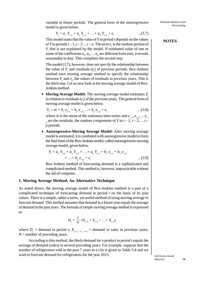
Self-InstructionalMaterial 79
Demand Analysis andForecasting
NOTES
variable in future periods. The general form of the autoregressivemodel is given below.
Yt = a1 Yt–1 + a2 Yt–2 + …+ an Yt–n + et ...(3.7)This model states that the value of Y in period t depends on the valuesof Y in periods t – 1, t – 2 …t – n. The term et is the random portion ofYt that is not explained by the model. If estimated value of one orsome of the coefficients a1, a2, …an are different from zero, it revealsseasonality in data. This completes the second step.The model (3.7), however, does not specify the relationship betweenthe value of Yt and residuals (et) of previous periods. Box-Jenkinsmethod uses moving average method to specify the relationshipbetween Yt and et, the values of residuals in previous years. This isthe third step. Let us now look at the moving average model of Box-Jenkins method.
• Moving Average Model: The moving average model estimates Ytin relation to residuals (et) of the previous years. The general form ofmoving average model is given below. Yt = m + b1 et–1 + b2 et–2 …+ bp et–p + et ...(3.8)where m is the mean of the stationary time-series and et–1, et–2, …et–
p are the residuals, the random components of Y in t – 1, t – 2, …t –p periods.
• Autoregressive-Moving Average Model: After moving averagemodel is estimated, it is combined with autoregressive model to formthe final form of the Box-Jenkins model, called autoregressive-movingaverage model, given below.
Yt = a1 Yt–1 + a2 Yt–2 + …+ an Yt–n + b1 et–1 + b2 et–2
+ …+ bp et–p + et …(3.9)Box-Jenkins method of forecasting demand is a sophisticated andcomplicated method. This method is, however, impracticable withoutthe aid of computer.
1. Moving Average Method: An Alternative Technique
As noted above, the moving average model of Box-Jenkins method is a part of acomplicated technique of forecasting demand in period t on the basis of its pastvalues. There is a simple, rather a naïve, yet useful method of using moving average toforecast demand. This method assumes that demand in a future year equals the averageof demand in the past years. The formula of simple moving average method is expressedas
Dt = 1N
(Xt–1 + Xt–2 + …+ Xt–n)
where Dt = demand in period t; Xt–1, t–2 …t–n = demand or sales in previous years;N = number of preceding years.
According to this method, the likely demand for a product in period t equals theaverage of demand (sales) in several preceding years. For example, suppose that thenumber of refrigerators sold in the past 7 years in a city is given as Table 3.4 and wewant to forecast demand for refrigerators for the year 2015.
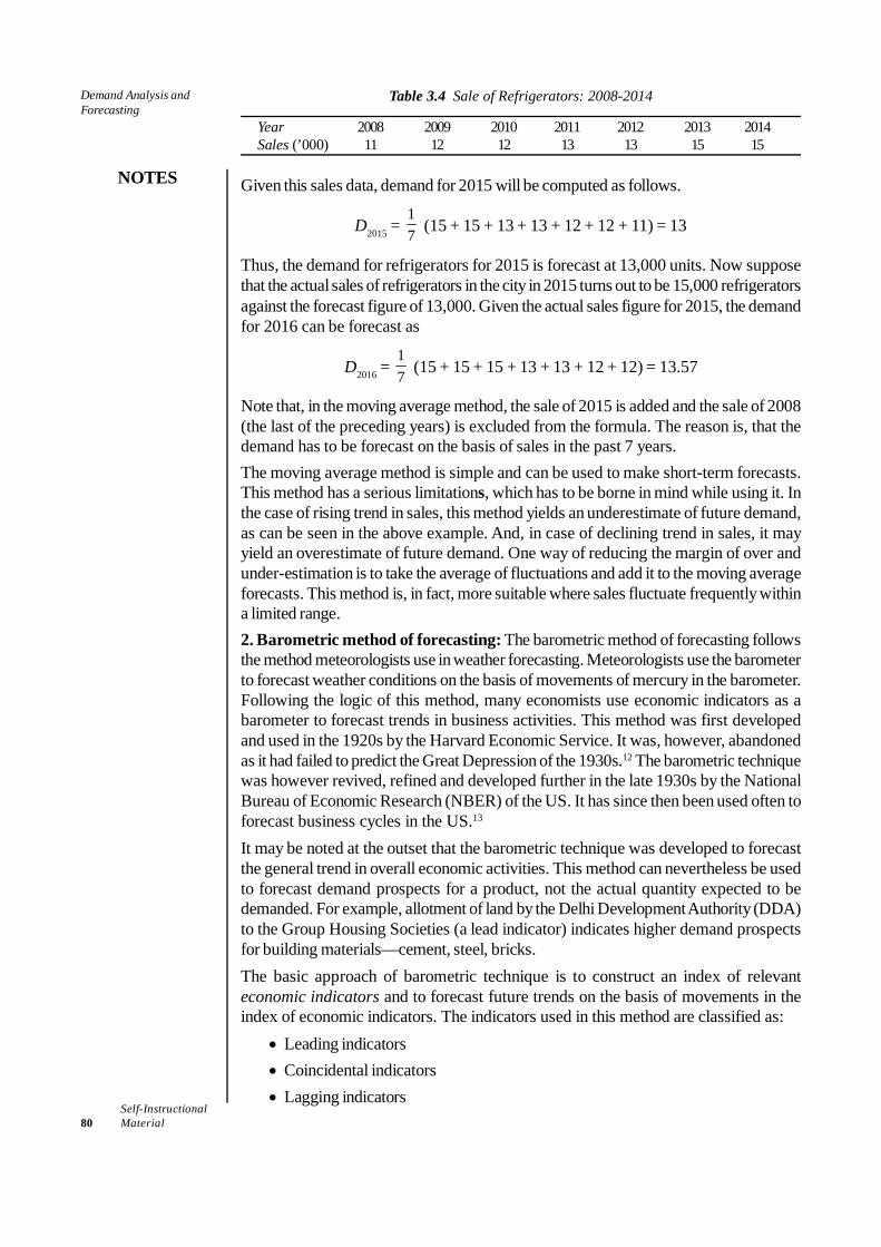
Self-Instructional80 Material
Demand Analysis andForecasting
NOTES
Table 3.4 Sale of Refrigerators: 2008-2014
Year 2008 2009 2010 2011 2012 2013 2014Sales (’000) 11 12 12 13 13 15 15
Given this sales data, demand for 2015 will be computed as follows.
D2015 = 17 (15 + 15 + 13 + 13 + 12 + 12 + 11) = 13
Thus, the demand for refrigerators for 2015 is forecast at 13,000 units. Now supposethat the actual sales of refrigerators in the city in 2015 turns out to be 15,000 refrigeratorsagainst the forecast figure of 13,000. Given the actual sales figure for 2015, the demandfor 2016 can be forecast as
D2016 = 17 (15 + 15 + 15 + 13 + 13 + 12 + 12) = 13.57
Note that, in the moving average method, the sale of 2015 is added and the sale of 2008(the last of the preceding years) is excluded from the formula. The reason is, that thedemand has to be forecast on the basis of sales in the past 7 years.The moving average method is simple and can be used to make short-term forecasts.This method has a serious limitations, which has to be borne in mind while using it. Inthe case of rising trend in sales, this method yields an underestimate of future demand,as can be seen in the above example. And, in case of declining trend in sales, it mayyield an overestimate of future demand. One way of reducing the margin of over andunder-estimation is to take the average of fluctuations and add it to the moving averageforecasts. This method is, in fact, more suitable where sales fluctuate frequently withina limited range.2. Barometric method of forecasting: The barometric method of forecasting followsthe method meteorologists use in weather forecasting. Meteorologists use the barometerto forecast weather conditions on the basis of movements of mercury in the barometer.Following the logic of this method, many economists use economic indicators as abarometer to forecast trends in business activities. This method was first developedand used in the 1920s by the Harvard Economic Service. It was, however, abandonedas it had failed to predict the Great Depression of the 1930s.12 The barometric techniquewas however revived, refined and developed further in the late 1930s by the NationalBureau of Economic Research (NBER) of the US. It has since then been used often toforecast business cycles in the US.13
It may be noted at the outset that the barometric technique was developed to forecastthe general trend in overall economic activities. This method can nevertheless be usedto forecast demand prospects for a product, not the actual quantity expected to bedemanded. For example, allotment of land by the Delhi Development Authority (DDA)to the Group Housing Societies (a lead indicator) indicates higher demand prospectsfor building materials—cement, steel, bricks.The basic approach of barometric technique is to construct an index of relevanteconomic indicators and to forecast future trends on the basis of movements in theindex of economic indicators. The indicators used in this method are classified as:
• Leading indicators• Coincidental indicators• Lagging indicators

Self-InstructionalMaterial 81
Demand Analysis andForecasting
NOTES
A time-series of various indicators is prepared to read the future economic trend. Theleading series consists of indicators which move up or down ahead of some otherseries. Some examples of leading indicators are: (i) index of net business investment;(ii) new orders for durable goods; (iii) change in the value of inventories; (iv) index ofthe prices of the materials; and (v) corporate profits after tax.
The coincidental series, on the other hand, are the ones that move up or downsimultaneously with the level of general economic activities. Some examples of thecoincidental series are: (i) number of employees in the non-agricultural sector; (ii) rateof unemployment; (iii) gross national product at constant prices; and (iv) sales recordedby the manufacturing, trading and the retail sectors.
The lagging series, consist of those indicators that follow a change after sometime-lag. Some of the indices that have been identified as lagging series by the NBERare: (i) labour cost per unit of manufactured output, (ii) outstanding loans, and(iii) lending rate for short-term loans.The various indicators are chosen on the basis of the following criteria:
• Economic significance of the indicator: the greater the significance, the greaterthe score of the indicator
• Statistical adequacy of time-series indicators: a higher score is given to anindicator provided with adequate statistics
• Conformity with overall movement in economic activities• Consistency of series to the turning points in overall economic activity• Immediate availability of the series• Smoothness of the series
The problem of choice may arise because some of the indicators appear in more thanone class of indicators. Furthermore, it is not advisable to rely on just one of theindicators. This leads to the usage of what is referred to as the diffusion index. Adiffusion index is the percentage of rising indicators. A diffusion index copes up withthe problem of differing signals given by the indicators. In calculating a diffusionindex, for a group of indicators, scores allotted are 1 to rising series, ½ to constantseries and zero to falling series. The diffusion index is obtained by the ratio of thenumber of indicators, in a particular class, moving up or down to the total number ofindicators in that group. Thus, if three out of six indicators in the lagging series aremoving up, the index shall be 50 per cent. It may be noted that the most important oneis the diffusion index of the leading series. However, there are problems of identifyingthe leading indicator for the variables under study.
Leading indicators can be used as inputs for forecasting aggregate economicvariables, GNP, aggregate consumers’ expenditure, aggregate capital expenditure, etc.The only advantage of this method is that it overcomes the problem of forecasting thevalue of independent variable under the regression method. The major limitations ofthis method are: (i) it can be used only for short-term forecasting, and (ii) a leadingindicator of the variable to be forecast is not always easily available.3. Econometric methods: The econometric methods combine statistical tools witheconomic theories to estimate economic variables and to forecast the intended economicvariables. The forecasts made through econometric methods are much more reliablethan those made through any other method. The econometric methods are, therefore,most widely used to forecast demand for a product, for a group of products and for
Self-Instructional82 Material
Demand Analysis andForecasting
NOTES
the economy as a whole. We explain here briefly the use of econometric methods forforecasting demand for a product.
An econometric model may be a single-equation regression model or it mayconsist of a system of simultaneous equations. Single-equation regression serves thepurpose of demand forecasting in the case of most commodities. But, whereexplanatory economic variables are so interrelated and interdependent that unless oneis determined, the other cannot be determined, a single-equation regression modeldoes not serve the purpose. In that case, a system of simultaneous equations is usedto estimate and forecast the target variable.The econometric methods are briefly described here under two basic methods.
• Regression method• Simultaneous equations model
These methods are explained here brieflyRegression method: Regression analysis is the most popular method of demandestimation. This method combines economic theory and statistical techniques ofestimation. Economic theory is employed to specify the determinants of demand andto determine the nature of the relationship between the demand for a product and itsdeterminants. Economic theory, thus, helps in determining the general form of demandfunction. Statistical techniques are employed to estimate the values of parameters inthe estimated equation.
In regression technique of demand forecasting, one needs to estimate the demandfunction for a product. While estimating a demand function, demand is a ‘dependentvariable’ and the variables that determine the demand are called ‘independent’ or‘explanatory’ variables. For example, demand for cold drinks in a city may be said todepend largely on ‘per capita income’ of the city and its population. Here demand forcold drinks is a ‘dependent variable’ and ‘per capita income’ and ‘population’ are the‘explanatory’ ‘variables.’
While specifying the demand functions for various commodities, the analystmay come across many commodities whose demand depends, by and large, on asingle independent variable. For example, suppose in a city, demand for such items assalt and sugar is found to depend largely on the population of the city. If this is so,then demand functions for salt and sugar are single-variable demand functions. Onthe other hand, the analyst may find that demand for sweets, fruits and vegetables, etc.depends on a number of variables like commodity’s own price, price of its substitutes,household incomes, population. Such demand functions are called multi-variabledemand functions. For a single-variable demand function, simple regression equationis used and for multiple variable functions, multi-variable equation is used for estimatingdemand function. The single-variable and multi-variable regressions are explained below.(a) Simple or bivariate regression technique: In simple regression technique, asingle independent variable is used to estimate a statistical value of the ‘dependentvariable’, that is, the variable to be forecast. The technique is similar to trend fitting.An important difference between the two is that in trend fitting, the independent variableis ‘time’ (t) whereas in a regression equation, the chosen independent variable is thesingle most important determinant of demand. Besides, the regression method is lessmechanical than the trend fitting method of projection.
Suppose we have to forecast demand for sugar for a country for 2014-15 on thebasis of 7-year data given in Table 3.5. When this data is graphed, it produces a

Self-InstructionalMaterial 83
Demand Analysis andForecasting
NOTES
continuously rising trend in demand for sugar with rising population. This shows a lineartrend. Now, country’s demand for sugar in 2014-15 can be obtained by estimating aregression equation of the form
Y = a + bX …(3.10)
where Y is sugar consumed, X is population, and a and b are the two parameters.For an illustration, consider the hypothetical data on a country’s annual consumption
of sugar given in Table 3.5.
Table 3.5 Annual Consumption of Sugar
Year Population (millions) Sugar Consumed (million tonnes)
2008–07 10 402009–08 12 502011–09 15 602010–11 20 702011–12 25 802012–13 30 902013–14 40 100
Equation (3.10) can be estimated by using the ‘least square’ method. The procedure isthe same as shown in Table 3.3. That is, the parameters a and b can be estimated bysolving the following two linear equations:
ΣYi = na + bΣXi …(i)ΣXiYi = ΣXi a + bX2
i …(ii)
The procedure of calculating the terms in Eqs. (i) and (ii) above is presented inTable 3.6.
Table 3.6 Calculation of Terms of the Linear Equations
(Figures in million)
Year Population Sugar X2 XY(X) consumed (Y)
2008–07 10 40 100 4002009–08 12 50 144 6002011–09 15 60 225 9002010–11 20 70 400 14002011–12 25 80 625 20002012–13 30 90 900 27002013–14 40 100 1600 4000
Σn = 7 ΣXi = 152 ΣYi = 490 ΣXi2 = 3994 ΣXiYi = 12000
By substituting the values from Table 3.6 into Eqs. (i) and (ii), we get490 = 7a + 152b …(iii)12,000 = 152a + 3994b …(iv)
By solving Eqs. (iii) and (iv), we geta = 27.44 and b = 1.96
By substituting values for a and b in Eq. (3.10), we get the estimated regressionequation as
Y = 27.44 + 1.96 X ...(3.11)
Given the regression Eq. (3.11), the demand for sugar for 2014-15 can be easily projectedif population for 2014-15 can be known. Supposing population for 2014-15 is projected tobe 50 million, the demand for sugar of the same year can be estimated as follows.
Self-Instructional84 Material
Demand Analysis andForecasting
NOTES
Y = 27.44 + 1.96(50) = 126 million tonnes
The simple regression technique is based on the assumptions (i) that independent variablewill continue to grow at its past growth rate, and (ii) that the relationship between thedependent and independent variables will continue to remain the same in the future as inthe past. (For further details and for the test of the reliability of estimates, consult astandard book on statistics).(b) Multi-variate regression: The multi-variate regression equation is used wheredemand for a commodity is considered to be a function of explanatory variablesgreater than one.
The procedure of multiple regression analysis is briefly described here. Thefirst step in multiple regression analysis is to specify the variables that are supposed toexplain the variations in demand for the product under reference. The explanatoryvariables are generally chosen from the determinants of demand, viz., price of theproduct, price of its substitutes, consumers’ income and their tastes and preferences.For estimating the demand for durable consumer goods, (e.g., TV sets, refrigerators,houses), the other explanatory variables that are considered are availability of creditand rate of interest. For estimating demand for capital goods (e.g., machinery andequipment), the relevant variables are additional corporate investment, rate ofdepreciation, cost of capital goods, cost of other inputs (e.g., labour and raw materials),market rate of interest.
Once the explanatory or independent variables are specified, the second step isto collect time-series data on the independent variables. After necessary data is collected,the third and a very important step is to specify the form of equation which canappropriately describe the nature and extent of relationship between the dependentand independent variables. The final step is to estimate the parameters in the chosenequation with the help of statistical techniques. The multi-variate equation cannot beeasily estimated manually. Therefore, the equation has to be estimated with the help ofa computer.Specifying the form of equation: The reliability of the demand forecast depends to alarge extent on the form of equation and the degree of consistency of the explanatoryvariables in the estimated demand function. The greater the degree of consistency, thehigher the reliability of the estimated demand and vice versa. Adequate precautionshould, therefore, be taken in specifying the equation to be estimated. Some commonforms of multi-variate demand functions are given below.Linear function: Where the relationship between demand and its determinants isgiven by a linear equation, the most common form of equation used for estimatingdemand is given below.
Qx = a – bPx + cY + dPy + jA …(3.12)
where Qx = quantity demanded of commodity X; Px = price of commodity X; Y =consumers’ income, Py = price of the substitute; A = advertisement expenditure; a is aconstant (the intercept), and b, c, d and j are the parameters expressing the relationshipbetween demand and Px, Y, Py and A, respectively.
In a linear demand function, quantity demanded is assumed to change at aconstant rate with a change in independent variables Px, Y, Py and A. The parameters(regression co-efficients) are estimated by using the least square method. After parametersare estimated, the demand can be easily forecast if data on independent variables for the
Self-InstructionalMaterial 85
Demand Analysis andForecasting
NOTES
reference period is available. Suppose, the estimated equation for sugar takes the followingform:
Qs = 50 – 0.75Ps + 0.1Y + 1.25 Py + 0.05A …(3.13)
The numerical values in this equation express the quantitative relationship14 betweendemand for sugar and the variables with which it is associated. More precisely, regressionco-efficients give the change in demand for sugar as a result of unit change in theexplanatory variables. For instance, it reveals that a change of one rupee in the sugarprice results in a 0.75 tonne change in sugar demand and a change of one rupee inincome leads to a 0.1 tonne change in sugar demand, and so on.Power function: It may be noted that in linear Eq. (3.12), the marginal effect ofindependent variables on demand is assumed to be constant and independent of changein other variables. For example, it assumes that the marginal effect of change in price isindependent of change in income or other independent variables, and so on. However,one can find cases in which it is theoretically and also empirically found that themarginal effect of the independent variables on demand is neither constant norindependent of the value of all other variables included in the demand function. Forexample, the effect of rise in sugar price may be neutralized by a rise in consumersincome. In such cases, a multiplicative form of equation which is considered to be‘the most logical form of demand function’ is used for estimating demand for a product.The multiplicative form of demand function or power function is given as
Qx = a Px–b Yc Py
d Aj …(3.14)
The algebraic form of multiplicative demand function can be transformed into a log-linear form for convenience in estimation, as given below.
log Qx = log a – b log Px + c log Y + d log Py + j log A …(3.15)
The log-linear demand function can be estimated by the least square regression technique.The estimated function yields the intercept a and the values of the regression co-efficients. After regression co-efficients are estimated and data on the independentvariables for the years to come are obtained, forecasting demand becomes an easytask.Reliability of estimates: As mentioned earlier, statistical methods are scientific, devoidof subjectivity, and they yield fairly reliable estimates. But the reliability of forecastdepends also on a number of other factors.
A very important factor in this regard is the choice of the right kind of variablesand data. Only those independent variables which have a causal relationship betweenthe dependent and independent variables should be included in the demand function.The relationship between the dependent and independent variables should be clearlydefined.
Besides, the reliability of estimates also depends on the form of demand functionused. The forecaster should, therefore, bear in mind that there is no hard and fast ruleand an a priori basis of determining the most appropriate form of demand function.The demand function to be estimated is generally determined by testing different formsof functions. Whether a particular form of function is a good fit is judged by thecoefficient of determination, i.e., the value of R2. The value of R2 gives the proportionof the total variation in the dependent variable explained by the variation in theindependent variables. The higher the value of R2, the greater the explanatory power ofthe independent variables.

Self-Instructional86 Material
Demand Analysis andForecasting
NOTES
Another test is the expected sign of co-efficients of independent variables. Whatis more important, therefore, is to carefully ascertain the theoretical relationship betweenthe dependent and the independent variables.Simultaneous equations model: We may recall that regression technique of demandforecasting consists of a single equation. In contrast, the simultaneous equations modelof forecasting involves estimating several simultaneous equations. These equationsare, generally, behavioural equations, mathematical identities and market-clearingequations.
Furthermore, regression technique assumes one-way causation, i.e., only theindependent variables cause variations in the dependent variable, not vice versa. Insimple words, regression technique assumes that a dependent variable affects in noway the independent variables. For example, in demand function D = a – bP used inthe regression method, it is assumed that price affects demand, but demand does notaffect price. This is an unrealistic assumption. On the contrary, forecasting througheconometric models of simultaneous equations enables the forecaster to take intoaccount the simultaneous interaction between dependent and independent variables.
The simultaneous equations method is a complete and systematic approach toforecasting. This technique uses sophisticated mathematical and statistical tools thatare beyond the scope of this book15. We will, therefore, restrict ourselves here only tothe basic features of this method of forecasting.
The first step in this technique is to develop a complete model and specify thebehavioural assumptions regarding the variables included in the model. The variablesthat are included in the model are called (i) endogenous variables, and(ii) exogenous variables.Endogenous variables: The variables that are determined within the model are calledendogenous variables. These are included in the model as dependent variables, i.e.,the variables that are to be explained by the model. These are also called ‘controlled’variables. It is important to note that the number of equations included in the modelmust equal the number of endogenous variables.Exogenous variables: Exogenous variables are those that are determined outside themodel. These are inputs of the model. Whether a variable is treated as endogenous orexogenous depends on the purpose of the model. The examples of exogenous variablesare ‘money supply, ‘tax rates’, ‘government spending’, ‘time’, and ‘weather’, etc.The exogenous variables are also known as ‘uncontrolled’ variables.
The second step in this method is to collect the necessary data on bothendogenous and exogenous variables. More often than not, data is not available in therequired form. Sometimes data is not available at all. In such cases, data has to beadjusted or corrected to suit the model and, in some cases, data has to be evengenerated from the available primary or secondary sources.
After the model is developed and necessary data are collected, the third step isto estimate the model through some appropriate method. Generally, a two-stage leastsquare method is used to predict the values of exogenous variables.
Finally, the model is solved for each endogenous variable in terms of exogenousvariables. Then by plugging the values of exogenous variables into the equations, theobjective value is calculated and prediction is made.
Self-InstructionalMaterial 87
Demand Analysis andForecasting
NOTES
Example
For an example, consider a simple macroeconomic model, given below:Yt = Ct + It + Gt + NXt …(3.16)
whereYt = Gross national product,Ct = Total consumption expenditure,It = Gross private investment,Gt = Government expenditure,NXt = Net exports (X – M) where M = imports and subscript t represents a
given time unit.Equation (3.16) is an identity, that may be explained with a system of simultaneousequations. Suppose in Eq. (3.16)
Ct = a + bYt ...(3.17)It = 20 ...(3.18)Gt = 10 ...(3.19)NX = 5 ...(3.20)
In the above system of equations, Yt and Ct are endogenous variables and It, Gt andNXt are exogenous variables. Eq. (3.17) is a regression equation that has to be estimated.Equations (3.18), (3.19) and (3.20) show the values of exogenous variables determinedoutside the model.
Suppose we want to predict the value of Yt and Ct simultaneously. Suppose alsothat when we estimate Eq. (3.17), we get
Ct = 100 + 0.75 Yt ...(3.21)
Now, using this equation system, we may determine the value of Yt asYt = Ct + 20 + 10 + 5 = Ct + 35
Since Ct = 100 + 0.75 Yt, by substitution, we getYt = 100 + 0.75 Yt + 35
then Yt – 0.75 Yt = 100 + 350.25 Yt = 135
and Yt = 135/0.25 = 540
We may now easily calculate the value of Ct (using Yt = 540). SinceCt = 100 + 0.75 Yt = 100 + 0.75 (540) = 505
Thus, the predicted values areYt = 540 and Ct = 505
Thus, Yt = 505 + 20 + 10 + 5 = 540
It is important to note here that the example of the econometric model given above isan extremely simplified model. The econometric models used in actual practice aregenerally very complex. They include scores of simultaneous equations.
However, this method is theoretically superior to the regression method. Themain advantage of this method is that it is capable of capturing the effect ofinterdependence of the variables. But, its limitations are similar to those of the regressionmethod. The use of this method is sometimes hampered by non-availability of adequatedata.
Check Your Progress
4. Define demandforecasting.
5. List the techniquesused under opinionpoll method.
6. What are the threekinds of statisticalmethod used fordemand projection?
7. List the threemodels which helpin the analysis ofstationary time-series data underthe Box-Jenkinsmethod.
8. Define endogenousvariables.
9. What are exogenousvariables?
Self-Instructional88 Material
Demand Analysis andForecasting
NOTES
There are several methods and techniques available for forecasting demand for aproduct. All the methods have their own limitations and advantages, merits and demerits,in varying degrees. The applicability and usefulness of a method depends on the purposeof forecasting and availability of reliable and relevant data. The analyst should, therefore,choose a method or a technique of demand forecasting that is relevant to the purpose,convenient to handle, applicable to the available data and also inexpensive.
It may be added that mere possession of the right tools does not necessarilyensure an accurate forecast. Equally important is the analyst’s own judgement. In fact,the role of analyst’s judgement cannot be over-emphasized. It is required at all stagesof demand forecasting. Any estimate relating to a future period in itself is a judgementand involves a series of judgements. Analyst’s judgement is required in the first placeto ensure that the method used in making the estimate is appropriate to the task. Also,when a statistical series is generated, its interpretation requires judgement.
Besides, several components and elements used in forecasting are often in conflictand are so balanced that they leave little room for choice. Nevertheless, one or theother has to be judged as being appropriate for use under the given circumstances.
Furthermore, events relating to economic activity take place sometimes suddenlyand sometimes in an uneven manner. Without adequate information about the currentsituation, there are bound to be errors of judgement in statistical projections. Mostpeople, if they lack the correct perspective, cannot fathom the significance of evencurrent information unless it is properly related to all concerned activities. Therefore,interpreting the current information or data and making proper use of the same forfuture projection also calls for judgement.
Finally, is should be appreciated that forecasting is merely an attempt to utilizethe generally accepted methods or techniques for knowing the future demand for aproduct. By the very nature of the problem, there can be no guarantee of accuracy inany specified methodology or system of indicators. Hence, it would be unreasonableto be dogmatic about the results obtained or to say that any one particular method issuperior to others. As time proceeds, opportunities are provided for testing the validityof any forecast. A person who has done a forecast should be prepared to recede froma position previously taken whenever it is known that economic and other conditionsthat formed the basis for the previous forecast have changed. The only sound procedureis to correct the previous forecast in as objective a manner as possible. There is needfor continual revision so that forecast gets closer to reality.
3.4 SOME CASE STUDIES OF DEMANDFORECASTING
In this section, we briefly describe some studies in demand forecasting. Not many casestudies with Indian data are available on the various methods of demand forecasting.The case studies that are available mostly use the regression method. The casesdescribed below include some on consumer goods and some on intermediate goods.
Consumer Goods
Eggs: Eggs are one of the popular items of food for non-vegetarians and semi-vegetarians. Sidhu16 estimated demand function for eggs for Ludhiana district of Punjabfor various occupational groups in rural and urban areas. We will consider here only
Check Your Progress
10. Techniques ofdemand forecastinginclude:
(a) Planning andschedulingproduction
(b) Makingprovision forfinances
(c) Formulatingpricing strategy
(d) Survey andStatisticalmethods
11. Regression methodis the most popularmethod of
(a) Forecastingweather
(b) Explainingmovements in thestationary serieswith minimizederror term
(c) Demandelimination
(d) Consolidating thedivergent expertopinions andarrive at acompromiseestimate of futuredemand
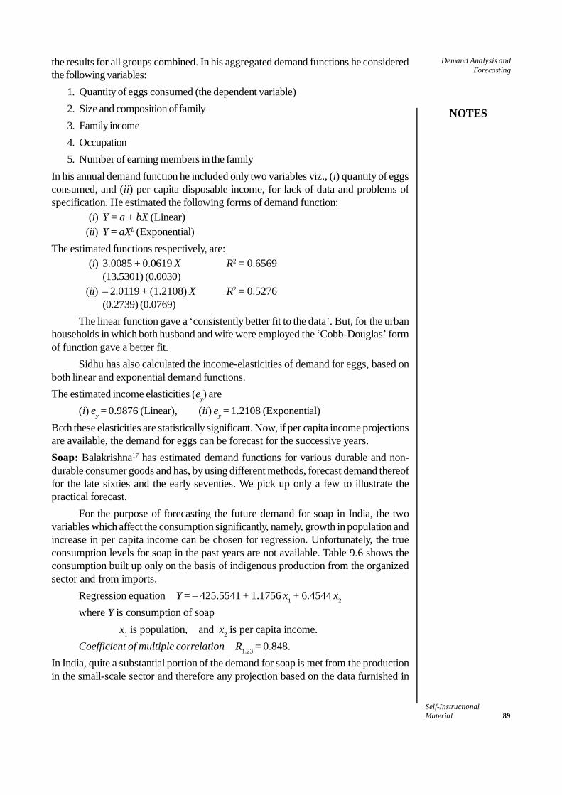
Self-InstructionalMaterial 89
Demand Analysis andForecasting
NOTES
the results for all groups combined. In his aggregated demand functions he consideredthe following variables:
1. Quantity of eggs consumed (the dependent variable)2. Size and composition of family3. Family income4. Occupation5. Number of earning members in the family
In his annual demand function he included only two variables viz., (i) quantity of eggsconsumed, and (ii) per capita disposable income, for lack of data and problems ofspecification. He estimated the following forms of demand function:
(i) Y = a + bX (Linear)(ii) Y = aXb (Exponential)
The estimated functions respectively, are:(i) 3.0085 + 0.0619 X R2 = 0.6569
(13.5301) (0.0030)(ii) – 2.0119 + (1.2108) X R2 = 0.5276
(0.2739) (0.0769)The linear function gave a ‘consistently better fit to the data’. But, for the urban
households in which both husband and wife were employed the ‘Cobb-Douglas’ formof function gave a better fit.
Sidhu has also calculated the income-elasticities of demand for eggs, based onboth linear and exponential demand functions.The estimated income elasticities (ey) are
(i) ey = 0.9876 (Linear), (ii) ey = 1.2108 (Exponential)Both these elasticities are statistically significant. Now, if per capita income projectionsare available, the demand for eggs can be forecast for the successive years.Soap: Balakrishna17 has estimated demand functions for various durable and non-durable consumer goods and has, by using different methods, forecast demand thereoffor the late sixties and the early seventies. We pick up only a few to illustrate thepractical forecast.
For the purpose of forecasting the future demand for soap in India, the twovariables which affect the consumption significantly, namely, growth in population andincrease in per capita income can be chosen for regression. Unfortunately, the trueconsumption levels for soap in the past years are not available. Table 9.6 shows theconsumption built up only on the basis of indigenous production from the organizedsector and from imports.
Regression equation Y = – 425.5541 + 1.1756 x1 + 6.4544 x2
where Y is consumption of soapx1 is population, and x2 is per capita income.
Coefficient of multiple correlation R1.23 = 0.848.In India, quite a substantial portion of the demand for soap is met from the productionin the small-scale sector and therefore any projection based on the data furnished in
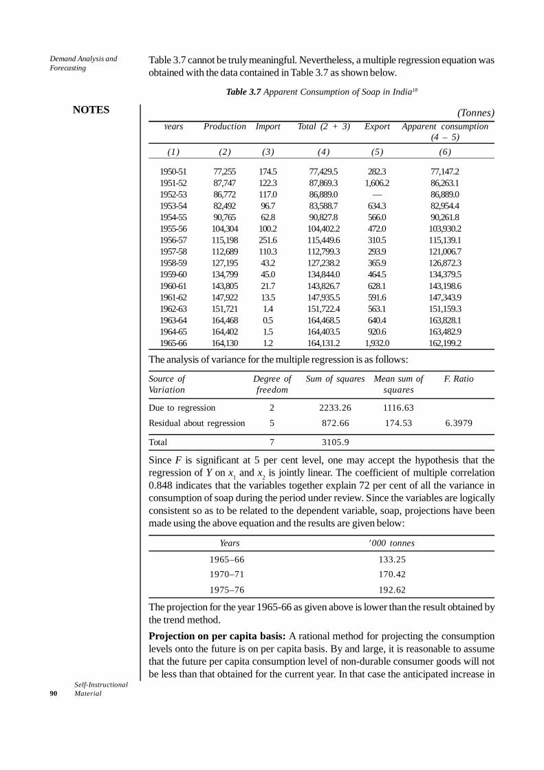
Self-Instructional90 Material
Demand Analysis andForecasting
NOTES
Table 3.7 cannot be truly meaningful. Nevertheless, a multiple regression equation wasobtained with the data contained in Table 3.7 as shown below.
Table 3.7 Apparent Consumption of Soap in India18
(Tonnes)Years Production Import Total (2 + 3) Export Apparent consumption
(4 – 5)(1) (2) (3) (4) (5) (6)
1950-51 77,255 174.5 77,429.5 282.3 77,147.21951-52 87,747 122.3 87,869.3 1,606.2 86,263.11952-53 86,772 117.0 86,889.0 — 86,889.01953-54 82,492 96.7 83,588.7 634.3 82,954.41954-55 90,765 62.8 90,827.8 566.0 90,261.81955-56 104,304 100.2 104,402.2 472.0 103,930.21956-57 115,198 251.6 115,449.6 310.5 115,139.11957-58 112,689 110.3 112,799.3 293.9 121,006.71958-59 127,195 43.2 127,238.2 365.9 126,872.31959-60 134,799 45.0 134,844.0 464.5 134,379.51960-61 143,805 21.7 143,826.7 628.1 143,198.61961-62 147,922 13.5 147,935.5 591.6 147,343.91962-63 151,721 1.4 151,722.4 563.1 151,159.31963-64 164,468 0.5 164,468.5 640.4 163,828.11964-65 164,402 1.5 164,403.5 920.6 163,482.91965-66 164,130 1.2 164,131.2 1,932.0 162,199.2
The analysis of variance for the multiple regression is as follows:
Source of Degree of Sum of squares Mean sum of F. RatioVariation freedom squares
Due to regression 2 2233.26 1116.63
Residual about regression 5 872.66 174.53 6.3979
Total 7 3105.9
Since F is significant at 5 per cent level, one may accept the hypothesis that theregression of Y on x1 and x2 is jointly linear. The coefficient of multiple correlation0.848 indicates that the variables together explain 72 per cent of all the variance inconsumption of soap during the period under review. Since the variables are logicallyconsistent so as to be related to the dependent variable, soap, projections have beenmade using the above equation and the results are given below:
Years ′000 tonnes
1965–66 133.251970–71 170.42
1975–76 192.62
The projection for the year 1965-66 as given above is lower than the result obtained bythe trend method.Projection on per capita basis: A rational method for projecting the consumptionlevels onto the future is on per capita basis. By and large, it is reasonable to assumethat the future per capita consumption level of non-durable consumer goods will notbe less than that obtained for the current year. In that case the anticipated increase in
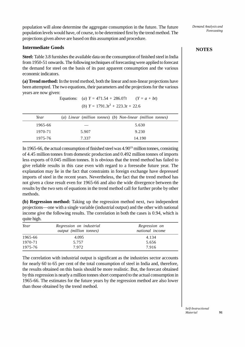
Self-InstructionalMaterial 91
Demand Analysis andForecasting
NOTES
population will alone determine the aggregate consumption in the future. The futurepopulation levels would have, of course, to be determined first by the trend method. Theprojections given above are based on this assumption and procedure.
Intermediate Goods
Steel: Table 3.8 furnishes the available data on the consumption of finished steel in Indiafrom 1950-51 onwards. The following techniques of forecasting were applied to forecastthe demand for steel on the basis of its past apparent consumption and the variouseconomic indicators.(a) Trend method: In the trend method, both the linear and non-linear projections havebeen attempted. The two equations, their parameters and the projections for the variousyears are now given:
Equations: (a) Y = 471.54 + 286.07t (Y = a + bt)
(b) Y = 1791.3t3 + 223.3t + 22.6
Year (a) Linear (million tonnes) (b) Non-linear (million tonnes)
1965-66 — 5.6301970-71 5.907 9.2301975-76 7.337 14.190
In 1965-66, the actual consumption of finished steel was 4.9019 million tonnes, consistingof 4.45 million tonnes from domestic production and 0.492 million tonnes of importsless exports of 0.045 million tonnes. It is obvious that the trend method has failed togive reliable results in this case even with regard to a foreseabe future year. Theexplanation may lie in the fact that constraints in foreign exchange have depressedimports of steel in the recent years. Nevertheless, the fact that the trend method hasnot given a close result even for 1965-66 and also the wide divergence between theresults by the two sets of equations in the trend method call for further probe by othermethods.(b) Regression method: Taking up the regression method next, two independentprojections—one with a single variable (industrial output) and the other with nationalincome give the following results. The correlation in both the cases is 0.94, which isquite high.Year Regression on industrial Regression on
output (million tonnes) national income1965-66 4.095 4.1341970-71 5.757 5.6561975-76 7.972 7.916
The correlation with industrial output is significant as the industries sector accountsfor nearly 60 to 65 per cent of the total consumption of steel in India and, therefore,the results obtained on this basis should be more realistic. But, the forecast obtainedby this regression is nearly a million tonnes short compared to the actual consumption in1965-66. The estimates for the future years by the regression method are also lowerthan those obtained by the trend method.
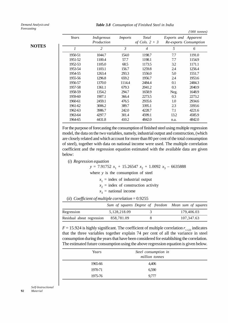
Self-Instructional92 Material
Demand Analysis andForecasting
NOTES
Table 3.8 Consumption of Finished Steel in India
(′000 tonnes)
Years Indigenous Imports Total Exports and ApparentProduction of Cols. 2 + 3 Re-exports Consumption
1 2 3 4 5 6
1950-51 1044.7 154.0 1198.7 7.7 1191.01951-52 1100.4 57.7 1198.1 7.7 1154.91952-53 1105.0 68.5 1173.5 3.2 1171.11953-54 1103.1 156.7 1259.8 2.4 1256.41954-55 1263.4 293.3 1556.0 5.0 1551.71955-56 1296.8 659.2 1956.7 2.4 1953.61956-57 1370.0 1114.4 2484.4 0.1 2484.31957-58 1361.1 679.3 2041.2 0.3 2040.91958-59 1354.2 294.7 1658.9 Neg. 1648.91959-60 1907.1 366.4 2273.5 0.3 2273.21960-61 2459.1 476.5 2935.6 1.0 2934.61961-62 3006.2 389.7 3395.1 2.3 3393.61962-63 3986.7 242.0 4228.7 7.1 4221.61963-64 4297.7 301.4 4599.1 13.2 4585.91964-65 4431.8 410.2 4842.0 n.a. 4842.0
For the purpose of forecasting the consumption of finished steel using multiple regressionmodel, the data on the two variables, namely, industrial output and construction, (whichare closely related and which account for more than 80 per cent of the total consumptionof steel), together with data on national income were used. The multiple correlationcoefficient and the regression equation estimated with the available data are givenbelow:
(i) Regression equationy = 7.91752 x1 + 15.26547 x2 + 1.0092 x3 – 6635888where y is the consumption of steel
x1 = index of industrial outputx2 = index of construction activityx3 = national income
(ii) Coefficient of multiple correlation = 0.9255Sum of squares Degree of freedom Mean sum of squares
Regression 5,128,218.09 3 179,406.03Residual about regression 858,781.09 8 107,347.63
F = 15.924 is highly significant. The coefficient of multiple correlation r1.123 indicatesthat the three variables together explain 74 per cent of all the variance in steelconsumption during the years that have been considered for establishing the correlation.The estimated future consumption using the above regression equation is given below.
Years Steel consumption inmillion tonnes
1965-66 4,4061970-71 6,5901975-76 9,777
Self-InstructionalMaterial 93
Demand Analysis andForecasting
NOTES
It is interesting to observe that the estimate of 1965-66 by multiple regression is closer tothe actual consumption in that year than those obtained either by the trend or by regressionmethod on a single variable, like industrial output or national income.(c) End-use method: Taking up next the results of an end-use study that was carriedout in 1963 for steel consumption,20 the aggregate figures were as follows, for 1965-66and 1970-71. The demand for 1975-76 was not estimated in that study.
Kind of steel 1965-66 1970-71
Finished steel 6.902 135.94
Crude steel 9.735 18.287
There is a difference of two million tonnes between the end-use estimate for 1965-66and the actual consumption of finished steel in that year. A probe into the actual outputin 1965-66, of the industries and other sectors that consume steel, would reveal thefactors accounting for the shortfall. It was found that the shortfall was mostly in theindustrial sector.
3.5 SUMMARY
• The law of demand states the nature of relationship between the quantity demandedof a product and the price of the product.
• Although quantity demanded of a commodity depends also on many other factors,e.g., consumer’s income, price of the substitutes and complementary goods,consumer’s taste and preferences, advertisement, etc., the current price is themost important and the only determinant of demand in the short run.
• A demand schedule is a tabular presentation of different prices of a commodityand its corresponding quantity demanded per unit of time.
• A demand curve is a graphical presentation of the demand schedule. A demandcurve is obtained by plotting a demand schedule.
• Demand forecasting is predicting the future demand for firm’s product.• Survey method includes:
(a) Survey of potential consumers’ plan(b) Opinion poll of experts
• Sample survey method is used when population of the target market is very large.Under sample survey method, only a sample of potential consumers or users isselected for interview.
• The end-use method of demand forecasting has a considerable theoretical andpractical value, especially in forecasting demand for inputs.
• The opinion poll methods aim at collecting opinions of those who are supposed topossess knowledge of the market, e.g., sales representatives, sales executives,professional marketing experts and consultants. The opinion poll methods include:
(a) Expert-opinion method(b) Delphi method(c) Market studies and experiments
• Delphi method of demand forecasting is an extension of the simple expert opinionpoll method. This method is used to consolidate the divergent expert opinions andto arrive at a compromise estimate of future demand.
Self-Instructional94 Material
Demand Analysis andForecasting
NOTES
• Three kinds of statistical methods are used for demand projection.(a) Trend Projection methods,(b) Barometric methods(c) Econometric method
• Trend projection method is a ‘classical method’ of business forecasting. Thismethod is essentially concerned with the study of movement of variables throughtime.
• The barometric method of forecasting follows the method meteorologists usein weather forecasting.
• The econometric methods combine statistical tools with economic theories toestimate economic variables and to forecast the intended economic variables.
• The econometric methods are briefly described here under two basic methods:(a) Regression method(b) Simultaneous equations model
• There are several methods and techniques available for forecasting demand for aproduct. All the methods have their own limitations and advantages, merits anddemerits, in varying degrees. The applicability and usefulness of a method dependson the purpose of forecasting and availability of reliable and relevant data.
3.6 KEY TERMS
• Demand schedule: A demand schedule is a tabular presentation of different pricesof a commodity and its corresponding quantity demanded per unit of time.
• Demand curve: A demand curve is a graphical presentation of the demandschedule. A demand curve is obtained by plotting a demand schedule.
• Demand forecasting: Demand forecasting is predicting the future demand forfirm’s product.
• Endogenous variables: The variables that are determined within the model arecalled endogenous variables.
• Exogenous variables: Exogenous variables are those that are determinedoutside the model. These are inputs of the model.
3.7 ANSWERS TO ‘CHECK YOUR PROGRESS’
1. A demand schedule is a tabular presentation of different prices of a commodityand its corresponding quantity demanded per unit of time.
2. A demand curve is a graphical presentation of the demand schedule. A demandcurve is obtained by plotting a demand schedule.
3. (a) When prices go up, demand goes down4. Demand forecasting is predicting the future demand for firm’s product.5. The opinion poll methods include:
• Expert-opinion method• Delphi method• Market studies and experiments

Self-InstructionalMaterial 95
Demand Analysis andForecasting
NOTES
6. Three kinds of statistical methods are used for demand projection.• Trend projection methods• Barometric methods• Econometric method
7. According to the Box-Jenkins approach, any stationary time-series data can beanalyzed by the following three models:• Autoregression model• Moving average model• Autoregressive-moving average model
8. The variables that are determined within the model are called endogenous variables.9. Exogenous variables are those that are determined outside the model. These are
inputs of the model.10. (d) Survey and Statistical methods11. (c) Demand elimination
3.8 QUESTIONS AND EXERCISES
Short-Answer Questions
1. State the law of demand.2. What are the advantages of end-use method?3. What are the limitations of expert opinion method?4. State the reasons for statistical method being considered a superior technique
of demand estimation.5. What are leading, coincidental and lagging indicators?6. Write short notes on:
(a) Regression method(b) Simultaneous equations model
Long-Answer Questions
1. What are the steps that are undertaken to make demand forecasting systematic?2. Discuss the consumer survey methods.3. Describe the various techniques used under opinion poll methods.4. Discuss the three kinds of statistical methods.
3.9 FURTHER READING/ENDNOTES
Varshney and Maheshwari. 2011. Managerial Economics. New Delhi: Sultan Chandand Sons.
Mankar, V. G. 1982. Business Economics. New Delhi: Himalya Publishing House.Dufty, N.F. 1966. Managerial Economics. New York: Asia Publishing House.
Self-Instructional96 Material
Demand Analysis andForecasting
NOTES
Endnotes
1. Eugene, F. Brigham, and James L. Pappas, Managerial Economics, The DrydenPress, Hinsdale. Illinois, 1976. p. 129.
2. The market segment may be defined in terms of geographical region, income-groupsof the consumers or a particular section of the society (e.g., libraries and studentssegment of market for textbooks).
3. For example, Brigham, Eugene F. and James L. Pappas, op. cit., pp. 548–49.4. The origin of ‘Delphi method’ is traced to Greek mythology. In ancient Greece,
Delphi was an oracle of Apollo and served as a medium for consulting deities. Inmodern times, Delphi method was developed by Olaf Helmer at the Rand Corporationof the US, as a method of obtaining a consensus of panelists without direct interactionbetween them. (J.R. Davis and S. Chang, Managerial Economics (Prentice-Hall,N.J., 1986, p. 191).
5. Brigham, Eugene F. and James, L. Pappas, op. cit., p. 135.6. Webb, Samuel C., Managerial Economics, (Houghton Miffln Company, Boston,
1976), p. 156.7. Dean, J., Managerial Economics, (Englewood Cliffs, N.J., Indian Edn., 1960), p.
181.8. Balakrishna, S., Techniques of Demand Forecasting for Industrial Products, p. 4.9. The statistical technique used to find the trend line, i.e., the ‘least square method’.
10. This method was suggested by G.E.P. Box and G.M. Jenkins in their book, TimeSeries Analysis: Forecasting and Control (Holdan-Day, San Francisco, 1970).
11. Computer programs on Box-Jenkins method are available for use.12. Lange, O., Introduction to Econometrics, 2nd Edn. (Oxford Pergamon Press, 1962),
pp. 85–95.13. A summary of use and findings of this method can be had from R. Davis and
Semoon Chang, Principles of Managerial Economics (Prentice-Hall, NJ, 1986).14. Estimated values of parameters, – 0.75, 0.1, 1.25 and 0.05 are the regression co-
efficients of demand with respect to Px, Y, Py and A, respectively.15. For detailed discussion on the use of econometric methods in business decision, see
J.W. Elliott, Econometric Analysis for Management Decisions (Homewood, Irwin,1973).
16. Sidhu, D.S., Demand and Supply of Eggs: An Economic Analysis (S. Chand & Co.,New Delhi, 1974). The study was made for 1968-69.
17. Balakrishna, S. op. cit.18. Reproduced from Balakrishna, op. cit.19. This does not take into account the steel content of imported machinery and other
finished goods made from steel.20. ‘Reappraisal of Steel Demand’, 1963, National Council for Applied Economics
Research, New Delhi.
Self-InstructionalMaterial 97
Production Function
NOTES
UNIT 4 PRODUCTION FUNCTION
Structure4.0 Introduction4.1 Unit Objectives4.2 Production Function: Concept4.3 Break-even Analysis
4.3.1 Contribution Analysis4.3.2 Profit—Volume Ratio
4.3.3 Margin of Safety4.4 Law of Variable Proportion
4.4.1 Determining Optimum Employment of Labour4.4.2 Isoquant Curves and their Properties4.4.3 Isoquant Map and Economic Region of Production4.4.4 Elasticity of Factor Substitution4.4.5 Laws of Returns to Scale
4.5 Summary4.6 Key Terms4.7 Answers to ‘Check Your Progress’4.8 Questions and Exercises4.9 Further Reading/Endnotes
4.0 INTRODUCTION
Whatever the objective of business firms, achieving optimum efficiency in productionor minimizing cost for a given production is one of the prime concerns of businessmanagers. In fact, the very survival of a firm in a competitive market depends on theirability to produce at a competitive cost. Therefore, managers of business firmsendeavour to minimize the production cost of a given output or, in other words,maximize the output from a given quantity of inputs. In their effort to minimize thecost of production, the fundamental questions that managers are faced with are:
• How can production be optimized or cost minimized?• How does output respond to change in quantity of inputs?• How does technology matter in reducing the cost of production?• How can the least-cost combination of inputs be achieved?• Given the technology, what happens to the rate of return when more plants are
added to the firm?The theory of production provides a theoretical answer to these questions throughabstract models built under hypothetical conditions. The production theory may, therefore,not provide solutions to the real life problems. But it does provide tools and techniques toanalyze the real-life production conditions and to find solutions to the practical businessproblems.
This unit is devoted to the discussion on the theory of production and productionfunction. Production theory deals with quantitative relationships—technical andtechnological relations—between inputs (especially labour and capital) and output.
Self-Instructional98 Material
Production Function
NOTES
4.1 UNIT OBJECTIVES
After going through this unit, you will be able to:• Understand the concept of production function• Explain break-even analysis• Discuss law of variable proportion
4.2 PRODUCTION FUNCTION: CONCEPT
Production function is a mathematical presentation of input-output relationship. Morespecifically, a production function states the technological relationship between inputsand output in the form of an equation, a table or a graph. In its general form, itspecifies the inputs on which depends the production of a commodity or service. Inits specific form, it states the quantitative relationships between inputs and output.Besides, the production function represents the technology of a firm, of an industry orof the economy as a whole. A production function may take the form of a schedule ora table, a graphed line or curve, an algebraic equation or a mathematical model. Buteach of these forms of a production function can be converted into its other forms.
A real-life production function is generally very complex. It includes a widerange of inputs, viz., (i) land and building, (ii) labour including manual labour, engineeringstaff and production manager, (iii) capital, (iv) raw material, (v) time, and(vi) technology. All these variables enter the actual production function of a firm. Thelong-run production function is generally expressed as
Q = f (LB, L, K, M, T, t)
where LB = land and building L = labour, K = capital, M = raw materials,T = technology and t = time.
The economists have however reduced the number of input variables used in aproduction function to only two, viz., capital (K) and labour (L), for the sake ofconvenience and simplicity in the analysis of input-output relations. A productionfunction with two variable inputs, K and L, is expressed as
Q = f (L, K)
The reasons for excluding other inputs are as follows:Land and building (LB), as inputs, are constant for the economy as a whole,
and hence they do not enter into the aggregate production function. However, land andbuilding are not a constant variable for an individual firm or industry. In the case ofindividual firms, land and building are lumped with ‘capital’.1
In case of ‘raw materials’ it has been observed that this input ‘bears a constantrelation to output at all levels of production’. For example, cloth bears a constantrelation to the number of garments. Similarly, for a given size of a house, the quantityof bricks, cement, steel remains constant, irrespective of number of houses constructed.To consider another example, in car manufacturing of a particular brand or size, thequantity of steel, number of the engine, and number of tyres and tubes are fixed percar. Therefore, raw materials are left out of production function. So is the case, generally,with time and space. Also, technology (T) of production remains constant over a
Self-InstructionalMaterial 99
Production Function
NOTES
period of time. That is why, in most production functions, only labour and capital areincluded.
We will illustrate the tabular and graphic forms of a production function whenwe move on to explain the laws of production. Here, let us illustrate the algebraic ormathematical form of a production function. It is this form of production function thatis most commonly used in production analysis.
To illustrate the algebraic form of production function, let us suppose that acoal mining firm employs only two inputs—capital (K) and labour (L)—in its coalproduction activity. As such, the general form of its production function may beexpressed as
QC = f (K, L) …(4.1)
where QC = the quantity of coal produced per time unit,K = capital, and L = labour.
The production function (4.1) implies that quantity of coal produced depends on thequantity of capital (K) and labour (L) employed to produce coal. Increasing coalproduction will require increasing K and L. Whether the firm can increase both K andL or only L depends on the time period it takes into account for increasing production,i.e., whether the firm considers a short-run or a long-run.
By definition, as noted above, short-run is a period in which supply of capital isinelastic. In the short-run, therefore, the firm can increase coal production by increasingonly labour since the supply of capital in the short run is fixed.2 Long-run is a periodin which supply of both labour and capital is elastic. In the long-run, therefore, the firmcan employ more of both capital and labour. Accordingly, there are two kinds ofproduction functions:
• Short-run production function• Long-run production function
The short-run production function or what may also be termed as ‘single variableinput production function’, can be expressed as
Q = f ( , ),K L where K is a constant …(4.2a)
For example, suppose a production function is expressed asQ = bL
where b = ΔQ/ΔL gives constant return to labour.In the long-term production function, both K and L are included and the function
takes the following form.Q = f (K, L) …(4.2b)
As mentioned above, a production function can be expressed in the form of anequation, a graph or a table, though each of these forms can be converted into its otherforms. We illustrate here how a production function in the form of an equation can beconverted into its tabular form. Consider, for example, the Cobb-Douglas productionfunction—the most famous and widely used production function3—given in the formof an equation as
Q = AKaLb …(4.3)
(where K = Capital, L = Labour, and A, a and b are parameters and b = 1 – a)
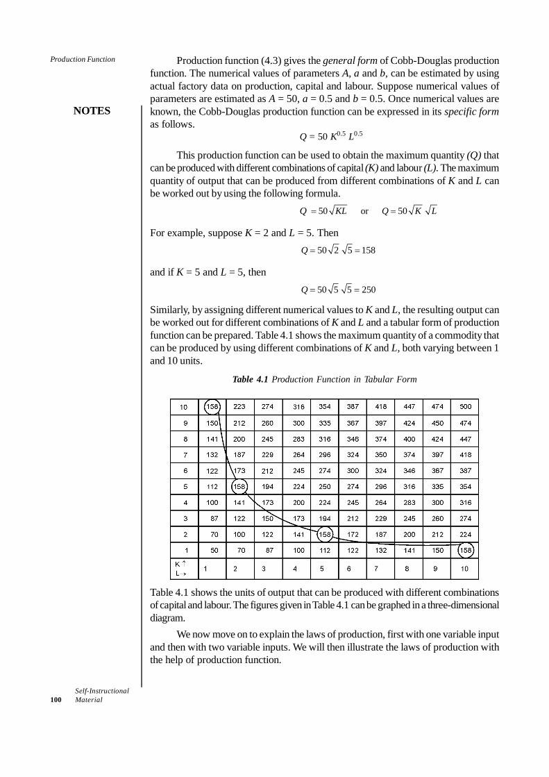
Self-Instructional100 Material
Production Function
NOTES
Production function (4.3) gives the general form of Cobb-Douglas productionfunction. The numerical values of parameters A, a and b, can be estimated by usingactual factory data on production, capital and labour. Suppose numerical values ofparameters are estimated as A = 50, a = 0.5 and b = 0.5. Once numerical values areknown, the Cobb-Douglas production function can be expressed in its specific formas follows.
Q = 50 K0.5 L0.5
This production function can be used to obtain the maximum quantity (Q) thatcan be produced with different combinations of capital (K) and labour (L). The maximumquantity of output that can be produced from different combinations of K and L canbe worked out by using the following formula.
Q 50 or 50KL Q K L= =
For example, suppose K = 2 and L = 5. Then50 2 5 158Q = =
and if K = 5 and L = 5, then50 5 5 250Q = =
Similarly, by assigning different numerical values to K and L, the resulting output canbe worked out for different combinations of K and L and a tabular form of productionfunction can be prepared. Table 4.1 shows the maximum quantity of a commodity thatcan be produced by using different combinations of K and L, both varying between 1and 10 units.
Table 4.1 Production Function in Tabular Form
Table 4.1 shows the units of output that can be produced with different combinationsof capital and labour. The figures given in Table 4.1 can be graphed in a three-dimensionaldiagram.
We now move on to explain the laws of production, first with one variable inputand then with two variable inputs. We will then illustrate the laws of production withthe help of production function.
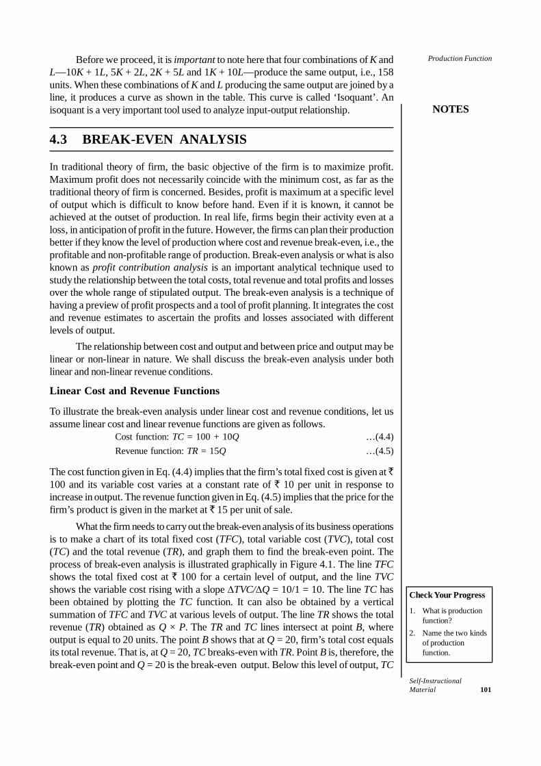
Self-InstructionalMaterial 101
Production Function
NOTES
Before we proceed, it is important to note here that four combinations of K andL—10K + 1L, 5K + 2L, 2K + 5L and 1K + 10L—produce the same output, i.e., 158units. When these combinations of K and L producing the same output are joined by aline, it produces a curve as shown in the table. This curve is called ‘Isoquant’. Anisoquant is a very important tool used to analyze input-output relationship.
4.3 BREAK-EVEN ANALYSIS
In traditional theory of firm, the basic objective of the firm is to maximize profit.Maximum profit does not necessarily coincide with the minimum cost, as far as thetraditional theory of firm is concerned. Besides, profit is maximum at a specific levelof output which is difficult to know before hand. Even if it is known, it cannot beachieved at the outset of production. In real life, firms begin their activity even at aloss, in anticipation of profit in the future. However, the firms can plan their productionbetter if they know the level of production where cost and revenue break-even, i.e., theprofitable and non-profitable range of production. Break-even analysis or what is alsoknown as profit contribution analysis is an important analytical technique used tostudy the relationship between the total costs, total revenue and total profits and lossesover the whole range of stipulated output. The break-even analysis is a technique ofhaving a preview of profit prospects and a tool of profit planning. It integrates the costand revenue estimates to ascertain the profits and losses associated with differentlevels of output.
The relationship between cost and output and between price and output may belinear or non-linear in nature. We shall discuss the break-even analysis under bothlinear and non-linear revenue conditions.
Linear Cost and Revenue Functions
To illustrate the break-even analysis under linear cost and revenue conditions, let usassume linear cost and linear revenue functions are given as follows.
Cost function: TC = 100 + 10Q …(4.4)Revenue function: TR = 15Q …(4.5)
The cost function given in Eq. (4.4) implies that the firm’s total fixed cost is given at ̀100 and its variable cost varies at a constant rate of ` 10 per unit in response toincrease in output. The revenue function given in Eq. (4.5) implies that the price for thefirm’s product is given in the market at ` 15 per unit of sale.
What the firm needs to carry out the break-even analysis of its business operationsis to make a chart of its total fixed cost (TFC), total variable cost (TVC), total cost(TC) and the total revenue (TR), and graph them to find the break-even point. Theprocess of break-even analysis is illustrated graphically in Figure 4.1. The line TFCshows the total fixed cost at ` 100 for a certain level of output, and the line TVCshows the variable cost rising with a slope ΔTVC/ΔQ = 10/1 = 10. The line TC hasbeen obtained by plotting the TC function. It can also be obtained by a verticalsummation of TFC and TVC at various levels of output. The line TR shows the totalrevenue (TR) obtained as Q × P. The TR and TC lines intersect at point B, whereoutput is equal to 20 units. The point B shows that at Q = 20, firm’s total cost equalsits total revenue. That is, at Q = 20, TC breaks-even with TR. Point B is, therefore, thebreak-even point and Q = 20 is the break-even output. Below this level of output, TC
Check Your Progress
1. What is productionfunction?
2. Name the two kindsof productionfunction.
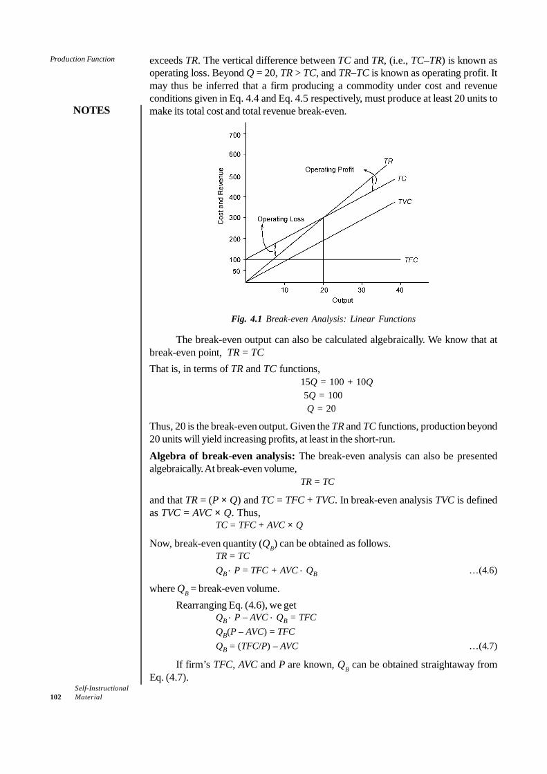
Self-Instructional102 Material
Production Function
NOTES
exceeds TR. The vertical difference between TC and TR, (i.e., TC–TR) is known asoperating loss. Beyond Q = 20, TR > TC, and TR–TC is known as operating profit. Itmay thus be inferred that a firm producing a commodity under cost and revenueconditions given in Eq. 4.4 and Eq. 4.5 respectively, must produce at least 20 units tomake its total cost and total revenue break-even.
Fig. 4.1 Break-even Analysis: Linear Functions
The break-even output can also be calculated algebraically. We know that atbreak-even point, TR = TCThat is, in terms of TR and TC functions,
15Q = 100 + 10Q 5Q = 100 Q = 20
Thus, 20 is the break-even output. Given the TR and TC functions, production beyond20 units will yield increasing profits, at least in the short-run.Algebra of break-even analysis: The break-even analysis can also be presentedalgebraically. At break-even volume,
TR = TC
and that TR = (P × Q) and TC = TFC + TVC. In break-even analysis TVC is definedas TVC = AVC × Q. Thus,
TC = TFC + AVC × Q
Now, break-even quantity (QB) can be obtained as follows.TR = TCQB ⋅ P = TFC + AVC ⋅ QB …(4.6)
where QB = break-even volume.Rearranging Eq. (4.6), we get
QB ⋅ P – AVC ⋅ QB = TFCQB(P – AVC) = TFCQB = (TFC/P) – AVC …(4.7)
If firm’s TFC, AVC and P are known, QB can be obtained straightaway fromEq. (4.7).
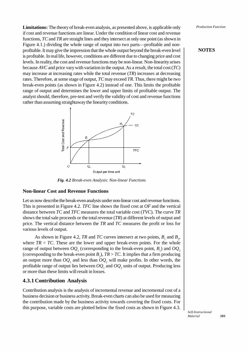
Self-InstructionalMaterial 103
Production Function
NOTES
Limitations: The theory of break-even analysis, as presented above, is applicable onlyif cost and revenue functions are linear. Under the condition of linear cost and revenuefunctions, TC and TR are straight lines and they intersect at only one point (as shown inFigure 4.1.) dividing the whole range of output into two parts—profitable and non-profitable. It may give the impression that the whole output beyond the break-even levelis profitable. In real life, however, conditions are different due to changing price and costlevels. In reality, the cost and revenue functions may be non-linear. Non-linearity arisesbecause AVC and price vary with variation in the output. As a result, the total cost (TC)may increase at increasing rates while the total revenue (TR) increases at decreasingrates. Therefore, at some stage of output, TC may exceed TR. Thus, there might be twobreak-even points (as shown in Figure 4.2) instead of one. This limits the profitablerange of output and determines the lower and upper limits of profitable output. Theanalyst should, therefore, pre-test and verify the validity of cost and revenue functionsrather than assuming straightaway the linearity conditions.
Fig. 4.2 Break-even Analysis: Non-linear Functions
Non-linear Cost and Revenue Functions
Let us now describe the break-even analysis under non-linear cost and revenue functions.This is presented in Figure 4.2. TFC line shows the fixed cost at OF and the verticaldistance between TC and TFC measures the total variable cost (TVC). The curve TRshows the total sale proceeds or the total revenue (TR) at different levels of output andprice. The vertical distance between the TR and TC measures the profit or loss forvarious levels of output.
As shown in Figure 4.2, TR and TC curves intersect at two points, B1 and B2,where TR = TC. These are the lower and upper break-even points. For the wholerange of output between OQ1 (corresponding to the break-even point, B1) and OQ2(corresponding to the break-even point B2), TR > TC. It implies that a firm producingan output more than OQ1 and less than OQ2 will make profits. In other words, theprofitable range of output lies between OQ1 and OQ2 units of output. Producing lessor more than these limits will result in losses.
4.3.1 Contribution Analysis
Contribution analysis is the analysis of incremental revenue and incremental cost of abusiness decision or business activity. Break-even charts can also be used for measuringthe contribution made by the business activity towards covering the fixed costs. Forthis purpose, variable costs are plotted below the fixed costs as shown in Figure 4.3.
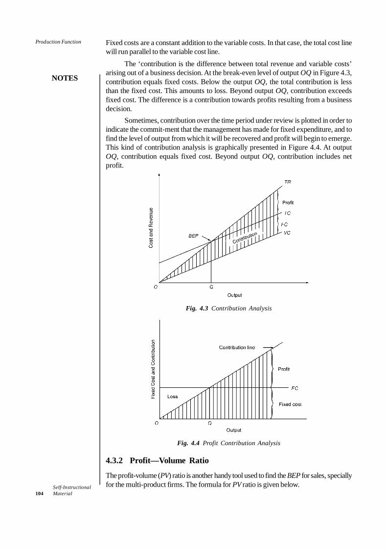
Self-Instructional104 Material
Production Function
NOTES
Fixed costs are a constant addition to the variable costs. In that case, the total cost linewill run parallel to the variable cost line.
The ‘contribution is the difference between total revenue and variable costs’arising out of a business decision. At the break-even level of output OQ in Figure 4.3,contribution equals fixed costs. Below the output OQ, the total contribution is lessthan the fixed cost. This amounts to loss. Beyond output OQ, contribution exceedsfixed cost. The difference is a contribution towards profits resulting from a businessdecision.
Sometimes, contribution over the time period under review is plotted in order toindicate the commit-ment that the management has made for fixed expenditure, and tofind the level of output from which it will be recovered and profit will begin to emerge.This kind of contribution analysis is graphically presented in Figure 4.4. At outputOQ, contribution equals fixed cost. Beyond output OQ, contribution includes netprofit.
Fig. 4.3 Contribution Analysis
Fig. 4.4 Profit Contribution Analysis
4.3.2 Profit—Volume Ratio
The profit-volume (PV) ratio is another handy tool used to find the BEP for sales, speciallyfor the multi-product firms. The formula for PV ratio is given below.
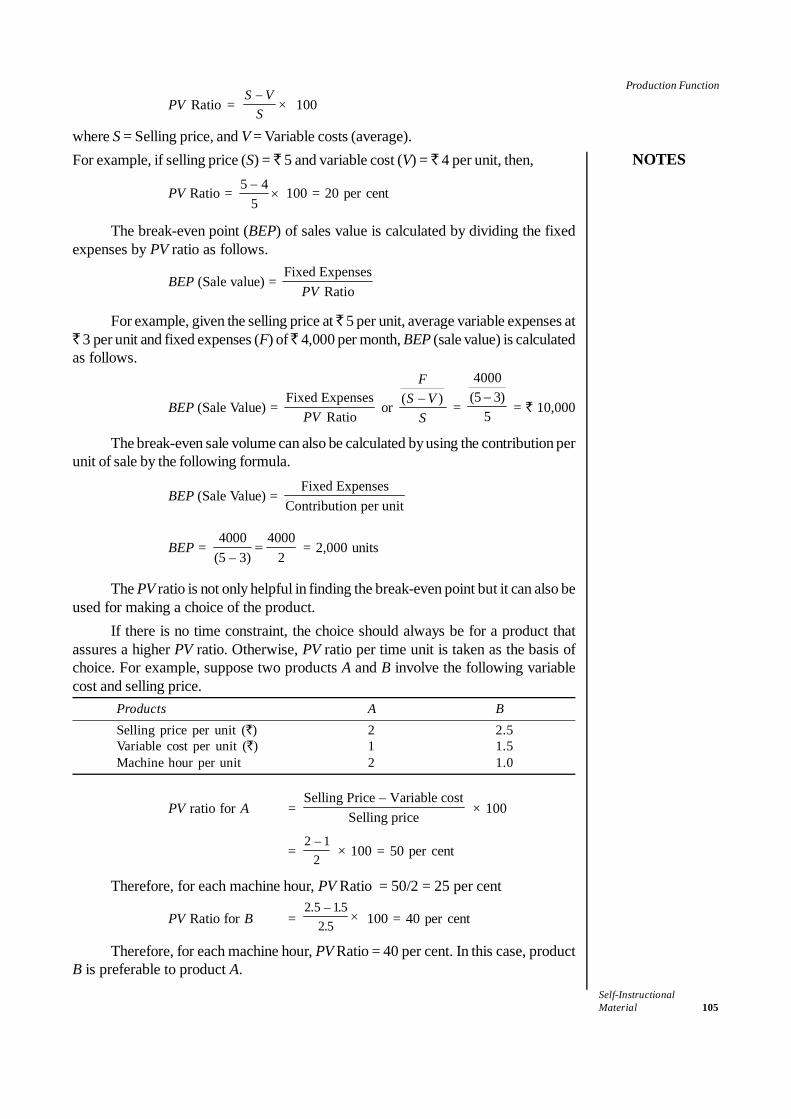
Self-InstructionalMaterial 105
Production Function
NOTES
PV Ratio = S V
S−
× 100
where S = Selling price, and V = Variable costs (average).For example, if selling price (S) = ̀ 5 and variable cost (V) = ̀ 4 per unit, then,
PV Ratio = 5 45−
× 100 = 20 per cent
The break-even point (BEP) of sales value is calculated by dividing the fixedexpenses by PV ratio as follows.
BEP (Sale value) = Fixed Expenses
RatioPV
For example, given the selling price at ̀ 5 per unit, average variable expenses at` 3 per unit and fixed expenses (F) of ̀ 4,000 per month, BEP (sale value) is calculatedas follows.
BEP (Sale Value) = Fixed Expenses
RatioPV or ( )
FS V
S− =
4000(5 3)
5−
= ` 10,000
The break-even sale volume can also be calculated by using the contribution perunit of sale by the following formula.
BEP (Sale Value) = Fixed Expenses
Contribution per unit
BEP = 4000 4000
(5 – 3) 2= = 2,000 units
The PV ratio is not only helpful in finding the break-even point but it can also beused for making a choice of the product.
If there is no time constraint, the choice should always be for a product thatassures a higher PV ratio. Otherwise, PV ratio per time unit is taken as the basis ofchoice. For example, suppose two products A and B involve the following variablecost and selling price.
Products A BSelling price per unit (`) 2 2.5Variable cost per unit (`) 1 1.5Machine hour per unit 2 1.0
PV ratio for A = Selling Price – Variable cost
Selling price × 100
= 2 – 1
2 × 100 = 50 per cent
Therefore, for each machine hour, PV Ratio = 50/2 = 25 per cent
PV Ratio for B = 2.5 – 1.5
2.5× 100 = 40 per cent
Therefore, for each machine hour, PV Ratio = 40 per cent. In this case, productB is preferable to product A.
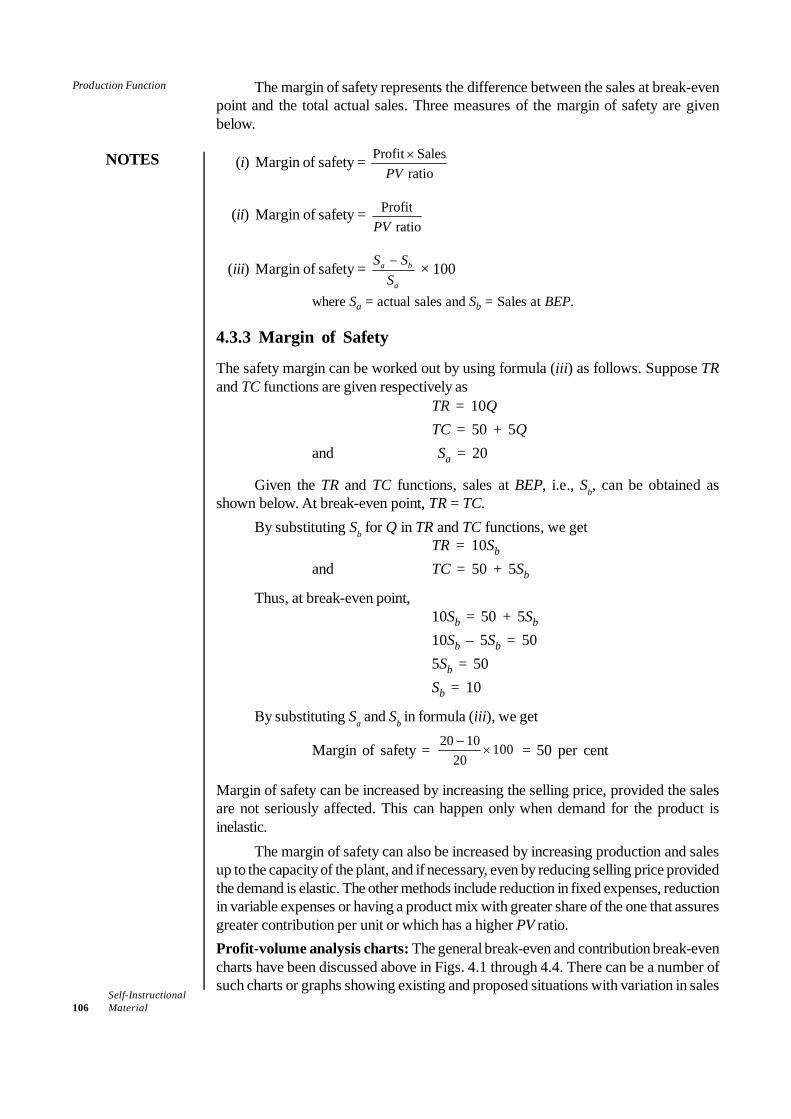
Self-Instructional106 Material
Production Function
NOTES
The margin of safety represents the difference between the sales at break-evenpoint and the total actual sales. Three measures of the margin of safety are givenbelow.
(i) Margin of safety = Profit SalesratioPV×
(ii) Margin of safety = ProfitratioPV
(iii) Margin of safety = a b
a
S SS− × 100
where Sa = actual sales and Sb = Sales at BEP.
4.3.3 Margin of Safety
The safety margin can be worked out by using formula (iii) as follows. Suppose TRand TC functions are given respectively as
TR = 10QTC = 50 + 5Q
and Sa = 20
Given the TR and TC functions, sales at BEP, i.e., Sb, can be obtained asshown below. At break-even point, TR = TC.
By substituting Sb for Q in TR and TC functions, we getTR = 10Sb
and TC = 50 + 5Sb
Thus, at break-even point,10Sb = 50 + 5Sb
10Sb – 5Sb = 505Sb = 50Sb = 10
By substituting Sa and Sb in formula (iii), we get
Margin of safety = 20 10 100
20−
× = 50 per cent
Margin of safety can be increased by increasing the selling price, provided the salesare not seriously affected. This can happen only when demand for the product isinelastic.
The margin of safety can also be increased by increasing production and salesup to the capacity of the plant, and if necessary, even by reducing selling price providedthe demand is elastic. The other methods include reduction in fixed expenses, reductionin variable expenses or having a product mix with greater share of the one that assuresgreater contribution per unit or which has a higher PV ratio.Profit-volume analysis charts: The general break-even and contribution break-evencharts have been discussed above in Figs. 4.1 through 4.4. There can be a number ofsuch charts or graphs showing existing and proposed situations with variation in sales

Self-InstructionalMaterial 107
Production Function
NOTES
price, fixed and variable cost and, consequently, variable contributions to fixed costs,profits. One of such charts is the cash break-even chart.
A cash break-even chart can be prepared by taking cash inflow from sales andcash outlay on fixed and variable costs. The distribution of the total contribution mayalso be shown from the angle of incidence as shown in Figure 4.5.
Another variation of the break-even chart is called profit-volume analysis chartor graph. In this chart, the horizontal axis represents the sales volume and the verticalaxis shows profit or loss. The profit line is graphed by computing the profit or lossconsisting of the difference between sales revenue and the total cost at each volume.The point where the profit line intersects the horizontal axis is the break-even point.This has been shown in Figure 4.6.
It may be noticed that break-even charts are good for displaying information.The same information is available from simple calculations.
Fig. 4.5 Cash Break-Even Analysis
Fig. 4.6 Profit Volume Analysis
Check Your Progress
3. What is a breakevenanalysis?
4. Define contributionanalysis.
5. What is a profit-volume analysischart?
6. Break-even analysisis an importantanalytical techniqueused to:
(a) Study therelationshipbetween thetotal costs, totalrevenue and totalprofits andlosses over thewhole range ofstipulatedoutput
(b) Study themathematicalpresentation ofinput-outputrelationship
(c) Measure supplyof capital in ashort-run period
(d) Analyse theincrementalrevenue andincremental costof a businessdecision oractivity
Self-Instructional108 Material
Production Function
NOTES
Use of Break-Even Analysis
• Sales volume can be determined to earn a given amount of return on capital• Profit can be forecast if estimates of revenue and cost are available• Effect of change in the volume of sales, sale price, cost of production, can be
appraised• Choice of products can be made from the alternatives available. Product-mix can
also be determined• Impact of increase or decrease in fixed and variable costs can be highlighted• Effect of high fixed costs and low variable costs to the total cost can be studied• Valid inter-firm comparisons of profitability can be made• Cash break-even chart helps proper planning of cash requirements• Break-even analysis emphasizes the importance of capacity utilization for
achieving economies• Further help is provided by margin of safety and angle of incidence
We have discussed above that the break-even analysis is based on linear assumptions.The linearity assumption can be removed by pre-testing the cost and revenue functionsand by using, if necessary, the non-linearity conditions. Nevertheless, the break-evenanalysis as such has certain other limitations.
First, the break-even analysis can be applied only to a single product system.Under the condition of multiple products and joint operations, the break-even analysiscan be applied only if product-wise cost can be ascertained which is, of course,extremely difficult.
Second, break-even analysis cannot be applied usefully where cost and pricedata cannot be ascertained beforehand and where historical data are not relevant forestimating future costs and prices. Despite these limitations, the break-even analysismay serve a useful purpose in production planning if relevant data can be easily obtained.
4.4 LAW OF VARIABLE PROPORTION
The laws of production state the relationship between output and input. In the short-run, input-output relations are studied with one variable input (labour), other inputs(especially, capital) held constant. The laws of production under these conditions arecalled the ‘Laws of Variable Proportions’ or the ‘Laws of Returns to a Variable Input’.In this section, we explain the ‘laws of returns to a variable input’.
Law of Diminishing Returns to a Variable Input
Law of Diminishing Returns: The law of diminishing returns states that when moreand more units of a variable input are used with a given quantity of fixed inputs, thetotal output may initially increase at increasing rate and then at a constant rate, butit will eventually increase at diminishing rates. That is, the marginal increase in totaloutput decreases eventually when additional units of a variable factor are used, givenquantity of fixed factors.
Check Your Progress
7. State whichsentence is incorrect
(a) Break-evencharts are goodfor displayinginformationcollected fromsimplecalculations
(b) Break-evenanalysis can beapplied only to asingle productsystem
(c) Break-evenanalysis cannotserve a usefulpurpose inproductionplanning ifrelevant data canbe easilyobtained
(d) Break-evenanalysis cannotbe appliedusefully wherecost and pricedata cannot beascertainedbeforehand andwhere historicaldata are notrelevant forestimating futurecosts and prices

Self-InstructionalMaterial 109
Production Function
NOTES
Assumptions: The law of diminishing returns is based on the following assumptions:(i) Labour is the only variable input, capital remaining constant(ii) Labour is homogeneous
(iii) The state of technology is given(iv) Input prices are given
To illustrate the law of diminishing returns, let us assume (i) that a firm (say, the coalmining firm in our earlier example) has a set of mining machinery as its capital (K) fixedin the short-run, and (ii) that it can employ only more mine-workers to increase its coalproduction. Thus, the short-run production function for the firm will take the followingform.
Qc = f(L), K constant
Let us assume also that the labour-output relationship in coal production is givenby a hypothetical production function of the following form.
Qc = – L3 + 15L2 + 10L …(4.8)
Given the production function (4.8), we may substitute different numerical valuesfor L in the function and work out a series of Qc, i.e., the quantity of coal that can beproduced with different number of workers. For example, if L = 5, then by substitution,we get
Qc = – 53 + 15 × 52 + 10 × 5 = – 125 + 375 + 50 = 300
A tabular array of output levels associated with different number of workersfrom 1 to 12, in our hypothetical coal-production example, is given in Table 4.2 (Cols.1 and 2).
What we need now is to work out marginal productivity of labour (MPL) tofind the trend in the contribution of the marginal labour and average productivity oflabour (APL) to find the average contribution of labour.Marginal Productivity of Labour (MPL) can be obtained by differentiating theproduction function (4.8). Thus,
MPL = LQ
∂∂ = – 3L2 + 30L + 10 …(4.9)
By substituting numerical value for labour (L) in Eq. (4.9), MPL can be obtained atdifferent levels of labour employment. However, this method can be used only wherelabour is perfectly divisible and ∂L → 0. Since, in our example, each unit of L = 1,calculus method cannot be used.
Alternatively, where labour can be increased at least by one unit, MPL can beobtained as
MPL = TPL – TPL–1
The MPL worked out by this method is presented in Col. 3 of Table 4.2.Average productivity of labour (APL) can be obtained by dividing the production functionby L. Thus,
APL = 3 215 10L L L
L− + +
= –L2 + 15L + 10 ...(4.10)

Self-Instructional110 Material
Production Function
NOTES
Now APL can be obtained by substituting the numerical value for L in Eq. (4.10). APLobtained by this method is given in Col. 4 of Table 4.2.
Tables 4.2 Three Stages of Production
No. of Workers Total Product Marginal Average Stages of(N) (TPL) Product* Product Production
(tonnes) (MPL) (APL) (based on MPL)
(1) (2) (3) (4) (5)1 24 24 24 I2 72 48 36 Increasing3 138 66 46 returns4 216 78 545 300 84 606 384 84 647 462 78 66 II8 528 66 66 Diminishing9 576 48 64 returns10 600 24 6011 594 – 6 54 III12 552 – 42 46 Negative returns
*MPL = TPn – TPn–1. MPL calculated by differential method will be different from that given in Col.3.The information contained in Table 4.2 is presented graphically in panels (a) and (b) ofFigure 4.7. Panel (a) of Figure 7.7 presents the total product curve (TPL) and panel (b)presents marginal product (MPL) and average product (APL) curves. The TPL scheduledemonstrates the law of diminishing returns. As the curve TPL shows, the total outputincreases at an increasing rate till the employment of the 5th worker, as indicated by theincreasing slope of the TPL curve. (See also Col. 3 of the table). Employment of the 6thworker contributes as much as the 5th worker. Note that beyond the employment of the6th worker, although TPL continues to increase (until the 10th worker), the rate of increasein TPL (i.e., MPL) begins to fall. This shows the operation of the law of diminishingreturns.The three stages in production: Table 4.2 and Figure 4.7 present the three usualstages in the application of the laws of diminishing returns.
In Stage I, TPL increases at increasing rate. This is indicated by the rising MPL tillthe employment of the 5th and 6th workers. Given the production function (4.8), the 6thworker produces as much as the 5th worker. The output from the 5th and the 6thworkers represents an intermediate stage of constant returns to the variable factor,labour.

Self-InstructionalMaterial 111
Production Function
NOTES
Fig. 4.7 Total, Average and Marginal Products
In Stage II, TPL continues to increase but at diminishing rates, i.e., MPL begins todecline. This stage in production shows the law of diminishing returns to the variablefactor. Total output reaches its maximum level at the employment of the 10th worker.Beyond this level of labour employment, TPL begins to decline. This marks the beginningof Stage III in production.
To conclude, the law of diminishing returns can be stated as follows. Giventhe employment of the fixed factor (capital), when more and more workers are employed,the return from the additional worker may initially increase but will eventually decrease.Factors behind the laws of returns: As shown in Figure 4.7, the marginal productivityof labour (MPL) increases is Stage I, whereas it decreases in Stage II. In other words,in Stage I, Law of Increasing Returns is in operation and in Stage II, the law ofDiminishing Returns is in application. The reasons which underly the application of thelaws of returns in Stages I and II may be described as follows.
One of the important factors causing increasing returns to a variable factor isthe indivisibility of fixed factor (capital). The minimum size of capital is given as itcannot be divided to suit the number of workers. Therefore, if labour is less than itsoptimum number, capital remains underutilized. Let us suppose that optimum capital-labour combination is 1:6. If capital is indivisible and less than 6 workers are employed,then capital would remain underutilized. When more and more workers are added,utilization of capital increases and also the productivity of additional worker. Thesecond and the most important reason for increase in labour productivity is the divisionof labour that becomes possible with the employment of additional labour, untiloptimum capital-labour combination is reached.
Self-Instructional112 Material
Production Function
NOTES
Once the optimum capital-labour ratio is reached, employment of additional workersamounts to substitution of capital with labour. But, technically, there is a limit to whichone input can be substituted for another. That is, labour cannot substitute for capitalbeyond a limit. Hence, to replace the same amount of capital, more and more workerswill have to be employed because per worker marginal productivity decreases. Also,with increasing number of workers, capital remaining the same, capital-labour ratio goeson decreasing. As a result, productivity of labour begins to decline. This marks thebeginning of the second stage.
Application of the Law of Diminishing Returns
The law of diminishing returns is an empirical law, frequently observed in variousproduction activities. This law, however, may not apply universally to all kinds ofproductive activities since it is not as true as the law of gravitation. In some productiveactivities, it may operate quickly, in some its operation may take a little longer time andin some others, it may not appear at all. This law has been found to operate in agriculturalproduction more regularly than in industrial production. The reason is, in agriculture,natural factors play a predominant role whereas man-made factors play the major rolein industrial production. Despite the limitations of the law, if increasing units of aninput are applied to the fixed factors, the marginal returns to the variable input decreaseeventually.Law of diminishing returns and business decisions: The law of diminishing returnsas presented graphically has a relevance to the business decisions. The graph can helpin identifying the rational and irrational stages of operations. It can also tell the businessmanagers the number of workers (or other variable inputs) to apply to a given fixedinput so that, given all other factors, output is maximum. As Figure 4.7 exhibits, capitalis presumably underutilized in Stage I. So a firm operating in Stage I is required toincrease labour, and a firm operating in Stage III is required to reduce labour, with aview to maximizing its total production. From the firm’s point of view, setting anoutput target in Stages I and III is irrational. The only meaningful and rational stagefrom the firm’s point of view is Stage II in which the firm can find answer to thequestion ‘how many workers to employ’. Figure 4.7 shows that the firm should employa minimum of 7 workers and a maximum of 10 workers even if labour is available freeof cost. This means that the firm has a limited choice—ranging from 7 to 10 workers.How many workers to employ against the fixed capital and how much to produce canbe answered, only when the price of labour, i.e., wage rate, and that of the product areknown. This question is answered below.
4.4.1 Determining Optimum Employment of Labour
It may be recalled from Figure 4.7 that an output maximizing coal-mining firm wouldlike to employ 10 workers since at this level of employment, the output is maximum.The firm can, however, employ 10 workers only if workers are available free of cost.But labour is not available free of cost—the firm is required to pay wages to theworkers. Therefore, the question arises as to how many workers will the firm employ—10 or less or more than 10—to maximize its profit. A simple answer to this question isthat the number of workers to be employed depends on the output that maximizes thefirm’s profit, given the product price and the wage rate. This point can be proved asfollows.We know that profit is maximum where
MC = MR
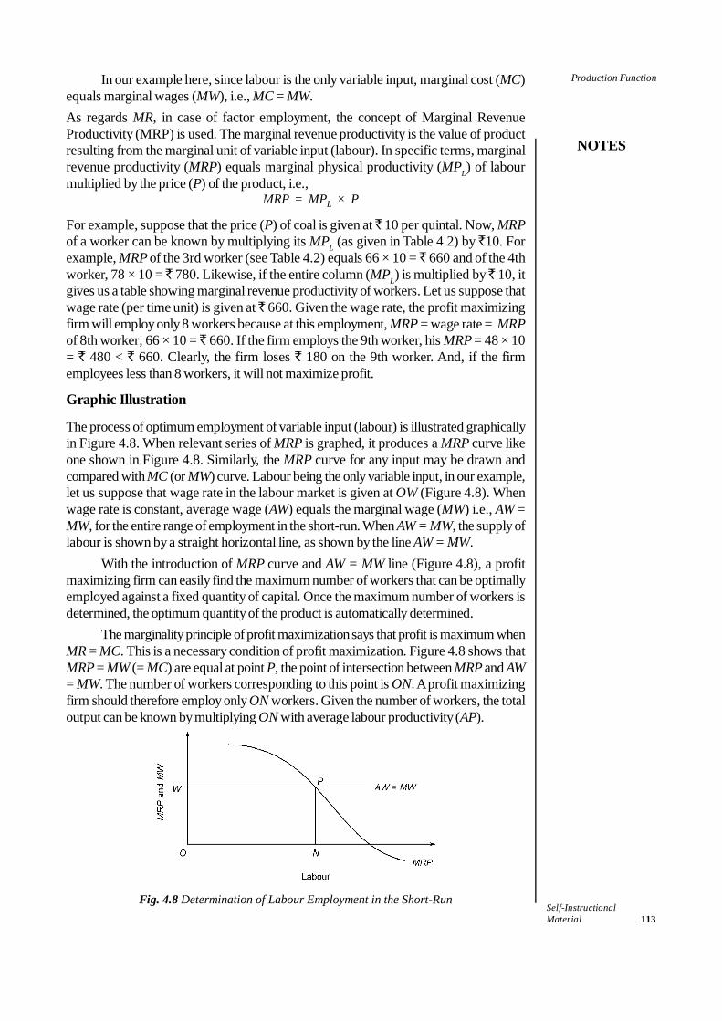
Self-InstructionalMaterial 113
Production Function
NOTES
In our example here, since labour is the only variable input, marginal cost (MC)equals marginal wages (MW), i.e., MC = MW.As regards MR, in case of factor employment, the concept of Marginal RevenueProductivity (MRP) is used. The marginal revenue productivity is the value of productresulting from the marginal unit of variable input (labour). In specific terms, marginalrevenue productivity (MRP) equals marginal physical productivity (MPL) of labourmultiplied by the price (P) of the product, i.e.,
MRP = MPL × P
For example, suppose that the price (P) of coal is given at ̀ 10 per quintal. Now, MRPof a worker can be known by multiplying its MPL (as given in Table 4.2) by `10. Forexample, MRP of the 3rd worker (see Table 4.2) equals 66 × 10 = ̀ 660 and of the 4thworker, 78 × 10 = ̀ 780. Likewise, if the entire column (MPL) is multiplied by ̀ 10, itgives us a table showing marginal revenue productivity of workers. Let us suppose thatwage rate (per time unit) is given at ̀ 660. Given the wage rate, the profit maximizingfirm will employ only 8 workers because at this employment, MRP = wage rate = MRPof 8th worker; 66 × 10 = ̀ 660. If the firm employs the 9th worker, his MRP = 48 × 10= ` 480 < ` 660. Clearly, the firm loses ` 180 on the 9th worker. And, if the firmemployees less than 8 workers, it will not maximize profit.
Graphic Illustration
The process of optimum employment of variable input (labour) is illustrated graphicallyin Figure 4.8. When relevant series of MRP is graphed, it produces a MRP curve likeone shown in Figure 4.8. Similarly, the MRP curve for any input may be drawn andcompared with MC (or MW) curve. Labour being the only variable input, in our example,let us suppose that wage rate in the labour market is given at OW (Figure 4.8). Whenwage rate is constant, average wage (AW) equals the marginal wage (MW) i.e., AW =MW, for the entire range of employment in the short-run. When AW = MW, the supply oflabour is shown by a straight horizontal line, as shown by the line AW = MW.
With the introduction of MRP curve and AW = MW line (Figure 4.8), a profitmaximizing firm can easily find the maximum number of workers that can be optimallyemployed against a fixed quantity of capital. Once the maximum number of workers isdetermined, the optimum quantity of the product is automatically determined.
The marginality principle of profit maximization says that profit is maximum whenMR = MC. This is a necessary condition of profit maximization. Figure 4.8 shows thatMRP = MW (= MC) are equal at point P, the point of intersection between MRP and AW= MW. The number of workers corresponding to this point is ON. A profit maximizingfirm should therefore employ only ON workers. Given the number of workers, the totaloutput can be known by multiplying ON with average labour productivity (AP).
Fig. 4.8 Determination of Labour Employment in the Short-Run
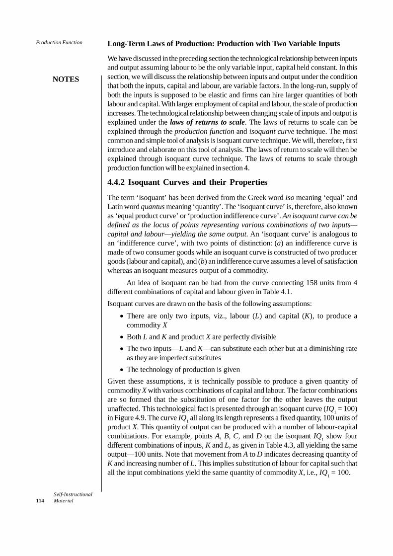
Self-Instructional114 Material
Production Function
NOTES
Long-Term Laws of Production: Production with Two Variable Inputs
We have discussed in the preceding section the technological relationship between inputsand output assuming labour to be the only variable input, capital held constant. In thissection, we will discuss the relationship between inputs and output under the conditionthat both the inputs, capital and labour, are variable factors. In the long-run, supply ofboth the inputs is supposed to be elastic and firms can hire larger quantities of bothlabour and capital. With larger employment of capital and labour, the scale of productionincreases. The technological relationship between changing scale of inputs and output isexplained under the laws of returns to scale. The laws of returns to scale can beexplained through the production function and isoquant curve technique. The mostcommon and simple tool of analysis is isoquant curve technique. We will, therefore, firstintroduce and elaborate on this tool of analysis. The laws of return to scale will then beexplained through isoquant curve technique. The laws of returns to scale throughproduction function will be explained in section 4.
4.4.2 Isoquant Curves and their Properties
The term ‘isoquant’ has been derived from the Greek word iso meaning ‘equal’ andLatin word quantus meaning ‘quantity’. The ‘isoquant curve’ is, therefore, also knownas ‘equal product curve’ or ‘production indifference curve’. An isoquant curve can bedefined as the locus of points representing various combinations of two inputs—capital and labour—yielding the same output. An ‘isoquant curve’ is analogous toan ‘indifference curve’, with two points of distinction: (a) an indifference curve ismade of two consumer goods while an isoquant curve is constructed of two producergoods (labour and capital), and (b) an indifference curve assumes a level of satisfactionwhereas an isoquant measures output of a commodity.
An idea of isoquant can be had from the curve connecting 158 units from 4different combinations of capital and labour given in Table 4.1.Isoquant curves are drawn on the basis of the following assumptions:
• There are only two inputs, viz., labour (L) and capital (K), to produce acommodity X
• Both L and K and product X are perfectly divisible• The two inputs—L and K—can substitute each other but at a diminishing rate
as they are imperfect substitutes• The technology of production is given
Given these assumptions, it is technically possible to produce a given quantity ofcommodity X with various combinations of capital and labour. The factor combinationsare so formed that the substitution of one factor for the other leaves the outputunaffected. This technological fact is presented through an isoquant curve (IQ1 = 100)in Figure 4.9. The curve IQ1 all along its length represents a fixed quantity, 100 units ofproduct X. This quantity of output can be produced with a number of labour-capitalcombinations. For example, points A, B, C, and D on the isoquant IQ1 show fourdifferent combinations of inputs, K and L, as given in Table 4.3, all yielding the sameoutput—100 units. Note that movement from A to D indicates decreasing quantity ofK and increasing number of L. This implies substitution of labour for capital such thatall the input combinations yield the same quantity of commodity X, i.e., IQ1 = 100.

Self-InstructionalMaterial 115
Production Function
NOTES
Fig. 4.9 Isoquant Curves
Table 4.3 Capital Labour Combinations and Output
Points Input CombinationsOutputK + L
A OK4 + OL1 = 100B OK3 + OL2 = 100C OK2 + OL3 = 100D OK1 + OL4 = 100
Properties of Isoquant Curves
Isoquants, i.e., production indifference curves, have the same properties as consumer’sindifference curves. Properties of isoquants are explained below in terms of inputs andoutput.
(a) Isoquants have a negative slope: An isoquant has a negative slope in theeconomic region4 and in the economic range of isoquant. The economic regionis the region on the production plane and economic range of isoquant is the rangein which substitution between inputs is technically feasible. Economic region isalso known as the product maximizing region. The negative slope of the isoquantimplies substitutability between the inputs. It means that if one of the inputs isreduced, the other input has to be so increased that the total output remainsunaffected. For example, movement from A to B on IQ1 (Figure 4.9) means thatif K4 K3 units of capital are removed from the production process, L1L2 units oflabour have to be brought in to maintain the same level of output.
(b) Isoquants are convex to the origin: Convexity of isoquants implies two things:(i) substitution between the two inputs, and (ii) diminishing marginal rate oftechnical substitution (MRTS) between the inputs in the economic region. TheMRTS is defined as
MRTS = KL
−ΔΔ
= slope of the isoquant
In plain words, MRTS is the rate at which a marginal unit of labour can substitutea marginal unit of capital (moving downward on the isoquant) without affectingthe total output. This rate is indicated by the slope of the isoquant. The MRTSdecreases for two reasons: (i) no factor is a perfect substitute for another, and

Self-Instructional116 Material
Production Function
NOTES
(ii) inputs are subject to diminishing marginal returns. Therefore, more and moreunits of an input are needed to replace each successive unit of the other input. Forexample, suppose various units of K (minus sign ignored) in Figure 4.9 are equal,i.e.,
ΔK1 = ΔK2 = ΔK3
the corresponding units of L substituting K go (in Figure 4.9) on increasing, i.e.,ΔL1 < ΔL2 < ΔL3
As a result, MRTS = ΔK/ΔL goes on decreasing, i.e.,
3
3
2
2
1
1LK
LK
LK
ΔΔ
>ΔΔ
>ΔΔ
(c) Isoquants are non-intersecting and non-tangential: The intersection ortangency between any two isoquants implies that a given quantity of a commoditycan be produced with a smaller as well as a larger input-combination. This isuntenable so long as marginal productivity of inputs is greater than zero. Thispoint can be proved graphically. Note that in Figure 4.10, two isoquants intersecteach other at point M. Consider two other points—point J on isoquant marked Q1= 100 and point K on isoquant marked Q2 = 200 such that points K and J fall on avertical line KL2, denoting the same amount of labour (OL2) but different units ofcapital—KL2 units of capital at point K and JL2 units of capital at point J. Notethat point M is common to both the isoquants. Given the definition of isoquant, onecan easily infer that a quantity that can be produced with the combination of Kand L at point M can be produced also with factor combination at points J and K.On the isoquant Q1 = 100, factor combinations at points M and J yield 100 units ofoutput. And, on the isoquant Q2 = 200, factor combinations at M and K yield 200units of output. Since point M is common to both the isoquants, it follows thatinput combinations at J and K are equal in terms of output. This implies that interms of output,
OL2(L) + JL2(K) = OL2(L) + KL2(K)
Since OL2 is common to both the sides, it means, JL2(K) = KL2(K)
But it can be seen in Figure 4.10 thatJL2(K) < KL2(K)
But the intersection of the two isoquants means that JL2 and KL2 are equal interms of their output. This is wrong. That is why isoquants will not intersect or betangent to each other. If they do, it violates the laws of production.
Fig. 4.10 Intersecting Isoquants
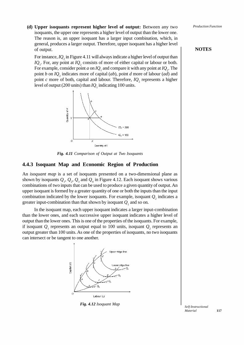
Self-InstructionalMaterial 117
Production Function
NOTES
(d) Upper isoquants represent higher level of output: Between any twoisoquants, the upper one represents a higher level of output than the lower one.The reason is, an upper isoquant has a larger input combination, which, ingeneral, produces a larger output. Therefore, upper isoquant has a higher levelof output.For instance, IQ2 in Figure 4.11 will always indicate a higher level of output thanIQ1. For, any point at IQ2 consists of more of either capital or labour or both.For example, consider point a on IQ1 and compare it with any point at IQ2. Thepoint b on IQ2 indicates more of capital (ab), point d more of labour (ad) andpoint c more of both, capital and labour. Therefore, IQ2 represents a higherlevel of output (200 units) than IQ1 indicating 100 units.
Fig. 4.11 Comparison of Output at Two Isoquants
4.4.3 Isoquant Map and Economic Region of Production
An isoquant map is a set of isoquants presented on a two-dimensional plane asshown by isoquants Q1, Q2, Q3 and Q4 in Figure 4.12. Each isoquant shows variouscombinations of two inputs that can be used to produce a given quantity of output. Anupper isoquant is formed by a greater quantity of one or both the inputs than the inputcombination indicated by the lower isoquants. For example, isoquant Q2 indicates agreater input-combination than that shown by isoquant Q1 and so on.
In the isoquant map, each upper isoquant indicates a larger input-combinationthan the lower ones, and each successive upper isoquant indicates a higher level ofoutput than the lower ones. This is one of the properties of the isoquants. For example,if isoquant Q1 represents an output equal to 100 units, isoquant Q2 represents anoutput greater than 100 units. As one of the properties of isoquants, no two isoquantscan intersect or be tangent to one another.
Fig. 4.12 Isoquant Map

Self-Instructional118 Material
Production Function
NOTES
Economic region: Economic region is that area of production plane in which substitutionbetween two inputs is technically feasible without affecting the output. This area ismarked by locating the points on the isoquants at which MRTS = 0. A zero MRTSimplies that further substitution between inputs is technically not feasible. It alsodetermines the minimum quantity of an input that must be used to produce a givenoutput. Beyond this point, an additional employment of one input will necessitateemploying additional units of the other input. Such a point on an isoquant may beobtained by drawing a tangent to the isoquant and parallel to the vertical and horizontalaxes, as shown by dashed lines in Figure 4.12. By joining the resulting points a, b, cand d, we get a line called the upper ridge line, Od. Similarly, by joining the points e,f, g and h, we get the lower ridge line, Oh. The ridge lines are locus of points on theisoquants where the marginal products (MP) of the inputs are equal to zero. The upperridge line implies that MP of capital is zero along the line, Od. The lower ridge lineimplies that MP of labour is zero along the line, Oh.
The area between the two ridge lines, Od and Oh, is called ‘Economic Region’or ‘technically efficient region’ of production. Any production technique, i.e., capital-labour combination, within the economic region is technically efficient to produce agiven output. And, any production technique outside this region is technically inefficientsince it requires more of both inputs to produce the same quantity of output.
Other Forms of Isoquants
We have introduced above a convex isoquant that is most widely used in traditionaleconomic theory. The shape of an isoquant, however, depends on the degree ofsubstitutability between the factors in the production function. The convex isoquantpresented in Figure 4.9 assumes a continuous substitutability between capital andlabour but at a diminishing rate. The economists have, however, observed other degreesof substitutability between K and L and have demonstrated the existence of three otherkinds of isoquants.1. Linear isoquants: A linear isoquant is presented by the line AB in Figure 4.13. Alinear isoquant implies perfect substitutability between the two inputs, K and L. Theisoquant AB indicates that a given quantity of a product can be produced by usingonly capital or only labour or by using both. This is possible only when the twofactors, K and L, are perfect substitutes for one another. A linear isoquant also impliesthat the MRTS between K and L remains constant throughout.
The mathematical form of the production function exhibiting perfectsubstitutability of factors is given as follows.
If Q = f(K, L) then, = aK + bL ...(4.11)
The production function (4.11) means that the total output, Q, is simply theweighted sum of K and L. The slope of the resulting isoquant from this productionfunction is given by – b/a. This can be proved as shown below.Given the production function (4.11),
MPK = Q aK
∂=
∂and MPL =
Q bL
∂=
∂
Since MRTS = L
K
MPMP and L
K
MP bMP a
−=
Therefore, MRTS = ba
− = slope of the isoquant

Self-InstructionalMaterial 119
Production Function
NOTES
The production function exhibiting perfect substitutability of factors is, however,unlikely to exist in the real world production process.
Fig. 4.13 Linear Isoquant
2. Isoquants with fixed factor-proportion or L-shaped isoquants: When aproduction function assumes a fixed proportion between K and L, the isoquant takes‘L’ shape, as shown by isoquants Q1 and Q2 in Figure 4.14. Such an isoquant implieszero substitutability between K and L. Instead, it assumes perfect complementaritybetween K and L. The perfect complementarity assumption implies that a given quantityof a commodity can be produced by one and only one combination of K and L andthat the proportion of the inputs is fixed. It also implies that if the quantity of an inputis increased and the quantity of the other input is held constant, there will be no changein output. The output can be increased only by increasing both the inputs proportionately.
As shown in Figure 4.14, to produce Q1 quantity of a product, OK1 units of Kand OL1 units of L are required. It means that if OK1 units of K are being used, OL1units of labour must be used to produce Q1 units of a commodity. Similarly, if OL1units of labour are employed, OK1 units of capital must be used to produce Q1. Ifunits of only K or only L are increased, output will not increase. If output is to beincreased to Q2, K has to be increased by K1K2 and labour by L1L2. This kind oftechnological relationship between K and L gives a fixed proportion production function.A fixed-proportion production function, called Leontief function, is given as
Q = f(K, L) = min (aK, bL) …(4.12)
where ‘min’ means that Q equals the lower of the two terms, aK and bL. That is, if aK> bL, Q = bL and if bL > aK, then Q = aK. If aK = bL, it would mean that both K andL are fully employed. Then the fixed capital labour ratio will be K/L = b/a.
In contrast to a linear production function, the fixed-factor-proportion productionfunction has a wide range of application in the real world. One can find many techniquesof production in which a fixed proportion of labour and capital is fixed. For example,to run a taxi or to operate a photocopier, one needs only one labour. In these cases,the machine-labour proportion is fixed. Any extra labour would be redundant. Similarly,one can find cases in manufacturing industries where capital-labour proportions arefixed.3. Kinked isoquants or linear programming isoquants: The fixed proportionproduction function (Figure 4.14) assumes that there is only one technique of production,and capital and labour can be combined only in a fixed proportion. It implies that to
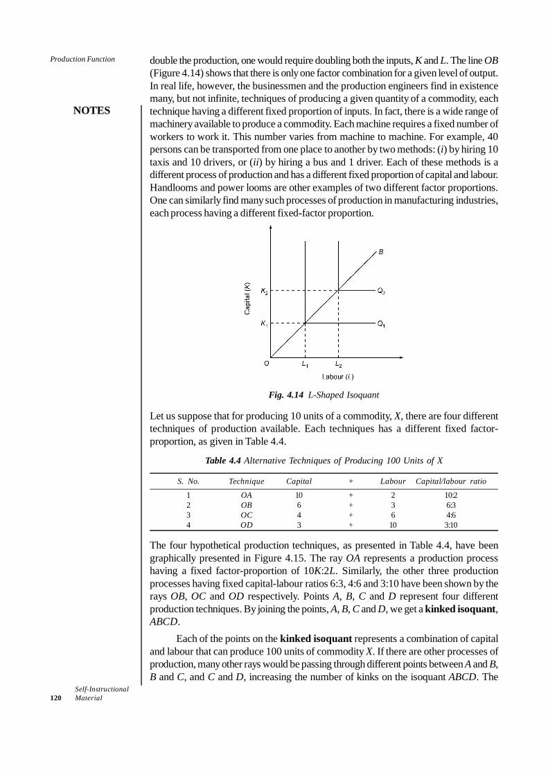
Self-Instructional120 Material
Production Function
NOTES
double the production, one would require doubling both the inputs, K and L. The line OB(Figure 4.14) shows that there is only one factor combination for a given level of output.In real life, however, the businessmen and the production engineers find in existencemany, but not infinite, techniques of producing a given quantity of a commodity, eachtechnique having a different fixed proportion of inputs. In fact, there is a wide range ofmachinery available to produce a commodity. Each machine requires a fixed number ofworkers to work it. This number varies from machine to machine. For example, 40persons can be transported from one place to another by two methods: (i) by hiring 10taxis and 10 drivers, or (ii) by hiring a bus and 1 driver. Each of these methods is adifferent process of production and has a different fixed proportion of capital and labour.Handlooms and power looms are other examples of two different factor proportions.One can similarly find many such processes of production in manufacturing industries,each process having a different fixed-factor proportion.
Fig. 4.14 L-Shaped Isoquant
Let us suppose that for producing 10 units of a commodity, X, there are four differenttechniques of production available. Each techniques has a different fixed factor-proportion, as given in Table 4.4.
Table 4.4 Alternative Techniques of Producing 100 Units of X
S. No. Technique Capital + Labour Capital/labour ratio
1 OA 10 + 2 10:22 OB 6 + 3 6:33 OC 4 + 6 4:64 OD 3 + 10 3:10
The four hypothetical production techniques, as presented in Table 4.4, have beengraphically presented in Figure 4.15. The ray OA represents a production processhaving a fixed factor-proportion of 10K:2L. Similarly, the other three productionprocesses having fixed capital-labour ratios 6:3, 4:6 and 3:10 have been shown by therays OB, OC and OD respectively. Points A, B, C and D represent four differentproduction techniques. By joining the points, A, B, C and D, we get a kinked isoquant,ABCD.
Each of the points on the kinked isoquant represents a combination of capitaland labour that can produce 100 units of commodity X. If there are other processes ofproduction, many other rays would be passing through different points between A and B,B and C, and C and D, increasing the number of kinks on the isoquant ABCD. The
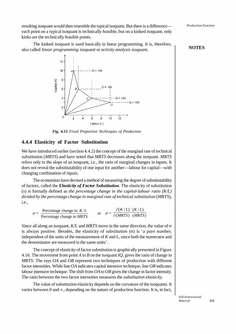
Self-InstructionalMaterial 121
Production Function
NOTES
resulting isoquant would then resemble the typical isoquant. But there is a difference—each point on a typical isoquant is technically feasible, but on a kinked isoquant, onlykinks are the technically feasible points.
The kinked isoquant is used basically in linear programming. It is, therefore,also called linear programming isoquant or activity analysis isoquant.
Fig. 4.15 Fixed Proportion Techniques of Production
4.4.4 Elasticity of Factor Substitution
We have introduced earlier (section 4.4.2) the concept of the marginal rate of technicalsubstitution (MRTS) and have noted that MRTS decreases along the isoquant. MRTSrefers only to the slope of an isoquant, i.e., the ratio of marginal changes in inputs. Itdoes not reveal the substitutability of one input for another—labour for capital—withchanging combination of inputs.
The economists have devised a method of measuring the degree of substitutabilityof factors, called the Elasticity of Factor Substitution. The elasticity of substitution(s) is formally defined as the percentage change in the capital-labour ratio (K/L)divided by the percentage change in marginal rate of technical substitution (MRTS),i.e.,
σ = Percentage change in Percentage change in
K LMRTS
or σ = ( / ) ( / )
( ) ( )K L K L
MRTS MRTS∂
∂
Since all along an isoquant, K/L and MRTS move in the same direction, the value of σis always positive. Besides, the elasticity of substitution (σ) is ‘a pure number,independent of the units of the measurement of K and L, since both the numerator andthe denominator are measured in the same units’.
The concept of elasticity of factor substitution is graphically presented in Figure4.16. The movement from point A to B on the isoquant IQ, gives the ratio of change inMRTS. The rays OA and OB represent two techniques of production with differentfactor intensities. While line OA indicates capital intensive technique, line OB indicateslabour intensive technique. The shift from OA to OB gives the change in factor intensity.The ratio between the two factor intensities measures the substitution elasticity.
The value of substitution elasticity depends on the curvature of the isoquants. Itvaries between 0 and ∝, depending on the nature of production function. It is, in fact,

Self-Instructional122 Material
Production Function
NOTES
the production function that determines the curvature of the various kinds of isoquants.For example, in case of fixed-proportion production function [see Eq. (4.12)] yielding anL-shaped isoquant, σ = 0. If production function is such that the resulting isoquant islinear (see Figure 4.13), σ = ∞. And, in case of a homogeneous production function ofdegree 1 of the Cobb-Douglas type, σ = 1.
Fig. 4.16 Graphic Derivation of Elasticity of Substitution
4.4.5 Laws of Returns to Scale
Having introduced the isoquants—the basic tool of analysis—we now return to the lawsof returns to scale. The laws of returns to scale explain the behaviour of output inresponse to a proportional and simultaneous change in inputs. Increasing inputsproportionately and simultaneously is, in fact, an expansion of the scale of production.When a firm expands its scale, i.e., it increases both the inputs proportionately, thenthere are three technical possibilities:
• Total output may increase more than proportionately• Total output may increase proportionately• Total output may increase less than proportionately
Accordingly, there are three kinds of returns to scale:• Increasing returns to scale• Constant returns to scale• Diminishing returns to scale
So far as the sequence of the laws of ‘returns to scale’ is concerned, the law ofincreasing returns to scale is followed by the law of constant and then by the law ofdiminishing returns to scale. This is the most common sequence of the laws.
Let us now explain the laws of returns to scale with the help of isoquants for atwo-input and single output production system.
Increasing Returns to Scale
When inputs, K and L, are increased at a certain proportion and output increases morethan proportionately, it exhibits increasing returns to scale. For example, if quantitiesof both the inputs, K and L, are successively doubled and the resultant output is morethan doubled, the returns to scale is said to be increasing. The increasing returns to scaleis illustrated in Figure 4.17. The movement from point a to b on the line OB meansdoubling the inputs. It can be seen in Figure 4.17 that input-combination increases from

Self-InstructionalMaterial 123
Production Function
NOTES
1K + 1L to 2K + 2L. As a result of doubling the inputs, output is more than doubled: itincreases from 10 to 25 units, i.e., an increase of 150 per cent. Similarly, the movementfrom point b to point c indicates 50 percent increase in inputs as a result of which theoutput increases from 25 units to 50 units, i.e., by 100 percent. Clearly, output increasesmore than the proportionate increase in inputs. This kind of relationship between theinputs and output shows increasing returns to scale.
Fig. 4.17 Increasing Returns to Scale
Factors Behind Increasing Returns to Scale
There are at least three plausible reasons for increasing returns to scale.(i) Technical and managerial indivisibilities: Certain inputs, particularly mechanicalequipments and managers, used in the process of production are available in a givensize. Such inputs cannot be divided into parts to suit small scale of production. Forexample, half a turbine cannot be used and one-third or a part of a composite harvesterand earth-movers cannot be used. Similarly, half of a production manager cannot beemployed, if part-time employment is not acceptable to the manager. Because ofindivisibility of machinery and managers, given the state of technology, they have to beemployed in a minimum quantity even if scale of production is much less than thecapacity output. Therefore, when scale of production is expanded by increasing all theinputs, the productivity of indivisible factors increases exponentially because oftechnological advantage. This results in increasing returns to scale.(ii) Higher degree of specialization: Another factor causing increasing returns toscale is higher degree of specialization of both labour and machinery, which becomespossible with increase in scale of production. The use of specialized labour suitable toa particular job and of a composite machinery increases productivity of both labourand capital per unit of inputs. Their cumulative effects contribute to the increasingreturns to scale. Besides, employment of specialized managerial personnel, e.g.,administrative manager, production managers sales manager and personnel manager,contributes a great deal in increasing production.(iii) Dimensional relations: Increasing returns to scale is also a matter of dimensionalrelations. For example, when the length and breadth of a room (15′ × 10′ = 150 sq. ft.)are doubled, then the size of the room is more than doubled: it increases to 30′ × 20′ =600 sq. ft. When diameter of a pipe is doubled, the flow of water is more than doubled.In accordance with this dimensional relationship, when the labour and capital are doubled,the output is more than doubled and so on.
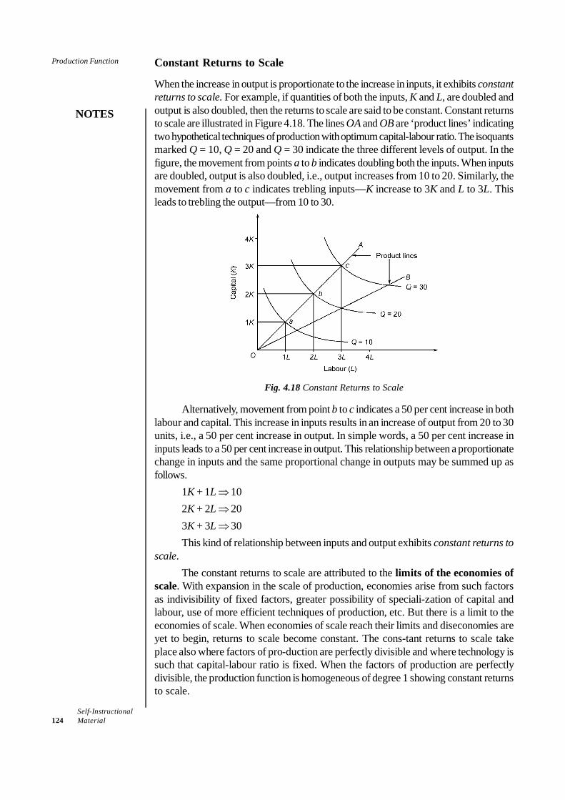
Self-Instructional124 Material
Production Function
NOTES
Constant Returns to Scale
When the increase in output is proportionate to the increase in inputs, it exhibits constantreturns to scale. For example, if quantities of both the inputs, K and L, are doubled andoutput is also doubled, then the returns to scale are said to be constant. Constant returnsto scale are illustrated in Figure 4.18. The lines OA and OB are ‘product lines’ indicatingtwo hypothetical techniques of production with optimum capital-labour ratio. The isoquantsmarked Q = 10, Q = 20 and Q = 30 indicate the three different levels of output. In thefigure, the movement from points a to b indicates doubling both the inputs. When inputsare doubled, output is also doubled, i.e., output increases from 10 to 20. Similarly, themovement from a to c indicates trebling inputs—K increase to 3K and L to 3L. Thisleads to trebling the output—from 10 to 30.
Fig. 4.18 Constant Returns to Scale
Alternatively, movement from point b to c indicates a 50 per cent increase in bothlabour and capital. This increase in inputs results in an increase of output from 20 to 30units, i.e., a 50 per cent increase in output. In simple words, a 50 per cent increase ininputs leads to a 50 per cent increase in output. This relationship between a proportionatechange in inputs and the same proportional change in outputs may be summed up asfollows.
1K + 1L ⇒ 102K + 2L ⇒ 203K + 3L ⇒ 30This kind of relationship between inputs and output exhibits constant returns to
scale.The constant returns to scale are attributed to the limits of the economies of
scale. With expansion in the scale of production, economies arise from such factorsas indivisibility of fixed factors, greater possibility of speciali-zation of capital andlabour, use of more efficient techniques of production, etc. But there is a limit to theeconomies of scale. When economies of scale reach their limits and diseconomies areyet to begin, returns to scale become constant. The cons-tant returns to scale takeplace also where factors of pro-duction are perfectly divisible and where technology issuch that capital-labour ratio is fixed. When the factors of production are perfectlydivisible, the production function is homogeneous of degree 1 showing constant returnsto scale.

Self-InstructionalMaterial 125
Production Function
NOTES
Decreasing Returns to Scale
The firms are faced with decreasing returns to scale when a certain proportionateincrease in inputs, K and L, leads to a less than proportionate increase in output. Forexample, when inputs are doubled and output is less than doubled, then decreasingreturns to scale is in operation. The decreasing returns to scale is illustrated in Figure4.19. As the figure shows, when the inputs K and L are doubled, i.e., when capital-labour combination is increased from 1K + 1L to 2K + 2L, the output increases from10 to 18 units. This means that when capital and labour are increased by 100 per cent,output increases by only 80 per cent. That is, increasing output is less that theproportionate increase in inputs. Similarly, movement from point b to c indicates a 50per cent increase in the inputs. But, the output increases by only 33.3 per cent. Thisexhibits decreasing returns to scale.
Fig. 4.19 Decreasing Return to Scale
Causes of Diminishing Return to Scale
The decreasing returns to scale are attributed to the diseconomies of scale. Theeconomists find that the most important factor causing diminishing returns to scale is‘the diminishing return to management’, i.e., managerial diseconomies. As the size ofthe firms expands, managerial efficiency decreases. Another factor responsible fordiminishing returns to scale is the limitedness or exhaustibility of the natural resources.For example, doubling of coal mining plant may not double the coal output because oflimitedness of coal deposits or difficult accessibility to coal deposits. Similarly, doublingthe fishing fleet may not double the fish output because availability of fish may decreasein the ocean when fishing is carried out on an increased scale.
4.5 SUMMARY
• Production function is a mathematical presentation of input-output relationship.More specifically, a production function states the technological relationshipbetween inputs and output in the form of an equation, a table or a graph.
• Short-run is a period in which supply of capital is inelastic. In the short-run,therefore, the firm can increase coal production by increasing only labour sincethe supply of capital in the short run is fixed.
Check Your Progress
8. State the law ofdiminishing returns.
9. Define an isoquantcurve.
10. Name the otherforms of isoquants.
11. Define elasticity ofsubstitution.
12. What are the threekinds of return toscale?
13. State whichsentence is incorrect
(a) Isoquants have anegative slope
(b) Isoquants areconvex to theorigin
(c) Upper isoquantsrepresent alower level ofoutput
(d) In the isoquantmap, each upperisoquantindicates a largerinput-combinationthan the lowerones, and eachsuccessive upperisoquantindicates a higherlevel of outputthan the lowerones.

Self-Instructional126 Material
Production Function
NOTES
• Long-run is a period in which supply of both labour and capital is elastic. In thelong-run, therefore, the firm can employ more of both capital and labour.
• There are two kinds of production functions:(i) Short-run production function(ii) Long-run production function
• Break-even analysis or what is also known as profit contribution analysis is animportant analytical technique used to study the relationship between the totalcosts, total revenue and total profits and losses over the whole range of stipulatedoutput. The break-even analysis is a technique of having a preview of profitprospects and a tool of profit planning.
• Contribution analysis is the analysis of incremental revenue and incrementalcost of a business decision or business activity.
• Another variation of the break-even chart is called profit-volume analysis chartor graph. In this chart, the horizontal axis represents the sales volume and thevertical axis shows profit or loss. The profit line is graphed by computing theprofit or loss consisting of the difference between sales revenue and the totalcost at each volume.
• The law of diminishing returns states that when more and more units of a variableinput are used with a given quantity of fixed inputs, the total output may initiallyincrease at increasing rate and then at a constant rate, but it will eventuallyincrease at diminishing rates.
• An isoquant curve can be defined as the locus of points representing variouscombinations of two inputs—capital and labour—yielding the same output.
• Isoquants, i.e., production indifference curves, have the same properties asconsumer’s indifference curves.
• Economic region is that area of production plane in which substitution betweentwo inputs is technically feasible without affecting the output. This area is markedby locating the points on the isoquants at which MRTS = 0.
• The other forms of isoquants are— linear isoquants, isoquants with fixed factorproportion or L-shaped isoquants.
• The elasticity of substitution (s) is formally defined as the percentage change inthe capital-labour ratio (K/L) divided by the percentage change in marginal rateof technical substitution (MRTS).
• There are three kinds of returns to scale:(i) Increasing returns to scale(ii) Constant returns to scale(iii) Diminishing returns to scale
• When inputs, K and L, are increased at a certain proportion and output increasesmore than proportionately, it exhibits increasing returns to scale.
• When the increase in output is proportionate to the increase in inputs, it exhibitsconstant returns to scale.
• The firms are faced with decreasing returns to scale when a certain proportionateincrease in inputs, K and L, leads to a less than proportionate increase in output.
Self-InstructionalMaterial 127
Production Function
NOTES
4.6 KEY TERMS
• Production function: It is a mathematical presentation of input-output relationship.• Isoquant curve: An isoquant curve can be defined as the locus of points
representing various combinations of two inputs—capital and labour—yieldingthe same output.
• Elasticity of substitution: The elasticity of substitution (s) is defined as thepercentage change in the capital-labour ratio (K/L) divided by the percentagechange in marginal rate of technical substitution (MRTS).
• Break-even analysis: The break-even analysis is a technique of having a previewof profit prospects and a tool of profit planning.
4.7 ANSWERS TO ‘CHECK YOUR PROGRESS’
1. Production function is a mathematical presentation of input-output relationship.More specifically, a production function states the technological relationshipbetween inputs and output in the form of an equation, a table or a graph.
2. There are two kinds of production functions:• Short-run production function• Long-run production function
3. The break-even analysis is a technique of having a preview of profit prospectsand a tool of profit planning. It integrates the cost and revenue estimates toascertain the profits and losses associated with different levels of output.
4. Contribution analysis is the analysis of incremental revenue and incrementalcost of a business decision or business activity.
5. In profit-volume analysis chart, the horizontal axis represents the sales volumeand the vertical axis shows profit or loss. The profit line is graphed by computingthe profit or loss consisting of the difference between sales revenue and thetotal cost at each volume.
6. (a) Study the relationship between the total costs, total revenue and total profitsand losses over the whole range of stipulated output
7. (c) Break-even analysis cannot serve a useful purpose in production planning ifrelevant data can be easily obtained
8. The law of diminishing returns states that when more and more units of a variableinput are used with a given quantity of fixed inputs, the total output may initiallyincrease at increasing rate and then at a constant rate, but it will eventuallyincrease at diminishing rates.
9. An isoquant curve can be defined as the locus of points representing variouscombinations of two inputs—capital and labour—yielding the same output.
10. The other forms of isoquants are— linear isoquants, isoquants with fixed factorproportion or L-shaped isoquants.
11. The elasticity of substitution (s) is defined as the percentage change in the capital-labour ratio (K/L) divided by the percentage change in marginal rate of technicalsubstitution (MRTS).
Self-Instructional128 Material
Production Function
NOTES
12. There are three kinds of returns to scale:• Increasing returns to scale• Constant returns to scale• Diminishing returns to scale
13. (c) Upper isoquants represent a lower level of output
4.8 QUESTIONS AND EXERCISES
Short-Answer Questions
1. Differentiate between a short run and long run.2. What are the limitations of break-even analysis?3. State the assumptions of law of diminishing returns.4. Write a short note on economic region of production.5. What are the reasons behind diminishing return to scale?
Long-Answer Questions
1. Discuss break-even analysis under both linear and non-linear cost and revenuefunctions. State the uses of break-even analysis.
2. State the law of diminishing returns. Explain the three stages in the applicationof law of diminishing returns with the help of a diagram.
3. List the assumptions of an isoquant curve. Explain the properties of isoquantcurves.
4. Explain the laws of return to scale and the reasons behind their occurrence.
4.9 FURTHER READING/ENDNOTES
Varshney and Maheshwari. 2011. Managerial Economics. New Delhi: Sultan Chandand Sons.
Mankar, V. G. 1982. Business Economics. New Delhi: Himalya Publishing House.Dufty, N.F. 1966. Managerial Economics. New York: Asia Publishing House.
Endnotes
1. Koutsoyiannis, A. op. cit., p. 70.2. Supply of capital may, of course, be elastic in the short-run for an individual firm
under perfect competition but not for all the firms put together. Therefore, for thesake of convenience in explaining the laws of production, we will continue to assumethat, in the short-run, supply of capital remains inelastic.
3. This production function was constructed first by Paul H. Douglas in his book TheTheory of Wages (Macmillan, NY, 1924). The function was developed further byC.W. Cobb and Paul H. Douglas in their joint paper ‘A Theory Production’ in Am.Eco. Rev., March 1928. Since then this production function is known as Cobb-Douglas Production Function.
4. The concept of economic region is discussed in detail in section 4.4.3.
Self-InstructionalMaterial 129
Cost and Revenue
NOTES
UNIT 5 COST AND REVENUE
Structure5.0 Introduction5.1 Unit Objectives5.2 Cost Concepts5.3 Short and Long-Run Cost Curves
5.3.1 Cost Curves and the Law of Diminishing Returns5.4 Total, Marginal and Average Revenues
5.4.1 Price Elasticity of Demand5.4.2 Measuring Price Elasticity from a Demand Function5.4.3 Price Elasticity and Total Revenue5.4.4 Price Elasticity and Marginal Revenue5.4.5 Determinants of Price Elasticity of Demand5.4.6 Cross-Elasticity of Demand5.4.7 Income-Elasticity of Demand5.4.8 Advertisement or Promotional Elasticity of Sales5.4.9 Elasticity of Price Expectations
5.5 Summary5.6 Key Terms5.7 Answers to ‘Check Your Progress’5.8 Questions and Exercises5.9 Further Reading/Endnotes
5.0 INTRODUCTION
Business decisions are generally taken on the basis of money values of the inputs andoutputs. The cost of production is an important factor in almost all business analysis andbusiness decision-making, especially those pertaining to (a) locating the weak points inproduction management (b) minimizing the cost (c) finding the optimum level of output(d) determining price and dealers, margin and (e) estimating or projecting the cost ofbusiness operation. Cost analysis assumes a great significance in all major businessdecisions because the term ‘cost’ has different meanings under different settings and issubject to varying interpretations. It is, therefore, essential that only the relevant conceptof costs is used in the business decisions.
5.1 UNIT OBJECTIVES
After going through this unit, you will be able to:• Understand the cost concepts that are relevant to business operations• Discuss short and long-run cost curves• Explain total, marginal and average revenues and their relationship with elasticity
of demand
5.2 COST CONCEPTS
The cost concepts that are relevant to business operations and decisions can be groupedon the basis of their nature and purpose under two overlapping categories: (i) costconcepts used for accounting purposes, and (ii) analytical cost concepts used in economicanalysis of business activities. We will discuss some important concepts of the two
Self-Instructional130 Material
Cost and Revenue
NOTES
categories. It is important to note here that this classification of cost concepts is only amatter of analytical convenience.
Accounting Cost
1. Opportunity cost and actual cost: The opportunity cost is the opportunity lost. Anopportunity to make income is lost because of scarcity of resources like land, labour,capital. We know that resources available to any person, firm or society are scarce buthave alternative uses with different returns. Income maximizing resource owners puttheir scarce resources to their most productive use and thus, they forego the incomeexpected from the second best use of the resources. Thus, the opportunity cost may bedefined as the expected returns from the second best use of the resources that areforegone due to scarcity of resources. The opportunity cost is also called alternativecost. Had the resource available to a person, a firm or a society been unlimited, therewould be no opportunity cost.
To explain and illustrate the concept of opportunity cost, suppose a firm has a sumof ` 100,000 for which it has only two alternative uses. It can buy either a printingmachine or a photo copier, both having a productive life of 10 years. From the printingmachine, the firm expects an annual income of ̀ 20,000 and from the photo copier, ̀15,000. A profit maximizing firm would invest its money in the printing machine andforego the expected income from the photo copier. The opportunity cost of the incomefrom printing machine is the expected income from the photo copier, i.e., ̀ 15,000. Inassessing the alternative cost, both explicit and implicit costs are taken into account.
Associated with the concept of opportunity cost is the concept of economic rentor economic profit. In our example of expected earnings firm printing machine, theeconomic rent of the printing machine is the excess of its earning over the incomeexpected from the photo copier. That is, economic rent of the printing machine equals ̀20,000 – ̀ 15,000 = ̀ 5,000. The implication of this concept for a businessman is thatinvesting in the printing machine is preferable so long as its economic rent is greater thanzero. Also, if firms know the economic rent of the various alternative uses of theirresources, it will be helpful in choosing of the best investment avenue.2. Business costs and full costs: Business costs include all the expenses that areincurred to carry out a business. The concept of business costs is similar to the actual orreal costs. Business costs “include all the payments and contractual obligations made bythe firm together with the book cost of depreciation on plant and equipment.1” Businesscosts are used for calculating business profits and losses and for filing returns for income-tax and also for other legal purposes.
The concept of full cost, includes business costs, opportunity cost and normalprofit. The opportunity cost includes the foregone expected earning from the secondbest use of the resources, or the market rate of interest on the total money capital andalso the value of an entrepreneur’s own services that are not charged for in the currentbusiness. Normal profit is a necessary minimum earning in addition to the opportunitycost, which a firm must receive to remain in its present occupation.3. Actual or explicit costs and implicit or imputed costs: Actual or explicit costsare those which are actually incurred by the firm in payment for labour, material, plant,building, machinery, equipment, travelling and transport, advertisement. The total moneyexpenses, recorded in the books of accounts are, for all practical purposes, the actualcosts. In our example, the cost of printing machine, i.e., ` 100,000 is the actual cost.Actual cost comes under the accounting cost concept.
Self-InstructionalMaterial 131
Cost and Revenue
NOTES
In contrast to explicit costs, there are certain other costs that do not take the formof cash outlays, nor do they appear in the accounting system. Such costs are known asimplicit or imputed costs. Opportunity cost is an important example of implicit cost. Forexample, suppose an entrepreneur does not utilize his services in his own business andworks as a manager in some other firm on a salary basis. If he sets up his own business,he foregoes his salary as manager. This loss of salary is the opportunity cost of incomefrom his own business. This is an implicit cost of his own business. Thus, implicit wages,rent, and implicit interest are the wages, rent and interest that an owner’s labour, buildingand capital respectively, can earn from their second best use.
Implicit costs are not taken into account while calculating the loss or gains of thebusiness, but they form an important consideration in deciding whether or not to retain afactor in its present use. The explicit and implicit costs together make the economiccost.4. Out-of-pocket and book costs: The items of expenditure that involve cash paymentsor cash transfers, both recurring and non-recurring, are known as out-of-pocket costs.All the explicit costs (e.g., wages, rent, interest, cost of materials and maintenance,transport expenditure, electricity and telephone expenses) fall in this category. On thecontrary, there are certain actual business costs that do not involve cash payments, buta provision is therefore made in the books of account and they are taken into accountwhile finalizing the profit and loss accounts. Such expenses are known as book costs.In a way, these are payments made by a firm to itself. Depreciation allowances andunpaid interest on the owner’s own funds are the example of book costs.
Analytical Cost
1. Fixed and variable costs: Fixed costs are those that are fixed in volume for acertain quantity of output. Fixed cost does not vary with variation in the output betweenzero and a certain level of output. In other words, costs that do not vary or are fixed fora certain level of output are known as fixed costs. The fixed costs include (i) costs ofmanagerial and administrative staff, (ii) depreciation of machinery, building and otherfixed assets, (iii) maintenance of land. The concept of fixed cost is associated with theshort-run.
Variable costs are those which vary with the variation in the total output. Variablecosts include cost of raw material, running cost of fixed capital, such as fuel, repairs,routine maintenance expenditure, direct labour charges associated with the level of output,and the costs of all other inputs that vary with output.2. Total, average and marginal costs: Total cost (TC) is the total actual cost incurredon the production of goods and service. It refers to the total outlays of money expenditure,both explicit and implicit, on the resources used to produce a given level of output. Itincludes both fixed and variable costs. The total cost for a given output is given by thecost function.
Average cost (AC) is of statistical nature—it is not actual cost. It is obtained bydividing the total cost (TC) by the total output (Q), i.e.,
AC = T CQ
Marginal cost (MC) is defined as the addition to the total cost on account ofproducing one additional unit of the product. Or, marginal cost is the cost of the marginal

Self-Instructional132 Material
Cost and Revenue
NOTES
unit produced. Marginal cost is calculated as TCn – TCn–1 where n is the number of unitsproduced. Using cost function, MC can be defined as
MC = TCQ
∂∂
Total, average and marginal cost concepts are used in the economic analysis offirm’s production activities. These cost concepts are discussed in further detail in thefollowing section.3. Short-run and long-run costs: Short-run and long-run cost concepts are related tovariable and fixed costs, respectively, and often figure in economic analysisinterchangeably.
Short-run costs are those that have a short-run implication in the process ofproduction. Such costs are made once e.g., payment of wages, cost of raw materials.Such costs cannot be used again and again. From analytical point of view, short-runcosts are those that vary with the variation in output, the size of the firm remaining thesame. Therefore, short-run costs are treated as variable costs.
Long-run costs, on the other hand, are those that have long-run implications inthe process of production, i.e., they are used over a long range of output. The costs thatare incurred on the fixed factors like plant, building, machinery, etc., are known as long-run costs. It is important to note that the running cost and depreciation of the capitalassets are included in the short-run or variable costs.
Furthermore, long-run costs are by implication the same as fixed costs. In thelong run, however, even the fixed costs become variable costs as the size of the firm orscale of production increases. Broadly speaking, ‘the short-run costs are those associatedwith variables in the utilization of fixed plant or other facilities whereas long-run costsare associated with the changes in the size and kind of plant.’2
4. Incremental costs and sunk costs: Conceptually, incremental costs are closelyrelated to the concept of marginal cost but with a relatively wider connotation. Whilemarginal cost refers to the cost of the marginal unit (generally one unit) of output,incremental cost refers to the total additional cost associated with the decisions to expandthe output or to add a new variety of product. The concept of incremental cost is basedon the fact that in the real world, it is not practicable (for lack of perfect divisibility ofinputs) to employ factors for each unit of output separately. Besides, in the long run,when firms expand their production, they hire more of men, materials, machinery andequipments. The expenditures of this nature are incremental costs — not the marginalcost (as defined earlier). Incremental costs arise also owing to the change in productlines, addition or introduction of a new product, replacement of worn out plant andmachinery, replacement of old technique of production with a new one.
The sunk costs are those which are made once and for all and cannot be altered,increased or decreased, by varying the rate of output, nor can they be recovered. Forexample, once it is decided to make incremental investment expenditure and the fundsare allocated and spent, all the preceding costs are considered to be the sunk costs. Thereason is, such costs are based on the prior commitment and cannot be revised orreversed or recovered when there is a change in market conditions or change in businessdecisions.5. Historical and replacement costs: Historical cost refers to the cost incurred inpast on the acquisition of productive assets, e.g. land, building, machinery whereas
Check Your Progress
1. Define opportunitycost.
2. What is meant bybusiness costs?
3. What is full cost?4. What are sunk costs?5. Define historical
costs.
Self-InstructionalMaterial 133
Cost and Revenue
NOTES
replacement cost refers to the outlay that has to be made for replacing an old asset.These concepts owe their significance to the unstable nature of price behaviour. Stableprices over time, other things given, keep historical and replacement costs on par witheach other. Instability in asset prices makes the two costs differ from each other.
Historical cost of assets is used for accounting purposes, in the assessment ofthe net worth of the firm. The replacement cost figures in business decisions regardingthe renovation of the firm.6. Private and social costs: We have so far discussed the cost concepts that arerelated to the working of the firm and that are used in the cost-benefit analysis ofbusiness decisions. Such costs fall in the category of private costs. There are, however,certain other costs that arise due to the functioning of the firm but do not normally figurein the business decisions nor are such costs explicitly borne by the firms. The costs inthis category are borne by the society. Thus, the total cost generated by a firm’s workingmay be divided into two categories: (i) those paid out or provided for by the firms, and(ii) those not paid or borne by the firms including the use of resources freely availableplus the disutility created in the process of production. The costs of the former categoryare known as private costs and of the latter category are known as external or socialcosts. To mention a few examples of social cost, Mathura Oil Refinery discharging itswastage in the Yamuna river causes water pollution. Mills and factories located in a citycause air pollution, environment pollution and so on. Such costs are termed as externalcosts from the firm’s point of view and social costs from the society’s point of view.
The relevance of the social costs lies in the social cost-benefit analysis of theoverall impact of a firm’s operation on the society as a whole and in working out thesocial cost of private gains. A further distinction between private cost and social cost is,therefore, in order.
Private costs are those which are actually incurred or provided for by an individualor a firm on the purchase of goods and services from the market. For a firm, all theactual costs, both explicit and implicit, are private costs. Private costs are internalizedcosts that are incorporated in the firm’s total cost of production.
Social costs on the other hand, refer to the total cost borne by the society due toproduction of a commodity. Social costs includes both private cost and the external cost.Social cost includes (a) the cost of resources for which the firm is not required to pay aprice, i.e., atmosphere, rivers, lakes and also for the use of public utility services3 likeroadways, drainage system, and (b) the cost in the form of ‘disutility’ created throughair, water, noise and environment pollution. The costs of category (b) are generallyassumed to equal the total private and public expenditure incurred to safeguard theindividual and public interest against the various kinds of health hazards and social tensioncreated by the production system. The private and public expenditure, however, serveonly as an indicator of ‘public disutility’—they do not give the exact measure of thepublic disutility or the social costs.
5.3 SHORT AND LONG-RUN COST CURVES
The cost-output relations are determined by the cost function and are exhibited throughcost curves. The shape of the cost curves depends on the nature of the cost function.Cost functions are derived from actual cost data of the firms. Given the cost data, cost
Check Your Progress
6. Fixed costs are:(a) Expenses
incurred to carryout a business
(b) Cost fixed involume for acertain quantityof output
(c) Those which areactually incurredby the firm inpayment forlabour, material,plant, building,machinery,equipment,travelling andtransport,advertisement
(d) Closely related tothe concept ofmarginal cost butwith a relativelywiderconnotation
7. State which of themis true(a) Sunk cost and
incrementalcosts are same
(b) Historical costrefers to the costincurred inreplacing oldassets
(c) Incrementalcosts are closelyrelated to theconcept ofmarginal cost butwith a relativelywiderconnotation
(d) Private costsrefer to the totalcost borne bythe society dueto production ofa commodity.
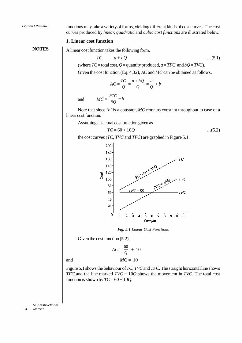
Self-Instructional134 Material
Cost and Revenue
NOTES
functions may take a variety of forms, yielding different kinds of cost curves. The costcurves produced by linear, quadratic and cubic cost functions are illustrated below.
1. Linear cost function
A linear cost function takes the following form. TC = a + bQ …(5.1)
(where TC = total cost, Q = quantity produced, a = TFC, and bQ = TVC).Given the cost function (Eq. 4.32), AC and MC can be obtained as follows.
AC =TCQ =
a bQQ+
=aQ + b
and MC = TC bQ
∂=
∂
Note that since ‘b’ is a constant, MC remains constant throughout in case of alinear cost function.
Assuming an actual cost function given asTC = 60 + 10Q …(5.2)
the cost curves (TC, TVC and TFC) are graphed in Figure 5.1.
Fig. 5.1 Linear Cost Functions
Given the cost function (5.2),
AC =60Q
+ 10
and MC = 10
Figure 5.1 shows the behaviour of TC, TVC and TFC. The straight horizontal line showsTFC and the line marked TVC = 10Q shows the movement in TVC. The total costfunction is shown by TC = 60 + 10Q.

Self-InstructionalMaterial 135
Cost and Revenue
NOTES
Fig. 5.2 AC and MC Curves Derived from Linear Cost Function
More important is to notice the behaviour of AC and MC curves in Figure 5.2.Note that, in case of a linear cost function, MC = AVC and it remains constant, while ACcontinues to decline with the increase in output. This is so simply because of the logic ofthe linear cost function.2. Quadratic cost functionA quadratic cost function is of the form
TC = a + bQ + Q2 ....(5.3)where a and b are constants and TC and Q are total cost and total output,
respectively.Given the cost function (5.3), AC and MC can be obtained as follows.
AC =TCQ =
2a bQ QQ
+ +...(5.4)
=aQ + b + Q
MC =TCQ
∂∂
= b + 2Q ...(5.5)
Let the actual (or estimated) cost function be given asTC = 50 + 5Q + Q2 …(5.6)
Given the cost function (5.6),
AC =50Q Q + 5
and MC =CQ∂∂
= 5 + 2Q
The cost curves that emerge from the cost function (5.6) are graphed in Figure5.3 (a) and (b). As shown in panel (a), while fixed cost remains constant at 50, TVC isincreasing at an increasing rate. The rising TVC sets the trend in the total cost (TC).Panel (b) shows the behaviour of AC, MC and AVC in a quadratic cost function. Notethat MC and AVC are rising at a constant rate whereas AC first declines and thenincreases.
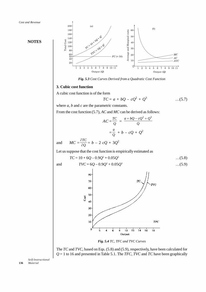
Self-Instructional136 Material
Cost and Revenue
NOTES
Output ( )Q Output ( )Q
Tota
l Cos
t
Ave
rage
and
Mar
gina
l cos
ts
1 1
20
20
30
1040
40
60
60
50
50
80100120140160180200
2 23 34 45 56 67 78 89 910 1011 11
( )a( )b
FC (= 50)MCACAVC
TC
Q Q
= 50 + 5+
2
TVC Q Q
= 5+
2
0
Fig. 5.3 Cost Curves Derived from a Quadratic Cost Function
3. Cubic cost functionA cubic cost function is of the form
TC = a + bQ – cQ2 + Q3 …(5.7)where a, b and c are the parametric constants.From the cost function (5.7), AC and MC can be derived as follows:
AC =TCQ =
2 3a bQ cQ QQ
+ − +
=aQ + b – cQ + Q2
and MC =TCQ
∂∂
= b – 2 cQ + 3Q2
Let us suppose that the cost function is empirically estimated as TC = 10 + 6Q – 0.9Q2 + 0.05Q3 …(5.8)and TVC = 6Q – 0.9Q2 + 0.05Q3 …(5.9)
Fig. 5.4 TC, TFC and TVC Curves
The TC and TVC, based on Eqs. (5.8) and (5.9), respectively, have been calculated forQ = 1 to 16 and presented in Table 5.1. The TFC, TVC and TC have been graphically
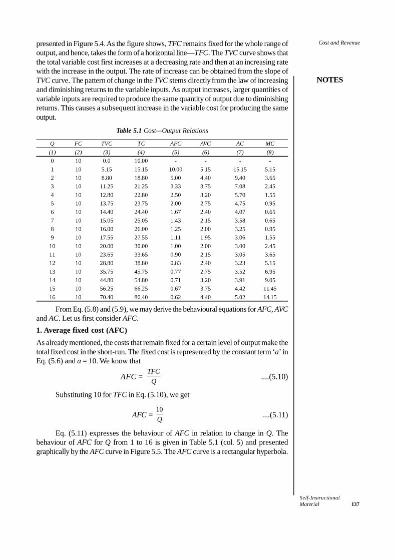
Self-InstructionalMaterial 137
Cost and Revenue
NOTES
presented in Figure 5.4. As the figure shows, TFC remains fixed for the whole range ofoutput, and hence, takes the form of a horizontal line—TFC. The TVC curve shows thatthe total variable cost first increases at a decreasing rate and then at an increasing ratewith the increase in the output. The rate of increase can be obtained from the slope ofTVC curve. The pattern of change in the TVC stems directly from the law of increasingand diminishing returns to the variable inputs. As output increases, larger quantities ofvariable inputs are required to produce the same quantity of output due to diminishingreturns. This causes a subsequent increase in the variable cost for producing the sameoutput.
Table 5.1 Cost—Output Relations
Q FC TVC TC AFC AVC AC MC(1) (2) (3) (4) (5) (6) (7) (8)0 10 0.0 10.00 - - - -1 10 5.15 15.15 10.00 5.15 15.15 5.152 10 8.80 18.80 5.00 4.40 9.40 3.653 10 11.25 21.25 3.33 3.75 7.08 2.454 10 12.80 22.80 2.50 3.20 5.70 1.555 10 13.75 23.75 2.00 2.75 4.75 0.956 10 14.40 24.40 1.67 2.40 4.07 0.657 10 15.05 25.05 1.43 2.15 3.58 0.658 10 16.00 26.00 1.25 2.00 3.25 0.959 10 17.55 27.55 1.11 1.95 3.06 1.55
10 10 20.00 30.00 1.00 2.00 3.00 2.4511 10 23.65 33.65 0.90 2.15 3.05 3.6512 10 28.80 38.80 0.83 2.40 3.23 5.1513 10 35.75 45.75 0.77 2.75 3.52 6.9514 10 44.80 54.80 0.71 3.20 3.91 9.0515 10 56.25 66.25 0.67 3.75 4.42 11.4516 10 70.40 80.40 0.62 4.40 5.02 14.15
From Eq. (5.8) and (5.9), we may derive the behavioural equations for AFC, AVCand AC. Let us first consider AFC.1. Average fixed cost (AFC)As already mentioned, the costs that remain fixed for a certain level of output make thetotal fixed cost in the short-run. The fixed cost is represented by the constant term ‘a’ inEq. (5.6) and a = 10. We know that
AFC = TFC
Q ....(5.10)
Substituting 10 for TFC in Eq. (5.10), we get
AFC = 10Q ....(5.11)
Eq. (5.11) expresses the behaviour of AFC in relation to change in Q. Thebehaviour of AFC for Q from 1 to 16 is given in Table 5.1 (col. 5) and presentedgraphically by the AFC curve in Figure 5.5. The AFC curve is a rectangular hyperbola.

Self-Instructional138 Material
Cost and Revenue
NOTES
2. Average variable cost (AVC)
As defined above, AVC = TVC
Q
Given the TVC function (Eq. 5.9), we may express AVC as follows:
AVC =2 36 0.9 0.05Q Q Q
Q− +
= 6 – 0.9Q + 0.05Q2 ...(5.12)
Having derived the AVC function in Eq. (5.12), we can easily obtain the behaviourof AVC in response to change in Q. The behaviour of AVC for Q = 1 to 16 is given inTable 5.1 (col. 6).
Fig. 5.5 Short-run Curves
Critical value of AVC: From Eq. (5.6), we may compute the critical value of Qin respect of AVC. The critical value of Q (in respect of AVC) is one that minimizesAVC. The AVC will be minimum when its (decreasing) rate of change equals zero. Thiscan be accomplished by differentiating Eq. (5.11) and setting it equal to zero. Thus,critical value of Q can be obtained as
Critical value of Q =AVC
Q∂∂
= – 0.9 + 0.10 Q = 0
0.10 Q = 0.9Q = 9
In our example, the critical value of Q = 9. This can be verified from Table 5.1.The AVC is minimum (1.95) at output 9.
3. Average cost (AC)
The average cost (AC) is defined as AC = TCQ .
Substituting cost function given in Eq. (5.8) for TC in the above equation, we get

Self-InstructionalMaterial 139
Cost and Revenue
NOTES
AC = 2 310 6 0.9 0.05Q Q Q
Q+ − +
=10Q + 6 – 0.9Q + 0.05Q2 ...(5.13)
The Eq. (5.13) gives the behaviour of AC in response to change in Q. The behaviourof AC for Q = 1 to 16 is given in Table 5.1 and graphically presented in Figure 5.5 by theAC curve. Note that AC curve is U-shaped.
Minimization of AC: One objective of business firms is to minimize AC of theirproduct or, which is the same as, to optimize the output. The level of output that minimizesAC can be obtained by differentiating Eq. 5.10 and setting it equal to zero. Thus, theoptimum value of Q can be obtained as follows.
210 0.9 0.1AC Q
Q Q∂
= − +∂
= 0
When simplified this equation takes the form of a quadratic equation as– 10 – 0.9Q2 + 0.1Q3 = 0
or Q3 – 9Q2 – 100 = 0 ...(5.14)
By solving Eq. (5.14) we get Q = 10.Thus, the critical value of output in respect of AC is 10. That is AC reaches its
minimum at Q = 10. This can be verified from Table 5.1.Marginal cost (MC): The concept of marginal cost (MC) is particularly useful
in economic analysis. MC is technically the first derivative of the TC function. Given theTC function in Eq. (5.8), the MC function can be obtained as
MC =TCQ
∂∂ = 6 – 1.8Q + 0.15Q2 ...(5.15)
Equation (5.15) represents the behaviour of MC. The behaviour of MC for Q = 1to 16 computed as MC = TCn– TCn–1 is given in Table 5.1 (col. 8) and graphicallypresented by the MC curve in Figure 5.5. The critical value of Q with respect to MC is6 or 7. This can be seen from Table 5.1.
5.3.1 Cost Curves and the Law of Diminishing Returns
We now return to the law of variable proportions and explain it through the cost curves.Figures 5.6 and 5.7 present the short-term law of production, i.e., the law of diminishingreturns. Let us recall the law: it states that when more and more units of a variable inputare applied, other inputs held constant, the returns from the marginal units of the variableinput may initially increase but it decreases eventually. The same law can also beinterpreted in terms of decreasing and increasing costs. The law can then be stated as,if more and more units of a variable input are applied to a given amount of a fixed input,the marginal cost initially decreases, but eventually increases. Both interpretations of thelaw yield the same information—one in terms of marginal productivity of the variableinput, and the other in terms of the marginal cost. The former is expressed through aproduction function and the latter through a cost function.
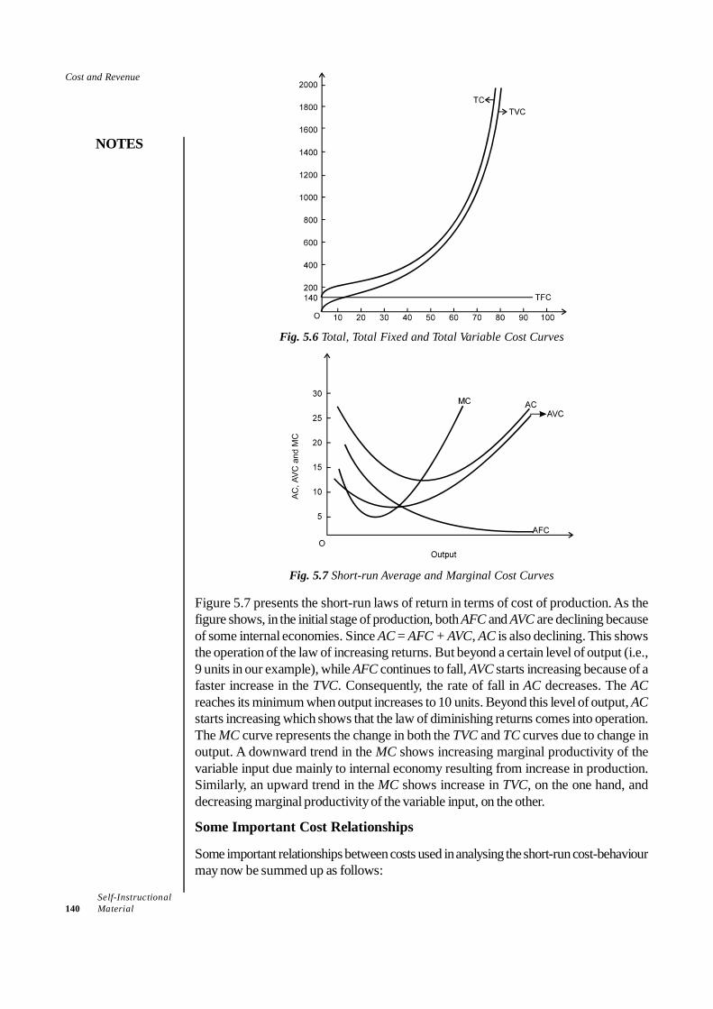
Self-Instructional140 Material
Cost and Revenue
NOTES
Fig. 5.6 Total, Total Fixed and Total Variable Cost Curves
Fig. 5.7 Short-run Average and Marginal Cost Curves
Figure 5.7 presents the short-run laws of return in terms of cost of production. As thefigure shows, in the initial stage of production, both AFC and AVC are declining becauseof some internal economies. Since AC = AFC + AVC, AC is also declining. This showsthe operation of the law of increasing returns. But beyond a certain level of output (i.e.,9 units in our example), while AFC continues to fall, AVC starts increasing because of afaster increase in the TVC. Consequently, the rate of fall in AC decreases. The ACreaches its minimum when output increases to 10 units. Beyond this level of output, ACstarts increasing which shows that the law of diminishing returns comes into operation.The MC curve represents the change in both the TVC and TC curves due to change inoutput. A downward trend in the MC shows increasing marginal productivity of thevariable input due mainly to internal economy resulting from increase in production.Similarly, an upward trend in the MC shows increase in TVC, on the one hand, anddecreasing marginal productivity of the variable input, on the other.
Some Important Cost Relationships
Some important relationships between costs used in analysing the short-run cost-behaviourmay now be summed up as follows:
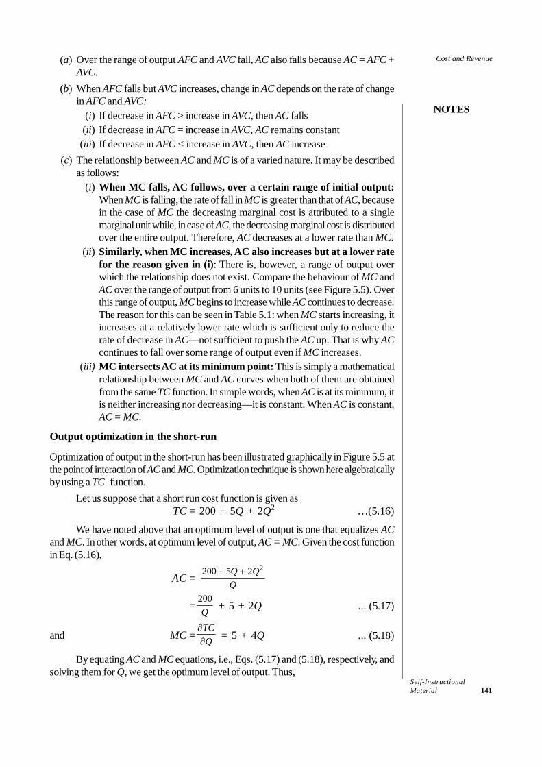
Self-InstructionalMaterial 141
Cost and Revenue
NOTES
(a) Over the range of output AFC and AVC fall, AC also falls because AC = AFC +AVC.
(b) When AFC falls but AVC increases, change in AC depends on the rate of changein AFC and AVC:
(i) If decrease in AFC > increase in AVC, then AC falls(ii) If decrease in AFC = increase in AVC, AC remains constant
(iii) If decrease in AFC < increase in AVC, then AC increase(c) The relationship between AC and MC is of a varied nature. It may be described
as follows:(i) When MC falls, AC follows, over a certain range of initial output:
When MC is falling, the rate of fall in MC is greater than that of AC, becausein the case of MC the decreasing marginal cost is attributed to a singlemarginal unit while, in case of AC, the decreasing marginal cost is distributedover the entire output. Therefore, AC decreases at a lower rate than MC.
(ii) Similarly, when MC increases, AC also increases but at a lower ratefor the reason given in (i): There is, however, a range of output overwhich the relationship does not exist. Compare the behaviour of MC andAC over the range of output from 6 units to 10 units (see Figure 5.5). Overthis range of output, MC begins to increase while AC continues to decrease.The reason for this can be seen in Table 5.1: when MC starts increasing, itincreases at a relatively lower rate which is sufficient only to reduce therate of decrease in AC—not sufficient to push the AC up. That is why ACcontinues to fall over some range of output even if MC increases.
(iii) MC intersects AC at its minimum point: This is simply a mathematicalrelationship between MC and AC curves when both of them are obtainedfrom the same TC function. In simple words, when AC is at its minimum, itis neither increasing nor decreasing—it is constant. When AC is constant,AC = MC.
Output optimization in the short-run
Optimization of output in the short-run has been illustrated graphically in Figure 5.5 atthe point of interaction of AC and MC. Optimization technique is shown here algebraicallyby using a TC–function.
Let us suppose that a short run cost function is given asTC = 200 + 5Q + 2Q2 …(5.16)
We have noted above that an optimum level of output is one that equalizes ACand MC. In other words, at optimum level of output, AC = MC. Given the cost functionin Eq. (5.16),
AC = 2200 5 2Q Q
Q+ +
=200Q + 5 + 2Q ... (5.17)
and MC =TCQ
∂∂ = 5 + 4Q ... (5.18)
By equating AC and MC equations, i.e., Eqs. (5.17) and (5.18), respectively, andsolving them for Q, we get the optimum level of output. Thus,

Self-Instructional142 Material
Cost and Revenue
NOTES
200Q
+ 5 + 2Q = 5 + 4Q
200Q
= 2Q
2Q2 = 200Q = 10
Thus, given the cost function (5.16), the optimum output is 10.
Long-run cost–output relations
By definition, long-run is a period in which all the inputs become variable. The variabilityof inputs is based on the assumption that in the long-run supply of all the inputs, includingthose held constant in the short-run, becomes elastic. The firms are, therefore, in aposition to expand the scale of their production by hiring a larger quantity of all theinputs. The long-run-cost-output relations, therefore, imply the relationship between thechanging scale of the firm and the total output, whereas in the short-run this relationshipis essentially one between the total output and the variable cost (labour).
To understand the long-run-cost-output relations and to derive long-run cost curvesit will be helpful to imagine that a long-run is composed of a series of short-run productiondecisions. As a corollary of this, long-run cost curve is composed of a series of short-runcost curves. We may now derive the long-run cost curves and study their relationshipwith output.Long-run total cost curve (LTC)In order to draw the long-run total cost curve, let us begin with a short-run situation.Suppose that a firm having only one plant has its short-run total cost curve as given bySTC1, in panel (a) of Figure 5.8. Let us now suppose that the firm decides to add twomore plants to its size over time, one after the other. As a result, two more short-run totalcost curves are added to STC1, in the manner shown by STC2 and STC3 in Figure 5.8(a).The LTC can now be drawn through the minimum points of STC1, STC2 and STC3 asshown by the LTC curve corresponding to each STC.
Fig. 5.8 Long-run Total and Average Cost Curves
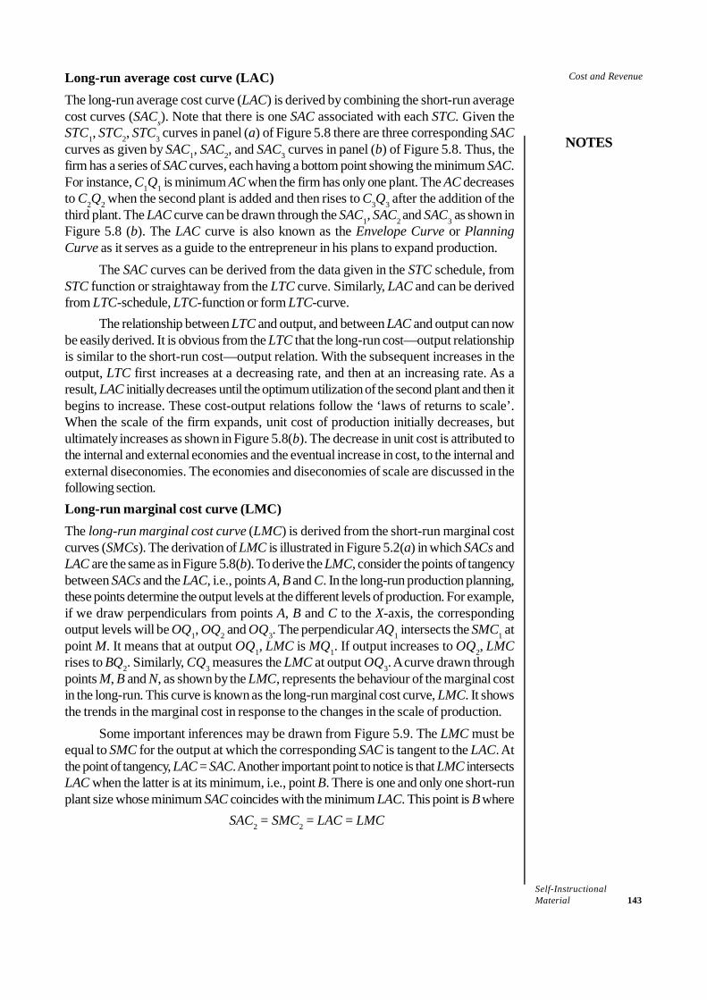
Self-InstructionalMaterial 143
Cost and Revenue
NOTES
Long-run average cost curve (LAC)The long-run average cost curve (LAC) is derived by combining the short-run averagecost curves (SACs). Note that there is one SAC associated with each STC. Given theSTC1, STC2, STC3 curves in panel (a) of Figure 5.8 there are three corresponding SACcurves as given by SAC1, SAC2, and SAC3 curves in panel (b) of Figure 5.8. Thus, thefirm has a series of SAC curves, each having a bottom point showing the minimum SAC.For instance, C1Q1 is minimum AC when the firm has only one plant. The AC decreasesto C2Q2 when the second plant is added and then rises to C3Q3 after the addition of thethird plant. The LAC curve can be drawn through the SAC1, SAC2 and SAC3 as shown inFigure 5.8 (b). The LAC curve is also known as the Envelope Curve or PlanningCurve as it serves as a guide to the entrepreneur in his plans to expand production.
The SAC curves can be derived from the data given in the STC schedule, fromSTC function or straightaway from the LTC curve. Similarly, LAC and can be derivedfrom LTC-schedule, LTC-function or form LTC-curve.
The relationship between LTC and output, and between LAC and output can nowbe easily derived. It is obvious from the LTC that the long-run cost—output relationshipis similar to the short-run cost—output relation. With the subsequent increases in theoutput, LTC first increases at a decreasing rate, and then at an increasing rate. As aresult, LAC initially decreases until the optimum utilization of the second plant and then itbegins to increase. These cost-output relations follow the ‘laws of returns to scale’.When the scale of the firm expands, unit cost of production initially decreases, butultimately increases as shown in Figure 5.8(b). The decrease in unit cost is attributed tothe internal and external economies and the eventual increase in cost, to the internal andexternal diseconomies. The economies and diseconomies of scale are discussed in thefollowing section.Long-run marginal cost curve (LMC)The long-run marginal cost curve (LMC) is derived from the short-run marginal costcurves (SMCs). The derivation of LMC is illustrated in Figure 5.2(a) in which SACs andLAC are the same as in Figure 5.8(b). To derive the LMC, consider the points of tangencybetween SACs and the LAC, i.e., points A, B and C. In the long-run production planning,these points determine the output levels at the different levels of production. For example,if we draw perpendiculars from points A, B and C to the X-axis, the correspondingoutput levels will be OQ1, OQ2 and OQ3. The perpendicular AQ1 intersects the SMC1 atpoint M. It means that at output OQ1, LMC is MQ1. If output increases to OQ2, LMCrises to BQ2. Similarly, CQ3 measures the LMC at output OQ3. A curve drawn throughpoints M, B and N, as shown by the LMC, represents the behaviour of the marginal costin the long-run. This curve is known as the long-run marginal cost curve, LMC. It showsthe trends in the marginal cost in response to the changes in the scale of production.
Some important inferences may be drawn from Figure 5.9. The LMC must beequal to SMC for the output at which the corresponding SAC is tangent to the LAC. Atthe point of tangency, LAC = SAC. Another important point to notice is that LMC intersectsLAC when the latter is at its minimum, i.e., point B. There is one and only one short-runplant size whose minimum SAC coincides with the minimum LAC. This point is B where
SAC2 = SMC2 = LAC = LMC
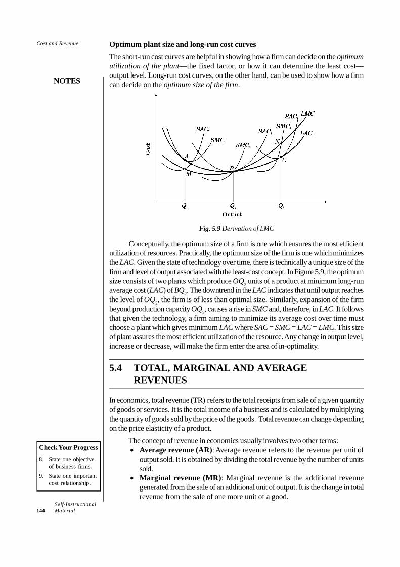
Self-Instructional144 Material
Cost and Revenue
NOTES
Optimum plant size and long-run cost curvesThe short-run cost curves are helpful in showing how a firm can decide on the optimumutilization of the plant—the fixed factor, or how it can determine the least cost—output level. Long-run cost curves, on the other hand, can be used to show how a firmcan decide on the optimum size of the firm.
Fig. 5.9 Derivation of LMC
Conceptually, the optimum size of a firm is one which ensures the most efficientutilization of resources. Practically, the optimum size of the firm is one which minimizesthe LAC. Given the state of technology over time, there is technically a unique size of thefirm and level of output associated with the least-cost concept. In Figure 5.9, the optimumsize consists of two plants which produce OQ2 units of a product at minimum long-runaverage cost (LAC) of BQ2. The downtrend in the LAC indicates that until output reachesthe level of OQ2, the firm is of less than optimal size. Similarly, expansion of the firmbeyond production capacity OQ2, causes a rise in SMC and, therefore, in LAC. It followsthat given the technology, a firm aiming to minimize its average cost over time mustchoose a plant which gives minimum LAC where SAC = SMC = LAC = LMC. This sizeof plant assures the most efficient utilization of the resource. Any change in output level,increase or decrease, will make the firm enter the area of in-optimality.
5.4 TOTAL, MARGINAL AND AVERAGEREVENUES
In economics, total revenue (TR) refers to the total receipts from sale of a given quantityof goods or services. It is the total income of a business and is calculated by multiplyingthe quantity of goods sold by the price of the goods. Total revenue can change dependingon the price elasticity of a product.
The concept of revenue in economics usually involves two other terms:• Average revenue (AR): Average revenue refers to the revenue per unit of
output sold. It is obtained by dividing the total revenue by the number of unitssold.
• Marginal revenue (MR): Marginal revenue is the additional revenuegenerated from the sale of an additional unit of output. It is the change in totalrevenue from the sale of one more unit of a good.
Check Your Progress
8. State one objectiveof business firms.
9. State one importantcost relationship.
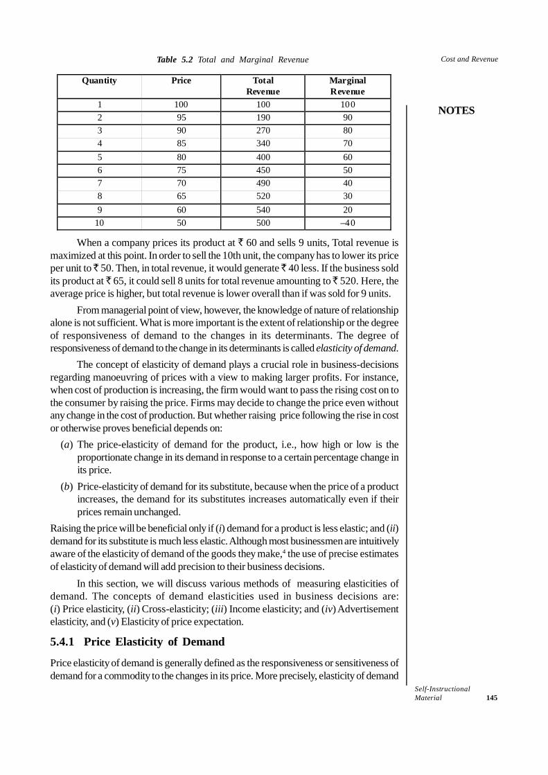
Self-InstructionalMaterial 145
Cost and Revenue
NOTES
Table 5.2 Total and Marginal Revenue
Quantity Price Total Revenue
Marginal Revenue
1 100 100 100 2 95 190 90 3 90 270 80 4 85 340 70 5 80 400 60 6 75 450 50 7 70 490 40 8 65 520 30 9 60 540 20
10 50 500 –40
When a company prices its product at ` 60 and sells 9 units, Total revenue ismaximized at this point. In order to sell the 10th unit, the company has to lower its priceper unit to ̀ 50. Then, in total revenue, it would generate ̀ 40 less. If the business soldits product at ̀ 65, it could sell 8 units for total revenue amounting to ̀ 520. Here, theaverage price is higher, but total revenue is lower overall than if was sold for 9 units.
From managerial point of view, however, the knowledge of nature of relationshipalone is not sufficient. What is more important is the extent of relationship or the degreeof responsiveness of demand to the changes in its determinants. The degree ofresponsiveness of demand to the change in its determinants is called elasticity of demand.
The concept of elasticity of demand plays a crucial role in business-decisionsregarding manoeuvring of prices with a view to making larger profits. For instance,when cost of production is increasing, the firm would want to pass the rising cost on tothe consumer by raising the price. Firms may decide to change the price even withoutany change in the cost of production. But whether raising price following the rise in costor otherwise proves beneficial depends on:
(a) The price-elasticity of demand for the product, i.e., how high or low is theproportionate change in its demand in response to a certain percentage change inits price.
(b) Price-elasticity of demand for its substitute, because when the price of a productincreases, the demand for its substitutes increases automatically even if theirprices remain unchanged.
Raising the price will be beneficial only if (i) demand for a product is less elastic; and (ii)demand for its substitute is much less elastic. Although most businessmen are intuitivelyaware of the elasticity of demand of the goods they make,4 the use of precise estimatesof elasticity of demand will add precision to their business decisions.
In this section, we will discuss various methods of measuring elasticities ofdemand. The concepts of demand elasticities used in business decisions are:(i) Price elasticity, (ii) Cross-elasticity; (iii) Income elasticity; and (iv) Advertisementelasticity, and (v) Elasticity of price expectation.
5.4.1 Price Elasticity of Demand
Price elasticity of demand is generally defined as the responsiveness or sensitiveness ofdemand for a commodity to the changes in its price. More precisely, elasticity of demand

Self-Instructional146 Material
Cost and Revenue
NOTES
is the percentage change in demand as a result of one per cent change in the price of thecommodity. A formal definition of price elasticity of demand (ep) is given as
ep = Percentage change in quantity demanded
Percentage change in price
A general formula5 for calculating coefficient of price elasticity, derived from thisdefinition of elasticity, is given as follows:
ep = Q P Q P
Q P Q PΔ Δ Δ
÷ = ×Δ
= Q PP Q
Δ×
Δ…(5.19)
where Q = original quantity demanded, P = original price, ΔQ = change in quantitydemanded and ΔP = change in price.
It is important to note here that a minus sign (–) is generally inserted in the formulabefore the fraction in order to make the elasticity coefficient a non-negative value.6
The elasticity can be measured between any two points on a demand curve (calledarc elasticity) or at a point (called point elasticity).
The measure of elasticity of demand between any two finite points on a demandcurve is known as arc elasticity. For example, measure of elasticity between points Jand K (Figure 5.10) is the measure of arc elasticity. The movement from point J to Kon the demand curve (Δx) shows a fall in the price from ` 20 to ` 10 so that ΔP = 20– 10 = 10. The fall in price causes an increase in demand from 43 units to 75 units sothat ΔQ = 43 – 75 = – 32. The elasticity between points J and K (moving from J to K)can be calculated by substituting these values into the elasticity formula as follows:
ep = – Q PP Q
Δ⋅
Δ (with minus sign)
= 32 20 1.4910 43−
− ⋅ = ...(5.20)
This means that a one per cent decrease in price of commodity X results in a 1.49per cent increase in demand for it.
Problem in using Arc elasticity: The arc elasticity should be measured and usedcarefully, otherwise it may lead to wrong decisions. Arc elasticity co-efficients differbetween the same two finite points on a demand curve if direction of change in price isreversed. For instance, as estimated in Eq. (5.20), the elasticity between points J andK—moving from J to K equals 1.49. It may be wrongly interpreted that the elasticity ofdemand for commodity X between points J and K equals 1.49 irrespective of the directionof price change. But it is not true. A reverse movement in the price, i.e., the movementfrom point K to J implies a different elasticity co-efficient (0.43). Movement from pointK to J gives P = 10, ΔP = 10 – 20 = –10, Q = 75 and ΔQ = 75 – 43 = 32. By substitutingthese values into the elasticity formula, we get
ep = – 32 10.10 75−
= 0.43 ...(5.21)
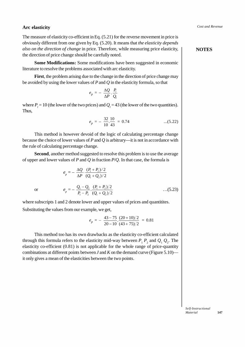
Self-InstructionalMaterial 147
Cost and Revenue
NOTES
Arc elasticity
The measure of elasticity co-efficient in Eq. (5.21) for the reverse movement in price isobviously different from one given by Eq. (5.20). It means that the elasticity dependsalso on the direction of change in price. Therefore, while measuring price elasticity,the direction of price change should be carefully noted.
Some Modifications: Some modifications have been suggested in economicliterature to resolve the problems associated with arc elasticity.
First, the problem arising due to the change in the direction of price change maybe avoided by using the lower values of P and Q in the elasticity formula, so that
ep = – . l
l
PQP Q
ΔΔ
where Pl = 10 (the lower of the two prices) and Ql = 43 (the lower of the two quantities).Thus,
ep = – 32 10.10 43
= 0.74 ...(5.22)
This method is however devoid of the logic of calculating percentage changebecause the choice of lower values of P and Q is arbitrary—it is not in accordance withthe rule of calculating percentage change.
Second, another method suggested to resolve this problem is to use the averageof upper and lower values of P and Q in fraction P/Q. In that case, the formula is
ep = – 1 2
1 2
( ) / 2( ) / 2
P PQP Q Q
+Δ⋅
Δ +
or ep = – 1 2 1 2
1 2 1 2
( ) 2.( ) 2
Q Q P PP P Q Q− +− +
…(5.23)
where subscripts 1 and 2 denote lower and upper values of prices and quantitites.Substituting the values from our example, we get,
ep = – 43 75 (20 10) 2.20 10 (43 75) 2
− +− +
= 0.81
This method too has its own drawbacks as the elasticity co-efficient calculatedthrough this formula refers to the elasticity mid-way between P1 P2 and Q1 Q2. Theelasticity co-efficient (0.81) is not applicable for the whole range of price-quantitycombinations at different points between J and K on the demand curve (Figure 5.10)—it only gives a mean of the elasticities between the two points.
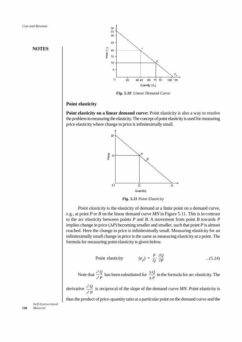
Self-Instructional148 Material
Cost and Revenue
NOTES
Fig. 5.10 Linear Demand Curve
Point elasticity
Point elasticity on a linear demand curve: Point elasticity is also a way to resolvethe problem in measuring the elasticity. The concept of point elasticity is used for measuringprice elasticity where change in price is infinitesimally small.
Fig. 5.11 Point Elasticity
Point elasticity is the elasticity of demand at a finite point on a demand curve,e.g., at point P or B on the linear demand curve MN in Figure 5.11. This is in contrastto the arc elasticity between points P and B. A movement from point B towards Pimplies change in price (ΔP) becoming smaller and smaller, such that point P is almostreached. Here the change in price is infinitesimally small. Measuring elasticity for aninfinitesimally small change in price is the same as measuring elasticity at a point. Theformula for measuring point elasticity is given below.
Point elasticity (ep) = PQ
QP
∂∂⋅ ...(5.24)
Note that QP
∂∂
has been substituted for QP
ΔΔ
in the formula for arc elasticity. The
derivative QP
∂∂
is reciprocal of the slope of the demand curve MN. Point elasticity is
thus the product of price-quantity ratio at a particular point on the demand curve and the

Self-InstructionalMaterial 149
Cost and Revenue
NOTES
reciprocal of the slope of the demand line. The reciprocal of the slope of the straight lineMN at point P is geometrically given by QN/PQ. Therefore,
QP
ΔΔ
= QNPQ
Note that at point P, price P = PQ and Q = OQ. By substituting these values in Eq.(5.24), we get
ep = PQ QN QNOQ PQ OQ
⋅ =
Given the numerical values for QN and OQ, elasticity at point P can be easilyobtained. We may compare here the arc elasticity between points J and K and pointelasticity at point J in Figure 5.10. At point J,
ep = QNOQ
= 108 43
43−
= 1.51
Note that ep = 1.51 is different from various measures of arc elasticities (i.e., ep= 1.49, ep = 0.43, ep = 0.7, and ep = 0.81).
As we will see below, geometrically, QN/OQ = PN/PM. Therefore, elasticity ofdemand at point P (Figure 5.11) may be expressed as
ep = PNPM
Proof: The fact that ep = PN/PM can be proved as follows. Note that inFigure 5.11, there are three triangles—ΔMON, ΔMRP and ΔPQN—and ΔMON, ΔMRPand ∠PQN are right angles. Therefore, the other corresponding angles of the threetriangles will always be equal and hence, ΔMON, ΔMRP and ΔPQN are similar.
According to geometrical properties of similar triangles, the ratio of any twosides of a triangles are always equal to the ratio of the corresponding sides of the othertriangles. By this rule, between ΔPQN and ΔMRP,
QNPN
= RPPM
Since RP = OQ, by substituting OQ for RP in the above equation, we getQNPN
= OQPM
It follows thatQNOQ =
PNPM
It means that price elasticity of demand at point P (Figure 5.11) is given by
ep = PNPM
It may thus be concluded that the price elasticity of demand at any point on a lineardemand curve is equal to the ratio of lower segment to the upper segments of the line,i.e.,

Self-Instructional150 Material
Cost and Revenue
NOTES
ep = Lower segmentUpper segment
Point elasticity on a non-linear demand curve: The ratio ΔQ/ΔP in respect of anon-linear demand curve is different at each point. Therefore, the method used to measurepoint elasticity on a linear demand curve cannot be applied straightaway. A simplemodification in technique is required. In order to measure point elasticity on a non-lineardemand curve, the chosen point is first brought on a linear demand curve. This is doneby drawing a tangent through the chosen point. For example, suppose we want to measureelasticity on a non-linear demand curve, ΔD′ (Figure 5.12) at point P. For this purpose,a tangent MN is drawn through point P. Since demand curve ΔD′ and the line MN passthrough the same point (P), the slope of the demand curve and that of the line at thispoint is the same. Therefore, the elasticity of demand curve at point P will be equal tothat of the line at this point. Elasticity of the line at point P can be measured as
ep = PP
QP
∂∂⋅ =
PQ QN QNOQ PQ OQ
⋅ =
As proved above, geometrically, QNOQ
= PNPM
Fig. 5.12 Non-linear Demand Curve
To conclude, at midpoint of a linear demand curve, ep = 1. Note that in Figure5.13, point P falls on the mid point of demand curve MN. At point, P, therefore, e = 1.It follows that at any point above the point P, ep > 1, and at any point below the pointP, ep < 1. According to this formula, at the extreme point N, ep = 0, and at extremepoint M, ep is undefined because division by zero is undefined. It must be noted herethat these results are relevant between points M and N.
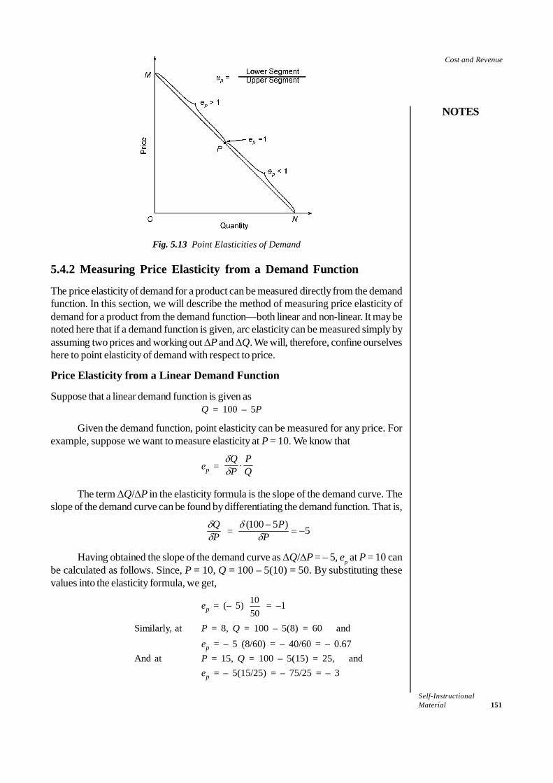
Self-InstructionalMaterial 151
Cost and Revenue
NOTES
Fig. 5.13 Point Elasticities of Demand
5.4.2 Measuring Price Elasticity from a Demand Function
The price elasticity of demand for a product can be measured directly from the demandfunction. In this section, we will describe the method of measuring price elasticity ofdemand for a product from the demand function—both linear and non-linear. It may benoted here that if a demand function is given, arc elasticity can be measured simply byassuming two prices and working out ΔP and ΔQ. We will, therefore, confine ourselveshere to point elasticity of demand with respect to price.
Price Elasticity from a Linear Demand Function
Suppose that a linear demand function is given asQ = 100 – 5P
Given the demand function, point elasticity can be measured for any price. Forexample, suppose we want to measure elasticity at P = 10. We know that
ep = QP
PQ⋅δ
δ
The term ΔQ/ΔP in the elasticity formula is the slope of the demand curve. Theslope of the demand curve can be found by differentiating the demand function. That is,
PQδδ
= 5)5100(−=
−P
Pδ
δ
Having obtained the slope of the demand curve as ΔQ/ΔP = – 5, ep at P = 10 canbe calculated as follows. Since, P = 10, Q = 100 – 5(10) = 50. By substituting thesevalues into the elasticity formula, we get,
ep = (– 5) 1050
= –1
Similarly, at P = 8, Q = 100 – 5(8) = 60 andep = – 5 (8/60) = – 40/60 = – 0.67
And at P = 15, Q = 100 – 5(15) = 25, andep = – 5(15/25) = – 75/25 = – 3

Self-Instructional152 Material
Cost and Revenue
NOTES
Price Elasticity from a Non-linear Demand Function
Suppose a non-linear demand function of multiplicative form is given as follows.Q = aP–b
and we want to compute the price elasticity of demand. The formula for computing theprice elasticity is the same, i.e.,
ep = QP
PQ⋅δ
δ …(5.25)
What we need to compute the price-elasticity coefficient is to find first the valueof the first term, ΔQ/ΔP, i.e., the slope of the demand curve. The slope can be obtainedby differentiating the demand function, Thus,
PQδδ
= – baP–b-1 …(5.26)
By substituting Eq. (5.26) in Eq. (5.25), ep can be expressed as
ep = – baP–b–1 PQ
⎛ ⎞⎜ ⎟⎝ ⎠
= bbaP
Q
−−…(5.27)
Since Q = aP–b, by substitution, we get
ep = b
b
baPaP
−
−
− = –b …(5.28)
Equation (5.28) shows that when a demand function is of a multiplicative or powerform, price elasticity coefficient equals the power of the variable P. This means thatprice elasticity in the case of a multiplicative demand function remains constant all alongthe demand curve regardless of a change in price.
5.4.3 Price Elasticity and Total Revenue
A firm aiming at enhancing its total revenue would like to know whether increasing ordecreasing the price would achieve its goal. The price-elasticity coefficient of demandfor its product at different levels of its price provides the answer to this question. Thesimple answer is that if ep > 1, then decreasing the price will increase the total revenueand if eq < 1, then increasing the price will increase the total revenue. To prove this point,we need to know the total revenue (TR) and the marginal revenue (MR) functions andmeasures of price-elasticity are required. Since TR = Q.P, we need to know P and Q.This information can be obtained through the demand function.
Q = 100 – 5P
Price function (P) can be derived from the demand function asP = 20 – 0.2Q …(5.29)
Given the price function, TR can be obtained asTR = P . Q = (20 – 0.2Q)Q = 20Q – 0.2Q2
From this TR-function, the MR-function can be derived as
MR = QTR∂∂
= 20 – 0.4Q

Self-InstructionalMaterial 153
Cost and Revenue
NOTES
The TR-function is graphed in panel (a) and the demand and MR functions arepresented in panel (b) of Figure 5.14. As the figure shows, at point P on the demandcurve, e = 1 where output, Q = 50. Below point P, e < 1 and above point P, e > 1. Itcan be seen in panel (a) of Figure 5.14 that TR increases so long as e > 1; TR reachesits maximum level where e = 1; and it decreases when e < 1.
Fig. 5.14 Price Elasticity and Total Revenue
The relationship between price-elasticity and TR is summed up in Table 5.3. Asthe table shows, when demand is perfectly inelastic (i.e., ep = 0 as is the case of avertical demand line) there is no decrease in quantity demanded when price is raised andvice versa. Therefore, a rise in price increases the total revenue and vice versa.
In case of an inelastic demand (i.e., ep < 1), quantity demanded increases byless than the proportionate decrease in price and hence the total revenue falls whenprice falls. The total revenue increases when price increases because quantity demandeddecreases by less than the proportionate increase in price.
If demand for a product is unit elastic (ep = 1) quantity demanded increases (ordecreases) in the proportion of decrease (or increase) in the price. Therefore, totalrevenue remains unaffected.
If demand for a commodity has ep > 1, change in quantity demanded is greaterthan the proportionate change in price. Therefore, the total revenue increases whenprice falls and vice versa.
The case of infinitely elastic demand represented by a horizontal straight line israre. Such a demand line implies that a consumer has the opportunity to buy any quantityof a commodity and the seller can sell any quantity of a commodity, at a given price. It is
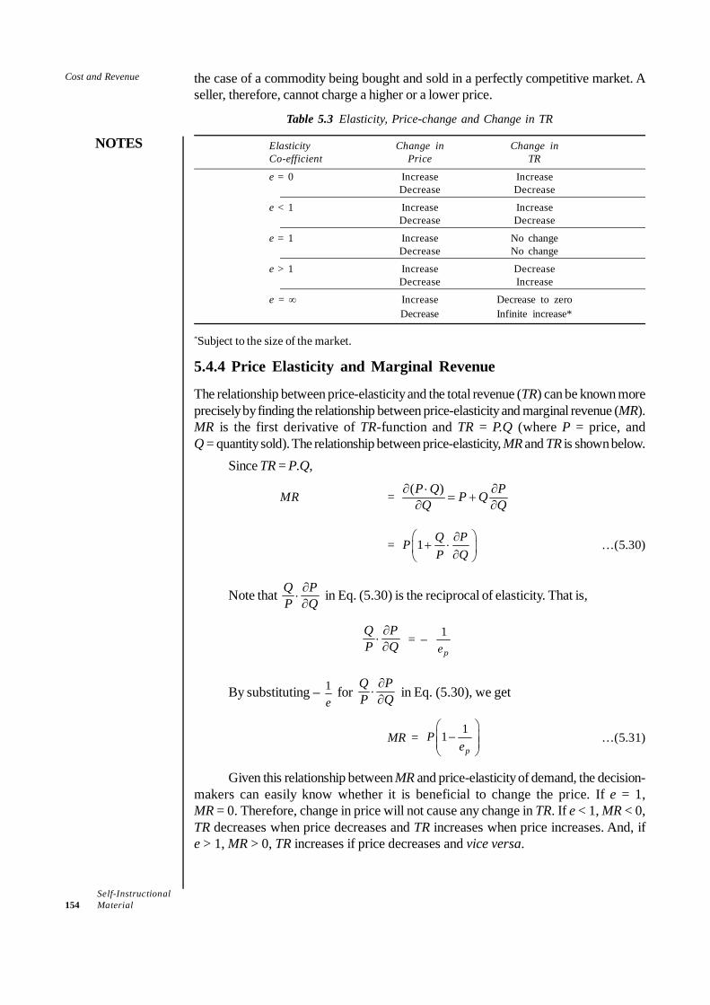
Self-Instructional154 Material
Cost and Revenue
NOTES
the case of a commodity being bought and sold in a perfectly competitive market. Aseller, therefore, cannot charge a higher or a lower price.
Table 5.3 Elasticity, Price-change and Change in TR
Elasticity Change in Change inCo-efficient Price TR
e = 0 Increase IncreaseDecrease Decrease
e < 1 Increase IncreaseDecrease Decrease
e = 1 Increase No changeDecrease No change
e > 1 Increase DecreaseDecrease Increase
e = ∞ Increase Decrease to zeroDecrease Infinite increase*
*Subject to the size of the market.
5.4.4 Price Elasticity and Marginal Revenue
The relationship between price-elasticity and the total revenue (TR) can be known moreprecisely by finding the relationship between price-elasticity and marginal revenue (MR).MR is the first derivative of TR-function and TR = P.Q (where P = price, andQ = quantity sold). The relationship between price-elasticity, MR and TR is shown below.
Since TR = P.Q,
MR = QPQPQ
QP∂∂
+=∂⋅∂ )(
= 1 Q PPP Q
⎛ ⎞∂+ ⋅⎜ ⎟∂⎝ ⎠
…(5.30)
Note that QP
PQ
∂∂⋅ in Eq. (5.30) is the reciprocal of elasticity. That is,
QP
PQ
∂∂⋅ = – 1
ep
By substituting – 1e
for QP
PQ
∂∂⋅ in Eq. (5.30), we get
MR = 11p
Pe
⎛ ⎞−⎜ ⎟⎜ ⎟
⎝ ⎠…(5.31)
Given this relationship between MR and price-elasticity of demand, the decision-makers can easily know whether it is beneficial to change the price. If e = 1,MR = 0. Therefore, change in price will not cause any change in TR. If e < 1, MR < 0,TR decreases when price decreases and TR increases when price increases. And, ife > 1, MR > 0, TR increases if price decreases and vice versa.
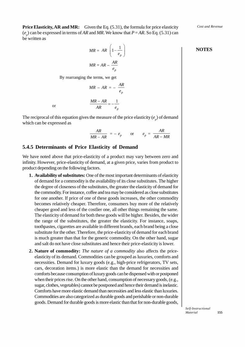
Self-InstructionalMaterial 155
Cost and Revenue
NOTES
Price Elasticity, AR and MR: Given the Eq. (5.31), the formula for price elasticity(ep) can be expressed in terms of AR and MR. We know that P = AR. So Eq. (5.31) canbe written as
MR = 11p
ARe
⎛ ⎞−⎜ ⎟⎜ ⎟
⎝ ⎠
MR = AR – p
ARe
By rearranging the terms, we get
MR – AR = – p
ARe
or1
p
MR ARAR e−
= −
The reciprocal of this equation gives the measure of the price elasticity (ep) of demandwhich can be expressed as
ARMR AR−
= – ep or ep = AR
AR MR−
5.4.5 Determinants of Price Elasticity of Demand
We have noted above that price-elasticity of a product may vary between zero andinfinity. However, price-elasticity of demand, at a given price, varies from product toproduct depending on the following factors.
1. Availability of substitutes: One of the most important determinants of elasticityof demand for a commodity is the availability of its close substitutes. The higherthe degree of closeness of the substitutes, the greater the elasticity of demand forthe commodity. For instance, coffee and tea may be considered as close substitutesfor one another. If price of one of these goods increases, the other commoditybecomes relatively cheaper. Therefore, consumers buy more of the relativelycheaper good and less of the costlier one, all other things remaining the same.The elasticity of demand for both these goods will be higher. Besides, the widerthe range of the substitutes, the greater the elasticity. For instance, soaps,toothpastes, cigarettes are available in different brands, each brand being a closesubstitute for the other. Therefore, the price-elasticity of demand for each brandis much greater than that for the generic commodity. On the other hand, sugarand salt do not have close substitutes and hence their price-elasticity is lower.
2. Nature of commodity: The nature of a commodity also affects the price-elasticity of its demand. Commodities can be grouped as luxuries, comforts andnecessities. Demand for luxury goods (e.g., high-price refrigerators, TV sets,cars, decoration items.) is more elastic than the demand for necessities andcomforts because consumption of luxury goods can be dispensed with or postponedwhen their prices rise. On the other hand, consumption of necessary goods, (e.g.,sugar, clothes, vegetables) cannot be postponed and hence their demand is inelastic.Comforts have more elastic demand than necessities and less elastic than luxuries.Commodities are also categorized as durable goods and perishable or non-durablegoods. Demand for durable goods is more elastic than that for non-durable goods,
Self-Instructional156 Material
Cost and Revenue
NOTES
because when the price of the former increases, people either get the old onerepaired instead of replacing it or buy a ‘second hand’.
3. Weightage in the total consumption: Another factor that influences theelasticity of demand is the proportion of income which consumers spend on aparticular commodity. If proportion of income spent on a commodity is large, itsdemand will be more elastic. On the contrary, if the proportion of income spent ona commodity is small, its demand is less price-elastic. Classic examples of suchcommodities are salt, matches, books, pens, toothpastes, etc. These goods claima very small proportion of income. Demand for these goods is generally inelasticbecause increase in the price of such goods does not substantially affect theconsumer’s budget. Therefore, people continue to purchase almost the samequantity even when their prices increase.
4. Time factor in adjustment of consumption pattern: Price-elasticity of demanddepends also on the time consumers need to adjust their consumption patternto a new price: the longer the time available, the greater the price-elasticity. Thereason is that over a period of time, consumers are able to adjust their expenditurepattern to price changes. For instance, if the price of TV sets is decreased, demandwill not increase immediately unless people possess excess purchasing power.But over time, people may be able to adjust their expenditure pattern so that theycan buy a TV set at a lower (new) price. Consider another example. If price ofpetrol is reduced, the demand for petrol does not increase immediately andsignificantly. Over time, however, people get incentive from low petrol prices tobuy automobiles resulting in a significant rise in demand for petrol.
5. Range of commodity use: The range of uses of a commodity also influencesthe price-elasticity of its demand. The wider the range of the uses of a product,the higher the elasticity of demand for the decrease in price. As the price of amulti-use commodity decreases, people extend their consumption to its other uses.Therefore, the demand for such a commodity generally increases more than theproportionate increase in its price. For instance, milk can be taken as it is and inthe form of curd, cheese, ghee and butter-milk. The demand for milk will thereforebe highly elastic for decrease in price. Similarly, electricity can be used for lighting,cooking, heating and for industrial purposes. Therefore, demand for electricityhas a greater elasticity. However, for the increase in price, such commoditieshave a lower price-elasticity because the consumption of a normal good cannotbe cut down substantially beyond a point when the price of the commodityincreases.
6. Proportion of market supplied: The elasticity of market demand also dependson the proportion of the market supplied at the ruling price. If less than halfof the market is supplied at the ruling price, price-elasticity of demand will behigher than 1 and if more than half of the market is supplied, e < 1.
5.4.6 Cross-Elasticity of Demand
The cross-elasticity is the measure of responsiveness of demand for a commodity to thechanges in the price of its substitutes and complementary goods. For instance, cross-elasticity of demand for tea is the percentage change in its quantity demanded withrespect to the change in the price of its substitute, coffee. The formula for measuringcross-elasticity of demand for tea (et, c) and the same for coffee (ec, t) is given below.
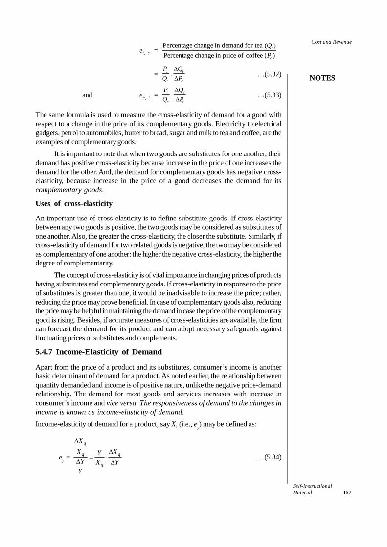
Self-InstructionalMaterial 157
Cost and Revenue
NOTES
et, c = Percentage change in demand for tea ( )Percentage change in price of coffee ( )
t
c
QP
= .c t
t c
P QQ P
ΔΔ
…(5.32)
and ec, t = .t c
c t
P QQ P
ΔΔ
…(5.33)
The same formula is used to measure the cross-elasticity of demand for a good withrespect to a change in the price of its complementary goods. Electricity to electricalgadgets, petrol to automobiles, butter to bread, sugar and milk to tea and coffee, are theexamples of complementary goods.
It is important to note that when two goods are substitutes for one another, theirdemand has positive cross-elasticity because increase in the price of one increases thedemand for the other. And, the demand for complementary goods has negative cross-elasticity, because increase in the price of a good decreases the demand for itscomplementary goods.
Uses of cross-elasticity
An important use of cross-elasticity is to define substitute goods. If cross-elasticitybetween any two goods is positive, the two goods may be considered as substitutes ofone another. Also, the greater the cross-elasticity, the closer the substitute. Similarly, ifcross-elasticity of demand for two related goods is negative, the two may be consideredas complementary of one another: the higher the negative cross-elasticity, the higher thedegree of complementarity.
The concept of cross-elasticity is of vital importance in changing prices of productshaving substitutes and complementary goods. If cross-elasticity in response to the priceof substitutes is greater than one, it would be inadvisable to increase the price; rather,reducing the price may prove beneficial. In case of complementary goods also, reducingthe price may be helpful in maintaining the demand in case the price of the complementarygood is rising. Besides, if accurate measures of cross-elasticities are available, the firmcan forecast the demand for its product and can adopt necessary safeguards againstfluctuating prices of substitutes and complements.
5.4.7 Income-Elasticity of Demand
Apart from the price of a product and its substitutes, consumer’s income is anotherbasic determinant of demand for a product. As noted earlier, the relationship betweenquantity demanded and income is of positive nature, unlike the negative price-demandrelationship. The demand for most goods and services increases with increase inconsumer’s income and vice versa. The responsiveness of demand to the changes inincome is known as income-elasticity of demand.Income-elasticity of demand for a product, say X, (i.e., ey) may be defined as:
ey =
q
q q
q
XX XY
Y X YY
Δ
Δ= ⋅
Δ Δ…(5.34)

Self-Instructional158 Material
Cost and Revenue
NOTES
(where Xq = quantity of X demanded; Y = disposable income; ΔXq = change in quantityof X demanded; and ΔY = change in income)
Obviously, the formula for measuring income-elasticity of demand is the sameas that for measuring the price-elasticity. The only change in the formula is that thevariable ‘income’ (Y) is substituted for the variable ‘price’ (P). Here, income refers tothe disposable income, i.e., income net of taxes. All other formulae for measuringprice-elasticities may by adopted to measure the income-elasticities, keeping in mindthe difference between them and the purpose of measuring income-elasticity.
To estimate income-elasticity, suppose, for example, government announces a10 per cent dearness allowance to its employees. As a result average monthly salary ofgovernment employees increases from ̀ 20,000 to ̀ 22,000. Following the pay-hike,monthly petrol consumption of government employees increases from 150 litre per monthto 165 litre. The income-elasticity of petrol consumption can now be worked out asfollows. In this case, ΔY = ̀ 22,000 – ̀ 20,000 = ̀ 2,000, and ΔQ (oil demand) = 165 litre– 150 litre = 15 litre. By substituting those values in Eq. (5.34), we get
ey = 20,000 15 1
150 2,000× =
It means that income elasticity of petrol consumption by government employeesequals 1. It means that a one per cent increase in income results in a one per centincrease in petrol consumption.
Unlike price-elasticity of demand, which is always negative,7 income-elasticity ofdemand is always positive8 because of a positive relationship between income and quantitydemanded of a product. But there is an exception to this rule. Income-elasticity ofdemand for an inferior good is negative, because of the inverse substitution effect. Thedemand for inferior goods decreases with increase in consumer’s income. The reason isthat when income increases, consumers switch over to the consumption of superiorsubstitutes, i.e., they substitute superior goods for inferior ones. For instance, whenincome rises, people prefer to buy more of rice and wheat and less of inferior foodgrains;non-vegetarians buy more of meat and less of potato, and travellers travel more by planeand less by train.
Nature of Commodity and Income-Elasticity
For all normal goods, income-elasticity is positive though the degree of elasticity variesin accordance with the nature of commodities. Consumer goods of the three categories,viz., necessities, comforts and luxuries have different elasticities. The general pattern ofincome-elasticities of different goods for increase in income and their effect on salesare given in Table 5.4.
Table 5.4 Income-Elasticities
Consumer goods Co-efficient of Effect on sales with changeincome-elasticity in income
1. Essential goods Less than one (ey < 1) Less than proportionatechange in sale
2. Comforts Almost equal to unity Almost proportionate(ey ≅ 1) change in sale
3. Luxuries Greater than unity More than proportionate(ey > 1) increase in sale
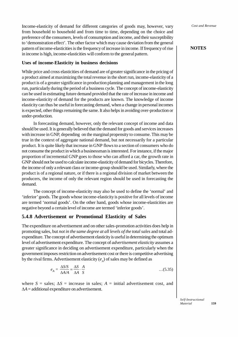
Self-InstructionalMaterial 159
Cost and Revenue
NOTES
Income-elasticity of demand for different categories of goods may, however, varyfrom household to household and from time to time, depending on the choice andpreference of the consumers, levels of consumption and income, and their susceptibilityto ‘demonstration effect’. The other factor which may cause deviation from the generalpattern of income-elasticities is the frequency of increase in income. If frequency of risein income is high, income-elasticities will conform to the general pattern.
Uses of income-Elasticity in business decisions
While price and cross elasticities of demand are of greater significance in the pricing ofa product aimed at maximizing the total revenue in the short run, income-elasticity of aproduct is of a greater significance in production planning and management in the longrun, particularly during the period of a business cycle. The concept of income-elasticitycan be used in estimating future demand provided that the rate of increase in income andincome-elasticity of demand for the products are known. The knowledge of incomeelasticity can thus be useful in forecasting demand, when a change in personal incomesis expected, other things remaining the same. It also helps in avoiding over-production orunder-production.
In forecasting demand, however, only the relevant concept of income and datashould be used. It is generally believed that the demand for goods and services increaseswith increase in GNP, depending on the marginal propensity to consume. This may betrue in the context of aggregate national demand, but not necessarily for a particularproduct. It is quite likely that increase in GNP flows to a section of consumers who donot consume the product in which a businessman is interested. For instance, if the majorproportion of incremental GNP goes to those who can afford a car, the growth rate inGNP should not be used to calculate income-elasticity of demand for bicycles. Therefore,the income of only a relevant class or income-group should be used. Similarly, where theproduct is of a regional nature, or if there is a regional division of market between theproducers, the income of only the relevant region should be used in forecasting thedemand.
The concept of income-elasticity may also be used to define the ‘normal’ and‘inferior’ goods. The goods whose income-elasticity is positive for all levels of incomeare termed ‘normal goods’. On the other hand, goods whose income-elasticities arenegative beyond a certain level of income are termed ‘inferior goods’.
5.4.8 Advertisement or Promotional Elasticity of Sales
The expenditure on advertisement and on other sales-promotion activities does help inpromoting sales, but not in the same degree at all levels of the total sales and total ad-expenditure. The concept of advertisement elasticity is useful in determining the optimumlevel of advertisement expenditure. The concept of advertisement elasticity assumes agreater significance in deciding on advertisement expenditure, particularly when thegovernment imposes restriction on advertisement cost or there is competitive advertisingby the rival firms. Advertisement elasticity (eA) of sales may be defined as
eA = S/S S AA/A A S
Δ Δ= ⋅
Δ Δ…(5.35)
where S = sales; ΔS = increase in sales; A = initial advertisement cost, andΔA = additional expenditure on advertisement.

Self-Instructional160 Material
Cost and Revenue
NOTES
Suppose, for example, a company increases its advertising expenditure from` 10 million to ̀ 20 million, and as a result, its sales increase from 50,000 units to 60,000units. In this case ΔA = 20 million – 10 million = ` 10 million, and ΔS = 60,000 –50,000 = 1000 units. By substituting these values in ad-elasticity formula (5.35), we get
eA = 10,000 10 0.2
10 50,000× =
It means that a one per cent increase in ad-expenditure results in only0.2 per cent increase in sales.Interpretation of advertisement elasticity: The advertisement elasticity of salesvaries between eA = 0 and eA = ∞. Interpretation of some measures of advertisingelasticity is given below.Elasticities Interpretation
eA = 0 Sales do not respond to the advertisement expenditure.eA > 0 but < 1 Increase in total sales is less than proportionate to the increase in
advertisement expenditure.eA = 1 Sales increase in proportion to the increase in expenditure on
advertisement.eA > Sales increase at a higher rate than the rate of increase of
advertisement expenditure.
Determinants of Advertisement Elasticity
Some important factors that determine ad-elasticity are the following.(i) The level of total sales: In the initial stages of sale of a product, particularly of
one which is newly introduced in the market, advertisement elasticity is greaterthan unity. As sales increase, ad-elasticity decreases. For instance, after thepotential market is supplied, the function of advertisement is to create additionaldemand by attracting more consumers to the product, particularly those who areslow in adjusting their consumption expenditure to provide for new commodities.Therefore, demand increases at a rate lower than the rate of increase inadvertisement expenditure.
(ii) Advertisement by rival firms: In a highly competitive market, the effectivenessof advertisement by a firm is also determined by the relative effectiveness ofadvertisement by the rival firms. Simultaneous advertisement by the rival firmsreduces sales of sales by a firm.
(iii) Cumulative effect of past advertisement: In case expenditure incurred onadvertisement in the initial stages is not adequate enough to be effective, elasticitymay be very low. But over time, additional doses of advertisement expendituremay have a cumulative effect on the promotion of sales and advertising elasticitymay increase considerably.
(iv) Other factors: Advertisement elasticity is affected also by other factors affectingthe demand for a product, e.g., change in products’ price, consumers’ income andgrowth of substitutes and their prices.
Self-InstructionalMaterial 161
Cost and Revenue
NOTES
5.4.9 Elasticity of Price Expectations
Sometimes, mainly during the period of price fluctuations, consumer’s price expectationsplay a much more important role than any other factor in determining the demand for acommodity. The concept of price-expectation-elasticity was devised and popularized byJ.R. Hicks in 1939. The price-expectation-elasticity refers to the expected change infuture price as a result of change in current prices of a product. The elasticity of price-expectation is defined and measured by the formula given below.
ex = //
f f f c
c c c f
P P P PP P P P
Δ Δ= ⋅
Δ Δ…(5.36)
where Pc and Pf are current and future prices respectively.The coefficient ex gives the measure of expected percentage change in future
price as a result of 1 per cent change in present price. If ex > 1, it indicates that futurechange in price will be greater than the present change in price, and vice versa. If ex =1, it indicates that the future change in price will be proportionately equal to the changein the current price.
The concept of elasticity of price-expectation is very useful in formulating futurepricing policy. For example, if ex > 1, it indicates that sellers will be able to sell more inthe future at higher prices. Thus, businessmen may accordingly determine their futurepricing policy.
5.5 SUMMARY
• The cost concepts that are relevant to business operations and decisions can begrouped on the basis of their nature and purpose under two overlapping categories:(i) cost concepts used for accounting purposes, and (ii) analytical cost conceptsused in economic analysis of business activities.
• The opportunity cost may be defined as the expected returns from the secondbest use of the resources that are foregone due to the scarcity of resources. Theopportunity cost is also called alternative cost.
• Business costs include all the expenses that are incurred to carry out a business.• The concept of full cost includes business costs, opportunity cost and normal
profit.• The opportunity cost includes the foregone expected earnings from the second
best use of the resources, or the market rate of interest on the total money capitaland also the value of an entrepreneur’s own services that are not charged for inthe current business.
• Actual or explicit costs are those which are actually incurred by the firm in paymentfor labour, material, plant, building, machinery, equipment, travelling and transport,advertisement.
• In contrast to explicit costs, there are some other costs that do not take the formof cash outlays, nor do they appear in the accounting system. Such costs areknown as implicit or imputed costs.
• The items of expenditure that involve cash payments or cash transfers, bothrecurring and non-recurring, are known as out-of-pocket costs.
Check Your Progress
10. Define elasticity ofdemand.
11. What is priceelasticity ofdemand?
12. Define arcelasticity.
13. What is incomeelasticity?
14. Define crosselasticity.
Self-Instructional162 Material
Cost and Revenue
NOTES
• There are certain actual business costs that do not involve cash payments, but aprovision is therefore made in the books of account and they are taken into accountwhile finalizing the profit and loss accounts. Such expenses are known as bookcosts.
• Fixed costs are those that are fixed in volume for a certain quantity of output.Variable costs are those which vary with the variation in the total output.
• Total cost (TC) is the total actual cost incurred on the production of goods andservice.
• Average cost (AC) is obtained by dividing the total cost (TC) by the total output(Q).
• Marginal cost (MC) is defined as the addition to the total cost on account ofproducing one additional unit of the product.
• Sunk costs are those costs which are made once and for all and cannot be altered,increased or decreased, by varying the rate of output, nor can they be recovered.
• Historical cost refers to the cost incurred in past on the acquisition of productiveassets, e.g. land, building, machinery, etc., whereas replacement cost refers tothe outlay that has to be made for replacing an old asset. These concepts owetheir significance to the unstable nature of price behaviour.
• Private costs are those which are actually incurred or provided for by an individualor a firm on the purchase of goods and services from the market.
• Social costs on the other hand, refer to the total cost borne by the society due toproduction of a commodity.
• One objective of business firms is to minimize Average Cost of their product or,which is the same as, to optimize the output.
• The long-run average cost curve (LAC) is derived by combining the short-runaverage cost curves (SACs).
• The long-run marginal cost curve (LMC) is derived from the short-run marginalcost curves (SMCs).
• The degree of responsiveness of demand to the change in its determinants iscalled elasticity of demand.
• Price elasticity of demand is generally defined as the responsiveness orsensitiveness of demand for a commodity to the changes in its price.
• The measure of elasticity of demand between any two finite points on a demandcurve is known as arc elasticity.
• The cross-elasticity is the measure of responsiveness of demand for a commodityto the changes in the price of its substitutes and complementary goods.
• The responsiveness of demand to the changes in income is known as income-elasticity of demand.
• The concept of cross-elasticity is of vital importance in changing prices of productshaving substitutes and complementary goods.
• For all normal goods, income-elasticity is positive though the degree of elasticityvaries in accordance with the nature of commodities.
Self-InstructionalMaterial 163
Cost and Revenue
NOTES
• The concept of income-elasticity can be used in estimating future demand providedthat the rate of increase in income and income-elasticity of demand for the productsare known. The knowledge of income elasticity can thus be useful in forecastingdemand, when a change in personal incomes is expected, other things remainingthe same. It also helps in avoiding over-production or under-production.
• The concept of advertisement elasticity assumes a greater significance in decidingon advertisement expenditure, particularly when the government imposesrestriction on advertisement cost or there is competitive advertising by the rivalfirms.
5.6 KEY TERMS
• Opportunity cost: Opportunity cost may be defined as the expected returnsfrom the second best use of the resources that are foregone due to the scarcity ofresources.
• Total cost (TC): Total cost is the total actual cost incurred on the production ofgoods and service.
• Average cost (AC): Average cost is obtained by dividing the total cost (TC) bythe total output (Q).
• Marginal cost (MC): Marginal cost is defined as the addition to the total cost onaccount of producing one additional unit of the product.
• Total revenue (TR): Total revenue is the total income of a business and iscalculated by multiplying the quantity of goods sold by the price of the goods.
• Average revenue (AR): Average revenue refers to the revenue per unit ofoutput sold.
• Marginal revenue (MR): Marginal revenue is the additional revenue generatedfrom the sale of an additional unit of output.
• Elasticity of demand: The degree of responsiveness of demand to the changein its determinants is called elasticity of demand.
• Price elasticity: Price elasticity of demand is generally defined as theresponsiveness or sensitiveness of demand for a commodity to the changes in itsprice.
• Arc elasticity: The measure of elasticity of demand between any two finitepoints on a demand curve is known as arc elasticity.
• Cross elasticity: It is the measure of responsiveness of demand for a commodityto the changes in the price of its substitutes and complementary goods.
• Income elasticity: The responsiveness of demand to the changes in income isknown as income-elasticity of demand.
5.7 ANSWERS TO ‘CHECK YOUR PROGRESS’
1. Opportunity cost may be defined as the expected returns from the second bestuse of the resources that are foregone due to the scarcity of resources. Theopportunity cost is also called alternative cost.
Self-Instructional164 Material
Cost and Revenue
NOTES
2. Business costs include all the expenses that are incurred to carry out a business.3. The concept of full cost includes business costs, opportunity cost and normal
profit.4. Sunk costs are costs which are made once and for all and cannot be altered,
increased or decreased, by varying the rate of output, nor can they be recovered.5. Historical cost refers to the cost incurred in past on the acquisition of productive
assets, e.g. land, building, machinery6. (b) Cost fixed in volume for a certain quantity of output7. (c) Incremental costs are closely related to the concept of marginal cost but with
a relatively wider connotation8. One objective of business firms is to minimize average cost (AC) of their product
or, which is the same as, to optimize the output.9. When Average Fixed Cost (AFC) falls but Average Variable Cost (AVC) increases,
change in Average Cost (AC) depends on the rate of change in Average FixedCost (AFC) and Average Variable Cost (AVC):• If decrease in AFC > increase in AVC, then AC falls,• If decrease in AFC = increase in AVC, AC remains constant, and• If decrease in AFC < increase in AVC, then AC increase
10. The degree of responsiveness of demand to the change in its determinants iscalled elasticity of demand.
11. Price elasticity of demand is generally defined as the responsiveness orsensitiveness of demand for a commodity to the changes in its price.
12. The measure of elasticity of demand between any two finite points on ademandcurve is known as arc elasticity.
13. The cross-elasticity is the measure of responsiveness of demand for a commodityto the changes in the price of its substitutes and complementary goods.
14. The responsiveness of demand to the changes in income is known as income-elasticity of demand.
5.8 QUESTIONS AND EXERCISES
Short-Answer Questions
1. Distinguish between out-of pocket and book costs.2. Differentiate between explicit and implicit costs.3. Distinguish between private and social costs.4. Distinguish between total, marginal and average revenue.5. What are the uses of cross-elasticity?6. How does nature of commodities affect income elasticity?
Long-Answers Questions
1. Discuss the relationship between total, average and marginal costs.2. Explain law of diminishing returns with the help of cost curves.

Self-InstructionalMaterial 165
Cost and Revenue
NOTES
3. Illustrate graphically optimization of output in the short-run and long-run cost-output relations.
4. Discuss the relationship between price elasticity and total revenue, marginal andaverage revenue.
5. What are the determinants of price elasticity of demand?6. What are the uses of income elasticity in business decisions? Discuss the
determinants of advertisement elasticity.
5.9 FURTHER READING/ENDNOTES
Varshney and Maheshwari. 2011. Managerial Economics. New Delhi: Sultan Chandand Sons.
Mankar, V. G. 1982. Business Economics. New Delhi: Himalya Publishing House.Dufty, N.F. 1966. Managerial Economics. New York: Asia Publishing House.
Endnotes
1. Watson, Donald S., Price Theory and Its Uses, Houghton Mifflin Company, Boston,1963, p. 126.
2. Dean, Joel, Managerial Economics, op. cit., p. 262.3. There may be some nominal payment for the use of public utilities in the form of
tax, which may not cover the full cost thereof.4. Mansfield, Edwin, op. cit., p. 525. The elasticity formula is derived as follows:
1
1
1
1
1
21
1
21
100
100
QP
PQ
PP
PPP
QQQ
ep ⋅ΔΔ
=Δ
Δ
=×
−
×−
=
where P1 is old price, P2 is new price Q1 is quantity demanded at P1 and Q2 isquantity demanded at P2.
6. Price-elasticity of demand calculated without a minus sign will always be a negativevalue because either ΔP or ΔQ will carry a negative sign due to inverse relationshipbetween price and quantity demanded. This gives a negative value of elasticity whereasin the concept of elasticity, a negative value has no meaningful interpretation expectthat it indicates inverse relationship between P and Q. The negative elasticitycoefficient is rather misleading. The ‘minus’ sign is, therefore, inserted as a matterof ‘linguistic’ convenience, to make the coefficient of elasticity non-negative.Sometimes, ‘it is also suggested to ignore the negative sign in the numerator anddenominator of the elasticity formula. The elasticity in Eq. (5.19) ignores the negativesign.
7. Except in case of Giffen’s goods.8. With the exception of inferior goods.

Self LearningMaterial 167
Pricing
NOTES
UNIT 6 PRICING
Structure6.0 Introduction6.1 Unit Objectives6.2 Objectives of the Firm
6.2.1 Profit Maximization6.2.2 Sales Revenue Maximization
6.3 Pricing Under Different Market Structures6.3.1 Perfect Competion6.3.2 Monopoly6.3.3 Price Discrimination Under Monopoly6.3.4 Price Discrimination by Degrees
6.4 Product Line Pricing6.4.1 Joint Product Pricing
6.5 Summary6.6 Key Terms6.7 Answers to ‘Check Your Progress’6.8 Questions and Exercises6.9 Further Reading/Endnotes
6.0 INTRODUCTION
The first and most important responsibility of a business manager is to achieve theobjective of the firm he manages. However, as we will see, the objectives of businessfirms can be varied and also conflicting. The primary objective of a business firm is tomake profit. That is why the conventional theory of firm assumes profit maximization—not just making any profit—as the sole objective of business firms. Recent researcheson this issue reveal that the objectives business firms pursue are more than one. Someimportant objectives, other than profit maximization, are: (a) maximization of sales revenue,(b) maximization of firm’s growth rate, (c) maximization of manager’s utility function,(d) making a satisfactory rate of profit, (e) long-run survival of the firm, and (f) entry-prevention and risk-avoidance. Although the conventional theory of firm still holds itsground firmly, several alternative theories of firm were proposed during the early 1960sby economists, notably by Simon, Baumol, Marris, Williamson, Berle and Means, Galbraith,and Cyert and March. There are now a number of alternative theories of firms postulatingdifferent objectives of business firms.
Maximization of output or minimization of cost or optimization of resource allocationis, however, only one aspect of the profit maximizing behaviour of the firm. Another andequally important aspect of profit maximization is to find the price from the set of pricesrevealed by the demand schedule that is in agreement with profit maximization objectiveof the firm. The level of profit-maximizing price is generally different in different kindsof markets, depending on the degree of competition between the sellers. Therefore,while determining the price of its product, a firm has to take into account the nature ofthe market. In this chapter, we discuss the theory of price determination and also thefirm’s equilibrium in various kinds of market structures.
In a complex business world, business firms follow a variety of pricing rules andmethods depending on the conditions faced by them. In this chapter, we will discusssome important pricing strategies and pricing practices as discovered by the economists.
Self Learning168 Material
Pricing
NOTES
6.1 UNIT OBJECTIVES
After going through this unit, you will be able to:• Understand the objectives of a firm and theories that analyse a firm’s behaviour• Discuss pricing under different market structures• Explain product-line pricing and joint product pricing
6.2 OBJECTIVES OF THE FIRM
Profit means different things to different people. ‘The word “profit” has different meaningto businessmen, accountants, tax collectors, workers and economists and it is often usedin a loose polemical sense that buries its real significance…’1 In a general sense, ‘profit’is regarded as income accruing to equity holders, in the same sense as wages accrue tolabour; rent accrues to owners of rentable assets; and interest accrues to themoneylenders. To a layman, profit means all income that flows to the investors. To anaccountant, ‘profit’ means the excess of revenue over all paid-out costs, including bothmanufacturing and overhead expenses. It is more or less the same as ‘net profit’. For allpractical purposes, profit (or business income) means profit in accountancy sense plusnon-allowable expenses.2 Profit figures published by the business firms are profitsconforming to accounting concept of profit. Economist’s concept of profit is of ‘pureprofit’, also called ‘economic profit’ or ‘just profit’. Pure profit is a return over andabove the opportunity cost, i.e., the income which a businessman might expect from thesecond best alternative use of his resources. These two concepts of profit are discussedbelow in detail.
The two important concepts of profit that figure in business decisions are ‘economicprofit’ and ‘accounting profit’. From conceptual clarity point of view, it is useful tounderstand the difference between the two concepts of profit. In accounting sense,profit is surplus of total revenue over and above all paid-out costs, including bothmanufacturing and overhead expenses. Accounting profit may be calculated as follows.
Accounting profit = TR – (W + R + I + M)where TR = Total revenue, W = wages and salaries, R = rent, I = interest,and M = cost of materialsObviously, while calculating accounting profit, only explicit or book costs, i.e., the
costs recorded in the books of accounts, are considered.The concept of ‘economic profit’ differs from ‘accounting profit’. Economic profit
also takes into account the implicit or imputed costs. The implicit cost is opportunity cost.Opportunity cost is defined as the payment that would be ‘necessary to drawforth thefactors of production from their most remunerative alternative employment’. Alternatively,opportunity cost can be defined as the income foregone which a businessman couldmake from the second best use of his resources. For example, if an entrepreneur useshis capital in his own business, he foregoes dividend which he could earn by purchasingshares of other companies or the interest which he could earn by depositing his moneywith banks for a period. Furthermore, if an entrepreneur uses his time and labour in hisown business, he foregoes his income (salary) which he could earn by working as amanager in another firm. Similarly, by using productive assests (land and building) in his
Self LearningMaterial 169
Pricing
NOTES
own business, he sacrifices his market rent. These foregone incomes—interest, salaryand rent—are called opportunity costs or transfer costs. Accounting profit does nottake into account the opportunity cost but economic profit does.
It should also be noted that economic or pure profit makes provision also for(a) insurable risks, (b) depreciation, and (c) necessary minimum payment to shareholdersto prevent them from withdrawing their capital. Pure profit may thus be defined as ‘aresidual left after all contractual costs have been met, including the transfer costs ofmanagement, insurable risks, depreciation and payments to shareholders sufficient tomaintain investment at its current level’. Thus,
Pure profit = Total revenue – (explicit costs + implicit costs)Alternatively, pure profit may be defined as follows.Pure profit = Accounting profit – (opportunity cost + unauthorized payments, e.g.,
bribes)Pure profit so defined may not be necessarily positive for a single firm in a single
year—it may be negative, since it may not be possible to decide beforehand the bestway of using the resources. Besides, in economics, pure profit is considered to be ashort-term phenomenon—it does not exist in the long run, especially under perfectlycompetitive market conditions.
6.2.1 Profit Maximization
Profit maximization has been the most important assumption on which economists havebuilt price and production theories. This assumption has, however, been strongly questionedand alternative hypotheses suggested. Let us look into the importance of the profitmaximization assumption and theoretical conditions of profit maximization.
The conventional economic theory assumes profit maximization as the onlyobjective of business firms. Profit maximization as the objective of business firms has along history in economic literature. It forms the basis of conventional price theory. Profitmaximization is regarded as the most reasonable and analytically the most ‘productive’business objective. The strength of this assumption lies in the fact that this assumption‘has never been unambiguously disproved’.
Besides, profit maximization assumption has a greater predictive power. It helpsin predicting the behaviour of business firms in the real world and also the behaviour ofprice and output under different market conditions. No alternative hypothesis explainsand predicts the behaviour of firms better than the profit maximization assumption. Letus now discuss the theoretical conditions for profit maximization.
Total profit (Π) is defined asΠ = TR – TC …(6.1)
where TR = total revenue, and TC = total cost.
There are two conditions that must be fulfilled for TR – TC to be maximum.These conditions are called (i) necessary or the first order condition, and(ii) secondary or supplementary condition.
Necessary or the first-order condition: Requires that marginal revenue (MR)must be equal to marginal cost (MC). By definition, marginal revenue is the revenueobtained from the production and sale of one additional unit of output and marginal costis the cost arising due to the production of one additional unit of output.

Self Learning170 Material
Pricing
NOTES
Secondary or the second-order condition: Requires that the necessary orfirst-order condition must be satisfied under the stipulation of decreasing MR and risingMC. The fulfilment of the two conditions makes it the sufficient condition.
The profit maximizing conditions can also be presented algebraically as follows.We know that a profit maximizing firm seeks to maximize
Π = TR – TC
Let us suppose that the total revenue (TR) and total cost (TC) functions are,respectively, given as
TR = f(Q) and TC = f(Q)where Q = quantity produced and sold.
By substituting total revenue and total cost functions in Eq. (6.1), the profit functionmay be written as
Π = f(Q)TR – f(Q)TC ...(6.2)
Equation (6.2) can now be manipulated to illustrate the first and second orderconditions of profit maximization as follows.
First-order condition: The first-order condition of maximizing a function is thatits first derivative must be equal to zero. Thus, the first-order condition of profit maximizationis that the first derivative of the profit function Eq. (6.2) must be equal to zero.Differentiating the total profit function and setting it equal to zero, we get
0TR TCQ Q Q
∂Π ∂ ∂= − =
∂ ∂ ∂...(6.3)
This condition holds only when
TR TCQ Q
∂ ∂=
∂ ∂
In Eq. (6.3), the term ∂TR/∂Q gives the slope of the TR curve which in turn givesthe marginal revenue (MR). Similarly, the term ∂TC/∂Q gives the slope of the total costcurve which is the same as marginal cost (MC). Thus, the first-order condition for profitmaximization can be stated as
MR = MC
The first-order condition is generally known as necessary condition. A necessarycondition is one that must be satisfied for an event to take place. In other words, thecondition that MR = MC must be satisfied for profit to be maximum.
Second-order condition: As already mentioned, in non-technical terms, thesecond-order condition of profit maximization requires that the first order condition issatisfied under rising MC and decreasing MR. This condition is illustrated in Figure 6.1.The MC and MR curves are the usual marginal cost and marginal revenue curvesrespectively. Incidentally, MC and MR curves are derived from TC and TR functionsrespectively. (The method of derivation has been shown later in the book). MC and MRcurves intersect at two points, P1 and P2. Thus, the firstorder condition is satisfied atboth the points, but the second order condition of profit maximization is satisfied only atpoint P2. Technically, the second-order condition requires that the second derivative ofthe profit function is negative. The second derivative of the total profit function is givenas

Self LearningMaterial 171
Pricing
NOTES
2
2
2
2
2
2
QTC
QTR
Q ∂∂
−∂∂
=∂
Π∂...(6.4)
Fig. 6.1 Marginal Conditions of Profit Maximization
The second-order condition requires that
02
2
2
2<
∂∂
−∂∂
QTC
QTR
or 2
2
2
2
QTC
QTR
∂∂
<∂∂
...(6.5)
Since ∂ 2TR/∂Q 2 gives the slope of MR and ∂ 2TC/∂Q2 gives the slope of MC,the second-order condition may also be written as
Slope of MR < Slope of MC
It implies that MC must have a steeper slope than MR or MC must intersect theMR from below.
To conclude, profit is maximized where both the first and second order conditionsare satisfied.
We may now apply the profit maximization conditions to a hypothetical exampleand compute profit maximizing output.
We know that TR = P.QSuppose demand function for a product is given as Q = 50 – 0.5P. Given the
demand function, price (P) function can be derived as
P = 100 – 2Q …(6.6)
By substituting price function for P in TR equation, we get
TR = (100 – 2Q)Q
or TR = 100Q – 2Q2 …(6.7)
Let us also suppose that the total cost function is given as
TC = 10 + 0.5 Q2 …(6.8)

Self Learning172 Material
Pricing
NOTES
Given the TR function (6.7) and TC function (6.8), we can now apply the firstorder condition of profit maximization and find profit maximizing output. We have notedthat profit is maximum where
MR = MC
or TR TCQ Q
∂ ∂=
∂ ∂
Given the total TR function in Eq. (6.7) and TC function in Eq. (6.8),
MR = TRQ
∂∂
= 100 – 4Q ...(6.9)
and MC = TCQ
∂∂
= Q ...(6.10)
Thus, profit is maximum whereMR = MC
or 100 – 4Q = Q
5Q = 100
Q = 20
The output 20 satisfies the second-order condition also. The second-ordercondition requires that
2 2
2 2 0TR TCQ Q
∂ ∂− <
∂ ∂
In other words, the second-order condition requires that
0MR MCQ Q
∂ ∂− <
∂ ∂
or (100 4 ) ( ) 0Q Q
Q Q∂ − ∂
− <∂ ∂
That is, – 4 – 1 < 0
Thus, the second-order condition is also satisfied at output 20.
6.2.2 Sales Revenue Maximization
Baumols’s theory of sales maximization is one of the most important alternative theoriesof firm’s behaviour. The basic premise of Baumol’s theory is that sales maximization,rather than profit maximization, is the plausible goal of the business firms. He arguesthat there is no reason to believe that all firms seek to maximize their profits. Businessfirms, in fact, pursue a number of incompatible objectives and it is not easy to single outone as the most common objective pursued by the firms. However, from his experienceas a consultant to many big business houses, Baumol finds that most managers seek tomaximize sales revenue rather than profits. He argues that, in modern business,management is separated from ownership, and managers enjoy the discretion to pursue

Self LearningMaterial 173
Pricing
NOTES
goals other than profit maximization. Their discretion eventually falls in favour of salesmaximization.
According to Baumol, business managers pursue the goal of sales maximizationfor the following reasons.
First, financial institutions consider sales as an index of performance of the firmand are willing to finance the firm with growing sales.
Secondly, while profit figures are available only annually at the end of the finalaccounting year, sales figures can be obtained easily and more frequently to assess theperformance of the management. Maximization of sales is more satisfying for themanagers than the maximization of profits that go into the pockets of the shareholders.
Thirdly, salaries and slack earnings of the top managers are linked more closelyto sales than to profit. Therefore, managers aim at maximizing sales revenue.
Fourthly, the routine personnel problems are more easily handled with growingsales. Higher payments may be offered to employees if sales figures indicate betterperformance. Profits are generally known after a year. To rely on profit figures means,therefore, a longer waiting period for both the employees and the management forresolving labour problems.
Fifthly, where profit maximization is the goal and it rises in one period to anunusually high level, this becomes the standard profit target for the shareholders thatmanagers find very difficult to maintain in the long run. Therefore, managers tend to aimat sales maximization rather than profit maximization.
Finally, sales growing at a rate higher than the rate of market expansion indicategrowing market share, a greater competitive strength and better bargaining power of afirm in a collusive oligopoly. In a competitive market, therefore, sales maximization isfound to be a more reasonable target.
To formulate his theory of sales maximization, Baumol3 has developed two basicmodels: (i) Static Model and (ii) Dynamic model—each with and without advertising.His static models with and without advertising are discussed below4.
Baumol’s Model without Advertising
Baumol assumes cost and revenue curves to be given as in conventional theory ofpricing. Suppose that the total cost (TC) and the total revenue (TR) curves are given asin Figure 6.2. The total profit curve, TP, is obtained by plotting the difference betweenthe TR and TC curves. Profits are zero where TR = TC.
Fig. 6.2 Sales Revenue Maximization

Self Learning174 Material
Pricing
NOTES
Given the TR and TC curves, there is a unique level of output at which total salesrevenue is maximum. The total sales revenue is maximum at the highest point of the TRcurve. At this point, slope of the TR curve (i.e., MR = ∂TR/∂Q) is equal to zero. Thehighest point on the TR curve can be obtained easily by drawing a line parallel to thehorizontal axis and tangent to the TR curve. The point H on the TR curve in Figure 6.2represents the total maximum sales revenue. A line drawn from point H to output axisshows that sales revenue is maximized at output OQ3. It implies that a sales revenuemaximizing firm will produce output OQ3 and its price equals HQ3/OQ3.
Profit Constraint and Revenue Maximization
At output OQ3, the firm maximizes its total revenue. At this output, the firm makes atotal profit equal to HQ3 – MQ3 = HM. Since total TP curve gives the measure of totalprofit at different levels of output, profit HM = TQ3. If this profit is enough or more thanenough to satisfy the stockholders, the firm will produce output OQ3 and charge a price= HQ/OQ3. But, if profit at output OQ3 is not enough to satisfy the stockholders, thenthe firm’s output must be changed to a level at which it makes a satisfactory profit, sayOQ2, which yields a profit LQ2 > TQ3.
Thus, there are two types of probable equilibrium—one in which the profit constraintdoes not provide an effective barrier to sales maximization,5 and second in which profitconstraint does provide an effective barrier to sales maximization. In the second type ofequilibrium, the firm will produce an output that yields a satisfactory or target profit. Itmay be any output between OQ1 and OQ2. For example, if minimum required profit isOP1, then the firm will stick to its sales maximization goal and produce output OQ3which yields a profit much greater than the required minimum. Since actual profit (TQ3)is much greater than the minimum required, the minimum profit constraint is not operative.
However, if required minimum profit level is OP2, OQ3 will not yield sufficientprofit to meet the profit target. The firm will, therefore, produce an output which yieldsthe required minimum level of profit OP2 (= LQ2). Given the profit target OP2, the firmwill produce OQ2 where its profit is just sufficient to meet requirement of minimumprofit. As can be seen in Figure 6.2, output (OQ2) is less than the sales maximizationoutput OQ3. Evidently, the profit maximization output, OQ1 is less than the salesmaximization output OQ2 (with profit constraint).
Baumol’s Model with Advertising
We have shown above how price and output are determined in a static single periodmodel without advertising. In an oligopolistic market structure, however, price and outputare subject to non-price competition. Baumol considers in his model with advertising asthe typical form of non-price competition and suggests that the various forms of non-price competition may be analyzed on similar lines.
In his analysis of advertising, Baumol makes the following assumptions.• Firm’s objective is to maximize sales, subject to a minimum profit constraint• Advertising causes a shift in the demand curve and hence the total sales
revenue (TR) rises with an increase in advertisement expen-diture (A) i.e.,∂TR/∂A > 0
• Price remains constant — a simplifying assumption• Production costs are independent of advertising. This is rather an unrea-
listic assumption since increase in sales may put output at a different coststructure.
Check Your Progress
1. Define pure profit.2. State the most
importantassumption of theconventionaleconomic theory.
3. State the basicpostulate ofBaumol’s theory.
4. Name the two basicmodels developedby Baumol.

Self LearningMaterial 175
Pricing
NOTES
Fig. 6.3 Sales Revenue Maximisation
Baumol’s model with advertising is presented in Figure 6.3. The TR and TC aremeasured on the Y-axis and total advertisement outlay on the X-axis. The TR curve isdrawn on the assumption that advertising increases total sales in the same manner asprice reduction.
The TC curve includes both production and advertisement costs. The total profitcurve is drawn by subtracting TC from TR. The profit so estimated is shown by thecurve PT. As shown in Figure 6.3 profit maximizing advertisement expenditure is OApwhich maximizes profit at MAp. Note that MAp = RC. Assuming that minimum profitrequired is OB, the sales maximizing advertisement outlay would be OAc. This impliesthat a firm increases its advertisement outlay until it reaches the target profit levelwhich is lower than the maximum profit. This also means that sales maximizers advertisenot less but more than the profit maximizers.
Criticism of Baumol’s Model
Although Baumol’s sales maximization model is found to be theoretically sound andempirically practicable, economists have pointed out the following shortcomings in hismodel.
First, it has been argued that in the long-run, Baumol’s sales maximization hypothesisand the conventional hypothesis would yield identical results, because the minimum requiredlevel of profits would coincide with the normal level of profits.
Second, Baumol’s theory does not distinguish between firm’s equilibrium andindustry equilibrium. Nor does it establish industry’s equilibrium when all the firms aresales maximizers.
Third, it does not clearly bring out the implications of interdependence of thefirm’s price and output decisions. Thus, Baumol’s theory ignores not only actual competitionbetween the firms but also the threat of potential competition in an oligopolistic market.
Fourth, Baumol’s claim that his solution is preferable to the solutions offered by theconventional theory, from a social welfare point of view, is not necessarily valid
6.3 PRICING UNDER DIFFERENT MARKETSTRUCTURES
The market structure determines a firm’s power to fix the price of its product a greatdeal. The degree of competition determines a firm’s degree of freedom in assessing theprice of its product. The degree of freedom implies the extent to which a firm is free or
Check Your Progress
5. Economic profit:(i) Is similar to
accounting profit(ii) Takes into
account theimplicit orimputed costs
(iii) Is a short-termphenomenon
(iv) Assumes profitmaximization asthe onlyobjective ofbusiness firms
6. According toBaumol's salesrevenuemaximizationtheory:(i) It is the most
reasonable andanalytically themost'productive'businessobjective
(ii) Most managersseek to maximizesales revenuerather thanprofits
(iii) No alternativehypothesisexplains andpredicts thebehaviour offirms better thanthe profitmaximizationassumption
(iv) Pure profit isconsidered to bea short-termphenomenon, itdoes not exist inthe long run
Self Learning176 Material
Pricing
NOTES
independent of the rival firms in taking its own pricing decisions. Depending on themarket structure, the degree of competition varies between zero and one. And, a firm’sdiscretion or the degree of freedom in setting the price for its product varies betweenone and none in the reverse order of the degree of competition. As a matter of rule, thehigher the degree of competition, the lower the firm’s degree of freedom in pricingdecision and control over the price of its own product and vice versa. Let us now seehow the degree of competition affects pricing decisions in different kinds of marketstructures.
Under perfect competition, a large number of firms compete against each otherfor selling their product. Therefore, the degree of competition under perfect competitionis close to one, i.e., the market is highly competitive. Consequently, firm’s discretion indetermining the price of its product is close to none. In fact, in perfectly competitivemarket, price is determined by the market forces of demand and supply and a firm hasto accept the price determined by the market forces. If a firm uses its discretion to fixthe price of its product above or below its market level, it loses its revenue and profit ineither case. For, if it fixes the price of its product above the ruling price, it will not be ableto sell its product, and if it cuts the price down below its market level, it will not be ableto cover its average cost. In a perfectly competitive market, therefore, firms have littleor no choice in respect to price determination.
As the degree of competition decreases, firm’s control over the price and itsdiscretion in pricing decision increases. For example, under monopolistic competition,where degree of competition is high but less than one, the firms have some discretion insetting the price of their products. Under monopolistic competition, the degree of freedomdepends largely on the number of firms and the level of product differentiation. Whereproduct differentiation is real, firm’s discretion and control over the price is fairly highand where product differentiation is nominal or only notional, firm’s pricing decision ishighly constrained by the prices of the rival products.
The control over the pricing discretion increases under oligopoly where degree ofcompetition is quite low, lower than that under monopolistic competition. The firms,therefore, have a good deal of control over the price of their products and can exercisetheir discretion in pricing decisions, especially where product differentiation is prominent.However, the fewness of the firms gives them an opportunity to form a cartel or to makesome settlement among themselves for fixation of price and non-price competition.
In case of a monopoly, the degree of competition is close to nil. An uncontrolledmonopoly firm has full control over the price of its product. A monopoly, in the true senseof the term, is free to fix any price for its product, of course, under certain constraints,viz., (i) the objective of the firm, and (ii) demand conditions.
The theory of pricing explains pricing decisions and pricing behaviour of the firmsin different kinds of market structures. In this chapter, we will describe the characteristicsof different kinds of market structures and price determination in each type of market ina theoretical framework. We begin with price determination under perfect competition.
6.3.1 Perfect Competion
The term perfect competition refers to a set of conditions prevailing in the market. Aperfectly competitive market is one which has the following characteristics.1. A large number of sellers and buyers: Under perfect competition, the number ofsellers and buyers is very large. The number of sellers is so large that the share of each

Self LearningMaterial 177
Pricing
NOTES
seller in total supply of a product is too small for a single seller to affect the market priceby changing his supply. Likewise, the number of buyers is so large that the share of eachbuyer in total demand is too small for a single buyer to influence the market price bychanging his/her demand.2. Homogeneous products: Products supplied by all firms are almost homogeneous.Homogeneity of products means that products supplied by various firms are so identicalin appearance and use that buyers do not distinguish between them nor do they preferthe product of one firm to that of another. Product of each firm is regarded as a perfectsubstitute for the product of other firms. Hence, no firm can gain any competitiveadvantage over the other firms. Nor do the firms distinguish between the buyers. Forexample, wheat and vegetables produced by all the farmers, other things given, aretreated as homogeneous.3. Perfect mobility of factors of production: For a market to be perfectly competitive,there should be perfect mobility of resources. This means that the factors of productionmust be in a position to move freely into or out of an industry and from one firm toanother. This is however a purely theoretical assumption.4. Free entry and free exit of firms: There is no barrier, legal or market-related, onthe entry of new firms into or exit of existing ones from the industry. Firms are free toenter the industry and quit it at their free will.5. Perfect knowledge: There is perfect dissemination of the information about themarket conditions. Both buyers and sellers are fully aware of the nature of the product,its availability or saleability and of the price prevailing in the market.6. Absence of collusion or artificial restraint: There is no sellers’ union or other kinds ofcollusions between the sellers such as cartels or guilds, nor is there any kind of collusionbetween the buyers, e.g., consumers’ associations or consumer forum. Each seller andbuyer acts independently. The firms enjoy the freedom of independent decisions.7. No government intervention: In a perfectly competitive market, there is nogovernment intervention with the working of the market system. There is no licencingsystem regulating the entry of firms to the industry, no regulation of market prices, i.e.,fixation of lower or upper limits of prices, no control over the supply of inputs, no fixationof quota on production, and no rationing of consumer demand, no subsidy to producersor to consumers, etc.
Perfect competition, as characterized above, is an uncommon phenomenon in thereal business world. However, the actual markets that approximate to the conditions ofperfectly competitive model include the share markets, securities and bond markets, andagricultural product markets, e.g., local vegetable markets. Although perfectly competitivemarkets are uncommon phenomena, perfect competition model has been the most popularmodel used in economic theories due to its analytical value as it provides a starting pointand analytical framework for pricing theory.
Perfect Competition and Pure Competition
Sometimes a distinction is made between perfect competition and pure competition. Thedifference between the two is only a matter of degree. Perfect competition less perfectmobility of factors and perfect knowledge is regarded as pure competition. In thisbook, however, we shall use the two terms interchangeably.
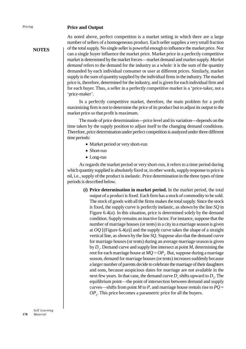
Self Learning178 Material
Pricing
NOTES
Price and Output
As noted above, perfect competition is a market setting in which there are a largenumber of sellers of a homogeneous product. Each seller supplies a very small fractionof the total supply. No single seller is powerful enough to influence the market price. Norcan a single buyer influence the market price. Market price in a perfectly competitivemarket is determined by the market forces—market demand and market supply. Marketdemand refers to the demand for the industry as a whole: it is the sum of the quantitydemanded by each individual consumer or user at different prices. Similarly, marketsupply is the sum of quantity supplied by the individual firms in the industry. The marketprice is, therefore, determined for the industry, and is given for each individual firm andfor each buyer. Thus, a seller in a perfectly competitive market is a ‘price-taker, not a‘price-maker’.
In a perfectly competitive market, therefore, the main problem for a profitmaximizing firm is not to determine the price of its product but to adjust its output to themarket price so that profit is maximum.
The mode of price determination—price level and its variation—depends on thetime taken by the supply position to adjust itself to the changing demand conditions.Therefore, price determination under perfect competition is analyzed under three differenttime periods:
• Market period or very short-run• Short-run• Long-run
As regards the market period or very short-run, it refers to a time period duringwhich quantity supplied is absolutely fixed or, in other words, supply response to price isnil, i.e., supply of the product is inelastic. Price determination in the three types of timeperiods is described below.
(i) Price determination in market period. In the market period, the totaloutput of a product is fixed. Each firm has a stock of commodity to be sold.The stock of goods with all the firms makes the total supply. Since the stockis fixed, the supply curve is perfectly inelastic, as shown by the line SQ inFigure 6.4(a). In this situation, price is determined solely by the demandcondition. Supply remains an inactive factor. For instance, suppose that thenumber of marriage houses (or tents) in a city in a marriage season is givenat OQ [(Figure 6.4(a)] and the supply curve takes the shape of a straightvertical line, as shown by the line SQ. Suppose also that the demand curvefor marriage houses (or tents) during an average marriage season is givenby D1. Demand curve and supply line intersect at point M, determining therent for each marriage house at MQ = OP1. But, suppose during a marriageseason, demand for marriage houses (or tents) increases suddenly becausea larger number of parents decide to celebrate the marriage of their daughtersand sons, because auspicious dates for marriage are not available in thenext few years. In that case, the demand curve D1 shifts upward to D2. Theequilibrium point—the point of intersection between demand and supplycurves—shifts from point M to P, and marriage house rentals rise to PQ =OP2. This price becomes a parametric price for all the buyers.
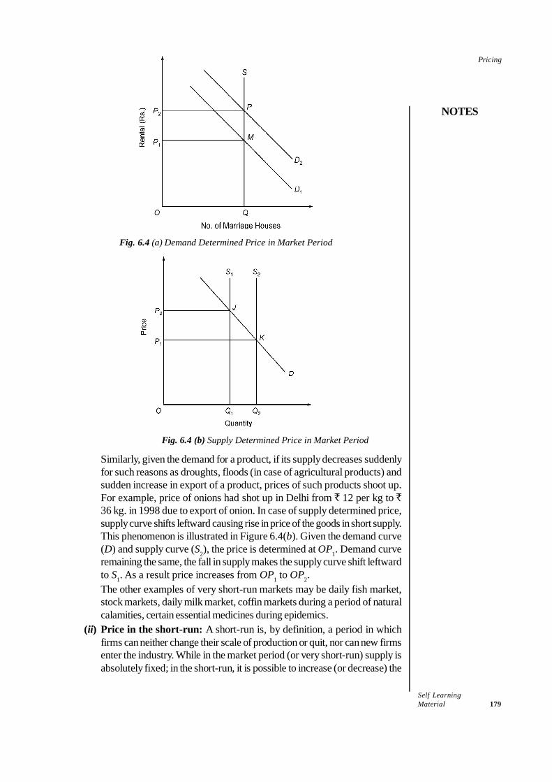
Self LearningMaterial 179
Pricing
NOTES
Fig. 6.4 (a) Demand Determined Price in Market Period
Fig. 6.4 (b) Supply Determined Price in Market Period
Similarly, given the demand for a product, if its supply decreases suddenlyfor such reasons as droughts, floods (in case of agricultural products) andsudden increase in export of a product, prices of such products shoot up.For example, price of onions had shot up in Delhi from ` 12 per kg to `36 kg. in 1998 due to export of onion. In case of supply determined price,supply curve shifts leftward causing rise in price of the goods in short supply.This phenomenon is illustrated in Figure 6.4(b). Given the demand curve(D) and supply curve (S2), the price is determined at OP1. Demand curveremaining the same, the fall in supply makes the supply curve shift leftwardto S1. As a result price increases from OP1 to OP2.The other examples of very short-run markets may be daily fish market,stock markets, daily milk market, coffin markets during a period of naturalcalamities, certain essential medicines during epidemics.
(ii) Price in the short-run: A short-run is, by definition, a period in whichfirms can neither change their scale of production or quit, nor can new firmsenter the industry. While in the market period (or very short-run) supply isabsolutely fixed; in the short-run, it is possible to increase (or decrease) the

Self Learning180 Material
Pricing
NOTES
supply by increasing (or decreasing) the variable inputs. In the short-run,therefore, supply curve is elastic.The determination of market price in the short-run is illustrated in Figure6.5(a) and adjustment of output by the firms to the market price and firm’sequilibrium are shown in Figure 6.5(b). Figure 6.5(a) shows the pricedetermination for the industry by the demand curve DD and supply curveSS, at price OP1 or PQ. This price is fixed for all the firms in the industry.
Fig. 6.5 Pricing under Perfect Competition in the Short-run
Given the price PQ (= OP1), an individual firm can produce and sell anyquantity at this price. But any quantity will not yield maximum profit. Giventheir cost curves, the firms are required to adjust their output to the pricePQ so that they maximize their profit.The process of firm’s output determination and its equilibrium are shown inFigure 6.5(b). Profit is maximum at the level of output where MR = MC.Since price is fixed at PQ, firm’s AR = PQ. If AR is constant, MR = AR.The firm’s MR is shown by AR = MR line. Firm’s upward sloping MC curveintersects AR = MR at point E. At point E, MR = MC. Point E is, therefore,the firm’s equilibrium point. An ordinate drawn from point E to the outputaxis, as shown by the line EM, determines the profit-maxmizing output atOM. At this output the firm’s MR = MC. This satisfies the necessarycondition of maximum profit. The total maximum profit has been shown bythe area P1TNE.The total profit is calculated as Profit = (AR – AC) Q. In Figure 6.5(b), AR= EM; AC = NM; and Q = OM. Substituting these values into the profitequation, we get Profit = (EM – NM) OM. Since EM – NM = EN, Profit =EN × OM = P1TNE. This is the maximum supernormal profit, given theprice and cost curves, in the short run.Firms may make losses in the short-run: While firms may makesupernormal profit, there may be conditions under which firms make lossesin the short-run. For instance, this may happen if market price decreases toP′Q′ due to downward shift in the demand curve from DD to D′D′ [Figure6.5(a)]. This will force a process of output adjustments till firms reach anew equilibrium at point E′. Here again firm’s AR′ = MR′ = MC. But, as

Self LearningMaterial 181
Pricing
NOTES
Figure 6.5(b) shows, AR < AC. Therefore, the firms incur a loss. But, sincein the short-run, it may not be desirable to close down the production, thefirms try to minimize the loss, by adjusting their output downward to OM′where it covers only its MC, i.e., E′M′. The firms survive in the short-runso long as they cover their MC.It is important to note here that in the short-run, a firm in a perfectlycompetitive market may be in a position to earn economic profit. It may aswell be forced to make losses. Once market price for the product isdetermined, it is given for all the firms. No firm is large enough to influencethe prices. If a firm fixes the price of its product lower than the marketprice, it may lose a part of its total profit, or may even incur losses. If itraises the price of its product above the market price, it may not be in aposition to sell its produce in a competitive market. The only option for afirm is to produce as much as it can sell at the given price.
(iii) Pricing in the long-run: In contrast to the short-run conditions, in thelong-run, the firms can adjust their size or quit the industry and new firmscan enter the industry. If market price in the long run is such that AR > AC,then the firms make economic or super normal profit. As a result, new firmsget attracted towards the industry causing increase in market supply at thegiven price. Increase in market supply causes rightward shift in the supplycurve. Similarly, if AR < AC, then firms make losses. Therefore, marginalfirms quit the industry causing decrease in market supply. This causes aleftward shift in the supply curve. The rightward shift in the supply curvepulls down the price and its leftward shift pushes it up. This process continuesuntil price is so determined that AR = AC, and firms earn only normal profit.The price determination in the long-run and output adjustment by individualfirms are illustrated graphically in Figure 6.6(a) and (b).Let us suppose that the long-run demand curve is given by the curve DD′;the short-run supply curve is given by the curve SS1 and price is determinedat OP1. Let us suppose also that all the firms of the industry face identicalLAC and LMC curves as shown in Figure 6.6(b). At market price OP1, allthe firms find their equilibrium at point M in panel (b) of the figure. Atequilibrium point M, OP1 = AR′ = MR′ = LMC. Given the price and cost,firms make an economic profit of MS per unit. The supernormal profit luresother firms into the industry. Consequently, industry’s supply curve shiftsrightward to SS2 causing a fall in price to OP2. At this price, firms are in aposition to cover only LMC (= NQ2) at output OQ2 and are making lossesbecause AR < LAC. Firms incurring losses cannot survive in the long-run.Such firms, therefore, quit the industry. As a result, the total production inthe industry decreases causing a leftward shift in the supply curve, say, tothe position of SS curve. Price is determined at OP0. The existing firmsadjust their output to the new market price OP0 and reach a new equilibriumat point E where equilibrium output is OQ. At the output OQ, firms are in aposition to make only normal profit, since at this output, OP0 = AR = MR =LMC = LAC (= EQ). No firm is in a position to make economic profit, nordoes any firm make losses. Therefore, there is no tendency of new firmsentering the industry or the existing ones going out. At this price and output,individual firms and the industry are both in long-run equilibrium.
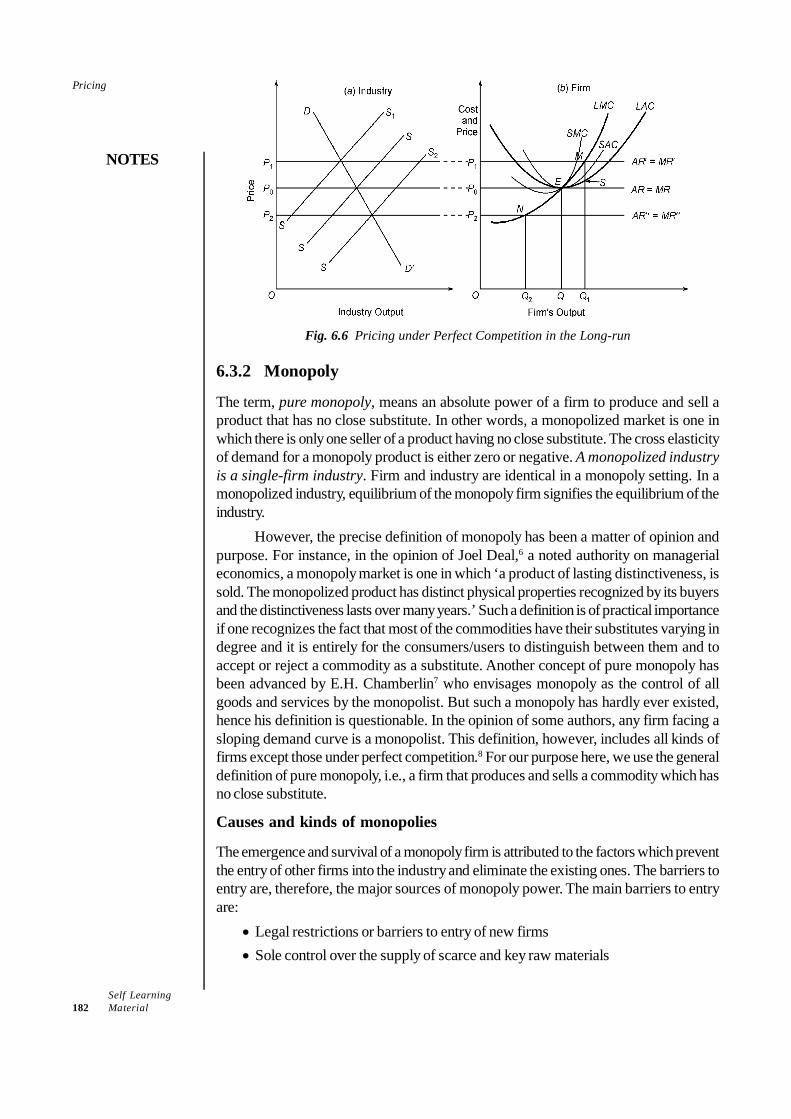
Self Learning182 Material
Pricing
NOTES
Fig. 6.6 Pricing under Perfect Competition in the Long-run
6.3.2 Monopoly
The term, pure monopoly, means an absolute power of a firm to produce and sell aproduct that has no close substitute. In other words, a monopolized market is one inwhich there is only one seller of a product having no close substitute. The cross elasticityof demand for a monopoly product is either zero or negative. A monopolized industryis a single-firm industry. Firm and industry are identical in a monopoly setting. In amonopolized industry, equilibrium of the monopoly firm signifies the equilibrium of theindustry.
However, the precise definition of monopoly has been a matter of opinion andpurpose. For instance, in the opinion of Joel Deal,6 a noted authority on managerialeconomics, a monopoly market is one in which ‘a product of lasting distinctiveness, issold. The monopolized product has distinct physical properties recognized by its buyersand the distinctiveness lasts over many years.’ Such a definition is of practical importanceif one recognizes the fact that most of the commodities have their substitutes varying indegree and it is entirely for the consumers/users to distinguish between them and toaccept or reject a commodity as a substitute. Another concept of pure monopoly hasbeen advanced by E.H. Chamberlin7 who envisages monopoly as the control of allgoods and services by the monopolist. But such a monopoly has hardly ever existed,hence his definition is questionable. In the opinion of some authors, any firm facing asloping demand curve is a monopolist. This definition, however, includes all kinds offirms except those under perfect competition.8 For our purpose here, we use the generaldefinition of pure monopoly, i.e., a firm that produces and sells a commodity which hasno close substitute.
Causes and kinds of monopolies
The emergence and survival of a monopoly firm is attributed to the factors which preventthe entry of other firms into the industry and eliminate the existing ones. The barriers toentry are, therefore, the major sources of monopoly power. The main barriers to entryare:
• Legal restrictions or barriers to entry of new firms• Sole control over the supply of scarce and key raw materials

Self LearningMaterial 183
Pricing
NOTES
• Efficiency in production• Economies of scale
(i) Legal restrictions: Some monopolies are created by law in the public interest.Most of the erstwhile monopolies in the public utility sector in India, e.g., postal, telegraphand telephone services, telecommunication services, generation and distribution ofelectricity, Indian Railways, Indian Airlines and State Roadways, etc., were publicmonopolies. Entry to these industries was prevented by law. Now most of these industriesare being gradually opened too the private sector. Also, the state may create monopoliesin the private sector also, through licence or patent, provided they show the potential ofand opportunity for reducing cost of production to the minimum by enlarging size andinvesting in technological innovations. Such monopolies are known as franchisemonopolies.(ii) Control over key raw materials: Some firms acquire monopoly power becauseof their traditional control over certain scarce and key raw materials which are essentialfor the production of certain goods, e.g., bauxite, graphite, diamond. For instance,Aluminium Company of America had monopolized the aluminium industry before WorldWar II because it had acquired control over almost all sources of bauxite supply9. Suchmonopolies are often called ‘raw material monopolies’. The monopolies of this kindemerge also because of monopoly over certain specific knowledge of technique ofproduction.(iii) Efficiency in production: Efficiency in production, especially under imperfectmarket conditions, may be the result of long experience, innovative ability, financialstrength, availability of market finance at lower cost, low marketing cost, managerialefficiency, etc. Efficiency in production reduces cost of production. As a result, a firm’sgains higher the competitive strength and can eliminate rival firms and gain the status ofa monopoly. Such firms are able to gain governments’ favour and protection.(iv) Economies of scale: The economies of scale are a primary and technical reasonfor the emergence and existence of monopolies in an unregulated market. If a firm’slong-run minimum cost of production or its most efficient scale of production almostcoincides with the size of the market, then the large-size firm finds it profitable in thelong-run to eliminate competition through price cutting in the short-run. Once its monopolyis established, it becomes almost impossible for the new firms to enter the industry andsurvive. Monopolies created on account of this factor are known as natural monopolies.A natural monopoly may emerge out of the technical conditions of efficiency or may becreated by law on efficiency grounds.
Pricing and Output Decision in the Short-run
As under perfect competition, pricing and output decisions under monopoly are based onprofit maximization hypothesis, given the revenue and cost conditions. Although costconditions, i.e., AC and MC curves, in a competitive and monopoly market are generallyidentical, revenue conditions differ. Revenue conditions, i.e., AR and MR curves, aredifferent under monopoly—unlike a competitive firm, a monopoly firm faces a downwardsloping demand curve. The reason is a monopolist has the option and power to reducethe price and sell more or to raise the price and still retain some customers. Therefore,given the price-demand relationship, demand curve under monopoly is a typical downwardsloping demand curve.
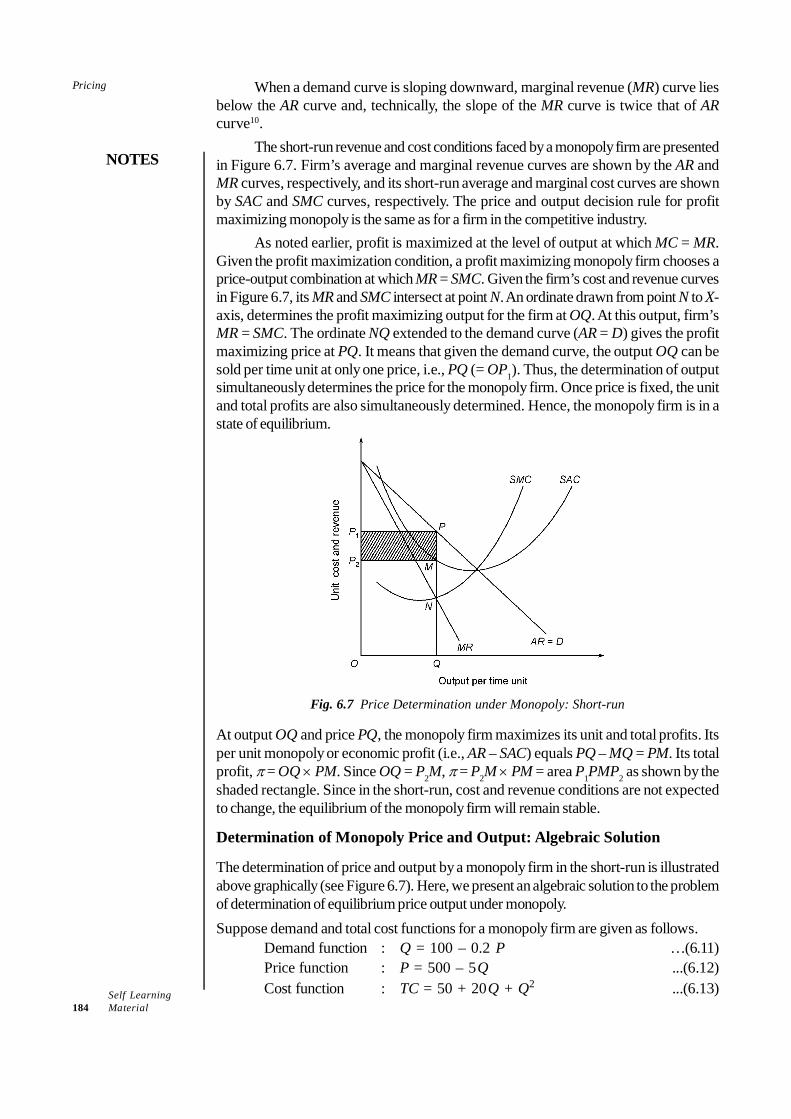
Self Learning184 Material
Pricing
NOTES
When a demand curve is sloping downward, marginal revenue (MR) curve liesbelow the AR curve and, technically, the slope of the MR curve is twice that of ARcurve10.
The short-run revenue and cost conditions faced by a monopoly firm are presentedin Figure 6.7. Firm’s average and marginal revenue curves are shown by the AR andMR curves, respectively, and its short-run average and marginal cost curves are shownby SAC and SMC curves, respectively. The price and output decision rule for profitmaximizing monopoly is the same as for a firm in the competitive industry.
As noted earlier, profit is maximized at the level of output at which MC = MR.Given the profit maximization condition, a profit maximizing monopoly firm chooses aprice-output combination at which MR = SMC. Given the firm’s cost and revenue curvesin Figure 6.7, its MR and SMC intersect at point N. An ordinate drawn from point N to X-axis, determines the profit maximizing output for the firm at OQ. At this output, firm’sMR = SMC. The ordinate NQ extended to the demand curve (AR = D) gives the profitmaximizing price at PQ. It means that given the demand curve, the output OQ can besold per time unit at only one price, i.e., PQ (= OP1). Thus, the determination of outputsimultaneously determines the price for the monopoly firm. Once price is fixed, the unitand total profits are also simultaneously determined. Hence, the monopoly firm is in astate of equilibrium.
Fig. 6.7 Price Determination under Monopoly: Short-run
At output OQ and price PQ, the monopoly firm maximizes its unit and total profits. Itsper unit monopoly or economic profit (i.e., AR – SAC) equals PQ – MQ = PM. Its totalprofit, π = OQ × PM. Since OQ = P2M, π = P2M × PM = area P1PMP2 as shown by theshaded rectangle. Since in the short-run, cost and revenue conditions are not expectedto change, the equilibrium of the monopoly firm will remain stable.
Determination of Monopoly Price and Output: Algebraic Solution
The determination of price and output by a monopoly firm in the short-run is illustratedabove graphically (see Figure 6.7). Here, we present an algebraic solution to the problemof determination of equilibrium price output under monopoly.Suppose demand and total cost functions for a monopoly firm are given as follows.
Demand function : Q = 100 – 0.2 P …(6.11)Price function : P = 500 – 5Q ...(6.12)Cost function : TC = 50 + 20Q + Q2 ...(6.13)
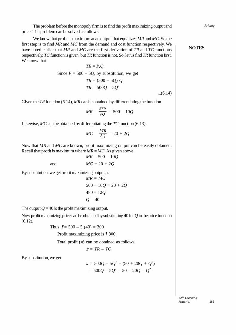
Self LearningMaterial 185
Pricing
NOTES
The problem before the monopoly firm is to find the profit maximizing output andprice. The problem can be solved as follows.
We know that profit is maximum at an output that equalizes MR and MC. So thefirst step is to find MR and MC from the demand and cost function respectively. Wehave noted earlier that MR and MC are the first derivation of TR and TC functionsrespectively. TC function is given, but TR function is not. So, let us find TR function first.We know that
TR = P.QSince P = 500 – 5Q, by substitution, we get
TR = (500 – 5Q) QTR = 500Q – 5Q2
...(6.14)
Given the TR function (6.14), MR can be obtained by differentiating the function.
MR = TRQ
∂∂ = 500 – 10Q
Likewise, MC can be obtained by differentiating the TC function (6.13).
MC = QTR
∂∂ = 20 + 2Q
Now that MR and MC are known, profit maximizing output can be easily obtained.Recall that profit is maximum where MR = MC. As given above,
MR = 500 – 10Qand MC = 20 + 2Q
By substitution, we get profit maximizing output asMR = MC500 – 10Q = 20 + 2Q480 = 12QQ = 40
The output Q = 40 is the profit maximizing output.Now profit maximizing price can be obtained by substituting 40 for Q in the price function(6.12).
Thus, P= 500 – 5 (40) = 300Profit maximizing price is ` 300.
Total profit (p) can be obtained as follows.π = TR – TC
By substitution, we getπ = 500Q – 5Q2 – (50 + 20Q + Q2) = 500Q – 5Q2 – 50 – 20Q – Q2
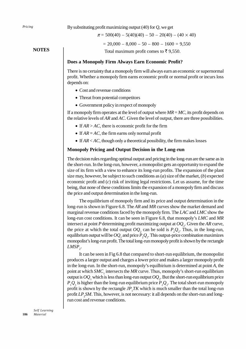
Self Learning186 Material
Pricing
NOTES
By substituting profit maximizing output (40) for Q, we getp = 500(40) – 5(40)(40) – 50 – 20(40) – (40 ¥ 40)
= 20,000 – 8,000 – 50 – 800 – 1600 = 9,550Total maximum profit comes to ` 9,550.
Does a Monopoly Firm Always Earn Economic Profit?
There is no certainty that a monopoly firm will always earn an economic or supernormalprofit. Whether a monopoly firm earns economic profit or normal profit or incurs lossdepends on:
• Cost and revenue conditions• Threat from potential competitors• Government policy in respect of monopoly
If a monopoly firm operates at the level of output where MR = MC, its profit depends onthe relative levels of AR and AC. Given the level of output, there are three possibilities.
• If AR > AC, there is economic profit for the firm• If AR = AC, the firm earns only normal profit• If AR < AC, though only a theoretical possibility, the firm makes losses
Monopoly Pricing and Output Decision in the Long-run
The decision rules regarding optimal output and pricing in the long-run are the same as inthe short-run. In the long-run, however, a monopolist gets an opportunity to expand thesize of its firm with a view to enhance its long-run profits. The expansion of the plantsize may, however, be subject to such conditions as (a) size of the market, (b) expectedeconomic profit and (c) risk of inviting legal restrictions. Let us assume, for the timebeing, that none of these conditions limits the expansion of a monopoly firm and discussthe price and output determination in the long-run.
The equilibrium of monopoly firm and its price and output determination in thelong-run is shown in Figure 6.8. The AR and MR curves show the market demand andmarginal revenue conditions faced by the monopoly firm. The LAC and LMC show thelong-run cost conditions. It can be seen in Figure 6.8, that monopoly’s LMC and MRintersect at point P determining profit maximizing output at OQ2. Given the AR curve,the price at which the total output OQ2 can be sold is P2Q2. Thus, in the long-run,equilibrium output will be OQ2 and price P2Q2. This output-price combination maximizesmonopolist’s long-run profit. The total long-run monopoly profit is shown by the rectangleLMSP2.
It can be seen in Fig 6.8 that compared to short-run equilibrium, the monopolistproduces a larger output and charges a lower price and makes a larger monopoly profitin the long-run. In the short-run, monopoly’s equilbirium is determined at point A, thepoint at which SMC1 intersects the MR curve. Thus, monopoly’s short-run equilibriumoutput is OQ1 which is less than long-run output OQ2. But the short-run equilibrium priceP1Q1 is higher than the long-run equilibrium price P2Q2. The total short-run monopolyprofit is shown by the rectangle JP1TK which is much smaller than the total long-runprofit LP2SM. This, however, is not necessary: it all depends on the short-run and long-run cost and revenue conditions.
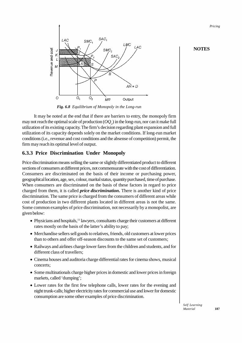
Self LearningMaterial 187
Pricing
NOTES
Fig. 6.8 Equilibrium of Monopoly in the Long-run
It may be noted at the end that if there are barriers to entry, the monopoly firmmay not reach the optimal scale of production (OQ2) in the long-run, nor can it make fullutilization of its existing capacity. The firm’s decision regarding plant expansion and fullutilization of its capacity depends solely on the market conditions. If long-run marketconditions (i.e., revenue and cost conditions and the absense of competition) permit, thefirm may reach its optimal level of output.
6.3.3 Price Discrimination Under Monopoly
Price discrimination means selling the same or slightly differentiated product to differentsections of consumers at different prices, not commensurate with the cost of differentiation.Consumers are discriminated on the basis of their income or purchasing power,geographical location, age, sex, colour, marital status, quantity purchased, time of purchase.When consumers are discriminated on the basis of these factors in regard to pricecharged from them, it is called price discrimination. There is another kind of pricediscrimination. The same price is charged from the consumers of different areas whilecost of production in two different plants located in different areas is not the same.Some common examples of price discrimination, not necessarily by a monopolist, aregiven below:
• Physicians and hospitals,11 lawyers, consultants charge their customers at differentrates mostly on the basis of the latter’s ability to pay;
• Merchandise sellers sell goods to relatives, friends, old customers at lower pricesthan to others and offer off-season discounts to the same set of customers;
• Railways and airlines charge lower fares from the children and students, and fordifferent class of travellers;
• Cinema houses and auditoria charge differential rates for cinema shows, musicalconcerts;
• Some multinationals charge higher prices in domestic and lower prices in foreignmarkets, called ‘dumping’;
• Lower rates for the first few telephone calls, lower rates for the evening andnight trunk-calls; higher electricity rates for commercial use and lower for domesticconsumption are some other examples of price discrimination.

Self Learning188 Material
Pricing
NOTES
Necessary Conditions
First, different markets must be separable for a seller to be able to practicediscriminatory pricing. The markets for different classes of consumers must be soseparated that buyers of one market are not in a position to resell the commodity in theother. Markets are separated by (i) geographical distance involving high cost oftransportation, i.e., domestic versus foreign markets; (ii) exclusive use of the commodity,e.g., doctor’s services; (iii) lack of distribution channels, e.g., transfer of electricity fromdomestic use (lower rate) to industrial use (higher rate).Second, the elasticity of demand for the product must be different in differentmarkets. The purpose of price discrimination is to maximize the profit by exploiting themarkets with different price elasticities. It is the difference in the elasticity which providesmonopoly firm with an opportunity for price discrimination. If price elasticities of demandin different markets are the same, price discrimination would reduce the profit by reducingdemand in the high price markets.Third, there should be imperfect competition in the market. The firm must havemonopoly over the supply of the product to be able to discriminate between differentclasses of consumers, and charge different prices.Fourth, profit maximizing output must be much larger than the quantity demanded in asingle market or by a section of consumers.
6.3.4 Price Discrimination by Degrees
The degree of price discrimination refers to the extent to which a seller can divide themarket or the consumers and can take advantage of it in extracting the consumer’ssurplus. The economic literature presents three degrees of price discrimination.First degree12: The first degree price discrimination is the limit of discriminatorypricing. First degree or perfect price discrimination is feasible when the market size ofthe product is small and the monopolist is in a position to know the price each consumeror each group of consumers is willing to pay, (i.e., he knows his buyer’s demand curvefor his product), then he sets the price accordingly and tries to extract the entire consumersurplus.13 What the seller does is that he sets the price at its highest level—the level atwhich all those who are willing to buy the commodity buy at least one unit each. Afterextracting the consumer surplus of this segment of consumers for the first unit ofcommodity, the monopolist gradually lowers down the price, so that the consumer surplusof the users of the second unit is extracted. This procedure is continued until the entireconsumers’ surplus available at the equilibrium price, i.e., at the price at which MC =MR, is extracted. Consider, for example, the case of medical services of exclusive use.A doctor who knows or can guess the paying capacity of his patients can charge thehighest possible fee from presumably the richest patient and the lowest fee from thepoorest patient.Second degree: Where market size is very large, perfect discrimination is neitherfeasible nor desirable. In that case, a monopolist uses second degree discrimination orthe ‘block pricing method’. A monopolist adopting the second degree price discriminationintends to siphon off only the major part of the consumer’s surplus, rather than the wholeof it. The monopolist divides the potential buyers into blocks, e.g., rich, middle class andpoor, and sells the commodity in blocks. The monopolist sells its product first to the richcustomers at the highest possible price. Once this part of the market is supplied, the firmlowers down the price for middle class buyers. Finally, bottom price is used for the poorclass of buyers.

Self LearningMaterial 189
Pricing
NOTES
The second degree price discrimination is feasible where (i) the number ofconsumers is large and price rationing can be done, as in case of utility services liketelephones, supply of water, etc.; (ii) demand curve for all the consumers is identical;(iii) a single rate is applicable for a large number of buyers. As shown in Figure 6.9, amonopolist practicing second degree price discrimination, charges the highest price OP1for OQ1 units and a lower price OP2 for the next Q1Q2 units, and the lowest price OP3for the next Q2Q3 units. Thus, by adopting a block pricing system, the monopolist maximizeshis total revenue (TR) at
TR = (OQ1 . AQ1) + (Q1Q2 . BQ2) + (Q2Q3 . CQ3)
Third degree: When a profit maximizing monopolist sets different prices in differentmarkets having demand curves with different elasticities, he is practising the third degreeprice discrimination. It happens quite often that a monopolist has to sell his goods intwo or more markets, completely separated from one another, each having a demandcurve with different elasticity. A uniform price cannot be set for all the markets withoutlosing profits. The monopolist is, therefore, required to find different price-quantitycombinations that can maximize his profit in each market. For this purpose, he divideshis total output between the market segments so that his MC = MR in each market, andfixes price accordingly.
Fig. 6.9 Second Degree Price Discrimination
For example, suppose that a monopolist has only two markets, A and B. The demandcurve (Da) and marginal revenue curve (MRa) given in Figure 6.10(a), represent the ARand MR curves in market A. Db and MRb in Figure 6.10(b) represent the AR and MRcurves in market B. The horizontal summation of Da and Db gives the total demandcurve for the two markets, a shown by AR = D in Figure 6.10(c) and the horizontalsummation of MRa and MRb gives the aggregated MR [(Figure 6.10(c)]. The firm’smarginal cost is shown by MC that intersects MR at point T. Thus, the optimum level ofoutput for the firm is determined at OQ at which MR = MC.
Fig. 6.10 Third Degree Price Discrimination
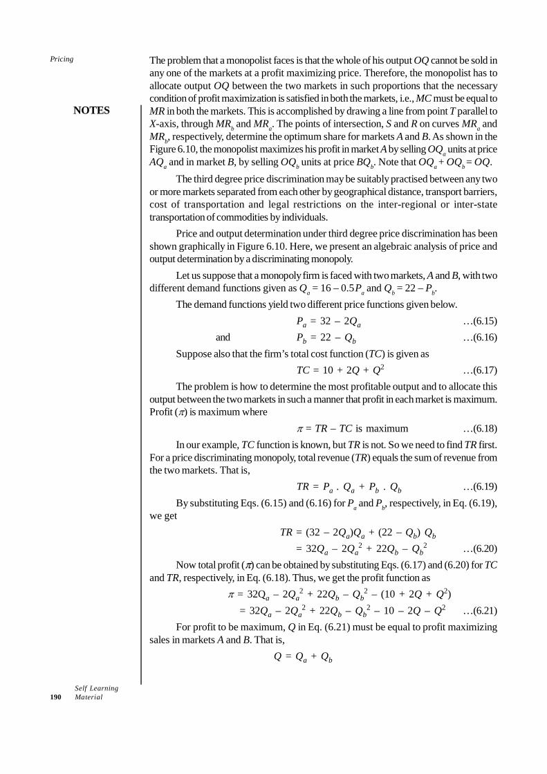
Self Learning190 Material
Pricing
NOTES
The problem that a monopolist faces is that the whole of his output OQ cannot be sold inany one of the markets at a profit maximizing price. Therefore, the monopolist has toallocate output OQ between the two markets in such proportions that the necessarycondition of profit maximization is satisfied in both the markets, i.e., MC must be equal toMR in both the markets. This is accomplished by drawing a line from point T parallel toX-axis, through MRb and MRa. The points of intersection, S and R on curves MRa andMRb, respectively, determine the optimum share for markets A and B. As shown in theFigure 6.10, the monopolist maximizes his profit in market A by selling OQa units at priceAQa and in market B, by selling OQb units at price BQb. Note that OQa + OQb = OQ.
The third degree price discrimination may be suitably practised between any twoor more markets separated from each other by geographical distance, transport barriers,cost of transportation and legal restrictions on the inter-regional or inter-statetransportation of commodities by individuals.
Price and output determination under third degree price discrimination has beenshown graphically in Figure 6.10. Here, we present an algebraic analysis of price andoutput determination by a discriminating monopoly.
Let us suppose that a monopoly firm is faced with two markets, A and B, with twodifferent demand functions given as Qa = 16 – 0.5Pa and Qb = 22 – Pb.
The demand functions yield two different price functions given below.Pa = 32 – 2Qa …(6.15)
and Pb = 22 – Qb …(6.16)Suppose also that the firm’s total cost function (TC) is given as
TC = 10 + 2Q + Q2 …(6.17)The problem is how to determine the most profitable output and to allocate this
output between the two markets in such a manner that profit in each market is maximum.Profit (π) is maximum where
π = TR – TC is maximum …(6.18)In our example, TC function is known, but TR is not. So we need to find TR first.
For a price discriminating monopoly, total revenue (TR) equals the sum of revenue fromthe two markets. That is,
TR = Pa . Qa + Pb . Qb …(6.19)By substituting Eqs. (6.15) and (6.16) for Pa and Pb, respectively, in Eq. (6.19),
we getTR = (32 – 2Qa)Qa + (22 – Qb) Qb
= 32Qa – 2Qa2 + 22Qb – Qb
2 …(6.20)Now total profit (p) can be obtained by substituting Eqs. (6.17) and (6.20) for TC
and TR, respectively, in Eq. (6.18). Thus, we get the profit function as π = 32Qa – 2Qa
2 + 22Qb – Qb2 – (10 + 2Q + Q2)
= 32Qa – 2Qa2 + 22Qb – Qb
2 – 10 – 2Q – Q2 …(6.21)For profit to be maximum, Q in Eq. (6.21) must be equal to profit maximizing
sales in markets A and B. That is, Q = Qa + Qb
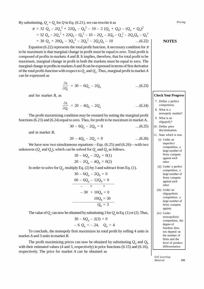
Self LearningMaterial 191
Pricing
NOTES
By substituting, Qa + Qb for Q in Eq. (6.21), we can rewrite it asp = 32 Qa – 2Qa
2 + 22Qb – Qb2 – 10 – 2 (Qa + Qb) – (Qa + Qb)
2
= 32 Qa – 2Qa2 + 22Qb – Qb
2 – 10 – 2Qa – 2Qb – Qa2 – 2QaQb – Qb
2
= 30 Qa + 20Qb – 3Qa2 – 2Qb
2 – 2QaQb – 10 …(6.22)Equation (6.22) represents the total profit function. A necessary condition for p
to be maximum is that marginal change in profit must be equal to zero. Total profit iscomposed of profits in markets A and B. It implies, therefore, that for total profit to bemaximum, marginal change in profit in both the markets must be equal to zero. Themarginal change in profits in markets A and B can be expressed in terms of first derivativeof the total profit-function with respect to Qa and Qb. Thus, marginal profit in market Acan be expressed as
aQ∂π
∂ = 30 – 6Qa – 2Qb …(6.23)
and for market B, as
bQ∂π
∂ = 20 – 4Qb – 2Qa …(6.24)
The profit maximizing condition may be restated by setting the marginal profitfunctions (6.23) and (6.24) equal to zero. Thus, for profit to be maximum in market A,
30 – 6Qa – 2Qb = 0 …(6.25)and in market B,
20 – 4Qb – 2Qa = 0 …(6.26)We have now two simultaneous equations—Eqs. (6.25) and (6.26)—with two
unknowns (Qa and Qb), which can be solved for Qa and Qb as follows.30 – 6Qa – 2Qb = 0(1)20 – 2Qa – 4Qb = 0(2)
In order to solve for Qb, multiply Eq. (2) by 3 and subtract from Eq. (1).30 – 6Qa – 2Qb = 060 – 6Qa – 12Qb = 0
– + +– 30 + 10Qb = 0
10Qb = 30 Qb = 3
The value of Qa can now be obtained by substituting 3 for Qb in Eq. (1) or (2). Thus,30 – 6Qa – 2(3) = 0– 6 Qa = – 24, Qa = 4
To conclude, the monopoly firm maximizes its total profit by selling 4 units inmarket A and 3 units in market B.
The profit maximizing prices can now be obtained by substituting Qa and Qbwith their estimated values (4 and 3, respectively) in price functions (6.15) and (6.16),respectively. The price for market A can be obtained as
Check Your Progress
7. Define a perfectcompetition.
8. What is amonopoly market?
9. What is anoligopoly?
10. Define pricediscrimination.
11. State which is true(i) Under an
imperfectcompetition, alarge number offirms competeagainst eachother
(ii) Under a perfectcompetition, alarge number offirms competeagainst eachother
(iii) Under anoligopolisticcompetition, alarge number offirms competeagainst
(iv) Undermonopolisticcompetition, thedegree offreedom doesnot depend onthe number offirms and thelevel of productdifferentiation
Self Learning192 Material
Pricing
NOTES
Pa = 32 – 2 Qa = 32 – 2 (4) = 24and price for market B as
Pb = 22 – Qb = 22 – 3 = 19Thus, in market A, price = ̀ 24 and in market B, price = ̀ 19.
Now that prices and sales for the two markets are known, total profit can beobtained by substituting numerical values for Qa and Qb in profit function (6.22). Theprofit function (6.23) is reproduced below.
π = 30 Qa + 20 Qb – 3Qa2 – 2Qb
2 – 2QaQb – 10By substituting 4 for Qa and 3 for Qb, we get
p = 30 (4) + 20(3) – 3(4)(4) – 2 (3)(3) – 2(4)(3) – 10 = 120 + 60 – 48 – 18 – 24 –10 = 80
The total profit is ̀ 80. This profit satisfies the conditions of the maximum profit.It is, therefore, maximum.
6.4 PRODUCT LINE PRICING
The price theory or microeconomic models of price determination are based on theassumption that a firm produces a single, homogeneous product. In actual practice,however, production of a single homogeneous product by a firm is an exception ratherthan a rule. Almost all firms have more than one product in their line of production. Eventhe most specialized firms produce a commodity in multiple models, styles and sizes,each so much differentiated from the other that every model or size of the product maybe considered a different product. For example, the various models of refrigerators, TVsets, cell phones, computers and car models produced by the same company may betreated as different products for at least pricing purpose. The various models are sodifferentiated that consumers view them as different products14 and, in some cases, asclose substitutes for each other. It is, therefore, not surprising that each model or producthas different AR and MR curves and that one product of the firm competes against theother product. The pricing under these conditions is known as multi-product pricing orproduct-line pricing.
The major problem in pricing multiple products is that each product has a separatedemand curve. But, since all the products are produced under one establishment byinterchangeable production facilities, they have only one joint and one inseparable marginalcost curve. That is, while revenue curves, AR and MR, are separate for each product,cost curves, AC and MC, are inseparable. Therefore, the marginal rule of pricing cannotbe applied straightaway to fix the price of each product separately. The problem, however,has been provided with a solution by E.W. Clemens.15 The solution is similar to thetechnique employed to illustrate third degree price discrimination under profit maximizationassumption. As a discriminating monopoly tries to maximize its revenue in all its markets,so does a multi-product firm in respect of each of its products.
To illustrate product line pricing, let us suppose that a firm has four differentproducts—A, B, C and D in its line of production. The AR and MR curves for the fourbranded products are shown in four segments of Figure 6.11. The marginal cost for allthe products taken together is shown by the curve MC, which is the factory marginalcost curve. Let us suppose that when the MRs for the individual products are horizontallysummed up, the aggregate MR (not given in the figure) passes through point C on the
Check Your Progress
12. The degree of pricediscriminationrefers to:(i) The demand for
the industry as awhole; the sumof the quantitydemanded byeach individualconsumer or userat differentprices
(ii) A period inwhich firms canneither changetheir scale ofproduction norquit, nor cannew firms enterthe industry
(iii) The extent towhich a sellercan divide themarket or theconsumers andcan takeadvantage of it inextracting theconsumer'ssurplus
(iv) The decisionrules regardingoptimal outputand pricing inthe long-run

Self LearningMaterial 193
Pricing
NOTES
MC curve. If a line parallel to the X-axis, is drawn from point C to the Y-axis through theMRs, the intersecting points will show the points where MC and MRs are equal for eachproduct, as shown by the line EMR, the Equal Marginal Revenue line. The points ofintersection between EMR and MRs determine the output level and price for each product.The output of the four products are given as OQa of product A; QaQb of B; QbQc of C;and QcQd of D. The respective prices for the four products are: PaQa for product A;PbQb for B; PcQc for C, and PdQd for D. These price and output combinations maximizethe profit from each product and hence the overall profit of the firm.
Fig. 6.11 Product Line Pricing
6.4.1 Joint Product Pricing
Joint products are two or more products manufactured from the same process or operationby the firm. The firm has to choose prices for joint products. It is a more complexprocess to price joint products as compared to pricing a single product. The characteristicsof each product are different. There are two demand curves. Demand for one productcould be greater than the other. Consumers of one product could be more price elastic thanconsumers of the other. Hence, consumers will be more sensitive to changes in the priceof the product. Since both products, have been produced jointly, they share a commonmarginal cost curve. Complexities are also noticed in the production function. Since theyare bi-products or produced from the same inputs, also known as substitutes in production,the production of both the products could be linked. The production of the joint productcould be in fixed proportions or in variable proportions as well.
6.5 SUMMARY
• Economist’s concept of profit is of ‘pure profit’, also called ‘economic profit’ or‘just profit’. Pure profit is a return over and above the opportunity cost, i.e., theincome which a businessman might expect from the second best alternative useof his resources.
• In accounting sense, profit is surplus of total revenue over and above all paid-outcosts, including both manufacturing and overhead expenses.
• The concept of ‘economic profit’ differs from ‘accounting profit’. Economic profitalso takes into account the implicit or imputed costs.
Check Your Progress
13. Define product-linepricing or multi-product pricing.
14. What is the majorproblem faced inpricing multipleproducts?

Self Learning194 Material
Pricing
NOTES
• Accounting profit does not take into account the opportunity cost but economicprofit does.
• Pure profit may thus be defined as ‘a residual left after all contractual costs havebeen met, including the transfer costs of management, insurable risks, depreciationand payments to shareholders sufficient to maintain investment at its currentlevel’.
• The conventional economic theory assumes profit maximization as the onlyobjective of business firms.
• Baumols’s theory of sales maximization is one of the most important alternativetheories of firm’s behaviour. The basic premise of Baumol’s theory is that salesmaximization, rather than profit maximization, is the plausible goal of the businessfirms.
• He argues that, in modern business, management is separated from ownership,and managers enjoy the discretion to pursue goals other than profit maximization.
• Perfect competition is a market setting in which there is a large number of sellersof a homogeneous product. Each seller supplies a very small fraction of the totalsupply.
• A monopolized market is one in which there is only one seller of a product havingno close substitute. A monopolized industry is a single-firm industry.
• The main barriers to entry in a monopoly market are:o Legal restrictions or barriers to entry of new firmso Sole control over the supply of scarce and key raw materialso Efficiency in production, ando Economies of scale
• As under perfect competition, pricing and output decisions under monopoly arebased on profit maximization hypothesis, given the revenue and cost conditions.Although cost conditions, i.e., AC and MC curves, in a competitive and monopolymarket are generally identical, revenue conditions differ.
• There is no certainty that a monopoly firm will always earn an economic orsupernormal profit.
• Price discrimination means selling the same or slightly differentiated product todifferent sections of consumers at different prices, not commensurate with thecost of differentiation.
• The degree of price discrimination refers to the extent to which a seller can dividethe market or the consumers and can take advantage of it in extracting theconsumer’s surplus.
• The economic literature presents three degrees of price discrimination— firstdegree, second and third degree.
• The various models developed by firms are so differentiated that consumers viewthem as different products and, in some cases, as close substitutes for each other.One product of the firm competes against the other product. The pricing underthese conditions is known as multi-product pricing or product-line pricing.
• The major problem in pricing multiple products is that each product has a separatedemand curve.

Self LearningMaterial 195
Pricing
NOTES
6.6 KEY TERMS
• Profit: In accounting sense, profit is surplus of total revenue over and above allpaid-out costs, including both manufacturing and overhead expenses.
• Pure profit: Pure profit may be defined as ‘a residual left after all contractualcosts have been met, including the transfer costs of management, insurable risks,depreciation and payments to shareholders sufficient to maintain investment at itscurrent level’.
• Perfect competition: Perfect competition is a market setting in which there is alarge number of sellers of a homogeneous product.
• Monopoly: A monopoly market is one in which there is only one seller of aproduct having no close substitute.
• Price discrimination: Price discrimination means selling the same or slightlydifferentiated product to different sections of consumers at different prices, notcommensurate with the cost of differentiation.
• Product-line pricing: The various models of any one product developed byfirms are so differentiated that consumers view them as different products and, insome cases, as close substitutes for each other; one product of the firm competesagainst the other product. The pricing under these conditions is known as multi-product pricing or product-line pricing.
6.7 ANSWERS TO ‘CHECK YOUR PROGRESS’
1. Pure profit may be defined as a residual left after all contractual costs have beenmet, including the transfer costs of management, insurable risks, depreciation andpayments to shareholders sufficient to maintain investment at its current level.
2. The conventional economic theory assumes profit maximization as the onlyobjective of business firms.
3. The basic premise of Baumol’s theory is that sales maximization, rather thanprofit maximization, is the plausible goal of the business firms.
4. The two basic models developed by Baumol are: (i) Static model and (ii) Dynamicmodel–each with and without advertising.
5. (ii) Takes into account the implicit or imputed costs6. (ii) Most managers seek to maximize sales revenue rather than profits7. Perfect competition is a market setting in which there are large number of sellers
of a homogeneous product. Each seller supplies a very small fraction of the totalsupply.
8. A monopoly market is one in which there is only one seller of a product having noclose substitute. In a monopolized market structure, the industry is a single-firm-industry.
9. The control over the pricing discretion increases under oligopoly where degree ofcompetition is quite low, lower than that under monopolistic competition. Thefirms have a good deal of control over the price of their products and can exercisetheir discretion in pricing decisions, especially where product differentiation isprominent.

Self Learning196 Material
Pricing
NOTES
10. Price discrimination means selling the same or slightly differentiated product todifferent sections of consumers at different prices, not commensurate with thecost of differentiation.
11. (ii) Under a perfect competition, a large number of firms compete against eachother
12. (iii) The extent to which a seller can divide the market or the consumers and cantake advantage of it in extracting the consumer's surplus
13. Although it is said that a firm produces only one product, the general practice,however, is to produce a commodity in multiple models, styles and sizes. Thevarious models are so differentiated that consumers view them as differentproducts14 and, in some cases, as close substitutes for each other. The pricingunder these conditions is known as multi-product pricing or product-line pricing.
14. The major problem in pricing multiple products is that each product has a separatedemand curve.
6.8 QUESTIONS AND EXERCISES
Short-Answer Questions
1. Distinguish between accounting profit and economic profit.2. What are the two theoretical conditions for profit maximization?3. Why do business managers pursue the goals of sales maximization according to
Baumol?4. Distinguish between a franchise monopoly and natural monopolies.5. What are the major barriers in entering a monopolized market?6. What are the necessary conditions of price discrimination?
Long-Answer Questions
1. Critically analyse Baumol’s theory of sales maximization.2. Discuss the characteristics of a perfectly competitive market. Explain and illustrate
how price is determined under perfect competition in both short and long-run.3. Explain and illustrate how price and output are determined under monopoly both
in the short and long-run.4. Discuss the three degrees of price discrimination with the help of illustrations.5. Illustrate product-line pricing.
6.9 FURTHER READING/ENDNOTES
Varshney and Maheshwari. 2011. Managerial Economics. New Delhi: Sultan Chandand Sons.
Mankar, V. G. 1982. Business Economics. New Delhi: Himalya Publishing House.Dufty, N.F. 1966. Managerial Economics. New York: Asia Publishing House.
Self LearningMaterial 197
Pricing
NOTES
Endnotes
1. Dean, Joel, Managerial Economics, (Asia Publishing House, Bombay), 1960, p. 3.2. For example, Indian Income Tax Act makes only partial allowance for expenses on
‘entertainment and advertisement’.3. Baumol, W.J. Business Behaviour, Value and Growth (New York, Macmillan, 1959,
Revised edition, Harcourt Brace and World Inc., 1967).4. As summarized Baumol’s Economic Theory and Operations Analysis, 4th Edn.5. The equilibrium is associated with output OQ3 and profit TQ3.6. Managerial Economics, (Prentice-Hall, Englewood Cliffs, N.J.), 1951.7. The Theory of Monopolistic Competition, (Harvard University Press, Mass, 1933).8. Watson, D.S., Price Theory and its Uses, (Scientific Book Agency, Calcutta, 1967),
p. 294.9. Ferguson, C.E., Macroeconomic Theory, (Richard D. Irwin, Illinois, 1972), p. 28.
10. Proof. Let us suppose a linear demand function is given as Q = ∝ – βp. From thisdemand function, a price function is derived as P = a – bQ, where b gives slope ofthe demand curve.Given the price function, total revenue equation can be worked out as
TR = Q. P = Q (a – bQ) = aQ – bQ2
Since MR equals the first derivative of the TR equation,
TRQ
∂∂
= a – 2 bQ
Obviously, the slope of MR curve is – 2b whereas the slope of AR = – b. Thus therate of fall in MR is twice that of AR.
11. A study of medical doctors in the US by Ruben A. Kessel, “Price Discrimination inMedicine,” JL of Law and Eco., October 1959, reveals that charity, not profitmaximization, is the objective of price discrimination. The idea behind charging ahigher fee from the rich patients is to finance the treatment of poor. This is howevera rare phenomenon. One can find such medical practioners and hospitals in Indiaalso.
12. Joan Robinson calls it ‘perfect discrimination’ from a monopolist’s point of view.13. Consumer surplus is the difference between the price a consumer is willing to pay
and the price he actually pays.14. For Example, the different models of Maruti cars, viz., Maruti 800, Zen, Maruti
1000, Esteem, Maruti Van and Wagon-R, etc.15. Clemens, E.W., ‘Price Discrimination and Multiple Product Firm’, Review of
Economic Studies (1950–51). Reprinted in Industrial Organisation and Public policy,Am. Eco. Assn. (Richard D. Irwin, Illinois, 1959).

Self LearningMaterial 199
Profit Management
NOTES
UNIT 7 PROFIT MANAGEMENT
Structure7.0 Introduction7.1 Unit Objectives7.2 Concept of Profit Management
7.2.1 Monopoly Power as Source of Profit7.2.2 Problems in Profit Measurement7.2.3 Problem in Measuring Depreciation7.2.4 Treatment of Capital Gains and Losses7.2.5 Current vs Historical Costs
7.3 Profit Planning and Control7.3.1 Profit as Control Measure
7.4 Summary7.5 Key Terms7.6 Answers to ‘Check Your Progress’7.7 Questions and Exercises7.8 Further Reading/Endnotes
7.0 INTRODUCTION
The question that arises from business analysis point of view is ‘what is the most commonobjective of business firms?’ There is no definite answer to this question. Perhaps thebest way to find out the common objective of business firms is to ask the businessowners and managers themselves. However, Baumol has remarked that firms and theirexecutives are often not clear about the objectives they pursue. As discussed earlier inthe previous unit, profit maximization is regarded as the most common and theoreticallymost plausible objective of business firms. Objectives of business firms can be various.There is no unanimity among economists and researchers on the objectives of businessfirms. One thing is, however, certain that the survival of a firm depends on the profit itcan make. In this unit, we will discuss theory of profit and problems in measuring profit.
7.1 UNIT OBJECTIVES
After going through this unit, you will be able to:• Understand the concept of profit management and discuss its problems• Explain the measures of profit planning and control
7.2 CONCEPT OF PROFIT MANAGEMENT
What are the sources of profit? Economists are not unanimous on this issue. It is in, fact,this question that has been a source of an unsettled controversy and has led to theemergence of various theories of profit. In this section, we discuss briefly the maintheories of profit.
1. Walker’s Theory of Profit: Profit as Rent of AbilityOne of the most widely known theories of profit was propounded by American economistF.A. Walker. According to him, profit is the rent of ‘exceptional abilities that an

Self Learning200 Material
Profit Management
NOTES
entrepreneur may possess’ over others. Just as land rent is the difference between theyields of the least and the most fertile lands, profit is the difference between the earningsof the least and the most efficient entrepreneurs. In formulating his profit theory, Walkerassumed a state of perfect competition in which all firms are presumed to possess equalmanagerial ability. Each firm would receive only the wages of management which, inWalker’s view, form no part of pure profit. He regarded wages of management asordinary wages. Thus, under perfectly competitive conditions, there would be no pureprofit and all firms would earn only managerial wages, which is popularly known as‘normal profit’.
2. Clark’s Dynamic Theory of Profit
According to neoclassical economist J. B. Clark,1 profits arise in a dynamic economy,not in a static one. A static economy is one in which things do not change significantly;population and capital are stationary; production process remains unchanged over time;goods continue to remain homogeneous; factors enjoy freedom of mobility but do notmove because their marginal product in every industry is the same; there is no uncertaintyand hence no risk; and if there is any risk, it is insurable. In a static economy, therefore,all firms make only the ‘normal profit’, i.e., the wages of management.
On the other hand, a dynamic economy is characterized by the following genericchanges: (i) increase in population, (ii) increase in capital, (iii) improvement inproduction technique, (iv) changes in the forms of business organization, and(v) increase in and multiplication of consumer wants. The major functions ofentrepreneurs or managers in a dynamic world are to take advantage of the genericchanges and promote their business, expand their sales and reduce their costs. Theentrepreneurs who successfully take advantage of changing conditions in a dynamiceconomy make pure profit, i.e., profit in addition to ‘normal profit’.
Pure profits, however, exist only in the short run. In the long run, competitionforces other firms to imitate the changes made by the leading firms. This leads to a risein demand for factors of production and, therefore, rise in factor prices and rise in costof production. On the other hand, rise in output causes a decline in product prices, giventhe demand. The ultimate result is that pure profit disappears. In Clark’s own words,‘profit is an elusive sum which entrepreneurs grasp but cannot hold. It slips through theirfingers and bestows itself on all members of the society’.
This, however, should not mean that profits arise in a dynamic economy only fora short period and disappear for ever. In fact, in a dynamic economy, generic changestake place continuously and managers with foresight continue to take advantage of thechanges and make profit in excess of normal profit. According to Clark, emergence,disappearance and re-emergence of profit is a continuous process.
3. Hawley’s Risk Theory of Profit
The risk theory of profit was propounded by American economist F. B. Hawley in 1893.Risk in business may arise for such reasons as obsolescence of a product, sudden fall inprices, non-availability of certain crucial materials, introduction of a better substitute bya competitor, and risks due to fire. Hawley regarded risk-taking as an inevitableaccompaniment of dynamic production and those who take risks have a sound claim toan additional reward, known as ‘profit’. According to Hawley, profit is simply the pricepaid by society for assuming business risks. In his opinion, businessmen would not assumerisk without expecting adequate compensation in excess of actuarial value, i.e., thepremium on calculable risk. They would always look for a return in excess of the wages

Self LearningMaterial 201
Profit Management
NOTES
of management for bearing risk. The reason why Hawley maintained that profit asreward over and above the actuarial risk is that the assumption of risk is irksome; it givesrise to trouble, anxiety and disutilities of various kinds. Therefore, assuming risk givesthe entrepreneur a claim to a reward in excess of actuarial value of risk. Profit, accordingto Hawley, consists of two parts: one part represents compensation for actuarial oraverage loss incidental to the various classes of risks necessarily assumed by theentrepreneur; and the remaining part represents an inducement to suffer the consequencesof being exposed to risk in their entrepreneurial adventures.
Hawley believed that profits arise from factor ownership only so long as ownershipinvolves risk. According to him, an entrepreneur has to assume risk to qualify for profit.If an entrepreneur avoids risk by insuring against it, he would cease to be an entrepreneurand would not receive any profit. In his opinion, it is the uninsured risks out of whichprofits arise, and until the uncertainty ends with the sale of entrepreneur’s products, theamount of reward cannot be determined. Profit, in his opinion is a residue. Hawley’stheory is, thus, a residual theory of profit.
4. Knight’s Theory of ProfitAmerican economist Frank H. Knight2 treated profit as a residual return to uncertaintybearing, not to risk bearing. Obviously, Knight made a distinction between risk anduncertainty. He divided risk into calculable and non-calculable risks. Calculable risks arethose whose probability of occurrence can be statistically estimated on the basis ofavailable data. For example, risk due to fire, theft, accidents are calculable and suchrisks are insurable. There remains, however, an area of risk in which probability of riskoccurrences cannot be calculated. For instance, cost of eliminating competition may notbe accurately calculable and the strategies of the competitors may not be preciselyassessable. The risk element of such incalculable events are not insurable. The area ofincalculable risk is the area of uncertainty.
It is in the area of uncertainty that decision-making becomes a crucial function ofan entrepreneur and a manager. If his decisions are proved right by the subsequentevents, the entrepreneur makes profit and vice versa. Thus, according to Knight, profitarises from the decisions taken and implemented under the conditions of uncertainty.In his view, the profits may arise as a result of decisions concerning the state ofmarket, e.g., decisions which result in increasing the degree of monopoly, decisionswith respect to holding stocks that give rise to windfall gains, and decisions taken tointroduce new production techniques or innovations.
5. Schumpeter’s Innovation Theory of Profit
The innovation theory of profit was developed by Austrian economist and political scientistJoseph A. Schumpeter.3 He was of the opinion that factors like emergence of interestand profits, recurrence of trade cycles and such other changes are only incidental to adistinct process of economic development and the principles which could explain theprocess of economic development would also explain these economic variables. Histheory of profit is, thus, embedded in his theory of economic development.
To explain the phenomenon of economic development (and, thereby, the profit),Schumpeter starts from the state of a stationary equilibrium, which is characterized byequilibrium in all the spheres.
Under the conditions of stationary equilibrium, the total receipts from the businessare exactly equal to the total outlay and there is no (economic) profit. Profit in excess of

Self Learning202 Material
Profit Management
NOTES
management wages can be made only by introducing innovations in manufacturingtechnique and methods of supplying the goods.
Innovations may include:• Introduction of a new commodity or a new quality of goods• The introduction of a new method of production• The emergence or opening of a new market• Finding new sources of raw material• Organizing the industry in an innovative manner with new techniquesOver time, however, the supply of factors remaining the same, factor prices tend
to increase. As a result, cost of production increases. On the other hand, with otherfirms adopting innovations, supply of goods and services increases resulting in a fall intheir prices. Thus, on the one hand, cost per unit of output goes up and, on the other,revenue per unit decreases. Ultimately, a stage comes when difference between costsand receipts disappears. Therefore, profits in excess of normal profit disappear. In theprocess, the economy reaches a higher level of stationary equilibrium. However, theprocess of innovation continues and profits continue to appear and disappear.
Schumpeter adds that it is quite likely that profit exists in spite of the process ofprofits being wiped out. Such profits are in the nature of quasi-rent arising due tosome special characteristic of productive services. Furthermore, where profits arisedue to such factors as patents, trusts, cartels it would be in the nature of monopolyrevenue rather than entrepreneurial profits.
7.2.1 Monopoly Power as Source of Profit
Monopoly is said to be another source of pure profit. Most profit theories, discussedabove, have been propounded in the background of perfect competition. But perfectcompetition, as conceived in the theoretical models, is either non-existent or is a rarephenomenon. An extreme contrast of perfect competition is the existence of monopolyin the market. Monopoly characterizes a market situation in which there is a singleseller of a commodity without a close substitute.Monopoly may arise due to such factors as:
• Economies of scale• Sole ownership of certain crucial raw materials• Legal sanction and protection• Mergers and takeovers
A monopolist may earn ‘pure profit’ or what is generally called in this case, ‘monopolyprofit’, and maintain it in the long run by using its monopoly powers. Monopolypowers include:
• Powers to control supply and price• Powers to prevent the entry of competitors by price cutting• In some cases, monopoly power to exercise control over certain input markets
These powers help a monopoly firm to make pure profit (or monopoly profit).In such cases, monopoly is the source of pure profit.
It may be added at the end that pure monopoly too is a rare phenomenon.Monopolies, wherever they exist, are in the government sector (e.g., production and
Self LearningMaterial 203
Profit Management
NOTES
supply of electricity, water, portal) or come into existence by governmental sanction andare under government control and regulation.
7.2.2 Problems in Profit Measurement
As mentioned above, accounting profit equals revenue minus all explicit costs, andeconomic profit equals revenue minus both explicit and implicit costs. Once profit isdefined, it should not be difficult to measure the profit of a firm for a given period. Buttwo questions complicate the task of measuring profit — (i) which of the two conceptsof profit should be used for measuring profit? and (ii) what costs should be or shouldnot be included in the implicit and explicit costs?
The answer to the first question is that the use of a profit concept depends onthe purpose of measuring profit. Accounting concept of profit is used when the purposeis to produce a profit figure for (i) the shareholders to inform them of progress of thefirm, (ii) financiers and creditors who would be interested in the firm’s creditworthiness,(iii) the managers to assess their own performance, and (iv) for computation of tax-liability. For measuring accounting profit for these purposes, necessary revenue andcost data are, in general, obtained from the firm’s books of account. It must, however,be noted that accounting profit may present an exaggeration of actual profit (or loss) ifit is based on arbitrary allocation of revenues and costs to a given accounting period.
On the other hand, if the objective is to measure ‘true profit’, the concept ofeconomic profit should be used. However, ‘true profitability of any investment orbusiness cannot be determined until the ownership of that investment or business hasbeen fully terminated.’4 But then life of a corporation is eternal. Therefore, true profitcan be measured only in terms of ‘maximum amount that can be distributed in dividends(theoretically from now to the identifinite future) without impairing the companies’earning power. Hence, the concept aims at preservation of stockholders’ real capital.To estimate income then a forecast of all future changes in demand, changes inproduction process, cash outlays to operate the business, cash revenues and pricechanges. [is needed].’5 This concept of business income is, however, an ‘unattainableideal’ and hence is of little practical use. Nevertheless, it serves as a guide to incomemeasurement even from businessmen’s point of view.
It follows from the above discussion that, for all practical purposes, profits haveto be measured on the basis of accounting concept. But, measuring even the accountingprofit is not an easy task. The main problem is to decide as to what should be and whatshould not be included in the cost. One might feel that profit and loss accounts andbalance sheet of the firms provide all the necessary data for measuring accountingprofit. In fact, profit figures published by the joint stock companies are taken to be theiractual accounting profit and are used for analyzing firms’ performance. There are,however, three specific items of cost and revenue which pose conceptual problems.These items are: (i) depreciation, (ii) capital gains and losses, and (iii) current vs.historical costs. Measurement problems arise for two reasons—(a) economists’ viewon these items differs from that of accountants, and (b) there is more than one acceptedmethod of treating these items. We discuss below the problems related to these items indetail.
7.2.3 Problem in Measuring Depreciation
Economists view depreciation as capital consumption. From their point of view, thereare two distinct ways of charging for depreciation: (i) depreciation of an equipment must

Self Learning204 Material
Profit Management
NOTES
equal its opportunity cost, or alternatively, (ii) replacement cost that will producecomparable earning.
Opportunity cost of an equipment is ‘the most profitable alternative use of it thatis foregone by putting it to its present use’. The problem is then of measuring theopportunity cost. One method of estimating opportunity cost, suggested by economistJoel Dean, is to measure the fall in value during a year. Going by this method, oneassumes selling of the equipment as an alternative use. This method, however, cannot beapplied when a capital equipment has no alternative use, like a harvester, a printingmachine and a hydro-power project. In such cases, replacement cost is the appropriatemeasure of depreciation.
To accountants, depreciation is an allocation of capital expenditure over time.Such allocation of historical cost of capital over time, i.e., charging depreciation, ismade under unrealistic assumptions of (a) stable prices, and (b) a given rate ofobsolescence. What is more important in this regard is that there are different methodsof charging depreciation over the lifetime of an equipment. The use of different methodsof charging depreciation results in different levels of profit reported by the accountants.
For example, suppose a firm purchases a machine for ` 10,000 having anestimated life of 10 years. The firm can apply any of the following four methods ofcharging depreciation:
• Straightline method• Reducing balance method• Annuity method• Sum-of-the-year’s digit approach
Under the straightline method, the following formula is used for measuring depreciation.
Annual Depreciation = Cost of Capital
Years of Capital lifeUsing this method for our example, we get
Annual Depreciation = 10,000 1,00010 years
=`
` . Thus, ` 1,000 would be charged as
depreciation each year.Under reducing balance method, depreciation is charged at a constant (per
cent) rate of annually written down values of the machine. Assuming a depreciationrate of 20 per cent, ` 2000 in the first year, ` 1600 in the second year, ` 1280 in thethird year, and so on, shall be charged as depreciation.
Under annuity method, the annual depreciation (d) is measured by using thefollowing formula.
d = (C + Cr)/n
where C = total cost, n is the number of active years of capital, and r is the interestrate. By applying annuity method to our example, we get d as follows.
d = 10,000 10,000 0.20 12,000 120010 10
+ ×= =`
Finally, under the sum-of-the-year’s digits approach (i.e., a variant of the reducingbalance method) the years of equipment’s life are aggregated to give an unvarying

Self LearningMaterial 205
Profit Management
NOTES
denominator. Depreciation is then charged at the rate of the ratio of the last year’s digitsto the total of the years. In our example, the aggregated years of capital’s life equals 1 +2 + 3 + … + 10 = 55.
Depreciation in the first year will be 10,000 × 10/55 = ̀ 1818.18,in the second year it will be 1,000 × 9/55 = ̀ 1636.36 andin third year it will be 10,000 × 8/55 = ̀ 1454.54, and so on.Note that the four methods yield four different measures of annual depreciation
and, hence, the different levels of profit.
7.2.4 Treatment of Capital Gains and Losses
Capital gains and losses are regarded as ‘windfalls’. Fluctuation in the stock marketprices is one of the most common sources of ‘windfalls’. In a progressive society,according to Dean, capital losses are, on balance, greater than capital gains. Many ofthe capital losses are of insurable nature, and when a businessman over-insures, theexcess insurance premium becomes eventually a capital gain.
Profit is also affected by the way capital gains and losses are treated in accounting.As Dean suggests, ‘A sound accounting policy to follow concerning windfalls is never torecord them until they are turned into cash by a purchase or sale of assets, since it isnever clear until then exactly how large they are …’6 But, in practice, some companiesdo not record capital gains until it is realized in money terms, but they do write off capitallosses from the current profit. If ‘sound accounting policy’ is followed, there will be oneprofit, and if the other method is followed, there will be another figure of profit. That isthe problem.
An economist is not concerned with what accounting practice or principle isfollowed in recording the past events. He is concerned mainly with what happens infuture. Therefore, the economist would suggest that the management should be awareof the approximate magnitude of such ‘windfalls’ long before they become precise enoughto be acceptable to accountants. This would be helpful in taking the right decision inrespect of affected assets.
7.2.5 Current VS Historical Costs
Accountants prepare income statements typically in terms of historical costs, i.e., interms of purchase price, rather than in terms of current price. The reasons given for thispractice are: (i) historical costs produce more accurate measurement of income,(ii) historical costs are less debatable and more objective than the calculated presentreplacement value, and (iii) accountants’ job is to record historical costs whether or notthey have relevance for future decision-making.
The accountant’s approach ignores certain important changes in earnings andlosses of the firms, e.g., (i) the value of assets presented in the books of accounts isunderstated in times of inflation and overstated at the time of deflation and (ii) depreciationis understated during deflation. Historical cost recording does not reflect such changesin values of assets and profits. This problem assumes a critical importance in case ofinventories and material stocks. The problem is how to evaluate the inventory and thegoods in the pipeline.
There are three popular methods of inventory valuation — (i) first-in-first-out(FIFO), (ii) last-in-first-out (LIFO) and (iii) weighted average cost (WAC).
Check Your Progress
1. List threecharacteristics of adynamic economy.
2. Who propoundedthe risk theory ofprofit?
3. Who developed theinnovation theoryof profit?
4. Problems ofmeasuring profitsarise out of tworeasons, what arethey?
5. State one commonsource of windfall.
6. Name the threepopular methods ofinventory valuation.

Self Learning206 Material
Profit Management
NOTES
Under FIFO method, material is taken out of stock for further processing in theorder in which they are acquired. The material stocks, therefore, appear in the firm’sbalance sheet at their actual cost price. This method is suitable when price has a seculartrend. However, this system exaggerates profits at the time of rising prices.
The LIFO method assumes that stocks purchased most recently become thecosts of the raw material in the current production. If inventory levels are stable, thecost of raw materials used at any point in the calculation of profits is always close tomarket or replacement value. But, when inventory levels fluctuate, this method loses itsadvantages.
The WAC method takes the weighted average of the costs of materials purchasedat different prices and different points of time to evaluate the inventory.
All these methods have their own weaknesses and, therefore, they do not reflectthe ‘true profit’ of business. So the problem of evaluating inventories so as to yield atrue profit figure remains.
7.3 PROFIT PLANNING AND CONTROL
The basic objective of running any business organisation is to earn profits. Profitsdetermine the financial position, liquidity and solvency of the company. They serve as ayardstick for judging the competence and efficiency of the management. Profit planningis, therefore, a fundamental part of the management function and is a vital part of thetotal budgeting process. The management determines the profit goals and prepares budgetsthat will lead them to the realisation of these goals. However, profit planning can be doneonly when management is aware about the various factors which affect profits. Someof the important factors affecting profits are as follows:
1. Selling price
Variation in the selling price causes variation in the amount of profit also. An increase inthe selling price increases the profits and vice-versa.
2. Cost
The term ‘cost’, means “the amount of expenditure (actual or notional) incurred on orattributable to a specified thing or activity.” A variation in the cost also affects theamount of profit.
3. Volume
The term ‘volume’ refers to the level of activity. This may be expressed in any of thefollowing manner:
(i) Sales capacity as a percentage of maximum sales(ii) Value of sales
(iii) Quantity of sales(iv) Production capacity as a percentage of maximum production(v) Value of production
(vi) Quantity of production(vii) Direct labour cost
Check Your Progress
7. According to J. B.Clark's theory ofprofit:
(a) A dynamiceconomicgenerate profit
(b) Profit is the rentof 'exceptionalabilities that anentrepreneurmay possess'over others
(c) Pure profitsexist only in thelong run
(d) Risk-taking as aninevitableaccompanimentof dynamicproduction andthose who takerisks have asound claim toan additionalreward, knownas 'profit'
8. To accountants,depreciation is:(i) Affected by the
way capitalgains and lossesare treated inaccounting
(ii) An opportunitycost
(iii) An allocation ofcapitalexpenditure overtime
(iv) Is understatedduring deflation
Self LearningMaterial 207
Profit Management
NOTES
(viii) Direct labour hours(ix) Machine hours
The measure adopted for expressing the volume should be simple, consistent andwell defined. It is common to express volume in terms of units or value.
4. Product mix
In a multi-product company, the profit is also affected by the product mix, i.e., variationof product mix, may cause variation in profit also.
The management can achieve their target profit goal by varying one or more ofthe above variables. This will be clear with the help of the following illustration.
The basic objective of running any business organization is to earn profits. Profitsdetermine the financial position, liquidity and solvency of the company. Profits serve asa yardstick for judging the competence and efficiency of the management. Profit planningis, therefore, a fundamental part of the overall management function and is a vital part ofthe total budgeting process. The management determines the profit goals and preparesbudgets that will lead them to the realization of these goals. Profit planning can be doneonly when the management has the information about the cost of the product both fixedand variable, and the selling price at which it will be in a position to sell the products ofthe company. The concept of marginal costing, as explained in the preceding pages, isextensively applied by the management in profit planning.
The profit is affected by the several factors. Some of the important factors are asfollows:
(i) Selling price of the products(ii) Volume of sales
(iii) Variable costs per unit(iv) Total fixed costs(v) Sales makes (or mix) of different products
The management can achieve their target profit goal by varying one or more ofthe above variables. This will be clear with the help of the following Illustration.Illustration: A firm has ̀ 10,00,000 invested in its plant and sets a goal of a 15 per centannual return on investment. Fixed costs in the factory presently amount to ̀ 4,00,000per year and variable costs amount to ̀ 15 per unit produced. In the past year the firmproduced and sold 50,000 units at ̀ 25 each and earned a profit of ̀ 1,00,000. How canmanagement achieve their target profit goal by varying different variables like fixedcosts, variable costs, quantity sold or increasing the selling price per unit.Solution:
Profit to be earned is ̀ 1,50,000 (i.e., 15 per cent of ̀ 10,00,000)The equation of profit can be put as follows:Profit = (Quantity × S.P. per unit) – (Quantity × Variable cost per unit) – Fixed costs(i) Achievement of target profit by varying fixed costs:Let the fixed costs be X
1,50,000 = (50,000 × ̀ 25) – (50,000 × ̀ 15) – Xor 1,50,000 = (`12,50,000) – (`7,50,000) – X
X = ̀ 12,50,000 – 7,50,000 – 1,50,000 or X = ̀ 3,50,000

Self Learning208 Material
Profit Management
NOTES
The present fixed costs are ̀ 4,00,000. The management can earn the target profit of ̀ 1,50,000by reducing the fixed costs by ̀ 50,000 (i.e., ̀ 4,00,000 – ̀ 3,50,000).
(ii) Achievement of the target profit by varying variable costs:Let the variable cost be X per unit.
`1,50,000 = (50,000 × ̀ 25) – (50,000 × X) – ̀ 4,00,000or 1,50,000 = ̀ 12,50,000 – 50,000 X – ̀ 4,00,000or 50,000 X = ̀ 12,50,000 – ̀ 4,00,000 – ̀ 1,50,000or 50,000 X = 7,00,000 or X = ̀ 14
The present variable cost per unit is ̀ 15 per unit. The management can earn the target profitof `1,50,000 by reducing the variable cost by ̀ 1 per unit (i.e., ̀ 15 – ̀ 14)
(iii) Achievement of the target profit by varying quantity sold:Let the quantity sold be X
`1,50,000 = (X × ̀ 25) – (X × ̀ 15) – ̀ 4,00,000or 1,50,000 = 25 X – 15 X – ̀ 4,00,000or 10 X = 5,50,000
X = 55,000The present sales are 50,000 units. The management can earn the target profit of ̀ 1,50,000 by
increasing the units sold by 5,000.(iv) Achievement of the target profit by varying selling price: Let the selling price be X
`1,50,000 = (50,000 × X) – (50,000 × ̀ 15) – ̀ 4,00,000or 1,50,000 = 50,000 X – ̀ 7,50,000 – ̀ 4,00,000or –50,000 X = –7,50,000 – ̀ 4,00,00 – 1,50,000or – 50,000 X = –13,00,000
X = ̀ 26The present selling price is `25 per unit. The management can earn the target profit of
`1,50,000 by increasing the selling price by ̀ 1 per unit.
Illustration: A company is manufacturing three products A, B and C. The data regardingcosts, sales and profit are as follows:
Product Sales (units) Selling price Variable Contributionper unit cost per unit per unit
A 2,000 `5 `2 `3B 1,000 `5 `3 `2C 1,000 `5 `3 `2
The fixed costs are `5,000. The company wants to change the sales mix from the existingproportion of 2 : 1 : 1 to 2 : 2 : 1 of A, B and C, respectively.
You are required to calculate the number of units of each product which the company shouldsell to maintain the present profit.
Solution:Present Profit
`
Total Contribution (`6,000 + ̀ 2,000 + ̀ 2,000) 10,000Less: Fixed Costs 5,000Profit 5,000

Self LearningMaterial 209
Profit Management
NOTES
Number of units to be sold for profit of ̀ 5,000 as per new mixIf the number of units to be sold of product C is taken as xUnits sold of product B = 2xUnits sold of product A = 2xTotal Sales in ̀ = 5x + 10x + 10x = 25xVariable Costs in ̀ = 3x + 6x + 4x = 13x
Total Sales = Total Cost + Profitor 25x = 13x + 5,000 + 5,000or 2x = ̀ 10,000
x = 833.33 unitsNumber of units to be soldA 1,666.66 or 1,667B 1,666.66 or 1,667C 833.33 833
Verification
Total Contribution:A l,667 × ̀ 3 = 5,001B l,667 × ̀ 2 = 3,334C 833 × ̀ 2 = 1,666
10,001Less : Fixed Costs 5,000
Profit 5,001 or (say)`5,000
The above illustrations make this amply clear that the two important factors whichhelp management in profit planning are cost (both fixed and variable) and volume ofsales (both in quantity and value). This cost-volume-profit relationship, which is morepopularly known as break-even analysis, is being explained in detail in the followingpages.
7.3.1 Profit as Control Measure
An important managerial aspect of profit is its use in measuring and controllingperformance of the executives of the large business undertakings. Researches haverevealed that business executives of middle and high ranks often deviate from profitobjective and try to maximize their own utility functions.9 They think in terms of jobsecurity, personal ambitions for promotions, larger perks, etc., which often conflict withfirms’ profit-making objective. Keith Powlson10 has pointed out three common deviationisttendencies:
• More energy is spent in expanding sales volume and product lines than in raisingprofitability
• Subordinates spend too much time and money doing jobs to perfection regardlessof its cost and usefulness
• Executives cater more to the needs of job security in the absence of any rewardfor imaginative venturesIn order to control these deviationist tendencies and orienting managerial functions
towards the profit objective, the top management uses ‘managerial decentralization andcontrol-by-profit techniques’. These techniques have distinct advantage for a big businesscorporation. Managerial decentralization is achieved by changing over from functionaldivision of business activities (e.g., production branch, sales division, purchase department)

Self Learning210 Material
Profit Management
NOTES
to a system of product-wise division. Managerial responsibilities are then fixed in termsof profit. Managers enjoy autonomy in their operations under the general policyframework. They are allotted a certain amount of money to spend and a profit target tobe achieved by the particular division. Profit is then the measure of executive performance,not the sales or quality. This kind of reorganization of management helps in assessingprofit-performance of various product lines in a multi-product organization. It serves asa useful guide in reorganization of the product lines.
The use of this technique, however, raises many interesting technical issues thatcomplicate its application. These issues centre around the method of measuring divisionalprofits and profit standards to be set. The two important problems that arise are: (i)should profit goals be set in terms of total net profit for the divisions or should they beconfined to their share in the total net profit? and (ii) how should divisional profits bedetermined when there is a long ladder of vertical integration?
In respect to question (i), the most appropriate profit standard of divisionalperformance is revenue minus current expenses. In respect to allocating different costs,however, some arbitrariness is bound to be there. However, where a long verticalintegration is involved, relative profitability of a division can be fixed in terms of alower ‘transfer price’ compared to the market price. But, control measures are not allthat simple to apply. It is difficult to set a general formula. It has to be settled differentlyunder varying conditions.
Although profit maximization continues to remain the most popular hypothesis ineconomic analysis, there is no reason to believe that profit maximization is the onlyobjective that firms pursue. Modern corporations, in fact, pursue multiple objectives.Through their study of business firms, the economists have postulated a number ofalternative objectives pursued by them. The main factor behind the multiplicity of theobjectives, particularly in case of large corporations, is the dichotomy between themanagement and the ownership.
Moreover, profit maximization hypothesis is a time-tested one. It is more easy tohandle. The empirical evidence against this hypothesis is not conclusive and unambiguous.Nor are the alternative hypotheses strong enough to replace this hypothesis. Moreimportantly, profit maximization hypothesis has a greater explanatory and predictivepower than any of the alternative hypotheses. Therefore, it still forms the basis of firms’behaviour. In the subsequent chapters, we will use this hypothesis to explain the priceand output decisions of the business firms.
7.4 SUMMARY
• One of the most widely known theories of profit was propounded by F.A. Walker.• According to J.B. Clark, profits arise in a dynamic economy, not in a static one.
According to Clark, emergence, disappearance and re-emergence of profit are acontinuous process.
• The risk theory of profit was propounded by F.B. Hawley in 1893.• Frank H. Knight treated profit as a residual return to uncertainty bearing, not to
risk bearing.• The innovation theory of profit was developed by Joseph A. Schumpeter.
Check Your Progress
9. List the threecommondeviationisttendencies pointedout by KeithPowlson.
10. What is profitplanning?
Self LearningMaterial 211
Profit Management
NOTES
• Monopoly is said to be another source of pure profit. A monopolist may earn‘pure profit’ or what is generally called in this case, ‘monopoly profit’, and maintainit in the long run by using its monopoly powers.
• Two questions complicate the task of measuring profit— (i) which concepts ofprofit— accounting concept of profit or economic concept should be used formeasuring profit? (ii) what costs should be or should not be included in the implicitand explicit costs?
• For all practical purposes, profits have to be measured on the basis of accountingconcept. But, measuring even the accounting profit is not an easy task. The mainproblem is to decide as to what should be and what should not be included in thecost.
• Capital gains and losses are regarded as windfalls. Fluctuation in the stock marketprices is one of the most common sources of windfalls.
• Profit is also affected by the way capital gains and losses are treated in accounting.• Accountants prepare income statements typically in terms of historical costs, i.e.,
in terms of purchase price, rather than in terms of current price.• There are three popular methods of inventory valuation: (i) first-in-first-out (FIFO),
(ii) last-in-first-out (LIFO) and (iii) weighted average cost (WAC).• Maximization of profit in technical sense of the term may not be practicable, but
making profit has to be there in the objective function of the firms.• The firms may differ on ‘how much profit’ but they do set a profit target for
themselves. Some firms set their objective of a ‘standard profit’, some of a ‘targetprofit’ and some of a ‘reasonable profit’. A ‘reasonable profit’ is the most commonobjective.
• Profit standards may be determined in terms of (a) aggregate money terms, (b)percentage of sales, or (c) percentage return on investment.
• An important managerial aspect of profit is its use in measuring and controllingperformance of the executives of the large business undertakings.
• Although profit maximization continues to remain the most popular hypothesis ineconomic analysis, there is no reason to believe that profit maximization is theonly objective that firms pursue.
• Modern corporations, in fact, pursue multiple objectives. The main factor behindthe multiplicity of the objectives, particularly in case of large corporations, is thedichotomy between the management and the ownership.
7.5 KEY TERMS
• Depreciation: Economists view depreciation as capital consumption, whereas toaccountants, depreciation is an allocation of capital expenditure over time.
• Opportunity cost: Opportunity cost of an equipment is the most profitablealternative use of it that is foregone by putting it to its present use.

Self Learning212 Material
Profit Management
NOTES
7.6 ANSWERS TO ‘CHECK YOUR PROGRESS’
1. Three characteristic of a dynamic economy are:• Increase in capital• Improvement in production technique• Changes in the forms of business organization
2. The risk theory of profit was propounded by American economist F. B. Hawleyin 1893.
3. The innovation theory of profit was developed by Austrian economist and politicalscientist Joseph A. Schumpeter.
4. Measurement problems in accounting profit arise for two reasons— (a) economists’view on these items differs from that of accountants, and (b) there is more thanone accepted method of treating these items.
5. Fluctuation in the stock market prices is one of the most common sources of‘windfalls’.
6. There are three popular methods of inventory valuation— (i) first-in-first-out(FIFO), (ii) last-in-first-out (LIFO) and (iii) weighted average cost (WAC).
7. (a) A dynamic economic generate profit8. (iii) An allocation of capital expenditure over time9. Keith Powlson has pointed out three common deviationist tendencies:
• More energy is spent in expanding sales volume and product lines than inraising profitability
• Subordinates spend too much time and money doing jobs to perfectionregardless of its cost and usefulness
• Executives cater more to the needs of job security in the absence of anyreward for imaginative ventures
10. The basic objective of running any business organization is to earn profits. Profitsdetermine the financial position, liquidity and solvency of the company. Profitsserve as a yardstick for judging the competence and efficiency of the management.Profit planning is, therefore, a fundamental part of the overall management functionand is a vital part of the total budgeting process. The management determines theprofit goals and prepares budgets that will lead them to the realization of thesegoals. Profit planning can be done only when the management has the informationabout the cost of the product both fixed and variable, and the selling price atwhich it will be in a position to sell the products of the company. The concept ofmarginal costing, as explained in the preceding pages, is extensively applied bythe management in profit planning.
7.7 QUESTIONS AND EXERCISES
Short-Answer Questions
1. Write as short note on monopoly power as a source of profit.2. Write a short note on the three popular methods of inventory valuation.

Self LearningMaterial 213
Profit Management
NOTES
3. What are the problems faced in measuring depreciation?4. Write a note on treatment of capital gains and losses.
Long-Answer Questions
1. Discuss the main theories of profit.2. Explain the reasons listed by Joel Dean behind modern large corporations aiming
at making reasonable profits.3. Discuss the standards of reasonable profits.4. What are the problems faced in measuring profit?
7.8 FURTHER READING/ENDNOTES
Varshney and Maheshwari. 2011. Managerial Economics. New Delhi: Sultan Chandand Sons.
Mankar, V. G. 1982. Business Economics. New Delhi: Himalya Publishing House.Dufty, N.F. 1966. Managerial Economics. New York: Asia Publishing House.
Endnotes
1. Clark, J.B. “Distribution as Determined by the Law of Rent”. Q.J.E. April 1891.2. Knight, Frank H. Risk, Uncertainty and Profit, (Houghton Mifflin Company, Boston,
New York, 1957).3. In his Theory of Economic Development, (Harvard University Press, Cambridge,
Mass., 1934).4. Reekie, W.D. and J.N. Crook, Managerial Economics, (Phillip Allan, 1982), p. 381.5. Dean, Joel, op. cit., p. 14.6. Dean, Joel, op. cit., p. 19.7. Dean, Joel, op. cit., pp. 29–33.8. A weak monopoly is one that has no strong barriers to protect its strategic material
markets, patent rights, etc., and where production of a close substitute is technicallya near possibility.
9. Managerial utility functions have already been discussed above under ‘AlternativeObjectives of Business Firms’.
10. Quoted in Joel Dean, Managerial Economics, pp. 39–40.


1. Directorate of Distance Education, B.R.A. Bihar University, Muzaffarpur2. Arcade Business College, Rajendra Nagar, Patna3. B.M.D. College, Dayalpur, Vaishali4. B.P.S. College, Desari, Vaishali5. Balmiki Teachers' Training College, Vaishali6. Chanakya Institute of IT & Management, Near V.K.S. University, Ara7. Chetan Sadhan Institute & Technology, Juran Chapra, Muzaffarpur8. Darbhanga National College, Mohalla+PO-Lalbagh, Near (C.M. Science College), Dist- Darbhanga9. Dr. Jagannath Mishra College, Muzaffarpur
10. Dr. Zakir Hussain Institute, Baily Road, Hartali Mod, Patna11. Dr. Zakir Hussain Institute, Banka12. Dr. Zakir Hussain Institute, Bhagalpur13. Dr. Zakir Hussain Institute, Munger14. Fundamental College of Education, Bhagalpur15. Gurukul Institute, Sitamarhi16. Helping Hand College of Education, Technical Chowk, NayaTola, Muzaffarpur17. J.P. Institute of Paramedical Science & Higher Edu., Old Motihari Road, Bairia Gola Road, Near Kolhua
Chowk, Muzaffarpur18. Jawahar Lal Nehru Memorial College, Nawahi, Sursand, Sitamarhi19. Jyoti Institute of Technology, Aghoria Bazar, Muzaffarpur20. L.N. Mishra College of Business Management, Bhagwanpur, Muzaffarpur21. L.N.D. College, Motihari22. Laxman Foundation, Akharaghat Road, Muzaffarpur23. M.D.D.M. College, Muzaffarpur24. M.G.C.S.M. College, Kalisthan Road, Begusarai25. Mahatma Buddha Teachers' Training College, Sitamarhi26. Muzaffarpur Eye Hospital, Juran Chapra, Road No. 02, Muzaffarpur-84200127. N.G.M. College, Raxaul28. Om Sai Nursing Home, Juran Chapra, Muzaffarpur-84200129. Priya Rani Degree College, Bairgania, Sitamarhi30. R.N. College, Hajipur, Vaishali31. R.N. Institute of Health Science, Juran Chapra, Muzaffarpur-84200132. R.S.S. Science College, Sitamarhi33. Romaela Institute of Rehabilitation Training & Research, Motihari34. S.R.A.P. College, Bara Chakia, Motihari35. Shayam Nandan Sahay College, Dheeranpatti, Muzaffarpur36. Vaishali Institute of Rural Management, Narayanpur Anant Station Road, Muzaffarpur37. Zakir Husain Institute, Bela Road, Mithanpura, Muzaffarpur
B. R. Ambedkar Bihar University(Directorate of Distance Education)
List of Study Centres


BUSINESS ECONOMICS
VENKATESHWARAOPEN UNIVERSITY
www.vou.ac.in
VENKATESHWARAOPEN UNIVERSITY
www.vou.ac.in
BUSINESS ECONOMICS
BBA[BBA-101]
BUSINESS ECONOMICS
10 MM