VRIM: Vehicle - Road Interaction Modelling for Estimation of

Contact Forces

N. K. M’Sirdi∗, A. Rabhi∗, N. Zbiri∗ and Y. Delanne∗∗

∗LRV, FRE 2659 CNRS, University of Versailles St Quentin

10, avenue de l’Europe 78140 Velizy, FRANCE

∗∗ LCPC: Division ESAR, BP 44341; 44 Bouguenais cedex

msirdi@lrv.uvsq.fr,rabhi@lrv.uvsq.fr

August 26, 2004

The main objective, of this paper1, deals with appropriate modelling (of a vehicle and the tires-road

contact) for on-line estimation of contact forces. This model will be helpful for trajectory monitoring,

steering control and also for diagnosis to avoid accidents or detection of over steering or under steering

situations. A robust observer is developed for adaptive estimation of the contact forces.

Keywords : Vehicle- Road Interaction Model (VRIM), Robust Observers, Variable Structure Sys-

tems, Sliding Modes, Adaptive Estimation and Identification.

1 Introduction

Recently, many analytical and experimental studies has been performed on estimation of frictions

and contact forces between tires and road. The latter affect the vehicle performance and behavior

properties. Thus for vehicles and road safety analysis, it is necessary to take into account the

contact force characteristics. However, forces and road friction are difficult to measure directly

and complex to represent precisely by some deterministic equations.

The tire models encountered are complex and depend on several factors (like load, tire pres-

sure, environmental characteristics, etc.). This makes the forces and parameters difficult to

estimate on line, for vehicle control applications, detection and driving monitoring and surveil-

lance. In literature, their values are often deduced by some experimentally approximated models

[1][2][3]. The knowledge of tire forces is essential for advanced vehicle control systems such as1Corresponding author. Email: msirdi@lrv.uvsq.fr

1

anti-lock braking systems (ABS), traction control systems (TCS) and electronic stability pro-

gram (ESP) [4][5][6].

In this paper, modelling of the contact forces and interactions between a vehicle and road

is studied in the objective of on line force estimation by means of robust observers [7] coupled

with a robust estimation of contact forces. We use a simple vehicle representation well coupled

with an appropriate wheel road contact model in order to estimate contact forces online. We

propose an observer to estimate the vehicle state and an estimator for tire forces identification.

The designed observer is based on the sliding mode approach [8]. The main contribution is the

on-line estimation of the tire force needed for control.

The paper is organized as follows: section 2 deals with modelling of the vehicle and contact.

The design of the observer is presented in section 3 and some results about the states observation

are presented in section 4. Some remarks and perspectives are given in conclusion.

2 Vehicle Dynamics and Road Interactions

In the literature, many studies deal with vehicle modelling [9][10] These are complex and non-

linear systems (see figure 1). The complete models are difficult to use in control applications.

The most part of applications deal with simplified and partial models [11][12]. We propose to

consider a model that takes into account the contact effects (longitudinal-lateral) as inputs for

the vehicle dynamics.

Figure 1: Vehicle Reference Coordinate system

2.1 Model of vehicle dynamics

The first part of the model considered here is known as the bicycle model([11][12]). It represents

the longitudinal, lateral, yawing motions and the wheels rotational motion. The two front wheels

are grouped into one equivalent and similarly for the two rear ones. We derive this simplified

expression (see figure 2) under the following assumptions :

2

1) The epicenter is assumed to be on road level

2) Neglect the roll, pitch, and vertical motion;

3) The road is assumed perfectly flat

4) Neglect influence of aerodynamic side forces.

In what follows, the subscripts f and r denote the front and rear wheels respectively. The

resulting equations of the simplified vehicle model are

m.V x = Fxf cos(δF )− Fyf sin(δF ) + Fxr

m.V y = Fxf sin(δF ) + Fyf cos(δF ) + Fyr (1)

Jz

..ψ = Fxf lf sin(δF ) + Fyf lf cos(δF )− lrFyr

Fxf and Fyf , denote the longitudinal and the lateral force on the front wheels respectively.

Fxr and Fyr :denote the longitudinal and the lateral force on the rear wheels respectively. We

note δF the front wheel steer angle (δr = 0). The parameters lr and lf denote the distance

between the center of gravity of the vehicle and the front and the rear axis respectively. The

Figure 2: Bicycle model

wheel angular motion is given by:

.ωf =

1Jf

[Tf − rfFxf ] (2)

.ωr =

1Jr

[Tr − rrFxr] (3)

ωf =.αf and ωr =

.αr are the rotation velocities of the front and rear wheel. rf and rf denote

the dynamic rays (front and rear); Jf and Jr : denote the inertia of the front and the rear

wheel respectively. We note Tf and Tr the motor torques applied on the front and rear wheel

respectively.

Coupling dynamic equations with appropriate force description is a fairly good representation

of the vehicle behavior. The model considered in equations (1)(2) and (3) needs to be completed

by adding the interactions between road and the wheels.

2.2 Modelling of Tire Contact

Several models has been proposed for tire contact. Most of them are empiric and depend on

experimental parameters and measurement conditions. The motivation of these studies was to

3

improve understanding of the tire behavior with respect to experimental results and then include

it in vehicle dynamic simulations. As an example, the most popular is the one of Pacejka ”

Magic Formula” [13]. We can cite also the CLF model (Coefficient of Longitudinal Friction)

[14] or the model of Lugner [15] among these). Others models are based on expression of the

distortions of the tire and efforts (static). The analytic models use a mechanical interpretation

of the distortions of the tire and are based on elasticity [1][6]. Recently many studies consider

the behavior of the tire in rapid transient maneuvers such as cornering on uneven roads, brake

torque variation and oscillatory steering. These studies deals with transients in tire force and

use the concept of relaxation length to take in to account the deformations in the contact patch,

that is responsible of the lag in the response to lateral and longitudinal slip. The concept of

relaxation length has been formulated particularly for the lateral dynamic to model transient

tire behavior. This concept has been adapted for longitudinal dynamic. The pure longitudinal

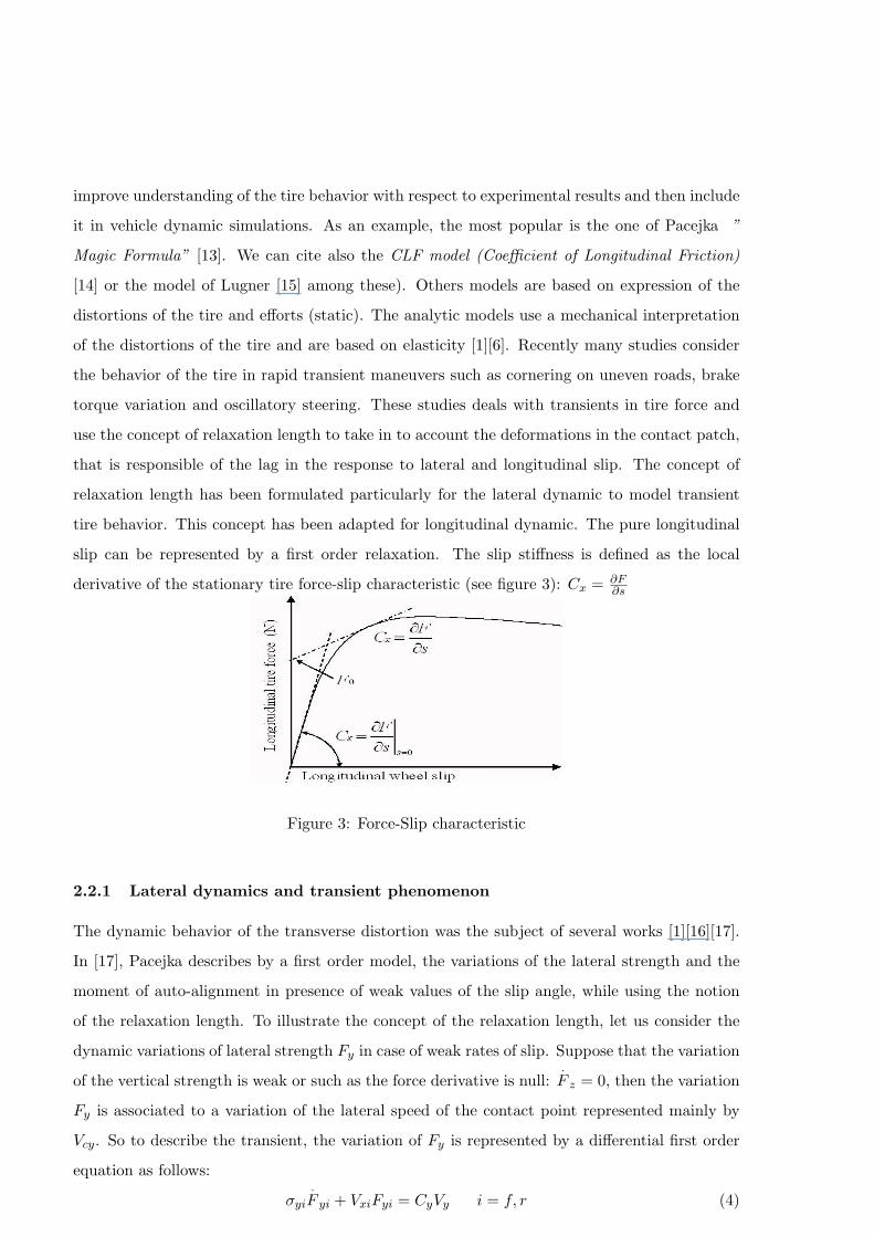
slip can be represented by a first order relaxation. The slip stiffness is defined as the local

derivative of the stationary tire force-slip characteristic (see figure 3): Cx = ∂F∂s

Figure 3: Force-Slip characteristic

2.2.1 Lateral dynamics and transient phenomenon

The dynamic behavior of the transverse distortion was the subject of several works [1][16][17].

In [17], Pacejka describes by a first order model, the variations of the lateral strength and the

moment of auto-alignment in presence of weak values of the slip angle, while using the notion

of the relaxation length. To illustrate the concept of the relaxation length, let us consider the

dynamic variations of lateral strength Fy in case of weak rates of slip. Suppose that the variation

of the vertical strength is weak or such as the force derivative is null:.F z = 0, then the variation

Fy is associated to a variation of the lateral speed of the contact point represented mainly by

Vcy. So to describe the transient, the variation of Fy is represented by a differential first order

equation as follows:

σyi

.F yi + VxiFyi = CyVy i = f, r (4)

4

where Cy is the rigidity of the lateral slip, and σy represents the relaxation length. This char-

acterizes the behavior around Fy = 0 at lateral force variation. We can extended the equation

to the case of large slips to get:

σyi

.F yi = −Vx(Fyi − Fyi0) + CyVy i = f, r (5)

The unknown nominal parameters Fyi0 are the intersection of the tangent line ∂Fyi

∂λyiand force

axis Fyi

2.2.2 Longitudinal dynamics and transient phenomenon

By analogy, the notion of relaxation length is used to describe the longitudinal dynamics. In

[3], the authors present the variations of the slip rate by a first order differential equation. The

longitudinal variation can be represented by the first order model:

σxi

.F xi = −Vx(Fxi − Fxi0) + Cx(Vx − riωi) i = f, r during the braking

σxi

.F xi = −riωi(Fxi − Fxi0) + Cx(Vx − riωi) i = f, r during the acceleration

2.2.3 Contact equations

Finally, the model can be represented, during acceleration phase, by:

.F xf = − Vx

σlfFxf +

Vx

σlfFxf0 +

Cx

σlfVx −

Cx

σlfrfωf

.F xr = − Vx

σlrFxr +

Vx

σlrFxr0 +

Cx

σlrVx −

Cx

σlrrrωr

.F yf =

Cy

σtfVy −

Vx

σtfFyf +

Vx

σtfFyfo (6)

.F yr =

Cy

σtrVy −

Vx

σtrFyr +

Vx

σtrFyro

2.2.4 VRIM

Let us define the following state variables. x1 = (x, y, ψ, αf , αr)T is the position vector and x2 =

(Vx, Vy,.ψ, ωf , ωr)T is the velocity vector. The force vector is noted x3 = (Fxf , Fxr, Fyf , Fyr)T .

The model can then be written in the state form as follows:.x1 = x2

.x2 = Ω(U)x3 +BU.x3 = Ψ(x2, x3)Θ

(7)

5

Where Ω(U) =

cos(δf )m

1m

− sin(δf )m 0

sin(δf )m 0 cos(δf )

m1m

lf sin(δf )Jz

0 lf cos(δf )Jz

−lrJz

−rf

Jf0 0 0

0 −rrJr

0 0

and B =

0 0 0

0 0 0

0 0 0

0 1/Jf 0

0 0 1/Jr

and U =

δf

Tf

Tr

The regression vector Ψ(X) is defined as follows, with A1 = Cxx21 − x21x31 − Cxrfx24 and

A2 = Cxx21 − x21x32 − Cxrrx25:

Ψ(X) =

A1 0 x21 0 0 0 0 0

0 A2 0 x21 0 0 0 0

0 0 0 0 Cyx22 − x33x21 0 x21 0

0 0 0 0 0 Cyx22 − x34x21 0 x21

In the model expression, we can introduce the parameters Θ = (θ1, θ2, θ3, θ4, θ5, θ6, θ7, θ8)T

as follows:

θ1 =1σlf

; θ2 =Fxf0

σlf; θ3 =

1σlr

; θ4 =Fxr0

σtr; θ5 =

1σlf

; θ6 =Fyf0

σtf; θ7 =

1σtr

; θ8 =Fyr0

σtr

3 Adaptive Estimation of Tire forces

3.1 Expression of the robust observer

The state vector is x = (x1, x2, x3) and the out put y = x2 (y ∈ R5) is the vector of measured

outputs of the system. To estimate both forces and velocities we propose the following observer

based on the sliding mode approach:[1][8].

x2 = Ω(U)x3 +BU +H2sign(x2 − x2).

x3 = Ψ(x2, x3)Θ +H3sign(x2 − x2)(8)

where xirepresent the observed state vectors, x2 = x2− x2, x3 = x3− x3 are the state estimation

errors. The observer gains Hi and the unknown parameter vector Θ will be defined thereafter.

The dynamics of the estimation errors can be written as:.

x2 = Ω(U)x3 −H2sign(x2).

x3 = Ψ(x2, x3)Θ−Ψ(x2, x3)Θ−H3sign(x2)(9)

In this observer we consider in fact only estimation of x2, x3 and the partial state x1 can be

obtained by integration of x2. The estimation error will be bounded, due to integration constant.

6

3.2 Convergence analysis

In order to study the observer stability, let us consider first the following Lyapunov function:

V2 =12xT

2 x2 (10)

The time derivative of V2 is given by.V 2 = xT

2

.

x2. According to equation (9), we can write:

.V 2 = xT

2 (Ω(U)x3 −H2sign(x2)) = xT2 Ω(U)x3 − xT

2H2sign(x2)

The involved forces are bounded, du to limitation of the system power. The a priori estimation

x3 is also bounded. Then we can consider that ‖x3‖ < µ; µ is a positive finite constant. By

chosing positvie matrix H2 (H2 > µΩ) we have.V 2 < 0, the surface x2 = 0 is then attractive,

leading x2 to converge towards x2 in a finite time t0 [7][8]. Moreover, in average we have.

x2 = 0

∀ t ≥ t0. Consequently we can deduce, that in average:

Ω(U)x3 −H2sign(x2) = 0 −→ x3 = Ω(U)+H2sign(x2) (11)

where Ω(U)+ is a pseudo inverse matix. Now, let us consider a second Lyapunov function:

V3 =12xT

3 x3 (12)

The time derivative is given by.V 3 = xT

3

.

x3 = xT3 (Ψ(x2, x3)Θ−Ψ(x2, x3)Θ−H3sign(x2))

from (9),.V 3 becomes:

.V 3 = (Ω(U)+H2sign(x2))T (Ψ(x2, x3)Θ−Ψ(x2, x3)Θ−H3sign(x2))

where∥∥∥(Ψ(x2, x3)Θ−Ψ(x2, x3)Θ

∥∥∥ < β

By considering the choice of gain H3 >> β we finally obtain:.V 3 < 0

So x3 goes to zero in finite time t1. Then,.

x3 −→ 0 therefore, Ψ(x2, x3)Θ − Ψ(x2, x3)Θ −

H3sign(x2) −→ 0

Owing to the fact that x2 = 0 and x3 = 0 ∀t > t1, we then have Ψ(x2, x3) = Ψ(x2, x3) and

then Ψ(x2, x3)(Θ− Θ) = H3sign(x2).

So we can conclude that the parameters can also by retrieved by construction

Θ = Θ + Ψ(x2, x3)−1H3signeq(x2)

4 Simulation results

In this section, we give some results in order to test and validate our approach an the proposed

observer. In simulation, the forces are generated by use of the Magic formula tire model.

The steering angle applied is shown in figure (4). The figure (5) and (6) show the convergence

of the estimated state vectors to their actual value in finite time. In figure (7) we show the

7

asymptotic convergence of the tire force to actual values. The performance of sliding mode

observer is satisfactory. The simulation results show that the adaptive observer is robust with

respect to parameters and model uncertainties and to the changes on the road conditions.

Figure 4: Steering Angle

Figure 5: Estimated and Measured States

Figure 6: Estimated and Measured States

8

Figure 7: Estimated and Measured Forces

5 Conclusion

In this paper, we have developed a new estimation method for vehicle dynamics based sliding

mode observer and an adequate simplified model. Simulation results are presented to illustrate

the ability of this approach to give estimation of both vehicle states and tire forces. The robust-

ness of the sliding mode observer versus uncertainties on the model parameters has also been

emphasized in simulation. This method will be applyed to an instrumented vehicle.

References

[1] H.B. Pacejka.: Simplified behaviour of steady state turning behaviour of motor vehilcles, part 2:

Stability of the steady state turn. Vehicle System Dynamics 2, 1973, pp. 173 - 183.

[2] Chia Shang Liu and Huei Peng. Road friction coefficient estimation for vehicle path prediction.

Vehicle System Dynamics, V 25 supl. 1996, pp413-425.

[3] C. L. Clover, and J. E. Bernard. Longitudinal Tire Dynamics. Vehicle System Dynamics, Vol. 29,

pp. 231-259, 1998.

[4] S. Drakunov, U. Ozguner, P. Dix and B. Ashrafi. ABS control using optimum search via sliding

modes. IEEE Trans. Control Systems Technology, V 3, pp 79-85, March 1995.

[5] J.Harned, L.Johnston, G.Scharpf. Measurement of Tire Brake Forces Characteristics as Related to

Wheel Slip (Antilock) Control System Design. SAE Transactions, Vol. 78, pp. 909-925, 1969.

[6] P. F. H. Dugoff and L. Segel. An analysis of tire traction properties and their influence on vehicle

dynamic performance. SAE Transaction, vol 3, pp. 1219-1243, 1970.

[7] L. Fridman and F. Castanos, ”Integral sliding mode control design via lyapunov methods for decen-

tralized control,” in Conference on Decision in Control 2004.b

9

[8] L. Fridman, ”Sliding mode control for systems with fast actuators: Singularly perturbed,” in Variable

Structure Systems: Toward the 21st century, X. Yu and J.-X. Xu, Eds. London, U.K.: Springer-

Verlag, 2002, vol. 274, Lecture Notes in Control and Information Science.

[9] Gentiane Venture. Identification des parametres dynamiques d’une voiture. These de Doctorat de

l’Ecole Polytechnique de l’Universite de Nantes, IRCCyN. Nantes novembre 2003.

[10] R. A. Ramirez Mendoza, Sur la Modelisation et la Commande des vehicules automobiles. Doctorat

de l’Institut National Polytechnique de Grenoble 1997.

[11] J. Ackermann ”Robust control prevents car skidding. IEEE Control systems magazine, vol. 17, n3,

pp. 23-31, june 1997. gn. SAE Trans. V78, pp909-925, 1969.

[12] H.Lee and M.Tomizuka. Adaptative vehicle traction force control for intelligent vehicle highway

systems (IVHSs) IEEE Trans. on Industrial Electronics, V 50 N 1 February 2003

[13] H.B.Pacejka, I.Besseling. Magic Formula Tyre Model with Transient Properties. 2nd Int Col on Tyre

Models for Vehicle Dynamic Analysis, Berlin 1997. Swets and Zeitlinger

[14] G. Beurier, Y. Delanne. Transposition de performances longitudinales de pneumatique - methode

de recherche statistique de relations entre les parametres de modeles en vue de l’identification de

ces parametres. CIFA2000.

[15] M. Gipser, R. Hofer, P. Lugner. Dynamical tyre forces response to road unevennesses. Vehicle System

Dynamics Supplement 27 (1997) pp 94-108

[16] H.B. Pacejka.: Simplified behaviour of steady state turning behaviour of motor vehilcles, part 1:

Handling diagrams and simple systems. Vehicle System Dynamics 2, 1973, pp. 162 - 172.

[17] Pacejka, H.B., Besseling, I.: Magic Formula Tyre Model with Transient Properties. 2nd International

Tyre Colloquium on Tyre Models for Vehicle Dynamic Analysis, Berlin, Germany (1997). Swets and

Zeitlinger.

10