Valdez-Mondragón, A. & O. F. Francke. 2015. Phylogeny of the spider genus Ixchela Huber, 2000...

Phylogeny of the spider genus Ixchela Huber, 2000(Araneae: Pholcidae) based on morphological andmolecular evidence (CO1 and 16S), with a hypothesizeddiversification in the Pleistocene

ALEJANDRO VALDEZ-MONDRAGÓN1,2* and OSCAR F. FRANCKE1

1Colección Nacional de Arácnidos (CNAN), Instituto de Biología, Universidad Nacional Autónoma deMéxico (UNAM), Apartado Postal 70-153, C. P. 04510, Ciudad Universitaria, Coyoacán, DF, MexicoCity, Mexico2Alexander Koenig Research Museum of Zoology, Adenauerallee 160, 53113 Bonn, Germany

Received 17 July 2014; revised 8 February 2015; accepted for publication 10 February 2015

The genus Ixchela Huber is composed of 20 species distributed from north-eastern Mexico to Central America,including the five new species described here from Mexico: Ixchela azteca sp. nov., Ixchela jalisco sp. nov.,Ixchela mendozai sp. nov., Ixchela purepecha sp. nov. and Ixchela tlayuda sp. nov. We test the monophylyand investigate the phylogenetic relationships among species of the genus Ixchela using morphological and mo-lecular data. Parsimony (PA) analysis of 24 taxa and 40 morphological characters with equal and implied weightssupported the monophyly of Ixchela with eight morphological synapomorphies. The PA analyses with equal andimplied weights, and separate Bayesian inference (BI) analyses for the CO1 gene (506 characters), concatenatedgene fragments CO1 + 16S (885 characters), morphology + CO1 (546 characters) and the combined evidence dataset (morphology + CO1 + 16S) (925 characters) support the monophyly of Ixchela. Our preferred topology showstwo large clades; clade 1 has a natural distribution in the Mesoamerican biotic component, whereas clade 2 pre-dominates in the Mexican Montane biotic component. The genus Ixchela diverged in the late Miocene, and thedivergence between the internal clades in the genus occurred in the late Pliocene; by contrast, most of the spe-ciation events seem to have occurred mainly during the Pleistocene, where climatic changes brought on by re-peated glaciations played an important role in the diversification of the genus.

© 2015 The Linnean Society of London, Zoological Journal of the Linnean Society, 2015doi: 10.1111/zoj.12265

ADDITONAL KEYWORDS: Bayesian inference – historical biogeography – molecular clocks – morphology– parsimony – phylogeny – taxonomy.

INTRODUCTION

The spider family Pholcidae C. L. Koch, 1850 con-sists of five subfamilies: Ninetinae Simon, 1890;Arteminae Simon, 1893; Modisiminae Simon, 1893;Smeringopinae Simon, 1893; and Pholcinae C. L. Koch,1850 (Huber, 2011a). The subfamily Modisiminae cur-rently includes 412 species grouped in 33 genera, someof which are speciose (e.g. Anopsicus Chamberlin &

Ivie, 1938; Psilochorus Simon, 1893; Modisimus Simon,1893, Mesabolivar González-Sponga, 1998); and manyundescribed species are known (Huber, 2011a). Al-though some clades have been identified within thesubfamily, the phylogenetic relationships withinModisiminae are not yet completely resolved. Thereare some clades within Modisiminae that are morpho-logically supported (Huber, 1998b, 2011a). Although pre-vious molecular data do not support the monophylyof the subfamily (Huber & Astrin, 2009), recent studiesusing seven genes support the monophyly ofModisiminae with some changes in the internal*Corresponding author. E-mail: [email protected]

Zoological Journal of the Linnean Society, 2015. With 15 figures

© 2015 The Linnean Society of London, Zoological Journal of the Linnean Society, 2015 1

mailto:[email protected]

phylogenetic relationships (Dimitrov, Astrin & Huber,2012).

Dimitrov et al. (2012) found that based on molecu-lar dating, the subfamily Modisiminae, which in-cludes the genus Ixchela, diverged approximately140 Mya, and that some lineages are present in bothNorth and South America. Raising of the Panamaisthmus around 3.5 Mya (Coates et al., 1992) appearsto have allowed the geographical expansion of pholcidsfrom North America into South America and vice versa(e.g. Metagonia (Pholcinae) and Psilochorus(Modisiminae)). However, recent studies using sevengenes found that Psilochorus is not monophyletic(Dimitrov et al., 2012), and consisted of two differentlineages, one North American (including the Carib-bean Islands) and another South American. This sup-ports the idea that the composition of pholcids fromNorth America and South America is completely dif-ferent, and that there has not been a geographical ex-pansion from North America to South America in thisgroup or vice versa.

The spider genus Ixchela Huber, 2000 was origi-nally composed of only five species (Pickard-Cambridge,1898, 1902; Gertsch, 1971) until Valdez-Mondragón(2013) described nine new species from Mexico and onefrom Honduras, raising the known diversity to 15 de-scribed species. The genus Ixchela has a natural dis-tribution in temperate climate zones, in pine, oak orpine–oak forest at moderately high altitudes (1000–2950 m). The natural distribution pattern of Ixchelarenders it an excellent model to explore the patternsof speciation and diversification found in temperatemontane forests in Mexico, which have been hypo-thetically triggered by the climatic oscillations asso-ciated with the Pleistocene glaciations (Zarza, Reynoso& Emerson, 2008; Rícan et al., 2013; Pedraza-Lara et al.,2015). This work represents the first attempt to explainthe pattern of speciation and diversification in tem-perate forest spiders in Mexico.

The monophyly of Ixchela has not previously beentested. Originally, when this genus was proposed it wassupported by only one character, the distinctiveprolateroventral apophysis on the palp bulb of the male(Huber, 1998a, 2000; Valdez-Mondragón, 2013). In ad-dition, the phylogenetic relationships between Ixchelaand other genera of the subfamily Modisiminae arenot clear. Huber (2000), however, mentioned that al-though Ixchela resembles Aymaria Huber, 2000 in overallshape, it is only superficial similarity and notsynapomorphies that link the two genera, or that linkIxchela with any other sister genus within Modisiminae(Huber, 2011a). Recently, an updated phylogenetic analy-sis of the whole family, including Ixchela for the firsttime, found that the genus was closely related toPsilochorus from North America, supporting the hy-pothesis that the North American and South Ameri-

can species of Psilochorus do not belong in a monophyleticclade (Dimitrov et al., 2012, in prep.).

Here, we present the first phylogenetic analysis ofthe genus Ixchela Huber, 2000, testing its monophylywith different sets of data, using morphology and frag-ments of two mitochondrial genes (CO1 and 16S). Wegenerated nucleotide sequences from those twomitochondrial genes, which were selected because theirsubstitution rates allow the establishment of relation-ships at the species level, as shown by previousphylogenetic analyses in spiders and other arthropodgroups, including Pholcidae (e.g. Hebert et al., 2003a;Hebert, Ratnasingham & deWaard, 2003b; Arnedo et al.,2004; Bruvo-Madaric et al., 2005; Astrin et al., 2006;Álvarez-Padilla et al., 2009; Hendrixson et al., 2013).In addition, this study presents a phylogenetic hy-pothesis with an estimation of lineage divergence timesfor Ixchela and their 95% highest posterior density in-terval (HPD) using molecular evidence, based on arelaxed molecular clock. We also discuss the diver-gence time within the context of historical biogeo-graphical and geological complexity of Mexico, mainlyin temperate climate zones. Finally, we describe fivenew species as a result of the taxonomic revision ofthe genus Ixchela (Valdez-Mondragón, 2013), and presentnew morphological and biogeographical data for thegenus.

MATERIAL AND METHODSBIOLOGICAL MATERIAL

We examined specimens deposited in the followingmuseums and institutions: Colección Nacional deArácnidos, Instituto de Biología, Universidad NacionalAutónoma de México, Mexico City (CNAN); UniversidadMichoacana de San Nicolás de Hidalgo, Michoacán,Mexico (UMSNH); American Museum of NaturalHistory, New York, USA (AMNH); Texas MemorialMuseum, University of Texas, Austin, Texas, USA (TMM-UT); Instituto Nacional de Biodiversidad, Santo Domingode Heredia, Costa Rica (INBio). The specimens wereexamined with a Nikon SMZ645 stereoscopic micro-scope. All measurements are in millimetres (mm).Female epigyna and male palps were dissected inethanol (80%) and cleared in potassium hydroxide (KOH,10%) for 5 min. Photographs were taken with a NikonCoolpix S10 VR camera with a Martin Microscopeadapter. Morphological structures were suspended in96% gel alcohol to facilitate positioning and coveredwith a thin layer of liquid ethanol (80%) to minimizediffraction during photography. For the photomicro-graphs, the morphological structures were dissectedand cleaned with an ultrasonic cleaner at 20–40 kHz;subsequently they were critical-point dried, andexamined at low vacuum in a Hitachi S-2460N

2 A. VALDEZ-MONDRAGÓN AND O. F. FRANCKE

© 2015 The Linnean Society of London, Zoological Journal of the Linnean Society, 2015

scanning electron microscope. All scale measure-ments on photomicrographs are in micrometres (μm).The maps were prepared with ArcView GIS version3.2 (Applegate, 1999). The photographs and maps wereedited using Adobe Photoshop Version 7.0. Abbrevia-tions: ALE, anterior lateral eyes; AME, anterior medianeyes; FAC, frontal apophysis of chelicerae; MSE, medianseptum of epigynum; PAB, prolateroventral apophysisof bulb; PLE, posterior lateral eyes; PME, posteriormedian eyes; PP, pore plates; SAC, sclerotized apophysisof chelicerae; VAE, ventral apophysis of epigynum; VAF,ventrodistal apophysis of femur; VPP, ventrobasal pro-tuberance of procursus.

TAXON SAMPLING

The cladistic analyses presented here are based on 32taxa. The species used in the molecular analyses arelisted in Table 1. The in-group includes 20 species ofIxchela [15 species described or redescribed byValdez-Mondragón, (2013) and five new species de-scribed herein]. Outgroups for the morphological analy-sis include Physocyclus dugesi Simon, 1893; Prisculabinghamae (Chamberlin, 1916); ‘Coryssocnemis’ ivieGertsch, 1971; and Aymaria conica (Banks, 1902) (Ap-pendix 2). Outgroups for molecular analyses includeP. dugesi; Carapoia paraguaensis González-Sponga, 1998;Mesabolivar luteus (Keyserling, 1891); P. binghamae;

Table 1. Specimens sequenced for each species, DNA voucher numbers, localities, and GenBank accession numbers

SpeciesDNA voucherCNAN* Locality

GenBank accession number

CO1 16S

Ixchela abernathyi (Gertsch) Ara0238 MEXICO: San Luis Potosí KF150114 KF178420Ixchela franckei Valdez-Mondragón Ara0164 MEXICO: Guerrero KF150084 KF178390Ixchela furcula (F. O. Pickard-Cambridge) Ara0316 GUATEMALA: Sacatepequez KF150127 KF178433Ixchela grix Valdez-Mondragón Ara0235 MEXICO: Oaxaca KF150111 KF178417Ixchela huasteca Valdez-Mondragón Ara0194 MEXICO: Querétaro KF150101 KF178407Ixchela huberi Valdez-Mondragón Ara0190 MEXICO: Oaxaca KF150098 KF178404Ixchela juarezi Valdez-Mondragón Ara0218 MEXICO: Oaxaca KF150108 KF178414Ixchela mixe Valdez-Mondragón Ara0173 MEXICO: Oaxaca KF150090 KF178396Ixchela pecki (Gertsch) Ara0308 MEXICO: Chiapas KF150125 KF178431Ixchela placida (Gertsch) Ara0201 MEXICO: Veracruz KF150105 KF178411Ixchela santibanezi Valdez-Mondragón Ara0309 MEXICO: Chiapas KF150126 KF178432Ixchela simoni (O. Pickard-Cambridge) Ara0320 MEXICO: Guerrero KF150129 KF178435Ixchela taxco Valdez-Mondragón Ara0273 MEXICO: Guerrero KF150089 KF178395Ixchela tzotzil Valdez-Mondragón Ara0303 MEXICO: Chiapas KF150123 KF178429Ixchela viquezi Valdez-Mondragón Ara0319 HONDURAS: Fco. Morazán KF150128 KF178434Ixchela azteca sp. nov. Ara0158 MEXICO: Distrito Federal KF150079 KF178385Ixchela jalisco sp. nov. Ara0328 MEXICO: Jalisco KF150131 KF178437Ixchela mendozai sp. nov. Ara0326 MEXICO: Puebla KF150130 KF178436Ixchela purepecha sp. nov. Ara0253 MEXICO: Michoacán KF150119 KF178425Ixchela tlayuda sp. nov. Ara0225 MEXICO: Oaxaca KF150097 KF178403Outgroups

Coryssocnemis simla Huber GenBank VENEZUELA: Sucre AY560773 DQ667753Carapoia paraguaensis González-Sponga GenBank VENEZUELA: El Dorado DQ667855 DQ667749Mesabolivar luteus Huber GenBank BRAZIL: Minas Gerais DQ667873 DQ667766Modisimus macaya Huber & Fischer GenBank HAITI: Macaya B. R. FJ228029 FJ227994Modisimus seguin Huber & Fischer GenBank HAITI: nr Seguin FJ228026 FJ227992Physocyclus dugesi Simon GenBank COSTA RICA: San Pedro de

Montes de OcaAY560787 –

Physocyclus globosus (Taczanowski) GenBank GUATEMALA: Lívingston – DQ667821Priscula binghamae (Chamberlin) GenBank BOLIVIA: La Paz DQ667932 DQ667826Psilochorus simoni (Berland) GenBank GERMANY: Bonn AY560789 –Tainonia serripes (Simon) GenBank DOMINICAN REPUBLIC:

NE ParaisoFJ799790 FJ799777

*Vouchers of all species of the in-group are deposited in Colección Nacional de Arácnidos (CNAN), Institute of Biology,UNAM, Mexico.

PHYLOGENY OF IXCHELA 3


Coryssocnemis simla Huber, 2000; Modisimus macayaHuber & Fischer, 2010; and Modisimus seguin Huber& Fischer, 2010. The outgroup taxa were selected basedon previous analyses of phylogenetic relationships ofthe family Pholcidae (Huber, 2000, 2011a; Dimitrov et al.,2012). Outgroup sequences were retrieved fromGenBank.

MORPHOLOGICAL DATA

The morphological matrix comprises 40 characters, 34binary and six multistate (Appendix 1). Thirty-two char-acters were potentially informative and eight were un-informative. In the analyses with equal and impliedweighting, uninformative characters were deactivat-ed to avoid inflating the tree length (L) and consist-ency index (CI) (Goloboff, 1993, 1995). The matrix wascreated in WinClada–Asado, version 1.7 (Nixon, 2004).Multistate characters were considered non-additive(Fitch, 1971).

DNA EXTRACTION, AMPLIFICATION AND SEQUENCING

DNA extractions varied depending on the available ma-terial and on the specimens’ body size. DNA was iso-lated from the prosoma (juv.), opisthosoma (juv.) or halfopisthosoma (adults), complete legs (juv.), leg femuror half leg femur (adults), femur + patella + tibia (juv.),or in some cases from the whole individual spider (smalljuv.). DNA extractions were done using a Qiagen DNeasyTissue Kit. Extractions were verified by electrophore-sis in 1% agarose gel (100 mL TBE + 1 g agarose; Sigma-Aldrich), using a ladder marker of 100 bp. DNAfragments corresponding to approximately 600 bp ofthe cytochrome c oxidase subunit 1 (CO1) gene andapproximately 440 bp of the 16S ribosomal RNA genewere obtained. The fragments were amplified using theprimers shown in Table 2.

Amplifications were carried out in an AppliedBiosystems Thermal Cycler model 2720, in a totalvolume of 25 μL containing 2.5 μL DNA, 2.5 PCR 10×buffer, 1.5 μL MgCl2, 1.0 μL dNTPs, 0.5 μL of molecu-lar marker for CO1 and 1 μL for 16S, 16 μL H2O forCO1 and 15 μL for 16S, and 0.5 μL Taq PCR Core poly-merase (Qiagen). The PCR programme for CO1 wasas follows: amplification of COI consisted of 30 cyclesof 20 s at 94 °C, 20 s at 48 °C and 40 s at 72 °C (Huber,

Fischer & Astrin, 2010). Amplification of 16S consist-ed of two cycles: the first cycle of 7–9 repeats of 30 sat 94 °C, 30 s at 55 °C (−1 °C per cycle) and 50 s at72 °C; the second cycle of 23 repeats of 30 s at 94 °C,30 s at 50 °C and 50 s at 72 °C (Astrin et al., 2006).PCR products were checked to analyse length and purityon 1% agarose gels and purified directly from the PCRmixture using a Millipore Amicon-Ultra 0.5-μL Cen-trifugal Filters Kit; purifications were checked onagarose gels with a marker of 100 bp. DNA extrac-tion, amplification and sequencing were performed atthe Molecular Laboratory at the Instituto de Biología,Universidad Nacional Autónoma de México (UNAM),Mexico City. Sequencing of both strands (5′–3′ and 3′–5′) of PCR products were done in a Genetic AnalyzerRUO Applied Biosystems Hitachi model 3500xL. Se-quence data are deposited in GenBank (http://www.ncbi.nlm.nih.gov/genbank/) with accession numbers:KF150079–KF150131 for CO1, and KF178385–KF178437 for 16S (Table 1).

DNA SEQUENCE ALIGNMENT AND EDITION

Sequences were aligned using the default Gap openingpenalty of 1.53 in MAFFT (Multiple sequences Align-ment based on Fast Fourier Transform), version 6(Katoh & Toh, 2008), available online, using the fol-lowing alignment strategy: Auto (FFT-NS-2, FFT-NS-i or L-INS-i; depending on data size). The gaps weretreated as missing data. Inspection and editing of se-quences and alignments were done using BioEdit version7.0.5.3 (Hall, 1999). The BioEdit matrices were ex-ported to WinClada–Asado, version 1.7 (Nixon, 2004).The matrices obtained from the multiple sequence align-ments were then used in both parsimony (PA) andBayesian inference (BI) analyses.

PHYLOGENETIC ANALYSES

Phylogenetic analyses were performed using PA withNONA version 1.7 (Nixon, 2004), and BI was per-formed using MrBayes version 3.1 (Huelsenbeck &Ronquist, 2001). PA and BI were conducted using theWinClada–Asado interface. The BI consensus tree wasselected using default settings. Partition-homogeneitytests (incongruence length difference test) were doneto analyse congruence between partitions (CO1, 16S

Table 2. Primers used for PCR

Gene Primer name Primer sequence (5′–3′) Reference

CO1 LCO1490 GGTCAACAAATCATAAAGATATTGG Folmer et al. (1994)HC02198 TAAACTTCAGGGTGACCAAAAAATCA

16S rRNA 16sar-5′ CGCCTGTTTATCAAAAACAT Hillis, Moritz & Mable (1996)1 6sbr-3′ CCGGTCTGAACTCAGATCACGT



http://www.ncbi.nlm.nih.gov/genbank/

http://www.ncbi.nlm.nih.gov/genbank/

and morphology). PA and BI analyses were applied foreach separate matrix as well as for the combined evi-dence. Ambiguous optimizations were resolved usingaccelerated transformation (ACCTRAN) to explainhomoplasy on the topologies (Farris, 1970; Swofford& Maddison, 1987; Agnarsson & Miller, 2008). We se-lected ACCTRAN because some clades were morestrongly supported with additional synapomorphies. Thetrees were edited with WinClada–Asado and AdobePhotoshop 7.0. In NONA, the analyses with equalweighting were conducted using the following com-mands: Maximum trees to keep (hold) = 10 000; No.of replications (mult*N) = 1000; Starting trees per rep(hold/) = 50; using Multiple TBR + TBR (mult*max*).

The implied character weighting used on the mor-phological and molecular analyses was conducted toanalyse the effects of homoplasy on tree topologies. PAanalyses with implied weighting were done using tra-ditional searches with TNT (Goloboff, Farris & Nixon,2008) with the following commands: Starting trees usingWagner trees: Random seed = 1000; Replications (Numberof add. seqs.) = 1000; Swapping algorithm (TBR): treesto save per replication = 100. Seven arbitrary concav-ity values were used: K = 1, 2, 3, 4, 5, 9 and 10.

Symmetric resampling (SR) (Goloboff et al., 2003)support values were used under implied weightings toavoid the under- or overestimations usually generat-ed with Jackknife values when the characters have dif-ferent weights or some state transformation costs aredifferent, as proposed by Goloboff et al. (2003). For equalweighting analyses, Jackknife and Bremer supportvalues (Bremer, 1988) were applied. The Jackknifevalues were calculated with the following commands:Number of replicates = 1000; Search trees with tradi-tional search; only the statistically significant values≥ 64% are shown on the trees. The Bremer values werecalculated with the following commands: Retains treessuboptimal: 20 steps (morphological data), 40 steps (mo-lecular data); Nodes were collapsed when support wasless than 1; Type of support: absolute support; Cal-culate supports with existing suboptimal trees. The SRvalues were calculated with the following commands:Number of replicates = 1000; Search trees with tradi-tional search; only the statistically significant values≥ 67% were considered.

The models of sequence evolution were selected usingthe best-fit partitioning scheme with PartitionFinderversion 1.1.1 (Lanfear et al., 2012, 2014), using theAkaike information criterion (AIC) (Posada & Buckley,2004). Under PartitionFinder, CO1 alignment wasdefined as three data blocks, corresponding to each codonposition; and 16S was defined in a single data block.The models selected for CO1 for each partition blockwere: GTR + I + G (1st and 2nd codon positions) andGTR + G (3rd position). For 16S the model selected wasGTR + G. BI analyses with four parallel Markov chains

were run with the following commands: MCMC gen-erations = 10 000 000; sampling frequency = 200; printfrequency = 200; number of runs = 2; number ofchains = 4; MCMC burnin = 2500; sumt burnin = 2500;sump burnin = 2500. TRACER version 1.5 (Rambaut& Drummond, 2003–2009) was used to analyse the pa-rameters and the effective sample size (ESS) of theMarkov Chain Monte Carlo (MCMC) method.

MOLECULAR DATING

We used jModelTest (Posada, 2008) to test the use ofa strict molecular clock to date divergence times withinIxchela; however, this model was statistically reject-ed by the likelihood ratio test (LRT) (Huelsenbeck &Crandall, 1997). Therefore, we used the relaxeduncorrelated lognormal clock model implemented usingthe programs BEAUti (Bayesian Evolutionary Analy-sis Utility) version 1.7.5 (Drummond, Xie & Heled, 2012)and BEAST (Bayesian Evolutionary Analysis Sam-pling Trees) version 1.7.5 (Drummond et al., 2012). Theinterval of the lineage divergence times for the genusIxchela and their internal relationships were estab-lished calculating their 95% HPD to each tmrca (timeof the most recent common ancestor) in each node. Al-though there are no fossils of Ixchela to calibrate themolecular clock, our calibration was based on the fossilrecord of the subfamily Modisiminae described byWunderlich (1988) from Dominican amber (where sixfossil species of the genus Modisimus were described);thus, our calibration point is based on the dating ofthe Dominican amber (15 Mya) (Neogene) (Poinar, 1992;Iturralde-Vinent, 2005). The value of 15 Mya was usedto calibrate as mean in prior section of BEAUTi, usinga normal distribution with a standard deviation of 1.We used the CO1 + 16S matrix to calculate the diver-gence times to calibrate the relaxed clock and esti-mate lineage divergence times and their 95% HPD. Forthe molecular dating, we selected two extant speciesof Modisimus from Hispaniola, namely M. macaya andM. seguin, both from Haiti, selected because they aredistributed on the same island where the Dominicanamber with the fossil species of Modisimus were found.Although this fossil record is young, we used it becauseof the scarcity of fossil material for the family, andbecause Modisimus is the only genus in the subfam-ily Modisiminae with a fossil record. The results underthe molecular clock with lognormal relaxed clock modelfor the tmrca were analysed posteriorly using TRACERto evaluate the parameters and the ESS of the MCMC.TRACER and TreeAnnotator version 1.7.5. (Rambaut& Drummond, 2002–2013) were further used to selectthe number of generations with low posterior prob-abilities discarded as burn-in (25%). The parametersused in BEAUti for the analysis with BEAST were asfollows: Model = Lognormal relaxed clock (Uncorrelated),



estimate; Tree Prior = Speciation: Yule Process, witha random starting tree; Substitution and Site Hetero-geneity model = GTR + I + G; Base frequencies = Em-pirical; Number of Gamma Categories = 4; MCMC lengthof chain = 20 000 000.

RESULTSTAXONOMY

Pholcidae C. L. KOCH, 1850

Ixchela HUBER, 2000

Type species: Ixchela furcula (F. O. Pickard-Cambridge,1902) by original designation (Huber, 2000). Type lo-cality: 1 female holotype from Tecpam in the Regiónde Los Altos (Tecpam, Departamento Chimaltenango),Guatemala, around 2300 m, Godman & Salvin Cols.,in BMNH (F. O. Pickard-Cambridge, 1902; Huber,1998a) (not examined).

Diagnosis: Species of this genus can be distinguishedfrom members of other pholcid genera by the frontalapophysis on chelicerae on males (FAC) (Figs 26, 40,51); the prolateroventral apophysis of the palp bulbof the male (PAB) (Figs 1, 39, 50); the apical–dorsalspine-shaped projection on the embolus (Figs 2, 38, 49);the apical–ventral projection on the embolus (Figs 2,38, 49); the curved spine distally on procursus (Figs 38,49, 60); the ventral protuberance with long setae onthe procursus (VPP) (Figs 15, 38, 49); the procursusconical, straight and long, wide basally (Figs 60, 72);and the small, sub-distal, sclerotized spine on theembolus (Figs 9, 39, 50).

Description: The description made by Valdez-Mondragón(2013) is currently still valid, although new morpho-logical information has been found using scanning elec-tron microscopy (SEM). Embolus conical (Fig. 1), withelongate, sigmoid apical ventral projection (Figs 2, 4,6), and apical dorsal projection spine-shaped (Fig. 2).Sperm operculum with a small spine (arrow, Fig. 3).Embolus with small, spine-shaped projectionsprolaterally (e.g. I. azteca, arrow Figs 4, 5; andI. mendozai, arrow Figs 7–9). Embolus with sub-distal, sclerotized spine (arrow, Fig. 9). Female palpwith long and wide seta next to the tarsal organ (arrow,Fig. 13). Bulb rounded and wide (Fig. 1). Tarsal organsexposed on palps (arrows, Figs 16, 17) and legs (arrow,Figs 24, 25). Trichobothria present on palp tibia of malesand females (Figs 10–12). Lyriform organs present onleg patellae (arrow, Figs 18, 19). Legs with 6–9 lon-gitudinal rows of erect setae, spread around circum-ference of segments (Figs 20, 21), without spines orcurved setae. Tarsus IV with comb-setae (Figs 22, 23).Male chelicerae with SAC well developed in some species(e.g. I. azteca, I. mendozai) (Figs 26, 27), vestigial in

others (e.g. I. simoni, I. tzotzil) (Valdez-Mondragón, 2013;figs 74, 162); or absent (e.g. I. furcula, I. huberi)(Valdez-Mondragón, 2013; figs 34, 100). Endites withserrated margin (arrow, Figs 29, 30). Anterior lateralspinnerets with one small spigot and one wide spigot(arrows, Fig. 32). Posterior median spinnerets with twoacciniform gland spigots (arrows, Fig. 33).

Distribution and natural history: New data on the naturalhistory were obtained and are explained, although thegeneral distribution and natural history of the genusgiven by Valdez-Mondragón (2013) is still the same.The genus Ixchela Huber, 2000 is widely distributedfrom north-eastern Mexico to Nicaragua [specimens notexamined, but Huber (2000) examined one male of anundescribed species from Nicaragua, Matagalpa, FuentePura, deposited in Museo Entomológico Nicaraguense](Valdez-Mondragón, 2013). The genus has a naturaldistribution in temperate climate zones, particularlypine, oak or mixed pine–oak forest (1000–2950 m el-evation) (Valdez-Mondragón, 2013; figs 13–15, 17, 18);however, some species were collected in tropical rainforest, such as Ixchela santibanezi Valdez-Mondragón,2013 at 1190 m (Valdez-Mondragón, 2013; fig. 16), orin a thorny scrub forest at 1900–2180 m, such as Ixchelajuarezi Valdez-Mondragón, 2013. Most species have beencollected among fallen logs, boulders on the ground,under dried leaves of agave plants and frequently onwalls along road-cuts, specifically in dark, moist areascovered with roots and leaf-litter (Valdez-Mondragón,2013; figs 15, 17, 18), or inside caves (Valdez-Mondragón,2013; figs 1–3, 5, 9). However, here three synanthropicrecords for the genus are reported for the first time:two records of Ixchela azteca and one record of Ixchelamendozai found inside buildings.

Composition: The genus Ixchela is composed of 20species: Ixchela simoni (O. Pickard-Cambridge, 1898),Ixchela furcula (F. O. Pickard-Cambridge, 1902), Ixchelaabernathyi (Gertsch, 1971), Ixchela pecki (Gertsch, 1971),Ixchela placida (Gertsch, 1971), Ixchela franckeiValdez-Mondragón, 2013, Ixchela grix Valdez-Mondragón,2013, Ixchela huasteca Valdez-Mondragón, 2013,Ixchela huberi Valdez-Mondragón, 2013, Ixchelajuarezi Valdez-Mondragón, 2013, Ixchelamixe Valdez-Mondragón, 2013, Ixchela santibaneziValdez-Mondragón, 2013, Ixchela taxco Valdez-Mondragón, 2013, Ixchela tzotzil Valdez-Mondragón,2013, Ixchela viquezi Valdez-Mondragón, 2013, Ixchelaazteca sp. nov., Ixchela jalisco sp. nov., Ixchela mendozaisp. nov., Ixchela purepecha sp. nov. and Ixchela tlayudasp. nov.

The identification key of species of Ixchela Huber,2000 is updated from Valdez-Mondragón (2013 – here-after VM, 2013), using the same abbreviations.



Figures 1–9. Ixchela azteca sp. nov. (1–6) and Ixchela mendozai sp. nov. (7–9). 1, Left palp showing bulb, PABand embolus, prolateral view. 2, 3, Embolus, prolateral–dorsal view (arrow indicates the spine on sperm duct). 4, 6, Embolus,prolateral and retrolateral views, respectively (arrow indicates the spine-shaped projections). 5, 7, Details of the spine-shaped projections on embolus. 8, Embolus, distal view (arrow indicates the spine-shaped projections). 9, Embolus, retrolateralview (arrow indicates the sub-distal, sclerotized spine). Scale bars: 30 μm (Fig. 7), 50 μm (Fig. 5), 100 μm (Figs 3, 8, 9),200 μm (Figs 2, 4, 6), 500 μm (Fig. 1).



IDENTIFICATION KEY

Males1. Chelicerae with well-developed SAC (Figs 37, 48, 59).......................................................................2• Chelicerae without or with inconspicuous SAC (VM, 2013; figs 34, 74, 100)........................................112 (1). Chelicerae with FAC long (Figs 40, 51, 74).....................................................................................4• Chelicerae with FAC small (VM, 2013; figs 150, 205) .......................................................................33 (2). Chelicerae with FAC wide basally with tip slightly curved (VM, 2013; figs 149, 150); embolus with basal pro-

tuberance conical, ending in round tip near PAB (VM, 2013; figs 153, 154); palp with small PAB (VM, 2013;figs 153, 154); palp femur wide and short, 2× longer than wide (VM, 2013; figs 152, 153); procursus withlong distal spine, curved basally and straight distally (VM, 2013; figs 152, 153)................................................................................................................................Ixchela franckei Valdez-Mondragón

• Chelicerae with FAC small and with tip not curved (VM, 2013; figs 204, 205); embolus without basal protu-berance (VM, 2013; fig. 208); palp with large PAB (VM, 2013; figs 207, 208); palp femur thin and long, almost3× longer than wide (VM, 2013; figs 207, 208); procursus with long distal spine, straight basally and curveddistally, J-shaped (VM, 2013; figs 207–209) ...................................Ixchela viquezi Valdez-Mondragón

4 (2). Palp femur without ventral protuberances (Fig. 38, 49), chelicerae with FAC straight, located on basal third(Figs 40, 51)..............................................................................................................................5

• Palp femur with a ventral conical protuberance (VM, 2013; arrow fig. 140); chelicerae with FAC curved, locatedbasally (VM, 2013; figs 136, 137) ................................................... Ixchela taxco Valdez-Mondragón

5 (4). FAC pointed apically (VM, 2013; figs 22, 63)...................................................................................6• FAC rounded apically (Figs 62, 85) ............................................................................................... 96 (5). Palp femur convex ventrally (Figs 38, 49) ...................................................................................... 7• Palp femur concave ventrally (VM, 2013; figs 25, 65) .......................................................................87 (6). FAC wide and conical, directed toward front (Figs 37, 40); VAF small (Figs 38, 39); colour pattern around

the fovea very marked, width even throughout (Fig. 35) ...................................Ixchela azteca sp. nov.• FAC very long, directed upward and slightly curved apically (Figs 48, 51); VAF long and curved (Figs 49,

50); colour pattern around the fovea diffuse, wider anteriorly (Fig. 46)................Ixchela jalisco sp. nov.8 (7). Retrolateral face of palp femur with several setae medially (VM, 2013; fig. 25); PAB straight and wide, without

a distinct notch between PAB and embolus (VM, 2013; fig. 26).................Ixchela abernathyi (Gertsch)• Retrolateral face of palp femur without setae medially (VM, 2013; fig. 65); PAB narrow and curved, with a

distinct notch between PAB and embolus (VM, 2013; fig. 66).........................Ixchela placida (Gertsch)9 (6). FAC forming an angle of > 90° with the chelicerae in lateral view....................................................10• FAC forming an angle of 90° with the chelicerae in lateral view, (Fig. 62).......Ixchela mendozai sp. nov.10 (9). FAC distally ending in a small tip (Fig. 85)..................................................Ixchela tlayuda sp. nov.• FAC distally rounded (Fig. 74) ............................................................... Ixchela purepecha sp. nov.11 (1). FAC with frontal and curved sclerotized apophyses (VM, 2013; figs 50, 89, 176)..................................12• FAC without frontal and curved sclerotized apophyses....................................................................1412 (11). PAB small and non-protruding (VM, 2013; figs 54, 181); curved sclerotized apophyses on FAC long, claw-

shaped, pointing forward (VM, 2013; figs 49, 175)..........................................................................13• PAB strongly developed, distinctly protruding (VM, 2013; fig. 92); curved sclerotized apophyses on FAC short,

hook-shaped, pointing towards each other (VM, 2013; figs 88–90).........Ixchela mixe Valdez-Mondragón13 (12). FAC short, located slightly distal to middle of chelicerae (VM, 2013; fig. 50), curved sclerotized apophyses on

FAC oblique to mid-line of chelicerae and located in the middle of a large pale patch (VM, 2013; fig. 49) ................................................................................................................Ixchela pecki (Gertsch)

• FAC strongly developed, located on basal third of chelicerae (VM, 2013; fig. 176); curved sclerotized apophyseson FAC parallel to mid-line of chelicerae and located basal to a small pale patch (VM, 2013; fig. 175) .............................................................................................Ixchela santibanezi Valdez-Mondragón

14 (11). Chelicerae with vestigial SAC (VM, 2013; figs 74, 162) ...................................................................15• Chelicerae without SAC (VM, 2013; figs 34, 100, 124).....................................................................1815 (14). Palp femur ≤ 2.5× longer than wide (VM, 2013; figs 78, 192) ........................................................... 16• Palp femur > 2.6× longer than wide (VM, 2013; figs 115, 167)..........................................................1716 (15). FAC short and blunt in lateral view (VM, 2013; fig. 75); embolus with long and wide, leaf-shaped projection

ventrodistally (VM, 2013; fig. 80); marginal pattern of coloration on each side of carapace distinct, wide (VM,2013; fig. 73) ....................................................................Ixchela simoni (O. Pickard-Cambridge)

• FAC rounded and protruding in lateral view (VM, 2013; fig. 190); embolus with long, thin, curved projectionventrodistally (VM, 2013; fig. 191); marginal pattern of coloration on each side of carapace diffuse, narrow(VM, 2013; fig. 87) .................................................................Ixchela huasteca Valdez-Mondragón



17 (15). FAC rounded and blunt; with narrow base (VM, 2013; fig. 113); frontal faces of chelicerae angled, meetingmedially at oblique angles (VM, 2013; fig. 112); palp femur distinctly angled on basal quarter (VM, 2013;figs 115, 116); embolus distally broad and blunt; PAB long and thin, finger-like (VM, 2013; fig. 116); cheliceraeevenly coloured in frontal view, pale (VM, 2013; fig. 112).................Ixchela juarezi Valdez-Mondragón

• FAC conical with broad base (VM, 2013; fig. 162); frontal faces of chelicerae flat, meeting medially on thesame plane (VM, 2013; fig. 162); palp femur not angled on basal quarter (VM, 2013; figs 167, 168); embolusdistally tapering and narrow (VM, 2013; figs 166–168); PAB wide-based and short, thumb-like (VM, 2013;fig. 168); chelicerae with FAC region distinctly darker in frontal view, contrasting with pale basal and distalregions (VM, 2013; figs 162).........................................................Ixchela tzotzil Valdez-Mondragón

18 (14). Chelicerae with a pale region on distal half (VM, 2013; figs 33, 34); fovea with colour pattern around it touch-ing the posterior part of ocular region (VM, 2013; fig. 32); long and conical FAC, claw-shaped distally (VM,2013; figs 34, 35); PAB with a distinct medial constriction (VM, 2013; fig. 38).........................................................................................................................Ixchela furcula (F. O. Pickard-Cambridge)

• Chelicerae without a pale region on distal half (VM, 2013; figs 100, 124); fovea with colour pattern around itnot touching the posterior part of ocular region (VM, 2013; figs 99, 123); short and rounded FAC (VM, 2013;figs 100, 124); PAB without a distinct medial constriction (VM, 2013; figs 104, 129).............................19

19 (18). FAC apically wide and flat in lateral view (VM, 2013; fig. 101); FAC directed frontally (VM, 2013; figs 100,102); palp femur thick, < 2.5× longer than wide (VM, 2013; figs 103, 104)........................................................................................................................................... Ixchela huberi Valdez-Mondragón

• FAC apically small and rounded in lateral view (VM, 2013; fig. 124); FAC directed towards each other (VM,2013; figs 124, 126); palp femur thin, 3.3× longer than wide (VM, 2013; figs 128, 129)..............................................................................................................................Ixchela grix Valdez-Mondragón

Females1. Epigynum considerably longer than wide (VM, 2013; figs 41, 95, 119).................................................2• Epigynum as long as wide, or slightly wider than long (Figs 42, 53)...................................................52 (1). Epigynum with a single long apophysis or without apophysis (VM, 2013; figs 121, 185) .........................3• Epigynum with paired apophyses (VM, 2013; figs 39, 95)..................................................................43 (2). Epigynum with a very long, curved and conical ventral apophysis (VM, 2013; figs 118–121); epigynum rhom-

boidal (VM, 2013; fig. 119); posterior part without pale region and without a concavity in lateral view (VM,2013; figs 119, 121)...................................................................Ixchela juarezi Valdez-Mondragón

• Epigynum without ventral apophysis, pear-shaped in ventral view (VM, 2013; figs 183, 185), posterior partwith a small pale region (VM, 2013; fig. 183), with a posterior concavity in lateral view (VM, 2013; arrow,fig. 185)............................................................................Ixchela santibanezi Valdez-Mondragón

4 (2). Epigynum wider anteriorly, with VAE close together (VM, 2013; figs 43, 44); VAE in anterior part, withoutrounded protuberance (VM, 2013; figs 39, 41, 43, 44)..........Ixchela furcula (F. O. Pickard-Cambridge)

• Epigynum wider medially, with VAE separated from each other (VM, 2013; fig. 94); VAE on anterior roundedprotuberance (VM, 2013; figs 94, 95, 97) .......................................... Ixchela mixe Valdez-Mondragón

5 (1). Epigynum with a conspicuous conical apophysis medially (Figs 41, 52)................................................6• Epigynum without a conspicuous conical apophysis medially (VM, 2013; figs 30, 71, 145, 158, 172)........116 (5). Epigynum triangular in ventral view (VM, 2013; fig. 82)..........Ixchela simoni (O. Pickard-Cambridge)• Epigynum subquadrate in ventral view (VM, 2013; fig. 56) ............................................................... 77 (6). Epigynum in frontal view triangular, pointed (VM, 2013; fig. 210)......................................................8• Epigynum in frontal view subquadrate, blunt (VM, 2013; fig. 58) ......................Ixchela pecki (Gertsch)8 (7). Epigynum with PP longer than wide (VM, 2013; fig. 212)................Ixchela viquezi Valdez-Mondragón• Epigynum with PP wider than long (Figs 43, 54) ............................................................................ 99 (8). Epigynum in frontal view with lateral rounded protuberances, slightly conspicuous or conspicuous (Figs 55,

67) ........................................................................................................................................ 13• Epigynum in frontal view without lateral rounded protuberances (VM, 2013; figs 106, 130) .................. 1010 (9). Epigynum with apophysis on anterior part (VM, 2013; figs 131, 133).....Ixchela grix Valdez-Mondragón• Epigynum with apophysis medially (VM, 2013; figs 107, 109)............Ixchela huberi Valdez-Mondragón11 (5). Epigynum with small and circular concavity in frontal–distal part (VM, 2013; figs 142, 159); in frontal view

epigynum without posteromedian wide area (VM, 2013; figs 142, 159); epigynum trapezoidal in ventral view(VM, 2013; figs 143, 155)...........................................................................................................12

• Epigynum without small and circular concavity in frontal-distal part (VM, 2013; fig. 169); in frontal viewepigynum with posteromedian wide area not extending beyond posterior margin (VM, 2013; fig. 169); epigynumwithout small, rounded pit on posteromedian area (VM, 2013; figs 169, 170); epigynum hexagonal in ventralview, wider distally than basally (VM, 2013; fig. 170).......................Ixchela tzotzil Valdez-Mondragón



Ixchela azteca SP. NOV.Type data: MEXICO: Estado de México: 1 � holotype(CNAN T0763) [26 August 2011; A. Valdez, J. Mendoza,D. Barrales, R. Monjaraz, E. Miranda] from Km 46highway Toluca-Valle de Bravo (lat. 19.2560°, long.−100.0669°; 2315 m). Paratypes: 1 � (CNAN T0764);1 �, 3 juv. (CNAN T0765), same data as holotype.

Material examined: MEXICO: Estado de México: 3 ��(1 with egg sac) (CNAN) [28 April 2011; A. Valdez, O.Francke, J. Cruz, R. Monjaraz, E. Miranda] from Km34 highway Toluca-Zitácuaro (lat. 19.3687°, long.−100.0241°; 2730 m). 1 �, 1 juv. (CNAN) [27 August2011; A. Valdez, J. Mendoza, D. Barrales, R. Monjaraz,E. Miranda] from Cueva del Diablo, La Peña (next tothe Microwave Station) (lat. 19.2006°, long. −100.1414°;1885 m), Valle de Bravo, Municipio Valle de Bravo. 1� (with egg sac) (CNAN) [26 August 2011; A. Valdez,J. Mendoza, D. Barrales, R. Monjaraz, E. Miranda] fromkm 46 highway Villa Victoria-Valle de Bravo (lat.19.2560°, long. −100.0669°; 2315 m). 4 juv. (CNAN) [26August 2011; A. Valdez, J. Mendoza, D. Barrales, R.Monjaraz, E. Miranda] from Reserva Estatal MonteAlto (lat. 19.1930°, long. −100.1122 °; 2152 m), MunicipioValle de Bravo. 2 ��, 1 juv. (CNAN) [27 August 2011;A. Valdez, J. Mendoza, D. Barrales, R. Monjaraz, E.Miranda] from Cueva de Peña Blanca inside of RanchoLa Mecedora (near to Casas Viejas) (lat. 19.1325°, long.−100.1051°; 2149 m), Municipio Valle de Bravo. Distrito

Federal: 1 �, 3 �� (AMNH) [28 February 1973; J.Reddell, D. McKenzie, M. McKenzie, M. Butterwick]from Cueva de Cerro de la Estrella, 2 km S of Iztapalapa(∼lat 19.3267°, long. −99.0918°; 2273 m), DelegaciónIztapalapa. 1 � (CNAN) [13 July 1986; L. M. Ruíz]from Kinchil Mza. 168, Lt. 5, Colonia Heroes dePadierna (∼lat 19.2831°, long. −99.2216°; 2532 m), C.P. 14200, Delegación Tlalpan. 1 � (male grown in thelaboratory until the 6th. moult), 3 �� (CNAN) [25 June2009; A. Valdez, H. Montaño, R. Paredes, T. Garrido]from road to Cueva del Fraile (lat. 19.5876°, long.−99.1309°; 2614 m), Delegación Gustavo A. Madero. 1�, 1 juv. (CNAN) [25 June 2009; A. Valdez, H. Montaño,R. Paredes] from Cueva del Fraile (lat. 19.5938°, long.−99.1283°; 2810 m), Delegación Gustavo A. Madero. 1� (CNAN) [25 January 2013; V. Reyes] from Institutode Biología, UNAM, Cd. Universitaria (lat. 19.3205°,long. −99.1945°; 2327 m), Delegación Coyoacán. Guerrero:3 ��, 3 juv. (CNAN) [4 June 2010; A. Valdez. O.Francke, J. Cruz, D. Barrales] from 5 km W ofCasahuates (lat. 18.5874°, long. −99.6268°; 2275 m),Municipio Taxco de Alarcón. Michoacán: 2 �� (CNAN)[28 April 2011; A. Valdez, O. Francke, J. Cruz, R.Monjaraz, E. Miranda] from El Naranjo (lat. 19.4017°,long. −100.3551°; 2113 m), Municipio Zitácuaro. 2 ��(CNAN) [26 November 2012; D. Ortiz, E. Hijmensen,E. Goyer] from 7 km SE of Ciudad Hidalgo (lat.19.6347°, long. −100.4828°; 1750 m), Municipio CiudadHidalgo. 1 �, 5 ��, 7 juv. (CNAN) [29 April 2011; A.

12 (11). Epigynum higher than wide in frontal view (VM, 2013; fig. 142); epigynum with anterior two-thirds dark,posterior third pale (VM, 2013; fig. 143)..........................................Ixchela taxco Valdez-Mondragón

• Epigynum wider than high in frontal view (VM, 2013; fig. 159); epigynum with anterior half pale and distalhalf dark (VM, 2013; fig. 155)...................................................Ixchela franckei Valdez-Mondragón

13 (9). Epigynum in frontal view with slightly conspicuous lateral rounded protuberances (Figs 44, 55)............14• Epigynum in frontal view with conspicuous lateral rounded protuberances (Figs 67, 78).......................1614 (13). Epigynum with ventral apophysis pointed distally (Figs 41, 52) ....................................................... 15• Epigynum with ventral apophysis rounded distally (VM, 2013; figs 198, 201).........................................

..........................................................................................Ixchela huasteca Valdez-Mondragón15 (14). Epigynum with ventral apophysis curved and located on anterior part (Fig. 41) ... Ixchela azteca sp. nov.• Epigynum with ventral apophysis almost straight and located on middle part (Fig. 52) ...........................

..............................................................................................................Ixchela jalisco sp. nov.16 (13). Epigynum in lateral view, with a noticeably long ventral apophysis (Fig. 75)......................................17• Epigynum in lateral view, with an inconspicuous, short ventral apophysis (VM, 2013; figs 30, 71)..........1817 (16). Epigynum in lateral view, with ventral apophysis narrow and pointed apically (Fig. 75)..........................

........................................................................................................Ixchela purepecha sp. nov.• Epigynum in lateral view, with ventral apophysis wide and rounded apically (Figs 66, 86) ................... 1918 (16). Epigynum in frontal view, with distal margin concave (VM, 2013; fig. 68); epigynum with two prominent,

lateral rounded protuberances (VM, 2013; figs 68, 69, 71).............................Ixchela placida (Gertsch)• Epigynum in frontal view, with posteromedial area extending beyond posterior margin (VM, 2013; fig. 27);

epigynum with two weak, lateral rounded protuberances (VM, 2013; figs 27, 28, 30)....................................................................................................................................Ixchela abernathyi (Gertsch)

19 (17). Epigynum in lateral view wide and almost straight (Fig. 86); MSE not touching the PP in dorsal view(Fig. 88)...........................................................................................Ixchela tlayuda new species

• Epigynum in lateral view wider and slightly more curved than I. tlayuda (Fig. 66); MSE touch the PP indorsal view (Fig. 65) ....................................................................... Ixchela mendozai new species



Figures 10–17. Ixchela jalisco sp. nov. (10–14, 17) and Ixchela mendozai sp. nov. (15, 16). 10, Trichobothria of thetibia, male palp. 11, Trichobothria socket, detail. 12, Female left palp, showing trichobothria on tibia. 13, Female leftpalp (arrow indicates the setae on tarsus). 14, Male palp, detail of basal setae on dorsal area of procursus. 15, Setae onventrobasal protuberance of procursus. 16, Procursus basal part (arrow indicates the exposed tarsal organ). 17, Femaleleft palp (arrow indicates the tarsal organ). Scale bars: 50 μm (Fig. 11), 100 μm (Figs 15, 17), 200 μm (Figs 10, 14), 300 μm(Figs 13, 16), 500 μm (Fig. 12).



Figures 18–25. Ixchela azteca sp. nov. Male. 18, Left patella IV, ventral view (arrow indicates the lyriform organs).19, Left patella IV, detail of the lyriform organs. 20, Left tibia IV, basal part, ventral view. 21, Tibia IV, detail of thesetae. 22, Left tarsus IV, retrolateral view (arrows indicate the comb-hairs). 23, Left tarsus IV, detail of the medianclaw and comb-hairs. 24, Left tarsus IV, detail of the pseudosegments (arrow indicates the tarsal organ). 25, Left tarsusIV, detail of the tarsal organ and setae socket. Scale bars: 30 μm (Figs 23, 25), 50 μm (Figs 19, 22), 100 μm (Fig. 24),300 μm (Fig. 21), 400 μm (Fig. 18), 500 μm (Fig. 20).



Figures 26–33. Ixchela azteca sp. nov. Male. 26, Chelicerae, ventral view. 27, Left chelicerae, frontal view. 28, Rightchelicerae, posterior view. 29, Left endite, ventral view (arrow indicates the serrated margin). 30, Detail of the serratedmargin on endite. 31, Spinnerets, ventral view. 32, Detail of one anterior lateral spinneret (arrows indicate the slightlypointed spigot and the wide spigot). 33, Detail of one posterior median spinneret (arrows indicate the acciniform glandspigots). Scale bars: 50 μm (Figs 30, 32, 33), 100 μm (Figs 28, 29), 200 μm (Fig. 27), 300 μm (Fig. 31), 500 μm (Fig. 26).



Figures 34–44. Ixchela azteca sp. nov. Male: 34, 35, Habitus, lateral and dorsal views, respectively. 36, Carapace andchelicerae, frontal view. 37, Chelicerae, frontal view. 38, 39, Left palp, retrolateral and prolateral views, respectively. 40,Chelicera, lateral view. Female: 41, Epigynum, left lateral view. 42, Epigynum, ventral view. 43, Epigynum, dorsal view.44, Epigynum, frontal view. Scale bars: 0.5 mm (Figs 42, 43), 1 mm (Figs 34–41, 44).



Figures 45–55. Ixchela jalisco sp. nov. Male: 45, 46, Habitus, lateral and dorsal views, respectively. 47, Carapace andchelicerae, frontal view. 48, Chelicerae, frontal view. 49, 50, Left palp, retrolateral and prolateral views, respectively. 51,Chelicera, lateral view. Female: 52, Epigynum, left lateral view. 53, Epigynum, ventral view. 54, Epigynum, dorsal view.55, Epigynum, frontal view. Scale bars: 0.5 mm (Figs 48, 51, 52, 54, 55), 1 mm (Figs 45–47, 49, 50, 53).



Figures 56–67. Ixchela mendozai sp. nov. Male: 56, 57, Habitus, lateral and dorsal views, respectively. 58, Carapaceand chelicerae, frontal view. 59, Chelicerae, frontal view. 60, 61, Left palp, retrolateral and prolateral views, respective-ly. 62, Chelicera, lateral view. 63, Bulb and embolus, prolatero-dorsal view (arrow indicates the curved and sharp sub-distally sclerotized spine). Female: 64, Epigynum, ventral view. 65, Epigynum, dorsal view. 66, Epigynum, left lateralview. 67, Epigynum, frontal view. Scale bars: 0.5 mm (Figs 58, 59, 62–67), 1 mm (Figs 56, 57, 60, 61).



Figures 68–78. Ixchela purepecha sp. nov. Male: 68, 69, Habitus, lateral and dorsal views, respectively. 70, Carapaceand chelicerae, frontal view. 71, Chelicerae, frontal view. 72, 73, Left palp, retrolateral and prolateral views, respectively.74, Chelicera, lateral view. Female: 75, Epigynum, left lateral view. 76, Epigynum, ventral view. 77, Epigynum, anterior––dorsal view. 78, Epigynum, frontal view. Scale bars: 0.5 mm (Figs 71, 74, 75, 77), 1 mm (Figs 68, 69, 72, 73, 76, 78).



Figures 79–89. Ixchela tlayuda sp. nov. Male: 79, 80, Habitus, lateral and dorsal views, respectively. 81, Carapaceand chelicerae, frontal view. 82, Chelicerae, frontal view. 83–84, Left palp, retrolateral and prolateral views, respective-ly. 85, Chelicera, lateral view. Female: 86, Epigynum, left lateral view. 87, Epigynum, ventral view. 88, Epigynum, dorsalview. 89, Epigynum, frontal view. Scale bars: 0.5 mm (Figs 82, 85, 88), 1 mm (Figs 79–81, 83, 84, 86, 87, 89).



Valdez, O. Francke, J. Cruz, R. Monjaraz, E. Miranda]from Gruta de Tziranda (lat. 19.6400°, long. −100.5021°;1855 m), Municipio Ciudad Hidalgo. Morelos: 1 �(AMNH) [14 April 1940; C. Bolivar, D. Pelaez] fromParque Nacional de Zempoala. 1 � (CNAN) [21 May1978; C. Valdez] from Cueva del Diablo or Ostoyehualco(lat. 18.9952°, long. −99.0601°; 1947 m), MunicipioTepoztlán. 1 � (CNAN) [21 May 1978; M. M. Oran?],same locality. 5 ��, 2 juv. (CNAN) [4 December 1977;I. Vázquez], same locality. 2 juv. (CNAN) [2 July 1978;M. Ortiz], same locality.2 �� (CNAN) [20 December1977; M. Morales], same locality. 1 � (CNAN) [4December 1977; M. Morales], same locality. 1 � (CNAN)[23 May 1978; M. S. Trejo], same locality. 1 juv. (CNAN)[21 May 1978; G. Borja], same locality. 2 ��, 5 ��,33 juv. (CNAN) [29 July 2009; A. Valdez, O. Francke,C. Santibáñez, T. Palafox, C. Trujano], same locality.1 � (CNAN) [25 January 1978; J. Gutierrez] fromTepozteco, Municipio Tepoztlán. 1 juv. (CNAN) [5 June1981; V. A. Guillermina] from km 8 road Amatlán SantoDomingo, Municipio Tepoztlán.

Etymology: The specific name is a noun in appositionand is dedicated to the Aztecs, a Mesoamerican culturefrom central Mexico (dominant from approx. 1428 to1521 AD), where most of the localities reported for thisspecies are located.

Diagnosis: Resembles I. abernathyi and I. simoni, dis-tinguished from I. abernathyi by the FAC wider andlonger (Figs 37, 40); palp femur wider and curved ven-trally (Figs 38, 39); epigynum longer, curved, and conical(Figs 41, 44); MSE complete, posteriorly touching thePP (Fig. 43); by the carapace with longer brown mark-ings on each side (Fig. 35); the fovea with straight andwider brown mark around it (Fig. 35); and legs withoutnumerous colour rings; from I. simoni by the FAC conical(Fig. 40); the SAC developed (Fig. 37); the shorter PAB(Figs 38, 39); the palp femur more curved ventrally(Figs 38, 39); the epigynum longer and curved (Fig. 41);the PP wider than long (Fig. 43); and by the ovalconcavities between MSE and PP more visible(Fig. 43).

Description: Male (Holotype). Prosoma: Carapace beige,with one pale brown mark on each side (Fig. 35). Foveawith irregular, wide and pale brown mark around it,which is joined with the ocular region (Fig. 35). Ocularregion dark brown, with a wide line from anteriormedian eyes to posterior part of the ocular region, onethin brown line from each posterior median eye to pos-terior part of the ocular region (Fig. 35). Clypeus brown,darker distally (Fig. 36). Chelicerae brown, paler inprolateral proximal part and around the sclerotizedapophysis of chelicerae (Fig. 37). Sternum pale orange.Labium and endites brown, white apically. Legs: Coxae

pale yellow, grey distally in prolateral and retrolateralparts. Trochanters brown. Femora brown, with a markedwide ring sub-distally; femur IV paler than the others.Patellae dark grey. Tibiae, metatarsi and tarsi palebrown. Tibiae with a dark ring basally and other onedistally. Opisthosoma: Conical, pale blue, longer thanhigh (Figs 34, 35). Gonopore plate olive, oval. Palp:Femur orange, conical, paler ventrally, with wide VAF(Figs 38, 39). Patellae and tibia orange. Procursus brown,conical, paler basally, with curved and thin spine dis-tally (Fig. 38). VPP rounded, with numerous long setae(Fig. 38). Embolus conical, with curved dorsal–distalspine, ventrally with sclerotized, long and curved pro-jection (Figs 38, 39). Measurements: Total length(prosoma + opisthosoma) 8.25. Carapace 3.10 long, 2.85wide. Clypeus 1.20 long. Diameter AME 0.14, ALE 0.24,PME 0.18, PLE 0.23. Distance ALE–PME 0.18, PME–PME 0.34. Leg I: 49.42 (femur 13.62 + patella 1.30 + tibia13.00 + metatarsi 16.00 + tarsi 5.50), tibia II: 9.37, tibiaIII: 7.70, tibia IV: 9.50; tibia I (length/diameter) (l/d)26.00.

Female (Paratype). (CNAN T0764). Similar to themale, except by: Prosoma: Carapace with brown mark-ings on each side, which are darker than in male. Foveawith brown mark around it, darker. Ocular region withinconspicuous lines. Clypeus darker brown. Cheliceraedarker brown. Sternum, labium and endites darker brown.Legs: Femora darker brown than the male. Epigynum:Wider than long (Fig. 42). PP wide, with MSE stronglysclerotized (Fig. 43). Oval concavities between MSE andPP sac-shaped (Fig. 43). Measurements: Total length8.00. Carapace 3.10 long, 3.00 wide. Clypeus 1.15 long.Diameter AME 0.13, ALE 0.25, PME 0.20, PLE 0.24.Distance ALE–PME 0.16. PME–PME 0.30. Leg I: 44.19(11.56 + 1.23 + 12.00 + 14.50 + 4.90), tibia II: missing,tibia III: 6.70, tibia IV: 8.60; tibia I l/d 25.40.

Variation: Male specimens from Cueva del Diablo orOstoyehualco and from Gruta de Tziranda were notablysmaller than specimens from the type locality and theother localities. Female specimens from Grutas deTziranda and Road to Cueva del Fraile were notablysmaller than specimens from the other localities. Speci-mens from Cueva del Diablo have paler coloration oncarapace and legs than the other specimens. There wasvariation in the opisthosomal coloration: grey, pale grey,blue or pale blue. Males: Cueva del Diablo orOstoyehualco (N = 4), tibia I: 10.87–12.50 (x = 11.74).Cueva del Diablo, La Peña (N = 1): tibia I: 18.12. Cuevade Peña Blanca (N = 2), tibia I: 13.75, 14.00. Gruta deTziranda (N = 1): tibia I: 11.00. Road to Cueva del Fraileand Cueva del Fraile, respectively (N = 2): tibia I: 9.50,12.25. Females: Cueva del Diablo or Ostoyehualco(N = 7): tibia I: 7.50–16.00 (x = 12.77). Km 34 highwayToluca-Zitácuaro (N = 3): tibia I: 6.60–12.5 (x = 9.50).5 km W of Casahuates (N = 3): tibia I: 9.37–15.25



(x = 11.95). El Naranjo (N = 2): tibia I: 9.50, 11.75. 7 kmSE of Ciudad Hidalgo (N = 2): tibia I: 9.7, 11.37. Grutade Tziranda (N = 4): tibia I: 7.10–10.2 (x = 8.70). Roadto Cueva del Fraile (N = 2): tibia I: 10.12, 11.87.

Natural history: Specimens from Estado de México andGuerrero were collected on their sheet webs in oak–pine and pine forests, inside cavities on walls alongroad-cuts in wet and shaded areas covered with roots.The male collected in the Instituto de Biología, UNAM,was walking on a wall. The specimens collected fromCueva del Fraile, Distrito Federal and Gruta deTziranda, Michoacán, were on their sheet webs insidethe caves, close to the walls. Specimens collected outsidethe Cueva del Fraile were among boulders in shadymoist areas, whereas specimens from Cueva del Diabloor Ostoyehualco were collected in the cave entranceand inside the cave, where humidity was c. 70% andit was cold. Those specimens were collected on theirsheet webs, and it was very common to find preyremains in their webs, mainly large leafcutter ants ofthe genus Atta (subfamily Myrmicinae), because therewas a nest inside the cave. The ants are a readily avail-

able food source for the spiders, which could also explainthe high density of the spiders inside the cave.

Distribution: MEXICO: Estado de México, DistritoFederal, Guerrero, Michoacán, Morelos (Fig. 90).

Ixchela jalisco SP. NOV.Type data: MEXICO: Jalisco: 1 � holotype (CNAN T0751)[21 July 2012; A. Valdez, O. Francke, D. Barrales, G.Contreras] from 8 km S of Cerro de la Tetilla (lat. 20.367°,long. −105.020°; 2441 m), Municipio Talpa de Allende.Paratypes: 1 � (with egg sac) (CNAN T0752) [21 July2012; A. Valdez, O. Francke, D. Barrales, G. Contreras]from Cerro de la Tetilla (lat. 20.365°, long. −104.993°;2427 m), Municipio Talpa deAllende. 4 ��, 1 juv. (CNANT0753) [19 July 2012; A. Valdez, O. Francke, D. Barrales,G. Contreras] from 1.5 km road to Área Natural ProtegidaPiedras Bola (lat. 20.647°, long. −104.037°; 1877 m),Municipio Ahualulco del Mercado. 1 juv. (CNAN T0754)[17 July 2012; A. Valdez, O. Francke, D. Barrales, G.Contreras] from Área Natural Protegida Piedras Bola(lat. 20.651°, long. −104.057°; 1880 m), MunicipioAhualulco del Mercado.

Figure 90. Known records of Ixchela azteca sp. nov., Ixchela jalisco sp. nov., Ixchela mendozai sp. nov., Ixchelapurepecha sp. nov. and Ixchela tlayuda sp. nov.



Etymology: The specific name is a noun in appositionand refers to the state where the type locality is found:Jalisco, Mexico.

Diagnosis: Distinguished from congeners by thechelicerae with FAC long and conical, slightly proj-ected dorsally and slightly curved apically (Figs 48, 51);the palp femur markedly curved ventrally, being thinnerbasally and wider distally (Figs 49, 50); the VAF large,conical and claw-shaped (Figs 49, 50); and the epigynumwith long and conical apophysis (Figs 52, 53, 55).

Description: Male (Holotype). Prosoma: Pale yellow, withwide and long pale grey pattern on each side (Fig. 46).Ocular region pale yellow, with a wide pale grey lineprojected from AME toward posterior region, and otherlines thinner and shorter projecting from PME towardposterior region (Fig. 46). Fovea surrounded by an ir-regular, pale grey region (Fig. 46). Clypeus pale yellow,with small pale grey region near chelicerae (Fig. 47).Chelicerae pale brown, paler around the SAC andbasally (Fig. 48). Sternum, labium and endites olivegreen. Endites distally white. Legs: Coxae white, olivegreen distally on retrolateral and prolateral part.Trochanters olive green. Femora pale orange, withoutnumerous colour rings, only one grey ring sub-distally. Patellae grey. Tibiae pale orange, withoutnumerous colour rings, only one basal and one sub-distal. Metatarsi and tarsi orange, without colour rings.Legs with numerous oblique, long setae; and with few,short vertical setae. Opisthosoma: Conical, longer thanhigh, blue, with grey pattern dorsally (Figs 45, 46).Gonopore plate oval, olive green. Palp: Femur paleyellow, slightly grey dorsally (Figs 49, 50). VAF claw-shaped. Patella and tibia pale grey. Procursus pale greyon basal half and brown on distal half, with distal spine(Fig. 49). VPP small, with setae of different sizes(Fig. 49). Embolus conical, dorsally with small, curvedspine (Figs 49, 50); ventrally with long, sigmoidprojection on distal part (Figs 49, 50). PAB conical(Fig. 50). Measurements: Total length 8.00. Carapace3.25 long, 2.85 wide. Clypeus 1.20 long. DiameterAME 0.14, ALE 0.24 PME 0.19, PLE 0.22. DistanceALE–PME 0.22, PME–PME 0.32. Leg I: 56.52(15.00 + 1.40 + 14.87 + 18.75 + 6.50), tibia II: 10.75, tibiaIII: 8.75, tibia IV: 10.87. Tibia I l/d: 29.50.

Female (Paratype). (CNAN T0752). Similar to male,except by: Prosoma: The dorsal pattern on each sidedarker grey than on male. Ocular region uniformlybrown, with inconspicuous lines projected from AMEand PME. The irregular region surrounding the foveadarker grey than on male. Clypeus with wide, brownlongitudinal band. Chelicerae darker brown than onmale. Sternum, labium and endites dark brown. Legs:The distal part of retrolateral and prolateral faces ofcoxae dark brown. Trochanters dark brown. Femora

brownish, paler basally. Tibiae, metatarsi and tarsi darkorange. Epigynum: Wider and higher than long (Fig. 53).PP curved laterally (Fig. 54), with oval, long sac-shaped concavities between MSE and PP (Fig. 54); MSEwith upside down Y-shape (Fig. 54). Measurements: Totallength 8.70. Carapace 3.65 long, 3.50 wide. Clypeus1.30 long. Diameter AME 0.16, ALE 0.26, PME 0.20,PLE 0.23. Distance ALE–PME 0.21. PME–PME 0.36.Leg I: 54.74 (14.81 + 1.50 + 14.81 + 18.00 + 5.62),tibia II: 10.60, tibia III: 8.65, tibia IV: 10.85; tibia Il/d 26.44.

Variation: The smallest females show variation in col-oration, with carapace and legs orange; whereas thelargest females have carapace pale yellow and legsreddish. There is variation in the coloration of the ocularregion, dorsal pattern on carapace and clypeus pattern,ranging from pale brown to dark brown. Female tibiaI: 10.25–12.60 (x = 11.03).

Natural history: The specimens were collected in mixedoak–pine forests; the holotype was collected under driedleaves of an agave plant, a microhabitat with high hu-midity. The paratypes were collected on their sheet webson walls along road-cuts, covered with roots and leaf-litter with high humidity, and among fallen logs andboulders on the ground.

Distribution: MEXICO: Jalisco (Fig. 90).

Ixchela mendozai SP. NOV.Type data: MEXICO: Puebla: 1 � holotype (CNANT0749) [24 February 2012; A. Valdez, C. Santibáñez,J. Mendoza, D. Barrales, A. Ortega] from CampamentoEcoturístico Cañadas Rojas, Puente Colorado (lat.18.683°, long. −97.345°; 2231 m), Municipio Chapulco.Paratypes: 2 �� (CNAN T0750), same data as holotype.

Etymology: The specific name is a noun in appositionand dedicated to arachnologist Jorge Iván MendozaMarroquín for his participation in collecting the typeseries, and his contribution to knowledge of the spidersof Mexico.

Diagnosis: Resembles I. tlayuda, but distinguished bythe FAC long and rounded, forming an angle of 90°with the chelicerae in lateral view (Fig. 62); the VAFwith sharp tip (Fig. 60); the long, curved and sharpsub-distally sclerotized spine on ventral part of embolus(arrow, Fig. 63); and the epigynum with three projec-tions apically, the central markedly longer and curved,the lateral ones small and rounded (Figs 64, 66, 67).

Description: Male (Holotype). Prosoma: Pale yellow, withthree brown markings on each side (Fig. 57). Ocular



region pale yellow, with a brown longitudinal line proj-ecting from AME (Fig. 57). Fovea surrounded with anirregular, wide brown region, extending backward(Fig. 57). Clypeus pale yellow, with a wide brown regionnear chelicerae (Fig. 58). Chelicerae brown, pale aroundthe SAC (Fig. 59). Sternum pale yellow. Labium andendites brown; endites with retrolateral apophysis, whichhas a small subdistal protuberance. Legs: Coxae paleyellow, with small brown markings on retrolateral andprolateral parts. Trochanters pale yellow. Femora paleorange, with several brown rings throughout theirlength, one sub-distal ring dark brown, wide, verymarked. Patellae brown. Tibiae pale orange, with severalbrown rings throughout their length, less visible thanon femora. Metatarsi and tarsi orange, without colourrings. Legs with numerous oblique, long setae; withfew short, vertical setae. Opisthosoma: Conical, longerthan high, pale blue, with dorsal grey pattern (Figs 56,57). Gonopore plate oval. Palp: Femur pale yellow,conical, with several long setae ventrally; VAF conical,with sharp tip (Figs 60, 61). Patella and tibia paleorange. Procursus brown, long and straight, with distalspine, thin and curved (Figs 60, 61). VPP with 3–4 longsetae (Fig. 60). Embolus conical, dorsally with a curvedspine (Figs 60, 61), ventrally with apical sigmoid pro-jection (Figs 60, 61). PAB wide (Fig. 61). Measure-ments: Total length 6.40. Carapace 2.45 long, 2.30 wide.Clypeus 0.95 long. Diameter AME 0.14, ALE 0.22, PME0.17, PLE 0.20. Distance ALE–PME 0.17, PME–PME0.26. Leg I: 45.31 (11.75 + 1.07 + 11.87 + 15.62 + 5.00),tibia II: 8.40, tibia III: 6.25, tibia IV: 8.30. Tibia I l/d:31.50.

Female (Paratype). Similar to the male, but withthe following differences: Prosoma: The three brownmarkings larger and darker than on male. Clypeus withbrown region longer than on male, forming an upsidedown, U-shaped area. Legs: The brown rings on femoraand tibiae slightly more marked than on male.Epigynum: Wider than long, with three projections atapex (Figs 64, 66, 67), with a small rounded pit oncentral projection (Fig. 64). PP small (Fig. 65); withsmall, oval sac-shaped concavities between MSEand PP (Fig. 65). MSE with upside down Y-shape(Fig. 65). Measurements: Total length 5.40. Carapace2.15 long, 2.10 wide. Clypeus 0.80 long. DiameterAME 0.10, ALE 0.22, PME 0.18, PLE 0.21. DistanceALE–PME 0.16. PME–PME 0.24. Leg I: 31.97(8.70 + 1.00 + 8.90 + 10.37 + 3.00), tibia II: 6.40, tibiaIII: missing, tibia IV: 6.50; tibia I l/d 28.40.

Natural history: The specimens were collected in anoak forest, the females on their irregular sheet websamong boulders on the ground; the male holotype wascollected on an irregular sheet web in a corner insidea cabin, being the first specimen of the genus Ixchelacollected inside a building.

Distribution: MEXICO: Puebla (Fig. 90).

Ixchela purepecha SP. NOV.Type data: MEXICO: Michoacán: 1 � holotype (CNANT0791) [28 August 2010; A. Valdez, O. Francke, C.Santibáñez] from 8.5 km W of Huiramangaro, Km 30federal road 14 (lat. 19.5065°, −101.8334°; 2215 m),Municipio Santiago Tingambato. Paratypes: 1 � (CNANT0792); 2 ��, 2 �� (CNAN T0793), same data asholotype.

Material examined: MEXICO: Michoacán: 1 �, 1 juv.(CNAN) [24 March 2000; F. Alvarez, E. González, O.Delgado, J. Castelo, E. Lira, O. Francke, C. Duran]from Road Uruapan-Los Reyes Salgado (lat. 19.5272°,−102.1921°; 2300 m). 6 ��, 6 ��, 6 juv. (CNAN), samedata as holotype. 4 �� (CNAN) [30 April 2011; A.Valdez, O. Francke, J. Cruz, R. Monjaraz, E. Miranda]from Parque Nacional Barranca de Cupatitzio (lat.19.4280°, −102.0936°; 1760 m), Municipio Uruapan. 2��, 1 juv. (UMSNH) [26 June 1988; L. García]; 1 �,1 juv. (UMSNH) [11 December 1988; L. García]; 1 �(with egg sac), 2 ��, 4 juv. (UMSNH) [19 August 1988;L. García]; 3 juv. (UMSNH) [27 November 1988; L.García]; 1 �, 2 juv. (UMSNH) [16 July 1988; L. García];1 �, 2 juv. (UMSNH) [23 August 1988; L. García]; 2��, 1 juv. (UMSNH) [30 July 1988; L. García]; 1 �,1 juv. (UMSNH) [24 September 1988; L. García]; samelocality. 1 �, 1 �, 1 juv. (CNAN) [30 April 2011; A.Valdez, O. Francke, J. Cruz, R. Monjaraz, E. Miranda]from Angahuan Paricutín, Road to Ruínas del ViejoSan Juan Parangaricutiro (lat. 19.5425°, −102.2342°;2392 m).

Etymology: The specific name is a noun in appositionand refers to ‘Los Purépechas’, an ethnic group thatlive primarily in the state of Michoacán, Mexico, wherethe type locality is located.

Diagnosis: Resembles I. azteca, but distinguished bythe FAC wider, more rounded distally (Figs 71, 74); thefemur of palp almost straight (Figs 72, 73), whereasin I. azteca it is ventrally curved and considerably widerdistally than basally (Figs 38, 39); the VAF wider basallyand ending in a longer tip (Fig. 72); and the epigynumlonger and thinner, ending in a large median projec-tion (Figs 75, 78); in frontal view, the lateral edges onthe epigynum are larger (Fig. 78).

Description: Male (Holotype). Prosoma: Pale yellow, witha wide, pale brown pattern on each side (Fig. 69). Ocularregion brown, with inconspicuous brown lines project-ing from AME and PME backwards (Fig. 69). Foveasurrounded with wide brown region (Fig. 69). Clypeuspale yellow, with inconspicuous grey region distally



(Fig. 70). Chelicerae brown, paler around the SAC andbasally (Fig. 71). Sternum olive. Labium and enditesbrown, white distally. Legs: Coxae pale yellow, palebrown distally on retrolateral and prolateral part.Trochanters brown. Femora, patellae, tibiae, meta-tarsi and tarsi brown. Femora with a wide, brown ringsub-distally. Tibiae with a dark ring basally and anotherone distally. Opisthosoma: Conical, pale blue, longerthan high (Figs 68, 69). Gonopore plate olive, oval. Palp:Femur pale yellow, with several long setae ventrally(Figs 72, 73). VAF wide basally, ending in small tip(Fig. 72). Patella and tibia orange. Procursus darkorange, paler basally, long and slightly sigmoid; distalspine thin and curved (Fig. 72). VPP with 5–6 long setae(Fig. 72). Embolus conical, dorsally with a small, thinspine (Figs 72, 73), ventrally with apical sigmoid pro-jection (Figs 72, 73). PAB wide (Fig. 73). Measure-ments: Total length 9.2. Carapace 3.90 long, 3.50 wide.Clypeus 1.45 long. Diameter AME 0.16, ALE 0.30, PME0.22, PLE 0.25. Distance ALE–PME 0.19, PME–PME0.38. Leg I: 61.71 (16.87 + 1.60 + 16.12 + 20.37 + 6.75),tibia II: 11.87, tibia III: 9.75, tibia IV: 12.31. Tibia Il/d: 25.70.

Female (Paratype). (CNAN T0792). Similar to themale, but with the following differences: Prosoma: Dorsalpattern on carapace darker brown than on male. Ocularregion and around the fovea darker brown than on male.Clypeus with a wide, pale brown longitudinal region.Chelicerae dark brown. Sternum pale brown. Legs:Femora and patellae brown; tibiae, metatarsi and tarsiorange. Epigynum: Higher than long and wide, witha long conical protuberance distally (Figs 75, 76, 78).PP wide, laterally curved (Fig. 77), with small oval,sac-shaped concavities between MSE and PP, only visiblein anterior–dorsal view (Fig. 77). MSE with upside-down Y-shape (Fig. 77). Measurements: Total length 9.90.Carapace 3.40 long, 3.00 wide. Clypeus 1.32 long. Di-ameter AME 0.14, ALE 0.24, PME 0.20, PLE 0.23. Dis-tance ALE–PME 0.18. PME–PME 0.32. Leg I: 46.72(12.25 + 1.40 + 12.87 + 15.00 + 5.20), tibia II: 9.35, tibiaIII: 7.25, tibia IV: 9.45; tibia I l/d 25.50.

Variation: The specimens from 8.5 km west ofHuiramangaro, Km 30 federal road 14, have pale brown,brown or dark brown coloration. This was the samepattern found in the specimens from Parque NacionalBarranca de Cupatitzio. In both localities, there werespecimens notably smaller than the others, even withvariation in the opisthosomal coloration: grey, pale grey,blue, or pale blue. Males: 8.5 km west of Huiramangaro,Km 30 federal road 14 (N = 6), tibia I: 11.75–14.75(x = 14.38). Parque Nacional Barranca de Cupatitzio(N = 2), tibia I: 9.40, 9.80. Females: 8.5 km west ofHuiramangaro, Km 30 federal road 14 (N = 5), tibiaI: 11.00–14.12 (x = 13.39). Parque Nacional Barrancade Cupatitzio (N = 4), tibia I: 11.25–15.00 (x = 12.70).

Natural history: The specimens from the type local-ity were collected in a pine–oak forest on their sheetwebs along road-cut walls, with high humidity andcovered with roots and leaf litter. Some of the paratypeswere collected among fallen logs and boulders on theground. The specimens from Parque Nacional Bar-ranca de Cupatitzio were collected on their sheet webson walls along road-cuts and on crevices on the karsticground; others were collected among fallen logs andboulders on the ground. Some of these specimens werecollected more easily at night using head lamps, becausethe spiders were easily visible on their sheet webs onwalls along road-cuts, in comparison with daytime whenonly the apparently empty sheet webs are visible. Thespecimens from Angahuan Paricutín, Road to Ruínasdel Viejo San Juan Parangaricutiro, were collected underfallen logs, and among dry roots of an agave plant, amicrohabitat with high humidity.

Distribution: MEXICO: Michoacán (Fig. 90).

Ixchela tlayuda SP. NOV.Type data: MEXICO: Oaxaca: 1 � holotype (CNANT0787) [4 November 2012; C. Santibáñez] from SanPablo Etla, forest La Nevería (lat. 17.1668°, long.−96.6851°; 2981 m), Distrito Etla, Municipio San PabloEtla. Paratypes: 1 � (CNAN T0788), 2 �� (CNANT0789), same data as holotype.

Material examined: MEXICO: Oaxaca: 2 ��, 5 juv.(CNAN) [19 September 2009; A. Valdez, C. Santibáñez,R. Paredes, J. Cruz] from San Felipe del Agua (lat.17.1162°, long. −96.7095°; 2001 m), Municipio San Felipedel Agua. 1 � (CNAN) [19 February 2005; G. Gutierrez],same locality. 1 � (CNAN) [12 November 2005; O.Francke, G. Montiel, C. Santibáñez], same locality. 1� (CNAN) [18 June 2007; A. Valdez, C. Santibáñez]from Campamento del Monte, El Punto (lat. 17.2011°,long. −96.5879°; 2500 m), Municipio Sta. CatarinaIxtepeji, Distrito Ixtlán. 1 �, 2 �� (CNAN) [27 No-vember 2010; G. Montiel, M. Hernández, R. Paredes]from Parador Ecoturistico del Monte, 3 km S of El Punto(lat. 17.2017°, long. −96.5911°; 2537 m), Municipio Sta.Catarina Ixtepeji. 2 ��, 2 �� (with egg sac) (CNAN)[26 March 2010; A. Valdez, O. Francke, C. Santibáñez,J. Cruz] from 9 km N of San Miguel Etla, road to LasGuacamayas (lat. 17.2247°, long. −96.7385°; 2197 m),Municipio San Miguel Etla, Distrito San Miguel Etla.3 �� (2 with egg sac), 2 juv. (CNAN) [23 April 2010;A. Valdez, C. Santibáñez, J. Cruz, D. Barrales] fromKm 189 road Tuxtepec-Oaxaca (lat. 17.1934°, long.−96.6001°; 2561 m). 3 ��, 4 �� (one with egg sac),1 juv. CNAN) [22 April 2010; A. Valdez, C. Santibáñez,J. Cruz, D. Barrales] from Campamento Las Flores (lat.17.3509°, long. −96.5312°; 2320 m), Municipio Santa



María Jaltianguis, Distrito Ixtlán. 1 �, 1 �, 2 juv.(CNAN) [18 September 2009; A. Valdez, C. Santibáñez,R. Paredes] from Centro Recreativo Calpulalpan deMéndez (lat. 17.3228°, long. −96.4452°; 2000 m), DistritoIxtlán. 2 �� (CNAN) [22 April 2010; A. Valdez, C.Santibáñez, J. Cruz, D. Barrales], same locality. 1 �,3 ��, 2 juv. (CNAN) [18 September 2009; A. Valdez,C. Santibáñez, R. Paredes] from La Trinidad (lat.17.2865°, long. −96.4379°; 2268 m), Distrito Ixtlán deJuárez. 1 � (CNAN) [3 April 2005; Col.?] from TierraColorada, Distrito Ixtlán de Juárez. 1 � (CNAN) [22July 2007; A. Valdez, O. Francke, H. Montaño, C.Santibáñez, A. Ballesteros] from Campamento Tatachinto(lat. 17.2876°, long. −96.4176°; 2326 m), Municipio San-tiago Xiacuí, Distito Ixtlán de Juárez. 1 � (CNAN) [3November 2005; A. Valdez, O. Francke, H. Montaño]from road to Magdalena Mixtepec (lat. 16.9301°, long.−96.8742°; 2676 m). 1 � (CNAN) [16 March 2008; A.Valdez, C. Satibáñez, H. Montaño] from La Trinidad,Santiago Xiacuí (lat. 17.2865°, long. −96.4377°; 2258 m).5 ��, 1 juv. (CNAN) [11 September 2010; A. Valdez,O. Francke, J. Cruz, D. Barrales] from 1 km W of Puertode la Soledad (lat. 18.1754°, long. −97.0050°; 2245 m),Municipio Huautla de Jiménez. 1 �, 2 juv. (CNAN)[15 March 2008; A. Valdez, H. Montaño, C. Santibáñez]from Tlahuitoltepec (lat. 17.0927°, long. −96.0547°;2040 m), Municipio Santa María Tlahuitoltepec, DistritoMixes. 1 � (CNAN) [14 September 2009; A. Valdez,C. Santibáñez, R. Paredes], same locality. 1 � (CNAN)[14 September 2009; A. Valdez, C. Santibáñez, R.Paredes] from Puente Azul (lat. 17.0026°, long.−96.1193°; 1862 m), Municipio Ayutla.

Etymology: The specific name is a noun in appositionand refers to ‘Las Tlayudas’, a popular dish in centralOaxaca, where the type locality is located.

Diagnosis: Resembles I. abernathyi and I. mendozai, butdistinguished from I. abernathyi by FAC wider andlonger, ending in a small tip (Fig. 85); the pattern aroundthe fovea wider (Fig. 80); the VAF longer (Fig. 83); thecentral apex of the epigynum longer and curved (Fig. 86);the lateral apex of the epigynum more rounded andlarger (Figs 87, 89); and the opisthosoma more conical(Fig. 79); from I. mendozai by the FAC ending in a smalltip (Figs 82, 85), whereas on I. mendozai the FAC arewider and rounded distally (Fig. 62); the median distalprotuberance of the epigynum shorter (Figs 86, 89),which is not as wide and curved as on I. mendozai(Figs 66, 67); and the MSE which does not touch thePP (Fig. 88), whereas in I. mendozai the MSE touchesthe PP (Fig. 65).

Description: Male (Holotype). Prosoma: Beige, with threesmall, brown markings on each side (Fig. 80). Ocularregion brown, with a grey longitudinal line project-

ing from AME (Fig. 80). Fovea surrounded with wide,grey, irregular region, extending backward (Fig. 80).Clypeus beige, with a distal, dark grey region (Fig. 81).Chelicerae brown, pale on basal part and around theSAC (Fig. 82). Sternum pale yellow. Labium and enditesdark grey; endites with a weak retrolateral apophysis,with a small, subdistal protuberance. Legs: Coxae paleyellow, distally with greey region on prolateral andretrolateral parts. Trochanters pale brown. Femora paleorange; femora I–III brown basally, with several palegrey rings throughout their length; one dark grey sub-distal ring, wide, very marked. Patellae grey. Tibiaepale orange, with several grey rings throughout theirlength, less visible than on femora. Metatarsi and tarsiorange, without colour rings. Legs with numerousoblique, long setae; with few short, erect setae.Opisthosoma: Conical, longer than high, pale grey(Figs 79, 80). Gonopore plate oval, pale olive. Palp:Femur pale yellow, basally grey on dorsal part,with several long setae ventrally, with VAF conical(Fig. 83). Patellae and tibia pale orange, basally greyon dorsal part. Procursus brown, basally pale orangeon dorsal part, with distal, curved spine (Fig. 83). VPPwith 3–5 long setae (Fig. 83). Embolus conical, dor-sally with small curved spine (Figs 83, 84), ventrallywith long curved sigmoid projection (Figs 83, 84). PABwide (Fig. 84). Measurements: Total length 6.90. Cara-pace 2.70 long, 2.40 wide. Clypeus 1.15 long. Diam-eter AME 0.16, ALE 0.25, PME 0.18, PLE 0.20. DistanceALE–PME 0.16, PME–PME 0.28. Leg I: 45.55(12.12 + 1.06 + 12.00 + 15.75 + 4.62), tibia II: 8.80, tibiaIII: 6.90, tibia IV: missing. Tibia I l/d: 28.00.

Female (Paratype). (CNAN T0788). Similar to themale, but with the following differences: Prosoma: Cara-pace with the three markings darker and larger thanon male. Fovea surrounded by irregular brown area.Clypeus with brown region U-shaped. Chelicerae darkerbrown than on the male. Sternum yellow, with lateraldark grey markings. Labium and endites brown. Legs:Femora, patellae, tibiae, metatarsi, and tarsi darkerthan on the male. Legs with rings throughout theirlength, more noticeable than on the male. Opisthosoma:Pale blue. Epigynum: Wider than long, with threerounded projections distally (Figs 86, 87, 89); smallrounded pit on central projection (Fig. 87). PP wide;with small oval, sac-shaped concavities between MSEand PP (Fig. 88). The MSE does not touch the PP(Fig. 88). Measurements: Total length 9.40. Carapace3.40 long, 2.90 wide. Clypeus 1.30 long. DiameterAME 0.12, ALE 0.28, PME 0.20, PLE 0.20. DistanceALE–PME 0.18. PME–PME 0.28. Leg I: 46.85(12.00 + 1.30 + 12.81 + 15.37 + 5.37), tibia II: 9.10, tibiaIII: 7.10, tibia IV: 9.20; tibia I l/d 29.28.

Variation: The carapace pattern is brown, dark brown,grey or dark grey, and in some specimens this pattern



is more marked than others. The legs are brown, paleyellow, dark orange or dark brown; some specimenshave colour rings on femur and tibiae more markedthan others. Some specimens have opisthosoma paleblue, grey or pale yellow. Males: Parador Ecoturísticodel Monte, 3 km S of El Punto (N = 1): tibia I: 11.37.Centro Recreativo Calpulalpan de Méndez (N = 1): tibiaI: 13.75. Campamento las Flores (N = 3): tibia I: 10.50–11.87 (x = 10.99). La Trinidad (N = 1): tibia I: 13.25.San Felipe del Agua (N = 1): tibia I: 14.56. Females:Parador Ecoturístico del Monte, 3 km S of El Punto(N = 2): tibia I: 11.35, 11.37. La Trinidad (N = 2): tibiaI: 10.10, 11.12. 1 km W of Puerto de la Soledad (N = 5):tibia I: 9.18–10.75 (x = 10.39). Campamento las Flores(N = 4): tibia I: 8.37–11.12 (x = 9.34). San Felipe delAgua (N = 2): tibia I: 12.37, 13.43.

Natural history: The specimens from different local-ities were collected on their sheet webs in oak, pineor mixed oak–pine forests. The specimens from SanFelipe del Agua were collected along road-cuts in wetand shaded areas near a river. The specimens fromCampamento del Monte, El Punto and from 9 km northof San Miguel Etla, road to Las Guacamayas, were col-lected under large fallen logs and boulders on theground. Some specimens from Campamento Las Floreswere collected under and among fallen logs; others werecollected inside hollows at the bases of pine trees. Somespecimens from Centro Recreativo Calpulalpan deMéndez were collected in holes on a large karstic wallnext to a river, others among fallen logs and boul-ders on the ground near the river, a location with ahigh humidity (c. 80%). The specimens from La Trini-dad were collected among numerous boulders on theground. The specimens from Tlahuitoltepec were col-lected under fallen logs in a disturbed pine forest; notethat those specimens were collected outside the Cuevade Tlahuitoltepec, which is the type locality of Ixchelamixe Valdez-Mondragón, 2013, so they could besympatric species.

Distribution: MEXICO: Oaxaca (Fig. 90).

PHYLOGENETIC RELATIONSHIPS

Although the topologies found in the analyses with mor-phology and molecular data were different, both datasets support the monophyly of the genus Ixchela. Theheuristic, equal weighting searches based on morphol-ogy found five most parsimonious trees, and themonophyly of the genus was supported by eightsynapomorphies and by high Jackknife and Bremervalues (Appendix 1, chars 1, 2, 7, 8, 17, 18, 21, 22) (Fig. 91).The first character is the bulb prolateroventral apophysis(PAB) on the male palp (char. 1) (Figs 1, 38, 50). Thesecond character that supports the monophyly is the

palp femur of the male, long and slender, cone-shaped(char. 2) (Figs 38, 49, 60). The third and fourth char-acters are the ventral and dorsal apical projections onembolus (chars 7 and 8, respectively) (Figs 2, 4, 38, 39,63): the dorsal projection is spine-shaped, whereas theventral one is sigmoid. Another character that sup-ports the monophyly is the distal sclerotized spine onprocursus (char. 17) (Figs 38, 49, 60). The long setaepresent on the ventral protuberance of procursus (VPP)(char. 18) (Figs 15, 38, 49) is another character thatsupports the monophyly, as is conical and long procursus(char. 21) (Figs 38, 49, 60). The final character thatsupports the monophyly is the embolus with a small,sub-distally sclerotized spine ventrally (char. 22) (arrowsFig. 9, 63), which shows considerable variation in shapeand size among species and even within the same species.Analyses of the morphological data set with impliedweighting (Table 3), using seven different concavity values(K), also supported the monophyly of Ixchela with thesame eight synapomorphies and with Jackknife andSR values of 100%. All analyses with implied weight-ing found the same five most parsimonious trees, andthe same phylogenetic relationships within Ixchela, aswere obtained with equal weighting (Fig. 91). Analy-ses with concavity values of K = 5, 9 and 10 gave thehighest fit values (28.60, 29.50 and 29.63, respective-ly), and the same topologies as the analysis with equalweighting (Table 3).

All analyses using the different data-set partitions(CO1, CO1 + 16S, morphology + CO1, (morphol-ogy + CO1 + 16S) resulted in similar topologies (Figs 92,93). The common clades recovered from the differentanalyses are listed below. In addition, these results areavailable as supplementary material. The discussionis based on the recovered clades and differences amongthem, with regard to their biogeographical pattern.

The PA analyses with equal and implied weightings,and BI analyses for the separate CO1 gene (506 char-acters) (Appendix S1), concatenated gene fragmentsCO1 + 16S (885 characters) (Appendix S2), morphol-ogy + CO1 (546 characters) (Fig. 92) and the com-bined evidence data set (morphology + CO1 + 16S) (925characters) (Fig. 93) support the monophyly of Ixchela(Tables 4, 5). The analyses that found better supportvalues and internal resolution of the topologies werethe partitions: morphology + CO1 (Fig. 92) and com-bined evidence (morphology + CO1 + 16S) (Fig. 93). Bothpartitions with PA and BI had the highest supportvalues for the monophyly (Table 5), morphology + CO1with Jackknife, Bremer and PP support values of 80%,9 and 100%, respectively (Fig. 92), whereas with com-bined evidence these values were 100%, 8 and 100%,respectively (Fig. 93).

The morphological data combined with CO1 pro-duced trees with stronger support, and with better in-ternal resolution (Fig. 92), than any of the other data



set partitions, including combined evidence. There-fore, the most robust topology is the hypothesis se-lected by us to represents the phylogeny of the genusand it is the one used in the discussion below. All BIanalyses using the different data set partitions foundtwo clades within Ixchela, with Ixchela furcula as the

sister group of the rest of the genus (Figs 92, 93). Clade1 consists of five species, supported by a posterior prob-ability of 90%, whereas clade 2 consists of 14 specieswith a posterior probability of 91% (Fig. 92). Compar-ing the two topologies shown here (morphology + CO1and combined evidence), note that in the analysis with

Figure 91. Consensus tree of the five most parsimonious trees obtained by the morphological cladistic analysis withequal weighting of characters (L = 59, CI = 0.72, RI = 0.84). Black squares indicate synapomorphic or apomorphic states,whereas white squares indicate homoplastic character states. Small numbers above squares indicate character number;small numbers below squares indicate character state. Larger numbers above branches indicate Jackknife support values;larger numbers below branches indicate Bremer support values. Black squares below branches indicate clades recoveredwith PA using different concavity values (K) using implied weighting; white squares indicate clades not recovered withsome concavity values (see inset).



combined evidence clade 1 was not recovered, exclud-ing Ixchela mixe (Fig. 93); in addition, in both analy-ses only the sister species relationship between Ixchelafranckei and Ixchela viquezi is recovered; finally, notethat in both analyses clade 2 was recovered with thesame topology, with Ixchela grix and Ixchela tzotzil assuccessive sister species of the internal clades A andB (Figs 92, 93).

Regarding the 16S gene data set (379 characters),the PA with strict consensus found slightly better in-ternal resolution than the BI, although with bothmethods there was no significant statistical supportfor the internal branches (topology not shown). In theBI analysis, the monophyly of the genus Ixchela wasnot supported because ‘Coyssocnemis’ simla appearedwithin Ixchela, forming a polytomy (topology not shown).With the 16S gene, only three internal clades were re-covered using equal weighting with PA and BI. In thePA analysis using equal weighting, the monophyly ofthe genus was recovered, but with a low Jackknifesupport value of 54% (Table 4). The analyses usingimplied weighting recovered one most parsimonious tree,which did not support the monophyly of the genusIxchela due to the low SR values (Table 4).

MOLECULAR DATING

Based on the calibration point of Dominican amber age(15 Mya) (Fig. 94), the divergence of Ixchela from itssister taxon was 5.6 Mya (95% HPD: 10–2.5 Mya), inthe early Pliocene (Fig. 94). The first speciation eventwithin the genus, between Ixchela furcula and the restof the species, occurred in the middle Pliocene, 3.7 Mya(95% HPD: 7–1.7 Mya). The divergence of the two largerclades that we recognize in the genus Ixchela (clades1 and 2) occurred in the late Pliocene, approximately3.1 Mya (95% HPD: 6–1.5 Mya) (Fig. 94). Most of thediversification within the genus Ixchela seems to have

occurred during the Pleistocene, with the two mostrecent speciation events (I. mendozai + I. abernathyiand I. taxco + I. simoni) as recently as 0.6 Mya (Fig. 94).

DISCUSSION

A robust phylogenetic hypothesis often requires dif-ferent data partitions, from different sources, ana-lysed separately and combined (Kluge, 1989). This isthe case where separate genes, or morphology, fail togive reliable and accurate results, or give results thatare at odds with each other (Ballard, 1996; Huelsenbeck,Bull & Cunningham, 1996; Cameron & Williams, 2003;Dorchin, Freidberg & Mokady, 2004; Hebsgaard,Andersen & Damgaard, 2004). Previous phylogeneticanalyses in the spider family Pholcidae, based on mor-phological evidence alone, failed to resolve complete-ly various internal relationships among the fivesubfamilies, or even among genera and species (Huber,2000, 2001, 2011a, b). Some of the problems stem fromthe generally very uniform morphology in the family,where variation is almost exclusively restricted toautapomorphies in genitalia and other, mostly sex-related characters (e.g. modifications on male cheliceraeand epigyna), which complicates the coding of informa-tive morphological characters (Huber, 2000, 2001, 2011b).However, the use of molecular data in Pholcidaephylogenetic studies, from Bruvo-Madaric et al. (2005)to Dimitrov et al. (2012), has resulted in more accu-rate phylogenetic relationships between and within thegenera.

The phylogenetic analyses of Ixchela using onlymolecular data and the combination of morphologicaland molecular evidence (morphology + CO1 + 16S,morphology + CO1) found better internal resolutionthan with morphology only. Morphological data com-bined with CO1 contributed to give stronger supportand better internal resolution in the different clades

Table 3. Summary of the cladogram statistics with morphological data among the most parsimonious trees (MPTs) foundwith equal weighting (EW) and implied weighting (IW): using seven concavity values (K), arranged in order of increas-ing fit values (fi)

Analyses MPT Steps fit (fi) CI RIJackknife and SRsupport for Ixchela

IW: K = 1 5 60 25.08 0.71 0.83 SR = 100IW: K = 2 5 60 26.70 0.71 0.83 SR = 100EW 5 59 27.55 0.72 0.84 J = 100IW: K = 3 5 60 27.60 0.71 0.83 SR = 100IW: K = 4 5 60 28.18 0.71 0.83 SR = 100IW: K = 5 5 59 28.60 0.72 0.84 SR = 100IW: K = 9 5 59 29.50 0.72 0.84 SR = 100IW: K = 10 5 59 29.63 0.72 0.84 SR = 100

CI, consistency index; RI, retention index; SR, symmetric resampling support values.



Figure 92. Majority consensus tree derived from the Bayesian analysis using the morphology + CO1 data set. Numbersabove branches indicate posterior probabilities. Numbers below branches: (+) indicates clades found with PA/Jackknifesupport values and/or with statistically significant PA/Bremer support values. Black squares below branches indicateclades found with PA using different concavity values (K) using implied weighting; white squares indicate clades notrecovered with some concavity values (see inset). Numbers and arrows indicate clades that are discussed in the text.



Figure 93. Majority consensus tree derived from the Bayesian analysis using the (morphology + CO1 + 16S) data set.Numbers above branches indicate posterior probabilities. Numbers below branches: (+) indicates clades found with PA/Jackknife support values and/or with significant PA/Bremer support values. Black squares below branches indicate cladesfound with PA using different concavity values (K) using implied weighting; white squares indicate clades not recoveredwith some concavity values (see inset). Numbers and arrows indicate clades that are discussed in the text.



Tab

le4.

Su

mm

ary

ofth

eph

ylog

enet

ich

ypot

hes

isw

ith

CO

1an

d16

Sge

nes

amon

gth

em

ost

pars

imon

iou

str

ees

(MP

Ts)

fou

nd

wit

heq

ual

wei

ghti

ng

(EW

)an

dim

plie

dw

eigh

tin

g(I

W):

usi

ng

seve

nco

nca

vity

valu

es(K

),ar

ran

ged

inor

der

ofin

crea

sin

gfi

tva

lues

(fi)

An

alys

esM

PT

CO

1/16

SS

teps

CO

1/16

Sfi

t(fi

)C

O1/

16S

CI

CO

1/16

SR

IC

O1/

16S

Jack

knif

ean

dS

Rsu

ppor

tfo

rIx

chel

aC

O1/

16S

IW:

K=

11/

210

68/5

8956

.52/

54.3

30.

38/0

.51

0.28

/0.3

6S

R=

28/3

7IW

:K

=2

2/1

1055

/579

78.9

9/68

.94

0.38

/0.5

20.

30/0

.39

SR

=49

/48

EW

2/4

1031

/568

92.3

1/77

.26

0.39

/0.5

30.

32/0

.41

J=

57/5

4IW

:K

=3

1/1

1049

/575

93.7

4/77

.88

0.38

/0.5

20.

30/0

.40

SR

=57

/49

IW:

K=

41/

110

49/5

7510

4.35

/83.

990.

38/0

.52

0.30

/0.4

0S

R=

58/5

7IW

:K

=5

1/1

1034

/569

112.

56/8

8.49

0.39

/0.5

30.

32/0

.41

SR

=57

/49

IW:

K=

91/

110

34/5

6913

2.41

/98.

860.

39/0

.53

0.32

/0.4

1S

R=

50/4

9IW

:K

=10

1/1

1033

/569

135.

57/1

00.4

40.

39/0

.53

0.32

/0.4

1S

R=

47/4

9

CI,

con

sist

ency

inde

x;R

I,re

ten

tion

inde

x;S

R,

sym

met

ric

resa

mpl

ing

supp

ort

valu

es.

Tab

le5.

Su

mm

ary

ofth

eph

ylog

enet

ich

ypot

hes

isw

ith

mor

phol

ogy

+C

O1,

CO

1+

16S

,an

dco

mbi

ned

anal

ysis

mor

phol

ogy

+C

O1

+16

S(C

A)

amon

gth

em

ost

pars

imon

iou

str

ees

(MP

Ts)

fou

nd

wit

heq

ual

wei

ghti

ng

(EW

)an

dim

plie

dw

eigh

tin

g(I

W):

usi

ng

seve

nco

nca

vity

valu

es(K

),ar

ran

ged

inor

der

ofin

crea

sin

gfi

tva

lues

(fi)

An

alys

esM

PT

Mor

phol

.+

CO

1/C

O1

+16

S/C

AS

teps

Mor

phol

.+C

O1/

CO

1+

16S

/CA

fit

(fi)

Mor

phol

.+

CO

1/C

O1

+16

S/C

AC

IM

orph

ol.

+C

O1/

CO

1+

16S

/CA

RI

Mor

phol

.+

CO

1/C

O1

+16

S/C

A

Jack

knif

ean

dS

Rsu

ppor

tfo

rIx

chel

aM

orph

ol.+

CO

1/C

O1

+16

S/C

A

IW:

K=

14/

1/4

957/

1664

/161

278

.69/

108.

14/1

26.1

70.

35/0

.42/

0.45

0.33

/0.3

1/0.

33S

R=

77/4

6/85

IW:

K=

24/

3/4

936/

1648

/159

610

2.55

/145

.54/

164.

550.

36/0

.43/

0.45

0.35

/0.3

2/0.

34S

R=

87/6

3/90

EW

3/5/

792

4/16

26/1

567

116.

81/1

68.8

3/18

8.37

0.36

/0.4

3/0.

460.

37/0

.33/

0.36

J=

80/1

5/82

IW:

K=

34/

5/4

936/

1645

/159

511

7.96

/169

.51/

188.

520.

36/0

.43/

0.45

0.35

/0.3

2/0.

34S

R=

90/6

6/90

IW:

K=

41/

1/4

932/

1639

/159

512

8.90

/186

.48/

205.

220.

36/0

.43/

0.45

0.36

/0.3

2/0.

34S

R=

91/6

2/91

IW:

K=

51/

1/4

932/

1633

/158

913

7.16

/199

.27/

217.

620.

36/0

.43/

0.45

0.36

/0.3

3/0.

34S

R=

90/5

7/90

IW:

K=

91/

1/3

928/

1628

/157

615

6.90

/229

.78/

247.

880.

36/0

.43/

0.46

0.36

/0.3

3/0.

35S

R=

91/4

4/90

IW:

K=

101/

1/4

928/

1626

/157

916

0.04

/234

.62/

251.

940.

36/0

.43/

0.45

0.36

/0.3

3/0.

35S

R=

90/4

1/90

CI,

con

sist

ency

inde

x;R

I,re

ten

tion

inde

x;S

R,

sym

met

ric

resa

mpl

ing

supp

ort

valu

es.



Figure 94. Chronogram with the molecular dating for the genus Ixchela using the lognormal relaxed clock model. Barsat nodes indicate the 95% highest posterior density interval (HPD) to each tmrca (time of the most recent common an-cestor). Numbers on bars indicate the mean age for each node in millions of years (Mya). Gradient of colours indicatesages of nodes, from the older nodes (darker) toward more recent nodes (lighter).



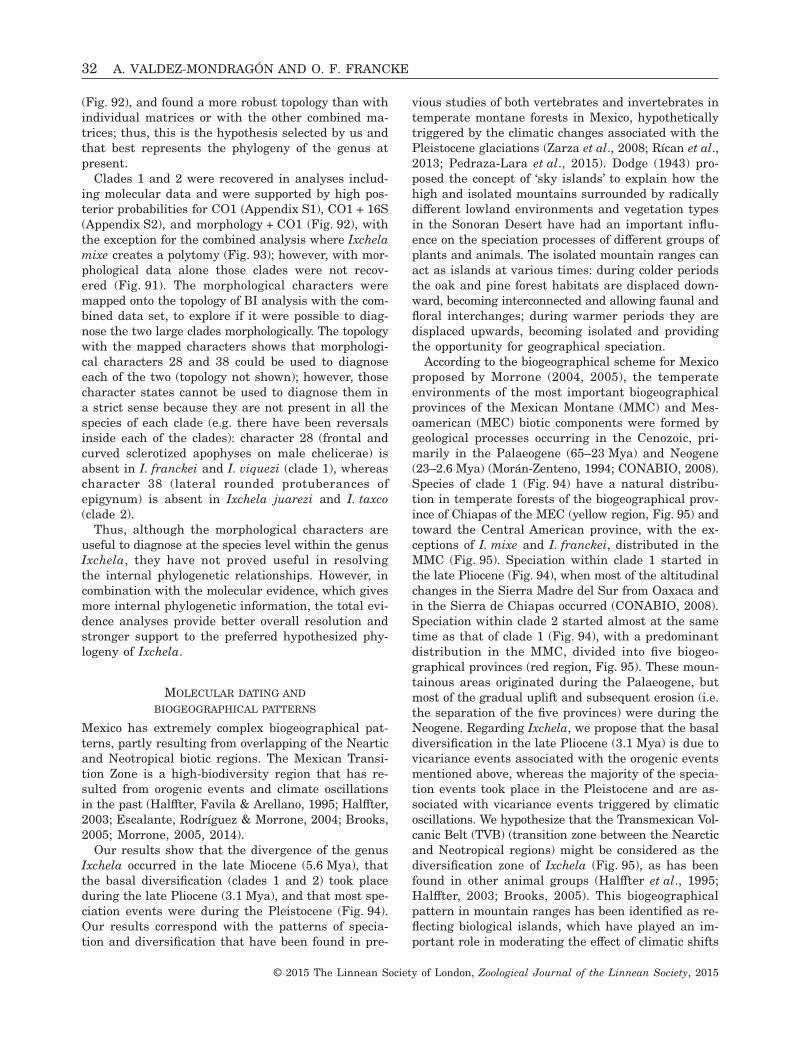
(Fig. 92), and found a more robust topology than withindividual matrices or with the other combined ma-trices; thus, this is the hypothesis selected by us andthat best represents the phylogeny of the genus atpresent.

Clades 1 and 2 were recovered in analyses includ-ing molecular data and were supported by high pos-terior probabilities for CO1 (Appendix S1), CO1 + 16S(Appendix S2), and morphology + CO1 (Fig. 92), withthe exception for the combined analysis where Ixchelamixe creates a polytomy (Fig. 93); however, with mor-phological data alone those clades were not recov-ered (Fig. 91). The morphological characters weremapped onto the topology of BI analysis with the com-bined data set, to explore if it were possible to diag-nose the two large clades morphologically. The topologywith the mapped characters shows that morphologi-cal characters 28 and 38 could be used to diagnoseeach of the two (topology not shown); however, thosecharacter states cannot be used to diagnose them ina strict sense because they are not present in all thespecies of each clade (e.g. there have been reversalsinside each of the clades): character 28 (frontal andcurved sclerotized apophyses on male chelicerae) isabsent in I. franckei and I. viquezi (clade 1), whereascharacter 38 (lateral rounded protuberances ofepigynum) is absent in Ixchela juarezi and I. taxco(clade 2).

Thus, although the morphological characters areuseful to diagnose at the species level within the genusIxchela, they have not proved useful in resolvingthe internal phylogenetic relationships. However, incombination with the molecular evidence, which givesmore internal phylogenetic information, the total evi-dence analyses provide better overall resolution andstronger support to the preferred hypothesized phy-logeny of Ixchela.

MOLECULAR DATING AND

BIOGEOGRAPHICAL PATTERNS

Mexico has extremely complex biogeographical pat-terns, partly resulting from overlapping of the Nearticand Neotropical biotic regions. The Mexican Transi-tion Zone is a high-biodiversity region that has re-sulted from orogenic events and climate oscillationsin the past (Halffter, Favila & Arellano, 1995; Halffter,2003; Escalante, Rodríguez & Morrone, 2004; Brooks,2005; Morrone, 2005, 2014).

Our results show that the divergence of the genusIxchela occurred in the late Miocene (5.6 Mya), thatthe basal diversification (clades 1 and 2) took placeduring the late Pliocene (3.1 Mya), and that most spe-ciation events were during the Pleistocene (Fig. 94).Our results correspond with the patterns of specia-tion and diversification that have been found in pre-

vious studies of both vertebrates and invertebrates intemperate montane forests in Mexico, hypotheticallytriggered by the climatic changes associated with thePleistocene glaciations (Zarza et al., 2008; Rícan et al.,2013; Pedraza-Lara et al., 2015). Dodge (1943) pro-posed the concept of ‘sky islands’ to explain how thehigh and isolated mountains surrounded by radicallydifferent lowland environments and vegetation typesin the Sonoran Desert have had an important influ-ence on the speciation processes of different groups ofplants and animals. The isolated mountain ranges canact as islands at various times: during colder periodsthe oak and pine forest habitats are displaced down-ward, becoming interconnected and allowing faunal andfloral interchanges; during warmer periods they aredisplaced upwards, becoming isolated and providingthe opportunity for geographical speciation.

According to the biogeographical scheme for Mexicoproposed by Morrone (2004, 2005), the temperateenvironments of the most important biogeographicalprovinces of the Mexican Montane (MMC) and Mes-oamerican (MEC) biotic components were formed bygeological processes occurring in the Cenozoic, pri-marily in the Palaeogene (65–23 Mya) and Neogene(23–2.6 Mya) (Morán-Zenteno, 1994; CONABIO, 2008).Species of clade 1 (Fig. 94) have a natural distribu-tion in temperate forests of the biogeographical prov-ince of Chiapas of the MEC (yellow region, Fig. 95) andtoward the Central American province, with the ex-ceptions of I. mixe and I. franckei, distributed in theMMC (Fig. 95). Speciation within clade 1 started inthe late Pliocene (Fig. 94), when most of the altitudinalchanges in the Sierra Madre del Sur from Oaxaca andin the Sierra de Chiapas occurred (CONABIO, 2008).Speciation within clade 2 started almost at the sametime as that of clade 1 (Fig. 94), with a predominantdistribution in the MMC, divided into five biogeo-graphical provinces (red region, Fig. 95). These moun-tainous areas originated during the Palaeogene, butmost of the gradual uplift and subsequent erosion (i.e.the separation of the five provinces) were during theNeogene. Regarding Ixchela, we propose that the basaldiversification in the late Pliocene (3.1 Mya) is due tovicariance events associated with the orogenic eventsmentioned above, whereas the majority of the specia-tion events took place in the Pleistocene and are as-sociated with vicariance events triggered by climaticoscillations. We hypothesize that the Transmexican Vol-canic Belt (TVB) (transition zone between the Nearcticand Neotropical regions) might be considered as thediversification zone of Ixchela (Fig. 95), as has beenfound in other animal groups (Halffter et al., 1995;Halffter, 2003; Brooks, 2005). This biogeographicalpattern in mountain ranges has been identified as re-flecting biological islands, which have played an im-portant role in moderating the effect of climatic shifts



and are responsible for generating biological diversi-fication (Hewitt, 1996; Médail & Quezel, 1997; Médail& Diadema, 2009).

ACKNOWLEDGEMENTS

A.V-M. thanks the Instituto de Biología (IBUNAM),Posgrado en Ciencias Biológicas of UNAM for educa-tion support and the Consejo Nacional de Ciencia yTecnología (CONACYT) for scholarship support duringthe PhD research, and financial support for visits tothe Field Museum of Natural History (FMNH), Chicago,United States, and the Zoologisches ForschungsmuseumAlexander Koenig (ZFMK), Bonn, Germany. A.V-M.thanks the PhD advisory committee members for theirsuggestions and support during the project: Dr AdrianNieto Montes de Oca and Dr David Sebastian Gernandt.

We thank Dr Helga Ochoterena Booth, Dr AlejandroZaldívar Riverón, Dr Juan José Morrone Lupi and DrFernando Álvarez Noguera for their comments and sug-gestions. We thank Berenit Mendoza Gárfias for theSEM photomicrographs, Laura Márquez Valdemar forhelp with sequencing of the genes and Dr CarlosPedraza Lara for his advice on molecular dating. KariMcWest helped with revision of the English text. Specialthanks to the students of the Colección Nacional deArácnidos (CNAN) and the Colección Nacional de Ácaros(CNAC) of Instituto de Biología (IBUNAM) for theirhelp with fieldwork. Our thanks also go to Dr BernhardA. Huber for his constructive comments and sugges-tions, and for hosting the first author at the ZFMK,and to Dr Norman I. Platnick, Dr Javier PonceSaavedra, Dr Carlos Víquez Nuñez, Dr Diana Silva,Dr Petra Sierwald and Mr James Reddell for the loan

Figure 95. Biogeographical provinces of Mexico following the scheme of Morrone (2004, 2005), showing the distributionof the genus Ixchela. Red background colour indicates the Mexican Montane biotic component and its provinces: 1, SierraMadre Occidental (no records of Ixchela); 2, Transmexican Volcanic Belt (species recorded in green); 3, Sierra MadreOriental (species recorded in yellow); 4, Cuenca del Balsas (no records of Ixchela); 5, Sierra Madre del Sur (species rec-orded in dark blue). Yellow background colour indicates the Province of Chiapas (species recorded in light blue) whichbelongs to the Mesoamerican biotic component and is extended toward mountainous zones of Central America (Guate-mala, Honduras, El Salvador and Nicaragua).



and donation of biological material. We extend our ap-preciation to the inhabitants of the different local-ities in Mexico for allowing us to do fieldwork on theirland, and for their assistance with fieldwork. The speci-mens were collected with Scientific Collector PermitFAUT-0175 from the Secretaría de Medio Ambiente yRecursos Naturales (SEMARNAT) to Dr Oscar F.Francke.

REFERENCES

Agnarsson I, Miller JA. 2008. Is ACCTRAN better thanDELTRAN? Cladistics 24: 1032–1038.

Álvarez-Padilla F, Dimitrov D, Giribet G, Hormiga G. 2009.Phylogenetic relationships of the spider family Tetragnathidae(Araneae, Araneoidea) based on morphological and DNA se-quence data. Cladistics 25: 109–146.

Applegate AD. 1999. ArcView GIS version 3.2. Environmen-tal Systems Research Institute, Inc. Neuron Data, Inc.

Arnedo MA, Coddington J, Agnarsson I, Gillespie RG. 2004.From a comb to a tree: phylogenetic relationships of the comb-footed spiders (Araneae, Theridiidae) inferred from nuclearand mitochondrial genes. Molecular Phylogenetic Evolution31: 225–245.

Astrin JJ, Huber BA, Misof B, Klütsch CFC. 2006.Molecular taxonomy in pholcid spiders (Pholcidae: Araneae):evaluation of species identification methods using CO1 and16S and rRNA. Zoologica Scripta 35: 441–457.

Ballard JWO. 1996. Combining data in phylogenetic analy-sis. Trends in Ecology and Evolution 11: 334–335.

Bremer K. 1988. The limits of amino acid sequence data inangiosperm phylogeny reconstruction. Evolution 42: 795–803.

Brooks DR. 2005. Historical biogeography and the age of com-plexity: expansion and integration. Revista Mexicana deBiodiversidad 76: 79–94.

Bruvo-Madaric B, Huber BA, Steinacher A, Pass G. 2005.Phylogeny of Pholcid spiders (Araneae: Pholcidae): com-bined analysis using morphology and molecules. MolecularPhylogenetics and Evolution 37: 661–673.

Cameron SA, Williams PH. 2003. Phylogeny of bumble beesin the new world subgenus Fervidobombus (Hymenoptera:Apidae): congruence of molecular and morphological data. Mo-lecular Phylogenetics and Evolution 28: 552–563.

Coates AG, Jackson JBC, Collins LS, Cronin TM, DowsettHJ, Bybell LM, Jung P, Obando JA. 1992. Closure of theIsthmus of Panama: the near-shore marin record of CostaRica and western Panama. Geological Sociey of America Bul-letin 104: 814–828.

CONABIO. 2008. Capital Natural de México, Vol. I Conocimientoactual de la Biodiversidad. México: Comisión Nacional parael Conocimiento y uso de la Biodiversidad. 1–30.

Dimitrov D, Astrin JJ, Huber BA. 2012. Pholcid spider mo-lecular systematics revisited, with new insights into the bio-geography and the evolution of the group. Cladistics 1: 1–15.

Dodge N. 1943. Monument in the mountain. Arizona High-ways (Phoenix, Arizona: Arizona Highway Department) 19:20–28.

Dorchin N, Freidberg A, Mokady O. 2004. Phylogeny of theBaldratiina (Diptera: Cecidomyiidae) inferred from morpho-logical, ecological and molecular data sources, and evolu-tionary patterns in plant–galler relationships. MolecularPhylogenetics and Evolution 30: 503–515.

Drummond AJ, Xie W, Heled J. 2012. Bayesian inferenceof species trees from multilocus data using BEAST:Bayesian evolutionary analysis by sampling trees. BMC Evo-lutionary Biology 8: 1–18.

Escalante T, Rodríguez G, Morrone JJ. 2004. The diver-sification of Nearctic mammals in the Mexican transition zone.Biological Journal of the Linnean Society 83: 327–339.

Farris JS. 1970. Methods for computing Wagner trees. Sys-tematic Zoology 19: 83–92.

Fitch WM. 1971. Towards defining the course of evolution:minimal change for a specific tree topology. Systematic Zoology20: 406–416.

Folmer M, Black W, Lutz R, Vrijenhoek R. 1994. DNAprimers for amplification of mitochondrial cytochrome c oxidasesubunit I from diverse metazoan invertebrates. MolecularMarine Biology and Biotechnology 3: 294–299.

Gertsch WJ. 1971. A report on some Mexican cave spiders.Bulletin Association for Mexican Cave Studies 4: 47–111.

Goloboff P. 1993. Estimating character weights during treesearch. Cladistics 9: 83–91.

Goloboff P. 1995. Parsimony and weighting: a reply to Turnerand Zandee. Cladistics 11: 91–104.

Goloboff P, Farris JS, Källersjö M, Oxelman B, RamírezMJ, Szumik CA. 2003. Improvements to resampling meas-ures of group support. Cladistics 19: 324–332.

Goloboff P, Farris JS, Nixon KC. 2008. TNT, a free programfor phylogenetic analysis. Cladistics 24: 774–786.

Halffter G. 2003. Biogeografía de montaña de la entomofaunade México y América Central. In: Morrone JJ, Llorente-Bousquets J, eds. Una perspectiva latinoamericana de labiogeografía. México: Las Prensas de Ciencias, UNAM, 87–97.

Halffter G, Favila ME, Arellano L. 1995. Spatial distribu-tion of three groups of Coleoptera along an altitudinal transectin the Mexican Transition Zone and its biogeographical im-plications. Elytron 9: 151–185.

Hall TA. 1999. BioEdit: a user-friendly biological sequence align-ment editor and analysis program for Windows 95/98/NT.Nucleic Acids Symposium Series 41: 95–98.

Hebert PDN, Cywinska A, Ball SL, deWaard JR. 2003a.Biological identifications through DNA barcodes. Proceed-ings of the Royal Society of London. Series B, BiologicalSciences 270: 313–321.

Hebert PDN, Ratnasingham S, deWaard JR. 2003b.Barcoding animal life: cytochrome c oxidase subunit 1 di-vergences among closely related species. Proceedings of theRoyal Society of London. Series B, Biological Sciences 270:596–599.

Hebsgaard MB, Andersen NM, Damgaard J. 2004. Phy-logeny of the true water bugs (Nepomorpha: Hemiptera–Heteroptera) based on 16S and 28S rDNA and morphology.Systematic Entomology 29: 488–508.



Hendrixson BE, DeRyssy BM, Hamilton CA, Bond JE.2013. An exploration of species boundaries in turret-building tarantulas of the Mojave Desert (Araneae,Mygalomorphae, Theraphosidae, Aphonopelma). MolecularPhylogenetics and Evolution 66: 327–340.

Hewitt GM. 1996. Some genetic consequences of ice ages, andtheir role in divergence and speciation. Biological Journalof the Linnean Society 58: 247–276.

Hillis DM, Moritz C, Mable BK. 1996. Molecular systemat-ics, 2nd edn. Sunderland, MA: Sinauer.

Huber BA. 1998a. Report on some pholcid spiders collectedin Guatemala and Honduras (Araneae, Pholcidae). RevueSuisse de Zoologie 105: 49–80.

Huber BA. 1998b. Genital mechanics in some neotropicalpholcid spiders (Araneae: Pholcidae), with implications forsystematics. Journal of Zoology, London 244: 587–599.

Huber BA. 2000. New World Pholcid Spiders (Araneae:Pholcidae): a revision at generic level. Bulletin of the Ameri-can Museum of Natural History 254: 1–348.

Huber BA. 2001. The pholcids of Australia (Araneae; Pholcidae):taxonomy, biogeography, and relationships. Bulletin of theAmerican Museum of Natural History 260: 1–144.

Huber BA. 2011a. Phylogeny and classification of Pholcidae(Araneae): an update. Journal of Arachnology 39: 211–222.

Huber BA. 2011b. Revision and cladistic analysis of Pholcusand closely related taxa (Araneae, Pholcidae). BonnerZoologische Monographien. Herausgeber: ZoologischesPforschungsmuseum Alexander Koenig 58: 1–509.

Huber BA, Astrin JJ. 2009. Increased sampling blurs mor-phological and molecular species limits: revision of theHispaniolan endemic spider genus Tainonia (Araneae:Pholcidae). Invertebrate Systematics 23: 281–300.

Huber BA, Fischer N, Astrin JJ. 2010. High level ofendemism in Haiti’s last remaining forests: a revision ofModisimus (Araneae: Pholcidae) on Hispaniola, using mor-phology and molecules. Zoological Journal of the LinneanSociety 158: 244–299.

Huelsenbeck JP, Bull JJ, Cunningham CW. 1996. Com-bining data in phylogenetic analysis. Trends in Ecology andEvolution 11: 152–158.

Huelsenbeck JP, Crandall KA. 1997. Phylogeny estima-tion and hypothesis testing using maximum likelihood. AnnualReview of Ecology and Systematics 28: 437–466.

Huelsenbeck JP, Ronquist FR. 2001. MrBayes: Bayesianinference of phylogeny. Bioinformatics 17: 754–755.

Iturralde-Vinent MA. 2005. La Paleogeografía del Caribe ysus implicaciones para la biogeografía histórica. Revista delJardín Botánico Nacional 25–26: 49–78.

Katoh K, Toh H. 2008. Recent developments in the MAFFTmultiple sequence alignment program. Briefings inBioinformatics 4: 286–298. MAFFT version 6, Available at:http://mafft.cbrc.jp/alignment/software/

Kluge AG. 1989. A concern for evidence and a phylogenetichypothesis of relationships among Epicrates (Boidae,Serpentes). Systematic Zoology 38: 7–25.

Lanfear R, Calcott B, Ho SYW, Guidon S. 2012.PartitionFinder: combined selection of partitioning schemes

and substitution models for phylogenetic analyses. Molecu-lar Biology and Evolution 29: 1695–1701.

Lanfear R, Calcott B, Kainer D, Mayer C, Stamatakis A.2014. Selecting optimal partitioning schemes for phylogeneticdatasets. BMC Evolutionary Biology 14: 1–82.

Médail F, Diadema K. 2009. Glacial refugia influence plantdiversity patterns in the Mediterranean Basin. Journal ofBiogeography 36: 1333–1345.

Médail F, Quezel P. 1997. Hot-spots analysis for conserva-tion of plant biodiversity in the Mediterranean Basin. Annalsof the Missouri Botanical Garden 84: 112–127.

Morán-Zenteno DJ. 1994. Geology of the Mexican Republic.American Association of Petroleum Geologist, Studies in Geology39: 1–160.

Morrone JJ. 2004. Panbiogeografía, componentes bióticos yzonas de transición. Revista Brasileira de Entomologia 48:149–162.

Morrone JJ. 2005. Hacia una síntesis biogeográfica de México.Revista Mexicana de Biodiversidad 76: 207–252.

Morrone JJ. 2014. Cladistic biogeography of the Neotropicalregion: identifying the main events in the diversification ofthe terrestrial biota. Cladistics 30: 202–214.

Nixon KC. 2004. WinClada–Asado, version 1.7. Computer soft-ware. Available at: http://www.cladistics.com

Pedraza-Lara C, Barrientos-Lozano L, Rocha-Sánchez AY,Zaldívar-Riverón A. 2015. Montane and coastal species di-versification in the economically important Mexicangrasshopper genus Sphenarium (Orthoptera: Pyrgomorphidae).Molecular Phylogenetics and Evolution 84: 220–231.

Pickard-Cambridge FO. 1902. Arachnida.-Araneida andOpiliones. Biologia Centrali-Americana, Zoology, London 2:313–424.

Pickard-Cambridge O. 1898. Arachnida.-Araneida. BiologiaCentrali-Americana, Zoology, London 1: 233–288.

Poinar GO. 1992. Life in amber. Stanford, CA: Stanford Uni-versity Press, 366.

Posada D. 2008. jModelTest: pylogenetic model averaging. Mo-lecular Biology and Evolution 25: 1253–1256.

Posada D, Buckley TR. 2004. Model selection and model av-eraging in phylogenetics: advantages of the AIC and Bayes-ian approaches over likelihood ratio tests. Systematic Biology50: 580–601.

Rambaut A, Drummond AJ. 2002–2013. TreeAnnotator version1.7.5. Edinburgh/Auckland: Institute of Evolutionary Biology,University of Edinburgh; Department of Computer Science,University of Auckland.

Rambaut A, Drummond AJ. 2003–2009. TRACER, MCMCtrace analysis tool version 1.5. Edinburgh/Auckland:Institute of Evolutionary Biology, University of Edinburgh;Department of Computer Science, University of Auckland.

Rícan O, Piálek L, Zardoya R, Doadrio I, Zrzavý J. 2013.Biogeography of the Mesoamerican Cichlidae (Teleostei:Heroini): colonization through the GAARlandia land bridgeand early diversification. Journal of Biogeography 40: 579–593.

Swofford DL, Maddison WP. 1987. Reconstructing ances-tral character states under Wagner parsimony. Mathemati-cal Biosciences 87: 199–229.



http://mafft.cbrc.jp/alignment/software/

http://www.cladistics.com

Valdez-Mondragón A. 2013. Taxonomic revision of the spidergenus Ixchela Huber, 2000 (Araneae: Pholcidae), with de-scription of ten new species from Mexico and Central America.Zootaxa 3608: 285–327.

Wunderlich J. 1988. Die fossilen Spinnen im dominikanischenBernstein. Beiträge zur Araneologie 2: 1–378.

Zarza E, Reynoso VH, Emerson BC. 2008. Diversificationin the northern neotropics: mitochondrial and nuclear DNAphylogeography of the iguana Ctenosaura pectinata and relatedspecies. Molecular Ecology 17: 3259–3275.

APPENDIX 1

Morphological characters used in the phylogenetic analy-sis (40 characters [34 binary and six multistate]) wereas follows:

Palp

1. Male, bulb prolateroventral apophysis (PAB) (Fig. 1):(0) absent, (1) present.

2. Male, femur shape: (0) wide (Physocyclus, Priscula),(1) slender basally, markedly wide in the distal thirdpart (‘Coryssocnemis’), (2) long and slender, withcone-shaped (Figs 38, 49).

3. Embolus, ventral sclerotized line, from bulb to apicalpart (Fig. 60): (0) absent, (1) present.

4. Male, ventrodistal apophysis (VAF) on femur(Figs 60, 72): (0) absent, (1) present.

5. Male, ventrodistal conical protuberance on femur(Ixchela taxco) (Valdez-Mondragón, 2013; fig. 140):(0) absent, (1) present.

6. Embolus, basal protuberance, ending in round tip,near to PAB: (0) absent, (1) present.

7. Embolus, apical ventral projection (Figs 8, 10, 44):(0) absent, (1) present.

8. Embolus, apical dorsal projection, spine-shaped(Figs 2, 39, 50): (0) absent, (1) present.

9. Embolus, ratio: (0) length of embolus < diameterof bulb, (1) length of embolus > diameter ofbulb.

10. Embolus, dorsal thin sclerotized line: (0) absent,embolus without pattern, (1) present.

11. Embolus, dorsal-retrolateral line: (0) absent, emboluswithout pattern, (1) present and sclerotized, longand wide (Figs 38, 49).

12. Procursus, ‘brush’ of pseudotrichia distally: (0)absent, (1) present.

13. Procursus with ventral pocket and dorsal apophysis:(0) absent, (1) present.

14. Tarsus, dorsal apophysis 1b, basally: (0) absent,(1) present in dorsal part, (2) present in retrolateralpart.

15. Tarsus, dorsal apophysis 1d, basally: (0) absent,(1) present in dorsal part, (2) present in retrolateralpart.

16. Procursus, projections on sub-distal part: (0) absent,flat sub-distal part, (1) present, serrated or withsmall poorly sclerotized (Aymaria).

17. Procursus, sclerotized spine distally, smalland curved (Figs 38, 49): (0) absent, (1)present.

18. Procursus, long setae: (0) absent, flat procursus(1) present on ventral-basal part, (2) present onventral protuberance (VPP) (Figs 15, 38, 60).

19. Procursus, basal-dorsal part: (0) without setae, (1)with setae.

20. Procursus, setae on basal-dorsal part, number:(0) two setae (Fig. 14), (1) three setae(Fig. 16).

21. Procursus, shape: (0) short with long and straightspine distally, (1) thin and wide distally (Priscula),(2) conical and long (Ixchela) (Figs 49, 50, 72), (3)conical and wide basally (‘Coryssocnemis’, Aymaria,Huber, 2000; fig. 583).

22. Embolus, ventrally with a small sub-distallysclerotized spine (arrow, Fig. 9): (0) absent, embolusflat, (1) present.

23. Male, coxa with retrolateral apophysis: (0) absent,(1) present.

Chelicerae

24. Male, frontal apophysis of chelicerae (FAC)(Figs 26, 36, 37): (0) absent, FAC flat, (1)present.

25. Male, shape of FAC: (0) short and wide, locatedon median part of chelicerae, (1) wide and rounded(Valdez-Mondragón, 2013; figs 74, 100, 189), (2)conical and small (Valdez-Mondragón, 2013; figs 21,22, 62, 63), (3) conical, long and wide(Valdez-Mondragón, 2013; figs 162, 163), (4) conicaland very small, located near to retrolateral part(Valdez-Mondragón, 2013; figs 149, 204), (5) longand slightly curved, located near to prolateral part(Valdez-Mondragón, 2013; fig. 112), (6) long andcurved, located basally on median part of eachchelicerae (Valdez-Mondragón, 2013; figs 136, 137),(7) small and rounded, located on central part ofchelicerae (Valdez-Mondragón, 2013; figs 124, 125),(8) long and conical, slightly projected toward upand slightly curved apically (Fig. 51).

26. Male, distal-frontal apophysis, next to the fangs(Aymaria): (0) absent, flat region next to the fangs,(1) present.

27. Female, lateral stridulatory files: (0) absent,chelicerae flat, (1) present.

28. Male, frontal-distal sclerotized apophyses (SAC):(0) absent, chelicerae flat, (1) present, reminis-cent (Valdez-Mondragón, 2013; fig. 74), (2) present,highly visible (Figs 26, 27, 37).



29. Chelicerae of male, frontal and curved sclerotizedapophyses (Valdez-Mondragón, 2013; figs 49, 88):(0) absent, (1) present.

Prosoma

30. Carapace, dorsal pattern around the fovea: (0) com-plete, touching the ocular region (Fig. 35), (1) in-complete, leaving a small region without touchingthe ocular region (Valdez-Mondragón, 2013; fig. 99).

Legs

31. Tibiae and metatarsi with curved setae: (0) absent,(1) present.

32. Femora and tibiae with numerous rings: (0) absent,(1) present.

Opisthosoma

33. Epigynum, ratio: (0) wider that long (Figs 64, 76),(1) longer than wide (Valdez-Mondragón, 2013;figs 95, 183).

34. Epigynum, median septum (MSE) in dorsal view(Figs 43, 54): (0) absent, (1) present.

35. Concavities with sac-shape between MSE and poreplates (Figs 54, 65): (0) absent, (1) present.

36. Epigynum, small and circular concavity in frontaldistal part (Fig. 64): (0) absent, (1) present.

37. Epigynum, lateral constraints in anterior part(Valdez-Mondragón, 2013; figs 41, 95, 183): (0)absent, (1) present.

38. Epigynum, lateral rounded protuberances, near tothe epigastric furrow (Figs 53, 64): (0) absent, (1)present.

39. Epigynum, lateral rounded protuberances each side,size: (0) small and curved (Fig. 55), (1) wide androunded (Fig. 67).

40. Epigynum, lateral rounded protuberances each side,position: (0) next to the epigastric furrow (Fig. 41),(1) leaving a space between the protuberances andthe epigastric furrow (Fig. 66).



AP

PE

ND

IX2

Ch

arac

ter

mat

rix

use

din

the

mor

phol

ogic

alph

ylog

enet

ican

alys

is,

com

pris

ing

24ta

xa(2

0in

grou

p,fo

ur

outg

rou

p),

and

40m

orph

olog

ical

char

acte

rs(3

4bi

nar

yan

dsi

xm

ult

ista

te)

12

34

56

78

910

1112

1314

1516

1718

1920

2122

2324

2526

2728

2930

3132

3334

3536

3738

3940

Ph

ysoc

yclu

sd

uge

si0

00

00

–0

01

00

11

00

00

00

–0

00

–0

10

00

01

00

0–

00

0–

–P

risc

ula

bin

gham

ae0

00

10

–0

00

00

10

12

00

00

–1

00

–0

00

00

00

00

0–

00

0–

–A

ymar

iaco

nic

a0

10

10

–0

00

10

00

11

10

01

13

00

–1

00

01

00

00

10

00

0–

–C

orys

socn

emis

ivie

01

11

0–

00

01

10

01

10

01

11

30

0–

01

00

10

00

00

–0

00

––

Ixch

ela

peck

i1

21

10

11

11

11

00

11

01

21

12

10

–0

00

11

00

00

11

00

0–

–Ix

chel

afu

rcu

la1

21

10

11

11

11

00

11

01

21

12

11

20

00

01

00

01

11

01

0–

–Ix

chel

am

ixe

12

10

00

11

11

10

01

10

12

11

21

10

00

01

11

00

11

10

10

––

Ixch

ela

san

tiba

nez

i1

21

10

11

11

11

00

11

01

21

12

11

20

00

11

00

01

10

01

0–

–Ix

chel

ah

uas

teca

12

11

01

11

11

10

01

10

12

11

21

11

00

10

10

00

01

10

01

00

Ixch

ela

sim

oni

12

11

01

11

11

10

01

10

12

11

21

11

00

10

10

00

01

10

01

00

Ixch

ela

hu

beri

12

11

01

11

11

10

01

10

12

11

21

11

00

00

11

00

01

10

01

00

Ixch

ela

grix

12

11

01

11

11

10

01

10

12

11

21

17

00

00

11

00

01

10

01

00

Ixch

ela

jali

sco

sp.n

ov.

12

11

01

11

11

10

01

10

12

10

21

18

00

20

10

00

01

11

01

00

Ixch

ela

azt

eca

sp.n

ov.

12

11

01

11

11

10

01

10

12

11

21

12

00

20

10

00

01

11

01

00

Ixch

ela

pu

rep

ech

asp

.nov

.1

21

10

11

11

11

00

11

01

21

12

11

20

02

01

00

00

11

10

11

1Ix

chel

afr

anck

ei1

21

10

11

11

11

00

11

01

21

12

11

40

02

01

00

00

10

10

0–

–Ix

chel

ata

xco

12

11

11

11

11

10

01

10

12

11

21

16

00

20

11

00

01

11

00

––

Ixch

ela

juar

ezi

12

11

00

11

11

10

01

10

12

11

21

15

00

10

11

00

01

10

00

––

Ixch

ela

viqu

ezi

12

11

00

11

11

10

01

10

12

11

21

14

00

20

11

00

01

01

00

––

Ixch

ela

plac

ida

12

11

01

11

11

10

01

10

12

11

21

12

00

20

10

00

01

11

01

11

Ixch

ela

tzot

zil

12

11

01

11

11

10

01

10

12

11

21

13

00

10

10

01

01

10

01

11

Ixch

ela

tla

yud

asp

.nov

.1

21

10

11

11

11

00

11

01

21

12

11

20

02

01

00

10

11

10

11

1Ix

chel

aab

ern

ath

yi1

21

10

11

11

11

00

11

01

21

12

11

20

02

01

00

10

11

10

11

1Ix

chel

am

end

oza

isp

.nov

.1

21

10

11

11

11

00

11

01

21

12

11

20

02

01

00

10

11

10

11

1



SUPPORTING INFORMATION

Additional Supporting Information may be found in the online version of this article at the publisher’s web-site:

Appendix S1. Majority consensus tree derived from the Bayesian analysis using the CO1 data set. Numbersabove branches indicate posterior probabilities. Numbers below branches: (+) indicates clades found with PA/Jackknife support values, followed by PA/Bremer support values. Black squares below branches indicate cladesrecovered with PA using different concavity values (K) using implied weighting; white squares indicate cladesnot recovered with some concavity values (see inset). Numbers and arrows indicate clades that are discussedin the text.Appendix S2. Majority consensus tree derived from the Bayesian analysis using the CO1 + 16S data set. Numbersabove branches indicate posterior probabilities. Numbers below branches: (+) indicates clades found with PA/Jackknife support values, followed with PA/Bremer support values. Black squares below branches indicate cladesfound with PA using different concavity values (K) using implied weighting; white squares indicate clades notrecovered with some concavity values (see inset). Numbers and arrows indicate clades that are discussed inthe text.



Valdez-Mondragón, A. & O. F. Francke. 2015. Phylogeny of the spider genus Ixchela Huber, 2000...

Documents

Transcript of Valdez-Mondragón, A. & O. F. Francke. 2015. Phylogeny of the spider genus Ixchela Huber, 2000...