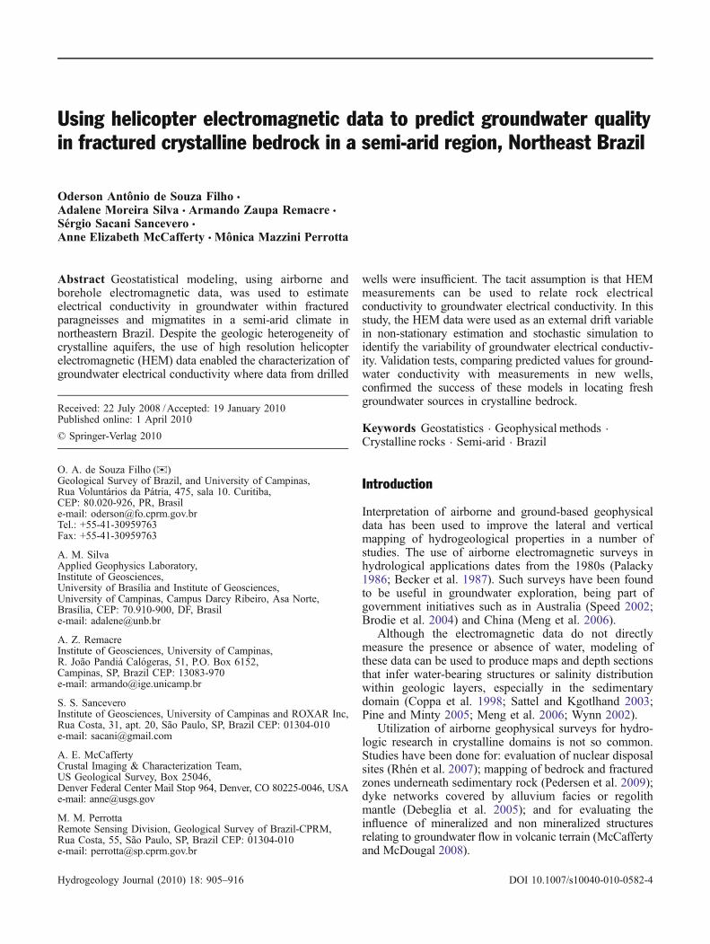
Using helicopter electromagnetic data to predict groundwater qualityin fractured crystalline bedrock in a semi-arid region, Northeast Brazil

Oderson Antônio de Souza Filho &

Adalene Moreira Silva & Armando Zaupa Remacre &

Sérgio Sacani Sancevero &

Anne Elizabeth McCafferty & Mônica Mazzini Perrotta

Abstract Geostatistical modeling, using airborne andborehole electromagnetic data, was used to estimateelectrical conductivity in groundwater within fracturedparagneisses and migmatites in a semi-arid climate innortheastern Brazil. Despite the geologic heterogeneity ofcrystalline aquifers, the use of high resolution helicopterelectromagnetic (HEM) data enabled the characterization ofgroundwater electrical conductivity where data from drilled

wells were insufficient. The tacit assumption is that HEMmeasurements can be used to relate rock electricalconductivity to groundwater electrical conductivity. In thisstudy, the HEM data were used as an external drift variablein non-stationary estimation and stochastic simulation toidentify the variability of groundwater electrical conductiv-ity. Validation tests, comparing predicted values for ground-water conductivity with measurements in new wells,confirmed the success of these models in locating freshgroundwater sources in crystalline bedrock.

Keywords Geostatistics . Geophysical methods .Crystalline rocks . Semi-arid . Brazil

Introduction

Interpretation of airborne and ground-based geophysicaldata has been used to improve the lateral and verticalmapping of hydrogeological properties in a number ofstudies. The use of airborne electromagnetic surveys inhydrological applications dates from the 1980s (Palacky1986; Becker et al. 1987). Such surveys have been foundto be useful in groundwater exploration, being part ofgovernment initiatives such as in Australia (Speed 2002;Brodie et al. 2004) and China (Meng et al. 2006).

Although the electromagnetic data do not directlymeasure the presence or absence of water, modeling ofthese data can be used to produce maps and depth sectionsthat infer water-bearing structures or salinity distributionwithin geologic layers, especially in the sedimentarydomain (Coppa et al. 1998; Sattel and Kgotlhand 2003;Pine and Minty 2005; Meng et al. 2006; Wynn 2002).

Utilization of airborne geophysical surveys for hydro-logic research in crystalline domains is not so common.Studies have been done for: evaluation of nuclear disposalsites (Rhén et al. 2007); mapping of bedrock and fracturedzones underneath sedimentary rock (Pedersen et al. 2009);dyke networks covered by alluvium facies or regolithmantle (Debeglia et al. 2005); and for evaluating theinfluence of mineralized and non mineralized structuresrelating to groundwater flow in volcanic terrain (McCaffertyand McDougal 2008).

Received: 22 July 2008 /Accepted: 19 January 2010Published online: 1 April 2010

* Springer-Verlag 2010

O. A. de Souza Filho ())Geological Survey of Brazil, and University of Campinas,Rua Voluntários da Pátria, 475, sala 10. Curitiba,CEP: 80.020-926, PR, Brasile-mail: oderson@fo.cprm.gov.brTel.: +55-41-30959763Fax: +55-41-30959763

A. M. SilvaApplied Geophysics Laboratory,Institute of Geosciences,University of Brasília and Institute of Geosciences,University of Campinas, Campus Darcy Ribeiro, Asa Norte,Brasília, CEP: 70.910-900, DF, Brasile-mail: adalene@unb.br

A. Z. RemacreInstitute of Geosciences, University of Campinas,R. João Pandiá Calógeras, 51, P.O. Box 6152,Campinas, SP, Brazil CEP: 13083-970e-mail: armando@ige.unicamp.br

S. S. SanceveroInstitute of Geosciences, University of Campinas and ROXAR Inc,Rua Costa, 31, apt. 20, São Paulo, SP, Brazil CEP: 01304-010e-mail: sacani@gmail.com

A. E. McCaffertyCrustal Imaging & Characterization Team,US Geological Survey, Box 25046,Denver Federal Center Mail Stop 964, Denver, CO 80225-0046, USAe-mail: anne@usgs.gov

M. M. PerrottaRemote Sensing Division, Geological Survey of Brazil-CPRM,Rua Costa, 55, São Paulo, SP, Brazil CEP: 01304-010e-mail: perrotta@sp.cprm.gov.br

Hydrogeology Journal (2010) 18: 905–916 DOI 10.1007/s10040-010-0582-4

The Brazilian government has chosen ground-basedgeophysical surveys because of the lower costs to coversmall areas. The usefulness of airborne geophysics hasonly recently been evaluated for water resource applica-tions in crystalline regions of Brazil. Silva (2005) studiedthe time-domain electromagnetic data and magnetic datain a semi-arid region of Bahia State (south of the studyarea). Souza Filho et al. (2007a,b) have processed andintegrated airborne geophysical (magnetic and electro-magnetic), remote sensing and geologic data usingBayesian analysis to create favorability maps in the samestudy area of this publication, and so did Mandrucci et al.(2008) with data sets for part of São Paulo State.

The integration of sparse borehole data and geo-physical data is very common as discussed in Chamberset al. (2000), Rubin and Hubbard (2005) and in Gómez-Hernández (2005), and also necessary when the hetero-geneity of a hydrogeologic parameter is known. Theborehole data provide direct information about hydro-geological properties with depth at a single location andnon-invasive geophysical techniques enable a more laterallycontinuous mapping. The result of this combination is abetter prediction of hydrogeologic properties at a locationand the possibility to extrapolate such information awayfrom the borehole with a certain confidence level.

In 2001, a high-resolution helicopter electromagnetic(HEM) andmagnetic survey (Lasa Engenharia e ProspecçõesS/A 2001) was carried out in a small area of Northeast Brazil.It was the first airborne survey designed for hydrogeologicalresearch in Brazil (PROASNE 2007). Detailed geologicalmapping and water quality data were also collected fromwater wells in the surveyed area (Souza Filho 1998; SouzaFilho et al. 2003; Veríssimo and Feitosa 2002).

The high variability of water electrical conductivity isvery well known in the crystalline rocks of Brazil’s semi-arid region (Silva et al. 2001; Manoel Filho 1996; Sousaet al. 1984). This study introduces the use of geostatistical

methods together with more-dense airborne geophysicaldata to improve the determination of spatial distribution ofgroundwater electrical conductivity (and therefore inferwater quality) and its heterogeneity within saline water-bearing fractures. The apparent electrical conductivitycalculated from HEM data was used as external variableto characterize the variability of groundwater electricalconductivity. Two techniques were chosen to compare theresults of integrating an external variable function into adeterministic approach (kriging technique) and variabilityestimation (sequential Gaussian simulation technique).

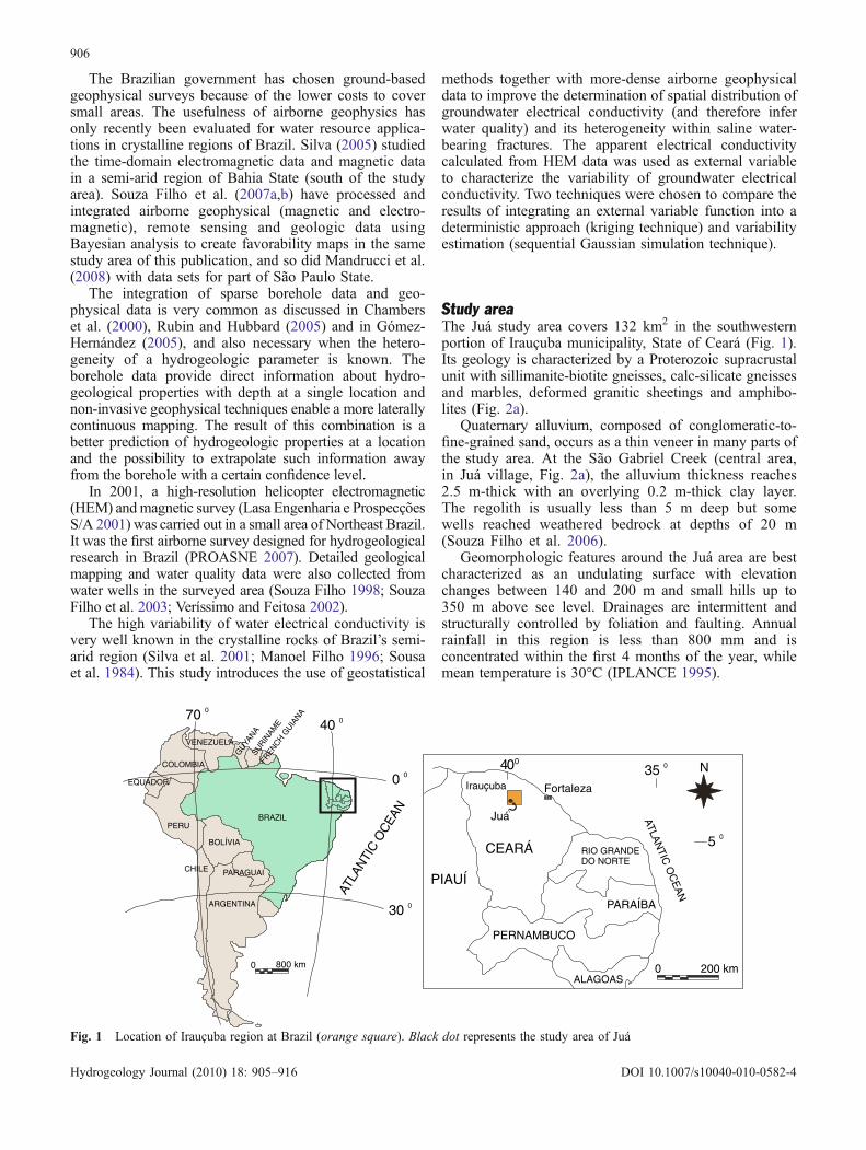
Study areaThe Juá study area covers 132 km2 in the southwesternportion of Irauçuba municipality, State of Ceará (Fig. 1).Its geology is characterized by a Proterozoic supracrustalunit with sillimanite-biotite gneisses, calc-silicate gneissesand marbles, deformed granitic sheetings and amphibo-lites (Fig. 2a).

Quaternary alluvium, composed of conglomeratic-to-fine-grained sand, occurs as a thin veneer in many parts ofthe study area. At the São Gabriel Creek (central area,in Juá village, Fig. 2a), the alluvium thickness reaches2.5 m-thick with an overlying 0.2 m-thick clay layer.The regolith is usually less than 5 m deep but somewells reached weathered bedrock at depths of 20 m(Souza Filho et al. 2006).

Geomorphologic features around the Juá area are bestcharacterized as an undulating surface with elevationchanges between 140 and 200 m and small hills up to350 m above see level. Drainages are intermittent andstructurally controlled by foliation and faulting. Annualrainfall in this region is less than 800 mm and isconcentrated within the first 4 months of the year, whilemean temperature is 30°C (IPLANCE 1995).

70 0

40 0

ATLA

NTI

CO

CEA

N

0 0

VENEZUELA

COLOMBIA

EQUADOR

PERU

BOLÍVIA

CHILE PARAGUAI

ARGENTINA

BRAZIL

GUYA

NASU

RINAM

E

FREN

CHG

UIANA

0 800 km

30 0

200 km0

400

CEARÁ

PIAUÍ

RIO GRANDEDO NORTE

PARAÍBA

PERNAMBUCO

Fortaleza

Juá

Irauçuba35 0

5 0

ALAGOAS

N

ATLAN

TICO

CE

AN

Fig. 1 Location of Irauçuba region at Brazil (orange square). Black dot represents the study area of Juá

906

Hydrogeology Journal (2010) 18: 905–916 DOI 10.1007/s10040-010-0582-4

Most of the people in the study area work and live infarms; they cultivate corn and beans, and raise goats andcattle for their own use. Those who live in Juá village areprovided with water through a public system consisting of

two drilled wells; one for domestic use and anotherconnected to a desalination system that provides potablewater for cooking and drinking. Outside the village,inhabitants get their water from drilled wells and

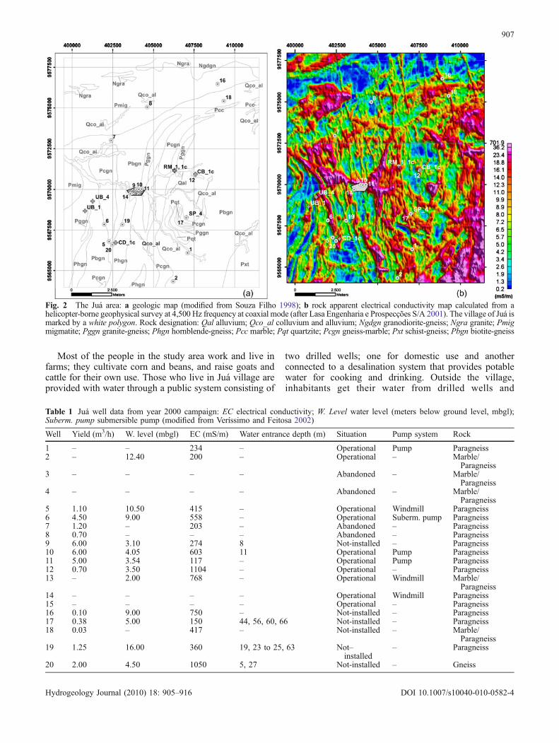
Fig. 2 The Juá area: a geologic map (modified from Souza Filho 1998); b rock apparent electrical conductivity map calculated from ahelicopter-borne geophysical survey at 4,500 Hz frequency at coaxial mode (after Lasa Engenharia e Prospecções S/A 2001). The village of Juá ismarked by a white polygon. Rock designation: Qal alluvium; Qco_al colluvium and alluvium; Ngdgn granodiorite-gneiss; Ngra granite; Pmigmigmatite; Pggn granite-gneiss; Phgn hornblende-gneiss; Pcc marble; Pqt quartzite; Pcgn gneiss-marble; Pxt schist-gneiss; Pbgn biotite-gneiss

Table 1 Juá well data from year 2000 campaign: EC electrical conductivity; W. Level water level (meters below ground level, mbgl);Suberm. pump submersible pump (modified from Veríssimo and Feitosa 2002)

Well Yield (m3/h) W. level (mbgl) EC (mS/m) Water entrance depth (m) Situation Pump system Rock

1 – – 234 – Operational Pump Paragneiss2 – 12.40 200 – Operational – Marble/

Paragneiss3 – – – – Abandoned – Marble/

Paragneiss4 – – – – Abandoned – Marble/

Paragneiss5 1.10 10.50 415 – Operational Windmill Paragneiss6 4.50 9.00 558 – Operational Suberm. pump Paragneiss7 1.20 – 203 – Abandoned – Paragneiss8 0.70 – – – Abandoned – Paragneiss9 6.00 3.10 274 8 Not-installed – Paragneiss10 6.00 4.05 603 11 Operational Pump Paragneiss11 5.00 3.54 117 – Operational Pump Paragneiss12 0.70 3.50 1104 – Operational – Paragneiss13 – 2.00 768 – Operational Windmill Marble/

Paragneiss14 – – – – Operational Windmill Paragneiss15 – – – – Operational – Paragneiss16 0.10 9.00 750 – Not-installed – Paragneiss17 0.38 5.00 150 44, 56, 60, 66 Not-installed – Paragneiss18 0.03 – 417 – Not-installed – Marble/

Paragneiss19 1.25 16.00 360 19, 23 to 25, 63 Not–

installed– Paragneiss

20 2.00 4.50 1050 5, 27 Not-installed – Gneiss

907

Hydrogeology Journal (2010) 18: 905–916 DOI 10.1007/s10040-010-0582-4

secondarily by dug wells and small reservoirs. The waterprovided by the wells and reservoirs is typically insuffi-cient to support both human and animal consumption dueto low yields and brackish nature. Such surface andgroundwater deficiencies restrain any economic improve-ments related to agricultural production or cattle ranching.

Data sets

The data sets used in this study comprise electricalconductivity information obtained from the HEM surveyand measurements from water wells. All data wereprojected to a common datum using a Universal Trans-verse Mercator-UTM, zone 24, projection and a SouthAmerican Datum of 1969.

Electrical conductivity (EC) characterizes the ability ofan electric current to be transmitted through a substance.In water, the transmission of a current is due to the polarstructure of water molecules and the interaction withdissolved salts that promote the current movement. Freshand non-fractured rocks are typically electrically resistiveby nature, due to the low electron mobility of main rock-forming minerals. Igneous and metamorphic rocks arevery common in northeastern Brazil and because of largeamounts of quartz and feldspar, they are generally veryelectrically resistive. Therefore, the main factors toincrease bulk rock conductivity are the presence of water,clay minerals, moisture, sulfides or graphite within therock structure (see Telford et al. 1984 and Palacky 1991for a review of electrical properties of minerals andcomparative values for different rocks and minerals in thepresence of water).

Both water EC measurements (µS/cm) and HEM data(mS/m) are provided in units of electrical conductance perdistance, relating to their ability to conduct electric current.Consequently, the water EC was transformed to the sameunit system (mS/m) as the HEM data to better relate theairborne measurements to the water measurements.

Water well dataAqueous electrical conductivity (EC) in groundwater isthe primary variable in this study. The EC was measuredat fifteen of the twenty drilled wells in the Juá area(Fig. 2b; Table 1) during the dry period of November

2000. For validation, during the dry season of November2005, other measurements were taken in these same wells,plus three new wells, two non-operational wells and fourdug wells (Fig. 2a; Table 2). The water EC measurementwas done with a portable conductivity meter. The waterEC was measured either from samples collected from thenon-operational wells or measured directly from waterfrom the pipe that comes out of the productive wells.Water temperatures were between 27 and 31°C. Theconductivity meter was calibrated daily.

Electrical conductivity analysis in drilled wellsLocations of wells in the study area with groundwaterelectrical conductivities measured in the year 2000(Fig. 2a) show a NE–SW trend in map view with higherdensity of wells located near the center part of the studyarea. These data reveal a high anomalous EC value(greater than 1,000 mS/m), which is attributed to highconcentrations of dissolved solids during the dry season.Silva et al. (2001) and Veríssimo and Feitosa (2002)describe the high seasonal variability of water electricalconductivity observed in wells and reservoirs since 1999.EC values can increase up to a factor of three in the dryseason (Table 3) and salinity often follows that behavior.

Electrical conductivity measurements from 2000(Fig. 3) have an approximately log-normal distribution,in which 40% of the samples have EC values greater than100 mS/m and less than 250 mS/m. Other studies also showa similar log normal distribution of EC data for the Irauçubaarea (Veríssimo and Feitosa 2002; Souza Filho et al. 2004)and for other crystalline regions in northeastern Brazil(Manoel Filho 1996).

How EC varies with depth is unknown because of lackof data. Only three wells have EC with depth availablefrom drilling reports. That said, there is a tendency forelectrical conductivity to decrease with depth within thosefew wells (Table 4).

Table 2 Juá well data from 2005 campaign: W. Level water level (meters below ground level, mbgl); EC electrical conductivity (mS/m)

Well Yield (m3/h) W. level (mbgl) EC (mS/m) Situation Pump system Rock

RM_1/drilled 1.5 4.70 184.0 Deactivated Pump ParagneissUB_1/drilled 0.3 12.31 858.0 Non operational Not installed ParagneissUB_4/drilled <0.3 5.73 810.0 Not-installed Operational Not installed Marble/gneissJ_1/drilled <0.3 6.43 290.0 Abandoned Windmill ParagneissSL_4/ drilled <0.3 13.15 321.0 Abandoned Not installed ParagneissSP_4/drilled <0.5 – 151.2 Operational Windmill ParagneissCD_1c/dug – 7.70 261.0 Operational Manual Gneiss/migmatiteCB_1c/dug – – 231.0 Operational Manual ParagneissRM_1c/dug – 3.7 140.4 Operational Manual ParagneissSP_2/drilled <0.5 4.00 219.0 Operational Manual Gneiss/amphibolite

Table 3 Groundwater electrical conductivity measured for wells 10and 11 during the period of 1997–2002. (Silva et al. 2001). Rel.increase relative increase

Well Min. EC (mS/m) Max. EC (mS/m) Rel. increase (%)

10 112.6 375.0 33411 376.0 116.0 324

908

Hydrogeology Journal (2010) 18: 905–916 DOI 10.1007/s10040-010-0582-4

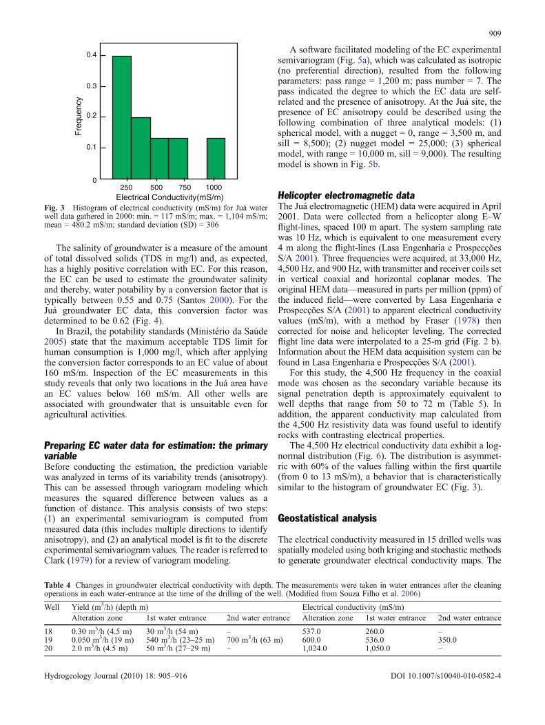
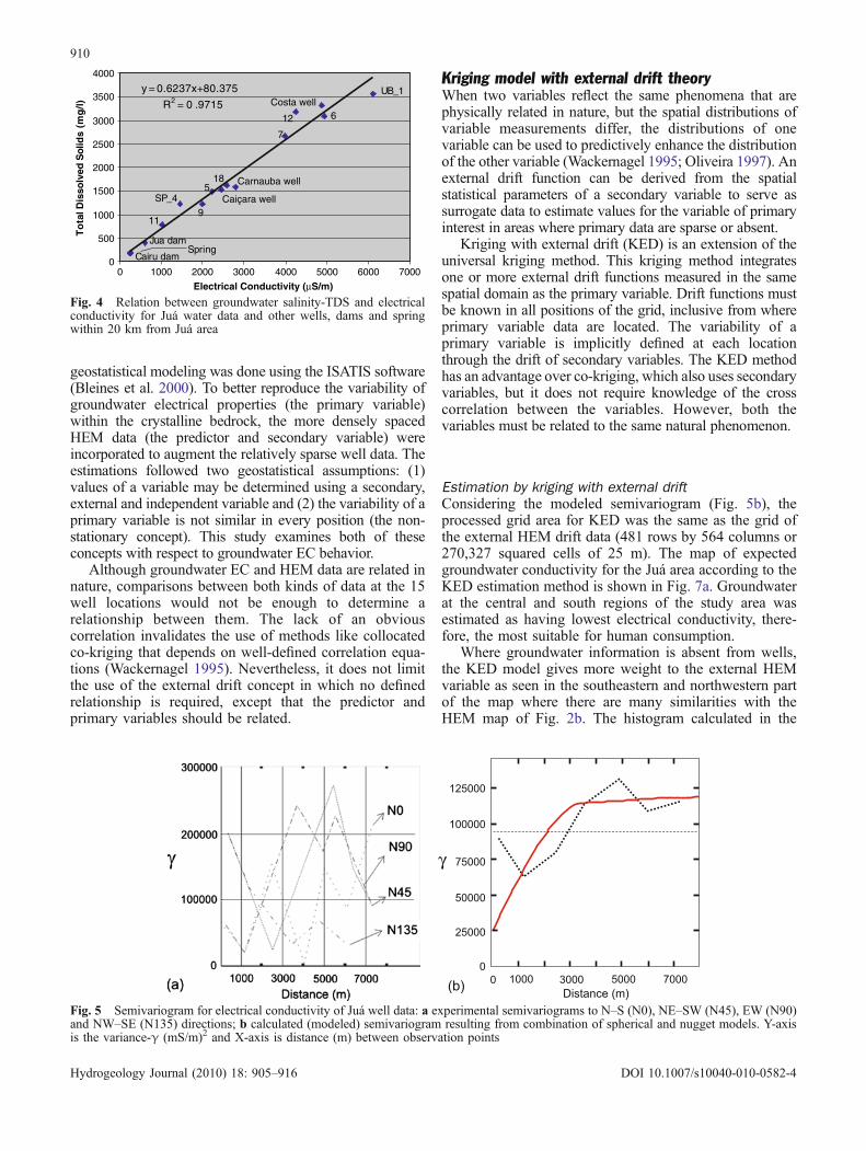
The salinity of groundwater is a measure of the amountof total dissolved solids (TDS in mg/l) and, as expected,has a highly positive correlation with EC. For this reason,the EC can be used to estimate the groundwater salinityand thereby, water potability by a conversion factor that istypically between 0.55 and 0.75 (Santos 2000). For theJuá groundwater EC data, this conversion factor wasdetermined to be 0.62 (Fig. 4).

In Brazil, the potability standards (Ministério da Saúde2005) state that the maximum acceptable TDS limit forhuman consumption is 1,000 mg/l, which after applyingthe conversion factor corresponds to an EC value of about160 mS/m. Inspection of the EC measurements in thisstudy reveals that only two locations in the Juá area havean EC values below 160 mS/m. All other wells areassociated with groundwater that is unsuitable even foragricultural activities.

Preparing EC water data for estimation: the primaryvariableBefore conducting the estimation, the prediction variablewas analyzed in terms of its variability trends (anisotropy).This can be assessed through variogram modeling whichmeasures the squared difference between values as afunction of distance. This analysis consists of two steps:(1) an experimental semivariogram is computed frommeasured data (this includes multiple directions to identifyanisotropy), and (2) an analytical model is fit to the discreteexperimental semivariogram values. The reader is referred toClark (1979) for a review of variogram modeling.

A software facilitated modeling of the EC experimentalsemivariogram (Fig. 5a), which was calculated as isotropic(no preferential direction), resulted from the followingparameters: pass range = 1,200 m; pass number = 7. Thepass indicated the degree to which the EC data are self-related and the presence of anisotropy. At the Juá site, thepresence of EC anisotropy could be described using thefollowing combination of three analytical models: (1)spherical model, with a nugget = 0, range = 3,500 m, andsill = 8,500); (2) nugget model = 25,000; (3) sphericalmodel, with range = 10,000 m, sill = 9,000). The resultingmodel is shown in Fig. 5b.

Helicopter electromagnetic dataThe Juá electromagnetic (HEM) data were acquired in April2001. Data were collected from a helicopter along E–Wflight-lines, spaced 100 m apart. The system sampling ratewas 10 Hz, which is equivalent to one measurement every4 m along the flight-lines (Lasa Engenharia e ProspecçõesS/A 2001). Three frequencies were acquired, at 33,000 Hz,4,500 Hz, and 900 Hz, with transmitter and receiver coils setin vertical coaxial and horizontal coplanar modes. Theoriginal HEM data—measured in parts per million (ppm) ofthe induced field—were converted by Lasa Engenharia eProspecções S/A (2001) to apparent electrical conductivityvalues (mS/m), with a method by Fraser (1978) thencorrected for noise and helicopter leveling. The correctedflight line data were interpolated to a 25-m grid (Fig. 2 b).Information about the HEM data acquisition system can befound in Lasa Engenharia e Prospecções S/A (2001).

For this study, the 4,500 Hz frequency in the coaxialmode was chosen as the secondary variable because itssignal penetration depth is approximately equivalent towell depths that range from 50 to 72 m (Table 5). Inaddition, the apparent conductivity map calculated fromthe 4,500 Hz resistivity data was found useful to identifyrocks with contrasting electrical properties.

The 4,500 Hz electrical conductivity data exhibit a log-normal distribution (Fig. 6). The distribution is asymmet-ric with 60% of the values falling within the first quartile(from 0 to 13 mS/m), a behavior that is characteristicallysimilar to the histogram of groundwater EC (Fig. 3).

Geostatistical analysis

The electrical conductivity measured in 15 drilled wells wasspatially modeled using both kriging and stochastic methodsto generate groundwater electrical conductivity maps. The

0

0.3

Electrical Conductivity(mS/m)250

Fre

quen

cy

0.1

0.2

0.4

500 750 1000

Fig. 3 Histogram of electrical conductivity (mS/m) for Juá waterwell data gathered in 2000: min. = 117 mS/m; max. = 1,104 mS/m;mean = 480.2 mS/m; standard deviation (SD) = 306

Table 4 Changes in groundwater electrical conductivity with depth. The measurements were taken in water entrances after the cleaningoperations in each water-entrance at the time of the drilling of the well. (Modified from Souza Filho et al. 2006)

Well Yield (m3/h) (depth m) Electrical conductivity (mS/m)Alteration zone 1st water entrance 2nd water entrance Alteration zone 1st water entrance 2nd water entrance

18 0.30 m3/h (4.5 m) 30 m3/h (54 m) – 537.0 260.0 –19 0.050 m3/h (19 m) 540 m3/h (23–25 m) 700 m3/h (63 m) 600.0 536.0 350.020 2.0 m3/h (4.5 m) 50 m3/h (27–29 m) – 1,024.0 1,050.0 –

909

Hydrogeology Journal (2010) 18: 905–916 DOI 10.1007/s10040-010-0582-4

geostatistical modeling was done using the ISATIS software(Bleines et al. 2000). To better reproduce the variability ofgroundwater electrical properties (the primary variable)within the crystalline bedrock, the more densely spacedHEM data (the predictor and secondary variable) wereincorporated to augment the relatively sparse well data. Theestimations followed two geostatistical assumptions: (1)values of a variable may be determined using a secondary,external and independent variable and (2) the variability of aprimary variable is not similar in every position (the non-stationary concept). This study examines both of theseconcepts with respect to groundwater EC behavior.

Although groundwater EC and HEM data are related innature, comparisons between both kinds of data at the 15well locations would not be enough to determine arelationship between them. The lack of an obviouscorrelation invalidates the use of methods like collocatedco-kriging that depends on well-defined correlation equa-tions (Wackernagel 1995). Nevertheless, it does not limitthe use of the external drift concept in which no definedrelationship is required, except that the predictor andprimary variables should be related.

Kriging model with external drift theoryWhen two variables reflect the same phenomena that arephysically related in nature, but the spatial distributions ofvariable measurements differ, the distributions of onevariable can be used to predictively enhance the distributionof the other variable (Wackernagel 1995; Oliveira 1997). Anexternal drift function can be derived from the spatialstatistical parameters of a secondary variable to serve assurrogate data to estimate values for the variable of primaryinterest in areas where primary data are sparse or absent.

Kriging with external drift (KED) is an extension of theuniversal kriging method. This kriging method integratesone or more external drift functions measured in the samespatial domain as the primary variable. Drift functions mustbe known in all positions of the grid, inclusive from whereprimary variable data are located. The variability of aprimary variable is implicitly defined at each locationthrough the drift of secondary variables. The KED methodhas an advantage over co-kriging, which also uses secondaryvariables, but it does not require knowledge of the crosscorrelation between the variables. However, both thevariables must be related to the same natural phenomenon.

Estimation by kriging with external driftConsidering the modeled semivariogram (Fig. 5b), theprocessed grid area for KED was the same as the grid ofthe external HEM drift data (481 rows by 564 columns or270,327 squared cells of 25 m). The map of expectedgroundwater conductivity for the Juá area according to theKED estimation method is shown in Fig. 7a. Groundwaterat the central and south regions of the study area wasestimated as having lowest electrical conductivity, there-fore, the most suitable for human consumption.

Where groundwater information is absent from wells,the KED model gives more weight to the external HEMvariable as seen in the southeastern and northwestern partof the map where there are many similarities with theHEM map of Fig. 2b. The histogram calculated in the

Jua dam

Cairu damSpring

11

SP_4

9

5Caiçara well

18 Carnauba well

7

12 6Costa well

UB_1y = 0.6237x+80.375

R2 = 0 .9715

0

500

1000

1500

2000

2500

3000

3500

4000

0 1000 2000 3000 4000 5000 6000 7000

Electrical Conductivity (μS/m)

To

tal D

isso

lved

Sol

ids

(mg

/l)

Fig. 4 Relation between groundwater salinity-TDS and electricalconductivity for Juá water data and other wells, dams and springwithin 20 km from Juá area

Distance (m)

100000

125000

0

0

75000

1000 3000 5000 7000

50000

25000

γ

(b)

Fig. 5 Semivariogram for electrical conductivity of Juá well data: a experimental semivariograms to N–S (N0), NE–SW (N45), EW (N90)and NW–SE (N135) directions; b calculated (modeled) semivariogram resulting from combination of spherical and nugget models. Y-axisis the variance-γ (mS/m)2 and X-axis is distance (m) between observation points

910

Hydrogeology Journal (2010) 18: 905–916 DOI 10.1007/s10040-010-0582-4

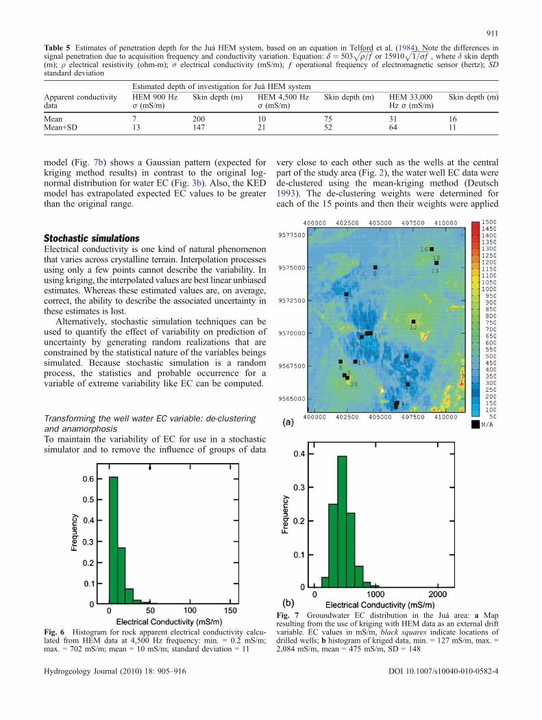
model (Fig. 7b) shows a Gaussian pattern (expected forkriging method results) in contrast to the original log-normal distribution for water EC (Fig. 3b). Also, the KEDmodel has extrapolated expected EC values to be greaterthan the original range.

Stochastic simulationsElectrical conductivity is one kind of natural phenomenonthat varies across crystalline terrain. Interpolation processesusing only a few points cannot describe the variability. Inusing kriging, the interpolated values are best linear unbiasedestimates. Whereas these estimated values are, on average,correct, the ability to describe the associated uncertainty inthese estimates is lost.

Alternatively, stochastic simulation techniques can beused to quantify the effect of variability on prediction ofuncertainty by generating random realizations that areconstrained by the statistical nature of the variables beingssimulated. Because stochastic simulation is a randomprocess, the statistics and probable occurrence for avariable of extreme variability like EC can be computed.

Transforming the well water EC variable: de-clusteringand anamorphosisTo maintain the variability of EC for use in a stochasticsimulator and to remove the influence of groups of data

very close to each other such as the wells at the centralpart of the study area (Fig. 2), the water well EC data werede-clustered using the mean-kriging method (Deutsch1993). The de-clustering weights were determined foreach of the 15 points and then their weights were applied

Table 5 Estimates of penetration depth for the Juá HEM system, based on an equation in Telford et al. (1984). Note the differences insignal penetration due to acquisition frequency and conductivity variation. Equation: d ¼ 503

ffiffiffiffiffiffiffiffi

r=fp

or 15910ffiffiffiffiffiffiffiffiffiffi

1=sfp

, where δ skin depth(m); ρ electrical resistivity (ohm-m); σ electrical conductivity (mS/m); ƒ operational frequency of electromagnetic sensor (hertz); SDstandard deviation

Estimated depth of investigation for Juá HEM systemApparent conductivitydata

HEM 900 Hzσ (mS/m)

Skin depth (m) HEM 4,500 Hzσ (mS/m)

Skin depth (m) HEM 33,000Hz σ (mS/m)

Skin depth (m)

Mean 7 200 10 75 31 16Mean+SD 13 147 21 52 64 11

Fig. 6 Histogram for rock apparent electrical conductivity calcu-lated from HEM data at 4,500 Hz frequency: min. = 0.2 mS/m;max. = 702 mS/m; mean = 10 mS/m; standard deviation = 11

Fig. 7 Groundwater EC distribution in the Juá area: a Mapresulting from the use of kriging with HEM data as an external driftvariable. EC values in mS/m, black squares indicate locations ofdrilled wells; b histogram of kriged data, min. = 127 mS/m, max. =2,084 mS/m, mean = 475 mS/m, SD = 148

911

Hydrogeology Journal (2010) 18: 905–916 DOI 10.1007/s10040-010-0582-4

to the Gaussian-transformation function of the primaryvariable, during the simulation processes.

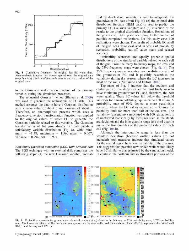
The sequential Gaussian method (Bleines et al. 2000)was used to generate the realizations of EC data. Thismethod assumes the data to have a Gaussian distributionwith a mean value of about 0 and variance of about 1.Therefore, an anamorphosis process which uses afrequency-inversion transformation function was appliedto the original values of water EC to generate theGaussian variable related to this variable. The Gaussiantransformation of Juá groundwater EC data yields asatisfactory variable distribution (Fig. 8), with: mini-mum = −1.58; maximum = 1.56; mean = 0.007;variance = 0.994; SD = 0.997.

Sequential Gaussian simulation (SGS) with external driftThe SGS technique with an external drift comprises thefollowing steps: (1) the new Gaussian variable, normal-

ized by de-clustered weights, is used to interpolate thegroundwater EC data (from Fig. 6); (2) the external driftdistribution function (HEM data) is used to predict theprimary EC Gaussian variable; and (3) inversion of theresults to the original distribution function. Repetitions ofthe process will take place according to the number ofpossible completed realizations. For this study case, 100realizations were chosen. The results of probable EC at allof the grid cells were evaluated in terms of probabilityscenarios, probability cut-off value maps and relatedaccuracy.

Probability scenarios are equally probable spatialdistributions of the simulated variable related to each cellof the grid. From the many frequency maps, the 25% andthe 75% frequency maps were chosen (Fig. 9a, b). The75% frequency map represents a more realistic scenario ofthe groundwater EC and it possibly resembles thevariability during dry season, where the EC increases inmost of the wells (Veríssimo and Feitosa 2002).

The maps of Fig. 9 indicate that the southern andcentral parts of the study area are the most likely areas tohave minimum groundwater EC, and, therefore, the bestwater quality. These EC values fall below the thresholdindicator for human potability, equivalent to 160 mS/m. Aprobability map of 90% depicts a more pessimisticscenario, where the EC values exceed up to 9 times thepotability limit for more than half of the Juá area. Thevariability (uncertainty) associated with 100 realizations ischaracterized statistically by measures such as the stand-ard deviation and the inter-quartile range (the third quartileminus the first quartile) of the predicted values for eachcell (Fig. 10a,b).

Although the inter-quartile range is less than thestandard deviation (because outlier values are notincluded) both measures indicate that simulated valuesfor the central region have least variability of the Juá area.This suggests that possible new drilled wells would likelyhave EC similar to that estimated by the simulation model.In contrast, the northern and southwestern portions of the

1000

500

0 -2 -1 0 1 2Gaussian Values

Ele

ctric

alC

ondu

ctiv

ity (

mS

/m)

Fig. 8 Cumulative frequency for original Juá EC water data.Anamorphosis function (dot curve) applied onto the original data(step function). Horizontal lines refer to min. and max. values of theoriginal data

Fig. 9 Probability scenarios for groundwater electrical conductivity (mS/m) in the Juá area: a 25% probability map; b 75% probabilitymap. Black squares refer to drilled wells and red squares are the new wells used for validation. Label RM1&c represents the drilled wellRM_1 and the dug well RM1_c

912

Hydrogeology Journal (2010) 18: 905–916 DOI 10.1007/s10040-010-0582-4

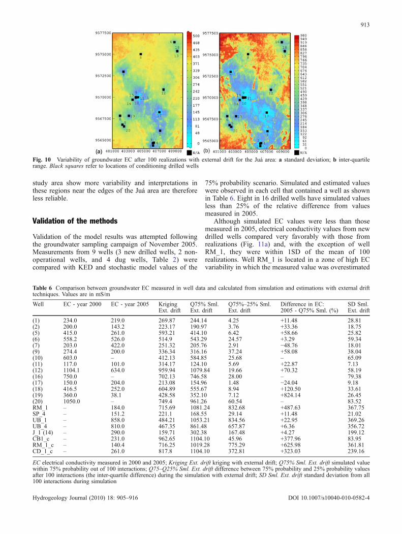
study area show more variability and interpretations inthese regions near the edges of the Juá area are thereforeless reliable.

Validation of the methods

Validation of the model results was attempted followingthe groundwater sampling campaign of November 2005.Measurements from 9 wells (3 new drilled wells, 2 non-operational wells, and 4 dug wells, Table 2) werecompared with KED and stochastic model values of the

75% probability scenario. Simulated and estimated valueswere observed in each cell that contained a well as shownin Table 6. Eight in 16 drilled wells have simulated valuesless than 25% of the relative difference from valuesmeasured in 2005.

Although simulated EC values were less than thosemeasured in 2005, electrical conductivity values from newdrilled wells compared very favorably with those fromrealizations (Fig. 11a) and, with the exception of wellRM_1, they were within 1SD of the mean of 100realizations. Well RM_1 is located in a zone of high ECvariability in which the measured value was overestimated

Fig. 10 Variability of groundwater EC after 100 realizations with external drift for the Juá area: a standard deviation; b inter-quartilerange. Black squares refer to locations of conditioning drilled wells

Table 6 Comparison between groundwater EC measured in well data and calculated from simulation and estimations with external drifttechniques. Values are in mS/m

Well EC - year 2000 EC - year 2005 KrigingExt. drift

Q75% Sml.Ext. drift

Q75%–25% Sml.Ext. drift

Difference in EC:2005 - Q75% Sml. (%)

SD Sml.Ext. drift

(1) 234.0 219.0 269.87 244.14 4.25 +11.48 28.81(2) 200.0 143.2 223.17 190.97 3.76 +33.36 18.75(5) 415.0 261.0 593.21 414.10 6.42 +58.66 25.82(6) 558.2 526.0 514.9 543.29 24.57 +3.29 59.34(7) 203.0 422.0 251.32 205.76 2.91 −48.76 18.01(9) 274.4 200.0 336.34 316.16 37.24 +58.08 38.04(10) 603.0 – 412.13 584.85 25.68 – 65.09(11) 117.0 101.0 314.17 124.10 5.69 +22.87 7.13(12) 1104.1 634.0 959.94 1079.84 19.66 +70.32 58.19(16) 750.0 – 702.13 746.58 28.00 – 79.38(17) 150.0 204.0 213.08 154.96 1.48 −24.04 9.18(18) 416.5 252.0 604.89 555.67 8.94 +120.50 33.61(19) 360.0 38.1 428.58 352.10 7.12 +824.14 26.45(20) 1050.0 – 749.4 961.26 60.54 – 83.52RM_1 – 184.0 715.69 1081.24 832.68 +487.63 367.75SP_4 – 151.2 221.1 168.55 29.14 +11.48 21.02UB_1 – 858.0 484.21 1053.21 834.56 +22.95 369.26UB_4 – 810.0 467.35 861.48 657.87 +6.36 356.72J_1 (14) – 290.0 159.71 302.38 167.48 +4.27 199.12CB1_c – 231.0 962.65 1104.10 45.96 +377.96 83.95RM_1_c – 140.4 716.25 1019.28 775.29 +625.98 361.81CD_1_c – 261.0 817.8 1104.10 372.81 +323.03 239.16

EC electrical conductivity measured in 2000 and 2005; Kriging Ext. drift kriging with external drift; Q75% Sml. Ext. drift simulated valuewithin 75% probability out of 100 interactions; Q75–Q25% Sml. Ext. drift difference between 75% probability and 25% probability valuesafter 100 interactions (the inter-quartile difference) during the simulation with external drift; SD Sml. Ext. drift standard deviation from all100 interactions during simulation

913

Hydrogeology Journal (2010) 18: 905–916 DOI 10.1007/s10040-010-0582-4

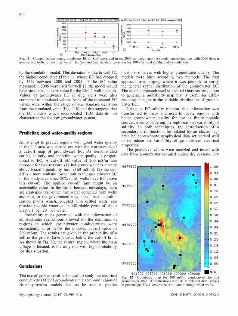
by the simulation model. This deviation is due to well 12,the highest conductive (Table 1), whose EC had droppedby 43% between 2000 and 2005. If the EC valuemeasured in 2005 were used for well 12, the model wouldhave simulated a closer value for the RM_1 well position.Values of groundwater EC in dug wells were alsocompared to simulated values. None of the measured ECvalues were within the range of one standard deviationfrom the simulated value (Fig. 11b) and this suggests thatthe EC models which incorporated HEM data do notcharacterize the shallow groundwater system.

Predicting good water-quality regions

An attempt to predict regions with good water qualityin the Juá area was carried out with the construction ofa cut-off map of groundwater EC. As demonstratedearlier, salinity, and therefore water quality, is propor-tional to EC. A cut-off EC value of 200 mS/m wasimposed for two reasons: (1) Juá groundwater is alreadyabove Brazil’s potability limit (160 mS/m); (2) the cut-off is a more realistic lower limit to the groundwater ECin the study area since 80% of all wells have EC abovethis cut-off. The applied cut-off limit might be anacceptable value for the locals because nowadays, thereare strategies that either mix water collected from wellsand rain, or the government may install small desalin-ization plants which, coupled with drilled wells, canprovide potable water at an affordable price of aboutUS$ 0.1 per 20 l of water.

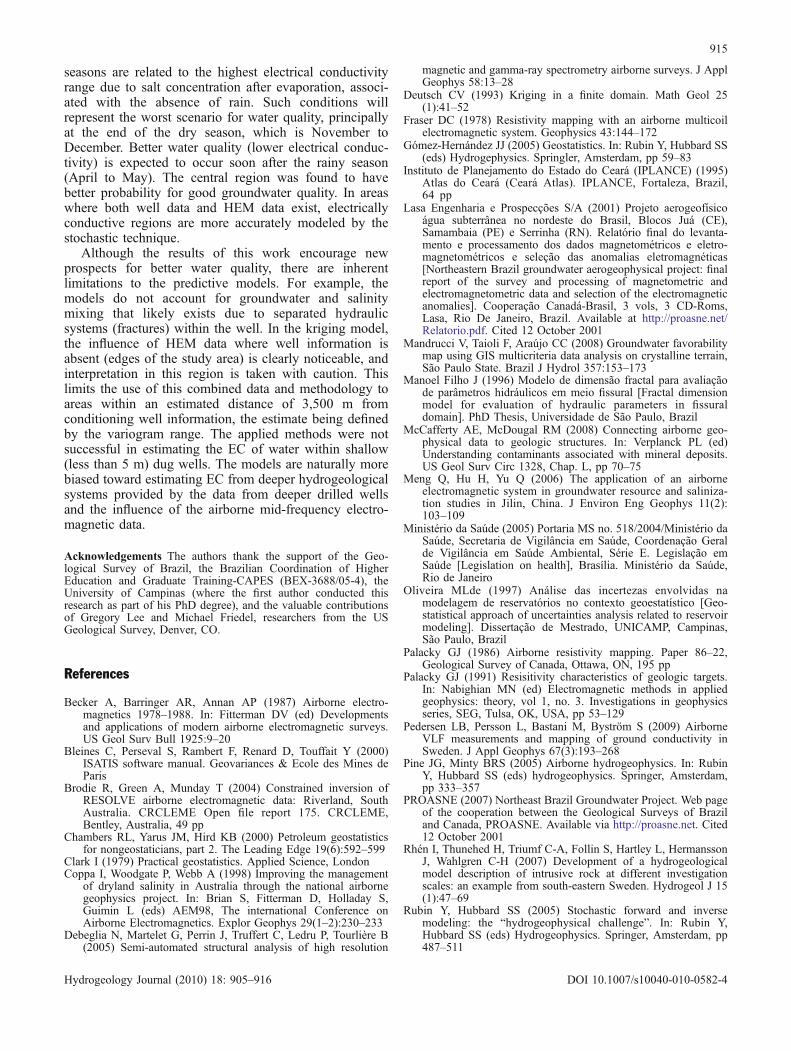
Probability maps generated with the information ofall stochastic realizations allowed for the definition ofregions in which groundwater conductivities wereconsistently at or below the imposed cut-off value of200 mS/m. The results are given in the probability of acell in the grid to have a value below the cut-off limit.As shown in Fig. 12, the central region, where the mainvillage is located, is the only one with high probabilityfor this situation.

Conclusions

The use of geostatistical techniques to study the electricalconductivity (EC) of groundwater in a semi-arid region ofBrazil provides models that can be used to predict

locations of areas with higher groundwater quality. Themodels were built according two methods. The firstapproach used kriging where it was possible to verifythe general spatial distribution of the groundwater EC.The second approach used sequential Gaussian simulationto generate a probability map that is useful for differ-entiating changes in the variable distribution of ground-water EC.

Using an EC-salinity relation, this information wastransformed to maps and used to locate regions withbetter groundwater quality for use as future potablesources, even considering the high seasonal variability ofsalinity. In both techniques, the introduction of asecondary drift function, formulated by an electromag-netic helicopter-borne geophysical data set, served wellto reproduce the variability of groundwater electricalproperties.

The predictive values were modeled and tested withdata from groundwater sampled during dry seasons. Dry

Fig. 11 Comparisons among groundwater EC (mS/m) measured in the 2005 campaign and the simulations/estimations with 2000 data: anew drilled wells; b new dug wells. The bars indicate standard deviation for 100 electrical conductivity simulations

Fig. 12 Probability map for 200 mS/m conductivity for Juágroundwater after 100 realizations with HEM external drift. Valuesin percentage, black squares refer to conditioning drilled wells

914

Hydrogeology Journal (2010) 18: 905–916 DOI 10.1007/s10040-010-0582-4

seasons are related to the highest electrical conductivityrange due to salt concentration after evaporation, associ-ated with the absence of rain. Such conditions willrepresent the worst scenario for water quality, principallyat the end of the dry season, which is November toDecember. Better water quality (lower electrical conduc-tivity) is expected to occur soon after the rainy season(April to May). The central region was found to havebetter probability for good groundwater quality. In areaswhere both well data and HEM data exist, electricallyconductive regions are more accurately modeled by thestochastic technique.

Although the results of this work encourage newprospects for better water quality, there are inherentlimitations to the predictive models. For example, themodels do not account for groundwater and salinitymixing that likely exists due to separated hydraulicsystems (fractures) within the well. In the kriging model,the influence of HEM data where well information isabsent (edges of the study area) is clearly noticeable, andinterpretation in this region is taken with caution. Thislimits the use of this combined data and methodology toareas within an estimated distance of 3,500 m fromconditioning well information, the estimate being definedby the variogram range. The applied methods were notsuccessful in estimating the EC of water within shallow(less than 5 m) dug wells. The models are naturally morebiased toward estimating EC from deeper hydrogeologicalsystems provided by the data from deeper drilled wellsand the influence of the airborne mid-frequency electro-magnetic data.

Acknowledgements The authors thank the support of the Geo-logical Survey of Brazil, the Brazilian Coordination of HigherEducation and Graduate Training-CAPES (BEX-3688/05-4), theUniversity of Campinas (where the first author conducted thisresearch as part of his PhD degree), and the valuable contributionsof Gregory Lee and Michael Friedel, researchers from the USGeological Survey, Denver, CO.

References

Becker A, Barringer AR, Annan AP (1987) Airborne electro-magnetics 1978–1988. In: Fitterman DV (ed) Developmentsand applications of modern airborne electromagnetic surveys.US Geol Surv Bull 1925:9–20

Bleines C, Perseval S, Rambert F, Renard D, Touffait Y (2000)ISATIS software manual. Geovariances & Ecole des Mines deParis

Brodie R, Green A, Munday T (2004) Constrained inversion ofRESOLVE airborne electromagnetic data: Riverland, SouthAustralia. CRCLEME Open file report 175. CRCLEME,Bentley, Australia, 49 pp

Chambers RL, Yarus JM, Hird KB (2000) Petroleum geostatisticsfor nongeostaticians, part 2. The Leading Edge 19(6):592–599

Clark I (1979) Practical geostatistics. Applied Science, LondonCoppa I, Woodgate P, Webb A (1998) Improving the management

of dryland salinity in Australia through the national airbornegeophysics project. In: Brian S, Fitterman D, Holladay S,Guimin L (eds) AEM98, The international Conference onAirborne Electromagnetics. Explor Geophys 29(1–2):230–233

Debeglia N, Martelet G, Perrin J, Truffert C, Ledru P, Tourlière B(2005) Semi-automated structural analysis of high resolution

magnetic and gamma-ray spectrometry airborne surveys. J ApplGeophys 58:13–28

Deutsch CV (1993) Kriging in a finite domain. Math Geol 25(1):41–52

Fraser DC (1978) Resistivity mapping with an airborne multicoilelectromagnetic system. Geophysics 43:144–172

Gómez-Hernández JJ (2005) Geostatistics. In: Rubin Y, Hubbard SS(eds) Hydrogephysics. Springler, Amsterdam, pp 59–83

Instituto de Planejamento do Estado do Ceará (IPLANCE) (1995)Atlas do Ceará (Ceará Atlas). IPLANCE, Fortaleza, Brazil,64 pp

Lasa Engenharia e Prospecções S/A (2001) Projeto aerogeofísicoágua subterrânea no nordeste do Brasil, Blocos Juá (CE),Samambaia (PE) e Serrinha (RN). Relatório final do levanta-mento e processamento dos dados magnetométricos e eletro-magnetométricos e seleção das anomalias eletromagnéticas[Northeastern Brazil groundwater aerogeophysical project: finalreport of the survey and processing of magnetometric andelectromagnetometric data and selection of the electromagneticanomalies]. Cooperação Canadá-Brasil, 3 vols, 3 CD-Roms,Lasa, Rio De Janeiro, Brazil. Available at http://proasne.net/Relatorio.pdf. Cited 12 October 2001

Mandrucci V, Taioli F, Araújo CC (2008) Groundwater favorabilitymap using GIS multicriteria data analysis on crystalline terrain,São Paulo State. Brazil J Hydrol 357:153–173

Manoel Filho J (1996) Modelo de dimensão fractal para avaliaçãode parâmetros hidráulicos em meio fissural [Fractal dimensionmodel for evaluation of hydraulic parameters in fissuraldomain]. PhD Thesis, Universidade de São Paulo, Brazil

McCafferty AE, McDougal RM (2008) Connecting airborne geo-physical data to geologic structures. In: Verplanck PL (ed)Understanding contaminants associated with mineral deposits.US Geol Surv Circ 1328, Chap. L, pp 70–75

Meng Q, Hu H, Yu Q (2006) The application of an airborneelectromagnetic system in groundwater resource and saliniza-tion studies in Jilin, China. J Environ Eng Geophys 11(2):103–109

Ministério da Saúde (2005) Portaria MS no. 518/2004/Ministério daSaúde, Secretaria de Vigilância em Saúde, Coordenação Geralde Vigilância em Saúde Ambiental, Série E. Legislação emSaúde [Legislation on health], Brasília. Ministério da Saúde,Rio de Janeiro

Oliveira MLde (1997) Análise das incertezas envolvidas namodelagem de reservatórios no contexto geoestatístico [Geo-statistical approach of uncertainties analysis related to reservoirmodeling]. Dissertação de Mestrado, UNICAMP, Campinas,São Paulo, Brazil

Palacky GJ (1986) Airborne resistivity mapping. Paper 86–22,Geological Survey of Canada, Ottawa, ON, 195 pp

Palacky GJ (1991) Resisitivity characteristics of geologic targets.In: Nabighian MN (ed) Electromagnetic methods in appliedgeophysics: theory, vol 1, no. 3. Investigations in geophysicsseries, SEG, Tulsa, OK, USA, pp 53–129

Pedersen LB, Persson L, Bastani M, Byström S (2009) AirborneVLF measurements and mapping of ground conductivity inSweden. J Appl Geophys 67(3):193–268

Pine JG, Minty BRS (2005) Airborne hydrogeophysics. In: RubinY, Hubbard SS (eds) hydrogeophysics. Springer, Amsterdam,pp 333–357

PROASNE (2007) Northeast Brazil Groundwater Project. Web pageof the cooperation between the Geological Surveys of Braziland Canada, PROASNE. Available via http://proasne.net. Cited12 October 2001

Rhén I, Thunehed H, Triumf C-A, Follin S, Hartley L, HermanssonJ, Wahlgren C-H (2007) Development of a hydrogeologicalmodel description of intrusive rock at different investigationscales: an example from south-eastern Sweden. Hydrogeol J 15(1):47–69

Rubin Y, Hubbard SS (2005) Stochastic forward and inversemodeling: the “hydrogeophysical challenge”. In: Rubin Y,Hubbard SS (eds) Hydrogeophysics. Springer, Amsterdam, pp487–511

915

Hydrogeology Journal (2010) 18: 905–916 DOI 10.1007/s10040-010-0582-4

Santos AC (2000) Noções de hidroquímica [Notions on hydro-chemistry]. In: Feitosa FAC, Manoel Filho J (eds) Hidrogeologia:conceitos e aplicações, 2nd edn. CPRM/REFO, LABHID-UFPE,Fortaleza, Brazil

Sattel D, Kgotlhand L (2003) Modelling aquifer structures withairborne EM in the Boteti area, Botswana. Proceedings ofSymposium on the Application of Geophysics to Engineeringand Environmental Problems, April 2003, San Antonio, TX,USA

Silva OAda (2005) Análise de dados aerogeofísicos aplicada àexploração e ao gerenciamento de recursos hídricos subterrâ-neos [Analysis of airborne geophysical data applied to theexploration and management of groundwater resources]. PhDThesis, Institute of Geosciences, Universidade Federal da Bahia,Brazil, 88 pp. Available at http://www.pggeofisica.ufba.br/resumos/pdf/d042a.pdf. Cited 12 May 2008

Silva CMSV, Vasconcelos MB, Santiago MMF (2001) Recarga edatação de poços no cristalino [Recharge and dating of drilledwells in the crystalline domain]. In: IV Simpósio de Hidrogeo-logia do Nordeste, 2001, Recife. Anais do IV Simpósio deHidrogeologia do Nordeste, ABAS, São Paulo, Brazil, pp 8–14

Sousa MF, Albuquerque GA, Carvalho RR (1984) Cristalino naParaíba: resultado obtido pela CDRM-PB no âmbito doPrograma de Aproveitamento de Recursos Hídricos noNordeste – PROHIDRO/SUDENE [Crystalline in Paraíba:results of CDRM-PB during the Northeastern Program for theUse of Hydric Resources – PROHIDRO/SUDENE]. In:Congresso Brasileiro de Águas Subterrâneas. III, 1984.Fortaleza, Anais 1, pp 128–146

Souza Filho OAde (1998) Geologia e mapa de previsão deocorrência de água subterrânea. Folha SA.24-Y-D-V Irauçuba,Ceará [Geology and predictive map of groundwater occurrence,SA.24-Y-D-V Irauçuba sheet]. Dissertação de Mestrado. Uni-versidade Federal de Ouro Preto, Brasil, 99 pp

Souza Filho OAde, Ribeiro JÁ, Veríssimo LS, Oliveira RGde,Gomes FEM, Brandão RdeL, Frizzo SJ, Oliveira JFde (2003)Projeto otimização de metodologias para prospecção de águassubterrâneas em rochas cristalinas. Relatório integrado deatividades 1999–2002: Bases para avaliação do projeto [Projectfor optimization of groundwater prospection methodologies incrystalline rocks: integrated report 1999–2002]. CPRM/REFO.Fortaleza, Brazil, 160 pp

Souza Filho OAde, Veríssimo LS, Silva CMS, Santiago MMF,Santiago MF (2004) Medidas hidroquímicas nas águas sub-

terrâneas da região de Irauçuba, Norte do Ceará [Hydrochemicalmeasures in Irauçuba groundwaters, north of Ceará]. In:Congresso Brasileiro de Águas Subterrâneas XIII, 2004.Cuiabá, CD-Rom. Available at http://www.cprm.gov.br/publique/media/medidas_hidroq.pdf. Cited 1 May 2007

Souza Filho OAde, Oliveira RG, Ribeiro JA, Veríssimo LS, Sá JU(2006) Interpretação e modelagens de dados de eletrorresistivi-dade para locações de poços tubulares no aqüífero fissural daárea-piloto Juá, Irauçuba-Ceará [Interpretation and modeling ofelectrical resistivity data for water well location in the fissuralaquifer of Juá study-area]. Rev Geol DEGEO/UFC 19(1):7–21.Available at www.revistadegeologia.ufc.br/01_2006.pdf. Cited3 April 2007

Souza Filho OAde, Silva AM, McCaffertty AE, Perrotta MM,Deszczpan M, fitterman D (2007a) Geophysical propertiesassociated to Juá district geology, Ceará, Brazil. In: 10thInternational Congress of the Brazilian Geophysical Society,SBGf, Rio de Janeiro, April 2007, CD-Rom

Souza Filho OAde, McCaffertty AE, Silva AM, Perrotta MM(2007b) Ground-water potential: a predictive model fromairborne geophysical, radiometric, and remote sensing data,Ceará, Brazil. In: Simpósio Brasileiro de SensoriamentoRemoto (SBSR), 13, April 2007, Florianópolis, Brazil, pp3593–3595, CD-ROM. Available at http://marte.dpi.inpe.br/col/dpi.inpe.br/sbsr@80/2006/11.15.17.35.52/doc/3593-3595.pdf.Cited 15 May 2007

Speed R (2002) Airborne geophysics for catchment management:why and where. Explor Geophys 33:51–56

Telford WM, Geldart LP, Sheriff RE, Keys DA (1984) Appliedgeophysics. Cambridge University Press, New York, pp442–457

Veríssimo LS, Feitosa FAC (2002) As águas subterrâneas noNordeste do Brasil. Região de Irauçuba - Estado do Ceará,Brasil [Groundwater in Northeast Brazil. Irauçuba Region–Stteof Ceará]. In: Congresso da Associação Internacional deHidrogeologia, XXXII e Congresso da Associação Latino-Americana de Hidrologia Subterrânea, VI, 2002, Mar Del Plata,Argentina, pp 889–896, CD-Rom. Available at http://proasne.net/CongALHSUD_Liano.pdf. Cited 10 January 2010

Wackernagel H (1995) External drift. In: Multivariate geostatistics:an introduction with applications. Springer, Berlin, pp 190–200

Wynn F (2002) Evaluating groundwater in arid lands using airbornemagnetic/EM methods: an example in the southwestern U.S.and northern Mexico. The Leading Edge 1(21):62–64

916

Hydrogeology Journal (2010) 18: 905–916 DOI 10.1007/s10040-010-0582-4