Using Sequence Analysis to Understand CareerProgression: an Application to the UK House of

Commons∗

Matia Vannoni† & Peter John‡

August 14, 2018

Abstract

We argue that sequence analysis, mainly used in sociology, may be effectively deployedto investigate political careers inside legislatures. Career progression is a classic topicin political science, but political scientists have mainly examined access to legislatures.Although data reduction methods, for instance, can provide insight, we argue thatsequence analysis can be used to understand better the career patterns inside parlia-ments. In this paper, we explain the method. Then we show how it can describesteps in political careers and map different patterns of advancement. We apply se-quence analysis to a case study of MPs in the UK House of Commons from 1997 to2015. We describe the variety of career paths and carry out regression analysis on thedeterminants of MP career progression.

Keywords: Sequence analysis, legislative careers, elite studies

∗We thank colleagues in the UCL Grand Challenges project Mapping Policy with Big Data: the HealthPolicy Agenda and its Networks for sharing data. We greatly appreciate the comments of Hugh Ward onan early draft of the paper. We are also grateful to colleagues at UCL who came to hear the paper at theDepartment of Political Science seminar on 15 October 2014 and who made many constructive suggestions.We also thank Moritz Osnabruegge for helpful comments on the latest draft. Replication files for this paperare located at https://doi.org/10.7910/DVN/I8YHPT.

†IGIER, Bocconi University, Via Rontgen 1, 20136 Milano, Italy; email: matia.vannoni@unibocconi.it‡Department of Political Economy, King’s College London, Bush House Aldwych, London WC2B 4PH

1

Introduction

With a few exceptions (Guttsman 1963; Kam et al. 2010; Allen 2012), studies of career

progression have focused on access to legislatures. This dependent variable suits regression

or duration analysis as what is explained is entry into the elite as a function of ascribed

characteristics, such as education and gender. Political scientists, however, have tended

to neglect what happens later on during legislators’ careers, in particular the various routes

legislators take when seeking office once elected, which can offer greater understanding about

how political careers reflect different choices and opportunities. Although methods, such as

cluster analysis, offer insight into career paths, we suggest that sequence analysis is better

able to show how the composition of the elite is a function of the career path that has been

followed. Sequence analysis seeks to account for different combinations of paths and offers an

alternative set of metrics to analyse the determinants of career progression. So far, sequence

analysis has not been utilized very much in political science, nor has it been applied to career

progression within legislatures. We seek to remedy this relative neglect of the method and

show its advantages for understanding political careers.

In this paper, we first introduce the key methods of elite studies as applied to political

careers. Then we set out sequence analysis as a method and explain its elements. In the

discussion, which is more fully elaborated in the appendix, we compare sequence analysis

to other methods of examining patterns in elite progress, such as cluster analysis. To show

the scope and range of the method, we apply sequence analysis to a case study of career

progression in the UK House of Commons for the period 1997-2015.

Elite Study Methods

Elite studies have so far treated stages of career at different points in time as independent,

usually as separate variables. Becoming Prime Minister, for example, is assumed not to be

a function of previously being Chancellor of the Exchequer, or a Minister of State. But

2

it is likely the Prime Minister has been, say the Home Secretary, in a prior office, or in a

senior post on the opposition benches. It likely that there are patterns to career progression,

reflecting well-known paths and steps, and a degree of differentiation between the type of

politician as to how these steps are taken.

An alternative method of understanding progression in political careers is survival anal-

ysis (or event history analysis), which has already been used in elite studies (Curtin, Kerby,

and Dowding 2015). The latter predicts the probability of a future state to occur given the

presence of past states. Nonetheless, this method focuses more on the transition from a

state to another rather than measuring the career paths in their entirety. It focuses on the

likelihood that the individual will undergo a transition to a determined career stage taking

into consideration previous career steps and their order. This method does not describe

or compare career paths.1 Finally, time series analysis might be appropriate, but is not

valid in this context as it best used with continuous variables with a large number of time

points while career data are categorical and usually measured at a very few points in time

(Blanchard 2011). Furthermore, the requirement that time points need to be equally distant

from one another on a temporal scale (unnecessarily) restricts the applications of career path

analysis. Like survival analysis, time series analysis is not tailored to measure career paths.

Data reduction can overcome this, by providing a single measure to account for the

similarities and differences between career paths, which takes into consideration their entirety

and not a single ‘jump’, like survival analysis. The main idea is that the stages of the career

of an individual, what can be labeled career data, should not be treated as independent,

but each stage should relate to each other. Massoni, Olteanu, and Rousset (2009) identify

two data reduction methods to study careers: factor analysis and cluster analysis. Although

they are an improvement on the current methods in elite studies and political economy, there

are drawbacks. When used alone, the methods do not take into consideration two crucial

aspects in career progression: the duration of careers and the order of career stages. In

1. The same holds true for more recent duration models, such as Markov-transition models, which areused to study conditions that have events that occur repeatedly over time.

3

the Appendix, using the same data, we compare cluster analysis with the method proposed

below, showing that only the latter can account for these two important aspects of careers.

Sequence Analysis: the Method Explained

Brzinsky-Fay, Kohler, and Luniak (2006) explain that ‘a sequence is defined as an ordered list

of elements, where an element can be a certain status’ (p. 436). Sequence data takes the form

of categorical time series data, where elements may refer to relative and not absolute points in

time (Brzinsky-Fay, Kohler, and Luniak 2006). In contrast to longitudinal data, time points

in sequence analysis must meet only one criterion, namely being ordered across the sample,

but they do not necessarily need to be equally distant from one another on a temporal scale.

Assume that the career of an MP in the House of Commons is measured in six years using

the following elements, explained in details below: backbenchers, frontbenchers, and Great

Offices of State, the most prestigious positions in the cabinet. Examples of sequences that

can be found in the sample are:

1. BB − BB − BB − FB − FB − GO

2. BB − BB − BB − GO − GO − GO

3. BB − BB − FB − FB − FB − GO

4. BB − BB − BB − FB − BB − GO

The first two MPs have different career paths: the former has gone from the back-bench

through the front-bench to the Great Offices of State while the latter has by-passed the

front-bench stage moving directly from the back-bench to the most prestigious positions.

The elements that compose the sequences are the first things to look at when analyzing

sequences. Nonetheless, two other aspects matter: the order of elements and the duration

of episodes. Indeed, the first, the third and the fourth sequences share the same elements.

4

Yet the first sequence is more similar to the third one than to the fourth one in that they

share the same order of elements and they differ only in the duration of episodes. The

latter are defined as sections of a sequence that consist of the same elements and in this

case they refer to BB − BB − BB and FB − FB in the first sequence and BB − BB and

FB − FB − FB in the third one. Sequence analysis takes into consideration the elements

which compose a sequence, their order, and the duration of episodes (Blanchard 2011). In

doing so, sequence analysis provides descriptive statistics and graphical visualizations as well

as a measure of distance between sequences, namely optimal matching, which can be used

to make inferences.

Optimal matching (OM) compares sequences on the basis of a complex algorithm, which

has already been used in several fields, especially biology.2 This measure compares sequences

by considering substitution costs (Needleman and Wunsch 1970). The algorithm compares

sequences by pairs and it associates to each pair a distance index based on the cost of

replacement of different elements. In this vein, substitutions take into consideration the

differences in elements between sequences.

Optimal matching considers also indel costs, namely the costs of insertions and deletions

of elements, to account not only for the differences between elements but also for their order

and the duration of episodes (Blanchard 2011; Brzinsky-Fay, Kohler, and Luniak 2006).

As seen above, the first sequence differs from the third and the fourth ones for only one

element. In this vein, if we consider only substitutions the distance indexes between them

will be the same. Nonetheless, as noticed above, the first sequence differs from the third

only in the duration of episodes. Accordingly, it suffices to insert a gap before the GO in the

first sequence and to insert a gap before the first FB in the third to make those sequences

identical:

BB − BB − BB − FB − FB − XX − GO

BB − BB − XX − FB − FB − FB − GO

2. We acknowledge the existence of other algorithms, such as the Longest Common Prefix and the LongestCommon Subsequence (Studer et al. 2011). Yet, optimal matching is the common practice in social research.

5

It should be noted how the same outcome can be obtained by deleting certain elements

from the sequences. Optimal matching takes into consideration also this aspect by differen-

tiating between substitutions and indels.3

Sequence analysis is common in sociology (Halpin and Cban 1998; Abbott and Hrycak

1990; Blair–Loy 1999; Stovel, Savage, and Bearman 1996). For instance, it has been used to

study the careers of French economic elites (Lemercier 2005) and social movement activists

(Blanchard 2005; Fillieule and Blanchard 2011). It has recently started to appear in political

science and, more specifically, in elite studies, as reviewed by Blanchard, Bühlmann, and

Gauthier (2014) and Blanchard (2011). Some recent applications include the study of the

careers of: Spanish junior ministers in Teruel and Real-Dato (2014), German state secretaries

in Tepe and Marcinkiewicz (2013), German MPs’ in Ohmura et al. (2018), German Federal

Constitution Court judges in Jäckle (2016) and in-house lobbyists in companies in Coen and

Vannoni (2016). Yet, no application of this method can be found in the analysis of elected

politicians inside the parliament, one of the classic topics in elite studies.

Empirical Application of the Method: Careers in the

UK House of Commons

This section of the paper applies sequence analysis to the study of careers in the House of

Commons. In this case study, we show how the method can allow researchers to test the

findings in (British) elite studies and more recent political economy approaches to identify

what might be the main determinants of careers in the House of Commons. First, we focus

on the social and economic background of politicians. Early writers were keen to map the

background of the elite (Domhoff 1967; Miliband 1969; Mills 1956; Guttsman 1963; King

1981; Mellors 1978; Putnam 1976; Czudnowski 1970, 1972). The idea draws from classic

elite theory which is concerned about the concentration of people from elite backgrounds

3. A detailed explanation on how optimal matching works is provided in the Appendix.

6

into positions of power or the circulation of elites, claims that appear in the foundational

studies of political science (Hunter 1953; Schattschneider 1975; Michels, Paul, and Paul

1915). The main focus remained on the representativeness of the British political elites—

in terms of ascriptive features, such as wealth—across the political hierarchy, namely from

voters through activists, local leaders, backbenchers and frontbenchers in Parliament, and

across to political parties.

In the 1970s and 1980s attention shifted from the representativeness of political elites

in terms of socio-economic factors to ethnic background and sex/gender (Kirkpatrick 1974;

Norris and Lovenduski 1995; Studlar and McAllister 1991; Andersen and Thorson 1984;

Rosaldo, Lamphere, and Bamberger 1974; Lawless and Theriault 2005). At the same time,

writers moved from exploratory analyses to explanations of career progression, concentrating

also on exogenous factors, such as party recruitment and the type of election (Eliassen and

Pedersen 1978; Seligman 1961; Thurber 1976). In the 1990s and 2000s, career progression

attracted the attention of students of political economy. Based on the public choice literature

(Stigler 1972; Wittman 1989), which advocated that political competition both inside and

outside parties leads to optimal political outcomes, this line of research focused on the quality

of political candidates (Diermeier, Keane, and Merlo 2005; Mattozzi and Merlo 2008; Merlo,

Landi, and Mattozzi 2009) as well party selection (Galasso and Nannicini 2011), a concern

that also appears in comparative elite studies (Best and Cotta 2000; Best et al. 2001; Best

and Edinger 2005; Best and Higley 2014; Best, Lengyel, and Verzichelli 2012; Almeida, Pinto,

and Bermeo 2003; Ilonszki 1998; Müller-Rommel, Fettelschoss, and Harfst 2004; Semenova,

Edinger, and Best 2013; S, tefan-Scalat 2004) and in work on British politics (Denver and

Garnett 2014; Fisher and Wlezien 2013; Kavanagh and Cowley 2010; Bennie, Rallings, and

Tonge. 2002; Butler and Kavanagh 1980, 1992; McCallum and Readman 1947; Cook and

Stevenson 2014).4

4. In the US the attention has also been on careers outside legislatures (Maddox 2004).

7

Data and Measurement

Career progression of British MPs in the House of Commons is analysed with a dedicated

dataset that contains data on the demographic characteristics as well as on the educational

and professional background of all MPs active in four legislatures of the British House of

Commons: 1997-2001, 2001-2005, 2005-2010 and 2010-2015, who entered the House in or

after 1997. The data contain membership of the cabinets at secretary level and also on the

shadow cabinets—that is the leadership groups of the opposition parties and differentiate

ranks within the (shadow) cabinet.

The dataset has a good level of variation in terms of MPs’ individual characteristics, the

composition of the House of Commons as well as of the (shadow) cabinets. Firstly, it contains

all the MPs who have been active in the last four legislatures and who entered the House in or

after 1997. Accordingly, data spans over almost 20 years, which is arguably a sufficient time

for a generational change to occur in the Parliament thus controlling for a potential cohort

effect. Secondly, since 1997 the UK has had two consecutive cabinets led by the Labour

party and a coalition cabinet led by the Conservative Party in cooperation with the Liberal

Democrats. Thirdly, official cabinets and shadow cabinets have undergone several reshuffles

every year during that period: in 2010-2013 the coalition government cabinet underwent ten

reshuffles and the Labour shadow cabinet five, roughly a third of which entailed the inclusion

of new MPs.

The career paths of MPs inside the House are measured for each year from 1997 to

2014. Three elements are measured: backbench (BB), frontbench (FB) and Great Offices

of State (GO). The latter comprises the Prime Minister, the Deputy Prime Minister, the

Chancellor of the Exchequer, the Foreign Secretary and the Home Secretary as well as the

respective roles in the shadow cabinets of the opposition parties. Frontbench measures all

the individuals sitting in the (shadow) cabinet at secretary level and the respective leaders

of the House.5 It should be noted that data are gathered not only for the official opposition

5. Although the Liberal Democrats formed a shadow cabinet after the 1997 general elections, it remained

8

but also for the party with the third largest share of seats in the House. For instance, in

the period 1997-2010 the shadow cabinet of the Liberal Democrat party is considered. This

allows to better account for representativeness along the political hierarchy. Although we

acknowledge that more fine-grained measures of cabinet offices are present in the literature

(Allen 2012), using few categories makes the interpretation of results with the method used

here easier. Indeed, rarely do studies using sequence analysis employ more than three or four

categories. Moreover, these categories are externally valid, as a similar hierarchy of positions

are found in most parliamentary systems.

The educational and professional background of MPs is also included in the dataset.

More specifically, we have data on secondary school, university and previous occupation.

The first one is measured with a dummy variable with value 1 for state school and 0 for

private school (fee paying). The university variable associates value 0 to the non-attendance

of university, value 1 for undergraduate education and value 2 for postgraduate education.

Finally, previous profession is measured with a dummy variable on whether they had had a

‘instrumental’ occupation before entering the House. Instrumental jobs are those occupations

which according to a well established tradition in elite studies are supposed to make the jump

to the political career easier (Allen 2012).6

Other variables dealing with individual factors are included in the analysis: gender and

age at entry in Parliament. Other actors are also considered: party affiliation and whether

the MP was elected in a general election or in a by-election.7 Lastly, we control for the

legislature of entry.8 Data was drawn from several sources: Dod’s Parliamentary Companion

very fluid until 1999 and it was characterised by many reshuffles until 2007. It is crucial to control for theparty in the analysis below.

6. For a complete list see Figure 1 in Allen (2012).7. In this analysis we consider only those MPs which belong to the three main parties in the House. The

reason is that only these MPs have a chance to enter the (shadow) cabinet.8. The categorical variable Legislature is operationalized in order of time, namely value 1 stands for the

1997-2001 legislature and so on and so forth. We do not cluster standard errors on the legislature of entryand instead we use robust standard errors. The reason is that cluster robust standard errors are likelyto produce (downward) biased results where the number of clusters is small (Esarey and Menger 2018).Although dependency between observations in clusters might be present in our analysis (hence leading tounderestimated standard errors too), the benefits of using robust standard errors arguably outweigh thoseof clustered standard errors in this analysis.

9

Guide to the General Election, Who’s Who, BBC News, TheyWorkForYou, The Guardian,

Politics.co.uk, Gov.uk and MPs’ personal websites.9 Table A1-A3 in the Appendix show the

descriptive statistics.10

Results

We calculate distances between pairs of sequences in order to cluster those distances and

derive ideal-typical sequences (or career paths). We do so with the help of the R package

TraMiner (Studer et al. 2011). More information on this package can be found in the

Appendix. As this represents the first study of career progression inside the parliament

with this method, we are agnostic with respect to the number of career paths we find and

their characteristics. In this vein, the approach is entirely data driven. We choose eight

career types, which explain 81 per cent of the variation across sequences in the sample. The

R package TraMiner has a function which tells the researcher what number of groups has

the highest R squared. The other clustering options and the relative R squared values are

presented in the Appendix, respectively in Figure A1-A4 and in Table A4. The Appendix

also provides an explanation of the clustering functions in the TraMiner package.

Figure 1 shows the eight ideal-typical career paths. The vertical axes of the quadrants

in Figure 1 show the frequencies of the states in every cluster (close in spirit to a traditional

stacked bar chart). On the horizontal axis we display time. It should be noted that, as it

is common practice in sequence analysis, missing values are not treated like separate states

but are deleted.11 Those MPs who stay in the House for a shorter period than that under

analysis have shorter sequences. In this particular case, the clustering process groups shorter

sequences together, regardless of whether the MP enters the House later or leaves earlier.

The reason is that in this particular case shorter sequences tend to be similar with respect

to the elements which compose them and their order. As a result, values on the horizontal

9. Data gathering occurred in spring and summer 2014.10. Future research should also includes less tangible factors, such as MPs’ ideology, as done in Kam et

al. (2010).11. An explanation of how missing data are treated can be found in the Appendix.

10

axes in Figure 1 do not have a substantive meaning: value 1 in the top-left quadrant and in

the top-right quadrant do not necessarily refer to the same year.

[Figure 1 here]

The majority of MPs remain in the backbench throughout their careers, but some stay

longer in the House (Career 8 in Figure 1) whereas others stay for shorter periods of time

(Career 1 and Career 2 in Figure 1). Then, a large number of MPs enter as backbenchers

and after some time they make their way to the Great Offices of State, but then leave the

house earlier than others (Career 5 in Figure 1). Some MPs gradually reach the frontbench

and then eventually occupy the Great Offices of State (Career 4 in Figure 1), while others

move to immediately to the frontbench, but then they go back to the backbenches (Career

3 in Figure 1). Then there are MPs who enter the House as frontbenchers and remain so

throughout their careers. While some reach the Great Offices of State (Career 7 in Figure

1), others do not (Career 6 in Figure 1). As can be seen in the Appendix, the results from

other clustering options, especially those with six and seven groups, are not very different

from those presented here.

We now investigate the determinants of MP career progression in the House of Commons.

Table 1 shows the results of the multinomial regression analysis with the eight clusters derived

above as categories of the dependent variable. For simplicity, we take Career 1 as baseline

category. This is a reasonable choice, as we are interested in what affects the different MP

career paths with respect to the most frequent path, namely the one composed only by

backbencher values. The sample contains MPs active in different legislatures which might

influence career progression. It is likely that MPs entering the House in a specific legislative

session have something in common, which in turn makes their career progression similar with

respect to other MPs. We control also for the session of entry.12 Table A5 and Table A6 in

12. Our sample is not perfectly balanced and only captures a picture of career progression. Some MPsenter the sample at later stages, because elected in by-elections or simply in one of the general electionsheld after 1997; and others leave at earlier stages, because they lose elections. Our approach takes this intoconsideration, by clustering together shorter sequences.

11

the Appendix show the results with the clustering at six and seven groups, respectively.

First, we find that the gender of the MP does not strongly affect career progression

in the House. Indeed, the coefficient of gender is not statistically significant across the

different specifications. We find that gender does not affect the political career, once the

individual enters the parliament. It might be that the gender bias is strong at the entrance to

parliament, but once inside, women enjoy the same career opportunities than men. Second,

findings on the social background of MPs show that although access to the high ranks is not

completely precluded for those from state schools, they tend to be less associated with those

career types with high frequency of Great Offices of State (Career 5 and Career 7 in Figure

1). Individuals from modest backgrounds can make it to the top of the political ladder, even

if inequality is present.13 This finding is in line with the picture of British politics depicted

by the media, with people from different backgrounds getting to the top, but with some

inequality still present.

Third, having a university degree is not prerequisite for entering the cabinet. Again, this

might be because higher education is necessary to enter the parliament but once inside it,

other factors matter more. Fourth, the age at which the MP enters the House is negatively

related to Career 4 and Career 8, which means that those MPs who enter the House when

they are older tend not to have long and gradual careers. Fifth, the professional experience

of MPs does not seem to affect their career in the House. Finally, the party and the type

of election determine MPs’ career progression. Conservative MPs are more likely to make it

to the top, but then to go back to the backbench, compared to Labour MPs. However, the

results for party might be driven by several factors, such as the number of seats allocated to

different parties, the times that party was in power and the structure of its shadow cabinets.

We find that a MP elected in a by-election is more likely to make it to the cabinet, which

13. In the Appendix, we take the sub-sample of MPs with a university degree and we check whether havingattended Oxford or Cambridge affects the MP’s career (Table A7). We find that Oxbridge MPs (whichrepresents roughly the 28 per cent of all the MPs) are less likely to have a career of the type Career 6 andCareer 8, where backbench positions are more frequent. This suggests that a sort of elitism is still in placein British politics, also inside the House of Commons.

12

provides evidence that parties use by-elections as a way to place prominent candidates in

office .

To validate our results, we also run what the methodology literature on sequence analysis

calls discrepancy analysis. This type of analysis measures the share of the variation of

the sequences explained by a variable and also the significance of the association. More

specifically, close in spirit with a multivariate ANOVA, it provides for each covariate the

effect measured when removing the covariate from the full model with all variables included.

More details are provided in the Appendix. Results support the findings, suggesting a

strong effect of the age at entry as well as party and legislative session (see Table A8 in the

Appendix).

[Table 1 here]

Conclusion

Sequence analysis provides additional insights in the analysis of political careers. It is a

valid and reliable way to measure career paths, which can be used to describe and compare

them, as well as to identify recurrent ones. Sequence analysis also provides a way to measure

the distance between careers and thus to derive valid proxies that can be used in regression

analysis. To encourage its wider adoption in the study of political careers, we have explained

the method and then applied it to a case study of UK MPs.

In this case study, we find that expected relationships between ascriptive characteristics

and career progression were not found. Researchers using sequence analysis could probe the

interaction between stages of the political hierarchy, such as entry to the parliament and

career progression therein. Selection within disadvantaged groups—in terms of gender and

ethnic background, for instance—may be so tough in the earlier stages that those legislators

who get through have acquired the necessary skills to rise in the hierarchy. We believe

that political scientists who are interested in careers will use sequence analysis as a useful

13

complement to existing methods.

14

References

Abbott, A., and A. Hrycak. 1990. “Measuring Resemblance in Sequence Data: An Optimal

Matching Analysis of Musicians’ Careers.” American Journal of Sociology 96 (1): 144–

185.

Allen, P. 2012. “Linking Pre-parliamentary Political Experience and the Career Trajectories

of the 1997 General Election Cohort.” Parliamentary Affairs 66 (4): 685–707.

Almeida, P. T. d., A. C. Pinto, and N. G. Bermeo. 2003. Who Governs Southern Europe?:

Regime Change and Ministerial Recruitment, 1850-2000. London: F. Cass.

Andersen, K., and S. J. Thorson. 1984. “Congressional Turnover and the Election of Women.”

Political Research Quarterly 37 (1): 143–156.

Bennie, L., C. Rallings, and J. Tonge. 2002. The 2001 General Election. London: Taylor &

Francis Group.

Best, H., V. Cromwell, C. Hausmann, and M. Rush. 2001. “The Transformation of Legislative

Elites: The Cases of Britain and Germany since the 1860s.” The Journal of Legislative

Studies 7 (3): 65–91.

Best, H., and J. Higley. 2014. Political Elites in the Transatlantic Crisis. Basingstoke: Pal-

grave Macmillan.

Best, H., and M. Cotta. 2000. Parliamentary Representatives in Europe, 1848-2000: Legisla-

tive Recruitment and Careers in Eleven European Countries. Oxford: Oxford University

Press.

Best, H., and M. Edinger. 2005. “Converging Representative Elites in Europe? An Introduc-

tion to the EurElite Project.” Czech Sociological Review 41 (3): 499–510.

Best, H., G. Lengyel, and L. Verzichelli. 2012. The Europe of Elites: a Study into the Euro-

peanness of Europe’s Political and Economic Elites. Oxford: Oxford University Press.

15

Blair–Loy, M. 1999. “Career Patterns of Executive Women in Finance: An Optimal Matching

Analysis.” 104 (5): 1346–1345.

Blanchard, P., F. Bühlmann, and J.-A. Gauthier. 2014. Advances in Sequence Analysis:

Theory, Method, Applications. New York: Springer.

Blanchard, P. 2005. Multidimensional Biographies. Explaining Disengagement Through Se-

quence Analysis. In ECPR General Conference. Budapest.

. 2011. Sequence Analysis for Political Science. APSA 2011 Annual Meeting Paper.

Seattle.

Brzinsky-Fay, C., U. Kohler, and M. Luniak. 2006. “Sequence Analysis With Stata.” The

Stata Journal 6 (4): 435–460.

Butler, D., and D. Kavanagh. 1980. The British General Election of 1979. London: Macmil-

lan.

. 1992. The British General Election of 1992. New York: St. Martin’s Press.

Coen, D., and M. Vannoni. 2016. “Sliding doors in Brussels: A career path analysis of EU

affairs managers.” European Journal of Political Research 55 (4): 811–826.

Cook, C., and J. Stevenson. 2014. A History of British Elections Since 1689. London: Taylor

& Francis.

Curtin, J., M. Kerby, and K. Dowding. 2015. Gender and Promotion in Executive Office.

Cabinet Careers in the World of Westminster. ECPR Joint Session Workshop. Sala-

manca.

Czudnowski, M. M. 1970. “Legislative Recruitment under Proportional Representation in

Israel: a Model and a Case Study.” Midwest Journal of Political Science: 216–248.

. 1972. “Sociocultural Variables and Legislative Recruitment: Some Theoretical Ob-

servations and a Case Study.” Comparative Politics 4 (4): 561–587.

16

Denver, D. T., and M. Garnett. 2014. British general elections since 1964: diversity, dealign-

ment, and disillusion. Oxford: Oxford University Press.

Diermeier, D., M. Keane, and A. Merlo. 2005. “A Political Economy Model of Congressional

Careers.” The American Economic Review 95 (1): 347–373.

Domhoff, G. W. 1967. The Power Elite and the State: How Policy Is Made in America.

Piscataway: Tranaction Publishers.

Eliassen, K. A., and M. N. Pedersen. 1978. “Professionalization of Legislatures: Long-term

Change in Political Recruitment in Denmark and Norway.” Comparative Studies in

Society and History 20 (2): 286–318.

Esarey, J., and A. Menger. 2018. “Practical and Effective Approaches to Dealing with Clus-

tered Data.” Political Science Research and Methods: 1–19.

Fillieule, O., and P. Blanchard. 2011. Fighting Together: Assessing Continuity and Change

in Social Movement Organizations Through the Study of Constituencies’ Heterogeneity.

Working Paper.

Fisher, J., and C. Wlezien. 2013. The UK General Election of 2010: Explaining the Outcome.

London: Taylor & Francis.

Galasso, V., and T. Nannicini. 2011. “Competing on Good Politicians.” American Political

Science Review 105 (1): 79–99.

Guttsman, W. L. 1963. The British Political Elite. New York: Basic Books.

Halpin, B., and T. Cban. 1998. “Class Careers as Sequences: An Optimal Matching Analysis

of Work-Life Histories.” European Sociological Review 14 (2): 111–130.

Hunter, F. 1953. Community Power Structure: A Study of Decision Makers. Chapel Hill:

University of North Carolina Press.

17

Ilonszki, G. 1998. “Representation Deficit in a New Democracy: Theoretical Considerations

and the Hungarian Case.” Communist and Post-Communist Studies 31 (2): 157–170.

Jäckle, S. 2016. “Pathways to Karlsruhe: A Sequence Analysis of the Careers of German

Federal Constitutional Court Judges.” German Politics 25 (1): 25–53.

Kam, C., W. T. Bianco, I. Sened, and R. Smyth. 2010. “Ministerial selection and intra-

party organization in the contemporary British parliament.” American Political Science

Review 104 (2): 289–306.

Kavanagh, D., and P. Cowley. 2010. The British General Election of 2010. Basingstoke:

Palgrave Macmillan.

King, A. 1981. “The Rise of the Career Politician in Britain–And its Consequences.” British

Journal of Political Science 11 (3): 249–285.

Kirkpatrick, J. J. 1974. Political Woman. New York: Basic Books.

Lawless, J. L., and S. M. Theriault. 2005. “Will She Stay or Will She Go? Career Ceilings

and Women’s Retirement from the U.S. Congress.” Legislative Studies Quarterly 30 (4):

581–596.

Lemercier, C. 2005. “Les Carrières des Membres des Institutions Consulaires Parisiennes au

XIXe Siècle.” Histoire et Mesure XX (1–2): 59–95.

Maddox, H. W. J. 2004. “Opportunity Costs and Outside Careers in U.S. State Legislatures.”

Legislative Studies Quarterly 29 (4): 517–544.

Massoni, S., M. Olteanu, and P. Rousset. 2009. Career-path Analysis Using Optimal Matching

and Self-organizing Maps. Advances in Self-Organizing Maps.

Mattozzi, A., and A. Merlo. 2008. “Political Careers or Career Politicians?” Journal of Public

Economics 92 (3–4): 597–608.

18

McCallum, R. B., and A. V. Readman. 1947. The British General Election of 1945. London:

G. Cumberlege.

Mellors, C. 1978. The British MP: a Socio-economic Study of the House of Commons. Farn-

borough: Saxon House.

Merlo, V. G., Antonio, M. Landi, and A. Mattozzi. 2009. The Labor Market of Italian Politi-

cians. Carlo Alberto Notebooks 89, Collegio Carlo Alberto.

Michels, R., E. Paul, and C. Paul. 1915. Political Parties: a Sociological Study of the Oli-

garchical Tendencies of Modern Democracy. New York: Hearst’s International Library

Co.

Miliband, R. 1969. The State in Capitalist Society. London: Weidenfeld & Nicolson.

Mills, C. W. 1956. The Power Elite. New York: Oxford University Press.

Müller-Rommel, F., K. Fettelschoss, and P. Harfst. 2004. “Party Government in Central

Eastern European democracies: A data collection (1990–2003).” European Journal of

Political Research 43 (6): 869–894.

Needleman, S., and C. Wunsch. 1970. “A General Method Applicable to the Search for

Similarities in the Amino Acid Sequence of Two Proteins.” Journal of Molecular Biology

48 (3): 443–453.

Norris, P., and J. Lovenduski. 1995. Political Recruitment: Gender, Race, and Class in the

British Parliament. Cambridge: Cambridge University Press.

Ohmura, T., S. Bailer, P. Meißner, and P. Selb. 2018. “Party animals, career changers and

other pathways into parliament.” West European Politics 41 (1): 169–195.

Putnam, R. 1976. The Comparative Study of Political Elites. Contemporary comparative

politics series. Englewood Cliffs: Prentice-Hall.

19

Rosaldo, M. Z., L. Lamphere, and J. Bamberger. 1974. Woman, Culture, and Society. Stan-

ford: Stanford University Press.

Schattschneider, E. E. 1975. The Semisovereign People: a Realist’s View of Democracy in

America. Hinsdale, Ill.: Dryden Press.

Seligman, L. G. 1961. “Political Recruitment and Party Structure: a Case Study.” The Amer-

ican Political Science Review 55 (1): 77–86.

Semenova, E., M. Edinger, and H. Best. 2013. Parliamentary Elites in Central and Eastern

Europe: Recruitment and Representation. London: Routledge.

S, tefan-Scalat, L. 2004. Patterns of Political Elite Recruitment in Post-Communist Romania.

Bucarest: Ziua.

Stigler, G. J. 1972. “Economic competition and political competition.” Public Choice 13 (1):

91–106.

Stovel, K., M. Savage, and P. Bearman. 1996. “Ascription into Achievement: Models of Career

Systems at Lloyds Bank, 1890-1970.” American Journal of Sociology 102 (2): 358–399.

Studer, M., A. Gabadinho, N. S. Muller, and R. G. 2011. An Introduction to Sequence

Analysis Using the TraMineR R Package. Workshop on Trajectories Paris Institute for

Demographic and Life Course Studies, University of Geneva, October.

Studlar, D. T., and I. McAllister. 1991. “Political Recruitment to the Australian legisla-

ture: Toward an Explanation of Women’s Electoral Disadvantages.” Western Political

Quarterly 37:467–485.

Tepe, M., and K. Marcinkiewicz. 2013. Career Paths of the German Administrative Elite.

A Quantitative Sequence Analysis of Administrative State Secretaries’ Biographies. In

ECPR General Conference 2013. Bordeaux.

20

Teruel, J. R., and J. Real-Dato. 2014. The Recruitment and Political Careers of Spanish

Junior Ministers. 23rd IPSA. Montreal.

Thurber, J. A. 1976. “The Impact of Party Recruitment Activity upon Legislative Role

Orientations: A Path Analysis.” Legislative Studies Quarterly 1 (4): 533–549.

Wittman, D. 1989. “Why Democracies Produce Efficient Results.” The Journal of Political

Economy 97 (6): 1395–1424.

21

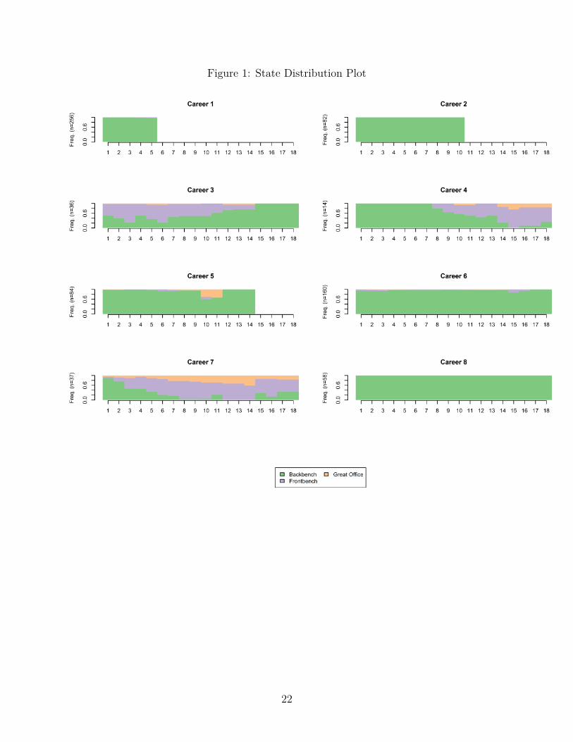
Figure 1: State Distribution Plot

22

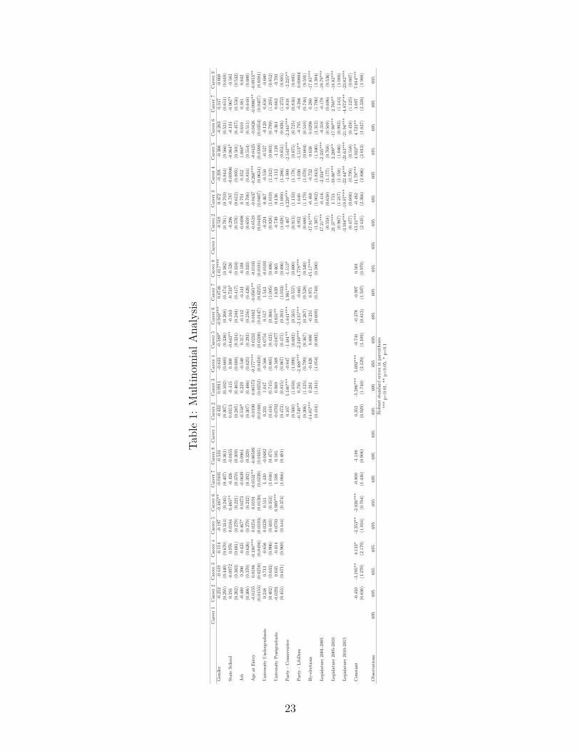
Table1:

Multin

omialA

nalysis

Career1

Career2

Career3

Career4

Career5

Career6

Career7

Career8

Career1

Career2

Career3

Career4

Career5

Career6

Career7

Career8

Career1

Career2

Career3

Career4

Career5

Career6

Career7

Career8

Gen

der

-0.252

-0.419

-0.114

-0.197

-0.485

**-0.010

1-0.534

-0.432

0.09

11-0.633

-0.580

*-0.948

***

0.07

46-1.017

***

-0.518

0.47

2-0.391

-0.366

-0.263

0.31

7-0.668

(0.295

)(0.440)

(0.670)

(0.314

)(0.245

)(0.407

)(0.361

)(0.307

)(0.502

)(0.669

)(0.336

)(0.268

)(0.474

)(0.382)

(0.701

)(0.703

)(0.844

)(0.566

)(0.521

)(0.651

)(0.610

)StateScho

ol0.19

1-0.097

20.97

60.01

840.46

5**

-0.426

-0.045

50.03

13-0.415

0.30

8-0.643

**-0.163

-0.733

*-0.520

-0.296

-0.787

-0.009

46-0.964

*-0.191

-0.967

*-0.583

(0.262

)(0.383)

(0.681)

(0.279

)(0.221

)(0.370

)(0.309

)(0.285

)(0.465

)(0.688

)(0.324

)(0.244

)(0.417

)(0.334)

(0.576

)(0.612

)(0.805

)(0.501

)(0.457

)(0.556

)(0.532

)Jo

b-0.480

0.20

0-0.435

0.46

7*0.03

73-0.063

90.09

04-0.558

*0.22

9-0.540

0.31

7-0.142

-0.141

-0.108

-0.049

80.79

10.35

21.06

8*0.61

00.38

10.84

2(0.306

)(0.370)

(0.626

)(0.279

)(0.232

)(0.392

)(0.329

)(0.307

)(0.486

)(0.625

)(0.293

)(0.256

)(0.426

)(0.333)

(0.659

)(0.706

)(0.834

)(0.554

)(0.511

)(0.648

)(0.600

)Age

atEn

try

-0.015

50.01

86-0.180

***

0.02

540.01

91-0.053

1**

-0.005

89-0.019

00.00

573

-0.177

***

0.02

330.01

62-0.050

1**

-0.010

3-0.051

9-0.043

7-0.260

***

-0.042

5-0.042

6-0.0980*

*-0.095

3**

(0.015

5)(0.025

8)(0.049

4)(0.019

3)(0.013

0)(0.023

9)(0.016

5)(0.016

8)(0.025

2)(0.045

8)(0.020

8)(0.014

7)(0.022

5)(0.018

1)(0.044

9)(0.040

7)(0.063

4)(0.038

8)(0.035

4)(0.040

7)(0.038

1)University

Und

ergrad

uate

0.24

80.71

3-0.656

0.02

280.51

11.43

0-0.048

20.23

11.04

7-0.566

0.07

540.517

1.54

3-0.0593

-0.224

0.46

7-0.550

-0.527

-0.120

0.85

0-0.680

(0.402

)(0.633)

(0.906

)(0.403

)(0.353

)(1.046

)(0.475

)(0.416

)(0.745

)(0.865

)(0.423

)(0.366

)(1.005

)(0.486)

(0.928

)(1.019

)(1.242

)(0.803

)(0.799

)(1.205

)(0.852

)University

Postgrad

uate

-0.029

10.63

5-0.414

0.07

030.98

9***

1.58

80.58

5-0.070

20.96

9-0.569

-0.047

70.83

1**

1.63

90.46

5-0.749

0.13

6-1.112

-1.139

-0.361

0.66

3-0.793

(0.455

)(0.671)

(0.969

)(0.444

)(0.374

)(1.066

)(0.481

)(0.473

)(0.815

)(0.967

)(0.475

)(0.391

)(1.033

)(0.496)

(1.028

)(1.088

)(1.286

)(0.851

)(0.826

)(1.272

)(0.885

)Pa

rty-C

onservative

0.10

75.14

6***

-0.847

-1.481

**-1.641

***

1.98

1***

-1.513*

-1.407

4.22

0***

-1.909

-2.543

***

-2.341

***

0.81

8-2.225

**(0.500

)(1.050

)(1.099

)(0.692

)(0.565

)(0.557

)(0.800)

(0.913

)(1.133

)(1.178

)(0.875

)(0.725)

(0.816

)(0.895

)Pa

rty-L

ibDem

-0.749

**0.79

5-2.488

***

-2.249

***

-2.115

***

-0.665

-1.778

***

-0.952

1.64

0-1.036

-1.513

**-0.795

-0.266

0.00

884

(0.306

)(1.125

)(0.799

)(0.367

)(0.267

)(0.528

)(0.349)

(0.688

)(1.179

)(1.070

)(0.604

)(0.510)

(0.746

)(0.591

)By-electio

ns-14.85

***

0.28

1-0.426

0.80

0-0.231

0.97

1-15.17

***

-17.91

***

-0.468

-0.732

0.63

80.02

980.28

0-17.85

***

(0.416

)(1.341

)(1.054

)(0.693

)(0.609

)(0.740

)(0.500)

(1.387

)(1.902

)(1.843

)(1.340

)(1.312)

(1.706

)(1.304

)Le

gisla

ture

2001

-200

517

.21*

**-0.416

-2.334

**-2.335

***

-0.318

-0.179

-19.79

***

(0.558

)(0.638

)(1.177

)(0.768

)(0.509

)(0.696

)(0.536

)Le

gisla

ture

2005

-201

021

.37*

**1.75

3-18.00

***

2.20

9**

-17.90

***

2.76

0**

-18.82

***

(0.987

)(1.217

)(1.158

)(1.046

)(0.993

)(1.143

)(1.016

)Le

gisla

ture

2010

-201

5-3.594

***

-19.87

***

-22.44

***

-21.63

***

-21.94

***

-4.873

***

-23.02

***

(0.477

)(0.606

)(0.795

)(0.558

)(0.458

)(1.125

)(0.607

)Con

stan

t-0.450

-3.195

**4.13

3*-2.353

**-2.036

***

-0.800

-1.188

0.35

3-5.286

***

5.69

2***

-0.741

-0.278

-0.907

0.50

1-13.21

***

-0.482

11.78*

**4.92

3**

4.72

3**

3.69

77.01

4***

(0.836

)(1.270)

(2.179

)(1.034

)(0.704

)(1.436

)(0.906

)(0.929

)(1.740

)(2.129

)(1.109

)(0.813

)(1.507

)(0.979

)(2.435

)(2.366

)(2.806

)(2.013

)(1.837

)(2.328

)(1.988

)

Observatio

ns69

569

569

569

569

569

569

569

569

569

569

569

569

569

569

569

569

569

569

569

569

569

569

569

5Rob

uststan

dard

errors

inpa

renthe

ses

***p<

0.01

,**p<

0.05

,*p<

0.1

23